Quantum non-Markovian “casual bystander” environments

Abstract

Quantum memory effects can be induced even when the degrees of freedom associated to the environment are not affected at all during the system evolution. In this paper, based on a bipartite representation of the system-environment dynamics, we found the more general interactions that lead to this class of quantum non-Markovian “casual bystander environments.” General properties of the resulting dynamics are studied with focus on the system-environment correlations, a collisional measurement-based representation, and the quantum regression hypothesis. Memory effects are also characterized through an operational approach, which in turn allows to detect when the studied properties apply. Single and multipartite qubits dynamics support and exemplify the developed results.

I Introduction

Both in classical and quantum realms, memory effects emerge whenever a set of dynamical degrees of freedom is not considered as part of the system of interest vanKampen ; breuerbook ; vega ; wiseman . In classical systems (or incoherent ones), the presence of memory effects can be related to departures from a Markov property defined in a probabilistic frame. In contrast, the definition of memory effects and non-Markovianity is much more subtle in a quantum regime.

Given that any quantum system is affected by a measurement process, a reasonable approach to defining quantum non-Markovianity is to study the properties of the (unperturbed) system density matrix propagator. In fact, the theory of quantum semigroups alicki  is usually taken as a landmark of quantum Markovianity. Thus, any departure of the propagator properties with respect to that of a Lindblad evolution can be proposed as a signature of quantum non-Markovianity BreuerReview ; plenioReview . This approach has shown to be a very fruitful tool to study memory effects in quantum systems, leading to the formulation of many, in general inequivalent, memory witnesses (see for example Refs. BreuerFirst ; EnergyBackFLow ; Energy ; HeatBackFLow ; rivas ; DarioSabrina ; canonicalCresser ). One interesting perspective that these studies provide is the understanding of memory effects through an “environment-to-system backflow of information” BreuerFirst ; EnergyBackFLow ; Energy ; HeatBackFLow . Information stored in the environment degrees of freedom may influence the system at later times, giving a solid and clear understanding of memory effects.

In spite of the simplicity and efficacy of the previous theoretical perspective, it has been shown that memory effects may emerge even when the degrees of freedom associated to the environment are not affected at all during the system evolution, which implies the absence of any “physical” environment-to-system backflow of information. A clear situation where this occurs is in quantum systems coupled to incoherent degrees of freedom that have a fixed classical stochastic dynamics megier ; maximal .

While the previous drawback in the definition of information flows remains under debate megier ; maximal ; petruccione ; amato ; santis ; acin ; horo ; EntroBack , alternative operational approaches to quantum memory effects modi ; pollock ; pollockInfluence ; goan ; budiniCPF ; budiniChina ; bonifacio ; han ; BIF ; ban furnish a possible solution. For example, by subjecting a system to three successive measurements, a conditional past-future correlation budiniCPF  provides a memory witness that is consistent with the usual probabilistic approach to non-Markovianity. This object is defined by the correlation between the first and last outcomes conditioned to a given intermediate value. It vanishes in a (probabilistic) Markovian regime. In addition, by randomizing the intermediate post-measurement system state, even in presence of memory effects, the conditional past-future correlation vanishes when the environment is not affected by the system evolution BIF . Thus, it detects the presence or absence of “bidirectional system-environment information flows.” This last property provides a solution to the previous drawback. In fact, a solid experimental procedure for distinguishing between memory effects induced by environments that are affected or not by their interaction with the system is established.

The previous advancements left open an interesting issue whose formulation is independent of any memory witness definition. Besides environments consisting of incoherent degrees of freedom with a fixed classical stochastic dynamics, in which other situations it may occur that the environment is not affected at all by its interaction with the system? More specifically, we ask about the most general system-environment interactions that guarantee this property. The resolution of this problem is relevant for achieving a clear understanding of intrinsically different memory effects, that is, those where the environment is or not altered by its interaction with the system.

The main goal of this work is to answer the previous question. We characterize the most general system-environment interactions that, even when the system develops memory effects, guarantee that the environment self-dynamics and state remain independent of the system degrees of freedom. For these “casual bystander environments,” special interest is paid to the resulting system dynamics, the system-environment correlations, a collisional measurement-based representation embedding ; collisionVacchini ; ciccarello ; palmaMultipartito ; strunz ; portugal ; brasilCollisional ; brasil , and the validity of the quantum regression hypothesis when analyzing system operator correlations QRTVacchini ; QRTLindbladRate ; mutual ; banQRT . General expressions for the conditional past-future correlation budiniCPF ; BIF are also provided. The main results are exemplified by studying these properties and indicators for a class of qubit dynamics with single and multipartite dephasing channels.

The paper is outlined as follows. In Sec. II we derive the most general interaction consistent with a causal bystander environment. General properties of the resulting system dynamics are analyzed in Sec. III. In Sec. IV we study single and multipartite examples. The conclusions are provided in Sec. V. Calculus details are presented in the Appendix.

II Quantum “casual bystander” environments

We consider a system ($s$) interacting with uncontrollable quantum degrees of freedom that constitute the environment ($e$). Correspondingly, in the total Hilbert space $\mathcal{H}_{s}\otimes\mathcal{H}_{e},$ the bipartite density matrix is denoted as $\rho_{t}^{se}.$ Its evolution is written as

$$\frac{d}{dt}\rho_{t}^{se}=(\mathcal{L}_{s}+\mathcal{L}_{e}+\mathcal{L}_{se})[\rho_{t}^{se}],$$ (1)

where $\mathcal{L}_{s}$ and $\mathcal{L}_{e}$ define the system and environment isolated dynamics respectively, while $\mathcal{L}_{se}$ introduce their mutual interaction. As usual, the marginal system and environment states follow by tracing out the complementary degrees of freedom,

$$\rho_{t}^{s}=\mathrm{Tr}_{e}[\rho_{t}^{se}],\ \ \ \ \ \ \ \ \ \ \ \rho_{t}^{e}=\mathrm{Tr}_{s}[\rho_{t}^{se}],$$ (2)

where $\mathrm{Tr}[\cdots]$ is the trace operation. By definition, a casual bystander environment is characterized by a density matrix $\rho_{t}^{e}$ that is completely independent of the system state and dynamics. Consequently, its time-evolution $(d\rho_{t}^{e}/dt)$ must also fulfill the same property. From Eq. (1) we get $(d\rho_{t}^{e}/dt)=\mathcal{L}_{e}[\rho_{t}^{e}]+\mathrm{Tr}_{s}(\mathcal{L}_{se}[\rho_{t}^{se}]),$ leading to the condition

$$\mathrm{Tr}_{s}(\mathcal{L}_{se}[\rho_{t}^{se}])=\mathcal{A}[\rho_{t}^{e}],$$ (3)

where $\mathcal{A}$ is an arbitrary superoperator acting on $\rho_{t}^{e}.$ This criterion allows us to find which kind of system-environment couplings fulfill the proposed definition.

II.1 Unitary coupling

A unitary coupling is set by a bipartite Hamiltonian $H_{se}$ such that

$$\mathcal{L}_{se}[\bullet]=-i[H_{se},\bullet].$$ (4)

In order to check condition (3), we introduce a complete orthogonal basis $\{|s\rangle\}$ of the system Hilbert space such that $\sum_{s}|s\rangle\langle s|=\mathrm{I}_{s},$ where $\mathrm{I}_{s}$ is the system identity matrix. We get,

$$\mathrm{Tr}_{s}(\mathcal{L}_{se}[\rho_{t}^{se}])=-i\sum_{s,s^{\prime}}\left[\langle s|H_{se}|s^{\prime}\rangle,\langle s^{\prime}|\rho_{t}^{se}|s\rangle\right].$$ (5)

Thus, independence of the environment state of the system degrees of freedom requires $\langle s|H_{se}|s^{\prime}\rangle=\delta_{s,s^{\prime}}Q_{e},$ which in turn implies $H_{se}=I_{s}\otimes Q_{e},$ where $Q_{e}=Q_{e}^{{\dagger}}$ is an arbitrary operator acting on $\mathcal{H}_{e}.$ Nevertheless, this solution implies that system and environment do not interact. Consequently, it is impossible to obtain a casual bystander non-Markovian environment if it interacts unitarily with the system of interest.

The previous result is not valid when a Born-Markov approximation applies breuerbook , where the environment state can be approximated by a stationary one, $\rho_{t}^{e}=\rho_{0}^{e}.$ Nevertheless, in this situation memory effects do not develop.

II.2 Dissipative coupling

After discarding the unitary property, now we consider dissipative system-environment couplings. Thus, the environment is defined by a set of quantum degrees of freedom whose interaction with the system can be approximated by an arbitrary (non-diagonal) Lindblad superoperator breuerbook ,

$$\mathcal{L}_{se}[\bullet]=\sum_{i,j}\gamma_{i,j}(T_{i}\bullet T_{j}^{{\dagger}}-\frac{1}{2}\{T_{j}^{{\dagger}}T_{i},\bullet\}_{+}),$$ (6)

where $\{a,b\}_{+}\equiv ab+ba.$ The complex parameters $\{\gamma_{i,j}\}$ define the (diagonal and nondiagonal) rate coefficients of the dissipative channels corresponding to the bipartite operators $\{T_{i}\}.$ Thus, they constitute an Hermitian positive definite matrix alicki . Under the replacements $T_{i}\rightarrow V_{k}\otimes B_{\alpha},\ T_{j}\rightarrow V_{l}\otimes B_{\beta}$ and $\gamma_{i,j}\rightarrow\gamma_{k\alpha,l\beta},$ where $\{V_{k}\}$ and $\{B_{\alpha}\}$ are arbitrary operators acting on $\mathcal{H}_{s}$ and $\mathcal{H}_{e}$ respectively, $\mathcal{L}_{se}$ can be rewritten as

$$\mathcal{L}_{se}[\bullet]\!=\!\!\sum_{k\alpha,l\beta}\gamma_{k\alpha,l\beta}(V_{k}B_{\alpha}\bullet B_{\beta}^{{\dagger}}V_{l}^{{\dagger}}-\frac{1}{2}\{V_{l}^{{\dagger}}V_{k}B_{\beta}^{{\dagger}}B_{\alpha},\bullet\}_{+}).$$ (7)

Here, the indexes run in the intervals $k,l=1,\cdots,(\dim\mathcal{H}_{s})^{2}-1,$ and $\alpha,\beta=1,\cdots,(\dim\mathcal{H}_{e})^{2}-1.$

By taking the trace to the interaction superoperator $\mathcal{L}_{se}[\rho_{t}^{se}],$ we get

$$\mathrm{Tr}_{s}(\mathcal{L}_{se}[\rho_{t}^{se}])\! = \!\!\sum_{\alpha,\beta,s}\Big{(}B_{\alpha}\langle s|D_{\alpha,\beta}\rho_{t}^{se}|s\rangle B_{\beta}^{{\dagger}}-\frac{1}{2}B_{\beta}^{{\dagger}}B_{\alpha}$$

$$\!\!\!\!\times\langle s|D_{\alpha,\beta}\rho_{t}^{se}|s\rangle-\frac{1}{2}\langle s|\rho_{t}^{se}D_{\alpha,\beta}|s\rangle B_{\beta}^{{\dagger}}B_{\alpha}\Big{)},$$

where as before $\{|s\rangle\}$ is a complete base in $\mathcal{H}_{s}.$ Furthermore, we introduced the system operators $\{D_{\alpha,\beta}\},$

$$D_{\alpha,\beta}\equiv\sum_{k,l}\gamma_{k\alpha,l\beta}V_{l}^{{\dagger}}V_{k},\ \ \ \ \ \ \ \ D_{\alpha,\beta}^{{\dagger}}=D_{\beta,\alpha}.$$ (8)

The Hermitian property is inherited from condition $\rho_{t}^{se}=(\rho_{t}^{se})^{\dagger}$ in Eq. (1). It is simple to realize that the constraint (3) is fulfilled if

$$\langle s|D_{\alpha,\beta}=\Gamma_{\alpha,\beta}\langle s|,\ \ \ \ \ \ \ \ D_{\alpha,\beta}|s\rangle=\Gamma_{\alpha,\beta}|s\rangle,$$ (9)

where $\Gamma_{\alpha,\beta}$ are, in general, complex coefficients. Applying $\sum_{s^{\prime}}|s^{\prime}\rangle$ and $\sum_{s^{\prime}}\langle s^{\prime}|$ to the left and right equalities, using that $D_{\alpha,\beta}^{{\dagger}}=D_{\beta,\alpha},$ we get the equivalent conditions

$$D_{\alpha,\beta}=\Gamma_{\alpha,\beta}\mathrm{I}_{s},\ \ \ \ \ \ \ \ \Gamma_{\alpha,\beta}^{\ast}=\Gamma_{\beta,\alpha}.$$ (10)

Introducing the final constraints (10) into Eq. (7), we can write the bipartite interaction generator as

$$\mathcal{L}_{se}[\bullet]=\sum_{\alpha,\beta}\Gamma_{\alpha,\beta}\ (B_{\alpha}\mathbb{S}_{\alpha,\beta}[\bullet]B_{\beta}^{{\dagger}}-\frac{1}{2}\{B_{\beta}^{{\dagger}}B_{\alpha},\bullet\}_{+}),$$ (11)

where the coefficients $\{\Gamma_{\alpha,\beta}\}$ define an Hermitian positive definite matrix. Furthermore, $\{\mathbb{S}_{\alpha,\beta}\}$ is a set of arbitrary completely positive system superoperators that fulfill the symmetry $\mathbb{S}_{\alpha,\beta}^{{\dagger}}=\mathbb{S}_{\beta,\alpha}$ and are trace preserving, $\mathrm{Tr}_{s}[\mathbb{S}_{\alpha,\beta}[\rho^{s}]]=\mathrm{Tr}_{s}[\rho^{s}].$ Hence, they can be written in a Kraus representation breuerbook as

$$\mathbb{S}_{\alpha,\beta}[\bullet]=\sum_{k}V_{k}^{\alpha\beta}\bullet V_{k}^{{\dagger}\alpha\beta},\ \ \ \ \ \ \ \ \ \ \ \ \ \sum_{k}V_{k}^{{\dagger}\alpha\beta}V_{k}^{\alpha\beta}=\mathrm{I}_{s},$$ (12)

where $V_{k}^{\alpha\beta}$ are (arbitrary) system operators. The bipartite system-environment evolution [Eq. (1)] can finally be written as

$$\frac{d}{dt}\rho_{t}^{se} = (\mathcal{L}_{s}+\mathcal{L}_{e})[\rho_{t}^{se}]+\sum_{\alpha,\beta}\Gamma_{\alpha,\beta}\ B_{\alpha}\mathbb{S}_{\alpha,\beta}[\rho_{t}^{se}]B_{\beta}^{{\dagger}}$$ (13)

$$-\frac{1}{2}\sum_{\alpha,\beta}\Gamma_{\alpha,\beta}\{B_{\beta}^{{\dagger}}B_{\alpha},\rho_{t}^{se}\}_{+},$$

where $\mathcal{L}_{s}$ and $\mathcal{L}_{e}$ are arbitrary. This equation is the main result of this section. It defines the most general dissipative system-environment coupling that is consistent with a quantum non-Markovian casual bystander environment. In fact, after applying the (system) trace operation to Eq. (13), and using the property (12), the density matrix $\rho_{t}^{e}$ of the environment [Eq. (2)] evolves as

$$\frac{d}{dt}\rho_{t}^{e}=\mathcal{L}_{e}[\rho_{t}^{e}]+\sum_{\alpha,\beta}\Gamma_{\alpha,\beta}\ (B_{\alpha}\rho_{t}^{e}B_{\beta}^{{\dagger}}-\frac{1}{2}\{B_{\beta}^{{\dagger}}B_{\alpha},\rho_{t}^{e}\}_{+}).$$ (14)

As expected, this Lindblad equation does not depend on the system degrees of freedom. On the other hand, the time evolution of the system state, $\rho_{t}^{s}=\mathrm{Tr}_{e}[\rho_{t}^{se}],$ assuming uncorrelated initial conditions $\rho_{0}^{se}=\rho_{0}^{s}\otimes\rho_{0}^{e},$ from Eq. (13) can formally be written as a time-convoluted equation,

$$\frac{d}{dt}\rho_{t}^{s}=\mathcal{L}_{s}[\rho_{t}^{s}]+\int_{0}^{t}dt^{\prime}\mathcal{K}_{s}(t-t^{\prime})[\rho_{t^{\prime}}^{s}],$$ (15)

where the superoperator $\mathcal{K}_{s}(t)$ is defined in a Laplace domain $[f(z)=\int_{0}^{\infty}dte^{-zt}f(t)]$ from the relation $\mathrm{Tr}_{e}[\mathcal{G}_{z}^{se}(\mathcal{L}_{e}+\mathcal{L}_{se})\rho_{0}^{e}][\bullet]=\mathrm{Tr}_{e}[\mathcal{G}_{z}^{se}\rho_{0}^{e}]\mathcal{K}_{s}(z)[\bullet],$ where $\mathcal{G}_{z}^{se}=[z-(\mathcal{L}_{s}+\mathcal{L}_{e}+\mathcal{L}_{se})]^{-1}$ is the bipartite system-environment propagator.

Both, Eqs. (13) and (14) can always be reduced to a standard diagonal form breuerbook ; alicki , which can be read by taking $\Gamma_{\alpha,\beta}=\delta_{\alpha,\beta}\Gamma_{\alpha},$ where $\{\Gamma_{\alpha}\}$ are positive rate coefficients. Furthermore, Eq. (15) can always be transformed into a convolutionless form LocalNonLocal .

III General properties

On the basis of Eq. (13), it is possible to establish general properties that characterize the system-environment dynamics.

III.1 System-environment correlations

Even for uncorrelated initial conditions, the evolution (13) induces correlations between the system and the degrees of freedom associated to the environment. These correlations can be characterized from the bipartite state $\rho_{t}^{se}.$ Here, we show that, for uncorrelated initial conditions, $\rho_{0}^{se}=\rho_{0}^{s}\otimes\rho_{0}^{e},$ it always assumes the structure

$$\rho_{t}^{se}=\sum_{c}\rho_{c}(t)\otimes|c_{t}\rangle\langle c_{t}|,$$ (16)

where $\{\rho_{c}(t)\}$ are states (matrixes) in $\mathcal{H}_{s}$ and $\{|c_{t}\rangle\langle c_{t}|\}$ are orthogonal time-dependent projectors in $\mathcal{H}_{e},$ that is, $\langle c_{t}|c_{t}^{\prime}\rangle=\delta_{cc^{\prime}}.\$Consistently, the system and environment states read

$$\rho_{t}^{s}=\sum_{c}\rho_{c}(t),\ \ \ \ \ \ \ \ \ \rho_{t}^{e}=\sum_{c}p_{c}(t)|c_{t}\rangle\langle c_{t}|,$$ (17)

where $p_{c}(t)\equiv\mathrm{Tr}_{s}[\rho_{c}(t)].$ From these expressions, it follows that $\{|c_{t}\rangle\}$ is the base in which $\rho_{t}^{e}$ becomes diagonal at time $t.$ Furthermore, $\rho_{c}(t)$ is the conditional state of the system given that the environment is in the state $|c_{t}\rangle\langle c_{t}|.$

The formal solution (16) implies that $\rho_{t}^{se}$ is a separable state entanglement with a null system-environment discord discord . Hence, not any quantum entanglement (between the system and the environment) is produced during the evolution.

The validity of Eq. (16) can be established from the bipartite evolution (13). From these equations, for the system conditional states $\{\rho_{c}(t)\},$ we get the evolution

$$\frac{D}{Dt}\rho_{c}(t) = \mathcal{L}_{s}[\rho_{c}(t)]+\sum_{\tilde{c}}\phi_{c\tilde{c}}(t)\rho_{\tilde{c}}(t)-\sum_{\tilde{c}}\phi_{\tilde{c}c}(t)\rho_{c}(t)$$ (18)

$$\!\!\!\!\!\!+\sum_{\tilde{c}}\gamma_{c\tilde{c}}(t)\mathbb{S}_{c\tilde{c}}(t)[\rho_{\tilde{c}}(t)]-\sum_{\tilde{c}}\gamma_{\tilde{c}c}(t)\rho_{c}(t).$$

Here, a “total-time-derivative” was introduced,

$$\frac{D}{Dt}\rho_{c}(t)\equiv\frac{d}{dt}\rho_{c}(t)+\sum_{\tilde{c}}\langle c_{t}|\frac{d}{dt}[\Pi_{t}^{\tilde{c}}]|c_{t}\rangle\rho_{\tilde{c}}(t),$$ (19)

where $\Pi_{t}^{c}\equiv|c_{t}\rangle\langle c_{t}|.$ Furthermore, the time-dependent rates are

$$\phi_{c\tilde{c}}(t)=\langle c_{t}|\mathcal{L}_{e}[\Pi_{t}^{\tilde{c}}]|c_{t}\rangle\geq 0,$$ (20)

and similarly

$$\gamma_{\tilde{c}c}(t)=\sum_{\alpha,\beta}\Gamma_{\alpha,\beta}\ \langle c_{t}|B_{\alpha}|\tilde{c}_{t}\rangle\langle\tilde{c}_{t}|B_{\beta}^{{\dagger}}|c_{t}\rangle\geq 0,$$ (21)

where the inequality follows straightforwardly from the diagonal rate representation $\Gamma_{\alpha,\beta}=\delta_{\alpha,\beta}\Gamma_{\alpha}.$ Finally, in Eq. (18) the system superoperators $\mathbb{S}_{c\tilde{c}}(t)[\bullet]$ read

$$\mathbb{S}_{c\tilde{c}}(t)[\bullet]=\frac{\sum_{\alpha,\beta}\Gamma_{\alpha,\beta}\ \langle c_{t}|B_{\alpha}|\tilde{c}_{t}\rangle\langle\tilde{c}_{t}|B_{\beta}^{{\dagger}}|c_{t}\rangle\mathbb{S}_{\alpha,\beta}[\bullet]}{\sum_{\alpha,\beta}\Gamma_{\alpha,\beta}\ \langle c_{t}|B_{\alpha}|\tilde{c}_{t}\rangle\langle\tilde{c}_{t}|B_{\beta}^{{\dagger}}|c_{t}\rangle},$$ (22)

which are trace preserving, $\mathrm{Tr}_{s}[\mathbb{S}_{c\tilde{c}}(t)[\rho]]=\mathrm{Tr}_{s}[\rho].$ The system superoperators $\mathbb{S}_{\alpha,\beta}[\bullet]$ are defined by Eq. (12).

On the other hand, the evolution of the probabilities $\{p_{c}(t)\}$ [Eq. (17)] follows by taking the trace of Eq. (18), which yields

$$\frac{D}{Dt}p_{c}(t) = +\sum_{\tilde{c}}\phi_{c\tilde{c}}(t)p_{\tilde{c}}(t)-\sum_{\tilde{c}}\phi_{\tilde{c}c}(t)p_{c}(t)$$ (23)

$$\!\!+\sum_{\tilde{c}}\gamma_{c\tilde{c}}(t)p_{\tilde{c}}(t)-\sum_{\tilde{c}}\gamma_{\tilde{c}c}(t)p_{c}(t).$$

Here, $(D/Dt)p_{c}(t)$ follows from Eq. (19) under the replacement $\rho_{c}(t)\rightarrow p_{c}(t).$ Consistently, this equation does not depend on the system degrees of freedom.

The consistence of the time evolution of $\rho_{c}(t)$ and $p_{c}(t)$ [Eqs. (18) and (23) respectively] supports the structure defined by Eq. (16). The physical meaning of these results can be easily understood by analyzing an incoherent environment case.

III.2 Incoherent environment

If the degrees of freedom of the environment do not develop any (quantum) coherence, at any time its density matrix $\rho_{t}^{e}$ is diagonal in a fixed base $\{|c\rangle\}.$ Thus, the previous results must be read under the replacement

$$|c_{t}\rangle\langle c_{t}|\rightarrow|c\rangle\langle c|.$$ (24)

In consequence, the total-time-derivative [Eq. (19)] becomes an usual time-derivative, $(D/Dt)\rightarrow(d/dt),$ and the rates $\phi_{c\tilde{c}}(t)$ and $\gamma_{\tilde{c}c}(t)$ do not depend on time. In this situation, the probabilities $\{p_{c}(t)\}$ obey a standard classical master equation [Eq. (23)]. Similarly, the evolution of the states $\{\rho_{c}(t)\}$ [Eq. (18)] involves the same classical coupling with rates $\phi_{c\tilde{c}},$ while the coupling with rates $\gamma_{c\tilde{c}}$ are endowed by the application of the superoperators $\mathbb{S}_{c\tilde{c}}$ in each environment transition $c\leftarrow\tilde{c}.$ Thus, the evolution becomes a particular case corresponding to a system driven by incoherent degrees of freedom that follows their own stochastic dynamics (see Eq. (27) in Ref. maximal ).

When condition (24) is not fulfilled, the interpretation of Eqs. (18) and (23) remains the same as in the incoherent case. Nevertheless, the base $\{|c_{t}\rangle\}$ associated to the environment become time-dependent due to the intrinsic quantum nature of the environment degrees of freedom. This effect is taken into account through the total-time-derivative $D/Dt$ [Eq. (19)].

III.3 Measurement based stochastic representation

A clear understanding of the system-environment coupling can be achieved by representing their dynamics with a measurement-based carmichaelbook ; plenio stochastic bipartite state $\rho_{st}^{se}(t).$ Thus, in average over realizations (denoted with an overbar symbol) it follows

$$\rho_{t}^{se}=\overline{\rho_{st}^{se}(t)}.$$ (25)

In principle, the state $\rho_{st}^{se}(t)$ can be formulated from the incoherent-like representation (18). A deeper understanding is achieved by assuming that the degrees of freedom of the environment are subjected to continuous-in-time measurement process that resolves the transitions induced by the (bath) operators $\{B_{\alpha}\}.$ Thus, $\rho_{st}^{se}(t)$ follows from the standard quantum jump approach carmichaelbook ; plenio (for simplicity we consider in Eqs. (13) and (14) the diagonal case $\Gamma_{\alpha,\beta}=\delta_{\alpha,\beta}\Gamma_{\alpha},$ denoting $\mathbb{S}_{\alpha,\alpha}\leftrightarrow\mathbb{S}_{\alpha}).$ The environment state is recovered as $\rho_{t}^{e}=\overline{\rho_{st}^{e}(t)},$ where $\rho_{st}^{e}(t)=\mathrm{Tr}_{s}[\rho_{st}^{e}(t)].$ For a casual bystander environment, the evolution of $\rho_{st}^{e}(t)$ is independent of the system dynamics, being defined by the transitions associated to $\{B_{\alpha}\}.$ Similarly, from the evolution (13) it follows that the bipartite state (assuming uncorrelated initial conditions), must to take the form

$$\rho_{st}^{sa}(t)=\rho_{st}^{s}(t)\otimes\rho_{st}^{e}(t).$$ (26)

It is simple to realize that the dynamics of the system state $\rho_{st}^{s}(t)$ must include the action of the superoperator $\mathbb{S}_{\alpha}$ whenever the environment suffers a transition (jump) corresponding to the operator $B_{\alpha}.$ In this way, the bipartite system-environment correlations [Eq. (16)] are built up in average. On the other hand, between environment transitions, the state $\rho_{st}^{s}(t)$ evolves under the action of $\mathcal{L}_{s}.$ Thus, the system dynamics can be seen as a collisional one collisionVacchini ; embedding , where the occurrence of the sudden (collisional) changes $\rho_{st}^{s}\rightarrow\mathbb{S}_{\alpha}[\rho_{st}^{s}]$ are dictated by the environment transitions associated to the operator $B_{\alpha}.$ We notice that this representation recover the results of Ref. embedding , which can be read as a particular case of the general dynamics (13).

III.4 Quantum regression hypothesis

The underlying system-environment dynamics is Markovian [Eq. (13)]. Thus, the quantum regression theorem (QRT) carmichaelbook is valid in the bipartite space $\mathcal{H}_{s}\otimes\mathcal{H}_{e}.$ Introducing a vector of system operators $\mathbf{A\leftrightarrow A}\otimes\mathrm{I}_{e},$ where $\mathbf{A}=(A_{1},A_{2,}\cdots,A_{\dim(\mathcal{H}_{s})^{2}}),$ their expectation value at a time $\tau$ (for simplicity, also denoted with an overbar symbol) can be written as

$$\overline{\mathbf{A}(\tau)}=\mathrm{Tr}_{se}(\mathcal{G}_{\tau,0}^{se}[\rho_{0}^{se}]\mathbf{A}).$$ (27)

The bipartite propagator is $\mathcal{G}_{\tau,\tau_{0}}^{se}\equiv\exp[(\tau-\tau_{0})\mathcal{L}_{T}],$ with $\mathcal{L}_{T}\equiv(\mathcal{L}_{s}+\mathcal{L}_{e}+\mathcal{L}_{se}),$ where $\mathcal{L}_{se}$ follows from Eq. (13). Given an extra system operator $O\leftrightarrow O\otimes\mathrm{I}_{e},$ the correlations $\overline{O(t)\mathbf{A}(t+\tau)}$ follow from the QRT, which implies carmichaelbook

$$\overline{O(t)\mathbf{A}(t+\tau)}=\mathrm{Tr}_{se}(\mathbf{A}\mathcal{G}_{t+\tau,t}^{se}[\rho_{t}^{se}O\mathbb{]}).$$ (28)

Now, we search conditions under which the QRT is valid on $\mathcal{H}_{s}.$ Thus, we explore if the previous (system) operator correlations can be written only in terms of the system propagator. Assuming uncorrelated initial conditions, $\rho_{0}^{se}=\rho_{0}^{s}\otimes\rho_{0}^{e},$ the system propagator $\mathcal{G}_{\tau,0}^{s}$ can be written as

$$\mathcal{G}_{\tau,0}^{s}[\bullet]\equiv\mathrm{Tr}_{e}(\mathcal{G}_{\tau,0}^{se}[\bullet]\otimes\rho_{0}^{e}]).$$ (29)

Thus, from Eq. (27), the operator expectation values can be rewritten as

$$\overline{\mathbf{A}(\tau)}=\mathrm{Tr}_{s}(\mathcal{G}_{\tau,0}^{s}[\rho_{0}^{s}]\mathbf{A}).$$ (30)

On the other hand, it is simple to realize that the correlations (28) cannot be written only in terms of the system propagator $\mathcal{G}_{t+\tau,t}^{s},$ which implies that the QRT is not valid in general on $\mathcal{H}_{s}.$ Nevertheless, assuming that the environment begins in its stationary state $(\rho_{\mathrm{\infty}}^{e}),$ and that the stationary bipartite state $(\lim\nolimits_{t\rightarrow\infty}\rho_{t}^{se})$ do not involve system-environment correlations,

$$\rho_{0}^{se}=\rho_{0}^{s}\otimes\rho_{\mathrm{\infty}}^{e},\ \ \ \ \ \ \ \ \ \ \ \ \lim\nolimits_{t\rightarrow\infty}\rho_{t}^{se}=\rho_{\mathrm{\infty}}^{s}\otimes\rho_{\mathrm{\infty}}^{e},$$ (31)

in the long time limit the operator correlations become

$$\lim\nolimits_{t\rightarrow\infty}\overline{O(t)\mathbf{A}(t+\tau)}=\mathrm{Tr}_{s}(\mathbf{A}\mathcal{G}_{\tau,0}^{s}[\rho_{\mathrm{\infty}}^{s}O\mathbb{]}).$$ (32)

Thus, if the conditions (31) are fulfilled the QRT is valid in the stationary regime even when the system dynamics is non-Markovian. Interestingly, the same property arises in quantum systems coupled to arbitrary incoherent degrees of freedom QRTLindbladRate . In fact, given that none condition on $\mathcal{G}_{\tau,0}^{se}$ was demanded in the previous derivation, this result is valid in general whenever the bipartite (system-environment) dynamics is a Markovian (Lindblad) one. The explicit meaning of the restricted validity of the QRT becomes clear by writing $\overline{\mathbf{A}(\tau)}=\boldsymbol{\hat{T}}(\tau)\overline{\mathbf{A}(0)},$ and the stationary correlations as $\lim\nolimits_{t\rightarrow\infty}\overline{O(t)\mathbf{A}(t+\tau)}=\boldsymbol{\hat{T}}(\tau)\lim\nolimits_{t\rightarrow\infty}\overline{O(t)\mathbf{A}(t)},$ where $\boldsymbol{\hat{T}}(\tau)$ is a matrix in the space corresponding to the vector of operators $\overline{\mathbf{A}(0)}$ carmichaelbook .

III.5 Operational memory witness

Memory effects can alternatively be characterized from measurement-based approaches. A conditional past-future (CPF) correlation budiniCPF is defined by a set of three successive measurements performed over the system of interest. Here, they are taken as projective ones, corresponding to Hermitian operators $O_{\underline{\mathbf{m}}},$ denoted in successive order with$\ \underline{\mathbf{m}}=\underline{\mathbf{x}},\underline{\mathbf{y}},\underline{\mathbf{z}}.$ Their eigenvectors and eigenvalues read $O_{\underline{\mathbf{m}}}|m\rangle=m|m\rangle,\$where correspondingly $\{m\}=\{x\},$ $\{y\},$ $\{z\}.$ The measurements are performed at the initial time $t=0$ (past), at time $t$ (present) and $t+\tau$ (future) respectively. After the intermediate measurement at time $t,$ the system post-measurement state is externally modified BIF as $\rho_{y}=|y\rangle\langle y|\rightarrow\rho_{\breve{y}}=|\breve{y}\rangle\langle\breve{y}|.$ A deterministic scheme (d) is defined by the condition $\breve{y}=y.$ Thus, not any change is introduced. A random scheme (r) is defined by a random election of $\breve{y}$ (over the set $\{y\}$) with and arbitrary probability $\wp(\breve{y}|x),$ which may depend on the outcomes $\{x\}$ of the first measurement performed at time $t=0.$ The CPF correlation depends on the chosen scheme. In both cases, it reads

$$C_{pf}(t,\tau)|_{\breve{y}}\overset{d/r}{=}\sum_{z,x}zx[P(z,x|\breve{y})-P(z|\breve{y})P(x|\breve{y})],$$ (33)

where $\{z\}$ and $\{x\}$ are the eigenvalues of $O_{\underline{\mathbf{z}}}$ and $O_{\underline{\mathbf{x}}}$ respectively. With $P(a|b)$ we denote the conditional probability of $a$ given $b.$

In the deterministic scheme, the CPF correlation vanishes in a Markovian regime, where past and future outcomes are conditionally independent: $P(z,x|\breve{y})=P(z|\breve{y})P(x|\breve{y})$ budiniCPF . Thus, $C_{pf}(t,\tau)|_{\breve{y}}\overset{d}{\neq}0$ detects memory effects independently of their underling mechanism. This last property can be understood from the change of the bipartite state $\rho_{se}$ after the intermediate (projective) measurement,

$$\rho_{se}\rightarrow|y\rangle\langle y|\otimes\frac{\langle y|\rho_{se}|y\rangle}{\mathrm{Tr}_{se}[|y\rangle\langle y|\rho_{se}]}.$$ (34)

The dependence of the environment post-measurement state $\langle y|\rho_{se}|y\rangle/\mathrm{Tr}_{se}[|y\rangle\langle y|\rho_{se}]$ on the previous system history (measurement outcomes at the initial time) allows to detect memory effects.

In the random scheme, even in presence of memory effects, the CPF correlation vanishes when the environment is not affected during the system evolution BIF . Consequently, the presence of a (non-Markovian) casual bystander environment implies that $C_{pf}(t,\tau)|_{\breve{y}}\overset{r}{=}0.$ Alternatively, in the random scheme, the condition $C_{pf}(t,\tau)|_{\breve{y}}\overset{r}{\neq}0$ indicates departures with respect to a casual bystander environment, here defined by the condition Eq. (3).

The previous features of the random scheme can be understood from Eq. (34) by introducing the random system transformation $|y\rangle\langle y|\rightarrow|\breve{y}\rangle\langle\breve{y}|$ and averaging (marginating) the environment post-measurement states (associated to the outcomes $\{y\}$) with their probabilities $\{\mathrm{Tr}_{se}[|y\rangle\langle y|\rho_{se}]\}.$ Thus, after the intermediate measurement the bipartite state transform as

$$\rho_{se}\rightarrow|\breve{y}\rangle\langle\breve{y}|\otimes\sum_{y}\langle y|\rho_{se}|y\rangle=|\breve{y}\rangle\langle\breve{y}|\otimes\mathrm{Tr}_{s}[\rho_{se}].$$ (35)

From the definition of a casual bystander environment [see also Eq. (3)], it follows that the (bath) state $\mathrm{Tr}_{s}[\rho_{se}]$ does not depend on the previous (system) history, which implies that a Markov property characterize the outcome statistics. Consequently, the CPF correlation vanishes.

The conditional probabilities appearing in Eq. (33) can explicitly be calculated from the joint outcome probability $P(z,\check{y},x)\leftrightarrow P(z,t+\tau;\check{y},t;x,0).$ As shown in Refs. budiniCPF ; BIF , this object can be calculated after knowing the system-environment propagator. In order to maintain a description as simple as possible, we consider Eq. (13) in the diagonal case $\Gamma_{\alpha,\beta}=\delta_{\alpha,\beta}\Gamma_{\alpha}$ (denoting $\mathbb{S}_{\alpha,\alpha}\leftrightarrow\mathbb{S}_{\alpha}$) and assuming that the composition of two arbitrary superoperators can be written as a superoperator included in the master equation, that is, $\mathbb{S}_{\alpha}\mathbb{S}_{\alpha^{\prime}}=\mathbb{S}_{\alpha^{\prime\prime}}.$ Under these two conditions, the bipartite propagator, $\rho_{t}^{se}=\mathcal{G}_{t,0}^{se}[\rho_{0}^{s}\otimes\rho_{0}^{e}],$ can be written in a general way as

$$\rho_{t}^{se}=\rho_{0}^{s}\otimes\mathcal{F}_{0}(t)[\rho_{0}^{e}]+\sum_{\begin{subarray}{c}\alpha\\ \alpha\neq 0\end{subarray}}\mathbb{S}_{\alpha}[\rho_{0}^{s}]\otimes\mathcal{F}_{\alpha}(t)[\rho_{0}^{e}].$$ (36)

Here, the environment superoperators $\{\mathcal{F}_{\alpha}(t)\},$ which act on the initial environment state $\rho_{0}^{e},$ depend on each specific problem.

III.5.1 Deterministic scheme

In the deterministic scheme, the joint outcome probability can be written as BIF

$$\frac{P(z,\breve{y},x)}{P(x)}\overset{d}{=}\mathrm{Tr}_{se}(E_{z}\mathcal{G}_{t+\tau,t}^{se}[\rho_{\breve{y}}\otimes\mathrm{Tr}_{s}(E_{\breve{y}}\mathcal{G}_{t,0}^{se}[\rho_{x}^{se}])]).$$ (37)

Here, $E_{m}\equiv|m\rangle\langle m|,$ $\rho_{m}\equiv|m\rangle\langle m|$ $[m=z,\breve{y},x]$ and $\rho_{x}^{se}\equiv\rho_{x}\otimes\rho_{0}^{e}.$ Furthermore, $P(x)=\langle x|\rho_{0}^{s}|x\rangle.$ From this expression, using the bipartite propagator (36), we get

$$\frac{P(z,\check{y},x)}{P(x)}\overset{d}{=}\sum_{\alpha,\beta}\langle z|\mathbb{S}_{\alpha}[\rho_{\check{y}}]|z\rangle\langle\check{y}|\mathbb{S}_{\beta}[\rho_{x}]|\check{y}\rangle$$

$$\ \ \ \ \ \ \ \ \ \ \ \ \ \ \ \ \ \times\mathrm{Tr}_{e}[\mathcal{F}_{\alpha}(\tau)\mathcal{F}_{\beta}(t)\rho_{0}^{e}\mathbb{].}$$ (38)

Using that $P(z,x|\breve{y})=P(z,\breve{y},x)/P(\breve{y}),$ where $P(\breve{y})=\sum_{z,x}P(z,\breve{y},x),$ the CPF correlation (33) reads

$$C_{pf}(t,\tau)|_{\breve{y}}\overset{d}{=}\frac{1}{P(\breve{y})^{2}}\sum_{\alpha,\beta,\mu}\Theta^{\alpha\beta\mu}|_{\breve{y}}\Lambda_{\alpha\beta\mu}(t,\tau).$$ (39)

The time-independent coefficients $\Theta^{\alpha\beta\mu}|_{y}$ only depend on the chosen observables,

$$\Theta^{\alpha\beta\mu}|_{\breve{y}}=\langle\breve{y}|\mathbb{S}_{\alpha}^{\#}[O_{\underline{\mathbf{z}}}]|\breve{y}\rangle\langle\breve{y}|\mathbb{S}_{\beta}[O_{\underline{\mathbf{x}}}\rho_{\underline{\mathbf{x}}}]|\breve{y}\rangle\langle\breve{y}|\mathbb{S}_{\mu}[\rho_{\underline{\mathbf{x}}}]|\breve{y}\rangle,$$ (40)

where the dual superoperator $\mathbb{S}_{\alpha}^{\#}$ is defined from $\mathrm{Tr}_{s}(O\mathbb{S}_{\alpha}[\rho])=\mathrm{Tr}_{s}(\rho\mathbb{S}_{\alpha}^{\#}[O]).$ Furthermore, we defined the state $\rho_{\underline{\mathbf{x}}}\equiv\sum_{x}P(x)|x\rangle\langle x|=\sum_{x}\langle x|\rho_{0}^{s}|x\rangle|x\rangle\langle x|.$ The time-dependence in Eq. (39) follows from

$$\Lambda_{\alpha\beta\mu}(t,\tau) = +\mathrm{Tr}_{e}[\mathcal{F}_{\alpha}(\tau)\mathcal{F}_{\beta}(t)\rho_{0}^{e}]\ \mathrm{Tr}_{e}[\mathcal{F}_{\mu}(t)\rho_{0}^{e}]$$

$$-\mathrm{Tr}_{e}[\mathcal{F}_{\alpha}(\tau)\mathcal{F}_{\mu}(t)\rho_{0}^{e}]\ \mathrm{Tr}_{e}[\mathcal{F}_{\beta}(t)\rho_{0}^{e}],$$

which only depends on the initial environment state $\rho_{0}^{e}$ and environment superoperators $\{\mathcal{F}_{\alpha}(t)\}.$ The probability $P(\breve{y})$ is

$$P(\breve{y})=\sum_{\alpha}\langle\breve{y}|\mathbb{S}_{\alpha}[\rho_{\underline{\mathbf{x}}}]|\breve{y}\rangle\mathrm{Tr}_{e}[\mathcal{F}_{\alpha}(t)\rho_{0}^{e}].$$ (42)

The previous formula give an exact analytical expression for the CPF correlation that is valid for a broad class of problems (see Sec. IV below).

III.5.2 Random scheme

In the random scheme, $P(z,\breve{y},x)$ reads BIF

$$\frac{P(z,\breve{y},x)}{P(x)}\overset{r}{=}\mathrm{Tr}_{se}(E_{z}\mathcal{G}_{t+\tau,t}^{se}[\rho_{\breve{y}}\otimes\mathrm{Tr}_{s}(\mathcal{G}_{t,0}^{se}[\rho_{x}^{se}])])\wp(\breve{y}|x),$$ (43)

where as before $E_{m}\equiv|m\rangle\langle m|,$ $\rho_{m}\equiv|m\rangle\langle m|$ $[m=z,\breve{y},x],$ and $\rho_{x}^{se}\equiv\rho_{x}\otimes\rho_{0}^{e},$ while $P(x)=\langle x|\rho_{0}^{s}|x\rangle.$ Furthermore, the conditional probability $\wp(\breve{y}|x)$ can be freely chosen. Using the propagator expression (36), it follows

$$\frac{P(z,\check{y},x)}{P(x)}\overset{r}{=}\sum_{\alpha}\langle z|\mathbb{S}_{\alpha}[\rho_{\check{y}}]|z\rangle\mathrm{Tr}_{e}[\mathcal{F}_{\alpha}(\tau)\rho_{t}^{e}]\wp(\check{y}|x).$$ (44)

Consequently, independently of the chosen measurement observables, it is confirmed that the CPF correlation [Eq. (33)] vanishes identically in this scheme,

$$C_{pf}(t,\tau)|_{\breve{y}}\overset{r}{=}0.$$ (45)

In fact, the sum term $[\sum_{\alpha}\cdots]$ in Eq. (44) can be read as $P(z|\check{y}),$ leading to the Markovian structure $P(z,\check{y},x)=$ $P(z|\check{y})\wp(\check{y}|x)P(x)\rightarrow P(z,x|\check{y})=P(z|\check{y})P(x|\check{y}).$

IV Examples

In order to exemplify the developed results, we consider different single and multipartite system dynamics interacting with a quantum casual bystander environment.

IV.1 Single qubit system

The system is a qubit, while the quantum degrees of freedom of the environment correspond to a two-level fluorescent system with decay rate $\gamma$ and Rabi frequency $\Omega$ carmichaelbook . Their mutual evolution [Eq. (13)] is written as

$$\frac{d}{dt}\rho_{t}^{se}=-i\frac{\Omega}{2}[\sigma_{x},\rho_{t}^{se}]+\gamma\Big{(}\sigma\mathbb{S}[\rho_{t}^{se}]\sigma^{{\dagger}}-\frac{1}{2}\{\sigma^{{\dagger}}\sigma,\rho_{t}^{se}\}_{+}\Big{)}.$$ (46)

The operators $\sigma_{x},$ $\sigma^{{\dagger}},$ and $\sigma$ are respectively the $x$-Pauli matrix and the raising and lowering operators in the two-dimensional environment Hilbert space $\mathcal{H}_{e}.$ The unique system contribution is the superoperator [see Eq. (12)]

$$\mathbb{S}[\bullet]=\sigma_{z}\mathbb{[}\bullet]\sigma_{z},$$ (47)

where $\sigma_{z}$ is the $z$-Pauli matrix in the system Hilbert space $\mathcal{H}_{s}.$ Thus, the system is subjected to a dephasing process driven by the transitions of the fluorescent system.

IV.1.1 System-environment propagator

Considering (bipartite) uncorrelated initial conditions, $\rho_{0}^{se}=\rho_{0}^{s}\otimes\rho_{0}^{e},$ the propagator of Eq. (46) can be written with the structure (36),

$$\rho_{t}^{se}=\rho_{0}^{s}\otimes\mathcal{F}_{+}(t)[\rho_{0}^{e}]+\mathbb{S}[\rho_{0}^{s}]\otimes\mathcal{F}_{-}(t)[\rho_{0}^{e}].$$ (48)

At any time, this bipartite state is a separable one [Eq. (16)]. Consistently, a positive partial transpose criterion entanglement is fulfilled. On the other hand, the environment superoperators $\mathcal{F}_{\pm}$ can be written as

$$\mathcal{F}_{\pm}(t)[\bullet]=\frac{1}{2}(\mathcal{G}_{t,0}^{+}[\bullet]\pm\mathcal{G}_{t,0}^{-}[\bullet]),$$ (49)

where the auxiliary superoperators $\mathcal{G}_{t}^{\pm}[\bullet]$ are defined by the evolutions,

$$\frac{d}{dt}\mathcal{G}_{t,t_{0}}^{\pm}\!\!=\!\!-i\frac{\Omega}{2}[\sigma_{x},\mathcal{G}_{t,t_{0}}^{\pm}]+\gamma\Big{(}\pm\sigma\mathcal{G}_{t,t_{0}}^{\pm}\sigma^{{\dagger}}-\frac{1}{2}\{\sigma^{{\dagger}}\sigma,\mathcal{G}_{t,t_{0}}^{\pm}\}_{+}\Big{)},$$ (50)

with the initial conditions $\mathcal{G}_{t_{0,}t_{0}}^{\pm}=\mathrm{I}_{e}.$ These equations can be solved in an analytical way.

Both superoperators $\mathcal{G}_{t,t_{0}}^{\pm}$ define the system and environment dynamics,

$$\rho_{t}^{e}=\mathcal{G}_{t,0}^{+}[\rho_{0}^{e}],\ \ \ \ \ \ \ \ f(\tau|t)\equiv\mathrm{Tr}_{e}(\mathcal{G}_{t+\tau,t}^{-}[\rho_{t}^{e}]).$$ (51)

In fact, from Eqs. (46) and (50) it is simple to realize that $\mathcal{G}_{t,t_{0}}^{+}$ is the propagator of the environment degrees of freedom. Furthermore, from Eq. (48) it is simple to show that the function$\ f(\tau|t)$ sets the system coherence decay,

$$\rho_{t}^{s}=\left(\begin{array}[]{cc}p_{up}&f(t|0)c_{up}\\ f(t|0)c_{dn}&p_{dn}\end{array}\right),$$ (52)

where $p_{up}$ and $p_{dn}$ are the initial upper and lower system populations while the nondiagonal contributions $c_{up}$ and $c_{dn}$ are the initial system coherences. Furthermore,

$$f(\tau|t)=e^{-\gamma\tau}a_{t}+e^{-\gamma\tau/4}\Big{[}b_{t}\cosh(\Delta\tau)+c_{t}\frac{\sinh(\Delta\tau)}{\Delta}\Big{]},$$ (53)

where for shortening the expression we introduced the coefficient $\Delta\equiv\sqrt{(\gamma/4)^{2}-\Omega^{2}}.$ Explicit expressions for the time-dependent coefficients $a_{t},$ $b_{t},$ and $c_{t},$ can be found in the Appendix.

IV.1.2 Operator correlations

From Eq. (48), using that $\lim_{t\rightarrow\infty}\mathcal{G}_{t,t_{0}}^{+}[\rho_{0}^{e}]=\rho_{\infty}^{e}$ and $\lim_{t\rightarrow\infty}\mathcal{G}_{t,t_{0}}^{-}[\rho_{0}^{e}]=0,$ it follows

$$\lim\nolimits_{t\rightarrow\infty}\rho_{t}^{se}=\rho_{\mathrm{\infty}}^{s}\otimes\rho_{\mathrm{\infty}}^{e},\ \ \ \ \ \ \rho_{\mathrm{\infty}}^{s}=\frac{1}{2}(\rho_{0}^{s}+\mathbb{S}[\rho_{0}^{s}]),$$ (54)

where $\rho_{\mathrm{\infty}}^{e}$ is the stationary state of a two-level fluorescent system (see Appendix). Thus, when the environment at the initial time begins in its stationary state, the conditions (31) are fulfilled, indicating the validity of the QRT in the stationary regime. This conclusion is corroborated by the following explicit calculation of operator expectation values and correlations. Nevertheless, we also found that for some operator correlations, the QRT is valid at all times.

Introducing the vector of system operators $\mathbf{\sigma}\equiv\{\sigma_{x},\sigma_{y},\sigma_{z}\},$ their expectation values, from Eq. (27), read

$$\overline{\mathbf{\sigma}(\tau)}=\boldsymbol{\hat{T}}(\tau|0)\ \overline{\mathbf{\sigma}(0)},$$ (55)

where $\overline{\mathbf{\sigma}(0)}=\mathrm{Tr}_{s}[\mathbf{\sigma}(0)\rho_{0}^{s}].$ Similarly, for the Pauli operators there are nine possible correlations $\overline{\sigma_{i}(t)\sigma_{j}(t+\tau)}.$ For six of them, from Eq. (28) we get

$$\overline{\sigma_{x}(t)\mathbf{\sigma}(t+\tau)} = \boldsymbol{\hat{T}}(\tau|t)\ \overline{\sigma_{x}(t)\mathbf{\sigma}(t)},$$ (56a)

$$\overline{\sigma_{y}(t)\mathbf{\sigma}(t+\tau)} = \boldsymbol{\hat{T}}(\tau|t)\ \overline{\sigma_{y}(t)\mathbf{\sigma}(t)}.$$ (56b)

In these expressions, the matrix $$\boldsymbol{\hat{T}}(\tau|t)$$ reads

$$\boldsymbol{\hat{T}}(\tau|t)=\mathrm{diag}\{f(\tau|t),f(\tau|t),1\}.$$ (57)

When the environment begins in its stationary state $\rho_{0}^{e}=\rho_{\infty}^{e}=\lim_{t\rightarrow}\rho_{t}^{e},$ it follows that $f(\tau|t)=f(\tau|0)$ [see Eq. (51)], and consequently $\boldsymbol{\hat{T}}(\tau|t)=\boldsymbol{\hat{T}}(\tau|0).$ Thus, the six correlations (56) at any time $(t$ and $\tau)$ evolve as the expectation values [Eq. (55)] indicating the absence of any departure with respect to the QRT.

The unique correlations [Eq. (28)] that depart  (at any finite time) from the predictions of the QRT are

$$\overline{\sigma_{z}(t)\mathbf{\sigma}(t+\tau)}=\boldsymbol{\tilde{T}}(\tau,t)\overline{\sigma_{z}(t)\mathbf{\sigma}(t)},$$ (58)

where the matrix $\boldsymbol{\tilde{T}}(\tau,t)$ is

$$\boldsymbol{\tilde{T}}(\tau,t)=\mathrm{diag}\left\{\frac{f(t+\tau|0)}{f(t|0)},\frac{f(t+\tau|0)}{f(t|0)},1\right\}.$$ (59)

If the semigroup property $f(t+\tau|0)=f(\tau|t)f(t|0)$ becomes valid, the QRT is recovered. This happens when the system coherence can be approximated by an exponential decay behavior. On the other hand, using that $\overline{\sigma_{z}(t)\mathbf{\sigma}(t)}=\mathrm{diag}\{f(t|0),f(t|0),1\}\overline{\sigma_{z}(0)\mathbf{\sigma}(0)}$ we get $\lim_{t\rightarrow\infty}\overline{\sigma_{z}(t)\mathbf{\sigma}(t)}=\{0,0,1\}.$ Thus, consistently with Eq. (31), in the long time limit the correlations (58) obey the same evolution as the operator expectation values [Eq. (55)], $\lim_{t\rightarrow\infty}\overline{\sigma_{z}(t)\mathbf{\sigma}(t+\tau)}=\boldsymbol{\hat{T}}(\tau|0)\{0,0,1\},$ indicating the validity of the QRT in the stationary regime.

IV.1.3 Memory witnesses

A deeper understanding of the memory effects developed in the studied model can be achieved by comparing operational and non-operational memory witnesses.

For non-operational approaches, the central ingredient to analyze is the system density matrix evolution. From Eq. (52), straightforwardly we get

$$\frac{d}{dt}\rho_{t}^{s}=\frac{1}{2}\gamma_{t}(\mathbb{S}[\rho_{t}^{s}]-\rho_{t}^{s}),\ \ \ \ \ \gamma_{t}=-\frac{d}{dt}\ln[f(t|0)],$$ (60)

where $f(t|0)$ follows from Eq. (53).

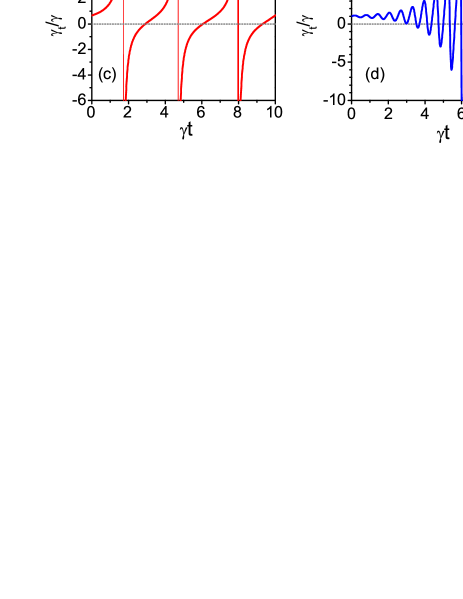
Figure 1: Time dependence of the decoherence rate Eq. (60) corresponding to the underlying dynamics (46). The environment begins in its stationary state. In each plot, the parameters are (a) $\Omega/\gamma=1/10,$ (b) $\Omega/\gamma=1/4,$ (c) $\Omega/\gamma=1,$ and (d) $\Omega/\gamma=10.$

The negativity of $\gamma_{t}$ can be used as an indicator of memory effects canonicalCresser . We assume that the environment begins in its stationary state, $\rho_{0}^{e}=\rho_{\infty}^{e}.$ Thus, $f(\tau|t)=f(\tau|0)$ [see Eq. (51)]. In Fig. 1 we plot $\gamma_{t}$ for different values of the quotient $\Omega/\gamma.$ For $\Omega/\gamma\leq 1/4$ the rate is always positive, while for $\Omega/\gamma>1/4$ it develops periodical divergences. Thus, the dynamics is non-Markovian in this last regime. The same conclusion follows from the trace distance between two initial states BreuerFirst . On the other hand, for $\Omega/\gamma\gg 1/4,$ the rate $\gamma_{t}$ approach a constant value, implying that a Markovian regime is reached again.

The previous rate behaviors can be understood from the underlying environment dynamics. For $\Omega/\gamma\ll 1/4,$ the probability distribution of the elapsed time between environment (fluorescent) transitions approach an exponential function with average time $[2\Omega^{2}/\gamma]^{-1}$ carmichaelbook . Consequently, the coherence decay function (induced by the application of the superoperator $\mathbb{S}$) can be approximated as $f(\tau|0)\approx\exp[-t(2\Omega^{2}/\gamma)],$ which implies $\gamma_{t}\approx 2\Omega^{2}/\gamma$ [Fig. 1(a)]. This regime changes drastically when $\Omega/\gamma=1/4$ [Fig. 1(b)], where the environment starts to develop Rabi oscillations. Around $\Omega/\gamma\approx 1,$ the system coherence $f(t|0)$ vanishes in a oscillatory way. Consequently, $\gamma_{t}$ [Eq. (60)] develops periodic divergences [Fig. 1(c)]. For $\Omega/\gamma\gg 1,$ the effect of the (fast) environment Rabi oscillations over the system cancel out in average, leading to the coherence decay $f(\tau|0)\approx\exp(-t\gamma).$ Thus, $\gamma_{t}\approx\gamma.$ This tendency is clearly seen in Fig. 1(d) at the initial stage.

The previous dynamical regimes can be analyzed from the operational approach. For the dynamics (46), using the explicit propagator Eq. (48), all statistical objects that define the CPF correlation can explicitly be evaluated. We consider that the three consecutive measurements are performed in the $\hat{x}$-direction of the system Bloch sphere. Thus, in all cases, the possible measurement outcomes (eigenvalues) are $m=\pm 1$ $(m=x,y,z),$ while the corresponding eigenvectors are $|m\rangle=|up\rangle+m|dn\rangle,$ where $|up\rangle$ and $|dn\rangle$ are respectively the upper and down states of the system [see Eq. (52)].

In the deterministic scheme, the joint outcome probability Eq. (38) becomes

$$P(z,\breve{y},x)\overset{d}{=}\frac{1}{4}[1+z\breve{y}f(\tau|t)+zxf(t+\tau|0)+\breve{y}xf(t|0)]P(x).$$ (61)

The CPF correlation Eq. (39) reads

$$C_{pf}(t,\tau)|_{\breve{y}}\overset{d}{=}\frac{1-\langle x\rangle^{2}}{4[P(\breve{y})]^{2}}[f(t+\tau|0)-f(\tau|t)\ f(t|0)],$$ (62)

with $P(\breve{y})=[1+\breve{y}\langle x\rangle f(t|0)]/2,$ jointly with $\langle x\rangle=\sum_{x=\pm 1}xP(x)$ and $P(x)=\langle x|\rho_{0}^{s}|x\rangle$ where $\{|x\rangle\}$ are the eigenvectors of the $\hat{x}$-Pauli matrix.

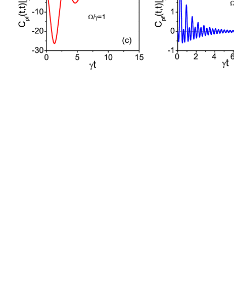
Figure 2: CPF correlation [Eq. (62)] with equal time intervals $\tau=t$ corresponding to the system-environment model (46). The parameters $\Omega/\gamma$ are the same than in Fig. 1. Similarly, the environment begins in its stationary state. In all cases, the system initial condition is such that $\langle x\rangle=0.$

In Fig. 2, for the same parameter regimes shown in Fig. 1, we plot the CPF correlation at equal time intervals, $\tau=t.$ The environment also begins in its stationary state, $\rho_{0}^{e}=\rho_{\infty}^{e}.$

Contrarily to the non-operational memory witnesses, the CPF correlation indicates the presence of memory effects for all parameter regimes, even when the rate $\gamma_{t}$ is positive at all times. Consistently, for $\Omega/\gamma\ll 1/4,$ the maximal absolute value of the CPF correlation diminishes [Fig. 2(a)], indicating the proximity of a Markovian regime. When $\Omega/\gamma=1/4$ [Fig. 2(b)], the CPF is negative at all times and does not develop oscillations. For $\Omega/\gamma\approx 1,$ it develops oscillations and its absolute value is maximal [Fig. 2(c)], indicating strong memory effects. Consistently, when $\Omega/\gamma\gg 1,$ the CPF correlation oscillates but with a smaller amplitude [Fig. 2(d)], indicating again the approaching of a Markov regime.

Contrarily to memory witnesses based only on the unperturbed system dynamics, the CPF correlation indicates a Markovian regime only in the limits $\Omega/\gamma\rightarrow 0$ and $\Omega/\gamma\rightarrow\infty.$ In addition, the operational approach gives a much deeper characterization when considering the random scheme. From Eq. (44), for the joint probabilities we get

$$P(z,\breve{y},x)\overset{r}{=}\frac{1}{2}[1+z\breve{y}f(\tau|t)]\wp(\breve{y}|x)P(x).$$ (63)

As expected, a Markovian property is fulfilled, leading consistently to $C_{pf}(t,\tau)|_{\breve{y}}\overset{r}{=}0$ [Eq. (45)] for arbitrary initial environment states. This result indicates the presence of a casual bystander environment, property that cannot be resolved with non-operational approaches.

IV.2 Multipartite qubit systems

The developed formalism also allows to study the coupling of multipartite systems with a casual bystander environment. In contrast to Eq. (46), here we consider a set of $N$ qubits. For simplicity, we assume the system-environment evolution

$$\frac{d}{dt}\rho_{t}^{se}\! = \!-i\frac{\Omega}{2}[\sigma_{x},\rho_{t}^{se}]+\gamma\Big{(}\sigma\mathbb{S}_{\underline{\mathbf{a}}}[\rho_{t}^{se}]\sigma^{{\dagger}}-\frac{1}{2}\{\sigma^{{\dagger}}\sigma,\rho_{t}^{se}\}_{+}\Big{)}$$ (64)

$$+\varphi\Big{(}\sigma^{{\dagger}}\mathbb{S}_{\underline{\mathbf{b}}}[\rho_{t}^{se}]\sigma-\frac{1}{2}\{\sigma\sigma^{{\dagger}},\rho_{t}^{se}\}_{+}\Big{)},$$

As before, $\sigma_{x},$ $\sigma^{{\dagger}},$ and $\sigma$ are respectively the $x$-Pauli matrix and the raising and lowering operators in the two-dimensional environment Hilbert space $\mathcal{H}_{e}.$ Thus, the environment corresponds to a two-level fluorescent-like system with Rabi frequency $\Omega,$ decay rate $\gamma,$ while the rate $\varphi$ scales the presence of thermally induced excitations breuerbook .

Each of the system superoperators $\mathbb{S}_{\mathbf{\alpha}}[\bullet]\equiv\sigma_{\mathbf{\alpha}}\bullet\sigma_{\mathbf{\alpha}}$ $(\mathbf{\alpha}=\underline{\mathbf{a}},\underline{\mathbf{b}})$ are defined by an arbitrary (multipartite) Pauli string $\sigma_{\mathbf{\alpha}}=\sigma_{\alpha_{1}}\otimes\cdots\otimes\sigma_{\alpha_{N}},$ which consists in the external product of $N$ arbitrary Pauli operators acting on each qubit. These superoperators are applied over the system whenever the environment suffers a transition between its (two) states. From Eq. (64), it follows that $\mathbb{S}_{\underline{\mathbf{a}}}$ is applied when an environmental transition between the upper and lower states occurs, while $\mathbb{S}_{\underline{\mathbf{b}}}$ is applied for the inverse (thermally-induced) transition.

The bipartite propagator associated to Eq. (64) can be written with the structure Eq. (36). The label of the superoperators $\{\mathcal{F}_{\mathbf{\alpha}}(t)\}$ runs over the values $\mathbf{\alpha}=\mathbf{0},\underline{\mathbf{a}},\underline{\mathbf{b}},\underline{\mathbf{c}},$ where $\mathbb{S}_{\underline{\mathbf{c}}}=\mathbb{S}_{\underline{\mathbf{b}}}\mathbb{S}_{\underline{\mathbf{a}}}.$ The calculations that lead to explicit solutions for the environment superoperators $\{\mathcal{F}_{\mathbf{\alpha}}(t)\}$ are presented in the Appendix. From these expressions and Eq. (36), it follows that

$$\lim\nolimits_{t\rightarrow\infty}\rho_{t}^{se}=\rho_{\mathrm{\infty}}^{s}\otimes\rho_{\mathrm{\infty}}^{e},\ \ \ \ \ \rho_{\mathrm{\infty}}^{s}=\frac{1}{4}(\rho_{0}^{s}+\sum_{\alpha}\mathbb{S}_{\alpha}[\rho_{0}^{s}]),$$ (65)

where $\rho_{\mathrm{\infty}}^{s}$ is the multipartite system stationary state while the (two-level) state $\rho_{\mathrm{\infty}}^{e}$ follows by tracing out the system degrees of freedom in Eq. (64). In consequence, as in the previous example, the QRT is valid for stationary correlations of the system.

From Eq. (36) the system state at any time, $\rho_{t}^{s}=\mathrm{Tr}_{e}(\rho_{t}^{se}),$ can straightforwardly be written as a statistical superposition of Kraus maps,

$$\rho_{t}^{s}=p_{t}^{\mathbf{0}}\rho_{0}+\sum_{\mathbf{\alpha}=\underline{\mathbf{a}},\underline{\mathbf{b}},\underline{\mathbf{c}},}p_{t}^{\mathbf{\alpha}}\mathbb{S}_{\mathbf{\alpha}}[\rho_{0}],$$ (66)

where the weights are $p_{t}^{\mathbf{\alpha}}\equiv\mathrm{Tr}_{e}[\mathcal{F}_{\alpha}(t)[\rho_{0}^{e}]].$ Similarly, the density matrix evolution can be written as

$$\frac{d\rho_{t}^{s}}{dt}=\sum_{\mathbf{\alpha}=\underline{\mathbf{a}},\underline{\mathbf{b}},\underline{\mathbf{c}},}\gamma_{t}^{\mathbf{\alpha}}(\mathbb{S}_{\mathbf{\alpha}}[\rho_{t}^{s}]-\rho_{t}^{s}).$$ (67)

Simple expressions for the probabilities $\{p_{t}^{\mathbf{\alpha}}\}$ and rates $\{\gamma_{t}^{\mathbf{\alpha}}\}$ are obtained when $\varphi=\gamma$ in Eq. (64). We get

$$p_{t}^{\mathbf{0}} = \frac{1}{2}e^{-\gamma t}\Big{[}\cosh(\gamma t)+\frac{\gamma^{2}}{\chi^{2}}\cos(\chi t)+\frac{\Omega^{2}}{\chi^{2}}\Big{]},$$ (68a)

$$p_{t}^{\underline{\mathbf{a}}} = p_{t}^{\underline{\mathbf{b}}}=\frac{1}{4}[1-e^{-2\gamma t}],$$ (68b)

$$p_{t}^{\underline{\mathbf{c}}} = \frac{1}{2}e^{-\gamma t}\Big{[}\cosh(\gamma t)-\frac{\gamma^{2}}{\chi^{2}}\cos(\chi t)-\frac{\Omega^{2}}{\chi^{2}}\Big{]},$$ (68c)

where $$\chi\equiv\sqrt{\gamma^{2}+\Omega^{2}}.$$ From these expressions, the rates in Eq. (67) are

$$\gamma_{t}^{\underline{\mathbf{a}}}=\gamma_{t}^{\underline{\mathbf{b}}}=\frac{1}{2}\gamma,\ \ \ \ \ \ \ \gamma_{t}^{\underline{\mathbf{c}}}=\frac{1}{2}\frac{\chi\sin(\chi t)}{(\Omega/\gamma)^{2}+\cos(\chi t)}.$$ (69)

Notice that $\gamma_{t}^{\underline{\mathbf{c}}}$ presents an oscillatory behavior at any time, which develops divergences only when $(\Omega/\gamma)^{2}<1.$ When $\Omega=0,$ it reduces to $\gamma_{t}^{\underline{\mathbf{c}}}=(1/2)\gamma\tan(\gamma t),$ recovering the rates of the “trigonometric eternal non-Markovian” dynamics introduced in Ref. arxiv , where the environment dynamics is an incoherent one. Thus, we can read Eq. (64) as a quantum (coherent) generalization $(\Omega\neq 0)$ of the incoherent environment studied in arxiv .

The CPF correlation can also be obtained in the present case. Assuming that the three measurements correspond to the observable $\sigma_{\mathbf{\alpha}}$ $(\alpha=\underline{\mathbf{a}}$ or $\underline{\mathbf{b}}),$ from Eq. (39) we get (with $\varphi=\gamma)$

$$\!\!\!\!\!\!\!\!C_{pf}(t,\tau)|_{\breve{y}}\overset{d}{=}-\frac{(1-\langle x\rangle^{2})}{[2^{N}P(\breve{y})]^{2}}e^{-(t+\tau)\gamma/2}\Big{[}\frac{\gamma^{2}}{\chi^{2}}\sin(t\chi)\sin(\tau\chi)$$

$$\ \ \ \ \ \ \ \ \ \ \ \ \ \ -\frac{4\gamma^{2}\Omega^{2}}{\chi^{4}}\sin^{2}(t\chi/2)\sin^{2}(\tau\chi/2)\Big{]},$$ (70)

where as before $\chi=\sqrt{\gamma^{2}+\Omega^{2}},$ and $P(\breve{y})=2^{-N}\{1+\breve{y}\langle x\rangle e^{-\gamma t}[\Omega^{2}+\gamma^{2}\cos(t\chi)]/\chi^{2}\}.$ Furthermore, $\langle x\rangle=\sum_{x}x\langle x|\rho_{0}^{s}|x\rangle,$ where $\{x\}$ and $\{|x\rangle\}$ are respectively the eigenvalues and eigenvectors associated to the first measurement observable. When the three measurements correspond to the observable $\sigma_{\underline{\mathbf{c}}},$ we get the accidental vanishing $C_{pf}(t,\tau)|_{y}\overset{d}{=}0.$ On the other hand, in the random scheme Eq. (45) guarantee that $C_{pf}(t,\tau)|_{y}\overset{r}{=}0$ for any system observables and initial environment states.

V Summary and conclusions

Quantum memory effects can be induced by environments whose state and dynamical behavior are not affected at all by their interaction with the system of interest. Based on a bipartite representation of the system-environment dynamics, in this paper we have explored the most general interaction structures that are consistent with this class of non-Markovian casual bystander environments.

While unitary interactions must be discarded, we have found the most general dissipative coupling structures [Eq. (13)] that are consistent with the demanded constraint. The degrees of freedom associated to the environment are governed by a Lindblad evolution. The corresponding system dynamic turns out to be defined by a set of arbitrary completely positive transformations whose action is conditioned to the environment dynamics.

The bipartite system-environment state can always be written as a separable one [Eq. (16)], indicating the absence of quantum entanglement between both parts. Nevertheless, in contrast to a purely incoherent case, the environment may develop quantum coherent behaviors. Consistently, by subjecting the degrees of freedom of the environment to a continuous-in-time measurement process, a product state characterizes the bipartite stochastic dynamics [Eq. (26)], where a collisional dynamics defines the stochastic system evolution.

Similarly to incoherent environments, here the QRT is not valid in general. Nevertheless, stationary (system) operators correlations evolves in the same way as expectation values when the bipartite system-environment stationary state is an uncorrelated one [Eq. (31)]. Consequently, outside the stationary regime operator correlations can be used as a witness of memory effects. Nevertheless, given that the absence of stationary system-environment correlations may emerges in different models, a deeper characterization of non-Markovianity can be achieved through an operational approach.

The CPF correlation is an operational memory witness that relies on performing three consecutive measurement processes over the system of interest. This object was explicitly calculated in terms of a bipartite propagator [Eq. (36)] associated to the studied system-environment coupling. In a deterministic scheme, where the system state is not modified after the intermediate measurement, the CPF correlation detects departure with respect to a (probabilistic) Markovian regime [Eq. (39)]. In a random scheme, where the intermediate post-measurement state is selected in a random way, the CPF correlation vanishes when the environment is a casual bystander one [Eq. (45)]. This feature provides an explicit experimental procedure for detecting when the studied properties apply.

All previous conclusions were supported by the explicit study of single and multipartite qubits dynamics. The developed approach furnishes a solid basis for constructing alternative underlying mechanisms that lead to quantum memory effects. On the other hand, added to incoherent environments with a classical self fluctuating dynamics, the studied dynamics define the most general situation where quantum memory effects are not endowed with a physical environment-to-system backflow of information. While unitary system-environment interactions were discarded, the present results motivate us to ask about different dynamical regimes where an effective non-Markovian casual bystander environmental action could be recovered.

Appendix A Auxiliary expressions and calculus details

Auxiliary expressions and calculation details are provided.

A.1 Coefficients of the coherence decay function

The coherence decay function $f(\tau|t)\equiv\mathrm{Tr}_{e}(\mathcal{G}_{t+\tau,t}^{-}[\rho_{t}^{e}]),$ where $\mathcal{G}_{t+\tau,t}^{-}$ is defined by the evolution (50), can be written as in Eq. (53), where the time-dependent coefficients are

$$a_{t} = \left[1-\frac{2\gamma\Omega\overline{\sigma_{y}(t)}-\overline{\sigma_{z}(t)}\gamma^{2}}{\gamma^{2}+2\Omega^{2}}\right],$$ (71a)

$$b_{t} = \frac{2\gamma\Omega\overline{\sigma_{y}(t)}-\overline{\sigma_{z}(t)}\gamma^{2}}{\gamma^{2}+2\Omega^{2}},$$ (71b)

$$c_{t} = -\frac{6\gamma\Omega\overline{\sigma_{y}(t)}+\overline{\sigma_{z}(t)}(\gamma^{2}+8\Omega^{2})}{4(\gamma^{2}+2\Omega^{2})}.$$ (71c)

The overbar symbol denotes the expectation values $$\overline{\sigma_{i}(t)}=\mathrm{Tr}_{e}[\rho_{t}^{e}\sigma_{i}], \sigma_{i} \mathcal{H}_{e}. \rho_{t}^{e}=\mathcal{G}_{t,0}^{+}[\rho_{0}^{e}], \mathcal{G}_{t,0}^{+} \rho_{\mathrm{\infty}}^{e}=\lim_{t\rightarrow\infty}\rho_{t}^{e}$$ where are Pauli operators in The environment state follows from where is also defined by the evolution (50). The stationary environment state reads

$$\rho_{\mathrm{\infty}}^{e}=\frac{1}{\gamma^{2}+2\Omega^{2}}\left(\begin{array}[]{cc}\Omega^{2}&-i\gamma\Omega\\ +i\gamma\Omega&\gamma^{2}+\Omega^{2}\end{array}\right).$$ (72)

Assuming that the environment begins in this state, the previous expectations values $\overline{\sigma_{i}(\infty)}=\lim_{t\rightarrow\infty}\overline{\sigma_{i}(t)}=\mathrm{Tr}_{e}[\rho_{\infty}^{e}\sigma_{i}]$ follows straightforwardly,

$$\overline{\sigma_{y}(\infty)}=\frac{2\gamma\Omega}{\gamma^{2}+2\Omega^{2}},\ \ \ \ \ \ \ \overline{\sigma_{z}(\infty)}=-\frac{\gamma^{2}}{\gamma^{2}+2\Omega^{2}}.$$ (73)

A.2 Multipartite system-environment propagator

The bipartite propagator corresponding to the model (64) can be written as in Eq. (36). The solution for the set of environment superoperators $\{\mathcal{F}_{\mathbf{\alpha}}(t)\}$ can be obtained by defining the vector

$$\mathcal{F}\equiv\{\mathcal{F}_{\mathbf{0}}(t),\mathcal{F}_{\underline{\mathbf{a}}}(t),\mathcal{F}_{\underline{\mathbf{b}}}(t),\mathcal{F}_{\underline{\mathbf{c}}}(t)\}.$$ (74)

It is written as $\mathcal{F}=(1/4)H\cdot\mathcal{G},$ where $H$ is a four-dimensional Hadamard matrix, $H=\{\{1,1,1,1\},\{1,1,-1,-1\},\{1,-1,1,-1\},\{1,-1-,1,1\}\}.$ The components of the vector $\mathcal{G}$ are denoted as

$$\mathcal{G}\equiv\{\mathcal{G}_{t,0}^{++},\mathcal{G}_{t,0}^{+-},\mathcal{G}_{t,0}^{-+},\mathcal{G}_{t,0}^{--}\},$$ (75)

which in turn can be written as $\mathcal{G}=H\cdot\mathcal{F}.$ With these definitions, the underlying model (64) implies the time-evolutions

$$\frac{d\mathcal{G}^{uv}}{dt}\!\! = \!\!-i\frac{\Omega}{2}[\sigma_{x},\mathcal{G}^{uv}]\!-\!\frac{\gamma}{2}\{\sigma^{{\dagger}}\sigma,\mathcal{G}^{uv}\}_{+}\!-\!\frac{\varphi}{2}\{\sigma\sigma^{{\dagger}},\mathcal{G}^{uv}\}_{+}$$ (76)

$$\!+u(\gamma\sigma\mathcal{G}^{uv}\sigma^{{\dagger}})+v(\varphi\sigma^{{\dagger}}\mathcal{G}^{uv}\sigma),$$

with initial conditions $\mathcal{G}_{t_{0},t_{0}}^{uv}=\mathrm{I}_{e}.$ For shortening the expressions, we denoted $\mathcal{G}_{t,t_{0}}^{uv}\leftrightarrow\mathcal{G}^{uv}.$ The supra indexes are $u=\pm$ and $v=\pm.$ The explicit analytical expressions for the four superoperators $\mathcal{G}^{uv}$ can be obtained by solving their evolution via Laplace transform techniques.

References

- (1) N. G. van Kampen, Stochastic Processes in Physics and Chemistry, (North-Holland, Amsterdam, 1992).
- (2) H. P. Breuer and F. Petruccione, The theory of open quantum systems, (Oxford University press, 2002).
- (3) I. de Vega and D. Alonso, Dynamics of non-Markovian open quantum systems, Rev. Mod. Phys. 89, 015001 (2017).
- (4) L. Li, M. J. W. Hall, and H. M. Wiseman, Concepts of quantum non-Markovianity: A hierarchy, Phys. Rep. 759, 1 (2018).
- (5) R. Alicki and K. Lendi, Quantum Dynamical Semigroups and Applications, Lect. Notes Phys. 717 (Springer, Berlin Heidelberg, 2007).
- (6) H. P. Breuer, E. M. Laine, J. Piilo, and V. Vacchini, Colloquium: Non-Markovian dynamics in open quantum systems, Rev. Mod. Phys. 88, 021002 (2016); H. P. Breuer, Foundations and measures of quantum non-Markovianity, J. Phys. B 45, 154001 (2012).
- (7) A. Rivas, S. F. Huelga, and M. B. Plenio, Quantum non-Markovianity: characterization, quantification and detection, Rep. Prog. Phys. 77, 094001 (2014).
- (8) H. P. Breuer, E. M. Laine, and J. Piilo, Measure for the Degree of Non-Markovian Behavior of Quantum Processes in Open Systems, Phys. Rev. Lett. 103, 210401 (2009); E. M. Laine, J. Piilo, and H. P. Breuer, Measure for the non-Markovianity of quantum processes, Phys. Rev. A 81, 062115 (2010).
- (9) G. Guarnieri, C. Uchiyama, and B. Vacchini, Energy backflow and non-Markovian dynamics, Phys. Rev. A 93, 012118 (2016).
- (10) G. Guarnieri, J. Nokkala, R. Schmidt, S. Maniscalco, and B. Vacchini, Energy backflow in strongly coupled non-Markovian continuous-variable systems, Phys. Rev. A 94, 062101 (2016).
- (11) R. Schmidt, S. Maniscalco, and T. Ala-Nissila, Heat flux and information backflow in cold environments, Phys. Rev. A 94, 010101(R) (2016).
- (12) A. Rivas, S. F. Huelga, and M. B. Plenio, Entanglement and Non-Markovianity of Quantum Evolutions, Phys. Rev. Lett. 105, 050403 (2010).
- (13) D. Chruściński and S. Maniscalco, Degree of Non-Markovianity of Quantum Evolution, Phys. Rev. Lett. 112, 120404 (2014).
- (14) M. J. W. Hall, J. D. Cresser, L. Li, and E. Andersson, Canonical form of master equations and characterization of non-Markovianity, Phys. Rev. A 89, 042120 (2014).
- (15) N. Megier, D. Chruściński, J. Piilo, and W. T. Strunz, Eternal non-Markovianity: from random unitary to Markov chain realisations, Sci. Rep. 7, 6379 (2017).
- (16) A. A. Budini, Maximally non-Markovian quantum dynamics without environment-to-system backflow of information, Phys. Rev. A 97, 052133 (2018).
- (17) F. A. Wudarski and F. Petruccione, Exchange of information between system and environment: Facts and myths, Euro Phys. Lett. 113, 50001 (2016).
- (18) H. P. Breuer, G. Amato, and B. Vacchini, Mixing-induced quantum non-Markovianity and information flow, New J. Phys. 20, 043007 (2018).
- (19) D. De Santis and M. Johansson, Equivalence between non-Markovian dynamics and correlation backflows, New J. Phys. 22, 093034 (2020).
- (20) D. De Santis, M. Johansson, B. Bylicka, N. K. Bernardes, and A. Acín, Witnessing non-Markovian dynamics through correlations, Phys. Rev. A 102, 012214 (2020).
- (21) M. Banacki, M. Marciniak, K. Horodecki, and P. Horodecki, Information backflow may not indicate quantum memory, arXiv:2008.12638.
- (22) N. Megier, A. Smirne, and B. Vacchini, Entropic Bounds on Information Backflow, Phys. Rev. Lett. 127, 030401 (2021).
- (23) F. A. Pollock, C. Rodríguez-Rosario, T. Frauenheim, M. Paternostro, and K. Modi, Operational Markov Condition for Quantum Processes, Phys. Rev. Lett. 120, 040405 (2018).
- (24) P. Taranto, F. A. Pollock, S. Milz, M. Tomamichel, and K. Modi, Quantum Markov Order, Phys. Rev. Lett. 122, 140401 (2019); P. Taranto, S. Milz, F. A. Pollock, and K. Modi, Structure of quantum stochastic processes with finite Markov order, Phys. Rev. A 99, 042108 (2019).
- (25) M. R. Jørgensen and F. A. Pollock, Exploiting the Causal Tensor Network Structure of Quantum Processes to Efficiently Simulate Non-Markovian Path Integrals, Phys. Rev. Lett. 123, 240602 (2019).
- (26) Y. -Y. Hsieh, Z. -Y. Su, and H. -S. Goan, Non-Markovianity, information backflow, and system-environment correlation for open-quantum-system processes, Phys. Rev. A 100, 012120 (2019).
- (27) A. A. Budini, Quantum Non-Markovian Processes Break Conditional Past-Future Independence, Phys. Rev. Lett. 121, 240401 (2018); A. A. Budini, Conditional past-future correlation induced by non-Markovian dephasing reservoirs, Phys. Rev. A 99, 052125 (2019).
- (28) S. Yu, A. A. Budini, Y. -T. Wang, Z. -J. Ke, Y. Meng, W. Liu, Z. -P. Li, Q. Li, Z. -H. Liu, J. -S. Xu, J. -S. Tang, C. -F. Li , and G. -C. Guo, Experimental observation of conditional past-future correlations, Phys. Rev. A 100, 050301(R) (2019); T. de Lima Silva, S. P. Walborn, M. F. Santos, G. H. Aguilar, and A. A. Budini, Detection of quantum non-Markovianity close to the Born-Markov approximation, Phys. Rev. A 101, 042120 (2020).
- (29) M. Bonifacio and A. A. Budini, Perturbation theory for operational quantum non-Markovianity, Phys. Rev. A 102, 022216 (2020).
- (30) L. Han, J. Zou, H. Li, and B. Shao, Non-Markovianity of A Central Spin Interacting with a Lipkin–Meshkov–Glick Bath via a Conditional Past–Future Correlation, Entropy 22, 895 (2020).
- (31) M. Ban, Operational non-Markovianity in a statistical mixture of two environments, Phys. Lett. A 397, 127246 (2021).
- (32) A. A. Budini, Detection of bidirectional system-environment information exchanges, Phys. Rev. A 103, 012221 (2021).
- (33) B. Vacchini, Non-Markovian master equations from piecewise dynamics, Phys. Rev. A 87, 030101(R) (2013).
- (34) A. A. Budini, Embedding non-Markovian quantum collisional models into bipartite Markovian dynamics, Phys. Rev. A 88, 032115 (2013).
- (35) V. Giovannetti and G. M. Palma, Master Equations for Correlated Quantum Channels, Phys. Rev. Lett. 108, 040401 (2012).
- (36) N. K. Bernardes, A. R. R. Carvalho, C. H. Monken, and M. F. Santos, Environmental correlations and Markovian to non-Markovian transitions in collisional models, Phys. Rev. A 90, 032111 (2014).
- (37) F. Ciccarello, G. M. Palma, and V. Giovannetti, Collision-model-based approach to non-Markovian quantum dynamics, Phys. Rev. A 87, 040103(R) (2013); S. Lorenzo, F. Ciccarello, and G. M. Palma, Class of exact memory-kernel master equations, Phys. Rev. A 93, 052111 (2016); S. Lorenzo, F. Ciccarello, and G. M. Palma, Composite quantum collision models, Phys. Rev. A 96, 032107 (2017).
- (38) S. Kretschmer, K. Luoma, and W. T. Strunz, Collision model for non-Markovian quantum dynamics, Phys. Rev. A 94, 012106 (2016).
- (39) B. Çakmak, M. Pezzutto, M. Paternostro, and Ö. E. Müstecaplıoglu, Non-Markovianity, coherence, and system-environment correlations in a long-range collision model, Phys. Rev. A 96, 022109 (2017).
- (40) R. Ramirez Camasca and G. T. Landi, Memory kernel and divisibility of Gaussian collisional models, Phys. Rev. A 103, 022202 (2021).
- (41) G. Guarnieri, A. Smirne, and B. Vacchini, Quantum regression theorem and non-Markovianity of quantum dynamics, Phys. Rev. A 90, 022110 (2014).
- (42) A. A. Budini, Operator Correlations and Quantum Regression Theorem in Non-Markovian Lindblad Rate Equations, J. Stat Phys. 131, 51 (2008).
- (43) Md. M. Ali, P. -Y. Lo, M. W. -Y. Tu, and W. -M. Zhang, Non-Markovianity measure using two-time correlation functions, Phys. Rev. A 92, 062306 (2015); S. Luo, S. Fu, and H. Song, Quantifying non-Markovianity via correlations, Phys. Rev. A 86, 044101 (2012).
- (44) M. Ban, S. Kitajima, and F. Shibata, Two-time correlation function of an open quantum system in contact with a Gaussian reservoir, Phys. Rev. A 97, 052101 (2018).
- (45) D. Chruściński and A. Kossakowski, Non-Markovian Quantum Dynamics: Local versus Nonlocal, Phys. Rev. Lett. 104, 070406 (2010).
- (46) R. Horodecki, P. Horodecki, M. Horodecki, and K. Horodecki, Quantum entanglement, Rev. Mod. Phys. 81, 865 (2009).
- (47) H. Ollivier and W. H. Zurek, Quantum Discord: A Measure of the Quantumness of Correlations, Phys. Rev. Lett. 88, 017901 (2002); L. Henderson and V. Vedral, J. Phys. A: Math. Gen. 34, 6899 (2001).
- (48) H. J. Carmichael, An Open Systems Approach to Quantum Optics, Lecture Notes in Physics, Vol. M18 (Springer, Berlin, 1993).
- (49) M. B. Plenio and P. L. Knight, The quantum-jump approach to dissipative dynamics in quantum optics, Rev. Mod. Phys. 70, 101 (1998).
- (50) A. A. Budini and G. P. Garrahan, Solvable class of non-Markovian quantum multipartite dynamics, Phys. Rev. A 104, 032206 (2021).