Discrete and continuum models for the coevolutionary dynamics between CD8+ cytotoxic T lymphocytes and tumour cells

Abstract

We present an individual-based model for the coevolutionary dynamics between CD8+ cytotoxic T lymphocytes (CTLs) and tumour cells. In this model, every cell is viewed as an individual agent whose phenotypic state is modelled by a discrete variable. For tumour cells this variable represents a parameterisation of the antigen expression profiles, while for CTLs it represents a parameterisation of the target antigens of T-cell receptors (TCRs). We formally derive the deterministic continuum limit of this individual-based model, which comprises a non-local partial differential equation for the phenotype distribution of tumour cells coupled with an integro-differential equation for the phenotype distribution of CTLs. The biologically relevant homogeneous steady-state solutions of the continuum model equations are found. The linear-stability analysis of these steady-state solutions is then carried out in order to identify possible conditions on the model parameters that may lead to different outcomes of immune competition and to the emergence of patterns of phenotypic coevolution between tumour cells and CTLs. We report on computational results of the individual-based model, and show that there is a good agreement between them and analytical and numerical results of the continuum model. These results shed light on the way in which different parameters affect the coevolutionary dynamics between tumour cells and CTLs. Moreover, they support the idea that TCR-tumour antigen binding affinity may be a good intervention target for immunotherapy and offer a theoretical basis for the development of anti-cancer therapy aiming at engineering TCRs so as to shape their affinity for cancer targets.

Keywords: Immune competition; Coevolutionary dynamics between cytotoxic T lymphocytes and tumour cells; Patterns of phenotypic coevolution; Individual-based models; Continuum models

1 Introduction

Essentials of the underlying biological problem

CD8+ cytotoxic T lymphocytes (CTLs) play a key role in the immune response against cancer. CTLs carry a specific receptor on their surface, the T-cell receptor (TCR), which can recognise and bind to non-self antigens expressed by tumour cells [76]. Each TCR recognises and binds specifically to a certain antigen (i.e. the cognate antigen) [21], and possibly other antigens within a certain affinity range [74, 108]. This enables CTLs to exert an antigen-specific cytotoxic activity against tumour cells, whose efficacy may depend on the affinity range of TCRs and the strength of TCR-tumour antigen binding (i.e. TCR-tumour antigen binding affinity) [56, 91].

The presence of tumour cells expressing non-self antigens triggers the clonal expansion of CTLs with matching TCRs. Thereupon, CTL numbers are kept under control by self-regulation mechanisms [41, 109, 77, 90, 98], which play a key role in the prevention of autoimmunity. Furthermore, epigenetic and genetic processes inducing stochastic and heritable changes in the antigen expression profiles of tumour cells foster dynamical intercellular variability in the expression levels of tumour antigens [14, 88, 100]. Due to limitations posed by self-regulation mechanisms upon the numbers of CTLs targeted against different antigens at the same tumour site, such a form of intratumour heterogeneity creates the substrate for adaptation of tumour cells to the antigen-specific cytotoxic activity of CTLs and triggers adaptive changes in the repertoire of CTLs. This results in coevolutionary dynamics whereby CTLs dynamically sculpt the antigenic distribution of tumour cells, and tumour cells concurrently reshape the repertoire of CTLs [83].

The observation that the numbers of CD8+ and CD3+ T lymphocytes at the tumour site correlate with prognosis in different types of cancer led to the development of the ‘immunoscore’ as a prognostic marker in cancer patients [5, 38, 39, 37]. The immunoscore provides a score that increases with the density of CD8+ and CD3+ T lymphocytes both in the centre and at the periphery of the tumour. A possible tumour classification based on the immunoscore has been proposed in [38], where tumours with a high immunoscore are classified as ‘hot tumours’, tumours with an intermediate immunoscore are classified as ‘altered tumours’, and tumours with a low immunoscore are classified as ‘cold tumours’.

Mathematical modelling background

Mathematical modelling can contribute to biomedical research on the immune response to cancer by supporting experimental results with a theoretical basis, bringing new perspectives on extant empirical data, and informing new experiments [4, 10, 32, 33, 48, 73, 105]. In particular, different aspects of the coevolutionary dynamics between immune cells and tumour cells have been studied, under the assumption of spatially-homogeneous mixing between cells, using a number of deterministic continuum models formulated as ordinary differential equations [3, 1, 8, 15, 29, 23, 35, 47, 59, 61, 60, 65, 70, 75, 95, 101, 106], integro-differential equations [9, 26, 58, 67] and partial differential equations [7, 2].

Although more amenable to analytical and numerical approaches, which allow for a more in-depth theoretical understanding of the underlying cellular dynamics, deterministic continuum models make it more difficult to incorporate the finer details of the coevolution between tumour cells and CTLs. Moreover, they cannot easily capture adaptive phenomena that are driven by stochastic effects in the evolutionary paths of single cells. Hence, one ideally wants to derive them as the appropriate limit of stochastic discrete models (i.e. individual-based models) of the coevolutionary dynamics between tumour cells and CTLs. These individual-based models track the dynamics of single cells, thus permitting the representation of single-cell-scale mechanisms, and account for possible stochastic intercellular variability in the evolutionary trajectories of individual cells. Integrating the results of computational simulations of stochastic discrete models with analytical and numerical results of their deterministic continuum counterparts makes it possible to clearly identify the validity domain of such results, thus leading to more robust biological insight.

Contents of the article

In this vein, we develop an individual-based model for the coevolutionary dynamics between tumour cells and CTLs in a well-mixed system (i.e. spatial interactions are not incorporated into the model). While being aware of the fact that a variety of different cells and molecules take part in this process, here we focus on interactions involving tumour cells and CTLs only. Every cell is viewed as an individual agent whose phenotypic state is modelled by a discrete variable. For tumour cells this variable represents a parameterisation of the antigen expression profiles, while for CTLs it represents a parameterisation of TCRs.

The model takes into account the effects of the following biological processes: proliferation and death of tumour cells and CTLs; heritable, spontaneous phenotypic changes of tumour cells resulting in variation of antigenic expression; antigen-driven expansion of CTLs (i.e. in situ clonal expansion following antigen recognition); death of tumour cells due to antigen-specific cytotoxic activity of CTLs. These processes are incorporated into the model through a set of rules that correspond to a discrete-time branching random walk on the space of phenotypic states [18, 54].

We show that a generalised version of the mathematical model of immune competition presented in [67] can be formally obtained as the deterministic continuum limit of the individual-based model presented here. This continuum model comprises a non-local partial differential equation (PDE) for the phenotype distribution of tumour cells coupled with an integro-differential equation (IDE) for the phenotype distribution of CTLs, and shares some similarities with non-local predator-prey models such as those considered, for instance, in [25, 43, 87, 97]. In addition to the biological phenomena incorporated into the model considered in [67], the deterministic continuum counterpart of the individual-based model developed here takes also into account the effect of changes in antigen expression profiles of tumour cells and more general forms of competitive feedback mechanisms regulating the growth of the numbers of tumour cells and CTLs.

The biologically relevant homogeneous steady-state solutions of the continuum model equations are found. Linear-stability analysis of these steady-state solutions is then carried out in order to identify possible conditions on the model parameters that may lead to different outcomes of immune competition and to the emergence of patterns of phenotypic coevolution between tumour cells and CTLs. We report on computational results of the individual-based model, and show that there is a good agreement between them and analytical and numerical results of the continuum model. Moreover, we explore possible scenarios in which differences between the outputs of the individual-based and continuum models may emerge. The results obtained disentangle the role of different cell parameters in the coevolutionary dynamics between tumour cells and CTLs.

Structure of the article

In Section 2, the individual-based model is introduced. In Section 3, the deterministic continuum counterpart of this model is presented (a formal derivation is provided in Appendix A). In Section 4, the homogeneous steady-state solutions of the continuum model equations are identified and their linear stability is investigated. In Section 5, computational results of the individual-based model are discussed and integrated with numerical solutions of the continuum model. In Section 6, key biological implications of the main findings of this study are summarised and directions for future research are outlined.

2 Individual-based model

We model the coevolutionary dynamics between a population of tumour cells and a population of CTLs in a well-mixed system. The population of tumour cells is labelled by the letter $C$, while the population of CTLs is labelled by the letter $T$. Building on the modelling approach developed in [27, 26, 67], at any time $t\in[0,t_{f}]\subset\mathbb{R}^{+}$, the phenotypic state of every tumour cell is modelled by a variable $u\in\overline{\mathcal{I}}$, where $\overline{\mathcal{I}}:=[-L,L]\subset\mathbb{R}$ is the closure of the set $\mathcal{I}:=(-L,L)\subset\mathbb{R}$ with $L>0$, and the phenotypic state of every CTL is modelled by a variable $v\in\overline{\mathcal{I}}$. We make the following modelling assumptions.

Assumption 2.1.

The variable $u$ represents a parameterisation of the antigen expression profiles of tumour cells, while the variable $v$ represents a parameterisation of the target antigens of the TCRs. As a result, CTLs in the phenotypic state $v$ will be primarily capable of recognising tumour cells in the phenotypic state $u=v$.

Assumption 2.2.

Tumour cells will have higher antigenic similarity if their phenotypic states are modelled by closer value of $u$. Hence, depending on the range of TCR affinity, CTLs in the phenotypic state $v=u$ may also be capable of recognising tumour cells in phenotypic states which are sufficiently close to $u$.

Assumption 2.3.

Tumour cells in similar phenotypic states (i.e. phenotypic states that are modelled by sufficiently close values of $u$) will occupy similar niches and, therefore, a form of intra-population competition (i.e. clonal competition) will occur between them. Moreover, self-regulation mechanisms act on CTLs in similar phenotypic states (i.e. phenotypic states that are modelled by sufficiently close values of $v$). Hence, a form of intra-population competition will occur between these cells as well.

Building upon the ideas presented in [6, 18, 89], we model each cell as an agent that occupies a position on a lattice, which represents the space of phenotypic states. We discretise the time variable and the phenotypic states, respectively, as

$$t_{h}=h\tau\in[0,t_{f}],\quad u_{i}=i\chi\in\overline{\mathcal{I}}\quad\text{and}\quad v_{j}=j\chi\in\overline{\mathcal{I}},\quad h\in\mathbb{N}_{0},\;i,j\in\mathbb{Z},$$

where $\tau\in\mathbb{R}^{+}_{*}$ and $\chi\in\mathbb{R}^{+}_{*}$ are the time- and phenotype-step, respectively. We introduce the dependent variables $N_{C_{i}}^{h}\in\mathbb{N}_{0}$ and $N_{T_{j}}^{h}\in\mathbb{N}_{0}$ to represent, respectively, the number of tumour cells on lattice site $i$ (i.e. in the phenotypic state $u_{i}$) and the number of CTLs on lattice site $j$ (i.e. in the phenotypic state $v_{j}$) at time-step $h$. The population density functions of tumour cells and CTLs (i.e. the phenotype distributions of the two cell populations) are defined, respectively, as

$$n_{C_{i}}^{h}\equiv n_{C}(u_{i},t_{h}):=\frac{N_{C_{i}}^{h}}{\chi}\quad\text{and}\quad n_{T_{j}}^{h}\equiv n_{T}(v_{j},t_{h}):=\frac{N_{T_{j}}^{h}}{\chi},$$ (2.1)

while the total numbers of tumour cells and CTLs (i.e. the sizes of the cell populations $C$ and $T$) are defined, respectively, as

$$\rho_{C}^{h}\equiv\rho_{C}(t_{h}):=\sum_{i}N_{C_{i}}^{h}\quad\text{and}\quad\rho_{T}^{h}\equiv\rho_{T}(t_{h}):=\sum_{j}N_{T_{j}}^{h}.$$ (2.2)

In the mathematical framework of our model, the function

$$I_{h}\equiv I(t_{h}):=\frac{\rho_{T}(t_{h})}{\rho_{C}(t_{h})}$$ (2.3)

provides a possible simplified measure of the immune score at the $h^{th}$ time-step in the well-mixed system considered here. In particular, abstracting from the immune-score based classification of tumours recalled in Section 1, throughout the article we will refer to situations in which the average value of $I$, i.e. the quantity

$$\overline{I}=\dfrac{\tau}{t_{f}}\sum_{h}I_{h},$$ (2.4)

is smaller than $1$ or at least about one order of magnitude larger than $1$ as ‘cold tumour-like scenarios’ and ‘hot tumour-like scenarios’, respectively, whereas the remaining situations will be classified as ‘altered tumour-like scenarios’.

As mentioned earlier, we focus on a biological scenario whereby: (i) cells in the two populations divide and die due to intra-population competition (i.e. clonal competition amongst tumour cells and self-regulation of CTLs); (ii) tumour cells undergo heritable, spontaneous phenotypic changes which result in variation of antigen expression profiles; (iii) CTLs undergo antigen-driven expansion (i.e. in situ clonal expansion following antigen recognition); (iv) tumour cells die due to the antigen-specific cytotoxic activity of CTLs. These biological phenomena are incorporated into the model via the modelling strategies described in the following subsections.

2.1 Mathematical modelling of cell division and death due to intra-population competition

We assume that a dividing cell is replaced by two identical cells that inherit the phenotypic state of the parent cell (i.e. the progenies are placed on the same lattice site as their parent), while a dying cell is removed from the population.

At every time-step $h$, we allow tumour cells and CTLs to undergo cell division at rates $\alpha_{C}>0$ and $\alpha_{T}>0$, respectively. Moreover, on the basis of Assumption 2.3, at every time-step $h$, we allow tumour cells in the phenotypic state $u_{i}$ and CTLs in the phenotypic state $v_{j}$ to die due to intra-population competition at rates $\mu_{C}\,K_{C_{i}}^{h}$ and $\mu_{T}\,K_{T_{j}}^{h}$, respectively, where $\mu_{C},\mu_{T}>0$ and

$$K_{C_{i}}^{h}\equiv K_{C}(u_{i},t_{h}):=\sum_{k}g(u_{i},u_{k};\theta_{C})\,N_{C_{k}}^{h},\qquad K_{T_{j}}^{h}\equiv K_{T}(v_{j},t_{h}):=\sum_{k}g(v_{j},v_{k};\theta_{T})\,N_{T_{k}}^{h}.$$ (2.5)

The function $g$ is defined as follows

$$g(x,y;\xi):=\begin{cases}\displaystyle{\dfrac{1}{|\mathcal{L}_{\xi}(x)|}\quad\text{if}\quad|y-x|\leq\xi}\\ \displaystyle{0\quad\quad\quad\;\;\;\;\text{if}\quad|y-x|>\xi},\end{cases}\quad\text{for}\;(x,y;\xi)\in\mathcal{I}\times\mathcal{I}\times(0,|\mathcal{I}|],$$ (2.6)

where $|\mathcal{I}|$ denotes the size of the interval $\mathcal{I}$ (i.e. $|\mathcal{I}|=2L$) and $|\mathcal{L}_{\xi}(x)|$ denotes the size of the interval

$$\mathcal{L}_{\xi}(x):=\{y\in\mathcal{I}:|y-x|\leq\xi\},\quad(x;\xi)\in\mathcal{I}\times(0,|\mathcal{I}|].$$ (2.7)

The quantity $K_{C_{i}}^{h}$ defined via (2.5)-(2.7) represents the number of tumour cells whose phenotypic states are modelled by values of the variable $u_{k}$ at a distance smaller than or equal to $\theta_{C}$ from $u_{i}$, rescaled to $|\mathcal{L}_{\theta_{C}}(u_{i})|$. Similarly, the quantity $K_{T_{j}}^{h}$ defined via (2.5)-(2.7) represents the number of CTLs whose phenotypic states are modelled by values of the variable $v_{k}$ at a distance smaller than or equal to $\theta_{T}$ from $v_{j}$, rescaled to $|\mathcal{L}_{\theta_{T}}(v_{j})|$. Hence, the inverse of the parameter $0<\theta_{C}\leq|\mathcal{I}|$ (i.e. $1/\theta_{C}$) provides a measure of the level of selectivity of clonal competition amongst tumour cells and the inverse of the parameter $0<\theta_{T}\leq|\mathcal{I}|$ (i.e. $1/\theta_{T}$) provides a measure of the level of selectivity of self-regulation mechanisms acting on CTLs (i.e. the smaller $\theta_{C}$ and $\theta_{T}$, the higher the corresponding levels of selectivity). Furthermore, the parameters $\mu_{C}$ and $\mu_{T}$ represent the rates of death of tumour cells and CTLs due to these forms of intra-population competition.

2.2 Mathematical modelling of phenotypic changes in tumour cells

Building on the modelling strategies proposed in  [6, 18, 89], we account for spontaneous, heritable phenotypic changes which result in variation of antigen expression profiles by allowing tumour cells to update their phenotypic states according to a random walk. More precisely, between the time-steps $h$ and $h+1$, every tumour cell enters a new phenotypic state, with probability $0<\lambda_{C}<1$, or remains in its current phenotypic state, with probability $1-\lambda_{C}$. When a tumour cell in the phenotypic state $u_{i}$ undergoes a phenotypic change, it enters into either the phenotypic state $u_{i-1}$ or the phenotypic state $u_{i+1}$ with probability $\lambda_{C}/2$. This models the fact that phenotypic changes occur randomly due to non-genetic instability, rather than being induced by selective pressures [53]. No-flux boundary conditions are implemented by aborting any attempted phenotypic variation of a tumour cell if it requires moving into a phenotypic state outside the interval $\overline{\mathcal{I}}$.

2.3 Mathematical modelling of tumour-immune competition

Similarly to cell division, we assume that a CTL undergoing antigen-driven expansion is replaced by two identical cells that inherit the phenotypic state of the parent cell. Moreover, similarly to cell death due to intra-population competition, we assume that a tumour cell dying due to the antigen-specific cytotoxic activity of CTLs is removed from the population.

On the basis of Assumptions 2.1 and 2.2, at every time-step $h$ we allow CTLs in the phenotypic state $v_{j}$ to undergo antigen-driven expansion at rate $\zeta_{T}\,\gamma\,J_{T_{j}}^{h}$, while tumour cells in the phenotypic state $u_{i}$ will die due to antigen-specific cytotoxic activity of CTLs at rate $\zeta_{C}\,\gamma\,J_{C_{i}}^{h}$. Here, $\zeta_{C},\zeta_{T},\gamma>0$ and

$$J_{T_{j}}^{h}\equiv J_{T}(v_{j},t_{h}):=\sum_{i}g(v_{j},u_{i};\eta)\,N_{C_{i}}^{h},\qquad J_{C_{i}}^{h}\equiv J_{C}(u_{i},t_{h}):=\sum_{j}g(u_{i},v_{j};\eta)\,N_{T_{j}}^{h},$$ (2.8)

where the function $g$ is defined via (2.6) and (2.7). The quantity $J_{T_{j}}^{h}$ defined via (2.6)-(2.8) represents the number of tumour cells whose phenotypic states are modelled by values of the variable $u_{i}$ at a distance smaller than or equal to $\eta$ from $v_{j}$, rescaled to $|\mathcal{L}_{\eta}(v_{j})|$. Similarly, the quantity $J_{C_{i}}^{h}$ defined via (2.6)-(2.8) represents the number of CTLs in phenotypic states which are modelled by values of the variable $v_{j}$ at a distance smaller than or equal to $\eta$ from $u_{i}$, rescaled to $|\mathcal{L}_{\eta}(u_{i})|$. Hence, the parameter $0<\eta\leq|\mathcal{I}|$ provides a measure of the affinity range of TCRs. In more detail, this parameter determines the range of tumour antigens each CTL can recognise: large values of $\eta$ correspond to a CTL population that is able to eliminate tumour cells expressing a large spectrum of antigens, whereas low values of $\eta$ correspond to scenarios where CTLs can only recognise tumour cells with a more specific antigenic expression. Furthermore, the parameter $\gamma$ provides a measure of the TCR-tumour antigen binding affinity (i.e. the strength of TCR-tumour antigen binding). Previous experimental studies have highlighted the role played by TCR-tumour antigen binding affinity in anti-tumour immune response and its link with immune efficiency [55, 45, 96]. Finally, the parameter $\zeta_{T}$ represents the rate at which a CTL undergoing antigen-driven expansion divides (i.e. the rate of cell division corresponding to in situ clonal expansion), and the parameter $\zeta_{C}$ represents the rate at which a tumour cell can die due to the antigen-specific cytotoxic activity of a CTL.

2.4 Computational implementation of the individual-based model

Numerical simulations of the individual-based model are performed in Matlab. At each time-step, we follow the procedures described hereafter to simulate phenotypic variation, cell division and death of tumour cells, and cell division and death of CTLs. The random numbers $r_{1}$, $r_{2}$ and $r_{3}$ mentioned below are real numbers drawn from the standard uniform distribution on the interval $(0,1)$ using the built-in function rand.

Computational implementation of spontaneous, heritable phenotypic changes of tumour cells

For each cell in population $C$, a random number, $r_{1}$, is generated and used to determine whether the cell undergoes a phenotypic change (i.e. $0<r_{1}<\lambda_{C}$) or not (i.e. $\lambda_{C}\leq r_{1}<1$). If the cell undergoes a phenotypic change, then a second random number, $r_{2}$, is generated. If $0<r_{2}<1/2$, then the cell moves into the phenotypic state to the left of its current state (i.e. a cell in the phenotypic state $u_{i}$ will move into the phenotypic state $u_{i-1}=u_{i}-\chi$), whereas if $1/2\leq r_{2}<1$ then the cell moves into the phenotypic state to the right of its current state (i.e. a cell in the phenotypic state $u_{i}$ will move into the phenotypic state $u_{i+1}=u_{i}+\chi$). As mentioned earlier, no-flux boundary conditions are implemented by aborting attempted phenotypic changes that would move a cell into a phenotypic state outside the interval $\overline{\mathcal{I}}$.

Computational implementation of cell division and death of tumour cells and CTLs

For each population, the number of cells in each phenotypic state is counted. The quantities $K_{C}$ and $K_{T}$ are computed via (2.5) and the quantities $J_{C}$ and $J_{T}$ are computed via (2.8), and the following definitions are used to calculate the probabilities of cell division, death and quiescence (i.e. no division nor death) for every phenotypic state of cells in populations $C$ and $T$, respectively,

$${\rm P}^{b}_{C}:=\tau\,\alpha_{C},\quad{\rm P}^{d}_{C}:=\tau\,\left(\mu_{C}\,K_{C_{i}}^{h}+\zeta_{C}\,\gamma\,J_{C_{i}}^{h}\right),\quad{\rm P}^{q}_{C}:=1-\left({\rm P}^{b}_{C}+{\rm P}^{d}_{C}\right)$$ (2.9)

and

$${\rm P}^{b}_{T}:=\tau\,\left(\alpha_{T}+\zeta_{T}\,\gamma\,J_{T_{j}}^{h}\right),\quad{\rm P}^{d}_{T}:=\tau\,\mu_{T}\,K_{T_{j}}^{h},\quad{\rm P}^{q}_{T}:=1-\left({\rm P}^{b}_{T}+{\rm P}^{d}_{T}\right).$$ (2.10)

Notice that we are implicitly assuming that the time-step $\tau$ is sufficiently small that $0<{\rm P}^{k}_{C}<1$ and $0<{\rm P}^{k}_{T}<1$ for all $k\in\{b,d,q\}$. For each cell, a random number, $r_{3}$, is generated and the cells’ fate is determined by comparing this number with the probabilities of division, death and quiescence corresponding to the phenotypic state of the cell. In more detail, for a cell in population $C$: if $0<r_{3}<{\rm P}^{d}_{C}$ then the cell is considered dead and is removed from the population; if ${\rm P}^{d}_{C}\leq r_{3}<{\rm P}^{d}_{C}+{\rm P}^{b}_{C}$ then the cell undergoes division and an identical daughter cell is created; whereas if ${\rm P}^{d}_{C}+{\rm P}^{b}_{C}\leq r_{3}<1$ then the cell remains quiescent (i.e. does not divide nor die). Similarly, for a cell in population $T$: if $0<r_{3}<{\rm P}^{d}_{T}$ then the cell is considered dead and is removed from the population; if ${\rm P}^{d}_{T}\leq r_{3}<{\rm P}^{d}_{T}+{\rm P}^{b}_{T}$ then the cell undergoes division and an identical daughter cell is created; whereas if ${\rm P}^{d}_{T}+{\rm P}^{b}_{T}\leq r_{3}<1$ then the cell remains quiescent.

3 Corresponding deterministic continuum model

In the case where cell dynamics are governed by the rules described in Sections 2.1-2.3, between time-steps $h$ and $h+1$ a tumour cell in the phenotypic state $u_{i}$ may divide, die or remain quiescent (i.e. not divide nor die) with probabilities defined via (2.9), while a CTL in the phenotypic state $v_{j}$ may divide, die or remain quiescent with probabilities defined via (2.10). Hence, recalling that between time-steps $h$ and $h+1$ a tumour cell in the phenotypic state $u_{i}$ may also enter into either of the phenotypic states $u_{i-1}$ and $u_{i+1}$ with probabilities $\lambda_{C}/2$, the principle of mass balance gives the following system of coupled difference equations for the population densities $n_{C_{i}}^{h}$ and $n_{T_{j}}^{h}$:

$$\begin{cases}n_{C_{i}}^{h+1}=\left(2\,{\rm P}^{b}_{C}+{\rm P}^{q}_{C}\right)\left[\dfrac{\lambda_{C}}{2}\left(n_{C_{i+1}}^{h}+n_{C_{i-1}}^{h}\right)+(1-\lambda_{C})\,n_{C_{i}}^{h}\right],\quad(u_{i},t_{h})\in\mathcal{I}\times(0,t_{f}],\\ \\ n_{T_{j}}^{h+1}=\left(2\,{\rm P}^{b}_{T}+{\rm P}^{q}_{T}\right)\,n_{T_{i}}^{h},\quad(v_{j},t_{h})\in\overline{\mathcal{I}}\times(0,t_{f}].\end{cases}$$ (3.1)

The difference equation (3.1)₁ for $n^{h}_{C_{i}}$ is subject to no-flux boundary conditions due to the fact that, as mentioned in Section 2.2, any attempted phenotypic variation of a tumour cell is aborted if it requires moving into a phenotypic state outside the interval $\overline{\mathcal{I}}$.

Starting from the system of coupled difference equations (3.1), letting the time-step $\tau\to 0$ and the phenotype-step $\chi\to 0$ in such a way that

$$\lambda_{C}\frac{\chi^{2}}{2\tau}\to\beta_{C}\quad\text{with}\quad 0<\beta_{C}<\infty,$$ (3.2)

where the parameter $\beta_{C}$ is the rate of spontaneous, heritable phenotypic changes of tumour cells, using the method employed in [6, 18, 89], it is possible to formally show (see Appendix A) that the deterministic continuum counterpart of the stochastic discrete model comprises the following PDE-IDE system for the cell population density functions $n_{C}(u,t)$ and $n_{T}(v,t)$

$$\begin{dcases*}\partial_{t}n_{C}-\beta_{C}\,\partial^{2}_{uu}n_{C}=\Big{[}\alpha_{C}-\mu_{C}\,K_{C}(u,t)-\zeta_{C}\,\gamma\,J_{C}(u,t)\Big{]}n_{C},\quad(u,t)\in\mathcal{I}\times(0,t_{f}],\\ \partial_{t}n_{T}=\Big{[}\alpha_{T}-\mu_{T}K_{T}(v,t)+\zeta_{T}\,\gamma\,J_{T}(v,t)\Big{]}n_{T},\quad(v,t)\in\overline{\mathcal{I}}\times(0,t_{f}],\\ J_{C}(u,t):=\int_{\mathcal{I}}g(u,v;\eta)\,n_{T}(v,t)\,\mathrm{d}v,\quad K_{C}(u,t):=\int_{\mathcal{I}}g(u,w;\theta_{C})\,n_{C}(w,t)\,\mathrm{d}w,\\ J_{T}(v,t):=\int_{\mathcal{I}}g(v,u;\eta)\,n_{C}(u,t)\mathrm{d}u,\quad K_{T}(v,t):=\int_{\mathcal{I}}g(v,w;\theta_{T})\,n_{T}(w,t)\,\mathrm{d}w,\end{dcases*}$$ (3.3)

with $\mathcal{I}=(-L,L)$. Here, the function $g$ is defined via (2.6) and (2.7), and the non-local PDE (3.3)₁ for $n_{C}$ is subject to the following no-flux boundary conditions

$$\partial_{u}n_{C}(-L,t)=0\quad\text{and}\quad\partial_{u}n_{C}(L,t)=0\quad\text{for all }t\in(0,t_{f}].$$ (3.4)

We remark that linear diffusion operators like the one in the PDE (3.3)₁, which are the deterministic, continuum counterparts of underlying random walks over the space of phenotypic states, have been widely used to model the effect of heritable, spontaneous phenotypic changes in cell populations – see, for instance, the review article [17] and references therein.

4 Steady-state and linear-stability analyses of the continuum model equations

In this section, we first identify the biologically relevant homogeneous steady-state solutions of the continuum model equations. Then, we carry out linear-stability analysis to: (i) determine conditions that may lead to the eradication of tumour cells by CTLs or to the coexistence between the two cell populations, and (ii) identify sufficient conditions for the emergence of patterns of phenotypic coevolution between tumour cells and CTLs.

4.1 Biologically relevant steady-state solutions

A biologically relevant steady-state solution of the PDE-IDE system (3.3) subject to the boundary conditions  (3.4) is given by a pair of real, non-negative functions $n_{C}^{*}(u)$ and $n_{T}^{*}(v)$ that satisfy the following system

$$\begin{dcases*}-\beta_{C}\,\partial^{2}_{uu}n_{C}^{*}=\Big{[}\alpha_{C}-\mu_{C}\,K_{C}^{*}(u)-\zeta_{C}\,\gamma\,J_{C}^{*}(u)\Big{]}n_{C}^{*},\quad u\in\mathcal{I},\\ \Big{[}\alpha_{T}-\mu_{T}K_{T}^{*}(v)+\zeta_{T}\,\gamma\,J_{T}^{*}(v)\Big{]}n_{T}^{*}=0,\quad v\in\overline{\mathcal{I}},\end{dcases*}$$ (4.1)

where $\mathcal{I}=(-L,L)$, with (4.1)₁ subject to the boundary conditions

$$\partial_{u}n_{C}^{*}(-L)=0\quad\text{and}\quad\partial_{u}n_{C}^{*}(L)=0.$$ (4.2)

In the system (4.1),

$$J_{C}^{*}(u):=\int_{\mathcal{I}}g(u,v;\eta)\,n_{T}^{*}(v)\,\mathrm{d}v,\quad K_{C}^{*}(u):=\int_{\mathcal{I}}g(u,w;\theta_{C})\,n_{C}^{*}(w)\,\mathrm{d}w$$ (4.3)

and

$$J_{T}^{*}(v):=\int_{\mathcal{I}}g(v,u;\eta)\,n_{C}^{*}(u)\,\mathrm{d}u,\quad K_{T}^{*}(v):=\int_{\mathcal{I}}g(v,w;\theta_{T})\,n_{T}^{*}(w)\,\mathrm{d}w.$$ (4.4)

The components of homogeneous steady-state solutions satisfy the following system of equations

$$\begin{dcases*}\Big{[}\alpha_{C}-\mu_{C}\,K_{C}^{*}(u)-\zeta_{C}\,\gamma\,J_{C}^{*}(u)\Big{]}n_{C}^{*}=0,\quad u\in\overline{\mathcal{I}},\\ \Big{[}\alpha_{T}-\mu_{T}K_{T}^{*}(v)+\zeta_{T}\,\gamma\,J_{T}^{*}(v)\Big{]}n_{T}^{*}=0,\quad v\in\overline{\mathcal{I}}\end{dcases*}$$ (4.5)

and are of the form

$$n_{C}^{*}(u)=\dfrac{\rho_{C}^{*}}{|\mathcal{I}|}\;\;\forall u\in\overline{\mathcal{I}}\quad\text{and}\quad n_{T}^{*}(v)=\dfrac{\rho_{T}^{*}}{|\mathcal{I}|}\;\;\forall v\in\overline{\mathcal{I}},$$ (4.6)

where $\rho_{C}^{*}\geq 0$ and $\rho_{T}^{*}\geq 0$ satisfy the following system of algebraic equations

$$\begin{dcases*}\Big{(}\alpha_{C}\,|\mathcal{I}|-\mu_{C}\,\rho_{C}^{*}-\gamma_{C}\,\rho_{T}^{*}\Big{)}\rho_{C}^{*}=0,\\ \Big{(}\alpha_{T}\,|\mathcal{I}|-\mu_{T}\,\rho_{T}^{*}+\gamma_{T}\,\rho_{C}^{*}\Big{)}\rho_{T}^{*}=0,\end{dcases*}\quad\text{with}\quad\gamma_{C}:=\zeta_{C}\,\gamma\quad\text{and}\quad\gamma_{T}:=\zeta_{T}\,\gamma.$$ (4.7)

The system of algebraic equations (4.7) is obtained by first integrating the PDE (3.3)₁ over $\mathcal{I}$ and imposing the boundary conditions (3.4), then integrating the IDE (3.3)₂ over $\mathcal{I}$, next substituting ansatz (4.6) into the resulting equations and equating to zero their right-hand sides, and finally using the fact that, when the function $g$ is defined via (2.6) and (2.7),

$$\int_{\mathcal{I}}g(x,y;\xi)\,\mathrm{d}y=1,\;\;\forall x\in\mathcal{I},\;\xi\in(0,|\mathcal{I}|].$$ (4.8)

In particular, since we are studying tumour-immune competition, we are interested in solutions of the system of equations (4.7) whose $\rho_{T}^{*}$ component is strictly positive. There exist two solutions of this type, that is, the semitrivial solution

$$(\rho_{C1}^{*},\rho_{T1}^{*})=\left(0,\dfrac{\lvert\mathcal{I}\rvert\alpha_{T}}{\mu_{T}}\right),$$ (4.9)

and, provided that the following condition on the model parameters is met

$$\gamma<\dfrac{\mu_{T}}{\alpha_{T}}\dfrac{\alpha_{C}}{\zeta_{C}},$$ (4.10)

the nontrivial solution

$$(\rho_{C2}^{*},\rho_{T2}^{*})=\left(\lvert\mathcal{I}\rvert\,\dfrac{(\alpha_{C}\mu_{T}-\alpha_{T}\gamma_{C})}{\gamma_{T}\gamma_{C}+\mu_{C}\mu_{T}},\lvert\mathcal{I}\rvert\,\dfrac{(\alpha_{T}\mu_{C}+\alpha_{C}\gamma_{T})}{\gamma_{T}\gamma_{C}+\mu_{C}\mu_{T}}\right).$$ (4.11)

The semitrivial steady-state solution given by (4.6) and (4.9) corresponds to biological scenarios whereby tumour cells are eradicated by CTLs, while the nontrivial steady-state solution given by (4.6) and (4.11) corresponds to situations where coexistence between tumour cells and CTLs occurs. Notice that condition (4.10) indicates that lower TCR-tumour antigen binding affinity (i.e. smaller values of $\gamma$) make it more likely that tumour cells survive the cytotoxic action of CTLs, thus promoting coexistence between the two cell populations.

4.2 Linear-stability analysis

Linearising the PDE-IDE system (3.3), subject to the boundary conditions (3.4), about a steady-state of components $n_{C}^{*}(u)$ and $n_{T}^{*}(v)$, and using the conditions given by equations (4.1), we obtain the following PDE-IDE system for the perturbations $\tilde{n}_{C}(u,t)$ and $\tilde{n}_{T}(v,t)$

$$\small\begin{dcases*}\partial_{t}\tilde{n}_{C}-\beta_{C}\,\partial^{2}_{uu}\tilde{n}_{C}=\left[\alpha_{C}-\mu_{C}K_{C}^{*}(u)-\gamma_{C}J_{C}^{*}(u)\right]\tilde{n}_{C}-\Big{[}\mu_{C}\,\tilde{K}_{C}(u,t)+\gamma_{C}\,\tilde{J}_{C}(u,t)\Big{]}n_{C}^{*},\quad(u,t)\in\mathcal{I}\times(0,t_{f}],\\ \partial_{t}\tilde{n}_{T}=\left[\alpha_{T}-\mu_{T}K_{T}^{*}(v)+\gamma_{T}J_{T}^{*}(v)\right]\tilde{n}_{T}-\Big{[}\mu_{T}\,\tilde{K}_{T}(v,t)-\gamma_{T}\,\tilde{J}_{T}(v,t)\Big{]}n_{T}^{*},\quad(v,t)\in\overline{\mathcal{I}}\times(0,t_{f}],\end{dcases*}$$ (4.12)

subject to the boundary conditions

$$\partial_{u}\tilde{n}_{C}(-L,t)=0\quad\text{and}\quad\partial_{u}\tilde{n}_{C}(L,t)=0\quad\text{for all }t\in(0,t_{f}].$$ (4.13)

In the system (4.12), $J_{C}^{*}(u)$ and $K_{C}^{*}(u)$ are defined via (4.3), $J_{T}^{*}(v)$ and $K_{T}^{*}(u)$ are defined via (4.4), and

$$\tilde{J}_{C}(u,t):=\int_{\mathcal{I}}g(u,v;\eta)\,\tilde{n}_{T}(v,t)\,\mathrm{d}v,\quad\tilde{K}_{C}(u,t):=\int_{\mathcal{I}}g(u,w;\theta_{C})\,\tilde{n}_{C}(w,t)\,\mathrm{d}w,$$ (4.14)

$$\tilde{J}_{T}(v,t):=\int_{\mathcal{I}}g(v,u;\eta)\,\tilde{n}_{C}(u,t)\,\mathrm{d}u,\quad\tilde{K}_{T}(v,t):=\int_{\mathcal{I}}g(v,w;\theta_{T})\,\tilde{n}_{T}(w,t)\,\mathrm{d}w.$$ (4.15)

Due to (4.5), if the steady-state solution $(n_{C}^{*},n_{T}^{*})$ is given by (4.6) and (4.9) then the PDE-IDE system (4.12) reduces to

$$\begin{dcases*}\partial_{t}\tilde{n}_{C}-\beta_{C}\,\partial^{2}_{uu}\tilde{n}_{C}=\Big{[}\alpha_{C}-\gamma_{C}J_{C}^{*}(u)\Big{]}\tilde{n}_{C},\quad(u,t)\in\mathcal{I}\times(0,t_{f}],\\ \partial_{t}\tilde{n}_{T}=-\Big{[}\mu_{T}\,\tilde{K}_{T}(v,t)-\gamma_{T}\,\tilde{J}_{T}(v,t)\Big{]}\dfrac{\rho_{T1}^{*}}{|\mathcal{I}|},\quad(v,t)\in\overline{\mathcal{I}}\times(0,t_{f}],\end{dcases*}$$ (4.16)

whereas if condition (4.10) is met and the steady-state solution $(n_{C}^{*},n_{T}^{*})$ is given by (4.6) and (4.11) then the PDE-IDE system (4.12) reduces to

$$\begin{dcases*}\partial_{t}\tilde{n}_{C}-\beta_{C}\,\partial^{2}_{uu}\tilde{n}_{C}=-\Big{[}\mu_{C}\,\tilde{K}_{C}(u,t)+\gamma_{C}\,\tilde{J}_{C}(u,t)\Big{]}\dfrac{\rho_{C2}^{*}}{|\mathcal{I}|},\quad(u,t)\in\mathcal{I}\times(0,t_{f}],\\ \partial_{t}\tilde{n}_{T}=-\Big{[}\mu_{T}\,\tilde{K}_{T}(v,t)-\gamma_{T}\,\tilde{J}_{T}(v,t)\Big{]}\dfrac{\rho_{T2}^{*}}{|\mathcal{I}|},\quad(v,t)\in\overline{\mathcal{I}}\times(0,t_{f}].\end{dcases*}$$ (4.17)

4.2.1 Conditions for eradication of tumour cells by CTLs or coexistence between the two cell populations

In order to determine conditions on the model parameters that may lead to the eradication of tumour cells by CTLs or to the coexistence between the two cell populations, we study the stability of the steady-state solutions given by (4.6) and (4.9) or (4.11) to perturbations of the form

$$\tilde{n}_{C}(u,t)=\epsilon_{C}\,e^{\lambda t}\;\;\forall u\in\overline{\mathcal{I}}\quad\text{ and }\quad\tilde{n}_{T}(v,t)=\epsilon_{T}\,e^{\lambda t}\;\;\forall v\in\overline{\mathcal{I}}\quad\text{with}\quad\epsilon_{C},\epsilon_{T}\in\mathbb{R}_{*},\;\lambda\in\mathbb{C}.$$ (4.18)

Substituting the ansatz (4.18) into the PDE-IDE system (4.16) and using property (4.8) along with the expression (4.9) of $\rho_{T1}^{*}$ gives the following system of algebraic equations

$$\begin{dcases*}\lambda\epsilon_{C}=\Big{(}\alpha_{C}-\gamma_{C}\,\dfrac{\alpha_{T}}{\mu_{T}}\Big{)}\epsilon_{C},\\ \lambda\epsilon_{T}=-\Big{(}\mu_{T}\,\epsilon_{T}-\gamma_{T}\,\epsilon_{C}\Big{)}\,\dfrac{\alpha_{T}}{\mu_{T}},\end{dcases*}$$ (4.19)

which can be written in matrix form as

$$\begin{bmatrix}\alpha_{C}-\gamma_{C}\dfrac{\alpha_{T}}{\mu_{T}}-\lambda&0\\ \gamma_{T}\dfrac{\alpha_{T}}{\mu_{T}}&-\alpha_{T}-\lambda\end{bmatrix}\begin{bmatrix}\epsilon_{C}\\ \epsilon_{T}\end{bmatrix}=\begin{bmatrix}0\\ 0\end{bmatrix}.$$

For a non-trivial solution of system (4.19) to exist, the determinant of the above matrix must be zero. This leads to the following quadratic equation for $\lambda$

$$\lambda^{2}-B\lambda+C=0$$

with

$$B:=\alpha_{C}-\gamma_{C}\dfrac{\alpha_{T}}{\mu_{T}}-\alpha_{T}\quad\text{and}\quad C:=\alpha_{T}\left(\gamma_{C}\frac{\alpha_{T}}{\mu_{T}}-\alpha_{C}\right).$$

Hence, the semitrivial steady-state solution given by (4.6) and (4.9) is locally asymptotically stable if the reverse of condition (4.10) holds, that is if

$$\gamma>\dfrac{\mu_{T}}{\alpha_{T}}\dfrac{\alpha_{C}}{\zeta_{C}},$$ (4.20)

since in this case $B<0$ and $C>0$ (i.e. ${\rm Re}(\lambda)<0$). On the other hand, performing similar calculations on the PDE-IDE system (4.17) gives the the following system of algebraic equations

$$\begin{dcases*}\lambda\epsilon_{C}=-\Big{(}\mu_{C}\,\epsilon_{C}+\gamma_{C}\,\epsilon_{T}\Big{)}\,\dfrac{(\alpha_{C}\mu_{T}-\alpha_{T}\gamma_{C})}{\gamma_{T}\gamma_{C}+\mu_{C}\mu_{T}},\\ \lambda\epsilon_{T}=-\Big{(}\mu_{T}\,\epsilon_{T}-\gamma_{T}\,\epsilon_{C}\Big{)}\,\dfrac{(\alpha_{T}\mu_{C}+\alpha_{C}\gamma_{T})}{\gamma_{T}\gamma_{C}+\mu_{C}\mu_{T}},\end{dcases*}$$ (4.21)

which can be written in matrix form as

$$\begin{bmatrix}-\mu_{C}\dfrac{(\alpha_{C}\mu_{T}-\alpha_{T}\gamma_{C})}{\gamma_{T}\gamma_{C}+\mu_{C}\mu_{T}}-\lambda&-\gamma_{C}\dfrac{(\alpha_{C}\mu_{T}-\alpha_{T}\gamma_{C})}{\gamma_{T}\gamma_{C}+\mu_{C}\mu_{T}}\\ \gamma_{T}\dfrac{(\alpha_{T}\mu_{C}+\alpha_{C}\gamma_{T})}{\gamma_{T}\gamma_{C}+\mu_{C}\mu_{T}}&-\mu_{T}\dfrac{(\alpha_{T}\mu_{C}+\alpha_{C}\gamma_{T})}{\gamma_{T}\gamma_{C}+\mu_{C}\mu_{T}}-\lambda\end{bmatrix}\begin{bmatrix}\epsilon_{C}\\ \epsilon_{T}\end{bmatrix}=\begin{bmatrix}0\\ 0\end{bmatrix}.$$

For a non-trivial solution of system (4.21) to exist, the determinant of the above matrix must be zero. This leads to the following quadratic equation for $\lambda$

$$\lambda^{2}-B\lambda+C=0$$

with

$$B:=-\left[\mu_{C}\dfrac{(\alpha_{C}\mu_{T}-\alpha_{T}\gamma_{C})}{\gamma_{T}\gamma_{C}+\mu_{C}\mu_{T}}+\mu_{T}\dfrac{(\alpha_{T}\mu_{C}+\alpha_{C}\gamma_{T})}{\gamma_{T}\gamma_{C}+\mu_{C}\mu_{T}}\right]\quad$$

and

$$\quad C:=\dfrac{(\alpha_{C}\mu_{T}-\alpha_{T}\gamma_{C})(\alpha_{T}\mu_{C}+\alpha_{C}\gamma_{T})}{(\gamma_{T}\gamma_{C}+\mu_{C}\mu_{T})^{2}}\left[\mu_{C}\mu_{T}+\gamma_{C}\gamma_{T}\right].$$

Hence, if condition (4.10) is met, then the nontrivial steady-state solution given by (4.6) and (4.11) is locally asymptotically stable, since in this case $B<0$ and $C>0$ (i.e. ${\rm Re}(\lambda)<0$).

4.2.2 Conditions for the emergence of patterns of phenotypic coevolution between tumour cells and CTLs

In order to identify sufficient conditions for the emergence of patterns of phenotypic coevolution between tumour cells and CTLs, we study the stability of the nontrivial steady-state solution given by (4.6) and (4.11) to perturbations of the form

$$\tilde{n}_{C}(u,t)=\epsilon_{C}\,e^{\lambda t}\,\varphi_{k}(u)\quad\text{ and }\quad\tilde{n}_{T}(v,t)=\epsilon_{T}\,e^{\lambda t}\,\varphi_{k}(v)\quad\text{with}\quad\epsilon_{C},\epsilon_{T}\in\mathbb{R}_{*},\;\lambda\in\mathbb{C}.$$ (4.22)

Here, $\{\varphi_{k}\}_{k\geq 1}$ are the eigenfunctions of the Laplace operator on $\mathcal{I}$ with homogeneous Neumann boundary conditions indexed by the wavenumber $k$, that is,

$$\varphi_{k}(x)=\cos\left(k\,x\right)\quad\text{with}\quad k=\frac{m\pi}{\lvert\mathcal{I}\rvert},\quad m\in\mathbb{N},\quad x\in\overline{\mathcal{I}}.$$ (4.23)

Substituting the ansatz given by (4.22) and (4.23) into the PDE-IDE system (4.17), using the fact that

$$\int_{\mathcal{I}}g(x,y;\xi)\varphi_{k}(y)\;{\rm d}y=\dfrac{\sin(k\xi)}{k}\,\Psi(x;\xi)\,\varphi_{k}(x)\quad\text{with}\quad\Psi(x;\xi):=\dfrac{2}{|\mathcal{L}_{\xi}(x)|},$$

for all $x\in\mathcal{I}$ and $\xi\in(0,|\mathcal{I}|]$, we obtain the following infinite system of algebraic equations

$$\begin{dcases*}\lambda\,\epsilon_{C}=-k^{2}\,\beta_{C}\,\epsilon_{C}-\Big{(}\mu_{C}\,\frac{\sin(k\theta_{C})}{k}\,\Psi(x;\theta_{C})\,\epsilon_{C}+\gamma_{C}\,\frac{\sin(k\eta)}{k}\,\Psi(x;\eta)\,\epsilon_{T}\Big{)}\,\dfrac{\rho_{C2}^{*}}{|\mathcal{I}|},\\ \lambda\,\epsilon_{T}=-\Big{(}\mu_{T}\,\frac{\sin(k\theta_{T})}{k}\,\Psi(x;\theta_{T})\,\epsilon_{T}-\gamma_{T}\,\frac{\sin(k\eta)}{k}\,\Psi(x;\eta)\,\epsilon_{C}\Big{)}\,\dfrac{\rho_{T2}^{*}}{|\mathcal{I}|},\end{dcases*}$$ (4.24)

which can be written in matrix form as

$$\begin{bmatrix}-k^{2}\,\beta_{C}-\mu_{C}\dfrac{\sin(k\theta_{C})}{k}\,\Psi(x;\theta_{C})\dfrac{\rho_{C2}^{*}}{|\mathcal{I}|}-\lambda&-\gamma_{C}\dfrac{\sin(k\eta)}{k}\,\Psi(x;\eta)\dfrac{\rho_{C2}^{*}}{|\mathcal{I}|}\\ \gamma_{T}\dfrac{\sin(k\eta)}{k}\,\Psi(x;\eta)\dfrac{\rho_{T2}^{*}}{|\mathcal{I}|}&-\mu_{T}\dfrac{\sin(k\theta_{T})}{k}\,\Psi(x;\theta_{T})\dfrac{\rho_{T2}^{*}}{|\mathcal{I}|}-\lambda\end{bmatrix}\begin{bmatrix}\epsilon_{C}\\ \epsilon_{T}\end{bmatrix}=\begin{bmatrix}0\\ 0\end{bmatrix}.$$

For each $x\in\mathcal{I}$, for a non-trivial solution of the system of algebraic equations (4.24) to exist the determinant of the above matrix must be zero. For each $x\in\mathcal{I}$, this leads to the following quadratic equation for $\lambda$

$$\lambda^{2}-B\lambda+C=0$$

where

$$B\equiv B(k,x):=-k^{2}\,\beta_{C}-\mu_{C}\dfrac{\sin(k\theta_{C})}{k}\dfrac{\rho_{C2}^{*}}{|\mathcal{I}|}\,\Psi(x;\theta_{C})-\mu_{T}\dfrac{\sin(k\theta_{T})}{k}\dfrac{\rho_{T2}^{*}}{|\mathcal{I}|}\,\Psi(x;\theta_{T})$$ (4.25)

and

$$C\equiv C(k,x): =k^{2}\,\beta_{C}\,\mu_{T}\dfrac{\sin(k\theta_{T})}{k}\dfrac{\rho_{T2}^{*}}{|\mathcal{I}|}\Psi(x;\theta_{T})$$

$$+\dfrac{\rho_{C2}^{*}\,\rho_{T2}^{*}}{|\mathcal{I}|^{2}}\left[\gamma_{C}\gamma_{T}\left(\dfrac{\sin(k\eta)}{k}\Psi(x;\eta)\right)^{2}+\mu_{C}\mu_{T}\dfrac{\sin(k\theta_{C})}{k}\,\dfrac{\sin(k\theta_{T})}{k}\Psi(x;\theta_{C})\Psi(x;\theta_{T})\right].$$

A sufficient condition for the nontrivial steady-state solution given by (4.6) and (4.11) to be driven unstable by perturbations of the form (4.22) (i.e. for patterns of phenotypic coevolution between tumour cells and CTLs to be formed) is that $B>0$ and/or $C<0$ so that ${\rm Re}(\lambda)>0$ for all $x\in\mathcal{I}$. In particular, in the case where

$$\theta_{C}=\theta_{T}=\theta,$$ (4.26)

since $k$ is defined via (4.23), for the condition $B(k,x)>0$ to hold for all $x\in\mathcal{I}$ it suffices that

$$\beta_{C}<\dfrac{1}{|\mathcal{I}|}\min_{k\in\mathcal{K}}\left\{-\frac{\sin(k\theta)}{k}\left(\frac{\rho_{C2}^{*}\mu_{C}+\rho_{T2}^{*}\mu_{T}}{k^{2}}\right)\right\}\min_{x\in\mathcal{I}}\Psi(x;\theta),$$

where $\displaystyle{\mathcal{K}:=\left\{k=\frac{m\pi}{\lvert\mathcal{I}\rvert},\,m\in\mathbb{N}:\sin(k\theta)<0\right\}}$. Since, under definition (2.7),

$${\min_{x\in\mathcal{I}}\Psi(x;\theta)=\dfrac{2}{\underset{x\in\mathcal{I}}{\max}|\mathcal{L}_{\theta}(x)|}=\dfrac{1}{\theta}},$$

the above condition on $\beta_{C}$ reduces to

$$\beta_{C}<\dfrac{1}{|\mathcal{I}|}\min_{k\in\mathcal{K}}\left\{-\frac{\sin(k\theta)}{k\theta}\left(\frac{\rho_{C2}^{*}\mu_{C}+\rho_{T2}^{*}\mu_{T}}{k^{2}}\right)\right\}.$$ (4.27)

5 Numerical simulations

In this section, we report on computational results of the individual-based model along with numerical solutions of the corresponding continuum model given by the PDE-IDE system (3.3) and subject to the boundary conditions (3.4). Simulations are integrated with the results of steady-state and linear-stability analyses of the continuum model equations presented in Section 4. In particular, we investigate the way in which the outputs of the models are affected by key parameters whose impact on the coevolutionary dynamics between tumour cells and CTLs is of particular biological interest. Such key parameters are: the TCR-tumour antigen binding affinity, $\gamma$, the level of selectivity of self-regulation mechanisms acting on CTLs, $1/\theta_{T}$, the level of selectivity of clonal competition amongst tumour cells, $1/\theta_{C}$, and the affinity range of TCRs, $\eta$. Moreover, we explore the existence of scenarios in which differences between the outputs produced by the two models can emerge due to effects which reduce the quality of the approximation of the individual-based model provided by the continuum model.

5.1 Set-up of numerical simulations

Without loss of generality we choose $L=1$, so that $\overline{\mathcal{I}}=[-1,1]$ and $|\mathcal{I}|=2$, and consider a discretisation of the interval $[-1,1]$ consisting of $1500$ points (i.e. the phenotype-step is $\chi\approx 0.0013$). Furthermore, we use the time-step $\tau=0.05$ and, unless otherwise specified, we choose the final time $t_{f}=30$ days.

Building on the results of steady-state and linear-stability analyses of the continuum model equations presented in Section 4, we carry out simulations using the following initial condition for the individual-based model

$$n_{C}^{0}(u_{i}):=10^{4}(1+a\,\cos(A\,u_{i})),\qquad n_{T}^{0}(v_{j}):=10^{4}(2+a\,\cos(A\,v_{j})),\quad a\geq 0,\;A>0.$$ (5.1)

In Appendix B, we provide a detailed description of the methods employed to numerically solve the PDE-IDE system (3.3) complemented with the boundary conditions (3.4) and the continuum analogue of the initial condition (5.1), i.e. the initial condition

$$n_{C}^{0}(u):=10^{4}(1+a\,\cos(A\,u)),\qquad n_{T}^{0}(v):=10^{4}(2+a\,\cos(A\,v)),\quad a\geq 0,\;A>0.$$ (5.2)

Unless otherwise specified, we use the parameter values listed in Table 1. Here, the values of the parameters $\alpha_{C}$, $\alpha_{T}$, $\zeta_{C}$ and $\zeta_{T}$ are consistent with previous measurement and estimation studies on the dynamics of tumour cells and CTLs [20, 24, 61, 86]. The values of the parameters $\mu_{C}$ and $\mu_{T}$ and the range of values of the parameters $\theta_{C}$ and $\theta_{T}$ are chosen so as to ensure that the equilibrium sizes and phenotype distributions of the two cell populations in isolation are biologically relevant. The range of values of the parameter $\eta$ is consistent with experimental estimations of the precursor frequency of CTLs [11], while the values of the parameter $\gamma$ are consistent with those used in [93, 94]. The value of the parameter $\lambda_{C}$ is taken from [89] and corresponds to values of $\beta_{C}$ that are consistent with experimental data reported in [28, 30].

Table 1: Parameter values used in numerical simulations and their sources

	Biological meaning	Value	Source
$\alpha_{C}$	Rate of tumour cell proliferation	1.5/day	[20]
$\alpha_{T}$	Rate of antigen-independent CTL proliferation	5 $\times 10^{-2}$/day	[24]
$\mu_{C}$	Rate of death of tumour cells due to clonal competition	1.5 $\times 10^{-6}\mu l$/day	ad hoc
$\mu_{T}$	Rate of death of CTLs due to self-regulation mechanisms	5 $\times 10^{-6}\mu l$/day	ad hoc
$\zeta_{C}$	Killing rate of tumour cells by CTLs	5 $\times 10^{-6}\mu l$/day	[61]
$\zeta_{T}$	Rate of replication of CTLs following recognition	3 $\times 10^{-5}\mu l$/day	[86]
$\eta$	Affinity range of TCRs	[0.1, 2]	[11]
$\theta_{C}$	Level of selectivity of clonal competition amongst tumour cells	[0.1, 2]	ad hoc
$\theta_{T}$	Level of selectivity of self-regulation mechanisms of CTLs	[0.1, 2]	ad hoc
$\gamma$	TCR-tumour antigen binding affinity	[0.1, 3.5]	[93, 94]
$\lambda_{C}$	Probability of phenotypic variation of tumour cells	0.01	[89]

5.2 Main results

Eradication of tumour cells

When $\gamma$ is high enough so that condition (4.20) is satisfied (i.e. condition (4.10) does not hold), after initial growth, the total number of tumour cells decreases steadily over time until the tumour cell population is completely eradicated (cf. Figure 1a). This is due to the fact that, in response to a rapid growth in the size of the tumour cell population, the high TCR-tumour antigen binding affinity allows the population of CTLs to embark on rapid expansion in size that continues until CTLs have reached the critical mass required to push the population of tumour cells towards extinction. The expansion of the CTL population is followed by the transition to a contraction phase, which is characterised by a decline of the total number of CTLs to a level corresponding to the maintenance of a form of immunological memory. In fact, CTLs can persist after tumour eradication and could develop into memory T cells, thus preventing tumour outgrowth [84, 110].

Hot tumour-like scenarios

When $\gamma$ satisfies condition (4.10) but is still sufficiently high, the total number of CTLs attains a value large enough to keep the total number of tumour cells steadily low. After initial growth, the total number of tumour cells decreases over time until it stabilises itself around a relatively small value (cf. Figure 1b). As a result, the average value of the immune score $\overline{I}$ defined via (2.3) and (2.4) is one order of magnitude larger than $1$ (i.e. for the parameter values considered here $\overline{I}\approx 12.7$). In the framework of our model, this corresponds to the emergence of hot tumour-like scenarios.

Altered tumour-like scenarios

For intermediate values of $\gamma$ that satisfy condition (4.10), after initial growth, a certain number of tumour cells and a slightly larger number of CTLs stably coexist (cf. Figure 1c). In this case, the average value of the immune score $\overline{I}$ defined via (2.3) and (2.4) is just slightly larger than $1$ (i.e. for the parameter values considered here $\overline{I}\approx 1.6$). In the framework of our model, this corresponds to the emergence of altered tumour-like scenarios.

Cold tumour-like scenarios

For sufficiently small values of $\gamma$ that satisfy condition (4.10), in the early stage of cell dynamics the total number of tumour cells overtakes the total number of CTLs, and keeps expanding until saturation (cf. Figure 1d). Accordingly, the average value of the immune score $\overline{I}$ defined via (2.3) and (2.4) is smaller than $1$ (i.e. for the parameter values considered here $\overline{I}\approx 0.7$), which corresponds to the emergence of cold tumour-like scenarios in the framework of our model.

Figure 1: Eradication of tumour cells and emergence of hot tumour-like, altered tumour-like and cold tumour-like scenarios. Panel a. displays the plots of the time evolution of the total number of tumour cells ($\rho_{C}$) and CTLs ($\rho_{T}$) of the individual-based model (solid, coloured lines) and the continuum model (dashed, black lines) when $\gamma$ is high enough that condition (4.20) is satisfied (i.e. condition (4.10) does not hold). Here, $\alpha_{T}=0.5$/day and all the other parameters are as in Table 1 with $\gamma=3.5$, $\eta=1.8$ and $\theta_{C}=\theta_{T}=1.8$. The grey dotted lines highlight the steady-state values of $\rho_{C}$ and $\rho_{T}$ given by (4.9). Panels b.-d. display similar plots for sufficiently large, intermediate and sufficiently small values of $\gamma$ that satisfy condition (4.10) – i.e. $\gamma=2$ (panel b.), $\gamma=0.3$ (panel c.) and $\gamma=0.12$ (panel d.). All the other parameters are as in Table 1 with $\eta=1.8$ and $\theta_{C}=\theta_{T}=1.8$. The grey dotted lines highlight the steady-state values of $\rho_{C}$ and $\rho_{T}$ given by (4.11). Initial conditions (5.1) and (5.2) with $a=0$ were used to carry out numerical simulations. Analogous results hold when $a>0$ in (5.1) and (5.2) (cf. Figure S1 in Appendix C). The results from the individual-based model correspond to the average over two realisations and the related variance is displayed by the coloured areas surrounding the curves.

Robustness of numerical results

The plots in Figure 1 demonstrate that there is an excellent quantitative agreement between the results of numerical simulations of the individual-based model and numerical solutions of the corresponding continuum model. Moreover, consistently with the results of linear stability analysis of the continuum model presented in Section 4.2.1, these numerical results show that the total numbers of tumour cells and CTLs converge either to the steady-state values given by (4.9) (cf. Figure 1a), or the steady-state values given by (4.11) (cf. Figure 1b-d), depending on the fact that the choices of the model parameters are such that condition (4.20) or condition (4.10) holds, respectively. When convergence to the steady state $(\rho_{C2}^{*},\rho_{T2}^{*})$ given by (4.11) occurs, in the long run, the value of the average immune score $\overline{I}$ defined via (2.4) reflects the value of the ratio $\rho_{T2}^{*}/\rho_{C2}^{*}$. Therefore, in the framework of our tumour classification based on the average immune score $\overline{I}$ (see page 5), if condition (4.10) is met: cold tumour-like scenarios and hot tumour-like scenarios will emerge when the values of the model parameters are such that the ratio $\rho_{T2}^{*}/\rho_{C2}^{*}$ is smaller than $1$ or at least about one order of magnitude larger than $1$, respectively, whereas altered tumour-like scenarios will emerge in the remaining cases. This has been confirmed by the results of additional numerical simulations (results not shown). Hence, independently of the specific values of the model parameters, provided that assumption (4.10) is satisfied, cell dynamics qualitatively similar to those of Figure 1, and corresponding to hot, altered or cold tumour scenarios, will be observed depending on the value of the ratio $\rho_{T2}^{*}/\rho_{C2}^{*}$. This testifies to the robustness of the numerical results presented here.

Patterns of phenotypic coevolution between tumour cells and CTLs: impact of the parameters $\theta_{C}$ and $\theta_{T}$

Figure 2 displays the plots of the phenotype distributions of tumour cells (top panel) and CTLs (central panel) at the end of numerical simulations (i.e. close to numerical equilibrium) alongside the plots of the corresponding time evolution of the total cell numbers (bottom panel). In agreement with the analytical results presented in Section 4.2.2, when condition (4.10) is satisfied and conditions  (4.26) and (4.27) are met as well, patterns of phenotypic coevolution between tumour cells and CTLs may emerge. Moreover, the top and central panels of Figure 2 show that, coherently with the shape of the function $B$ defined via (4.25) (cf. the plots in Figure 3), smaller values of $\theta_{C}$ and $\theta_{T}$ correlate with the formation of more peaks in the phenotype distributions of the two cell populations. The plots in Figure 2 also demonstrate that there is a good agreement between numerical simulations of the individual-based and continuum models.

Figure 2: Patterns of phenotypic coevolution between tumour cells and CTLs: impact of the parameters $\theta_{C}$ and $\theta_{T}$. Top panels display the plots of the population density function of tumour cells ($n_{C}$) and central panels display the plots of the population density function of CTLs ($n_{T}$) of the individual-based model (solid, coloured lines) and continuum model (dashed, black lines) at the end of numerical simulations (i.e. at $t=30$) when conditions (4.10) and (4.27) are satisfied and progressively smaller values of $\theta_{C}$ and $\theta_{T}$ are considered – i.e. $\theta_{C}=\theta_{T}=0.5$ (panels a.), $\theta_{C}=\theta_{T}=0.3$ (panels b.) and $\theta_{C}=\theta_{T}=0.2$ (panels c.). All the other parameters are as in Table 1 with $\gamma=1.5$ and $\eta=0.7$. Bottom panels display the corresponding plots of the time evolution of the total number of tumour cells ($\rho_{C}$) and CTLs ($\rho_{T}$). Initial conditions (5.1) and (5.2) with $a=1$ and $A=5$ were used to carry out numerical simulations. Analogous results were obtained when using different values of the parameter $A$ (results not shown). The results from the individual-based model correspond to the average over two realisations of the underlying random walk and the related variance is displayed by the coloured areas surrounding the curves.

Figure 3: Plots of $B$ for different values of $\theta_{C}$ and $\theta_{T}$. Plots of the function $B(k,x)$ defined via (4.25) for any $x\in\displaystyle{\text{{\rm argmin}}_{x\in[-1,1]}}\Psi(x;\theta)$ with $\theta=\theta_{C}=\theta_{T}$, under the parameter values used in Figure 2 – i.e. $\theta=\theta_{C}=\theta_{T}=0.5$ (left panel), $\theta=\theta_{C}=\theta_{T}=0.3$ (central panel) and $\theta=\theta_{C}=\theta_{T}=0.2$ (right panel).

Sample temporal dynamics of such patterns are summarised by the plots in Figure 4, which show that clonal expansion leads to a rapid proliferation of CTLs that are targeted to the antigens mostly expressed by tumour cells, whereas self-regulation mechanisms induce formerly stimulated CTLs to decay. In turn, the antigen-specific cytotoxic action of CTLs causes the selection of those tumour cells that are able to escape immune recognition. As a result, immune competition induces the formation of multiple peaks in the phenotype distribution of tumour cells. This concurrently shapes the phenotype distribution of CTLs with a time shift corresponding to the time required for the CTLs to adapt to the antigenic distribution of tumour cells. The plots in Figure 4 demonstrate that there is again a good agreement between numerical simulations of the individual-based and continuum models.

Figure 4: Sample temporal dynamics of patterns of phenotypic coevolution between tumour cells and CTLs. Top panels display the plots of the population density function of tumour cells ($n_{C}$) and bottom panels display the plots of the population density function of CTLs ($n_{T}$) of the individual-based model (solid, coloured lines) and continuum model (dashed, black lines) at five successive time instants – i.e. $t=0.4$ (panels a.), $t=4$ (panels b.), $t=10$ (panels c.), $t=16$ (panels d.), $t=30$ (panels e.) – in the case where condition (4.10) is satisfied. Here, $\theta_{C}=\theta_{T}=0.3$, $\gamma=1.5$ and $\eta=0.7$, and all the other parameters are as in Table 1. Initial conditions (5.1) and (5.2) with $a=1$ and $A=5$ were used to carry out numerical simulations. Analogous results were obtained when using different values of the parameter $A$ (results not shown). The results from the individual-based model correspond to the average over two realisations and the related variance is displayed by the coloured areas surrounding the curves.

Patterns of phenotypic coevolution between tumour cells and CTLs: impact of the parameter $\eta$

The results of numerical simulations summarised by the plots in Figure 5 extend the analytical results presented in Section 4.2.2 by showing that, when condition (4.10) is satisfied and $\eta$ is sufficiently small, smaller values of $\eta$ may induce the formation of patterns of phenotypic coevolution between tumour cells and CTLs whereby less regular multi-peaked phenotype distributions of the two cell populations emerge (cf. top and central panels of Figure 5). The temporal dynamics of such patterns are qualitatively similar to those presented in Figure 4 (results not shown). Moreover, numerical simulations indicate that smaller values of $\eta$ correlate with the emergence of oscillations in the total numbers of tumour cells and CTLs, that is, CTLs undergo a succession of expansion and contraction phases that result in an alternate decay and growth of tumour cells (cf. bottom panel in Figure 5c). The plots in Figure 5 demonstrate that there is a good agreement between numerical simulations of the individual-based and continuum models.

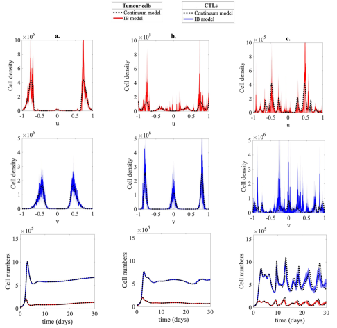
Figure 5: Patterns of phenotypic coevolution between tumour cells and CTLs: impact of the parameter $\eta$. Top panels display the plots of the population density function of tumour cells ($n_{C}$) and bottom panels display the plots of the population density function of CTLs ($n_{T}$) of the individual-based model (solid, coloured lines) and continuum model (dashed, black lines) at the end of numerical simulations (i.e. at $t=30$) when condition (4.10) is satisfied and progressively smaller values of $\eta$ are considered – i.e. $\eta=1$ (panels a.), $\eta=0.6$ (panels b.) and $\eta=0.2$ (panels c.). All the other parameters are as in Table 1 with $\gamma=1$ and $\theta_{C}=\theta_{T}=0.7$. Bottom panels display the corresponding plots of the time evolution of the total number of tumour cells ($\rho_{C}$) and CTLs ($\rho_{T}$). Initial conditions (5.1) and (5.2) with $a=1$ and $A=5$ were used to carry out numerical simulations. Analogous results were obtained when using different values of the parameter $A$ (results not shown). The results from the individual-based model correspond to the average over five realisations of the underlying random walk and the related variance is displayed by the coloured areas surrounding the curves.

Possible discrepancies between individual-based and continuum models

The results that have been presented so far indicate that there is a good agreement between the results of computational simulations of the individual-based model and the numerical solutions of the corresponding continuum model. However, we expect possible differences between the outputs of the two models to emerge in the presence of lower tumour cell numbers, which may lead to more pronounced demographic stochasticity, and less regular multi-peaked cell phenotype distributions, which may cause a reduction in the quality of the approximations employed in the formal derivation of the deterministic continuum model from the individual-based model. In order to investigate this, we carried out numerical simulations of the two models for choices of parameter values such that condition (4.10) holds, evolution towards relatively small tumour cell numbers occurs, and less regular cell phenotype distributions with multiple peaks emerge (see caption of Figure 6 for more details). The results obtained are summarised by the plots in Figure 6, which show that the individual-based model predicts eradication of the tumour cell population, whereas the continuum model predicts coexistence between tumour cells and CTLs.

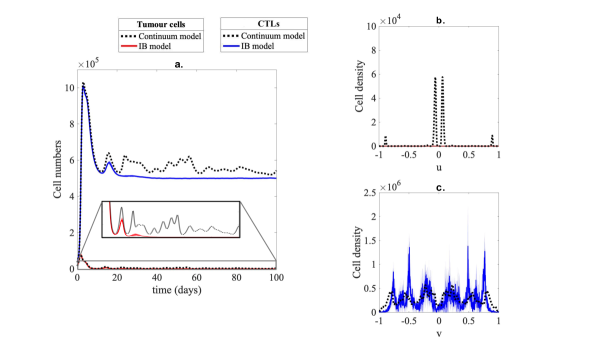
Figure 6: Possible discrepancies between individual-based and continuum models. Panel a. displays the plot of the time evolution of the total number of tumour cells ($\rho_{C}$) and CTLs ($\rho_{T}$) of the individual-based model (solid, coloured lines) and the continuum model (dashed, black lines) when condition (4.10) holds, evolution towards relatively small tumour cell numbers occurs, and the parameter $\eta$ is sufficiently small so that less regular multi-peaked cell phenotype distributions emerge – i.e. $\alpha_{T}=0.5$/day, $\mu_{T}=2\times 10^{-6}\mu l$/day, $\gamma=1.1$, $\eta=0.1$, and all the other parameters as in Table 1 with $\theta_{C}=\theta_{T}=1.8$. The plots in panels b. and c. display the corresponding population density functions of tumour cells ($n_{C}$) and CTLs ($n_{T}$) of the individual-based model (solid, coloured lines) and of the continuum model (dashed, black lines) at the end of simulations (i.e. at $t=t_{f}=100$). Initial conditions (5.1) and (5.2) with $a=1$ and $A=5$ were used to carry out numerical simulations. Analogous results were obtained when using different values of the parameter $A$ (results not shown). The results from the individual-based model correspond to the average over five realisations and the related variance is displayed by the coloured areas surrounding the curves.

6 Discussion, conclusions and research perspectives

Discussion and conclusions

We developed an individual-based model for the coevolutionary dynamics between tumour cells and CD8+ cytotoxic T lymphocytes that takes into account the selectivity of antigen-specific immunity. We formally derived the deterministic continuum counterpart of such an individual-based model, and we integrated the results of numerical simulations of the two models with the results of steady-state and linear-stability analyses of the continuum model equations.

The results presented in this study shed light on the way in which different parameters shape the coevolutionary dynamics between tumour cells and CD8+ cytotoxic T lymphocytes. In particular, we demonstrated that, ceteris paribus, higher values of the TCR-tumour antigen binding affinity (i.e. the parameter $\gamma$ in the model) promote the eradication of tumour cells by CTLs, while lower values facilitate the coexistence between tumour cells and CTLs. Specifically, progressively reducing the TCR-tumour antigen binding affinity brings about the emergence of: hot tumour-like scenarios, which are characterised by a large number of in situ CTLs and a low number of tumour cells, and thus represent a more fertile ground for anticancer therapeutic intervention; altered tumour-like scenarios, which reflect the intrinsic ability of the immune system to effectively mount a CTL-mediated immune response and the ability of tumour cells to partially escape such a response; cold tumour-like scenarios, which are characterised by an insufficient number of in situ CTLs and are invariably associated with poor prognosis [37]. This classification of tumours is also supported by experimental works showing that in situ immune reaction might be the strongest parameter influencing clinical outcome, regardless of the local tumour extension and its spread to lymph nodes [82, 38, 39]. Moreover, our findings support the idea that TCR-tumour antigen binding affinity may be a good intervention target for immunotherapy that aims to turn cold or altered tumours into hot ones by enhancing CTL response. In this regard, our findings are in agreement with the conclusions of previous experimental articles indicating that a strong binding affinity of T cells to tumour antigens may play a key role in the overall immune response to the disease [45].In particular, in altered tumours, increasing antigenicity, via the removal of co-inhibitory signals and/or the supply of co-stimulatory signals [39, 104], may enhance in situ CTLs activity, and has proven to be effective in the treatment of advanced-stage melanoma [107], renal cell carcinoma [80] and non-small cell lung cancer [51]. In cold tumours, a proposed approach to overcome the lack of a pre-existing immune response consists in combining a priming therapy that boosts CTL responses with the removal of co-inhibitory signals through approaches such as immune checkpoint [37]. The therapeutic success achieved by combining immune checkpoint therapy with chemotherapy in metastatic NSCLC has demonstrated the potential strength of this dual approach [40].

Moreover, the results presented here indicate that the affinity range of TCRs (i.e. the parameter $\eta$ in the model), the selectivity of clonal competition amongst tumour cells (i.e. the inverse of the parameter $\theta_{C}$ in the model) and the selectivity of self-regulation mechanisms acting on CD8+ cytotoxic T lymphocytes (i.e. the inverse of the parameter $\theta_{T}$ in the model) play a pivotal role in the formation of patterns of phenotypic coevolution, which create the substrate for the emergence of less regular cell phenotype distributions with multiple peaks. Such patterns are underpinned by some form of immunoediting whereby the population of CTLs evolves and continuously adapts its receptor repertoire in order to recognise and effectively eliminate tumour cells and, in turn, the antigen-specific selective pressure exerted by CTLs leads to the selection of those tumour clones that are able to evade immune recognition [31]. The adaptability of tumour cells and CTLs and the selective pressure they mutually exert on each other during cancer development are emerging as crucial factors in determining cancer evolutionary trajectories. This has been shown in the context of chronic lymphocytic leukemia [85] and other cancer types, as reviewed in [44]. Our results offer also a theoretical basis for the development of anti-cancer therapy aiming at engineering TCRs so as to shape their affinity for cancer targets [12, 22, 64, 111] and adaptive therapy aiming at altering intratumour clonal competition [42, 103], in order to control the coevolutionary dynamics between tumour cells and CD8+ cytotoxic T lymphocytes. In this respect, one of the best known treatment based on engineering specific TCRs is based on CAR-T cells [102], which confer CTLs the ability to target specific antigens. It has been demonstrated that this therapeutic strategy has several potential advantages over conventional therapies, including specificity, rapidity, high success rate and long-lasting effects [55, 46].

The good agreement between the results of numerical simulations of the individual-based and continuum models, along with the quantitative information given by (4.9) and (4.11) and the precise conditions given by (4.20) and (4.27), testifies to the robustness of the biological insight gained in this work. We also showed that possible differences between cell dynamics produced by the individual-based and continuum models can emerge under parameter settings that correspond to less regular cell phenotype distributions and more pronounced demographic stochasticity. In fact, these cause a reduction in the quality of the approximations employed in the formal derivation of the deterministic continuum model from the individual-based model (cf. Appendix A). This demonstrates the importance of integrating individual-based and continuum approaches when considering mathematical models for tumour-immune competition.

Research perspectives

From a mathematical point of view, we plan to carry out a systematic investigation of the conditions on the affinity range of TCRs that may lead to the emergence of oscillations in cell numbers observed in the numerical simulations presented in this work. Moreover, from a modelling point of view, our individual-based modelling framework for the coevolutionary dynamics between tumour cells and CD8+ cytotoxic T lymphocytes, along with the formal derivation of the corresponding continuum model, can be developed further in several ways. For instance, a myriad of immunosuppressive strategies, the so-called immune checkpoints, help tumour cells acquiring features that enable them to evade immune detection, which may ultimately induce the exhaustion of CTLs in the tumour micro-environment, which impairs the immune response. The modelling approach presented here does not capture this aspect. However, exhaustion mechanisms could be incorporated into the individual-based model by, for example, allowing CTLs to enter a suppressed state (i.e. CTLs would become exhausted and thus would no longer able to eliminate tumour cells). In the continuum model, this would result in the presence of an additional loss term in the IDE (3.3)₂ along with a third equation for the dynamics of exhausted CTLs. Another track to follow to further enrich our model would be to include a spatial structure, for instance by embedding the tumour cells in the geometry of a solid tumour, and to take explicitly into account the effect of both spatial and antigen-specific interactions between tumour cells and CTLs, as similarly done in [57, 71, 72]. Including a spatial structure would make it possible, inter alia, to introduce a more precise definition of the immune score that incorporates the level of CTL infiltration. Furthermore, at this stage, the mathematical representation of the phenotypic state of tumour cells and CTLs employed in our modelling framework is rather abstract. This might make it difficult to carry out precise quantitative comparisons between the results of numerical simulations and experimental data. This limitation could be overcome by employing a mathematical representation of tumour antigens and TCRs similar to the one that we proposed in [62], whereby a discrete set of tumour antigens that can be recognised by a unique repertoire of TCRs is considered. Finally, it would be interesting to incorporate explicitly into the model the effects of immunotherapeutic agents or other therapeutic agents. These are all lines of research that we will be pursuing in the future.

Funding

E.L. has received funding from the European Research Council (ERC) under the European Union’s Horizon2020 research and innovation programme (grant agreement No 740623). T.L. gratefully acknowledges support from the Italian Ministry of University and Research (MUR) through the grant “Dipartimenti di Eccellenza 2018-2022” (Project no. E11G18000350001) and the PRIN 2020 project (No. 2020JLWP23) “Integrated Mathematical Approaches to Socio–Epidemiological Dynamics” (CUP: E15F21005420006). L.A., E.L. and T.L. gratefully acknowledge support from the CNRS International Research Project “Modélisation de la biomécanique cellulaire et tissulaire” (MOCETIBI).

Appendix A Formal derivation of the continuum model

Using a method analogous to that employed in [6, 18, 89], we show that the PDE-IDE system (3.3) can be formally derived as the appropriate continuum limit of the individual-based model presented in this article.

Substituting definitions (2.9) of ${\rm P}^{b}_{C}$ and ${\rm P}^{q}_{C}$ into the difference equation (3.1)₁ for $n_{C_{i}}^{h}$ and definitions (2.10) of ${\rm P}^{b}_{T}$ and ${\rm P}^{q}_{T}$ into the difference equation (3.1)₂ for $n_{T_{j}}^{h}$ yields

$$\begin{cases}n_{C_{i}}^{h+1}=\left[1+\tau\,\alpha_{C}-\tau\,\left(\mu_{C}\,K_{C_{i}}^{h}+\zeta_{C}\,\gamma\,J_{C_{i}}^{h}\right)\right]\left[\dfrac{\lambda_{C}}{2}\left(n_{C_{i+1}}^{h}+n_{C_{i-1}}^{h}\right)+(1-\lambda_{C})\,n_{C_{i}}^{h}\right],\\ \\ n_{T_{j}}^{h+1}=\left[1+\tau\,\left(\alpha_{T}+\zeta_{T}\,\gamma\,J_{T_{j}}^{h}\right)-\tau\,\mu_{T}\,K_{T_{j}}^{h}\right]\,n_{T_{i}}^{h},\end{cases}$$ (A.1)

where $n_{C_{i}}^{h}\equiv n_{C}(u_{i},t_{h})$ with $(u_{i},t_{h})\in\mathcal{I}\times(0,t_{f}]$ and $n_{T_{j}}^{h}\equiv n_{T}(v_{j},t_{h})$ with $(v_{j},t_{h})\in\overline{\mathcal{I}}\times(0,t_{f}]$. Using the fact that the following relations hold for $\tau$ and $\chi$ sufficiently small

$$t_{h}\approx t,\quad t_{h+1}\approx t+\tau,\quad u_{i}\approx u,\quad u_{i\pm 1}\approx u\pm\chi,\quad v_{j}\approx v,$$

$$n_{C_{i}}^{h}\approx n_{C}(u,t),\quad n_{C_{i}}^{h+1}\approx n_{C}(u,t+\tau),\quad n_{C_{i\pm 1}}^{h}\approx n_{C}(u\pm\chi,t),\quad\rho_{C}^{h}\approx\rho_{C}(t):=\int_{\mathcal{I}}n_{C}(u,t)\,\mathrm{d}u,$$

$$J_{C_{i}}^{h}\approx J_{C}(u,t):=\int_{\mathcal{I}}g(u,v;\eta)\,n_{T}(v,t)\,\mathrm{d}v,\quad K_{C_{i}}^{h}\approx K_{C}(u,t):=\int_{\mathcal{I}}g(u,w;\theta_{C})\,n_{C}(w,t)\,\mathrm{d}w,$$

$$n_{T_{j}}^{h}\approx n_{T}(v,t),\quad n_{T_{j}}^{h+1}\approx n_{T}(v,t+\tau),\quad\rho_{T}^{h}\approx\rho_{T}(t):=\int_{\mathcal{I}}n_{T}(v,t)\,\mathrm{d}v,$$

$$J_{T_{j}}^{h}\approx J_{T}(v,t):=\int_{\mathcal{I}}g(v,u;\eta)\,n_{C}(u,t)\,\mathrm{d}u,\quad K_{T_{j}}^{h}\approx K_{T}(v,t):=\int_{\mathcal{I}}g(v,w;\theta_{T})\,n_{T}(w,t)\,\mathrm{d}w,$$

where the function $g$ is defined via (2.6), the system of equations (A.1) can be formally rewritten in the approximate form

$$\begin{cases}n_{C}(u,t+\tau)=\Big{[}1+\tau\,R_{C}(K_{C}(u,t),J_{C}(u,t))\Big{]}\times\\ \qquad\qquad\qquad\qquad\qquad\qquad\times\,\left[\dfrac{\lambda_{C}}{2}\left(n_{C}(u+\chi,t)+n_{C}(u-\chi,t)\right)+(1-\lambda_{C})\,n_{C}(u,t)\right],\\ \\ n_{T}(v,t+\tau)=\Big{[}1+\tau\,R_{T}(K_{T}(v,t),J_{T}(v,t))\Big{]}\,n_{T}(v,t),\end{cases}$$ (A.2)

where $u\in\mathcal{I}$, $v\in\overline{\mathcal{I}}$ and $t\in(0,t_{f}]$. Here,

$$R_{C}(K_{C},J_{C}):=\alpha_{C}-\Big{(}\mu_{C}\,K_{C}+\zeta_{C}\,\gamma\,J_{C}\Big{)},\quad R_{T}(K_{T},J_{T}):=\Big{(}\alpha_{T}+\zeta_{T}\,\gamma\,J_{T}\Big{)}-\mu_{T}\,K_{T}.$$ (A.3)

If the function $n_{C}(u,t)$ is twice continuously differentiable with respect to the variable $u$, for $\chi$ sufficiently small we can use the Taylor expansions

$$n_{C}(u\pm\chi,t)=n_{C}(u,t)\pm\chi\partial_{u}n_{C}(u,t)+\frac{\chi^{2}}{2}\partial^{2}_{uu}n_{C}(u,t)+h.o.t.\ .$$ (A.4)

Substituting the Taylor expansions (A.4) into equation (A.2)₁ for $n_{C}(u,t+\tau)$, after a little algebra we find

$$\begin{cases}\dfrac{n_{C}(u,t+\tau)-n_{C}(u,t)}{\tau}-\dfrac{\lambda_{C}\chi^{2}}{2\tau}\partial^{2}_{uu}n_{C}(u,t)=R_{C}(K_{C}(u,t),J_{C}(u,t))\,n_{C}(u,t)+\\ \qquad\qquad\qquad\qquad\qquad\qquad\qquad\qquad\qquad\qquad+\,\dfrac{\lambda_{C}\chi^{2}}{2}\,R_{C}(K_{C}(u,t),J_{C}(u,t))\,\partial^{2}_{uu}n_{C}(u,t)+h.o.t.\,,\\ \\ \dfrac{n_{T}(v,t+\tau)-n_{T}(v,t)}{\tau}=R_{T}(K_{T}(v,t),J_{T}(v,t))\,n_{T}(v,t).\end{cases}$$

If, in addition, the functions $n_{C}(u,t)$ and $n_{T}(v,t)$ are continuously differentiable with respect to the variable $t$, letting $\tau\to 0$ and $\chi\to 0$ in such a way that condition (3.2) is met, from the latter system of equations we formally obtain

$$\begin{cases}\partial_{t}n_{C}(u,t)-\beta_{C}\partial^{2}_{uu}n_{C}(u,t)=R_{C}(K_{C},J_{C})\,n_{C}(u,t),\quad(u,t)\in\mathcal{I}\times(0,t_{f}],\\ \\ \partial_{t}n_{T}(v,t)=R_{T}(K_{T},J_{T})\,n_{T}(v,t),\quad(v,t)\in\overline{\mathcal{I}}\times(0,t_{f}].\end{cases}$$

Substituting definitions (A.3) of $R_{C}(K_{C},J_{C})$ and $R_{T}(K_{T},J_{T})$ into the above system of equations gives the PDE-IDE system (3.3). Finally, the no-flux boundary conditions (3.4) follow from the fact that the attempted phenotypic variation of a tumour cell is aborted if it requires moving into a phenotypic state that does not belong to the interval $\overline{\mathcal{I}}$.

Appendix B Details of numerical simulations of the continuum model

To construct numerical solutions of the PDE-IDE system (3.3) subject both to the no-flux boundary conditions (3.4) and to the initial condition  (5.2), we use a uniform discretisation of step $\Delta x=0.0013$ of the interval $\overline{\mathcal{I}}=[-L,L]$ as the computational domain of the independent variables $u$ and $v$, and a uniform discretisation of step $\Delta t=0.05$ of the time interval $(0,t_{f}]$.

We construct numerical solutions of the non-local PDE (3.3)₁ for $n_{C}$ using a time-splitting approach, which is based on the idea of decomposing the original problem into simpler subproblems that are then sequentially solved at each time-step using an explicit Euler method with step $\Delta t$. This leads to the following time-dicretisation of the PDE-IDE system (3.3) subject to the Neumann boundary conditions (3.4):

$$\begin{cases}n_{C}^{k+\frac{1}{2}}(u)=n_{C}^{k}(u)+\Delta t\,R_{C}(K_{C}^{k}(u),J_{C}^{k}(u))\,n_{C}^{k}(u),\quad u\in[-L,L],\\ \\ n_{C}^{k+1}(u)=n_{C}^{k+\frac{1}{2}}(u)+\Delta t\,\beta_{C}\,\partial^{2}_{uu}n_{C}^{k+\frac{1}{2}}(u),\quad u\in(-L,L),\\ \\ \partial_{u}n_{C}^{k+1}(u)=0,\quad u\in\{-L,L\}\\ \\ n_{T}^{k+1}(v)=n_{T}^{k}(v)+\Delta t\,R_{T}(K_{T}^{k}(v),J_{T}^{k}(v))\,n_{T}^{k}(v),\quad v\in[-L,L],\end{cases}$$ (B.1)

where

$$R_{C}(K_{C}^{k},J_{C}^{k}):=\alpha_{C}-\mu_{C}K_{C}^{k}-\zeta_{C}\gamma J_{C}^{k},\quad R_{T}(K_{T}^{k},J_{T}^{k}):=\alpha_{T}-\mu_{T}K_{T}^{k}-\zeta_{T}\gamma J_{T}^{k}.$$

The system of equations (B.1) is numerically solved using a three-point finite difference explicit scheme for the diffusion term [63] and an implicit-explicit finite difference scheme for the remaining terms [66, 69], which leads to the following system of equations

$$\begin{cases}n_{Ci}^{k+\frac{1}{2}}=n_{Ci}^{k}\dfrac{1+\Delta t\,R_{C}(K_{Ci}^{k},J_{Ci}^{k})_{+}}{1+\Delta t\,R_{C}(K_{Ci}^{k},J_{Ci}^{k})_{-}},\quad u_{i}\in[-L,L],\\ \\ n_{Ci}^{k+1}=n_{Ci}^{k+\frac{1}{2}}+\beta_{C}\Delta t\dfrac{n_{Ci+1}^{k+\frac{1}{2}}-2n_{Ci}^{k+\frac{1}{2}}+n_{Ci-1}^{k+\frac{1}{2}}}{\Delta x^{2}},\quad u_{i}\in(-L,L),\\ \\ n_{Ci}^{k+1}=n_{Ci-1}^{k+1},\quad u_{i}\in\{-L,L\},\\ \\ n_{Tj}^{k+1}=n_{Tj}^{k}\dfrac{1+\Delta t\,R_{T}(K_{Tj}^{k},J_{Tj}^{k})_{+}}{1+\Delta t\,R_{T}(K_{Tj}^{k},J_{Tj}^{k})_{-}},\quad v_{j}\in[-L,L].\end{cases}$$

Here, $R_{C}(\cdot,\cdot)_{+}$ and $R_{T}(\cdot,\cdot)_{+}$ are the positive parts of $R_{C}(\cdot,\cdot)$ and $R_{T}(\cdot,\cdot)$, while $R_{C}(\cdot,\cdot)_{-}$ and $R_{T}(\cdot,\cdot)_{-}$ are the negative parts of $R_{C}(\cdot,\cdot)$ and $R_{T}(\cdot,\cdot)$. Moreover,

$$K_{C_{i}}^{k}=\sum_{q}g(u_{i},u_{q};\theta_{C})\,n_{Cq}^{k}\,\Delta x,\qquad K_{T_{j}}^{h}=\sum_{q}g(v_{j},v_{q};\theta_{T})\,n_{Tq}^{k}\,\Delta x$$

and

$$J_{C_{i}}^{h}=\sum_{j}g(u_{i},v_{j};\eta)\,n_{Tj}^{k}\,\Delta x,\qquad J_{T_{j}}^{h}=\sum_{i}g(v_{j},u_{i};\eta)\,n_{Ci}^{k}\,\Delta x.$$

Given the values of the parameter $\tau$, $\chi$ and $\lambda_{C}$ of the individual-based model, the value of the parameter $\beta_{C}$ is defined so that condition (3.2) is met. The other parameter values are chosen to be coherent with those used to carry out numerical simulations of the individual-based model, which are specified in the main body of the paper.

Appendix C Supplementary figures

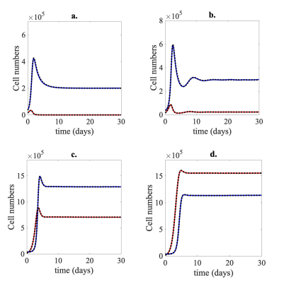
Figure S1: Eradication of tumour cells and emergence of hot tumour-like, altered tumour-like and cold tumour-like scenarios: the case where $a>0$. Panel a. displays the plots of the time evolution of the total number of tumour cells ($\rho_{C}$) and CTLs ($\rho_{T}$) of the individual-based model (solid, coloured lines) and the continuum model (dashed, black lines) when $\gamma$ is high enough that condition (4.20) is satisfied (i.e. condition (4.10) does not hold). Here, $\alpha_{T}=0.5$ and all the other parameters are as in Table 1 with $\gamma=3.5$, $\eta=1.8$ and $\theta_{C}=\theta_{T}=1.8$. Panels b.-d. display similar plots for sufficiently large, intermediate and sufficiently small values of $\gamma$ that satisfy condition (4.10) – i.e. $\gamma=2$ (panel b.), $\gamma=0.3$ (panel c.) and $\gamma=0.12$ (panel d.). All the other parameters are as in Table 1 with $\eta=1.8$ and $\theta_{C}=\theta_{T}=1.8$. Initial conditions (5.1) and (5.2) with $a=1$ and $A=5$ were used to carry out numerical simulations. Analogous results were obtained when using different values of the parameter $A$ (results not shown). The results from the individual-based model correspond to the average over two realisations and the related variance is displayed by the coloured areas surrounding the curves.

References

- Aguadé-Gorgorió and Solé [2020] G. Aguadé-Gorgorió and R. Solé. Tumour neoantigen heterogeneity thresholds provide a time window for combination immunotherapy. Journal of the Royal Society Interface, 17(171):20200736, 2020.
- Al-Tameemi et al. [2012] M. Al-Tameemi, M. Chaplain, and A. d’Onofrio. Evasion of tumours from the control of the immune system: consequences of brief encounters. Biology Direct, 7(1):31, 2012.
- Almuallem et al. [2021] N. Almuallem, D. Trucu, and R. Eftimie. Oncolytic viral therapies and the delicate balance between virus-macrophage-tumour interactions: A mathematical approach. Mathematical Biosciences and Engineering, 18(1):764–799, 2021.
- Altrock et al. [2015] P. M. Altrock, L. L. Liu, and F. Michor. The mathematics of cancer: integrating quantitative models. Nature Reviews Cancer, 15(12):730–745, 2015.
- Angell and Galon [2013] H. Angell and J. Galon. From the immune contexture to the Immunoscore: the role of prognostic and predictive immune markers in cancer. Current Opinion in Immunology, 25(2):261–267, 2013.
- Ardaševa et al. [2020] A. Ardaševa, A. R. Anderson, R. A. Gatenby, H. M. Byrne, P. K. Maini, and T. Lorenzi. Comparative study between discrete and continuum models for the evolution of competing phenotype-structured cell populations in dynamical environments. Physical Review E, 102(4):042404, 2020.
- Atsou et al. [2020] K. Atsou, F. Anjuère, V. M. Braud, and T. Goudon. A size and space structured model describing interactions of tumor cells with immune cells reveals cancer persistent equilibrium states in tumorigenesis. Journal of Theoretical Biology, 490:110163, 2020.
- Balachandran et al. [2017] V. P. Balachandran, M. Łuksza, J. N. Zhao, V. Makarov, J. A. Moral, R. Remark, B. Herbst, G. Askan, U. Bhanot, Y. Senbabaoglu, et al. Identification of unique neoantigen qualities in long-term survivors of pancreatic cancer. Nature, 551(7681):512–516, 2017.
- Bellomo and Preziosi [2000] N. Bellomo and L. Preziosi. Modelling and mathematical problems related to tumor evolution and its interaction with the immune system. Mathematical and Computer Modelling, 32(3-4):413–452, 2000.
- Biselli et al. [2017] E. Biselli, E. Agliari, A. Barra, F. R. Bertani, A. Gerardino, A. De Ninno, A. Mencattini, D. Di Giuseppe, F. Mattei, G. Schiavoni, et al. Organs on chip approach: a tool to evaluate cancer-immune cells interactions. Scientific Reports, 7(1):1–12, 2017.
- Blattman et al. [2002] J. N. Blattman, R. Antia, D. J. Sourdive, X. Wang, S. M. Kaech, K. Murali-Krishna, J. D. Altman, and R. Ahmed. Estimating the precursor frequency of naive antigen-specific CD8 T cells. The Journal of Experimental Medicine, 195(5):657–664, 2002.
- Border et al. [2019] E. C. Border, J. P. Sanderson, T. Weissensteiner, A. B. Gerry, and N. J. Pumphrey. Affinity-enhanced T-cell receptors for adoptive T-cell therapy targeting MAGE-A10: strategy for selection of an optimal candidate. Oncoimmunology, 8(2):e1532759, 2019.
- Bubba et al. [2020] F. Bubba, T. Lorenzi, and F. R. Macfarlane. From a discrete model of chemotaxis with volume-filling to a generalized Patlak–Keller–Segel model. Proceedings of the Royal Society A, 476(2237):20190871, 2020.
- Campoli and Ferrone [2008] M. Campoli and S. Ferrone. HLA antigen changes in malignant cells: epigenetic mechanisms and biologic significance. Oncogene, 27(45):5869–5885, 2008.
- Cattani et al. [2010] C. Cattani, A. Ciancio, and A. d’Onofrio. Metamodeling the learning–hiding competition between tumours and the immune system: a kinematic approach. Mathematical and Computer Modelling, 52(1):62–69, 2010.
- Chaplain et al. [2020] M. A. Chaplain, T. Lorenzi, and F. R. Macfarlane. Bridging the gap between individual-based and continuum models of growing cell populations. Journal of Mathematical Biology, 80(1-2):343–371, 2020.
- Chisholm et al. [2016a] R. H. Chisholm, T. Lorenzi, and J. Clairambault. Cell population heterogeneity and evolution towards drug resistance in cancer: biological and mathematical assessment, theoretical treatment optimisation. Biochimica et Biophysica Acta (BBA)-General Subjects, 1860(11):2627–2645, 2016a.
- Chisholm et al. [2016b] R. H. Chisholm, T. Lorenzi, L. Desvillettes, and B. D. Hughes. Evolutionary dynamics of phenotype-structured populations: from individual-level mechanisms to population-level consequences. Zeitschrift für angewandte Mathematik und Physik, 67(4):100, 2016b.
- Chisholm et al. [2016c] R. H. Chisholm, T. Lorenzi, and A. Lorz. Effects of an advection term in nonlocal Lotka–Volterra equations. Communications in Mathematical Sciences, 14(4):1181–1188, 2016c.
- Christophe et al. [2015] C. Christophe, S. Müller, M. Rodrigues, A.-E. Petit, P. Cattiaux, L. Dupré, S. Gadat, and S. Valitutti. A biased competition theory of cytotoxic T lymphocyte interaction with tumor nodules. PLoS ONE, 10(3):e0120053, 2015.
- Coulie et al. [2014] P. G. Coulie, B. J. Van den Eynde, P. Van Der Bruggen, and T. Boon. Tumour antigens recognized by T lymphocytes: at the core of cancer immunotherapy. Nature Reviews Cancer, 14(2):135–146, 2014.
- Crean et al. [2020] R. M. Crean, B. J. MacLachlan, F. Madura, T. Whalley, P. J. Rizkallah, C. J. Holland, C. McMurran, S. Harper, A. Godkin, A. K. Sewell, et al. Molecular Rules Underpinning Enhanced Affinity Binding of Human T Cell Receptors Engineered for Immunotherapy. Molecular Therapy-Oncolytics, 18:443–456, 2020.
- de Pillis et al. [2005] L. G. de Pillis, A. E. Radunskaya, and C. L. Wiseman. A validated mathematical model of cell-mediated immune response to tumor growth. Cancer Research, 65(17):7950–7958, 2005.
- de Pillis et al. [2009] L. G. de Pillis, K. Renee Fister, W. Gu, C. Collins, M. Daub, D. Gross, J. Moore, and B. Preskill. Mathematical model creation for cancer chemo-immunotherapy. Computational and Mathematical Methods in Medicine, 10(3):165–184, 2009.
- Delitala and Lorenzi [2013a] M. Delitala and T. Lorenzi. Evolutionary branching patterns in predator-prey structured populations. Discrete & Continuous Dynamical Systems-B, 18(9):2267, 2013a.
- Delitala and Lorenzi [2013b] M. Delitala and T. Lorenzi. Recognition and learning in a mathematical model for immune response against cancer. Discrete & Continuous Dynamical Systems-B, 18(4), 2013b.
- Delitala et al. [2013] M. Delitala, U. Dianzani, T. Lorenzi, and M. Melensi. A mathematical model for immune and autoimmune response mediated by T-cells. Computers & Mathematics with Applications, 66(6):1010–1023, 2013.
- Doerfler and Böhm [2006] W. Doerfler and P. Böhm. DNA methylation: development, genetic disease and cancer, volume 310. Springer Science & Business Media, 2006.
- d’Onofrio [2008] A. d’Onofrio. Metamodeling tumor–immune system interaction, tumor evasion and immunotherapy. Mathematical and Computer Modelling, 47(5-6):614–637, 2008.
- Duesberg et al. [2000] P. Duesberg, R. Stindl, and R. Hehlmann. Explaining the high mutation rates of cancer cells to drug and multidrug resistance by chromosome reassortments that are catalyzed by aneuploidy. Proceedings of the National Academy of Sciences, 97(26):14295–14300, 2000.
- Dunn et al. [2002] G. P. Dunn, A. T. Bruce, H. Ikeda, L. J. Old, and R. D. Schreiber. Cancer immunoediting: from immunosurveillance to tumor escape. Nature Immunology, 3(11):991–998, 2002.
- Eftimie et al. [2011] R. Eftimie, J. L. Bramson, and D. J. Earn. Interactions between the immune system and cancer: a brief review of non-spatial mathematical models. Bulletin of Mathematical Biology, 73(1):2–32, 2011.
- Eladdadi et al. [2014] A. Eladdadi, P. Kim, and D. Mallet. Mathematical models of tumor-immune system dynamics, volume 107. Springer, 2014.
- Figueredo et al. [2013] G. P. Figueredo, P.-O. Siebers, and U. Aickelin. Investigating mathematical models of immuno-interactions with early-stage cancer under an agent-based modelling perspective. In BMC Bioinformatics, volume 14, pages 1–20. BioMed Central, 2013.
- Frascoli et al. [2014] F. Frascoli, P. S. Kim, B. D. Hughes, and K. A. Landman. A dynamical model of tumour immunotherapy. Mathematical Biosciences, 253:50–62, 2014.
- Gajewski et al. [2017] T. F. Gajewski, L. Corrales, J. Williams, B. Horton, A. Sivan, and S. Spranger. Cancer immunotherapy targets based on understanding the T cell-inflamed versus non-T cell-inflamed tumor microenvironment. In Tumor Immune Microenvironment in Cancer Progression and Cancer Therapy, pages 19–31. Springer, 2017.
- Galon and Bruni [2019] J. Galon and D. Bruni. Approaches to treat immune hot, altered and cold tumours with combination immunotherapies. Nature Reviews Drug Discovery, 18(3):197–218, 2019.
- Galon et al. [2006] J. Galon, A. Costes, F. Sanchez-Cabo, A. Kirilovsky, B. Mlecnik, C. Lagorce-Pagès, M. Tosolini, M. Camus, A. Berger, P. Wind, et al. Type, density, and location of immune cells within human colorectal tumors predict clinical outcome. Science, 313(5795):1960–1964, 2006.
- Galon et al. [2016] J. Galon, B. Fox, C. Bifulco, G. Masucci, T. Rau, G. Botti, F. Marincola, G. Ciliberto, F. Pages, P. Ascierto, et al. Immunoscore and Immunoprofiling in cancer: an update from the melanoma and immunotherapy bridge 2015. Journal of Translational Medicine, 14(273), 2016.
- Gandhi et al. [2018] L. Gandhi, D. Rodríguez-Abreu, S. Gadgeel, E. Esteban, E. Felip, F. De Angelis, M. Domine, P. Clingan, M. J. Hochmair, S. F. Powell, et al. Pembrolizumab plus chemotherapy in metastatic non–small-cell lung cancer. New England journal of medicine, 378(22):2078–2092, 2018.
- Garrod et al. [2012] K. R. Garrod, H. D. Moreau, Z. Garcia, F. Lemaître, I. Bouvier, M. L. Albert, and P. Bousso. Dissecting T cell contraction in vivo using a genetically encoded reporter of apoptosis. Cell Reports, 2(5):1438–1447, 2012.
- Gatenby et al. [2009] R. A. Gatenby, A. S. Silva, R. J. Gillies, and B. R. Frieden. Adaptive therapy. Cancer Research, 69(11):4894–4903, 2009.
- Génieys et al. [2006] S. Génieys, V. Volpert, and P. Auger. Adaptive dynamics: modelling Darwin’s divergence principle. Comptes Rendus Biologies, 329(11):876–879, 2006.
- George and Levine [2021] J. T. George and H. Levine. Implications of tumor–immune coevolution on cancer evasion and optimized immunotherapy. Trends in Cancer, 7(4):373–383, 2021.
- Gerdemann et al. [2011] U. Gerdemann, U. Katari, A. S. Christin, C. R. Cruz, T. Tripic, A. Rousseau, S. M. Gottschalk, B. Savoldo, J. F. Vera, H. E. Heslop, et al. Cytotoxic t lymphocytes simultaneously targeting multiple tumor-associated antigens to treat ebv negative lymphoma. Molecular therapy, 19(12):2258–2268, 2011.
- Gomes-Silva and Ramos [2018] D. Gomes-Silva and C. A. Ramos. Cancer immunotherapy using car-t cells: from the research bench to the assembly line. Biotechnology journal, 13(2):1700097, 2018.
- Griffiths et al. [2020] J. I. Griffiths, P. Wallet, L. T. Pflieger, D. Stenehjem, X. Liu, P. A. Cosgrove, N. A. Leggett, J. A. McQuerry, G. Shrestha, M. Rossetti, et al. Circulating immune cell phenotype dynamics reflect the strength of tumor–immune cell interactions in patients during immunotherapy. Proceedings of the National Academy of Sciences, 117(27):16072–16082, 2020.
- Handel et al. [2020] A. Handel, N. L. La Gruta, and P. G. Thomas. Simulation modelling for immunologists. Nature Reviews Immunology, 20(3):186–195, 2020.
- Hellerstein et al. [1999] M. Hellerstein, M. Hanley, D. Cesar, S. Siler, C. Papageorgopoulos, E. Wieder, D. Schmidt, R. Hoh, R. Neese, D. Macallan, et al. Directly measured kinetics of circulating T lymphocytes in normal and HIV-1-infected humans. Nature Medicine, 5(1):83–89, 1999.
- Hellmann et al. [2016] M. D. Hellmann, C. F. Friedman, and J. D. Wolchok. Combinatorial cancer immunotherapies. Advances in Immunology, 130:251–277, 2016.
- Hellmann et al. [2018] M. D. Hellmann, T.-E. Ciuleanu, A. Pluzanski, J. S. Lee, G. A. Otterson, C. Audigier-Valette, E. Minenza, H. Linardou, S. Burgers, P. Salman, et al. Nivolumab plus ipilimumab in lung cancer with a high tumor mutational burden. New England Journal of Medicine, 378(22):2093–2104, 2018.
- Huang et al. [2017] A. C. Huang, M. A. Postow, R. J. Orlowski, R. Mick, B. Bengsch, S. Manne, W. Xu, S. Harmon, J. R. Giles, B. Wenz, et al. T-cell invigoration to tumour burden ratio associated with anti-PD-1 response. Nature, 545(7652):60, 2017.
- Huang [2013] S. Huang. Genetic and non-genetic instability in tumor progression: link between the fitness landscape and the epigenetic landscape of cancer cells. Cancer and Metastasis Reviews, 32(3-4):423–448, 2013.
- Hughes [1995] B. D. Hughes. Random walks and random environments: random walks, volume 1. Oxford University Press, 1995.
- June et al. [2018] C. H. June, R. S. O’Connor, O. U. Kawalekar, S. Ghassemi, and M. C. Milone. Car t cell immunotherapy for human cancer. Science, 359(6382):1361–1365, 2018.
- Kastritis and Bonvin [2013] P. L. Kastritis and A. M. Bonvin. On the binding affinity of macromolecular interactions: daring to ask why proteins interact. Journal of The Royal Society Interface, 10(79):20120835, 2013.
- Kather et al. [2017] J. N. Kather, J. Poleszczuk, M. Suarez-Carmona, J. Krisam, P. Charoentong, N. A. Valous, C.-A. Weis, L. Tavernar, F. Leiss, E. Herpel, et al. In silico modeling of immunotherapy and stroma-targeting therapies in human colorectal cancer. Cancer Research, 77(22):6442–6452, 2017.
- Kolev [2003] M. Kolev. Mathematical modeling of the competition between acquired immunity and cancer. International Journal of Applied Mathematics and Computer Science, 13:289–296, 2003.
- Konstorum et al. [2017] A. Konstorum, A. T. Vella, A. J. Adler, and R. C. Laubenbacher. Addressing current challenges in cancer immunotherapy with mathematical and computational modelling. Journal of The Royal Society Interface, 14(131):20170150, 2017.
- Kuznetsov and Knott [2001] V. A. Kuznetsov and G. D. Knott. Modeling Tumor Regrowth and Immunotherapy. Mathematical and Computer Modelling, 33(12):1275–1287, 2001.
- Kuznetsov et al. [1994] V. A. Kuznetsov, I. A. Makalkin, M. A. Taylor, and A. S. Perelson. Nonlinear dynamics of immunogenic tumors: parameter estimation and global bifurcation analysis. Bulletin of Mathematical Biology, 56(2):295–321, 1994.
- Leschiera et al. [2022] E. Leschiera, T. Lorenzi, S. Shen, L. Almeida, and C. Audebert. A mathematical model to study the impact of intra-tumour heterogeneity on anti-tumour cd8+ t cell immune response. Journal of Theoretical Biology, page 111028, 2022.
- LeVeque [2007] R. J. LeVeque. Finite difference methods for ordinary and partial differential equations: steady-state and time-dependent problems. SIAM, 2007.
- Li et al. [2019] D. Li, X. Li, W.-L. Zhou, Y. Huang, X. Liang, L. Jiang, X. Yang, J. Sun, Z. Li, W.-D. Han, et al. Genetically engineered T cells for cancer immunotherapy. Signal Transduction and Targeted Therapy, 4(1):1–17, 2019.
- Lin Erickson et al. [2009] A. H. Lin Erickson, A. Wise, S. Fleming, M. Baird, Z. Lateef, A. Molinaro, M. Teboh-Ewungkem, and L. G. de Pillis. A preliminary mathematical model of skin dendritic cell trafficking and induction of T cell immunity. Discrete & Continuous Dynamical Systems - B, 12:323–336, 2009.
- Lorenzi et al. [2015a] T. Lorenzi, R. H. Chisholm, L. Desvillettes, and B. D. Hughes. Dissecting the dynamics of epigenetic changes in phenotype-structured populations exposed to fluctuating environments. Journal of Theoretical Biology, 386:166–176, 2015a.
- Lorenzi et al. [2015b] T. Lorenzi, R. H. Chisholm, M. Melensi, A. Lorz, and M. Delitala. Mathematical model reveals how regulating the three phases of T-cell response could counteract immune evasion. Immunology, 146(2):271–280, 2015b.
- Lorenzi et al. [2019] T. Lorenzi, F. R. Macfarlane, and C. Villa. Discrete and continuum models for the evolutionary and spatial dynamics of cancer: a very short introduction through two case studies. In International Symposium on Mathematical and Computational Biology, pages 359–380. Springer, 2019.
- Lorz et al. [2013] A. Lorz, T. Lorenzi, M. E. Hochberg, J. Clairambault, and B. Perthame. Populational adaptive evolution, chemotherapeutic resistance and multiple anti-cancer therapies. ESAIM: Mathematical Modelling and Numerical Analysis, 47(2):377–399, 2013.
- Łuksza et al. [2017] M. Łuksza, N. Riaz, V. Makarov, V. P. Balachandran, M. D. Hellmann, A. Solovyov, N. A. Rizvi, T. Merghoub, A. J. Levine, T. A. Chan, et al. A neoantigen fitness model predicts tumour response to checkpoint blockade immunotherapy. Nature, 551(7681):517–520, 2017.
- Macfarlane et al. [2018] F. R. Macfarlane, T. Lorenzi, and M. A. Chaplain. Modelling the immune response to cancer: an individual-based approach accounting for the difference in movement between inactive and activated T cells. Bulletin of Mathematical Biology, 80(6):1539–1562, 2018.
- Macfarlane et al. [2019] F. R. Macfarlane, M. A. Chaplain, and T. Lorenzi. A stochastic individual-based model to explore the role of spatial interactions and antigen recognition in the immune response against solid tumours. Journal of Theoretical Biology, 480:43–55, 2019.
- Makaryan et al. [2020] S. Z. Makaryan, C. G. Cess, and S. D. Finley. Modeling immune cell behavior across scales in cancer. Wiley Interdisciplinary Reviews: Systems Biology and Medicine, 12(4):e1484, 2020.
- Mason [1998] D. Mason. A very high level of crossreactivity is an essential feature of the T-cell receptor. Immunology Today, 9:395–404, 1998.
- Mayer et al. [2019] A. Mayer, Y. Zhang, A. S. Perelson, and N. S. Wingreen. Regulation of T cell expansion by antigen presentation dynamics. Proceedings of the National Academy of Sciences, 116(13):5914–5919, 2019.
- Messerschmidt et al. [2016] J. L. Messerschmidt, G. C. Prendergast, and G. L. Messerschmidt. How cancers escape immune destruction and mechanisms of action for the new significantly active immune therapies: Helping nonimmunologists decipher recent advances. The Oncologist, 21(2):233–243, 2016.
- Min [2018] B. Min. Spontaneous T cell proliferation: a physiologic process to create and maintain homeostatic balance and diversity of the immune system. Frontiers in Immunology, 9:547, 2018.
- Mlecnik et al. [2011] B. Mlecnik, M. Tosolini, A. Kirilovsky, A. Berger, G. Bindea, T. Meatchi, P. Bruneval, Z. Trajanoski, W.-H. Fridman, F. Pages, et al. Histopathologic-based prognostic factors of colorectal cancers are associated with the state of the local immune reaction. Journal of Clinical Oncology, 29(6):610–618, 2011.
- Mlecnik et al. [2014] B. Mlecnik, G. Bindea, H. K. Angell, M. S. Sasso, A. C. Obenauf, T. Fredriksen, L. Lafontaine, A. M. Bilocq, A. Kirilovsky, M. Tosolini, et al. Functional network pipeline reveals genetic determinants associated with in situ lymphocyte proliferation and survival of cancer patients. Science Translational Medicine, 6(228):228ra37–228ra37, 2014.
- Motzer et al. [2018] R. J. Motzer, N. M. Tannir, D. F. McDermott, O. A. Frontera, B. Melichar, T. K. Choueiri, E. R. Plimack, P. Barthélémy, C. Porta, S. George, et al. Nivolumab plus ipilimumab versus sunitinib in advanced renal-cell carcinoma. New England Journal of Medicine, 2018.
- Oey and Whitelaw [2014] H. Oey and E. Whitelaw. On the meaning of the word ‘epimutation’. Trends in Genetics, 30(12):519–520, 2014.
- Pagès et al. [2008] F. Pagès, J. Galon, and W. H. Fridman. The essential role of the in situ immune reaction in human colorectal cancer. Journal of leukocyte biology, 84(4):981–987, 2008.
- Phillips [2002] R. E. Phillips. Immunology taught by Darwin. Nature Immunology, 3(11):987–989, 2002.
- Prehn and Main [1957] R. T. Prehn and J. M. Main. Immunity to methylcholanthrene-induced sarcomas. Journal of the National Cancer Institute, 18(6):769–778, 1957.
- Purroy and Wu [2017] N. Purroy and C. J. Wu. Coevolution of leukemia and host immune cells in chronic lymphocytic leukemia. Cold Spring Harbor perspectives in medicine, 7(4):a026740, 2017.
- Schlesinger et al. [2014] K. J. Schlesinger, S. P. Stromberg, and J. M. Carlson. Coevolutionary immune system dynamics driving pathogen speciation. PLoS ONE, 9(7), 2014.
- Segal et al. [2013] B. Segal, V. Volpert, and A. Bayliss. Pattern formation in a model of competing populations with nonlocal interactions. Physica D: Nonlinear Phenomena, 253:12–22, 2013.
- Sigalotti et al. [2004] L. Sigalotti, E. Fratta, S. Coral, S. Tanzarella, R. Danielli, F. Colizzi, E. Fonsatti, C. Traversari, M. Altomonte, and M. Maio. Intratumor heterogeneity of cancer/testis antigens expression in human cutaneous melanoma is methylation-regulated and functionally reverted by 5-Aza-2‘-deoxycytidine. Cancer Research, 64(24):9167–9171, 2004.
- Stace et al. [2020] R. E. Stace, T. Stiehl, M. A. Chaplain, A. Marciniak-Czochra, and T. Lorenzi. Discrete and continuum phenotype-structured models for the evolution of cancer cell populations under chemotherapy. Mathematical Modelling of Natural Phenomena, 15:14, 2020.
- Stockinger et al. [2004] B. Stockinger, T. Barthlott, and G. Kassiotis. The concept of space and competition in immune regulation. Immunology, 111(3):241, 2004.
- Stone et al. [2009] J. D. Stone, A. S. Chervin, and D. M. Kranz. T-cell receptor binding affinities and kinetics: impact on T-cell activity and specificity. Immunology, 126(2):165–176, 2009.
- Stromberg and Antia [2012] S. P. Stromberg and R. Antia. On the role of CD8 T cells in the control of persistent infections. Biophysical Journal, 103(8):1802–1810, 2012.
- Stromberg and Carlson [2006] S. P. Stromberg and J. Carlson. Robustness and fragility in immunosenescence. PLoS Computational Biology, 2(11), 2006.
- Stromberg and Carlson [2013] S. P. Stromberg and J. M. Carlson. Diversity of T-cell responses. Physical Biology, 10(2):025002, 2013.
- Takayanagi and Ohuchi [2001] T. Takayanagi and A. Ohuchi. A mathematical analysis of the interactions between immunogenic tumor cells and cytotoxic T lymphocytes. Microbiology and Immunology, 45(10):709–715, 2001.
- Tan et al. [2015] M. Tan, A. Gerry, J. Brewer, L. Melchiori, J. S. Bridgeman, A. Bennett, N. Pumphrey, B. Jakobsen, D. Price, K. Ladell, et al. T cell receptor binding affinity governs the functional profile of cancer-specific cd8+ t cells. Clinical & Experimental Immunology, 180(2):255–270, 2015.
- Tian et al. [2017] C. Tian, Z. Ling, and L. Zhang. Nonlocal interaction driven pattern formation in a prey–predator model. Applied Mathematics and Computation, 308:73–83, 2017.
- Troy and Shen [2003] A. E. Troy and H. Shen. Cutting edge: homeostatic proliferation of peripheral T lymphocytes is regulated by clonal competition. The Journal of Immunology, 170(2):672–676, 2003.
- Tumeh et al. [2014] P. C. Tumeh, C. L. Harview, J. H. Yearley, I. P. Shintaku, E. J. Taylor, L. Robert, B. Chmielowski, M. Spasic, G. Henry, V. Ciobanu, et al. PD-1 blockade induces responses by inhibiting adaptive immune resistance. Nature, 515(7528):568–571, 2014.
- Urosevic et al. [2005] M. Urosevic, B. Braun, J. Willers, G. Burg, and R. Dummer. Expression of melanoma-associated antigens in melanoma cell cultures. Experimental Dermatology, 14(7):491–497, 2005.
- Walker and Enderling [2016] R. Walker and H. Enderling. From concept to clinic: Mathematically informed immunotherapy. Current Problems in Cancer, 40(1):68–83, 2016.
- Wang and Rivière [2016] X. Wang and I. Rivière. Clinical manufacturing of car t cells: foundation of a promising therapy. Molecular Therapy-Oncolytics, 3:16015, 2016.
- West et al. [2020] J. West, L. You, J. Zhang, R. A. Gatenby, J. S. Brown, P. K. Newton, and A. R. Anderson. Towards multidrug adaptive therapy. Cancer Research, 80(7):1578–1589, 2020.
- Whiteside et al. [2016] T. L. Whiteside, S. Demaria, M. E. Rodriguez-Ruiz, H. M. Zarour, and I. Melero. Emerging opportunities and challenges in cancer immunotherapy. Clinical Cancer Research, 22(8):1845–1855, 2016.
- Wilkie [2013] K. P. Wilkie. A review of mathematical models of cancer–immune interactions in the context of tumor dormancy. Systems Biology of Tumor Dormancy, pages 201–234, 2013.
- Wilkie and Hahnfeldt [2013] K. P. Wilkie and P. Hahnfeldt. Mathematical models of immune-induced cancer dormancy and the emergence of immune evasion. Interface Focus, 3(4):20130010, 2013.
- Wolchok et al. [2017] J. D. Wolchok, V. Chiarion-Sileni, R. Gonzalez, P. Rutkowski, J.-J. Grob, C. L. Cowey, C. D. Lao, J. Wagstaff, D. Schadendorf, P. F. Ferrucci, et al. Overall survival with combined nivolumab and ipilimumab in advanced melanoma. New England Journal of Medicine, 377(14):1345–1356, 2017.
- Wooldridge et al. [2012] L. Wooldridge, J. Ekeruche-Makinde, H. a. Van Den Berg, A. Skowera, J. J. Miles, M. P. Tan, G. Dolton, M. Clement, S. Llewellyn-Lacey, D. A. Price, et al. A single autoimmune T cell receptor recognizes more than a million different peptides. Journal of Biological Chemistry, 287(2):1168–1177, 2012.
- Yu et al. [2018] Y. Yu, X. Ma, R. Gong, J. Zhu, L. Wei, and J. Yao. Recent advances in CD8 regulatory T cell research. Oncology Letters, 15(6):8187–8194, 2018.
- Zhang et al. [2007] P. Zhang, A. L. Côté, V. C. de Vries, E. J. Usherwood, and M. J. Turk. Induction of postsurgical tumor immunity and t-cell memory by a poorly immunogenic tumor. Cancer research, 67(13):6468–6476, 2007.
- Zhao et al. [2021] Q. Zhao, Y. Jiang, S. Xiang, P. J. Kaboli, J. Shen, Y. Zhao, X. Wu, F. Du, M. Li, C. H. Cho, et al. Engineered TCR-T Cell Immunotherapy in Anticancer Precision Medicine: Pros and Cons. Frontiers in Immunology, 12:812, 2021.
- Zinkernagel et al. [1996] R. M. Zinkernagel, M. F. Bachmann, T. M. Kündig, S. Oehen, H. Pirchet, and H. Hengartner. On immunological memory. Annual Review of Immunology, 14(1):333–367, 1996.