The First Detection of CH₂CN in a Protoplanetary Disk

Abstract

We report the first detection of the molecule cyanomethyl, CH2CN, in a protoplanetary disk. Until now, CH2CN had only been observed at earlier evolutionary stages, in the giant molecular clouds TMC-1 and Sgr 2, and the prestellar core L1544. We detect six transitions of ortho-CH2CN towards the disk around nearby T Tauri star TW Hya. An excitation analysis reveals that the disk-averaged column density, $N$, for ortho-CH2CN is $(6.3\pm 0.5)\times 10^{12}$ cm^-2, which is rescaled to reflect a 3:1 ortho-para ratio, resulting in a total column density, $N_{\rm tot}$, of $(8.4\pm 0.7)\times 10^{12}$ cm^-2. We calculate a disk-average rotational temperature, $T_{\rm{rot}}$ = $40\pm 5$ K, while a radially resolved analysis shows that $T_{\rm{rot}}$ remains relatively constant across the radius of the disk. This high rotation temperature suggests that in a static disk and if vertical mixing can be neglected, CH2CN is largely formed through gas-phase reactions in the upper layers of the disk, rather than solid-state reactions on the surface of grains in the disk midplane. The integrated intensity radial profiles show a ring structure consistent with molecules such as CN and DCN. We note that this is also consistent with previous lower-resolution observations of centrally peaked CH₃CN emission towards the TW Hya disks, since the observed emission gap disappears when convolving our observations with a larger beam size. We obtain a CH2CN/CH3CN ratio ranging between 4 and 10. This high CH2CN/CH3CN is reproduced in a representative chemical model of the TW Hya disk that employs standard static disk chemistry model assumptions, i.e. without any additional tuning.

modules = all, formula = mhchem

1 Introduction

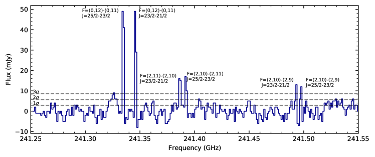
Figure 1: Spectrum of the observed CH2CN transitions. The 6 brightest peaks are shown with their quantum numbers. The noise is calculated to be 2.9 mJy, with the horizontal dashed lines showing 1, 2 and $3~{}\sigma$ levels.

The composition of planets, and therefore their suitability to host biological life, is largely dictated by the physical structure and chemical composition of ice and dust grains in the protoplanetary disks surrounding young stars (e.g., Nomura et al., 2016; Andrews et al., 2012). Nitriles are of specific interests since they have, in fact, often been identified as key precursors in the synthesis of RNA and amino acids (Powner et al., 2009; Patel et al., 2015). Observations of comets and meteors reveal that molecules such as HCN and CH3CN were present in the chemical environment of our early Solar Nebula, and were likely available for prebiotic reactions (Mumma & Charnley, 2011; Altwegg et al., 2020). Nitrile existence in both our early Solar system and in the disks of young stars has implications for our understanding of the trajectory of the organic chemistry as it evolves during planet formation. This is important to estimate the organic inventory on newly-formed planets and to determine what factors contribute to the chemical habitability of nascent planets (Bergner et al., 2018).

HCN and CN were among the first compounds to be observed in a protoplanetary disk, and since their detection in 1997 over 25 new species have been identified in disks (Kastner et al., 1997; McGuire, 2018). However, it was not until the advent of ALMA that more complex molecules such as acetonitrile, CH3CN, and methanol, CH3OH, were observed (Öberg et al., 2015; Walsh et al., 2016). Other nitriles that have been detected include HNC and cyanopolyyne, HC3N, as well as various isotopologues of HCN and CN, including H¹³CN, HC¹⁵N, DCN and C¹⁵N (Dutrey et al., 1997; Chapillon et al., 2012; Guzmán et al., 2015; Qi et al., 2003; Hily-Blant et al., 2017). Together these nitriles constitute a substantial fraction of the detected organics in disks, which points to an interesting variations in chemical composition at different stages of a star’s life: the early stellar stages seem to have significantly less oxygen-rich species than protoplantary disks (Oberg & Bergin, 2020). This could be as a result of the oxygen being locked up in molecules such as CO and H2O and thus unavailable for chemistry, or of a generally oxygen-poor grain-surface chemistry (Oberg & Bergin, 2020).

The formation of complex organic molecules (COMs) in protoplanetary disks can happen via two distinct pathways: through grain-surface or gas-phase reactions. Freeze-out reactions on the surface of grains seem to be the greatest contributors to the abundance of COMs in disks, and they involve the absorption of UV radiation from both the central star and the interstellar radiation field (ISRF), formation of radicals and subsequent rearrangement into more complex organics (Oberg, 2016). Gas-phase reactions are dominated by a variety of reactions including radiative association (molecules collide and emit a photon), neutral-neutral and neutral-ion reactions and dissociative recombination, where a positive ion recombines with an electron. This was found to be the main reaction pathway for the formation of CH3CN in TW Hya and of CH2CN in the protostellar core L1544 (Loomis et al., 2018a; Vastel et al., 2015). Whether this is also the case for CH2CN in disks has not previously been possible to evaluate since there have been no reported observations of this molecule.

In this paper, we report the first observation of the molecule CH2CN (in its ortho state) in a protoplanetary disk, specifically in the disk around the nearby T Tauri star TW Hya. This molecule has previously been observed in diffuse molecular clouds SgrB2 and TMC-1, in the pre-stellar core L1544, and in the circumstellar envelope surrounding the star IRC +10216 but never in a protoplanetary disk (Vastel et al., 2015; Irvine et al., 1988; Agúndez et al., 2008). Liszt et al. (2018) also attempted to place upper limits on the abundance of CH2CN in diffuse molecular gas. TW Hya is a $\sim 0.8M_{\odot}$ solar-like T Tauri star that is often used in astrochemical observations because of its proximity (60.1 pc Bailer-Jones et al., 2018) and its face-on orientation, $i\approx 5\arcdeg$, which allows for easier interpretation of the data. The details of the detection, the data reduction and the observational results are outlined in §2. In §3, we proceed by using a disk-averaged rotational diagram analysis to obtain the total column density for ortho-CH2CN and an excitation temperature. We also perform a radially resolved analysis to obtain radial profiles for both these parameters. In §4 we compare our findings to a chemical model of TW Hya, which we use to complement our discussion of the chemistry of both CH3CN and CH2CN. Finally, we present a summary of our findings in §5.

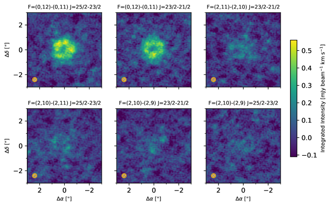
Figure 2: Integrated intensity images of individual observed transitions. All the panels share the same intensity scale. The synthesised beam is shown in the bottom left corner. We find $\sigma$ to be $0.06~{}{\rm mJy~{}beam}^{-1}~{}{\rm km~{}s}^{-1}$.

2 Observations

These observations were taken as part of an ALMA project 2018.A.00021 (PI: Teague), designed to observe ¹²CO (2-1), CS (5-4) and CN (2-1) emission at high spatial and spectral resolution from the disk around TW Hya (J2000 R.A. 11h01m51.905s, Decl. -34d42m17.03s). The correlator set-up included a single frequency divided mode (FDM) window centered on 241.5 GHz to provide continuum on which to self-calibrate. In this window six strong emission lines were detected and identified as CH2CN lines, and a single C^34S line.

2.1 Data Reduction

Table 1: Observed CH₂CN Transitions

$N^{\prime}-N^{\prime\prime}$	$K_{a}$	$K_{c}$	$J^{\prime}-J^{\prime\prime}$	$\nu_{0}$	$g_{u}$	$A_{ul}$	$S_{\rm ij}\mu^{2}$	$E_{\rm upper}$	Int. Flux Density
				(GHz)		$({\rm s}^{-1})$	$({\rm D}^{2})$	(K)	$({\rm mJy~{}km~{}s}^{-1})$
12-11	0 - 0	12 - 11	25/2 - 23/2	241.3335423	234	$9.62\times 10^{-4}$	1376.0	75	$126.1\pm 6.0$
12-11	0 - 0	12 - 11	23/2 - 21/2	241.3458390	216	$9.59\times 10^{-4}$	1265.6	75	$109.3\pm 6.0$
12-11	2 - 2	11 - 10	23/2 - 21/2	241.3860255	216	$9.33\times 10^{-4}$	1230.5	128	$43.4\pm 6.0$
12-11	2 - 2	11 - 10	25/2 - 23/2	241.3913950	234	$9.36\times 10^{-4}$	1337.7	128	$37.8\pm 6.0$
12-11	2 - 2	10 - 9	23/2 - 21/2	241.4925510	216	$9.34\times 10^{-4}$	1230.6	128	$25.2\pm 6.0$
12-11	2 - 2	10 - 9	25/2 - 23/2	241.4970603	234	$9.37\times 10^{-4}$	1337.7	128	$25.2\pm 6.0$

Note. — All data for column $N$’ - $N$’ through to $E_{upper}$ was obtained from The Cologne Database for Molecular Spectroscopy (CDMS; Müller et al., 2001).

The data consists of six executions, two in a compact configuration with baselines spanning 15 m – 500 m on April 4th 2019, and four in a more extended configuration with baselines ranging between 15 m and 2.62 km on September 29th 2019. The shorter baseline executions included 41.7 minutes on-source integration while the longer baseline executions used 51.1 minutes on-source for a total on-source time of 4.9 hours. The quasar J1037-2934 was used for both bandpass and flux calibration for all executions while the phase calibration was performed with J1147-3812 for the short baseline data and J1126-3828 for the long baseline data.

Initial calibration was performed using the standard pipeline procedure in CASA v5.6.2 (McMullin et al., 2007). The data were then self-calibrated following the self-calibration procedure used in the DSHARP program (Andrews et al., 2018). In brief, all spectral windows were used, masking out any lines in each spectral window. These line-free observations were used to solve for the phase solutions which were then applied to the entire dataset. Prior to combining the different executions, the executions were aligned to the same phase center and the continuum fluxes were compared. All executions yielded fluxes that were within 2% of one another, except for the final long baseline execution which varied by about 10%. The final long baseline execution was rescaled using the gaincal task such that the total flux matched that of the other three long baseline executions. The continuum was subtracted using the uvcontsub.

The continuum FDM window was imaged using the multi-scale CLEAN algorithm and adopting a Briggs weighting with a robust parameter of 2 (similar to natural weighting) yielding a synthesized beam of $0\farcs 34\times 0\farcs 32$ at a position angle of 104.8°. The data was imaged at the native spectral resolution of the FDM window of $1.4~{}{\rm km\,s^{-1}}$.

Figure 1 shows the six detected transitions in the form of three sets of doublets with their associated quantum labelling. Since our emission is not spectrally resolved (due to the spectral-set up and face on orientation of the disk), we were unable to extract our spectra using either a matched filtering approach (e.g., Loomis et al., 2018b) or a line-stacking approach, such as in GoFish (Teague, 2019a). The detected transitions are also depicted as integrated intensity (moment-0) maps in Figure 2. While four of the six lines are fairly weak, the two at 241.3335423 and 241.3458390 GHz are robustly detected, exhibiting a clear ring morphology. To better visualize the CH2CN morphology, we create a high signal-to-noise map by stacking the 6 transitions together. The resulting image is shown in the left panel of Figure 3.

For a more direct comparison with the results presented in Loomis et al. (2018a), we create a version of the images which were smoothed to the same spatial resolution, $1\farcs 05\times 0\farcs 83$, using the imsmooth task in CASA. As the weaker transitions are more clearly detected in the smoothed images, we use the smoothed images for both the radially-resolved analysis in §3.3 and the disk-averaged analysis in §3.2. The higher spatial resolution data is only used in the plotting of the channel maps (Figure 2) and of the radial profile (Figure 3) to better constrain the ring morphology.

2.2 Observational Results

The disk-averaged integrated flux measurements reported in Table 1 were obtained by integrating the peaks highlighted in Figure 1 over the two independent 1.5 km/s channels showing emission out to $\sim 2.5$″ (where the intensity reaches 0 in the right panel of Figure 3). Under the assumption of spectrally independent pixels, the uncertainty in the integrated flux is calculated using the equation:

$$\delta M_{0}=\sqrt{\sum\limits_{i(I_{i}>0)}^{N}\sigma_{i}^{2}\cdot\Delta v^{2}_{{\rm chan},i}},$$ (1)

where $\delta M_{0}$ indicates the uncertainty in moment-zero (integrated intensity) values; $\sigma_{i}$ is the signal-to-noise ratio in the spectrum; and $\Delta v_{{\rm chan},i}$ is the channel width (Teague, 2019b).

We plot radial profiles to see how the integrated flux changes over the radius of the disk. We radially bin the integrated flux from each transition into 0.05″ ($\sim$3 au)-wide bins. The beam size was 0.3″ ($\sim$18 au), therefore our chosen bin size is a sixth of the beam major FWHM. We use a position angle of 152$\arcdeg$ and an inclination, $i=5\arcdeg$ (Huang et al., 2018). We use the native resolution data to plot the radial profile in Figure 3b, which shows the ring morphology quite clearly. For the purpose of our excitation analysis, however, we use the lower spatial resolution smoothed data, with the radial profiles from the individual transitions using this data set shown in Fig. 4B.

The stacked image radial profile shows a ring morphology (Figure 3a), which is also observed in the individual transitions in Fig 2. We fitted the radial profile in Figure 3 with a Gaussian function (Figure 3b) to infer the location of the center of our ring and the ring width. We find the center to be at 0.4″ ($\sim$24 au) and, full width at half maximum of 1.1″ ($\sim$69 au). We also see some excess emission between 1.5″ and 2.5″ when compared to a single Gaussian ring, however, further characterisation of this feature requires more sensitive observations.

In contrast to the native resolution data, the smoothed data appears to be consistent with a centrally-peaked morphology which is also seen with CH3CN (Loomis et al., 2018a). The similar distibution suggests a chemical link between the two molecules, which is explored further in Section 4.

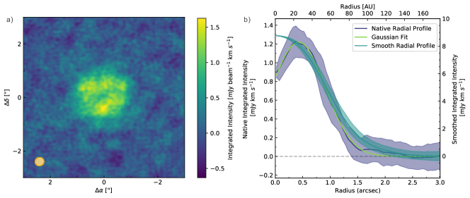
Figure 3: Left panel: Integrated intensity map made from the stacked 6 transitions. The noise is calculated to be 0.14 mJy beam^-1km s^-1. Right panel: the azimuthally averaged integrated intensity radial profile obtained from the stacked native resolution data. Shaded areas represent $1\sigma$ uncertainties, where $\sigma$ represents the standard deviation in each radial bin.

3 CH2CN Excitation Analysis

The rotational temperature, $T_{\rm rot}$, and the total column density of CH2CN, N, can be constrained through the use of a rotational diagram analysis. This implicitly assumes that the molecular excitation can be described by a single temperature and that the molecules are in local thermodynamic equilibrium (LTE). As we assume that the critical densities for CH2CN and CH3CN are similar ($2.0\times 10^{6}$ cm^-3 and $2.6\times 10^{6}$ cm^-3 for the transitions $J=13-12$ and $J=12-11$ at 40 K, respectively), and that chemical models of TW Hya suggest that even atmospheric densities exceed $10^{9}$ cm^-3 (e.g., Cleeves et al., 2015), it is reasonable to assume that both CH2CN would be thermalized. As such, we can assume that the excitation temperature is equal to the gas kinetic temperature (Shirley, 2015; Guzmán et al., 2018; Loomis et al., 2018a). These parameters allow us to draw conclusions about the physical conditions where CH2CN is found and its potential interactions with molecules that exist in a similar environment.

3.1 Method

We start our analysis by constraining the disk-averaged rotational temperature, $T_{\rm rot}$, and the total column density, $N$. Following Goldsmith & Langer (1999), we obtain the rotational diagram shown in Figure 4A by using the equation

$$\ln\frac{{N_{\rm{u}}^{\rm thin}}}{g_{\rm u}}+\ln C_{\tau}=\ln N-\ln Q(T_{\rm rot})-\frac{E_{\rm u}}{kT_{\rm rot}},$$ (2)

where $N_{\rm{u}}^{\rm thin}$ is the column density of molecules in the upper state of each transition without the correction for the optical depth effect, $C_{\tau}$ is the optical correction factor, and $Q(T_{\rm rot})$ is the molecular partition function and $E_{\rm u}$ is the upper state energy. We use the molecular partition function from The Cologne Database for Molecular Spectroscopy (CDMS; Müller et al., 2001) using a linear interpolation to obtain our $Q$ values (Endres et al., 2016). Degeneracies due to the hyperfine structure are included in the calculation of $Q$.

We calculate the $N_{\rm{u}}^{\rm thin}$ for each transition through the equation:

$$N_{\rm{u}}^{\rm thin}=\frac{4\pi S_{v}\Delta v}{A_{\rm ul}\Omega hc},$$ (3)

where $A_{\rm ul}$ is the Einstein coefficient, $S_{\nu}$ is the disk-averaged integrated flux density calculated as described in §2.2 and using a bin-size of 2.5″, $\Delta$ is the width of the two channels that we used for integration and $\Omega$ is the solid angle subtended by the source.

The optical correction factor is obtained through the equation:

$$C_{\tau}=\frac{\tau}{1-e^{-\tau}}.$$ (4)

where the optical depth, $\tau$, can be related to the upper level population through the equation:

$$\tau_{\rm ul}=\frac{A_{\rm ul}c^{3}}{8\pi\nu^{3}\Delta v}N_{u}(e^{h\nu/kT_{\rm rot}}-1).$$ (5)

Given that our emission is dominated by Doppler broadening, the line width, $\Delta v$, is given by

$$\Delta v=\sqrt{\frac{2kT_{\rm rot}}{m_{u}\,m_{H}}},$$ (6)

with $m_{u}$ being the molecular weight of CH₂CN (40 g/mol) and $m_{H}$ being the mass of a hydrogen atom.

We create a model that relates $N_{u}$, $C_{\tau}$ and $\Delta v$ to Equation 2 and we derive the values of $T_{\rm rot}$ and $N$ by matching the observed $N_{u}/g_{u}$ values. We use Scipy’s curve_fit function to minimize $\chi^{2}$ and find the best estimate of our desired parameters (Jones et al., 2001). $\ln(N_{u}/g_{u})$ can then be plotted against the upper state energies, $E_{u}$ to obtain Figure 4A, where the slope and the $y$-intercept of the line respectively represent $-T_{\rm rot}^{-1}$ and $N$.

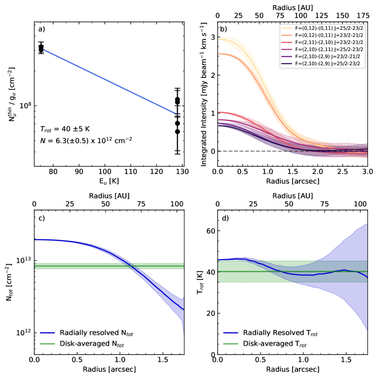
Figure 4: Panel A: ortho-CH2CN disk-averaged rotational diagram. Panel B: the radial profiles for the six detected transitions. Shaded areas represent 1$\sigma$ uncertainties. Panels C & D: radial profiles of respectively the CH2CN total column density and the rotational temperature. The colour dark blue indicates radially resolved values, whereas green is used for values we obtained from disk-averaged analysis. Shaded areas represent 1$\sigma$ uncertainties.

3.2 Disk-averaged Analysis

Table 2: Formation and destruction pathways for CH2CN

Reaction	Reactants			Products		Mechanism	Rates of Reaction
Type							$\alpha$ $[{\rm cm^{3}~{}s^{-1}}]$	$\beta$	$\gamma$	rate type
Formation	CN	CH3	->	H	CH2CN	Neutral-Neutral	$1.00(-10)$	$0.00$	0.00	(1)
	N	C2H3	->	H	CH2CN	Neutral-Neutral	$6.40(-11)$	$0.17$	$0.00$	(1)
	C	CH2NH	->	H	CH2CN	Neutral-Neutral	$1.00(-10)$	$0.00$	$0.00$	(1)
	CH3CN+	$e^{-}$	->	H	CH2CN	DR	$2.00(-7)$	$-0.50$	$0.00$	(1)
	CH3CNH+	$e^{-}$	->	2H	CH2CN	DR	$8.00(-8)$	$-0.50$	$0.00$	(1)
	s-CN	s-CH2	->	CH2CN		Grain Surface
Destruction	CH2CN	C+	->	C	CH2CN+	Ion-Polar	$1.00$	$1.61(-9)$	$5.81$	(2)
	CH2CN	H${}_{3}^{+}$	->	H2	CH3CN+	Ion-Polar	$1.00$	$2.94(-9)$	$5.81$	(2)
	CH2CN	h$\nu{}$	->	CN	CH2	Photodissociation	$1.56(-9)$	$0.00$	$1.95$	(3)
	CH2CN	h$\nu{}$	->	CH2CN+	e-	Photodissociation	$5.29(-10)$	$0.00$	$3.11$	(3)
	CH2CN		->	s-CH2CN		Freeze-out

Note. — Table showing all the possible formation and destruction pathways of CH2CN based on the astrochemical disk model by Le Gal et al. (2019). The rates of reactions are reproduced from the Kinetic Database for Astrochemistry available at http://kida.astrophy.u-bordeaux.fr (Wakelam et al., 2012).

In this paper, we will denote the column density of ortho-CH2CN using N, whereas the total column density of CH2CN (including both the ortho and the para isomers) will be indicated using $N_{\rm tot}$. We obtain a disk-averaged rotational temperature of $40\pm 5$ K and a disk-averaged total column density, $N$, of $(6.3\pm 0.5)\times 10^{12}$ cm^-2 for ortho-CH2CN. As described in Le Gal et al. (2017), for a molecule containing two identical Hydrogen nuclei, such as CH2CN, we expect a statistical ortho/para ratio of 3:1, and therefore we infer a total column density, $N_{\rm tot}$, of $(8.4\pm 0.7)\times 10^{12}$ cm^-2. Indeed, due to the $X^{2}$B1 symmetry of the ground electronic state of CH2CN, the ortho-to-para ratio of CH2CN decreases toward the statistical 3:1 value with increasing temperature as NH2 (Le Gal et al., 2016). CH2CN is a heavier molecule than NH2, therefore, its ortho-to-para ratio will reach the statistical ratio for lower temperatures than NH2. Thus, according to Fig. 1 of Le Gal et al. (2016), the relatively high rotational temperature we derived confirms that it is reasonable to consider a 3:1 statistical ortho-para ratio for CH2CN. Given this ratio, we can calculate the expected para column density and using this value and the the expected integrated intensity of the para lines that we do not detect (located at 241.353 and 241.381).

Finally, having obtained $T_{\rm rot}$, we calculate the optical depth, $\tau$, of our transitions. In all cases, we obtained a value of $\tau\ll 1$, with values of range $4\times 10^{-4}$ to $3.4\times 10^{-3}$. Therefore, our detected transitions were of negligible optical thickness. In addition to this, using these parameters we can calculate the predicted strength of the lines that we do not detect. For the transitions at 241.353 and at 241.382 (which belong to para-CH2CN) we obtain integrated intensities of 1.26 and 1.37 mJy km s-1, which are significantly below our calculated intensities, thus confirming that we would not have been able to detect these lines with our spectral set-up. The disk-averaged values obtained in Section 3.1 are calculated out to a radius of 1.75″ as we can see from Figure 4b that at this radius, all six transitions are detected. As a comparison, we calculate an average $T_{\rm rot}$ and $N$ for the outer region of the disk where the weaker emission lines are almost completely lost. For this, we integrated out to a radius of 2.5″. For this outer region, we find a total column density of $(3.5\pm 0.3)\times 10^{12}$ ($(4.7\pm 0.4)\times 10^{12}$ for ortho-CH2CN) cm^-2, and a rotational temperature of $38\pm 5$ K. Comparing the total column density that we obtained out to a radius 1.75″ to that out to 2.5″ confirms that the outer radii are contributing very little to the total column density, as we would expect from the radial profiles in Figure 4B and in the right panel of Figure 3.

3.3 Radially Resolved Analysis

To further observe the behaviour of $T_{\rm rot}$ and N_tot across the disk, we use the radial integrated intensities from each of the transitions in Figure 4B and we repeat the steps outlined in Section 3.2 to obtain rotational diagrams at different radii. The results are summarised in panel 4C and D.

Figure 4C shows that the column density decreases from $5\times 10^{13}$ to $0.6\times 10^{13}$ cm^-2across the radius of the disk. This is consistent with the disk-averaged column density. The $T_{\rm rot}$ ranges between 45 and 37 K, which is consistent with the disk-averaged $T_{\rm rot}$ (40 $\pm$5 K). We note that this is very similar to the CH3CN excitation temperature of $32.7^{+3.9}_{-3.4}$ K in the same disk (Loomis et al., 2018a). On the other hand, the column density of CH3CN, $1.82^{+0.25}_{-0.19}\times 10^{12}$ cm^-2, is $\sim$10 times lower than our observed CH2CN’s $N_{\rm tot}$. This is consistent with our chemical model, as discussed in Section 4.1.

4 Discussion

4.1 CH2CN/CH3CN Ratio & Disk Models Results

We use the chemical models by Le Gal et al. (2019) to explore the predicted column densities of CH2CN and CH3CN as a function of radius, as shown in Figure 5a & b. The original model has been modified to fit TW Hya using the physical parameters described in Table 3, and a standard cosmic-ray ionization rate of $1\times 10^{-17}$ s^-1. We used a C/O ratio of 1 which was the best C/O ratio found in Le Gal et al. (2019) to reproduce the column densities of the nitriles detected in abundance in disks. Overall, the model is in good accordance with our observations as it predicts that CH2CN is more abundant than CH3CN at all radii. However, the CH2CN/CH3CN ratio in the model is larger than the ratio of $\sim$5 we found observationally. Inspecting Fig. 5a&b, we see that the model correctly predicts the column density of CH2CN and under-predicts that of CH3CN. This suggests that while the column density of CH2CN is well reproduced by standard astrochemical model assumptions, there are missing chemical pathways that lead to the formation of CH3CN. Detailed astrochemical disk modeling effort needs to be made to further constrain the main reaction pathways driving both the observed CH3CN abundance and CH2CN/CH3CN ratio in the TW Hya protoplanetary disk, but they are beyond the scope of this paper and will be the subject of a future dedicated study. For now, the use of chemical models allows us to confirm that a ratio of CH2CN/CH3CN$>$1 is indeed plausible in our disk and allows us to give a more comprehensive overview of CH2CN in TW Hya. Figure 5c&d show the abundance distribution of CH3CN and CH2CN with respect to height and the radius of TW Hya. Once again, we can see that CH2CN is more abundant than CH3CN at all radii and heights in the disk and that the region of brightest emission for both of these molecules is co-localised and between a radius of $\sim$50-100 au and a height of $\sim$10 au. This is consistent with our observations as the model in Figure 5a shows that our observed $N_{\rm tot}$ for CH2CN arises from a radius of $\sim$100 au.

Table 3: Physical parameters used for the disk chemistry modeling

Parameters	TW Hyaa
Stellar mass: $M_{\star}$ ($M_{\odot}$)	0.8
Characteristic radius: $R_{\rm{c}}$ (AU)	10
Density power-law index	1.5
Midplane temperature at $R_{\rm{c}}$ (K)	20
Atmosphere temperature at $R_{\rm{c}}$ (K)	104
Surface density at $R_{\rm{c}}$ (g cm-2)	0.79
Temperature power-law index	0.55
Vertical temperature gradient index	2
UV Fluxb at $R_{\rm{c}}$ (in Draine (1978b)’s units)	3400

• ^a Andrews et al. (2012)

• ^b Herczeg et al. (2004)

4.2 CH2CN Chemistry

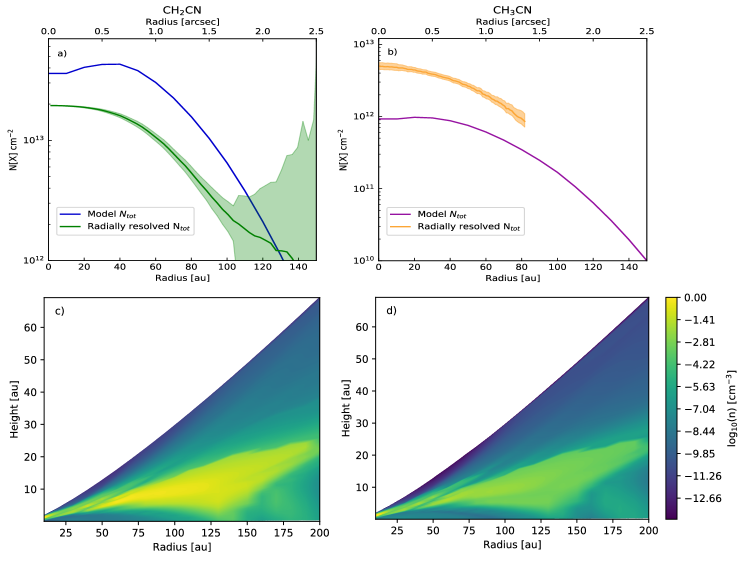
Figure 5: Panel a) & b): Total column densities of CH2CN (a) and CH3CN (b) as a function of radius, predicted by the chemical models of Le Gal et al. (2019) that we adapted to TW Hya as described in §4.1. The column density radial profile derived from the observations presented in Sect. 3.3 for CH2CN (a) from the observation of CH3CN obtained by Loomis et al. (2018a) (b) are also shown. Panel c) & d): The abundance of CH2CN and CH3CN as a function of radius and height. The region of highest emission for both molecules is located between $\sim 50-100$ au and at a height of $\sim 10$ au.

Formation of molecular species in protoplanetary disks can occur via two distinct routes: gas-phase and grain-surface reactions, and in the case of CH2CN both pathways are a priori possible. Based on the astrochemical disk model of Le Gal et al. (2019), several formation and destruction pathways are involved in the chemistry of CH2CN. These are summarized in Table 2.

As previously mentioned, CH3CN and CH2CN are found to have similar excitation temperatures and morphologies, therefore it is unsurprising that they also share a comparable chemistry. Both CH3CN and CH2CN share a very similar grain-surface formation chemistry where both can be formed via solid state reactions with CN as follows,

(7)

(Herbst, 1985). From these reactions we can infer that the relative formation rates of CH3CN and CH2CN will depend on the relative abundance of CH2 and CH3 radicals on the grain surface. The similarities extend beyond these grain-surface reactions, as these molecules share a common gas-phase reaction pathway. The electronic dissociative recombination of CH3CNH+ has been identified as the dominant contributor to the gas-phase formation of both CH3CN and CH2CN (Vastel et al., 2015; Loomis et al., 2018a). The full reaction route, including the formation of the ion intermediate, is as follows:

(8)

(9)

(Herbst & Leung, 1990). This does not seem to be the main formation pathway for CH2CN in either the model or in ‘reality’ since the electronic dissociative recombination (DR) of CH3CNH+ leads to a branching ratio of $\sim$1.5 in favour of CH3CN according to the Kinetic Database for Astrochemistry (see Table 2) while we find that CH2CN $\gg$ CH3CN. The branching ratio for this reaction is arbitrary and it is loosely based on the fact that the energy in the CH3CN + H channel is greater than the secondary dissociation energy in the CH2CN + 2H channel (Wakelam et al., 2012). In light of this, we suggest that the grain surface formation pathway is the most important source of CH2CN in disks. A similar conclusion was made with respect to CH3CN by (Le Gal et al., 2019) and (Loomis et al., 2018a). However, grain-surface reactions are poorly constrained both theoretically and experimentally and therefore more experimental studies need to be carried out to verify the significance of this solid-state reaction. Finally we note that CH2CN can also form through several neutral-neutral reactions (Table 2), whose possible contributions also warrant further investigation.

4.3 Morphology

As mentioned in Section 2.2, CH2CN is found in a ring morphology when imaged at the native resolution of $\approx 0.3\arcsec{}$. The ring morphology is not unique to CH2CN as CN and C2H are also analogously distributed in TW Hya, however, their rings peak at considerably larger radii at $\sim$ 45 au (0.75″) and 60 au (1″), respectively (Bergin et al., 2016; Teague & Loomis, 2020). These nested rings of potentially chemically related species provide clues as to what processes are regulating the abundance of these molecules. One possible source of rings is the increased penetration of UV radiation beyond the edge of the dust continuum, leading to more photo-desorption of frozen out molecules from grain surfaces (Cleeves, 2016). However, the edge of the dust continuum is at $\sim 60$ au, which is inconsistent with the peak of the CH2CN ring ($\sim 24$ au) therefore this is not a plausible explanation for the morphology of CH2CN.

The chemical model results for CH2CN shown in Figure 5 seem to replicate the morphology that we observed in Figure 4C. This suggests the presence of a ‘Goldilocks zone’ for the dominant formation pathway where the observed morphology can be attributed to the balance between formation and destruction reactions under fiducial disk conditions. Within this zone of the disk, the conditions may be particularly favourable for the production of CH2CN (i.e. optimal UV radiation flux or temperature of the disk molecular layer).

Another possible factor that could shape the distribution of CH2CN is enhanced destruction in the inner disk due to reactions with gas-phase carbon and oxygen atoms. Chemical modeling by Du et al. (2015) has shown that C and O depletion is needed to reproduce the observed molecular abundances of CO and H2O in TW Hya. Further, nitrile column density is enhanced by $\sim$2 orders of magnitude where C and O depletion takes place (Du et al., 2015). One disk location that may present a rapid change in the C and O abundance is the CO snowline, where CO ice sublimates back into the gas-phase. The CO snowline zone in TW Hya is found at 17-30 au (Schwarz et al., 2016; Qi et al., 2013). We find that CH2CN peaks at $\sim$ 24 au, so the CO snowline and the CH2CN peak may reflect the presence of C- and O-depleted gas just exterior to the CO snowline. Exterior to this region, carbon and oxygen would primarily exist as CO ice, therefore not interfere with nitrile chemistry.

5 Summary

We have presented the first detection of CH2CN (cyanomethyl) in a protoplanetary disk. The 6 emission lines detected correspond to 6 transitions of CH2CN in its ortho state. We find a disk-averaged rotational temperature of $40\pm 5$ K and a disk-averaged total column density of $(6.3\pm 0.5\times 10^{12}$ cm^-2. Assuming a thermal ortho/para ratio of 3:1, we infer a total CH2CN column density of $(8.4\pm 0.7)\times 10^{12}$ cm^-2. The molecule is observed to be in a ring whereas at lower spatial resolutions it presents a centrally-peaked profile consistent with previously reported CH3CN morphology. Comparison with CH3CN total column density shows that CH2CN is 10 times more abundant. This result is consistent with chemical models for TW Hya, where CH2CN$\gg$CH3CN at all disk radii. We identify possible pathways that contribute to the formation and destruction of this molecule and we suggest that grain-surface reactions are the likely formation pathway for both CH2CN and CH3CN.

References

- Agúndez et al. (2008) Agúndez, M., Fonfría, J. P., Cernicharo, J., Pardo, J. R., & Guélin, M. 2008, A&A, 479, 493, doi: 10.1051/0004-6361:20078956
- Altwegg et al. (2020) Altwegg, K., Balsiger, H., Hänni, N., et al. 2020, Nature Astronomy, 4, 533, doi: 10.1038/s41550-019-0991-9
- Andrews et al. (2012) Andrews, S. M., Wilner, D. J., Hughes, A. M., et al. 2012, ApJ, 744, 162, doi: 10.1088/0004-637X/744/2/162
- Andrews et al. (2018) Andrews, S. M., Huang, J., Pérez, L. M., et al. 2018, ApJ, 869, L41, doi: 10.3847/2041-8213/aaf741
- Bailer-Jones et al. (2018) Bailer-Jones, C. A. L., Rybizki, J., Fouesneau, M., Mantelet, G., & Andrae, R. 2018, AJ, 156, 58, doi: 10.3847/1538-3881/aacb21
- Bergin et al. (2016) Bergin, E. A., Du, F., Cleeves, L. I., et al. 2016, ApJ, 831, 101, doi: 10.3847/0004-637X/831/1/101
- Bergner et al. (2018) Bergner, J. B., Guzmán, V. G., Öberg, K. I., Loomis, R. A., & Pegues, J. 2018, ApJ, 857, 69, doi: 10.3847/1538-4357/aab664
- Chapillon et al. (2012) Chapillon, E., Dutrey, A., Guilloteau, S., et al. 2012, ApJ, 756, 58, doi: 10.1088/0004-637X/756/1/58
- Cleeves (2016) Cleeves, L. I. 2016, ApJ, 816, L21, doi: 10.3847/2041-8205/816/2/L21
- Cleeves et al. (2015) Cleeves, L. I., Bergin, E. A., Qi, C., Adams, F. C., & Öberg, K. I. 2015, ApJ, 799, 204, doi: 10.1088/0004-637X/799/2/204
- Draine (1978a) Draine, B. T. 1978a, ApJS, 36, 595, doi: 10.1086/190513
- Draine (1978b) —. 1978b, ApJS, 36, 595, doi: 10.1086/190513
- Du et al. (2015) Du, F., Bergin, E. A., & Hogerheijde, M. R. 2015, ApJ, 807, L32, doi: 10.1088/2041-8205/807/2/L32
- Dutrey et al. (1997) Dutrey, A., Guilloteau, S., & Guelin, M. 1997, A&A, 317, L55
- Endres et al. (2016) Endres, C. P., Schlemmer, S., Schilke, P., Stutzki, J., & Müller, H. S. P. 2016, Journal of Molecular Spectroscopy, 327, 95, doi: 10.1016/j.jms.2016.03.005
- Goldsmith & Langer (1999) Goldsmith, P. F., & Langer, W. D. 1999, ApJ, 517, 209, doi: 10.1086/307195
- Guzmán et al. (2018) Guzmán, V. V., Öberg, K. I., Carpenter, J., et al. 2018, ApJ, 864, 170, doi: 10.3847/1538-4357/aad778
- Guzmán et al. (2015) Guzmán, V. V., Öberg, K. I., Loomis, R., & Qi, C. 2015, ApJ, 814, 53, doi: 10.1088/0004-637X/814/1/53
- Herbst (1985) Herbst, E. 1985, ApJ, 291, 226, doi: 10.1086/163060
- Herbst & Leung (1990) Herbst, E., & Leung, C. M. 1990, A&A, 233, 177
- Herczeg et al. (2004) Herczeg, G. J., Wood, B. E., Linsky, J. L., Valenti, J. A., & Johns-Krull, C. M. 2004, ApJ, 607, 369, doi: 10.1086/383340
- Hily-Blant et al. (2017) Hily-Blant, P., Magalhaes, V., Kastner, J., et al. 2017, A&A, 603, L6, doi: 10.1051/0004-6361/201730524
- Huang et al. (2018) Huang, J., Andrews, S. M., Cleeves, L. I., et al. 2018, ApJ, 852, 122, doi: 10.3847/1538-4357/aaa1e7
- Irvine et al. (1988) Irvine, W. M., Friberg, P., Hjalmarson, A., et al. 1988, ApJ, 334, L107, doi: 10.1086/185323
- Jones et al. (2001) Jones, E., Oliphant, T., & Peterson, P. 2001
- Kastner et al. (1997) Kastner, J. H., Zuckerman, B., Weintraub, D. A., & Forveille, T. 1997, Science, 277, 67, doi: 10.1126/science.277.5322.67
- Le Gal et al. (2019) Le Gal, R., Brady, M. T., Öberg, K. I., Roueff, E., & Le Petit, F. 2019, ApJ, 886, 86, doi: 10.3847/1538-4357/ab4ad9
- Le Gal et al. (2016) Le Gal, R., Herbst, E., Xie, C., Li, A., & Guo, H. 2016, A&A, 596, A35, doi: 10.1051/0004-6361/201629107
- Le Gal et al. (2017) Le Gal, R., Xie, C., Herbst, E., et al. 2017, A&A, 608, A96, doi: 10.1051/0004-6361/201731566
- Liszt et al. (2018) Liszt, H., Gerin, M., Beasley, A., & Pety, J. 2018, ApJ, 856, 151, doi: 10.3847/1538-4357/aab208
- Loomis et al. (2018a) Loomis, R. A., Cleeves, L. I., Öberg, K. I., et al. 2018a, ApJ, 859, 131, doi: 10.3847/1538-4357/aac169
- Loomis et al. (2018b) Loomis, R. A., Öberg, K. I., Andrews, S. M., et al. 2018b, AJ, 155, 182, doi: 10.3847/1538-3881/aab604
- McGuire (2018) McGuire, B. A. 2018, ApJS, 239, 17, doi: 10.3847/1538-4365/aae5d2
- McMullin et al. (2007) McMullin, J. P., Waters, B., Schiebel, D., Young, W., & Golap, K. 2007, in Astronomical Society of the Pacific Conference Series, Vol. 376, Astronomical Data Analysis Software and Systems XVI, ed. R. A. Shaw, F. Hill, & D. J. Bell, 127
- Müller et al. (2001) Müller, H. S. P., Thorwirth, S., Roth, D. A., & Winnewisser, G. 2001, A&A, 370, L49, doi: 10.1051/0004-6361:20010367
- Mumma & Charnley (2011) Mumma, M. J., & Charnley, S. B. 2011, ARA&A, 49, 471, doi: 10.1146/annurev-astro-081309-130811
- Nomura et al. (2016) Nomura, H., Tsukagoshi, T., Kawabe, R., et al. 2016, ApJ, 819, L7, doi: 10.3847/2041-8205/819/1/L7
- Oberg (2016) Oberg, K. I. 2016, arXiv e-prints, arXiv:1609.03112. https://arxiv.org/abs/1609.03112
- Oberg & Bergin (2020) Oberg, K. I., & Bergin, E. A. 2020, arXiv e-prints, arXiv:2010.03529. https://arxiv.org/abs/2010.03529
- Öberg et al. (2015) Öberg, K. I., Guzmán, V. V., Furuya, K., et al. 2015, Nature, 520, 198, doi: 10.1038/nature14276
- Patel et al. (2015) Patel, B. H., Percivalle, C., Ritson, D. J., Duffy, C. D., & Sutherland, J. D. 2015, Nature Chemistry, 7, 301, doi: 10.1038/nchem.2202
- Powner et al. (2009) Powner, M. W., Gerland, B., & Sutherland , J. D. 2009, Nature, 459, 239, doi: 10.1038/nature08013
- Qi et al. (2003) Qi, C., Kessler, J. E., Koerner, D. W., Sargent, A. I., & Blake, G. A. 2003, ApJ, 597, 986, doi: 10.1086/378494
- Qi et al. (2013) Qi, C., Öberg, K. I., Wilner, D. J., et al. 2013, Science, 341, 630, doi: 10.1126/science.1239560
- Schwarz et al. (2016) Schwarz, K. R., Bergin, E. A., Cleeves, L. I., et al. 2016, ApJ, 823, 91, doi: 10.3847/0004-637X/823/2/91
- Shirley (2015) Shirley, Y. L. 2015, PASP, 127, 299, doi: 10.1086/680342
- Teague (2019a) Teague, R. 2019a, The Journal of Open Source Software, 4, 1632, doi: 10.21105/joss.01632
- Teague (2019b) —. 2019b, Research Notes of the AAS, 3, 74, doi: 10.3847/2515-5172/ab2125
- Teague & Loomis (2020) Teague, R., & Loomis, R. 2020, ApJ, 899, 157, doi: 10.3847/1538-4357/aba956
- van Dishoeck (1994) van Dishoeck, E. F. 1994, in Astronomical Society of the Pacific Conference Series, Vol. 58, The First Symposium on the Infrared Cirrus and Diffuse Interstellar Clouds, ed. R. M. Cutri & W. B. Latter, 319
- Vastel et al. (2015) Vastel, C., Yamamoto, S., Lefloch, B., & Bachiller, R. 2015, A&A, 582, L3, doi: 10.1051/0004-6361/201527153
- Wakelam et al. (2012) Wakelam, V., Herbst, E., Loison, J. C., et al. 2012, ApJS, 199, 21, doi: 10.1088/0067-0049/199/1/21
- Walsh et al. (2016) Walsh, C., Loomis, R. A., Öberg, K. I., et al. 2016, ApJ, 823, L10, doi: 10.3847/2041-8205/823/1/L10
- Woon & Herbst (2009) Woon, D. E., & Herbst, E. 2009, ApJS, 185, 273, doi: 10.1088/0067-0049/185/2/273