Architecture and Performance Evaluation of Distributed Computation Offloading in Edge Computing

Abstract

Edge computing has been proposed to cope with the challenging requirements of future applications, like mobile augmented reality, since it shortens significantly the distance, hence the latency, between the end users and the processing servers. On the other hand, serverless computing is emerging among cloud technologies to respond to the need of highly scalable event-driven execution of stateless tasks. In this paper, we first investigate the convergence of the two to enable very low-latency execution of short-lived stateless tasks, whose computation is offloaded from the user terminal to servers hosted by or close to edge devices. We tackle in particular the research challenge of selecting the best executor, based on real-time measurements and simple, yet effective, prediction algorithms. Second, we propose a performance evaluation framework specifically designed for an accurate assessment of algorithms and protocols in edge computing environments, where the nodes may have very heterogeneous networking and processing capabilities. The proposed framework relies on the use of real components on lightweight virtualization mixed with simulated computation and is well-suited to the analysis of several applications and network environments. Using our framework, we evaluate our proposed architecture and algorithms in small- and large-scale edge computing scenarios, showing that our solution achieves similar or better delay performance than a centralized solution, with far less network utilization.

1 Introduction

Edge computing is generally considered the principal enabling technology for several applications with stringent latency requirements [1]. With edge computing the functions that were located in a remote data center in a Mobile Cloud Computing (MCC) architecture are called back to some point nearer to the user [2], e.g., networking devices in the access network with spare or added computational capabilities. Edge computing technologies are being driven by vertical market segments, including: Internet of Things (IoT), for which a reference architecture has been published by the OpenFog Consortium [3]; the automotive and mobile network domains, which are of great interest to the telecom industry, which has recently standardized an inter-operable Multi-access Edge Computing (MEC) within European Telecommunications Standards Institute (ETSI) [4]. However, edge computing has its limitations when used in a pervasive environment with mobile devices: as shown in Fig. 1 (a) once an application has been provisioned on a given edge node, which is optimal for the current user position, if the user roams towards a different point of attachment the network must either accept increased latency due to sub-optimal routing (top part) or pay the cost of a migration of the application to another edge node (bottom part), which could also cause a service interruption.

In this paper we provide two major contributions. Firstly, we propose to overcome the above limitation by adopting a serverless computing approach. Secondly, we recognize that the tools for the performance evaluation of edge computing systems are quite limited, notwithstanding the high interest in this technology, hence we propose a novel framework for the performance analysis that is suitable to a wide range of conditions of practical interest. Both contributions are introduced briefly in the following.

Serverless computing [5] is a novel paradigm originating from cloud computing where clients request the execution of short-lived “light” jobs, e.g, a script in a given run-time environment, most often Python or Node.js. Such jobs are stateless, hence they do not require a full life-cycle management of the application nor the persistent allocation of resources on the remote server. This way, inherent scalability is achieved: ideally, no performance bottleneck exists as the number of clients grows, as long as new locations for the execution of tasks are added. Amazon has been among the first to offer a commercial service for serverless computing, called AWS Lambda, closely followed by Microsoft Azure functions and Google Cloud functions. Existing solutions for serverless computing, such as Apache OpenWhisk and Knative, adopt a logically centralized load balancer to dispatch the jobs to the servers, as show in Fig. 1 (b). However, such serverless computing platforms cannot be used for computation offloading of delay-sensitive pervasive applications in edge networks, because in this context both the clients and the edge servers are distributed in a large geographical area and are interconnected with links having limited capacity and introducing significant delays, compared to the maximum tolerable latency.

Figure 1: Comparison of architectures for (a) edge computing, (b) serverless computing, and (c) proposed merge of the two.

Therefore, we propose a solution for the execution of stateless jobs, called lambda functions, on edge nodes as illustrated in Fig. 1 (c) where we have: computers, which have computational capabilities to offer, because either they have spare resources, as often found in many networking devices, or they have been provisioned specifically for this purpose; clients, which are User Terminals wishing to use said capabilities because it is impossible or inefficient for them to perform the computation directly; dispatchers, which are the entry points to the edge computing domain for clients. Clients perform Remote Procedure Calls on the dispatchers, which select the most suitable computer to run each function, forward to it the client request, then get back the result to the client. The RPC is short-lived: the input is contained in the request, the output in the response, and the call is closed immediately after completion to avoid the persistence of long-term states in the network. The architecture is fully distributed: dispatchers use only their local information to take decisions on which computer should execute the incoming function. Because of the ephemeral nature of lambda transactions, these decisions are not affected by the relocation of Virtual Machine (VM)/containers on computers, which happens far more sporadically. The proposed architecture is a step forward compared to existing alternatives, reviewed in Sec. 2.1. In particular, as described in Sec. 3.1, it achieves: (i) low latency, since we cut away all the detours through the centralized decision point; (ii) scalability, because the size of the decision problem at each dispatcher grows linearly with the number of computers; (iii) reliability, as the failure of a dispatcher only affects the clients currently using it while the rest of the system runs without degradation. Among the many research challenges associated to the proposed architecture, in this paper we focus specifically on the online dispatch algorithm to select the computer that will run a given function at a given time, which is tackled in Sec. 3.2. As discussed in further details in Sec. 2.2, state of the art solutions address on the one hand edge scenarios where tasks last much longer than in our case, and therefore tasks allocations need to be decided and changed much less frequently than in our reference environment. On the other hand, when tasks are “light-weight” as in our case, the target scenario is typically that of tasks scheduling in multi-core data centers, which is clearly a much more controlled and centralized environment than ours.

With regard to the performance evaluation of edge computing, in Sec. 2.3 we review the existing approaches, which we have classified into four categories: mathematical models; cloud models; packet-level simulations; testbed experiments. We show that all these approaches are very well suited to capture only a portion of the complexity incurred by an edge computing system, where the nodes may have heterogeneous capabilities and connectivity, and the Key Performance Indicators are affected by both computation and communication aspects, which are hard to capture at the same time. In Sec. 4 we propose a novel framework for the evaluation of algorithms and protocols in an edge computing environment, which surpasses the limitations of the existing alternatives. We argue that this framework, which relies on network emulation, application-based virtualization, and (partial) simulation of computation elements, is general enough to support a wide range of environments. To validate the framework and, at the same time, show the effectiveness of our proposed online dispatching algorithm, we implemented the key components of serverless edge computing and performed an extensive campaign of experiments, whose results are reported in Sec. 5. The online dispatch algorithm has been compared with a centralized approach, as commonly found in serverless computing in data centers, and a known online algorithm from the literature [6].

2 State of the art

In this section we review the state of the art in the literature, separately for the main contributions of this work: architecture for the convergence of the edge computing and serverless computing paradigms (Sec. 2.1); distributed dispatching of lambda functions to computers (Sec. 2.2); modeling and large-scale simulation of edge computing environments (Sec. 2.3).

2.1 Converged serverless edge computing architecture

In the scientific literature there are several proposals on how to realize computation offloading in edge computing. However, the vast majority are based on some form of lightweight orchestration, as compared to having a true “cloud” with VMs, by scaling down cloud-oriented paradigms to less powerful servers and faster dynamics. Examples include Picasso [7], from which we reuse the concept of providing the applications with an Application Programming Interface (API) whose routines are executed by the network in a manner transparent to clients, and foglets [8], which use containers for an easier and faster migration of functions based on situation-awareness schemes. Both studies put forward efficient ways to periodically tune the deployment of containers in edge servers, which is complementary to our work, where we focus instead on the short time scale dispatching of tasks once a given deployment in place.

In addition to generic architectures, such as what we propose in this paper, there are solutions tailored to specific scenarios. In [9] the authors exploit Information-Centric Networking (ICN) to realize a paradigm called Named Function as a Service (NFaaS), where the functions are automatically distributed over ICN-enabled servers based on their utilization. Again, this could be a suitable complement to our present contribution, where we focus mostly on the short-term dispatch problem over an interval small enough that we can assume that the functions on the computers are stable. It is interesting to point out that to reduce the latency of setting up/tearing down the application, it is suggested that the servers employ unikernels [10], which are an extreme form of containerization. In the context of IoT, a cloud-edge architecture is proposed in [11], which employs micro-services to run computation on heterogeneous edge or cloud nodes: different algorithms are proposed to schedule tasks from the clients, in the assumption that a centralized scheduling engine can estimate at fine grain both the task processing time and the time it will be put into service, which is advocated to be realistic in some conditions, i.e., with a priori knowledge on the application algorithms and continuous monitoring of the computation engines. When applying the constraints of our use case to the scheduling policies considered there, they basically collapse into scheduling every task to the computer with shortest expected processing time, which is exactly what we propose in Sec. 3.2. Finally, also in the context of IoT in [12] the authors propose an architecture to distribute jobs to a set of gateways by means of dynamic data plane manipulation: since all the client requests pass through the Software Defined Networking (SDN) controller, the latter can estimate the arrival process and allocate new requests to servers accordingly. Unfortunately, such information is not available in a fully distributed approach such as ours.

2.2 Distributed dispatching of lambda functions

From a high level perspective, the distributed dispatching problem can be described as follows, from the point of view of a given dispatcher. There are a number of lambda functions (or jobs) that will arrive over time and will have to be dispatched to a pool of computers, with the goal of minimizing their response time. The arrival process and the execution times are not known a priori. So far, this is a set-up for a classical multi-server scheduling problem, that has been extensively studied in the literature due to its huge importance in designing efficient schedulers in multi-core systems, both stand-alone and in grid/cloud environments. A known result is that no online algorithm can have a bounded competitive ratio, see, e.g., [13]. In the same work the authors also propose a method to derive approximation algorithms that have a bounded competitive ratio in a speed augmentation model, i.e., by assuming that the online algorithm is given extra resources. One major difference with an edge computing scenario is that the multi-server scheduling problem assumes that the servers are used exclusively and that the policy for the execution of the jobs within each server is also under control. Both assumptions are false in our system: (i) any computer can be assigned jobs by multiple non-communicating dispatchers, and (ii) we cannot reasonably assume to have influence (or even insight!) on the scheduling within computers, which are highly heterogeneous (ranging from a Wireless Local Area Network (WLAN) routers to multi-core servers in a Mobile Network Operator (MNO) core network) and shared (e.g., a telco server may offer computational capabilities while also implementing Virtual Network Functions). Furthermore, different computers may have different communication latencies with the dispatcher, and they may vary over time since the network of an edge computing domain is expected to be also (well, actually mostly) used for Internet access.

A closer view is taken in [6], which in fact deals more specifically with edge computing. The authors propose an approximation algorithm to minimize the total weighted latency of the jobs, where the weight is assumed to be generically related to the delay-sensitiveness of the job. The algorithm is proved to be $\mathcal{O}(1/\epsilon)$-competitive in the $(1+\epsilon)$-augmented problem. The algorithm takes into account the communication latencies, which are assumed to be known for a given job, and it requires the processing time of every incoming job if executed on any given computer, which in general is not available. In our proof-of-concept we implemented the algorithm proposed in [6] when using emulated computers, which can provide the exact processing time of a job if no other arrives until its completion, as described in Sec. 4. Comparison results with our proposed algorithm are reported in Sec. 5.4. The authors in [14] also tackle specifically edge computing by defining centralized and distributed algorithms to solve an optimization problem: jointly optimize the processing time and energy consumption at mobile users, where the network is modeled as a network of queues. In the distributed version, the authors study the trade-off between the communication overhead for synchronization and the performance of the algorithm. In this work, since we focus on pervasive applications and the edge nodes are assumed to have limited capabilities, we consider only the limit case where there is no synchronization at all between the edge nodes, and show through emulation experiments that this approach is not detrimental compared to the case where there is a single entity making network-wide choices.

Some other works explored the concept of “tasklets”, which are similar to micro-services, because they are invoked by clients as functions, but are intended to be used to realize in-network computation with user devices. More specifically, Edinger et al. [15] envision a system where computation consumers ($\simeq$ clients) contact brokers ($\simeq$ dispatchers) that direct them to the most suitable computation producers ($\simeq$ computers), who are then contacted directly for the execution of tasklets. In the work above the most important scientific result is a scheduling algorithm that reduces the number of execution failures by estimating the reliability of producers. The problem of task partitioning is studied in [16], along with solutions to reactively/proactively migrate the VMs to minimize the overall task execution time despite failure of devices offering computation. Such contributions are not directly applicable to our case because the computers are devices specifically committed to computation offloading and, thus, can safely be assumed to disconnect or fail very sporadically. Furthermore, the tasklet scenario is flat, and brokers are introduced merely for scalability reasons, whereas an edge computing network is well structured, with clients logically separated from computers by access network gateways, which we use as dispatchers: in this structure the latter can easily monitor execution of lambda requests, which always pass through them, unlike brokers for tasklets.

2.3 Edge computing modeling and simulation

The performance evaluation of serverless in edge computing is a scientific challenge per se. We can distinguish four main categories in the literature.

We consider the pure mathematical approaches first, where a vast number of them is aimed at determining the best allocation of VMs/containers under various constraints. A fairly comprehensive and recent model suited to placing Docker containers on edge nodes is [17], which uses an Integer Linear Programming (ILP) problem formulation. Modeling the edge network as a network of queues is also found in some works, e.g. [14]. While the use of a simplified model makes the problem tractable in mathematical terms, this inevitably hides some aspects, which in the case of devices with limited computation and communication capabilities are crucial to capturing key aspects of the system dynamics, such as the overhead of resource sharing, communication protocol latencies, and processing delays.

Some of these aspects are modeled accurately in the second approach, i.e., cloud-oriented simulator, reviewed more extensively in [18]. The most widely used such simulator is CloudSim [19], which has been extended to also support specifically, e.g., containers [20] and edge computing scenarios [21]. These simulators are aimed at evaluating the relative performance of allocation algorithms, both off-line and dynamic, also introducing a basic simulation of the effects due to networking, especially in the edge-oriented flavors. A key advantage over the pure mathematical approaches is that they can model a wide variety of workloads, also taken from real-life datasets, and still support the performance evaluation of large-scale scenarios at very reasonable computational cost (see, e.g., [22] for a highly-scalable simulation architecture written in Scala). However, to the best of our knowledge, it is not possible with any of them to assess the performance of real applications or system components, because the simulation fully happens within its own realm, with no exchange points with the real world. For the sake of completeness, we mention that the evaluation of real applications using a CloudSim derivative has been attempted [23], but with severe limitations and achieving a level of maturity inferior to the main tool.

This limitation is overcome by using discrete-event packet-level simulators, which most often allow real packets to be injected into the engine, and at the same time offer very detailed model of the physical and networking environment. Examples include Omnet++ [24] and ns-3 [25]. Unfortunately, real-time emulation requires that the simulation engine is fast enough to process all the events, which limits significantly the size of the scenario that can be evaluated.

Finally, the fourth approach is the execution of experiments in a real edge/cloud environment. This direction has been followed to compare existing serverless frameworks (open source in [26], commercial in [27]). While this provides obviously an environment as close as possible to a production system, there are several disadvantages: experiments tend to be extremely expensive in terms of both time and equipment; it is difficult to reproduce experiments because of the many factors affecting performance in real life, especially if the platforms are not fully owned by the experimenter; the scale of the experiments is limited by the physical resources owned or accessible.

Table 1: Qualitative comparison of different approaches to performance evaluation of edge computing systems.

Aspect	Math model	Cloud simul	Packet-level simulation	Testbed	Proposed framework
Computation accuracy	-	+	–	++	+/++
Network accuracy	-	+	++	++	+/++
Scenario size	++	+	+	-	+
Real world components	–	-	+	++	+
Reproducibility	++	++	+/++	-	+/++

To overcome the limitations introduced by each respective approach, while relinquishing only a fraction of their advantages, we propose to adopt the following methodology for the evaluation of architectures, protocols and algorithms in edge computing systems, described in Sec. 4. On the one hand, we use mininet for network emulation, which we have customized to suit edge computing environments. Inside mininet, we run actual applications: the overhead of having many instances on a single Operating System (OS) is limited since mininet uses process-based virtualization, based on Linux’s namespaces. The same has been done already in [28], where the authors describe their wrapper for an easier configuration of edge/fog computing topologies, called EmuFog. On the other hand, we provide a simulator of the computation elements, which allows large-scale environments to be investigated under limited availability of hardware resources to execute experiments. The experiment runs in real time, hence it is possible to mix real and simulated computation elements seamlessly. The proposed framework has been used to validate the performance of the distributed dispatching of serverless functions in Sec. 5.

In Table 1 we summarize the strengths and weaknesses of the performance evaluation approaches found in the literature, plus our framework, in terms of the following key aspects: (i) accuracy in modeling computation processes; (ii) accuracy in modeling network dynamics; (iii) scalability to large-scale scenarios; (iv) possibility to integrate real applications and components; (v) capability to obtain consistent and repeatable results. As can be seen, our proposal is an excellent trade-off between model accuracy and scalability/usability.

This paper is an extended version of [29], including the following new major contributions: measurement of the average computational cost of the dispatching algorithm (Sec. 3.2.3), complete description of the performance evaluation framework (Sec. 2.3, Sec. 4); two new batches of simulation experiments (Sec. 5.1 and Sec. 5.3).

3 Serverless edge computing

In this section we describe the solution envisaged for the execution of stateless tasks, which is most suitable to applications like Augmented Reality (AR) or real-time picture/video manipulation, with high computational demands but without a complex state or heavy storage usage (Sec. 3.1). Then we delve into the design of the distributed algorithm for dispatching lambda functions to edge servers (Sec. 3.2).

3.1 Architecture

The proposed architecture is illustrated in Fig. 2. We consider a generic Mobile Broadband Wireless Access (MBWA) where UTs connect to base stations, which are then interconnected though a core network of backhaul network devices. We assume that devices with computational capabilities, called computers, are co-located with the base stations, though not necessarily all of them, and with some of the core network devices. Such computers, in general, will have heterogeneous capabilities and may be equipped with hardware that is most suitable to execute a specific type of lambda functions, e.g., Graphics Processing Unit (GPU) for AR and video transcoding [30]. The base stations, which are the entry point to the network services for clients, act as dispatchers. In practice these base stations could be Long Term Evolution (LTE) e-NBs or WLAN access points or a mix of them.

Figure 2: Proposed distributed system architecture.

We split the main system functions into two categories: offline and online. Offline functions are performed independently of lambda transactions and are expected to happen on a long time scale (minutes and above). Online functions are those associated to every lambda transaction, thus may happen at very short time scales (seconds and below). Since latency is a primary concern for pervasive real-time applications, we push as many functions as possible into the offline category: Authentication and Authorization (AA), set-up of the VM/containers on the computers, configuration of the dispatchers. Such offline functions are enabled by a logically centralized entity, called controller, which is represented as a server in the core network in Fig. 2. The controller learns about the existence of capabilities of new computers and dispatchers, respectively, and runs a periodic optimization to modify the lambda functions offered by the computers. In the literature, the latter is referred to as “service placement” and some studies have already addressed this topic, e.g. [31], far from exhausting it, especially if heterogeneous hardware is considered. We do not address this issue here, and assume in the rest of the paper that in between consecutive re-organizations the set of VM/containers, hence lambda functions, in every computer is stable, thus lambdas can immediately be put into execution upon arrival from dispatchers, provided that there is sufficient hardware and software available: e.g., Central Processing Unit (CPU) and memory, pre-allocated workers and OS-related resources.

In Fig. 3 we show the sequence diagram of an online function: the request of the activation of a lambda function from a client, also including the function input, its forwarding to the appropriate computer, and the final communication of the result to the issuing client. In the next section we discuss the matter of selecting the best computer for the execution of a lambda function, called the distributed lambda dispatching problem.

Figure 3: Lambda request/response sequence.

3.2 Distributed lambda dispatching

We now present the algorithm for selecting the destination of a given lambda function $j\in\mathcal{L}$ ($\|\mathcal{L}\|=L$) at time $t$, provided that there is a set of $\mathcal{C}$ computers that can serve it, where $\|\mathcal{C}\|>1$. We call $\delta_{jk}(t)$ the delay of job $j$ if dispatched to computer $k$ at time $t$. We can split $\delta_{jk}(t)$ into the following components: $\tau_{jk}(t)$, which is the time required for the transmission of the input from the client to the computer and for receiving the response on the way back, also including all queuing delays in intermediate transmission hops; and $p_{jk}(t)$, which is the time required from processing the lambda function $j$ on computer $k$, which depends on its computational capabilities and other concurrent tasks sharing the resources with $j$ until its completion. The components of the overall job delay are illustrated in Fig. 3. Ideally, the dispatching algorithm should select $\bar{k}$ such that:

$$\bar{k}=\arg\min_{k}\{\delta_{jk}\}=\arg\min_{k}\{\tau_{jk}+p_{jk}\},$$ (1)

where we have dropped the time $t$ reference to simplify notation. This policy is well known in the literature under the name of Shortest Remaining Processing Time (SRPT) and is widely employed in multi-server schedulers because of its simplicity. In addition to having a bounded competitive ratio, it has been also shown to be more resilient than other sophisticated algorithms when the processing time is not certain [32], which is precisely our case because both $\tau_{jk}$ and $p_{jk}$ cannot be known in advance. Therefore, we define $\hat{\delta}_{jk}$ as the estimated delay of job $j$ if dispatched to computer $k$, and similarly for $\hat{\tau}_{jk}$ and $\hat{p}_{jk}$. Below we address the research challenge of estimating $\hat{\tau}_{jk}$ and $\hat{p}_{jk}$ in a manner that is i) effective, to emulate as closely as possible the behavior of an ideal SRPT scheduler, ii) simple, because the dispatcher has limited resources compared to, e.g., cloud servers in a data center, iii) fast, since we are targeting low-delay applications, therefore we cannot afford to linger too long on the decision of where to direct the lambda function, and iv) subject to uncertainty, for the dispatcher uses only local information, which is bound to become outdated quite fast in a highly dynamic pervasive environment.

3.2.1 Communication latency estimation

As far as $\hat{\tau}_{jk}$ is concerned, we propose a simple, yet effective, mechanism: when a computer is assigned a lambda function, it piggybacks the processing time into the response containing the result. This allows the dispatcher to sample the communication latency with every computer by simply keeping track of the overall time required for the job execution. Note that the dispatcher and computer do not need be synchronized since both time intervals are relative. With some simplifications, we can consider the communication latency as composed of two major components: a fixed offset, which depends only on the network topology and communication technologies used, and a variable quantity that is proportional to the amount of data transmitted. If we further assume that the lambda function output is either negligible compared to the input or proportional to it, then the dispatcher can collect for every computer a moving window of communication latency samples, obtained from the execution of any lambda function, and perform a simple linear regression to derive $\hat{\tau}_{jk}$ once job $j$ arrives, hence its input size is known. More sophisticated approaches can be used without affecting the core of our contribution.

3.2.2 Processing time estimation

The estimation of the processing time $\hat{p}_{jk}$ is more challenging. In general, predicting the processing time of a non-trivial algorithm executing on a shared general-purpose computer is extremely difficult, because the result depends on a huge number of factors and contingent conditions. It is beyond the scope of this paper to investigate the issue in full details, as done for instance in [33], where the authors propose a Machine Learning (ML)-based cloud task execution prediction framework. Furthermore, accurate prediction requires application- and scenario-specific details to achieve best accuracy: for instance in [34] tasklets (see Sec. 2.2) are matched to computation resources based on a learning-based approach, which however requires the source code of the applications to be passed through a static profiler for feature extraction. On the other hand, we propose the following practical scheme that can be used in general cases, i.e., without a priori knowledge of the algorithms (workflow, code, etc.) and the internal details of computers (OS, scheduling policy, etc.).

Firstly, we assume that every computer is able to piggyback on the responses the current system load. This assumption is rather weak since every modern OS is able to provide effortlessly such information to its applications

Secondly, we observe that in practice it is reasonable to expect an increasing relation between the processing time of a given lambda function with given input size and the load in the recent past: if a computer has been heavily loaded in the last few seconds, then it is likely that it will be still so in the near future, thus extending the execution time of any new job assigned. Also, for a given computer, the processing time will generally increase as the input size increases, all other conditions (e.g., the load) being the same. Therefore, we propose that every dispatcher keeps track of the past processing times occurred, together with the lambda input size and the load reported by the computer. This provides all dispatchers with the following 2D mapping for any given lambda and computer:

$$\langle\mathrm{size,load}\rangle\rightarrow\mathrm{processing~{}time}$$ (2)

that can be used to extrapolate $\hat{p}_{jk}$.

In this work we take a simplistic approach and assume that $p_{jk}$ is a linear function of both the lambda input size and the computer load. Under this assumption, estimation of the processing time can be done by finding the plane that best fits the population of samples collected. Since this fitting must be updated at every new lambda, we further propose to reduce the computational complexity by quantizing the lambda input size into a set of discrete values, then finding a 1D linear fit as a function of the load values only. This process is visualized in Fig. 4, which shows the population of processing time values as a function of the lambda input size and load reported collected by a dispatcher during one of the experiments described in Sec. 5.2 below. The details of the experiment are irrelevant at this stage, but we anticipate that real computational offloading, i.e., face detection on static images, is being performed. As can be seen, there are four possible image sizes, yielding an equal number of lambda input sizes, and the processing time increases as either the input size or the load reported increases. In the 3D plot we show both a linear regression of the 2D plane and four 1D linear regressions, one per lambda input size: the 1D linear regressions are very close to the 2D plane, but they can be achieved at a fraction of the time complexity, which confirms the above working assumption.

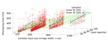
Figure 4: Example of 2D and 1D linear fitting of processing data values in the dispatcher, for each computer $k$ and lambda function $j$.

If the assumptions in this section do not apply to a specific scenario, for instance the execution time does not correlate to the input size, then another processing time estimation algorithm (e.g., one more sophisticated or that has white-box knowledge of the applications or computers) can be plugged in seamlessly when implementing the edge dispatching, without affecting the overall framework proposed.

3.2.3 Overall dispatching algorithm

To summarize, every time a lambda function $j$ of size $S_{j}$ is correctly executed by computer $k$, which reports load $u_{k}$ and processing time $p_{jk}$, the dispatcher performs the following house-keeping operations:

1. measure the communication latency $\tau_{jk}$ as the difference between the overall lambda execution time, which is a local information, and $p_{jk}$;

2. add $\{S_{j}\rightarrow\tau_{jk}\}$ to a moving window of $W_{\tau}$ samples and find the intercept/slope values $\alpha^{\tau}_{k}$/$\beta^{\tau}_{k}$ that best fit them;

3. quantize $S_{j}$ as $S^{\prime}$ to the closest value among the $W_{S}$ possible ones;

4. add $\{u_{k}\rightarrow p_{jk}\}$ to a moving window of $W_{p}$ samples and find the intercept/slope values $\alpha^{p}_{S^{\prime}jk}$/$\beta^{p}_{S^{\prime}jk}$ that best fit them.

By design, measurements are always collected as the result of the dispatching algorithm selecting a computer as the destination of a lambda function execution request. This sort of passive polling guarantees high scalability as the number of computers and dispatchers grows, but it has a side effect possibly leading to sub-optimal selection: once a computer becomes affected by a bad reputation due to possibly temporary overload conditions, either due to concurrent tasks or network traffic, such a status may never be cleared because the dispatcher is unlikely to select it as the best choice. To prevent such a starvation, we associate a lifetime to the measurements: after a timeout $T_{\tau}$ ($T_{u}$) the values collected regarding the communication latency (processing time) estimation process are discarded, and the computer’s state is restored afresh as if it had just entered the edge computing domain. In a production environment where an optimization process adapts the computational/networking resources over time, the lifetime-based approach could also be substituted by an event triggered on the dispatchers by the orchestration layer.

The final dispatching algorithm for an incoming lambda function of type $j$, whose input is $S_{j}$, quantized as $S^{\prime}$, consists of finding the destination computer $\bar{k}$ s.t.:

$$\bar{k}=\arg\min_{k}\left\{\left(\alpha^{\tau}_{k}+\beta^{\tau}_{k}S_{j}\right)+\left(\alpha^{p}_{S^{\prime}jk}+\beta^{p}_{S^{\prime}jk}u_{k}\right)\right\}$$ (3)

To achieve high scalability with non-specialized hardware, it is important that the dispatching algorithm remains as simple and fast as possible as the number of computers and lambda functions grow. The worst-case computational complexity, in both space and time, of the main algorithm components is reported in Table 2, where the house-keeping rows refer to operations that are carried out upon receiving a successful response from a computer. We briefly recall the notation used in the table: $L$ is the number of possible lambda functions, $C$ is the number of computers in the edge network, and $W_{\tau}$, $W_{S}$, and $W_{p}$ are the internal parameters representing the number of communication latency samples kept per computer, the number of quantized input sizes, and the number of processing times kept per lambda per computer, respectively.

Table 2: Computational complexity analysis.

Algorithm	Space	Time
Communication latency house-keeping	$\mathcal{O}(W_{\tau}C)$	$\mathcal{O}(W_{\tau})$
Processing time house-keeping	$\mathcal{O}(LW_{p}W_{S}C)$	$\mathcal{O}(W_{p})$
Dispatching	–	$\mathcal{O}(C)$

On the other hand, to quantify the average computational complexity of the algorithm we have carried out the following testbed experiments. We have run a single instance of a dispatcher, whose internal structure and implementation details are illustrated in Sec. 4.4, on a Raspberry Pi 3 Model B (RPi3), which is “representative of a broad family of smart devices and appliances” [35], and on an Intel application server with Xeon CPU E5–2640 v4 at 2.40GHz. Even though the application can exploit parallelism on Symmetric Multiprocessing (SMP) architectures by spawning multiple threads, for the purpose of the experiment we have restricted the execution on a single core. In the experiment we have installed a given number of possible destinations of a special lambda, for which the dispatcher replies immediately to the client without actually reaching a computer. However, all other phases of the dispatching algorithm, including the computation of Eq. (3) and the update of all the internal data structures and timers, are performed exactly as with regular lambda functions. We have run experiments with 1 and 4 threads spawned in the dispatcher, and executed a matching number of clients repeatedly asking for the special lambda function to be executed.

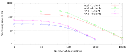
Figure 5: Dispatcher processing rates.

In Fig. 5 we report the processing rate achieved in the different combinations, which gives an upper bound of the performance of the dispatcher (per single core) and a quantitative measure of the computational cost of the proposed algorithm as the number of destinations ($C$) increases. For each combination of parameters we have executed 10 repetitions, but we do not report error bars in the plot because the variance was negligible. As can be seen, in all cases the processing rate decreases linearly in the log-log plot, which means that the average computational complexity increase w.r.t $C$ is sub-linear, unlike the worst-case computational complexity, which is in fact often considered too pessimistic. This provides for a smooth scalability of the dispatcher as the edge computing size, i.e., the number of computers, increases. In absolute terms, the Intel server-grade CPU obviously performs much better than RPi3’s ARM CPU, and achieves a processing rate significantly greater than 1000 Hz, which means less than 1 ms overhead per function call, with up to 10,000 possible destinations. However, also the RPi3 incurs a reasonable small overhead in a range that is certainly relevant for many practical deployments.

In the supplementary material we also include the CPU utilization measured during the experiments.

4 Simulation framework

As illustrated extensively in Sec. 2.3, to the best of our knowledge, the existing solutions to evaluate the edge computing performance have some limitations when realistic modeling of both connectivity and computation is required. In this section we propose a novel framework that overcome these limitations. The framework has been developed originally for the performance analysis of the serverless edge computing architecture described in Sec. 3, but it can be used “as is” for the evaluation of generic algorithms and protocols in a wide range of scenarios.

Our solution builds on network emulation and lightweight virtualization, combined with simulation of the computation processes. Therefore, all system components are instanced as Linux applications running inside lxc containers, which is a form of process-based virtualization, incurring a negligible overhead compared to running the same application on the host OS. This allows the experimenter to take into account in a realistic manner all the effects due to the communication protocols in use, as well as including in the analysis several phenomena that are very difficult to capture using simulators, e.g., inter-process communication overhead and caching. Furthermore, network emulation can be realized efficiently using mininet, which is known to scale well to large topologies with thousands of nodes on a single server.

The use of real components in experiments, however, does not mean that necessarily all applications must be real ones. In fact, we argue that in many cases the use of real edge applications is not needed. This is the case of our distributed dispatching system for serverless edge computing, described in Sec. 3, which focuses on the forwarding of the functions, but it is agnostic of the actual applications being run by the clients. Since edge applications are very likely to be a choke point for the execution of large scale experiments, because offloading is especially appealing for computationally-intensive tasks that cannot be executed efficiently on devices, by simulating computation we can retain all the advantages of a real testbed with a fraction of the hardware required. This, in turn, opens the door to easy automatization of the execution of the experiments, simplified collection/analysis of results, and straightforward repetition of experiments.

In the remainder of this section we first describe the experiment workflow (Sec. 4.1) and the computation element simulation model (Sec. 4.2), which are both general and application-agnostic. Afterwards we focus on the serverless-specific components of our framework: we illustrate the image manipulation computer (Sec. 4.3), used in Sec. 5 directly, i.e., instances are executed as part of the experiments, and indirectly, i.e., to calibrate the configuration parameters of the computation element simulation model, and finally the serverless edge computing dispatcher (Sec. 4.4).

4.1 Experiment workflow

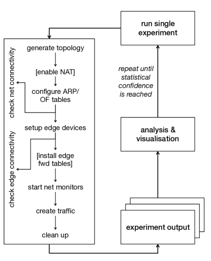
Figure 6: Workflow of a generic experiment.

In Fig. 6 we illustrate the generic experiment workflow: the execution of a single experiment is done by launching a Python script, which includes a number of generic modules developed as part of our framework, interacting with mininet via a Python API. The modules implement the logic to realize all the steps reported in the left hand side box in Fig. 6, including the topology generation according to models suitable for edge computing environments and the configuration of the OpenFlow (OF) and Address Resolution Protocol (ARP) tables in switches to ensure network-layer connectivity. Every intermediate step may be customized by the experimenter by overriding the relevant methods of the main experiment class to suit their specific needs. Common-use metrics, such as per-switch throughput, are collected by default and made available at the end of the experiment, together with custom metrics. The analysis and visualization of the experiment output is instead beyond the scope of the framework, since it ultimately depends on the actual environment.

Our framework is general enough that it can be used to simulate a multitude of different edge computing environments, also including interactions with real world applications living outside the virtualized mininet environment through an appropriate Network Address Translation (NAT) configuration. We have used the framework to validate and assess the performance of our distributed architecture for serverless edge computing with real and simulated computation elements, in a vast range of network topologies, using different methodologies (transient analysis, steady-state with replications, Monte Carlo).

4.2 Computer simulation model

We now present the model of the simulated computer, which is an application that performs arbitrary functions without really implementing any algorithm, but rather simulates internally the execution of the currently scheduled lambda functions to mimic the behavior of an SMP multi-container edge server. Tasks are served according to a First Come First Serve (FCFS) non-preemptive policy. Every task is associated to requirements in terms of both computation (number of operations) and memory (bytes). In the simulated computer implemented we have used a linear model where the number of operations (or memory) required is the sum of a constant offset and a value that is proportional to the input of the lambda function request, in bytes. In the supplementary material we show that this model is able to capture very well the response time of the image manipulation computer described in Sec. 4.3. Different offset/slope values can be used for different lambda functions in different computers: this allows to simulate computers that have heterogeneous characteristics, such as equipped with GPUs/ Vision Processing Unit (VPU) better suited to graphics/ML jobs than general-purpose CPUs. The number of operations is used to determine the simulated processing time, which also depends on the number of cores and the CPU speed. Multiple tasks can share the available cores, provided that the container on which they are running have sufficient workers available, otherwise the tasks are put into a waiting list. On the other hand, the memory required is used to block tasks whose requirement would exceed the residual memory available, which is the difference between the total amount installed (in simulation) and the sum of the memory requirements of all active tasks. If a task is blocked because of insufficient memory, no other task is put into execution until it is eventually made active, to avoid starvation. Different models to compute the computation/memory requirements, as well as different scheduling policies, can be easily implemented, should they be needed to better model a given platform or application under evaluation.

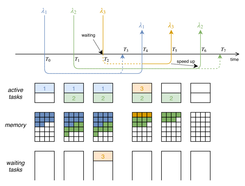
Figure 7: Example of processing simulation.

To better explain the behavior of the simulated computer we now illustrate two example simulations, both with three incoming tasks. For simplicity we assume there is a single simulated core. All the lambda functions are served by the same container, i.e., they are of the same type, with two workers. In the first example, in Fig. 7, memory is not a limitation and it is not considered (it is the subject of the second example). At $T_{0}$ the first task $\lambda_{1}$ enters the system; based on its input size and the offset/slope configured for this container in this computer, the completion time $T_{3}$ is assigned: if no other tasks arrived, that would be the time when $\lambda_{1}$ returns. However, at $T_{1}$ a second task $\lambda_{2}$ arrives: in addition to assigning a completion time to it ($T_{7}$), the simulated computer also modifies the completion time of $\lambda_{1}$ to $T_{4}$ because from now on it has to share CPU cycles with $\lambda_{2}$. When a third task $\lambda_{3}$ arrives, it is put into the waiting list because there are no workers available; this situation changes only as $\lambda_{1}$ leaves the system, when $\lambda_{3}$ is put immediately into execution: note that the completion time of $\lambda_{2}$ which is still active, does not change because the number of active tasks remains the same. On the other hand, as $\lambda_{3}$ completes its execution, $\lambda_{2}$ becomes the only active task, which makes the computer shorten its completion time from $T_{7}$ to $T_{6}$.

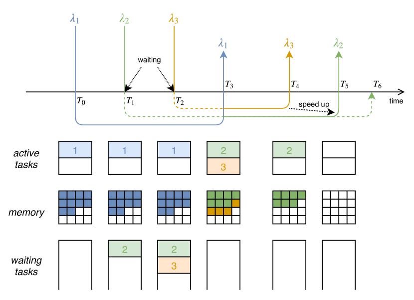
Figure 8: Example of processing simulation, with memory-bound tasks.

In the second example, in Fig. 8, the tasks have exactly the same characteristics and arriving times, but we now have a smaller memory. Because of this tighter constraint, as $\lambda_{2}$ arrives at $T_{1}$, it cannot be made active because memory is insufficient. Therefore it is put into the waiting list, while $\lambda_{1}$ enjoys full CPU power, hence no completion time advance like in the first example. When $\lambda_{3}$ arrives at $T_{2}$, its memory requirements would fit into the residual capacity, but it is put into a waiting list together with $\lambda_{2}$ because we enforce a FCFS policy. As already mentioned, this also automatically avoids starvation of tasks with large memory requirements. As soon as $\lambda_{1}$ completes at $T_{3}$, both waiting tasks become active, and the simulation then proceeds as in the first example.

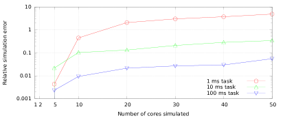
Figure 9: Relative execution error of the computer simulator as the number of simulated cores increases.

Quite clearly, since the simulation must happen in real-time, there are limitations to the processing rates that can be achieved by the simulated computer. We now show in a quantitative manner, with the results from an experiment, that the range of operation of the simulated computer are very reasonable. We run an instance of a simulated computer on a single core of an Intel Xeon CPU E5–2640 v4 at 2.40GHz (same machine used for the dispatcher results in Sec. 3.2.3 above and for the experiments in Sec. 5 below). We are interested into measuring the error introduced by the simulated computer as a function of: the number of cores simulated and the processing rate. To this aim, we set up a number of clients equal to the number of simulated cores, continuously requesting the execution of a lambda function configured with offset/slope such that its processing time is 1 ms, 10 ms, and 100 ms, respectively. Memory limits do not constrain execution of applications. In these conditions, we expect that the response time will be exactly the same as the nominal processing time, because every task has a dedicated simulated container/core for its execution: every deviation is due to the physical CPU of the host not being able to keep the pace with the simulated events. In Fig. 9 we plot the relative execution error, defined as the ratio between the actual processing time and the expected processing time minus 1. Since the actual processing time is always greater than the expected value, because a CPU may only lag in time, the relative execution error is always positive: for instance a value of 0 means that there is perfect match between simulated and actual processing times, whereas a value of 0.1 means that the computer is introducing an error in the order of 10% of the processing time. In the supplementary material we also report the physical CPU utilization during the whole experiment. As can be seen in the plot, a single physical core is able to simulate with small error a server equipped with many cores, up to 50 in our experiments, provided that the processing time is 10 ms or higher. For instance, this means simulating $50\times 20=1000$ containers on the server we have used, which has 20 physical cores. On the other hand, if simulation with fine-grained granularity of a multi-core machine serving such shortly-lived tasks is required, it will be necessary to allocate sufficient physical CPU cores to the computers to obtain accurate results at high processing rates.

As already introduced, this simulated computer is very important for performance evaluation purposes: (i) it allows to scale experiments up to large networks without requiring prohibitive computational capabilities, (ii) it enables the execution of sensitivity analysis studies, having a totally known and controllable response, and (iii) finally it allows the implementation of the comparison algorithm proposed in [6] because it can predict the completion time of jobs (if no other arrives meanwhile).

4.3 Image manipulation computer

In addition to the simulated computer described above, for the purpose of evaluating our serverless edge computing architecture with a realistic application of practical interest, i.e., mobile AR, we implemented an image manipulation computer that actually performs face or eyes detection using the OpenCV library. This also shows how our performance evaluation framework can work with real applications, simulated ones (as described in Sec. 4.2 below), or any mix of the two. However, we are not interested in the details and challenges associated to the specific detection algorithms, for which we refer the interested reader to, e.g., [36].

The OpenCV library is able to use concurrently multiple CPU cores to reduce the processing time. The maximum concurrency level can be set at run-time, and in the experiments we use this feature to artificially limit the computational capabilities of computers.

With regard to face detection, the edge client on the device sends a picture to the dispatcher selecting face_detection as the lambda name. The dispatcher then forwards the request to a suitable computer, which replies with the rectangles enclosing all the faces found, if any. The response time is the time between when the edge client issues the lambda request and when it receives back the response. If detection of eyes is also requested, then the edge client, for every face found in the first step, crops the original image based on the rectangle coordinates and issues another lambda request of type eyes_detection, which is also dispatched as before to a suitable computer. In this case the response time is measured by the client between when the initial face detection is requested and when the last eyes detection response is received.

Table 3: Response times of the lambda functions used in the experiments with an image manipulation computer for face detection.

Picture size	Size (bytes)	Comp. only (ms)	With network (ms)
320$\times$240	52830	43 $\pm$ 9	60 $\pm$ 10
640$\times$480	175332	101 $\pm$ 10	218 $\pm$ 26
960$\times$720	353230	181 $\pm$ 13	446 $\pm$ 47
1280$\times$960	560103	301 $\pm$ 13	744 $\pm$ 45

We report in Table 3 the response times of face detection with the set of pictures used in the performance evaluation, ranging from 320$\times$240 to 1280$\times$960, when using up to two CPU cores. We report the times both when called directly (Comp. only column in the table) and when the lambda function is invoked by a client to a computer via a network link (With network column in the table) emulating a typical WLAN access network. The variance of results is rather high due to the ML algorithm used in the OpenCV library for detection.

4.4 Dispatcher prototype

Figure 10: Finite state machine of a dispatcher.

We conclude this section by describing the online lambda function dispatcher implemented in our framework, which can be represented using the Finite State Machine (FSM) in Fig. 10. As illustrated, the dispatcher continuously waits for new lambda execution requests from clients. Once a new one arrives, one of the idle handlers takes care of its entire execution until a response is returned to the client before it can be considered idle again. A handler initially selects the destination based on Eq. (3), then forwards the lambda request to the computer selected and waits from a response, which is eventually forwarded to the client. Afterwards, the handler uses a locally measured delay together with the processing time and load indication piggybacked by the computer on the response to perform the so-called house-keeping operations in Sec. 3.2.3. Both the latter and destination selection use data structures that are in common for all the handlers, which may limit in principle the degree of parallelism that can be achieved as the number of handlers is increased, especially for lambda functions with a short execution time.

We implemented the dispatcher in C++ and the execution of lambda functions has been realized by means of REST interface methods using Google’s gRPC, which is a mature industrial-grade communication protocol using Hyper-Text Transfer Protocol (HTTP), with messages serialized with Google’s protobuf library, which is lightweight and portable. A lambda request contains: the name, that is used to identify the container or run-time environment to be used; the input, that is opaque to the edge computing components ; and a flag that, if enabled, tells the dispatcher not to actually forward the lambda but reply immediately with an estimate of the time it would be required to carry out the function. This last field could be used by a client associated to multiple dispatchers to decide where to request execution. Think for instance of a user with a smart phone connected to a mobile network and a WLAN, both offering edge computing services. A lambda response contains: a return code specifying what went wrong, if anything; the output; the Uniform Resource Locator (URL) of the computer actually carrying out the computation; the time required for the execution of the lambda; the response, opaque to the edge computing components; a short-term average load of the computer before the execution of the lambda function.

In the prototype, our applications, written in C++, call directly the REST methods on the dispatcher to which they are attached, but integration with any other high-level programming language is possible since the gRPC library is platform and language independent. To simplify the discovery phase, we assumed that every computer and dispatcher registers itself to the controller at a known URL. Finally, to achieve interoperability in a real deployment we envisage adopting standard APIs, such as those defined by the ETSI MEC [37]; such an opportunity is being currently investigated.

5 Performance evaluation

In this section we evaluate the distributed lambda dispatching algorithm with the proposed performance evaluation framework in three setups: an artificial scenario in Sec. 5.1, configured in different flavors to show the flexibility of our simulation framework to model very heterogeneous conditions, as well as to introduce the main characteristics of the proposed distributed dispatching algorithms; a small-scale network of edge nodes, equipped with real face detection capabilities in Sec. 5.2 (this set-up is also used for an assessment of the sensitivity of results to the main internal parameters in Sec. 5.3); a more realistic large-scale environment where we have used simulated computers (Sec. 5.4).

The experiments have been run on a Linux Intel Xeon dual socket workstation, with Intel Hyper Threading disabled, that was not used by any concurrent demanding application. During all the experiments the computational processing demands were never significant enough to suggest that the results might be affected by a hardware limitation of the host used. In all the experiments we have used $W_{\tau}=W_{p}=100$ based on preliminary calibration experiments: we do not report these results because they would give the reader little insight, however we have verified a posteriori, using the method of $2^{k}r!$ analysis [38], that the results are not affected, in a statistical sense, by setting these parameters to 50% and 200% of the value above, see Sec. 5.3 below for full details. The value of $W_{S}$ depends on the specific experiment and is indicated in the respective sections below. Unless otherwise specified, every experiment has been repeated 10 times: in the plots we report the 95% confidence interval over all the replications.

For all the scenarios below, additional results are available as part of the paper supplementary material.

5.1 Exploring resource limitations

Figure 11: Network topology used in the resource limitations experiments.

In this section we show that our proposed framework can adapt to a wide range of environments: as described in Sec. 4 this is very important for the performance evaluation in edge computing environments, since the latter span across several markets / vertical industries, each with very specific and heterogeneous characteristics. We use the simple network topology illustrated in Fig. 11, in which the thick edges have 100 Mb/s bandwidth / 1 $\mu$s latency, and they connect a root node (also hosting the controller) to the edge nodes, whereas the thin edges have 25 Mb/s bandwidth / 100 $\mu$s latency, connecting the clients to their respective edge nodes. The left-hand-side (LHS) computer offers serverless functions $\lambda_{1}$,$\lambda_{2}$ and the right-hand-side (RHS) computer offers $\lambda_{2}$,$\lambda_{3}$; every client issues lambda function requests of the same type indicated in the figure: as a result of these assumptions, the so-called interfering clients on the left and right of the network may be served only by their respective computers, while the tagged client in the middle has its requests served by the LHS or RHS computer depending on the decisions of its dispatcher.

We have configured the computers to give the same response times, on average, as a real image manipulation computer for face detection, reported in Table 3. The tagged client issues lambda request with size corresponding to a 320$\times$240 picture every 200 ms on average (actual inter-time between consecutive requests is drawn from a uniform r.v.); on the other hand, the interfering clients, when present, use all possible picture sizes in the table with an average inter-time of 1 s. We simulate four cases: (i) Baseline: without interfering clients, only to establish a reference of the performance metrics; (ii) CPU: we make the two computers unbalanced in terms of computation power by reducing to $\frac{1}{3}$ the number of RHS’s simulated cores; (iii) Memory: we make the two computers unbalanced in terms of memory by specifying a limited memory for RHS, while the memory of LHS never constrains execution of tasks in this scenario; (iv) Network: we simulate background traffic between the root node and the LHS Computer by transmitting bursts of TCP exchanges lasting for 3 s every 5 s.

In all the four cases we compare the following schemes:

Probe

(inspired from [6]): a centralized dispatcher co-located with the controller polls each computer to retrieve the execution time required, then selects the one that advertised the smallest value; the implementation of Probe with simulated computers (see Sec. 4.2) is straightforward since they always know precisely the execution time of any incoming task, provided that no other jobs arrive.

RPI

(Relative Performance Index, inspired from [39]): the dispatcher uses a Weighted Round Robin (WRR) scheduler to select the destination of incoming lambda function requests, with the weight being equal to its zero-load response time, normalized in range whose bounds are given by the fastest and slowest computer, respectively; the weights are computed in an initial profiling phase during which the dispatcher executes every lambda function on every computer, while no other task is being executed on it.

Est

: our proposed dispatching algorithm described in Sec. 3.2.3.

Clearly, both Probe and RPI cannot be implemented in a real deployment and they are to be considered only as optimistic performance reference: on the one hand, Probe requires the execution time of any task to be known a priori, but this information is generally not available; on the other hand, the initial profiling of RPI requires that the edge computing system is unavailable throughout this phase, which may be unfeasible in a live system.

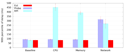
Figure 12: Resource limitations: 90th percentile of delay.

In Fig. 12 we show the 90th percentile of the delay, which is defined as the time between when the client issues a lambda request and when it receives the response from the dispatcher. In the Baseline case the delay is the same for RPI and Est, but slightly greater with Probe, due to the additional delay of polling the computers to check which one would provide the shortest processing time. In the CPU and Memory cases, the 90th percentile of delay increases significantly with RPI because the latter blindly balances between the two computers, regardless of their current state. On the other hand, our proposed dispatching algorithm, using only local estimated information, is as efficient as a centralized version that uses reliable information from the computers themselves. In the Network case, Est outperforms both comparison schemes since it also includes in its algorithm (see Eq. (3)) the communication latency.

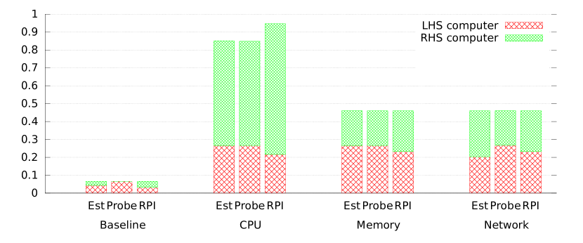
Figure 13: Resource limitation: average load.

In Fig. 13 we provide additional insight on the system dynamics by showing the average load of the computers, defined as the fraction of time that the simulated cores are actively processing tasks. First, we note that with Baseline the Probe scheme uses only one computer: since they are identical and there are no other clients than the tagged one competing for resources, polling deterministically returns the same value on both computers. Second, in the CPU case, the RHS load is higher because it has less simulated computational resources. Finally, in the Memory and Network cases, the LHS computer’s load is respectively the same with both Probe and RPI: this is because both solutions take into account only the processing time, either statically identified in a profiling phase or dynamically requested from the computers, which yields worse performance than Est, which instead is more flexible in adapting to the different computational capabilities and serverless/background traffic conditions.

5.2 Small-scale experiments

In this set of experiments we arranged four edge nodes interconnected in a clique with 100 Mb/s links with 1 $\mu$s latency. This is representative, for example, of a local edge environment supporting a group of mobile nodes, deployed by a MEC operator through a set of edge gateways located close to each other. Each edge node hosts an image manipulation computer that can perform face detection via the execution of lambda functions as described in Sec. 4. The computers are assigned different capabilities: the computer on node $i$, with $i\in[1..4]$, can use up to $i$ CPU cores among those available in the server hosting the experiments. All clients connect to the edge nodes via links with 25 Mb/s capacity with 100 $\mu$s latency. For the convenience of evaluation we measure the latency of “tagged” clients only, one per edge node, that issue, on average, one lambda request per second with picture size 640x480 pixels according to a Poisson distribution. The number of other clients, requesting detection on pictures randomly drawn from a set of images from 320x240 to 1280x768 pixels and roaming from one edge node to another selected randomly, increases from 1 to 4. In these experiments it is $W_{S}=4$.

Figure 14: Network topology used in the small-scale testbed experiments.

We compare the performance obtained with our proposed dispatching solution, called Est in the following, with two alternative approaches. First, a Round Robin (RR) algorithm, taken from our previous work [40], which classifies the computers based on lower vs. higher response time, then dispatches the incoming lambda request to the computers that are currently in the lower category. RR does not distinguish between communication and processing delays and does not use the load values reported by the computers. Second, we consider a Legacy approach, where the clients simply request the execution to the closest computer, in number of hops.

In Fig. 15 we show the 90th percentile of the delay of tagged clients. As can be seen, at low network loads RR performs worse that the others, because it strives to use evenly the available computers, which however have different capabilities. This behavior pays off at high loads, where, on the other hand, Legacy is penalized because it cannot cope well with “hot spots” of clients. In all cases the Est curve lies always below the others: our proposed approach can adapt well to mixed environments. Recall that this is achieved in a fully distributed manner and without providing Est with any a priori knowledge on the topology and capabilities of computers.

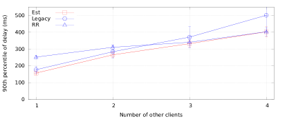
Figure 15: Small-scale experiment: 90th percentile of delay.

The reason is explained with the use of Fig. 16, which shows the average load of the computers at peak load. As can be seen, Legacy has an almost flat utilization, which is inefficient since the load is evenly distributed across edge nodes but the capabilities are not. Note that a condition of unbalanced capabilities is far from being artificial: rather, in a real environment it is very likely that hardware and software on edge nodes, unlike their cloud counterparts, will be highly heterogeneous due to incremental deployment and fragmented ownership. On the other hand, both Est and RR distribute the load proportional to where there are more resources. For instance, even though computer 1 has lowest capabilities, it has non-negligible utilization with Est, which is thus able to harvest resources even from less powerful computers as necessary.

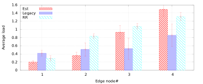
Figure 16: Small-scale experiment: Distribution of load across edge computers, with four other clients.

5.3 Sensitivity analysis

In this section we study the sensitivity of the proposed dispatching algorithm to variations of its internal parameters. We carry out this analysis using a $2^{k}r!$ analysis, which is an established methodology to identify the dominant factors in a statistically sound manner and, usually, plan experiments accordingly. Very briefly, for each of the $k$ factors potentially affecting the performance, we identify two limit cases, identified by a $+$ and $-$ sign, respectively. Then, we run $2^{k}$ experiments in all possible combinations. We also repeat $r$ times every experiment, without modifying the parameters. For every metric of interest, the $2^{k}r!$ method allows to derive the relative importance of every factor or combinations of factors, also quantifying the contributions in the same units as the performance index under study, within a given confidence interval. One basic assumption for this method to provide meaningful results is that the factors identified give additive contributions to the metric of interest (though the analysis may still be carried out with non-additive contributions with some modifications). The interested reader may find additional information on this methodology in [38].

Table 4: Sensitivity $2^{k}r!$ analysis: factors.

Parameter		$-$	$+$
Number of other clients	A	1	4
$T_{\tau}$	B	1	10
$T_{u}$	C	1	10
$W_{\tau}$	D	50	200
$W_{u}$	E	50	200
Detect eyes	F	no	yes

The sensitivity analysis is carried out in the same topology as Sec. 5.2. The $k=6$ factors identified are reported in Table 4 and they include internal parameters ($W_{\tau}$, $W_{u}$, $T_{\tau}$, $T_{u}$, see Sec. 3.2.3) as well as the following environmental parameters: the number of other clients, which is basically a measure of the computational/network load; and whether the serverless clients request only face detection or also the detection of eyes within every face found in the pictures. In the latter case all the computers offer two lambdas, one for face and the other for eyes detection, and the delay is the response time defined in Sec. 4.3. We performed the analysis in terms of the following metrics: delay, network throughput, load of the computers, and communication latency/processing time estimation error, defined as the absolute value of the difference between the a priori estimation and the a posteriori measurement done by the dispatcher for every lambda function. We run 10 independent replications for every combination of parameter, i.e. $r=10$, yielding a total of $2^{6}\cdot 10=640$ experiments executed.

Table 5: Sensitivity $2^{k}r!$ analysis: 90th percentile of delay (ms).

Effects	Contribution	Conf. int.
mean response (q0)	$342$	$(340,343)$
effect of A (qA)	$+75.6$	$(73.7,77.5)$
effect of F (qF)	$+43.4$	$(41.5,45.3)$
other effects	negligible
unexplained variations	9%

In Table 5 we show the analysis in terms of the 90th percentile of delay, produced by the open source tool factorial2kr used. Confidence intervals are computed with 95% level. From the table we see that the 90th percentile of delay is affected merely by environmental parameters A (number of other clients) and F (detection of face only vs. face+eyes). The sign of the qA and qF values also gives us the direction, which is as expected: the latency increases as the number of other clients increases from 1 to 4 (the average increase is 75.6 ms) and if we also include eyes detection (the average increase is 43.4 ms).

Table 6: Sensitivity $2^{k}r!$ analysis: median of processing time estimation error (ms).

Effects	Contribution	Conf. int.
mean response (q0)	$22.2$	$(21.8,22.6)$
effect of A (qA)	$+13.4$	$(13.0,13.8)$
effect of F (qF)	$-19.7$	$(-20.1,-19.3)$
joint effect of A&F (qAF)	$-12.6$	$(-12.9,-12.2)$
other effects	negligible
unexplained variations	4%

In Table 6 we report the analysis when considering the processing time estimation error $|\hat{p}-p|$. As for the 90th percentile of delay, only the environmental factors have non-negligible impact on the performance. However, there are two differences. First, the sign of qA and qF is opposite, which means that in this case the processing time estimation errors increases as the load increases, but it decreases if the clients also perform eyes detection. This is an effect due to the shorter duration of eyes detection compared to face detection, because when requesting the latter the clients only include as input the portion of picture corresponding to a single face. Second, a combination qAF appeared in the table: this means that 21% of the processing time error is due to the joint effect of the number of other clients and application of choice, which can be explained by the fact that having more serverless traffic also gives more measurements to the dispatcher, which can then be more precise in their estimations, especially with faster detection algorithms.

For all the metrics considered, we have verified that the results are valid in a statistical sense by visually inspecting the residual errors, whose residuals vs. predicted values and Q-Q normal plots are reported in the supplementary material.

5.4 Large-scale topology

In this section we report the results obtained with a large-scale realistic network topology, where lambda functions are executed on simulated computers. The target application is AR on mobile devices in a dense urban environment. We use as reference real-world traces available as open datasets and described in [41], which include recordings of human activity in the city of Milan (Italy) for one month. The city landscape is divided into a square grid of 10,000 cells. We assume that each cell contains a base station serving users divided into three sectors. Base stations are grouped into sets of three elements, forming so-called pods, that are then connected to a common core. The resulting network topology is a fat-tree, commonly found in data-centers and operator core networks [42], where the network links between the root node and its children have 1 Gb/s with 10 $\mu$s latency, whereas capacity is halved in the tier below. The links connecting the clients to their respective base station have a 25 Mb/s capacity with 1 ms, which is a slightly optimistic estimate with respect to actual findings in current 4G networks [43]. The mapping of the city grid into an emulated network for the experiments is illustrated in Fig. 17. In particular, the network view (right side) shows the connectivity graph, where the thickness of the edge is a qualitative indicator of the link speed: at the terminals level, one node represents all the user terminals in a sector; at the base stations level, one node represents a single (sectorized) base station, which acts as both a dispatcher and a computer, with two cores entirely dedicated to processing lambda functions; at the pods level, one node represents the collection of networking equipment creating a backhaul connection between the access and core networks; finally, the entire core network is collapsed into the root node of the tree.

Figure 17: Mapping of the city grid from [41] into the network topology used for the experiments.

For the experiments we used a Monte Carlo approach, which is widely employed for system-level performance evaluation of MBWA algorithms and protocols and is carried out as follows. Inspired from the evaluation in [44], from a random day in the dataset in [41] we extracted Internet activity with a 10-minute granularity, that is used to determine the cell load at every given time of day. Then, we perform a number of independent snapshots (or drops) of the system. For each snapshot we select a random location of a group of 3x3 cells and a random time of day. Then, we drop users with random arrival times with a rate that is proportional to each cell activity at the given time. Each user establishes a session of AR with a duration randomly extracted between 30 s and 60 s, consisting of a stream of lambda function requests directed to the dispatcher co-located with the serving base station. During a session, consecutive lambda functions are issued every 33 ms, which corresponds to a frame rate of 30 fps. The size of lambda requests/responses is such to have bandwidth demands ranging from 3 Mb/s (lambda size 5000 bytes) to 10 Mb/s (lambda size 15000 bytes), which according to the authors in [45] is a reasonable compromise for good quality AR under realistic network constraints. The response times of the lambda function with some image sizes are reported in Table 7. We consider 75 ms as the maximum tolerable round-trip delay for the execution of a lambda function [45]. In the dispatchers we used a value of $W_{S}$ such that lambda sizes are quantized every 1000 bytes.

Table 7: Response times of the lambda functions used in Sec. 5.4 with a simulated computed emulating an AR application.

Size (bytes)	Comp. only (ms)	With network (ms)
5000 bytes	9.0 $\pm$ 0.2	12.1 $\pm$ 0.4
10000 bytes	17.5 $\pm$ 0.2	24.1 $\pm$ 0.3
15000 bytes	25.9 $\pm$ 0.2	35.9 $\pm$ 0.5

We compare our proposed solution, called Dist Est (= distributed with processing estimation) below, to the following alternatives. First, a centralized approach where the dispatcher is located in the root node of the topology tree, which mimics the behavior of a typical serverless solution, such as OpenWhisk. Second, a distributed version of the Probe algorithm, hence called Dist Probe, described in Sec. 5.1. Third, like in Sec. 5.2, Legacy, where the clients request the execution of lambdas to their serving base station.

In Fig. 18 we report the 90th percentile of the delay experienced by the fraction of users in the x-axis. For instance, with Dist Est we have a value of 40 ms at 0.7 users: this means that 70% of the users, at every random location and time of day, experienced a 90th percentile of delay that is smaller than 40 ms. Therefore, we can compare these values to the 75 ms target and find the fraction of dissatisfied users as the complement to 1 of the x-axis projection of the point where each curve meets 75 ms. In this respect, Legacy achieves poorest performance: this is because a static allocation leads to under-utilization of the computational resources, which is consistent with the main finding in [46]. This is mainly due to the fact that with Legacy we create “hot spots” of requests at each base station whenever a high concentration of clients appears at that base station. Instead, Dist Est achieves roughly the same performance as Centralized, which however suffers from a slightly higher number of dissatisfied users because of the inconvenience of forcing all the transactions to pass through the root node, i.e., the core network, which is more prominent at high loads. Finally, Dist Est enjoys smaller delays than Dist Probe in almost all cases, but the performance gap lessens as the load increases. In particular, the fraction of dissatisfied users for the two algorithms is the same, though Dist Probe incurs a much more exorbitant cost in terms of network consumption, as discussed below.

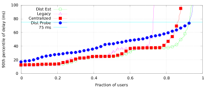
Figure 18: Large-scale experiment: Distribution of the 90th of delay.

This effect of excessive resort to network, which negatively affects the delay performance, is shown directly in Fig. 19, which reports the overall average per-drop network throughput, sorted on the y-axis values. Clearly, Legacy has minimum network consumption because the computation offloading traffic never leaves the base station. However, as can be seen, the network overhead caused by Dist Est with respect to Legacy is negligible compared to that of both Centralized and Dist Probe. This confirms that our proposed dispatching algorithm is able to achieve a good trade-off between wise utilization of the computational resources available and protocol/architecture complexity to achieve this goal, which ultimately benefits application latency in addition to traffic exchange.

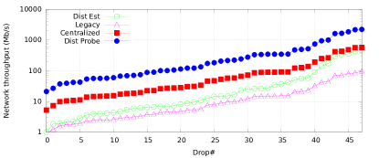
Figure 19: Large-scale experiment: Network throughput per drop.

6 Conclusions

In this paper we have proposed a system to offload pervasive applications with stringent delay requirements as stateless functions on edge nodes with available computational capabilities, called computers. The execution of functions passes through edge nodes with dispatching capabilities, which are ideally located as close as possible to the final users. The proposed architecture is highly scalable as the number of both the clients and the computers grow because of its distributed nature, in fact all edge nodes use only local information to dispatch lambda functions, and thanks to the dispatchers only performing passive measurements to estimate the communication and processing times.

Furthermore, to overcome the limitations of existing frameworks for the evaluation of edge computing systems, we have devised a novel approach that jointly exploits network emulation, process-based virtualization, and simulation of computation tasks to obtain accurate results in controlled repeatable conditions with reasonable computation effort. We have used our framework to validate the distributed algorithm to dispatch lambda functions in several scenarios. The results have shown that the proposed distributed architecture performs much better than statically allocating clients to computers and the same as or better than both a centralized approach and a distributed comparison solution from the literature.

As future work, we will work on the integration of our performance evaluation framework with edge computing platforms and communication stacks to take into account in a realistic manner the overhead and complexity introduced by, e.g., the ETSI MEC or the LTE Evolved Packet Core (EPC).

References

- [1] M. Satyanarayanan, The Emergence of Edge Computing, Computer 50 (1) (2017) 30–39. doi:10.1109/MC.2017.9.
-
[2]
C. Li, Y. Xue, J. Wang, W. Zhang, T. Li,
Edge-Oriented
Computing Paradigms, ACM Computing Surveys 51 (2) (2018) 1–34.
doi:10.1145/3154815.
URL http://dl.acm.org/citation.cfm?doid=3186333.3154815 -
[3]
OpenFog Consortium Architecture Working Group,
OpenFog
Reference Architecture for Fog Computing, OpenFogConsortium (February)
(2017) 1–162.
arXiv:OPFRA001.020817, doi:OPFRA001.020817.
URL https://www.openfogconsortium.org/wp-content/uploads/OpenFog{_}Reference{_}Architecture{_}2{_}09{_}17-FINAL.pdf - [4] T. Taleb, K. Samdanis, B. Mada, H. Flinck, S. Dutta, D. Sabella, On Multi-Access Edge Computing: A Survey of the Emerging 5G Network Edge Cloud Architecture and Orchestration, IEEE Communications Surveys and Tutorials 19 (3) (2017) 1657–1681. doi:10.1109/COMST.2017.2705720.
-
[5]
B. Varghese, R. Buyya,
Next generation cloud
computing: New trends and research directions, Future Generation Computer
Systems 79 (2018) 849–861.
arXiv:1707.07452,
doi:10.1016/j.future.2017.09.020.
URL http://dx.doi.org/10.1016/j.future.2017.09.020 -
[6]
H. Tan, Z. Han, X.-Y. Li, F. C. Lau,
Online job dispatching
and scheduling in edge-clouds, in: IEEE Conference on Computer
Communications - INFOCOM, IEEE, 2017, pp. 1–9.
doi:10.1109/INFOCOM.2017.8057116.
URL http://ieeexplore.ieee.org/document/8057116/ - [7] A. Lertsinsrubtavee, A. Ali, C. Molina-Jimenez, A. Sathiaseelan, J. Crowcroft, Picasso: A lightweight edge computing platform, Proceedings of the 2017 IEEE 6th International Conference on Cloud Networking, CloudNet 2017doi:10.1109/CloudNet.2017.8071529.
-
[8]
E. Saurez, K. Hong, D. Lillethun, U. Ramachandran, B. Ottenwälder,
Incremental
deployment and migration of geo-distributed situation awareness applications
in the fog, 10th ACM International Conference on Distributed and
Event-based Systems - DEBS’16 (2016) 258–269doi:10.1145/2933267.2933317.
URL http://dl.acm.org/citation.cfm?doid=2933267.2933317 -
[9]
M. Król, I. Psaras, NFaaS: Named Function
as a Service, in: Proceedings of the 4th ACM Conference on
Information-Centric Networking - ICN ’17, Vol. 11, ACM Press, New York, New
York, USA, 2017, pp. 134–144.
doi:10.1145/3125719.3125727.
URL https://doi.org/10.1145/3125719.3125727http://dl.acm.org/citation.cfm?doid=3125719.3125727 -
[10]
A. Madhavapeddy, D. J. Scott,
Unikernels: Rise of the
Virtual Library Operating System, Queue 11 (11) (2013) 30:30—-30:44.
doi:10.1145/2557963.2566628.
URL http://doi.acm.org/10.1145/2557963.2566628 -
[11]
I.-D. Filip, F. Pop, C. Serbanescu, C. Choi,
Microservices
Scheduling Model Over Heterogeneous Cloud-Edge Environments As Support for
IoT Applications, IEEE Internet of Things Journal 5 (4) (2018) 2672–2681.
doi:10.1109/JIOT.2018.2792940.
URL https://ieeexplore.ieee.org/document/8255573/ -
[12]
R. P. Singh, J. Grover, G. R. Murthy,
Self organizing
software defined edge controller in IoT infrastructure, in: 1st
International Conference on Internet of Things and Machine Learning - IML’17,
ACM Press, New York, New York, USA, 2017, pp. 1–7.
doi:10.1145/3109761.3158390.
URL http://dl.acm.org/citation.cfm?doid=3109761.3158390 -
[13]
S. Anand, N. Garg, A. Kumar,
Resource
Augmentation for Weighted Flow-time explained by Dual Fitting, in:
Proceedings of the Twenty-Third Annual ACM-SIAM Symposium on Discrete
Algorithms, Society for Industrial and Applied Mathematics, Philadelphia, PA,
2012, pp. 1228–1241.
doi:10.1137/1.9781611973099.97.
URL http://dblp.uni-trier.de/db/conf/soda/soda2012.html{#}AnandGK12http://epubs.siam.org/doi/abs/10.1137/1.9781611973099.97 - [14] S. Sthapit, J. Thompson, N. M. Robertson, J. Hopgood, Computational Load Balancing on the Edge in Absence of Cloud and Fog, IEEE Transactions on Mobile Computing (2018) 1–14doi:10.1109/TMC.2018.2863301.
- [15] J. Edinger, D. Schafer, C. Krupitzer, V. Raychoudhury, C. Becker, Fault-avoidance strategies for context-aware schedulers in pervasive computing systems, 2017 IEEE International Conference on Pervasive Computing and Communications, PerCom 2017 (2017) 79–88doi:10.1109/PERCOM.2017.7917853.
-
[16]
D. Schaefer, J. Edinger, M. Breitbach, C. Becker,
Workload Partitioning
and Task Migration to Reduce Response Times in Heterogeneous Computing
Environments, in: 2018 27th International Conference on Computer
Communication and Networks (ICCCN), Vol. 2018-July, IEEE, 2018, pp. 1–11.
doi:10.1109/ICCCN.2018.8487326.
URL https://ieeexplore.ieee.org/document/8487326/ -
[17]
P. Smet, B. Dhoedt, P. Simoens,
Docker layer placement
for on-demand provisioning of services on edge clouds, IEEE Transactions on
Network and Service Management 4537 (c) (2018) 1–1.
doi:10.1109/TNSM.2018.2844187.
URL https://ieeexplore.ieee.org/document/8372945/ -
[18]
Y. Al-Dhuraibi, F. Paraiso, N. Djarallah, P. Merle,
Elasticity in Cloud
Computing: State of the Art and Research Challenges, IEEE Transactions on
Services Computing 11 (2) (2018) 430–447.
doi:10.1109/TSC.2017.2711009.
URL https://ieeexplore.ieee.org/document/7937885/ -
[19]
R. N. Calheiros, R. Ranjan, A. Beloglazov, C. A. F. De Rose, R. Buyya,
CloudSim: A Toolkit for Modeling
and Simulation of Cloud Computing Environments and Evaluation of Resource
Provisioning Algorithms, Softw. Pract. Exper. 41 (1) (2011) 23–50.
doi:10.1002/spe.995.
URL http://dx.doi.org/10.1002/spe.995 -
[20]
S. F. Piraghaj, A. V. Dastjerdi, R. N. Calheiros, R. Buyya,
ContainerCloudSim:
An environment for modeling and simulation of containers in cloud data
centers, Software: Practice and Experience 47 (4) (2017) 505–521.
doi:10.1002/spe.2422.
URL https://onlinelibrary.wiley.com/doi/abs/10.1002/spe.2422 - [21] H. Gupta, A. Vahid Dastjerdi, S. K. Ghosh, R. Buyya, iFogSim: A toolkit for modeling and simulation of resource management techniques in the Internet of Things, Edge and Fog computing environments, Software - Practice and Experience 47 (9) (2017) 1275–1296. arXiv:1606.02007, doi:10.1002/spe.2509.
-
[22]
D. Fernández-Cerero, A. Fernández-Montes, A. Jakóbik,
J. Kołodziej, M. Toro,
SCORE:
Simulator for cloud optimization of resources and energy consumption,
Simulation Modelling Practice and Theory 82 (2018) 160–173.
doi:10.1016/j.simpat.2018.01.004.
URL http://www.sciencedirect.com/science/article/pii/S1569190X18300030 -
[23]
R. N. Calheiros, M. A. S. Netto, C. A. F. De Rose, R. Buyya,
EMUSIM: an
integrated emulation and simulation environment for modeling, evaluation, and
validation of performance of Cloud computing applications, Software:
Practice and Experience 43 (5) (2013) 595–612.
doi:10.1002/spe.2124.
URL https://onlinelibrary.wiley.com/doi/abs/10.1002/spe.2124 - [24] T. Qayyum, A. W. Malik, M. A. Khattak, O. Khalid, S. U. Khan, FogNetSim++: A Toolkit for Modeling and Simulation of Distributed Fog Environment, IEEE Access 6 (2018) 63570–63583. doi:10.1109/ACCESS.2018.2877696.
- [25] S. Zhou, P. P. Netalkar, Y. Chang, Y. Xu, J. Chao, The MEC-Based Architecture Design for Low-Latency and Fast Hand-Off Vehicular Networking, 2018 IEEE 88th Vehicular Technology Conference (VTC-Fall) (2019) 1–7doi:10.1109/vtcfall.2018.8690790.
- [26] S. K. Mohanty, G. Premsankar, M. D. Francesco, An evaluation of open source serverless computing frameworks, in: IEEE CloudCom, 2018.
-
[27]
T. Lynn, P. Rosati, A. Lejeune, V. Emeakaroha,
A Preliminary Review of
Enterprise Serverless Cloud Computing (Function-as-a-Service) Platforms,
in: 2017 IEEE International Conference on Cloud Computing Technology and
Science (CloudCom), IEEE, 2017, pp. 162–169.
doi:10.1109/CloudCom.2017.15.
URL http://ieeexplore.ieee.org/document/8241104/ -
[28]
R. Mayer, L. Graser, H. Gupta, E. Saurez, U. Ramachandran,
EmuFog: Extensible and
scalable emulation of large-scale fog computing infrastructures, in: 2017
IEEE Fog World Congress (FWC), IEEE, 2017, pp. 1–6.
arXiv:1709.07563,
doi:10.1109/FWC.2017.8368525.
URL http://arxiv.org/abs/1709.07563https://ieeexplore.ieee.org/document/8368525/ - [29] C. Cicconetti, M. Conti, A. Passarella, Low-latency Distributed Computation Offloading for Pervasive Environments, in: 17th Annual IEEE International Conference on Pervasive Computing and Communications, 2019.
-
[30]
A. Albanese, P. S. Crosta, C. Meani, P. Paglierani,
GPU-accelerated
Video Transcoding Unit for Multi-access Edge Computing Scenarios, Icn
2017 (c) (2017) 143–147.
URL http://www.academia.edu/download/52796922/icn{_}2017{_}full.pdf{#}page=155 - [31] O. Ascigil, T. K. Phan, A. G. Tasiopoulos, V. Sourlas, I. Psaras, G. Pavlou, On Uncoordinated Service Placement in Edge-Clouds, in: IEEE International Conference on Cloud Computing Technology and Science, CloudCom, Vol. 2017-Decem, 2017, pp. 41–48. doi:10.1109/CloudCom.2017.46.
- [32] R. Mailach, D. G. Down, Scheduling Jobs with Estimation Errors for Multi-server Systems, Proceedings of the 29th International Teletraffic Congress, ITC 2017 1 (2017) 10–18. doi:10.23919/ITC.2017.8064334.
-
[33]
T. P. Pham, J. J. Durillo, T. Fahringer,
Predicting Workflow Task
Execution Time in the Cloud using A Two-Stage Machine Learning Approach,
IEEE Transactions on Cloud Computing 7161 (c) (2017) 1–1.
doi:10.1109/TCC.2017.2732344.
URL http://ieeexplore.ieee.org/document/8013738/ - [34] S. Choochotkaew, H. Yamaguchi, T. Higashino, D. Schäfer, J. Edinger, C. Becker, Self-adaptive Resource Allocation for Continuous Task Offloading in Pervasive Computing, 2018 IEEE International Conference on Pervasive Computing and Communications Workshops, PerCom Workshops 2018 (2018) 663–668doi:10.1109/PERCOMW.2018.8480400.
- [35] R. Morabito, I. Farris, A. Iera, T. Taleb, Evaluating Performance of Containerized IoT Services for Clustered Devices at the Network Edge, IEEE Internet of Things Journal 4 (4) (2017) 1019–1030. doi:10.1109/JIOT.2017.2714638.
- [36] S. Wang, X. Zhang, Y. Zhang, L. Wang, J. Yang, W. Wang, A Survey on Mobile Edge Networks: Convergence of Computing, Caching and Communications, IEEE Access 5 (2017) 6757–6779. arXiv:1703.10750, doi:10.1109/ACCESS.2017.2685434.
- [37] E. Schiller, N. Nikaein, E. Kalogeiton, M. Gasparyan, T. Braun, CDS-MEC: NFV/SDN-based Application Management for MEC in 5G Systems, Computer Networks 135 (2018) 96–107. doi:10.1016/j.comnet.2018.02.013.
-
[38]
A. M. Law, Simulation
Modeling and Analysis, McGraw-Hill series in industrial engineering and
management science, McGraw-Hill, 2007.
URL https://books.google.it/books?id=6cC{_}QgAACAAJ - [39] M. Breitbach, D. Sch, J. Edinger, C. Becker, Context-Aware Data and Task Placement in Edge Computing Environments, in: IEEE PerCom, 2019, pp. 272–281.
-
[40]
C. Cicconetti, M. Conti, A. Passarella,
An Architectural
Framework for Serverless Edge Computing: Design and Emulation Tools, in:
IEEE International Conference on Cloud Computing Technology and Science
(CloudCom), IEEE, 2018, pp. 48–55.
doi:10.1109/CloudCom2018.2018.00024.
URL https://ieeexplore.ieee.org/document/8590993/ -
[41]
G. Barlacchi, M. De Nadai, R. Larcher, A. Casella, C. Chitic, G. Torrisi,
F. Antonelli, A. Vespignani, A. Pentland, B. Lepri,
A multi-source dataset of
urban life in the city of Milan and the Province of Trentino, Scientific
Data 2 (2015) 150055.
doi:10.1038/sdata.2015.55.
URL http://www.nature.com/articles/sdata201555 -
[42]
M. Al-Fares, A. Loukissas, A. Vahdat,
A scalable,
commodity data center network architecture, ACM SIGCOMM Computer
Communication Review 38 (4) (2008) 63.
arXiv:S0167739X10002554, doi:10.1145/1402946.1402967.
URL http://portal.acm.org/citation.cfm?doid=1402946.1402967 -
[43]
N. Bui, J. Widmer,
Data-Driven Evaluation
of Anticipatory Networking in LTE Networks, in: 2017 29th International
Teletraffic Congress (ITC 29), Vol. 1, IEEE, 2017, pp. 46–54.
doi:10.23919/ITC.2017.8064338.
URL http://ieeexplore.ieee.org/document/8064338/ - [44] A. Ceselli, M. Fiore, M. Premoli, S. Secci, Optimized assignment patterns in Mobile Edge Cloud networks, Computers and Operations Research 0 (2018) 1–14. doi:10.1016/j.cor.2018.02.022.
-
[45]
T. Braud, F. H. Bijarbooneh, D. Chatzopoulos, P. Hui,
Future Networking
Challenges: The Case of Mobile Augmented Reality, in: 2017 IEEE 37th
International Conference on Distributed Computing Systems (ICDCS), IEEE,
2017, pp. 1796–1807.
doi:10.1109/ICDCS.2017.48.
URL http://ieeexplore.ieee.org/document/7980118/ -
[46]
F. Malandrino, S. Kirkpatrick, C.-F. Chiasserini,
How Close to the
Edge?, Proceedings of the 2016 ACM Workshop on Cloud-Assisted Networking -
CAN ’16 (2016) 37–42arXiv:1611.08432, doi:10.1145/3010079.3010080.
URL http://dl.acm.org/citation.cfm?doid=3010079.3010080
- ML
- Machine Learning
- 3GPP
- Third Generation Partnership Project
- 5G-PPP
- 5G Public Private Partnership
- AA
- Authentication and Authorization
- AP
- Access Point
- API
- Application Programming Interface
- AR
- Augmented Reality
- ARP
- Address Resolution Protocol
- BGP
- Border Gateway Protocol
- BS
- Base Station
- CPU
- Central Processing Unit
- EPC
- Evolved Packet Core
- ETSI
- European Telecommunications Standards Institute
- FCFS
- First Come First Serve
- FSM
- Finite State Machine
- GPU
- Graphics Processing Unit
- HTTP
- Hyper-Text Transfer Protocol
- ICN
- Information-Centric Networking
- IoT
- Internet of Things
- IIoT
- Industrial Internet of Things
- ILP
- Integer Linear Programming
- IP
- Internet Protocol
- IPP
- Interrupted Poisson Process
- ITS
- Intelligent Transportation System
- ITU
- International Telecommunication Union
- KPI
- Key Performance Indicator
- LHS
- left-hand-side
- LL
- Link Layer
- LTE
- Long Term Evolution
- MBWA
- Mobile Broadband Wireless Access
- MCC
- Mobile Cloud Computing
- MAC
- Medium Access Layer
- MEC
- Multi-access Edge Computing
- ML
- Machine Learning
- MNO
- Mobile Network Operator
- NAT
- Network Address Translation
- NFV
- Network Function Virtualization
- OF
- OpenFlow
- OS
- Operating System
- OSPF
- Open Shortest Path First
- OWC
- OpenWhisk Controller
- PMF
- Probability Mass Function
- PU
- Processing Unit
- QoE
- Quality of Experience
- QoS
- Quality of Service
- RHS
- right-hand-side
- RPC
- Remote Procedure Call
- RPC
- Remote Procedure Call
- RR
- Round Robin
- RSU
- Road Side Unit
- TCP
- Transmission Control Protocol
- TSN
- Time-Sensitive Networking
- SDN
- Software Defined Networking
- SMP
- Symmetric Multiprocessing
- SRPT
- Shortest Remaining Processing Time
- UDP
- User Datagram Protocol
- URL
- Uniform Resource Locator
- UT
- User Terminal
- VANET
- Vehicular Ad-hoc Network
- VM
- Virtual Machine
- VNF
- Virtual Network Function
- VPU
- Vision Processing Unit
- WLAN
- Wireless Local Area Network
- WRR
- Weighted Round Robin