Flexible User Mapping for Radio Resource Assignment in Advanced Satellite Payloads

Abstract

This work explores the flexible assignment of users to beams in order to match the non-uniform traffic demand in satellite systems, breaking the conventional cell boundaries and serving users not necessarily by the corresponding beams yielding more power. The smart beam-user mapping is jointly explored with adjustable bandwidth allocation per beam, and tested against different techniques for payloads with flexible radio resource allocation. Thus, both beam capacity and load are adjusted to cope with the traffic demand. The specific locations of the user terminals play a major role, although their complexity does not increase as part of the proposed scheme. Numerical results are obtained for various non-uniform traffic distributions to evaluate the performance of the solutions. The traffic profile across beams is shaped by the Dirichlet distribution, which can be conveniently parameterized, and makes simulations easily reproducible. Even with ideal conditions for the power allocation, both flexible beam-user mapping and adjustable power allocation similarly enhance the flexible assignment of the bandwidth on average. Results show that a smart pairing of users and beams provides considerable advantages in highly asymmetric demand scenarios, with improvements up to 10% and 30% in terms of the offered and the minimum user rates, respectively, in hot-spot like cases.

I Introduction

Traditional architectures of High Throughput Satellites (HTS) are based on a rigid allocation of communication resources, not suited for a non-uniform geographical traffic demand, giving rise to excessive or insufficient offered throughput in different terrestrial cells. In recent years, more elaborate Radio Resource Management (RRM) has become instrumental for emerging flexible payload architectures in HTS, by exploiting the available degrees of freedom at the payload to address the requested traffic demand. Thus, RRM for advanced and flexible payload architectures has given rise to several results in the literature, in general highly dependent on the specific technological platform. The goal of such strategies is to cope with the traffic demand through capacity transfer among beams [1]. For instance, the flexible allocation of bandwidth to beams is discussed in [2], whereas adjustable power allocation is investigated in [3, 4, 5]. The joint allocation of power and bandwidth was early analyzed as a mechanism to meet a potentially non-uniform demand across beams in [6, 7], and has been addressed in more recent works [8, 9, 10]. In addition, the time domain is also explored through beam hopping solutions in [11, 12, 13, 14, 15], among others. In all these works, it is a common assumption that users are only served by their dominant beam, resulting in a rigid beam-user mapping. By blurring the conventional cell boundaries, additional flexibility emerges for the RRM process to offload traffic from more heavily demanded beams. Along this line of thought, load transfer is applied in [1] through adaptive beamforming, by shaping the footprint of the different beams to the traffic profile, thus mitigating the potential demand-supply mismatch. Under the proposed change of paradigm in this paper, the association between users and beams is not fixed, which in conjunction with a flexible payload results in a hybrid approach, with both capacity and load transfer across beams. This boundaryless concept for satellite systems has been previously studied for precoding solutions in [16, 17], and for Power Domain NOMA (PD-NOMA) applications in [18]. However, the flexible beam-user mapping remains unexplored in the context of RRM.

Even with traditional satellite payloads, a non-canonical beam-user mapping can prove to be particularly useful when serving hot-spots [19, 20, 21]. A hot-spot is, in general, a limited geographical area where the traffic is significantly larger than in the surrounding area, putting significant strains on the satisfaction of the traffic demand [22]. In the works [19, 20, 21], and despite the fixed allocation of power and spectral resources, those beams with low traffic demand can serve some users in neighbour beams under more traffic load. With more advanced and flexible payloads, the margin for improvement grows, within the technological constraints of the particular architecture.

This work shows how the smart mapping of users and beams provides additional flexibility that can complement that already provided by flexible payloads, all under a common user-centric framework where the end goal is the matching of the requested user traffic and offered user rates. A demand-driven radio resource assignment will determine the carrier allocation under practical constraints for power and bandwidth; in the specific case under study, each HPA will be shared by a pair of beams. Additionally, adjacent beams will not be allowed to reuse the same bandwidth [8, 9], thus neglecting the co-channel interference. It should be noted that the proposed methodology is agnostic to the satellite antenna technology. The beam shape, size, and position are assumed to be fixed in this study, though the proposed ideas can be complemented with adaptive beamforming solutions where the distance between beams centers can be adjusted [24], or both beam size and placement are modified to balance the traffic load [1].

The complete user-centric resource allocation problem is non-convex and complex to solve. In consequence, a practical two-step optimization process will be proposed: power, bandwidth and users are allocated to beams in a first step, whereas the second step allocates carriers to users within each beam. In the literature, different algorithms can be found to tackle the beam resource allocation problem. In particular, a simulated annealing method is employed in [8], whereas a genetic algorithm is employed in [9]. Machine learning is applied to improve the convergence of beam hopping pattern solutions in [14, 15], and a comparison of different dynamic resource allocation algorithms under realistic operational assumptions is performed in [25]. Unlike the presented solutions in [8],[9],[14] and [15], the first step of the proposed algorithm, operating at the beam level, is driven by a convex optimization problem that simplifies the beam resource assignment. A convex approach is also found in [7, 10], under the assumption of a single super-user per beam, though, with a rigid beam-user mapping. For benchmarking purposes, a genetic algorithm will be employed for the joint power and frequency allocation, non-convex problem as illustrated in [9]. In short, the main contributions of this work are summarized as follows:

• A user-centric resource allocation framework is presented that embeds different payload possibilities when allocating resources to beams, accommodating also a flexible beam-user mapping.

• A two-step optimization process is proposed as a practical implementation for the complex resource allocation problem, making use of convex optimization and mixed binary quadratic programs (MBQP).

• The benefits of the flexible beam-user mapping in the resource allocation are analyzed by comparing the performance against different flexible payload configurations. The traffic profile across beams is shaped by the Dirichlet distribution, which can be conveniently parameterized to account for different scenarios, and makes simulations easily reproducible.

The rest of the paper is organized as follows. First, the system model is described in Section II. Next, the resource allocation problem is presented together with the proposed two step optimization framework in Section III. In the subsequent Sections IV and V, designs for the resource allocation at beam level are presented for different degrees of freedom. The performance of the explored techniques is presented and compared in Section VII. Finally, some conclusions are given in VIII.

For the sake of reproducibility of the research presented in this paper, all the results can be generated with the Matlab code that is available at https://github.com/tomramzp/ResourceAssignmentOneDimesion.

Notation: Boldface letters denote vectors. $\mathbb{E}\left[{\cdot}\right]$ is the expected value operator. For reference purposes, a parameter list is included in Table II.

II System Model

A geostationary (GEO) satellite that illuminates, as part of its coverage, a row of $K$ consecutive beams is considered, with a fixed antenna radiation pattern, as presented in Fig. 1. This is a very relevant scenario in practical deployments, for example under four color reuse schemes, for which each color corresponds to a specific half of the available spectrum and polarization; in these cases, we address the rows of beams making use of the same polarization. Two color reuse schemes, alternating colors in geographically consecutive beams, are also of interest. The number of users to be served at a given time instant in the corresponding row of beams is $N$. The relative location of users and beams is characterized by ${\mathcal{N}}(b)$, which denotes the set of users on the footprint of beam $b$, with magnitude $|{\mathcal{N}}(b)|$ such that $N=\sum_{b=1}^{K}|{\mathcal{N}}(b)|$. In this work, we will use interchangeably beam footprint and cell to denote the area on the Earth getting the highest radiation gain from a given beam. The set of users served by the beam $b$ will be denoted by ${\mathcal{S}}(b)$.

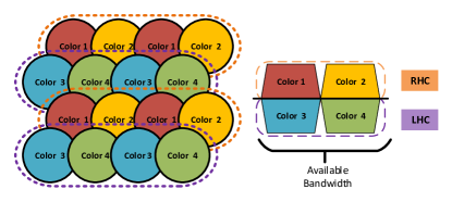
(a)

(b)

Figure 1: Examples of one-dimensional satellite coverage. (a) Four color reuse scheme. Each row of beams operate under the same polarization. (b) Two-color scheme over a coastal area. Partial Viasat-1 beam footprint [9].

For the payload, we assume that a given HPA amplifies the whole bandwidth $W^{total}$, so that the pair $j$ of two consecutive beams, with indexes $A(j)=\{2j-1,2j\},j=1,\ldots,K/2$, is served by the same amplifier. Colors alternate between consecutive beams to reduce co-channel interference, with no bandwidth overlapping. The available bandwidth $W^{total}$ is split into $2M$ carriers with a fixed carrier bandwidth $W^{\sim}=W^{total}/2M$. Thus, for $M_{b}$ carriers assigned to the beam $b$, the corresponding bandwidth is $M_{b}W^{\sim}$. We will work interchangeably with the continuous bandwidth $W_{b}$ and the discrete number of carriers per beam $M_{b}$, depending on the specific context. If an advanced payload with bandwidth flexibility is assumed, the bandwidth can be split unevenly among the beams sharing the same HPA. Alternatively, if a uniform allocation of carriers is assumed, then $M_{b}=M\;\forall\;b$. For both scenarios, and as mentioned above, co-channel interference is neglected by preventing the same carrier from being used in two adjacent beams, with $M_{a}+M_{b}\leq 2M\;\forall\;(a,b)\;\text{adjacent beams}$.

As to the carrier power, let $p_{b}^{\sim}$ be the power of the carriers that are assigned to the beam $b$. We assume an equal power allocation for all the carriers under the same HPA, so that $p_{a}^{\sim}=p_{b}^{\sim}$ for two beams $a$ and $b$ connected to the same HPA. Thus, we avoid the so-called capture effect in satellite systems with Traveling-Wave Tube Amplifiers (TWTA) when carriers with different levels are fed to a given power amplifier [8, 26]. Note that no additional impairments are assumed for the power amplification, which is considered to operate linearly. If $P_{j}^{PA}$ denotes the output power of the amplifier $j$ that serves the beams $a$ and $b$, then the carrier power is given by

$$p_{a}^{\sim}=p_{b}^{\sim}=\frac{P_{j}^{PA}}{M_{a}+M_{b}},$$ (1)

and one has that the power assigned to the beam $b$ is

$$P_{b}=p_{b}^{\sim}M_{b}.$$ (2)

The use of Multi-Port Amplifiers (MPA) furnishes the payload with a flexible allocation of the power, which can be shared by the different HPAs under the same MPA. For simplicity, we will consider an overall power budget of $P^{total}$, and a maximum power cap per HPA $P^{max}$ such that $P_{j}^{PA}\leq P^{max}\;\forall\;j$, although additional power constraints per different groups of HPAs could be considered. Alternatively, if a rigid power allocation is enforced, then all carriers are uniformly sent from the satellite with the same power as

$$p_{uni}^{\sim}=\frac{P^{total}}{KM}.$$ (3)

For the characterization of the radiation pattern, we resort to the Bessel function model [27], which facilitates the reproducibility of this study. Under this radiation pattern model, the channel gain from the $b$-th beam towards an $n$-th user within the central beam can be expressed as

$$g_{b}(n)=G_{max}\left(\frac{J_{1}(u)}{2\cdot u}+36\cdot\frac{J_{3}(u)}{u^{3}}\right)^{2},$$ (4)

with $u\approx 2.07123\cdot d_{b}(n)/R$, and $d_{b}(n)$ the distance between the $b$-th beam boresigth and the $n$-th user location. Under this model, the end-to-end channel response (including the antenna gain) of the $n$th user with respect to beam $b\in\{1,\ldots,K\}$ is denoted as $h_{b}(n)$, and the channel magnitude is obtained as

$$|h_{b}(n)|=\frac{\sqrt{G_{R}g_{b}(n)}}{\sqrt{k_{\text{B}}TW^{\sim}}4\pi D/\lambda}$$ (5)

where $G_{R}$ refers to the receive antenna gain, $\lambda$ is the carrier wavelength, and $k_{\text{B}}$, $T$ denote the Boltzmann constant and the clear sky noise temperature, respectively. Finally, the placement of the beams in the row layout is such that a distance $2R$ separates adjacent beams, for a beam radius $R$ in the Bessel model.

Parameter	Description
$K$	Number of beams
${\mathcal{N}}(b)$	Set of users on the footprint of beam $b$
${\mathcal{S}}(b)$	Set of selected users to be served by the beam $b$
$N$	Total number of users requesting traffic
$\omega_{c,n}$	Time fraction of carrier $c$ allocated to the user $n$ in the beam $b$, $n\in{\mathcal{S}}(b)$
Ω_b	Vector that collects the carrier filling at beam $b$
Ω	Vector that collects the overall carrier filling
$u_{c,n}$	Binary variable that denotes if the user $n$ is active in the carrier $c$ of the beam $b$, $n\in{\mathcal{S}}(b)$
$\bm{U}_{b}$	Vector that collects the carrier assignment for beam $b$
$\bm{U}$	Vector that collects the overall carrier assignment
$W^{total}$	Total bandwidth
$W_{b}$	Bandwidth allocated to the beam $b$
$\bm{W}$	Vector that collects the beam bandwidth allocation
$M_{b}$	Number of carriers allocated to beam $b$
$W^{\sim}$	Carrier bandwidth
$P_{b}^{\sim}$	Power per carrier at beam $b$
$P_{b}$	Power allocated to beam $b$
$P_{j}^{PA}$	Power allocated to the $j$th HPA
$P^{max}$	Maximum power per HPA
$P^{total}$	Total power
$\bm{P}$	Vector that collects the beams power allocation
$h_{b}(n)$	End-to-end channel of user $n$ with respect to beam $b$
$R^{req}(n)$	Requested rate by the $n$th user
$R^{off}(n)$	Offered rate to the $n$th user
$\zeta_{max}$	Maximum number of carriers that can be processed simultaneously by the receivers
$\mathsf{w}_{n,b}$	Bandwidth portion allocated to the $n$th user by beam $b$
$p_{n,b}$	Power portion allocated to the $n$th user by beam $b$

TABLE I: Notation summary.

III Resource Assignment

The purpose of the system under study is to match the offered rates $R^{off}(n)$ to the user demanded rates $R^{req}(n)$. This approach, which is commonly found in the literature under different constraints and variants, see, e.g., [8, 14, 3, 7, 28], will be elaborated for the different configurations under a common framework, with the aim of developing simple optimization problems.

III-A Optimization criteria

As driving metric for the allocation of resources, we use the quadratic unmet demand, since it offers a good balance between the satisfaction of the requested demand and user fairness [3, 7]. The quadratic unmet objective function reads as

$$\sum_{n=1}^{N}(R^{req}(n)-R^{off}(n))^{2},$$ (6)

that, for minimization purposes, can be alternatively expressed, by leaving out the fixed requested traffic term $R^{req}(n)$, as

$$\mathcal{U}=\sum_{n=1}^{N}(R^{off}(n))^{2}-2\sum_{n=1}^{N}R^{req}(n)R^{off}(n).$$ (7)

III-B Problem Formulation

Initially, we consider a fully flexible architecture, or equivalently, the least restrictive approach, with a satellite payload that can optimize the power and bandwidth allocated to the different users. In addition, the gateway has the capability of freely managing the beam-user mapping, so that users are not necessarily served by their dominant beams. As it is sketched in Fig 2, the flexible mapping allows for the potential pairing of a user with a non-dominant beam, such that the radiation intensity is still significant, which precludes all beams except the adjacent one for typical directive radiation diagrams.

The offered rate to the users served by beam $b$ can be expressed as

$$R^{off}(n)=\sum_{c=1}^{M_{b}}\omega_{c,n}W^{\sim}\log_{2}\left(1+\frac{p_{b}^{\sim}|h_{b}(n)|^{2}}{N_{o}W^{\sim}}\right),\,n\in{\mathcal{S}}(b)$$ (8)

where $\omega_{c,n}$ parameterizes the fraction of time that user $n$ uses the baseband frame of carrier $c$ of the beam $b$. Furthermore, with the variable $u_{c,n}$ denoting if the user $n$ is active in the carrier $c$ of the beam $b$, a carrier aggregation constraint [29] can be set as

$$\sum_{c=1}^{M_{b}}u_{c,n}\leq\zeta_{max}\;,\forall\,n\in{\mathcal{S}}(b)$$ (9)

where $\zeta_{max}$ is the maximum number of carriers that can be processed simultaneously by the receivers. In this paper, conventional user terminals are assumed, so that $\zeta_{max}=1$ for the single-carrier operation of the receive terminals.

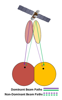
Figure 2: Different communication paths for flexible beam-user mapping.

Under this initial and most flexible approach, the user demand can be matched through the allocation of bandwidth (in continuous or discrete form, $W_{b}$ or $M_{b}$, respectively) and power $P_{b}$ to the different beams, complemented by a non-rigid mapping between users and beams. Let $\bm{P}=[P_{1},\ldots,P_{K}]\in\mathbb{R}^{K}$ and $\bm{W}=[W_{1},\ldots,W_{K}]\in\mathbb{R}^{K}$ be the vectors that collect the power and bandwidth assignment per beam, respectively. The vectors $\bm{\Omega}_{b}=[\omega_{1,1},\ldots,\omega_{M_{b},1},\,\omega_{1,2},\ldots,\omega_{M_{b},|{\mathcal{S}}(b)|}]\in\mathbb{R}^{M_{b}\cdot|{\mathcal{S}}(b)|}$ and $\bm{U}_{b}=[u_{1,1},\ldots,u_{M_{b},1},\,u_{1,2},\ldots,u_{M_{b},|{\mathcal{S}}(b)|}]\in\mathbb{R}^{M_{b}\cdot|{\mathcal{S}}(b)|}$, collect the carrier allocation and assignment for beam $b$ in (8) and (9), respectively, which are grouped in $\bm{\Omega}=[\bm{\Omega}_{1},\ldots,\bm{\Omega}_{K}]$ and $\bm{U}=[\bm{U}_{1},\ldots,\bm{U}_{K}]$, both vectors of dimension $\sum_{b=1}^{K}M_{b}|{\mathcal{S}}(b)|$.

In order to determine the bandwidth, power and mapping settings, the minimization of the unmet demand is formulated, jointly embracing the power and bandwidth allocation across the beams, the beam-user mapping, and the user-carrier mapping within each beam:

$$\begin{array}[]{ll}\displaystyle\min_{\bm{W},\bm{P},\bm{\Omega},\bm{U},{\mathcal{S}}(b)}&\mathcal{U}\\ \mbox{subject to}&\\ \hphantom{\mbox{subject to}}\text{C1:}&\sum^{K/2}_{j=1}P_{j}^{PA}\leq P^{total}\\ \hphantom{\mbox{subject to}}\text{C2:}&\sum_{b\in A(j)}P_{b}\leq P^{max},\;j=1,\ldots,K/2\\ \hphantom{\mbox{subject to}}\text{C3:}&W_{b}+W_{b+1}\leq W^{total}\quad\forall\;b\\ \hphantom{\mbox{subject to}}&M_{b}=\left\lfloor\frac{W_{b}}{W^{\sim}}\right\rfloor\;\forall\;b\\ \hphantom{\mbox{subject to}}&0\preceq\bm{W}\preceq W^{total}\\ \hphantom{\mbox{subject to}}&\sum_{n\in{\mathcal{S}}(b)}\omega_{c,n}\leq 1\;\forall\;b,\;c=1,\ldots,M_{b}\\ \hphantom{\mbox{subject to}}\text{C4:}&\sum_{c=1}^{M_{b}}u_{c,n}\leq 1\;\forall\;n\in{\mathcal{S}}(b)\\ \hphantom{\mbox{subject to}}&u_{c,n}\geq\omega_{c,n}\\ \hphantom{\mbox{subject to}}&0\leq\omega_{c,n}\leq 1\\ \hphantom{\mbox{subject to}}&u_{c,n}\in\{0,\;1\}\;\forall\;b,c,n\in{\mathcal{S}}(b)\\ \end{array}$$ (10)

where the constraint C1 is set to satisfy the overall power constraint, C2 limits the amount of power per HPA, and C3 avoids the use of the same portion of spectrum in adjacent beams to reduce the co-channel interference. Finally, C4 constraints the terminals to operate in single carrier mode.

The formulated optimization problem is non-convex due to the interplay of discrete and continuous variables, and difficult to solve. In order to make the problem more easily tractable, we will follow a two-step approach, first across beams, prior to the resource allocation inside each beam. This strategy will be followed for the different architectures in the next sections, all subsumed by the general optimization problem in (10):

• First step (beam level): Following a selected strategy, the resources at beam level are optimized in terms of power $P_{b}$, bandwidth $W_{b}$, and/or user assignment ${\mathcal{S}}(b)$.

• Second step (intra beam): After the beam resources are allocated, the carrier power per beam $p_{b}^{\sim}$ and the discrete number of carriers per beam $M_{b}$ are obtained, with the carrier assignment performed independently for each beam. The following optimization problem solves the user-carrier assignment within the beam $b$:

  $$\begin{array}[]{ll}\displaystyle\min_{\bm{\Omega},\bm{U}}&\mathcal{U}_{b}\triangleq\displaystyle\sum_{n\in{\mathcal{S}}(b)}R^{off}(n))^{2}-\\ &\hphantom{R^{off}(n))^{2}}2R^{req}(n)R^{off}(n)\\ \mbox{subject to}&\sum_{n\in{\mathcal{S}}(b)}\omega_{c,n}\leq 1,\forall\;c=1,\ldots,M_{b}\\ \hphantom{\mbox{subject to}}&\omega_{c,n}\geq 0,\forall\;c,n\\ \hphantom{\mbox{subject to}}&\sum_{c=1}^{M_{b}}u_{c,n}\leq 1\quad\forall\;n\in{\mathcal{S}}(b)\\ \hphantom{\mbox{subject to}}&u_{c,n}\geq\omega_{c,n}\\ \hphantom{\mbox{subject to}}&u_{c,n}\in\{0,\;1\},\forall\;c,n\in{\mathcal{S}}(b).\\ \end{array}$$ (11)

  This problem is an MBQP that can be solved by conventional methods such as branch and bound and/or the outer approximation approach [30, 31].

Our main goal is the derivation of optimization problems for the different cases, which are amenable for the practical implementation of the corresponding solutions. In the following sections we address the beam level optimization for different degrees of flexibility, initially for a fixed beam-user mapping, prior to a non-rigid pairing of beams and users.

IV Beam level optimization for fixed beam-user mapping

We start by exploring solutions that allow the flexible allocation of power and/or bandwidth across beams for a conventional user assignment to their dominant beams. Under this rigid mapping, we have that ${\mathcal{S}}(b)={\mathcal{N}}(b)$, i.e., the set ${\mathcal{S}}(b)$ of users served by the beam $b$ coincides with the set of users ${\mathcal{N}}(b)$ within its cell. Now, the quadratic unmet demand in (7) can be alternatively expressed after grouping users at the different beam cells:

$$\mathcal{U}=\sum_{b=1}^{K}\sum_{n\in{\mathcal{N}}(b)}\left[R^{req}(n)R^{off}(n)-\frac{1}{2}(R^{off}(n))^{2}\right].$$ (12)

In order to decouple the optimization problem in two steps, we assume that all users are offered the same rate by beam $b$:

$$R^{off}(n)=\frac{1}{|{\mathcal{N}}(b)|}R_{beam}^{off}(b),\;\forall\;n\in{\mathcal{N}}(b)$$ (13)

for an aggregated beam rate $R_{beam}^{off}(b)$, approximated by means of an effective SNR ${\mathop{\rm snr}}_{b}$, as

$$R^{off}_{beam}(b)\approx W_{b}\log_{2}(1+x_{b}\cdot{\mathop{\rm snr}}_{b})$$ (14)

where $0\leq x_{b}\leq 1$ is the fraction of total power allocated to beam $b$ such that $P_{b}=x_{b}P^{total}$. The effective SNR ${\mathop{\rm snr}}_{b}$ collects in a unique parameter the offered rate to the users across the beam $b$ with different channel qualities. This effective SNR ${\mathop{\rm snr}}_{b}$ is defined from the following equality:

$$\log_{2}(1+x_{b}\cdot{\mathop{\rm snr}}_{b})\\ =\frac{1}{|{\mathcal{N}}(b)|}\sum_{n\in{\mathcal{N}}(b)}\log_{2}\left(1+\frac{x_{b}P^{total}|h_{b}(n)|^{2}}{N_{o}W_{b}}\right),$$ (15)

and can be approximated for moderate to high SNR values, as

$${\mathop{\rm snr}}_{b}\approx\left(\prod_{n\in{\mathcal{N}}(b)}\frac{P^{total}|h_{b}(n)|^{2}}{N_{o}W_{b}}\right)^{\frac{1}{|{\mathcal{N}}(b)|}}.$$ (16)

With this, the unmet function in (12) can be written at the beam level as

$$\mathcal{U}=\sum_{b=1}^{K}\frac{1}{|{\mathcal{N}}(b)|}R_{beam}^{req}(b)R_{beam}^{off}(b)-\frac{1}{2}\frac{1}{|{\mathcal{N}}(b)|}(R_{beam}^{off}(b))^{2}$$ (17)

where

$$R_{beam}^{req}(b) =\sum_{n\in{\mathcal{N}}(b)}R^{req}(n).$$ (18)

This metric is used in the next subsections for devising different criteria for the beam resource allocation. The presented designs are collected in Table II, where a beam level optimization (first step) is explored for power, bandwidth, and both simultaneously. It has been previously reported in the literature the limited gain from power flexibility on top of bandwidth flexibility, see, e.g., [8] or [9], which can be theoretically traced back to early results in [32]. In any case, for benchmarking purposes, we will use population based metaheuristics, in particular, a genetic algorithm, to address the joint power and bandwidth allocation problem under the power and bandwidth constraints defined in Section II.

Technique	Power per carrier	Carriers per beam	Optimization problem
Beam Power Allocation	Variable	Fixed	convex QP
Beam Bandwidth Allocation	Fixed	Variable	convex QP
Beam Power & Bandwidth Allocation	Variable	Variable	non-convex QP

TABLE II: Beam-level optimization (first step) for the fixed beam-user mapping solutions.

IV-A Flexible Beam Power Allocation

First we consider a uniform bandwidth sharing for all beams, with flexible power allocation. The two colors reuse scheme is such that $M$ carriers are available per beam, for a total of $2M$ carriers, whereas the fractions of total power per beam values $x_{b},b=1,\ldots,K$, collected in $\bm{x}$, are the optimization parameters. Following the presented two-step process, the power allocation across beams is obtained in the first step after maximizing (17):

$$\begin{array}[]{ll}\mbox{max}&g(\bm{x})=\displaystyle\sum_{b=1}^{K}\frac{1}{|{\mathcal{N}}(b)|}R_{beam}^{req}(b)R_{beam}^{off}(b)-\\ \hphantom{\mbox{max}}&\hphantom{g(\bm{P})=}\frac{1}{2}\frac{1}{|{\mathcal{N}}(b)|}(R_{beam}^{off}(b))^{2}\\ \\ \mbox{subject to}&\displaystyle\sum_{b\in A(j)}x_{b}\leq\frac{P^{max}}{P^{total}},\;j=1,\ldots,K/2\\ \hphantom{\mbox{subject to}}&\displaystyle\sum_{b=1}^{K}x_{b}\leq 1,\;j=1,\ldots,K/2\\ \end{array}$$ (19)

with

$$R_{beam}^{off}(b)=\sum_{n\in{\mathcal{N}}(b)}R^{off}(n)=\frac{W^{total}}{2}\log_{2}\left(1+x_{b}\cdot{\mathop{\rm snr}}_{b}\right).$$ (20)

Note that the effective SNR ${\mathop{\rm snr}}_{b}$ in (16) is defined for the same bandwidth $W_{b}=W^{total}/2$ across beams. This problem turns out to be convex, as proven in Appendix A.

IV-B Flexible Beam Bandwidth Allocation

For the same two colors reuse scheme as above, we explore next the flexible allocation of carriers to beams, in an effort to allocate more frequency resources to more demanded beams, while still keeping the co-channel interference at low levels. The power per carrier, uniform for all beams, was given by (3), so that only the bandwidth flexibility is exploited by allowing different numbers of carriers per beam. Note that this results in a variable beam power allocation that is proportional to the bandwidth.

The optimization problem (19) is rephrased for the bandwidth allocation per beam $\bm{W}$ as

$$\begin{array}[]{ll}\mbox{max}&g(\bm{W})=\sum_{b=1}^{K}\frac{1}{|{\mathcal{N}}(b)|}R^{req}_{beam}(b)R^{off}_{beam}(b)-\\ \hphantom{\mbox{max}}&\hphantom{g(\bm{P})=}\frac{1}{2}\frac{1}{|{\mathcal{N}}(b)|}(R^{off}_{beam}(b))^{2}\\ \\ \mbox{subject to}&W_{a}+W_{b}\leq W^{total},\forall\;(a,b)\;\text{adjacent beams}.\\ \end{array}$$ (21)

With the power per beam proportional to the corresponding allocated bandwidth, the offered rate at beam $b$ is expressed as

$$R^{off}_{beam}(b)=W_{b}\log_{2}\left(1+\frac{1}{K}{\mathop{\rm snr}}_{b}\right)$$ (22)

with ${\mathop{\rm snr}}_{b}$ in (16). With this, (21) turns out to be a convex problem which provides the bandwidth allocation vector $\bm{W}$.

The allocated bandwidth $W_{b}$ needs to be formulated as a discrete number $M_{b}$ for the intra-beam carrier-user mapping. Thus, the number of carriers per beam is obtained as

$$M_{b}=\frac{W_{b}}{W^{total}/2}M.$$ (23)

As computed, $M_{b}$ will not be in general integer, so that it must be rounded in such a way that the same carrier is not used in adjacent beams.

IV-C Flexible Power and Bandwidth Allocation

For benchmarking purposes it is desirable to evaluate the performance of a potential scheme able to allocate both bandwidth and power across beams, together with the intra-beam sharing of resources. This general problem, as stated in (10), is a hard one, as described, for example, in [9]. Therein, a genetic algorithm is used, motivated by encouraging results in previous works such as [28]. The details of the genetic algorithm which have been implemented for this work can be found in Appendix B.

V Beam level optimization for flexible beam-user mapping

In the previous section, power and/or bandwidth were flexibly allocated to the different beams for a fixed assignment between users and beams. Conventionally, users are served by their dominant beams, even though the additional freedom provided by a flexible mapping between users and beams can be exploited to balance the beam load, as illustrated in previous works dealing with the hot-spot scenario [19], [20], [21]. As in the previous first level designs, the goal is to pose a convex problem for the practical implementation of the resource allocation at beam level. Thereby, the framework for the beam level optimization derived from (12) needs to be modified to accommodate a non-rigid allocation of users to beams.

A flexible power allocation does not lead easily to a tractable problem in combination with the optimization of the beam-user mapping. In addition, the power flexibility was seen to provide limited gain, at least with respect to the corresponding bandwidth allocation across beams [8]. Therefore, beam-user mapping will be considered to enhance only flexible bandwidth solutions. The allocation of carriers to beams will be relaxed, so that continuous variables will be considered when assigning spectral resources to beams. All in all, the simplifications that we will apply on the general optimization problem (10) are listed as:

1. The variables denoting the bandwidth allocated to the different beams will be continuous, thus relaxing the discrete nature of carriers. At the end rounding is applied to obtain an integer number of carriers per beam.

2. The power per carrier is not a free parameter, but rather a fixed predefined value, in such a way that those beams with fewer allocated carriers will consume less power.

For benchmarking purposes, a design with fixed bandwidth allocation and flexible mapping is also assumed. These designs are collected in Table III and presented in the following subsections.

Technique	Power per carrier	Carriers per beam	Optimization problem
Beam-user Mapping	Fixed	Fixed	Convex QP
Beam-user Mapping & Flexible Bandwidth Allocation	Fixed	Variable	Convex QP

TABLE III: Beam-level optimization (first step) for the flexible beam-user mapping solutions.

V-A Joint optimization of bandwidth and beam-user mapping

By following the relaxation described above, we can alternatively express the optimization problem (10) as the following convex Quadratic Programming (QP) problem:

$$\begin{array}[]{ll}\displaystyle\min_{\bm{\mathsf{w}}}&\mathcal{U}\\ \mbox{subject to}&R^{off}(n)=\displaystyle\sum_{b=1}^{K}\mathsf{w}_{n,b}\log_{2}\left(1+\frac{p_{n,b}|h_{b}(n)|^{2}}{N_{o}\mathsf{w}_{n,b}}\right)\\ \hphantom{\mbox{subject to}}&\displaystyle W_{b}=\sum_{n=1}^{N}\mathsf{w}_{n,b}\\ \hphantom{\mbox{subject}}\text{C1:}&W_{b}+W_{b+1}\leq W^{total}\quad\forall b\\ \hphantom{\mbox{subject}}\text{C2:}&\sum_{b=1}^{K}\mathsf{w}_{n,b}\leq W^{\sim}\quad\forall n\\ \hphantom{\mbox{subject to}}&\mathsf{w}_{n,b}\geq 0\end{array}$$ (24)

where $\bm{\mathsf{w}}=[\mathsf{w}_{1,1},\ldots,\mathsf{w}_{N,1},\,\mathsf{w}_{1,2},\ldots,\mathsf{w}_{N,K}]\in\mathbb{R}^{N\cdot K}$, and $\mathsf{w}_{n,b}$ and $p_{n,b}$ are the portions of the bandwidth and power, respectively, allocated to the $n$th user by beam $b$; note that the power is proportional to the bandwidth as $p_{n,b}=\mathsf{w}_{n,b}\frac{P^{total}}{K}\frac{2}{W^{total}}$. Constraint C1 ensures that the bandwidth is not reused in consecutive beams, whereas constraint C2 limits the bandwidth that can be allocated to a given user to that of a carrier.

Once the relaxed problem is solved, the bandwidth of the beam $b$ is obtained as $W_{b}=\sum_{n=1}^{N}\mathsf{w}_{n,b}$, and the procedure detailed in Section IV-B can be followed to obtain the number of carriers per beam $M_{b}$. The beam-user mapping is also extracted from $\mathsf{w}_{n,b}$, with the user $n$ assigned to the beam offering the maximum bandwidth as $\arg\max_{b}\mathsf{w}_{n,b}$. Note that some users could remain unpaired after the beam-level optimization, for example if they demand low relative rates in highly asymmetric traffic settings. Nevertheless, we want to ensure the mapping of every user in the first step and leave the decision of the resource assignment to the subsequent intra-beam processing in the second step. To this end, we assume that every user is assigned to its dominant beam unless the optimization says otherwise.

V-B Beam-user mapping with fixed bandwidth

If the bandwidth allocation is fixed, the constraint C1 in (24) needs to be reformulated, since the set of available carriers per beam is fixed, and such that $W_{b}\leq M\cdot W^{\sim}$. The outcome of the optimization problem will be the beam-user assignment; this solution can be applied to conventional payloads with fixed allocation of resources, since the radio resource management is the only unit required to enforce this additional flexibility. Other system implications are discussed in the next section.

VI System requirements for flexible beam-user mapping

In conventional satellite systems, a rigid beam-mapping is assumed, for which users need to report a single magnitude value to quantify the quality of the link with their respective dominant beam. If flexible beam-user mapping is applied, then the gateway can serve a given user through a non-dominant beam if required. This flexibility can be exploited if the gateway knows the corresponding channel magnitude; thus, user terminals need to report back the magnitude of their two downlink strongest channels. Note that, under this paradigm, a given user will be served only by its dominant beam or the strongest adjacent beam; in other words, flexible mapping with non-dominant beam assignment can be enforced if the alternative beam radiates a minimum power at the intended location.

From the above, the implementation at the system level of the flexible user-mapping requires the knowledge of two channel quality magnitude values per user. Since consecutive beams operate in alternate frequency bands, and the simultaneous channel estimations cannot be pursued with standard single-carrier user terminals, some system add-ons are needed, which can be based on existing solutions. The first solution can be based on the handover mechanisms in the standardized mobile satellite system [33], where a common frequency can be reused in every beam for the simultaneous channel estimation with the application of unique spreading sequences for each beam. It should be remarked that this common frequency is only employed for the system synchronization and management of the user terminals; conventional orthogonal carriers are employed for on-demand data channels. Alternatively, a user position method can be also devised similarly to the handover management in DVB-S2 [34, 35]. In that case, user terminals report its location along with the channel estimation of its dominant channel, and the gateway could infer the channel strength of the adjacent beams if a accurate model of the radiation pattern is available. In any case, note that a handover operation can be enforced even for a static user, as it is a system level decision accounting for global metrics. Finally, let us remark that the proposed flexible beam-user mapping is fully compatible with the existing air interface standards, such as DVB-S2X, even avoiding the use of the new features of DVB-S2X supporting intermittent transmissions as needed for beam hopping, and with a low demand for the channel state information in the feedback channel, as compared to precoding schemes.

VII Performance evaluation

Technique	Label	Carrier Power	Carrier Bandwidth	Number of carriers per beam	User mapping	Optimization
Beam Power Allocation	POW	Variable	Fixed	Fixed	Dominant beam	Two step: (i) Convex (ii) MBQP
Beam Bandwidth Allocation	BW	Fixed	Fixed	Variable	Dominant beam	Two step: (i) Convex (ii) MBQP
Beam Power&Bandwidth Allocation (Benchmark)	BW-POW	Variable	Variable	Variable	Dominant beam	Two step: (i) Genetic Algorithm (ii) MBQP
Beam-user Mapping with fixed resources per beam	MAP	Fixed	Fixed	Fixed	Free assignment	Two step: (i) Convex (ii) MBQP
Beam-user Mapping with flexible Bandwidth per Beam	BW-MAP	Fixed	Fixed	Variable	Free assignment	Two step: (i) Convex (ii) MBQP

TABLE IV: Summary of the considered techniques.

In this section, we evaluate the performance of the proposed design with flexible beam-user mapping for different payload architectures. A comprehensive summary of the explored techniques is presented in Table IV. These techniques will be applied to the model in Section II with the parameters in Table V. The solutions of the corresponding optimization problems are obtained with two tools, namely, the Mosek solver [36] and the optimization toolbox CVX [37], for the mixed integer and the convex problems, respectively. As detailed later, the traffic demand density per beam will follow different traffic profiles across beams; 500 Monte-Carlo realizations will be run to account for random traffic variations. Note that, as per Table V, only six beams will be considered to keep the complexity of the simulations relatively low. Nevertheless, the analyzed methods operate with an arbitrary number of beams, and numerical results not shown here reveal that conclusions hold for larger scale scenarios.

Diagram pattern	Bessel modeling
Number of beams	6
Maximum antenna gain	52 dBi
Average free space losses	210 dB
Average atmospheric losses	0.4 dB
Total available transmission power, $P^{total}$	200 W
Maximum power per HPA, $P^{max}$	133 W
Total available bandwidth, $W$	500 MHz
Polarization	Single
Frequency reuse scheme	2-Color
Number of carriers per color, $M$	4
Frequency band [GHz]	20
Receiver Parameters
Terminal G/T	16.25 dB/K
Losses due to terminal depointing	0.5 dB

TABLE V: System parameters for the forward link.

VII-A Considerations on the co-channel interference

Following the described model in Section II, with a two-color pattern, the co-channel interference can be neglected, as justified next. For a uniform power and bandwidth allocation, the assumption holds when users are served by their dominant beam. This can been seen clearly in Fig. 3, where the signal-to-noise ratio (SNR) and signal-to-interference-and-noise ratio (SINR) are displayed for different user locations within a given cell. Note that the uniform allocation of frequency carriers, with a given carrier used every two beams, is the worst case in terms of co-channel interference, since the uneven distribution of bandwidth across beams can place interfering carriers in more distant beams. Quite the opposite, the peripheral areas of the cells can suffer from higher interference if power can be flexibly allocated, and skewed power beam distributions are applied as a result. In consequence, those solutions based on a flexible allocation of power can yield slightly optimistic results. Furthermore, the co-channel interference can limit the allocation of resources from neighbour beams, as displayed in Fig. 4. In order to keep the practical assumption on the interference, an SINR threshold is enforced and the resource pulling from neighbour beams is constrained to operate in the inward blue area displayed in Fig. 5; this ensures a minimum carrier to interference (C/I) of $23$ dB with no significant impact on the SINR. For reference, the SNR at the center of the beam is approximately $15$ dB with the satellite parameters in Table V, which goes down to $8.7$ dB when users are served by a non-dominant beam . As additional information, the resource pulling area amounts to around $12\%$ of the overall beam area.

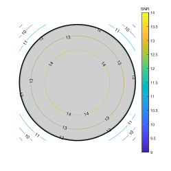
(a)

(b)

Figure 3: Contour map of the signal strength within a beam for uniform resource allocation. The grey area displays the beam footprint at 3 dB. (a) SNR, (b) SINR.

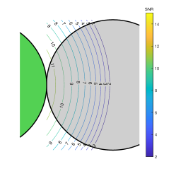
(a)

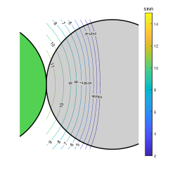
(b)

Figure 4: Contour map of the signal quality when users are served by a non-dominant beam (green beam). The grey area displays the beam footprint at 3 dB: (a) SNR, (b) SINR.

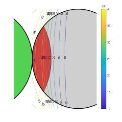
Figure 5: Contour map of the carrier to interference (C/I) ratio when users are served by a non-dominant beam (green beam). The grey area displays the beam footprint at 3 dB. The inward red area hosts those users that can be served by a non-dominant beam.

VII-B Traffic Model

For reference purposes we will consider the satellite capacity, interpreted as the total average throughput that the satellite can deliver when resources (power and bandwidth) are uniformly allocated across beams. For the case under study, the capacity of the system is $T=6.8$ Gbps for the six considered beams. This value is obtained by concentrating all the demand at each cell in a single user with SNR = 13.5 dB, which is the effective SNR for the system parameters in Table V and users uniformly distributed within the beam footprint.

We assume that every user demands a rate of $25$ Mbps; in an attempt to use up the overall capacity $T$, we try to accommodate 272 users across the different beams. We employ the Dirichlet distribution $Dir(K,\alpha)$, with $\bm{\alpha}=[\alpha_{1},\dots,\alpha_{K}]$, to model the different traffic profiles while ensuring that the overall capacity $T$ is requested; the $\alpha_{i}$ parameters feature the possible statistically different traffic demands across cells. In particular, we portray three different scenarios in this work:

1. Homogeneous traffic (HT): A homogeneous exploration of the different traffic distributions is made with equal probability for every possible distribution of users among cells. This setting is modelled with $\alpha_{i}=1,\;i=1,\dots,K$.

2. Hot-Spot (HS): A high amount of traffic is requested by users in one cell, with adjacent colder cells, in what is known as the HS scenario [19, 20, 21]. This non-uniform setting is modelled with $\bm{\alpha}=[5\;5\;30\;5\;5\;5]$, where the cell with index 3 is selected as the HS.

3. Wide Hot-Spot (WHS): Another asymmetric scenario is explored, with two highly congested cells surrounded by colder cells. In this case, we place the high traffic demand in the footprints of beams sharing the same HPA. Following the notation involving the HPAs in Section II, this setting is modeled with $\bm{\alpha}=[10\;10\;40\;40\;10\;10]$ by placing the congestion in the cells with indexes 3 and 4..

The number of users per cell is obtained as follows. First, $K$ random numbers are taken from the Dirichlet distribution $Dir(K,\alpha)$. Then, they are multiplied by 272 and rounded accordingly. Next, users are uniformly distributed across the geographical locations of each cell. The traffic demand per cell, i.e., the number of users multiplied by $25$ Mbps, will be characterized by its standard deviation, ranging from 0 (uniform traffic demand) till $\sqrt{K-1}\frac{T}{K}$ (all traffic requested from a single beam). For illustration purposes, the empirical probability distribution function of the standard deviation of the cells traffic demand are presented in Fig. 6 for the explored scenarios.

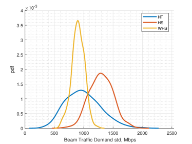
Figure 6: Empirical probability distribution function of the standard deviation of the cells traffic demand, 500 realizations.

VII-C Numerical Results

Technique	Label	NQU	NU	Offered Rates [Gbps]	Minimum Rate [Mbps]
Beam Power Allocation	POW	0.162	0.337	4.511	10.41
Beam Bandwidth Allocation	BW	0.134	0.269	4.979	6.59
Beam Power&Bandwidth Allocation (Benchmark)	BW-POW	0.088	0.218	5.323	9.41
Beam-user Mapping with fixed resources per beam	MAP	0.113	0.248	5.116	11.72
Beam-user Mapping with flexible Bandwidth per Beam	BW-MAP	0.084	0.219	5.312	12.63

TABLE VI: Average performance of the techniques in the HT scenario. The capacity of the satellite is $T=6.8$ Gbps, which is the aggregated rate requested by the users.

As seen above, the quadratic unmet capacity in (7) is the baseline metric for optimization purposes. However, for a better understanding of the demand supply and comparison purposes, the following normalized parameters will be used:

1. Normalized quadratic unmet capacity:

   NQU $$=\frac{\displaystyle\sum_{n=1}^{N}(R^{req}(n)-R^{off}(n))^{2}}{N\left(W^{\sim}{\log_{2}(1+\mathop{\rm snr}_{eff})}\right)^{2}}$$ (25)

   with $\mathop{\rm snr}_{eff}$ an effective SNR corresponding to a super-user that embodies the user channels across all locations, such that

   $$\log_{2}(1+{\mathop{\rm snr}}_{eff})=\mathbb{E}_{h}\left[\log_{2}\left(1+\frac{P_{uni}^{\sim}|h|^{2}}{N_{o}W^{\sim}}\right)\right]$$ (26)

   where $h$ is a random channel value, and the expectation is taken across all locations within the beam. Under this normalization, values close to 0 correspond to a better resource flexibility to provide the requested traffic, whereas higher values indicate the opposite.

2. Normalized unmet capacity:

   $$\text{NU}=\displaystyle\frac{T-\sum_{n=1}^{N}R^{off}(n)}{T}$$ (27)

   with $T$ the satellite capacity. This is a common metric found in the literature [7, 8, 9, 25]. Note that for our simulations we are assuming that the aggregated rate of all users is equal to $T$, i.e.,

   $$T=\sum_{n=1}^{N}R^{req}(n)$$ (28)

   since we are interested in studying the impact of the different load across beams.

In addition, the minimum rate for each simulated scenario will be also detailed to asses the fairness of the corresponding rate allocation scheme.

As initial assessment of the different degrees of flexibility in the resource assignment, we address the HT scenario. The average performance of the different system metrics is collected in Table VI, where the normalized parameters NQU and NU are listed along with the averaged offered and minimum rates.

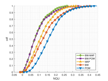
Figure 7: Cumulative distribution function of the normalized quadratic unmet capacity in the HT scenario.

A first relevant observation is that the adjustability when mapping beams and users, or allocating power, enhances similarly the performance of bandwidth flexibility. This can be seen clearly in Fig. 7, that displays the Cumulative Distribution Function (CDF) of the normalized quadratic unmet capacity. Note, however, that the implications of both schemes are different; on the one side, an ideal scenario is considered for the flexible power allocation and more practical constraints should be enforced for the power amplification [8]: a change in the operation point of a power amplifier modifies its power efficiency and the intermodulation interference caused by the non-linearity. On the other side, the complexity of the associated optimization is significantly different, with a genetic algorithm used to solve the joint power and bandwidth allocation problem. In this regard, some attempts can be found in the literature to conceive a convex optimization problem as an approximation, see, e.g. [7, 10].

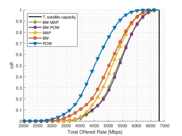
Figure 8: Cumulative distribution function of the total offered rate in the HT scenario.

Remarkably, we can also see from Fig. 7 that under a fixed allocation of the payload resources to the different beams, the flexible beam-user mapping by itself can provide a competitive performance against the conventional rigid mapping with adjustable beam bandwidth. In addition, let us note that the lack of competitiveness of power flexible solutions agrees with previous results in the literature [8, 9].

In terms of the offered rates, previous conclusions hold, with similar performance of both beam-user mapping and flexible power allocation when pairing together with a flexible allocation of bandwidth, enhancing the performance of the latter around 6%, as concluded from Table VI. A detailed view is presented in Fig. 8, where the CDF of the total offered rates for the different techniques is displayed.

Fairness in the provision of rates is also relevant; in particular, the average minimum rate for all users is displayed in Table VI, with the corresponding CDF in Fig. 9. We can see that the flexible bandwidth combines better, from a fairness perspective, with the smart beam-user mapping rather than the adjustable power allocation, achieving higher probabilities for intermediate minimum rates.

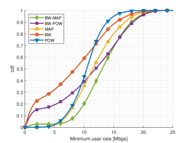
Figure 9: Cumulative distribution function of the minimum rates in the HT scenario.

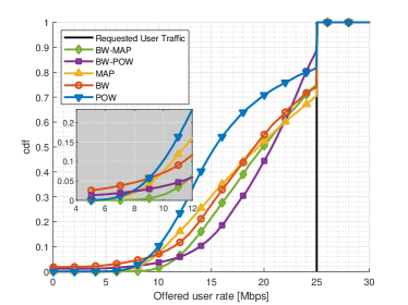
Figure 10: Cumulative distribution function of the offered user rates in the HT scenario.

In addition, the CDF of all user rates across the explored traffic demand distribution is presented in Fig. 10. Despite the similar performance in terms of the average quadratic unmet capacity in Table VI, both flexible power allocation and smart mapping of the users pursue the provision of the user demand differently when paired together with the flexible bandwidth. By inspecting Fig. 10, the former exchanges both lower and higher ends of the user rates for more users with intermediate rates, as compared with the latter. The flexible beam user-mapping raises the floor with a 9% of improvement on the average minimum rate in Table VI, whereas granting full rate to more users, in particular 13% higher by looking at the cross of both curves with the requested user traffic abscissa in Fig. 10. Finally, note in the same figure that the flexible beam-user mapping enhances notably the performance of flexible bandwidth when combined, as early hinted in [23].

Case	Technique	Label	NQU	NU	Offered Rates [Gbps]	Minimum Rate [Mbps]
HS	Rigid mapping	BW	0.253	0.388	4.164	0.88
	Power Flexibility	BW-POW	0.189	0.321	4.624	2.47
	Beam-user Mapping	BW-MAP	0.126	0.284	4.874	10.72
WHS	Rigid Mapping	BW	0.172	0.336	4.515	9.5
	Power Flexibility	BW-POW	0.110	0.278	4.913	12.70
	Beam-user Mapping	BW-MAP	0.112	0.256	5.059	12.13

TABLE VII: Average performance of the explored techniques in the Wide Hot-Spot (WHS) and Hot-Spot (HS) scenarios.

So far, we have addressed diverse traffic profiles in the HT scenario without favouring any particular placement of the traffic among cells. However, the flexible beam-user mapping can particularly excel under strongly skewed traffic distributions. To this end, the techniques under comparison are also tested in two different asymmetric scenarios. First, we address an especially skewed case, the Hot-Spot (HS) scenario, with one congested beam, surrounded by colder beams; the corresponding numerical results are collected in Table VII. For the sake of clarity, we discard those schemes with fixed bandwidth allocation, and label the techniques in terms of their additional flexibility on top of the flexible bandwidth allocation hereafter. For illustration purposes, an example of user distribution is sketched in Fig. 11a, with the average requested and offered traffic per beam presented in Fig. 11b. Note that, in this HS case, both rigid and flexible mapping solutions devote most of the resources to the congested beam, depriving almost completely the two colder adjacent beams of any offered throughput. By just allowing an alternative link, the flexible beam-user mapping can trade off some offered traffic in the congested beam for a better match of the traffic demand in the colder beams, with an improvement on the data provision around 5% and 17%, on average, over the adjustable power allocation and rigid mapping, respectively. Remarkably, this improvement is obtained in a cooperative way, as it can be observed from the example in Fig. 11a, and the smart beam-user mapping results in a joint effort to supply the traffic demand with multiple beams involved in the resource pulling, some of them far away from the concentration of high traffic demand. As a matter of fact, the flexible association between users and beams leads to better matching of the traffic demand with a reduction on the average quadratic unmet demand around 33% and 50% against the power flexibility and rigid mapping, with substantial improvements on the minimum rates in both cases. The improvement with the flexible-beam user mapping is evident from the CDF curves of the normalized quadratic unmet capacity, total offered rates, minimum user rates and offered user rates in Fig. 12, 13, 14 and 15, respectively. It is highly remarkable the improvement on the minimum rate for the HS scenario provided by the BW-MAP scheme, as per Table VII and Fig. 14. This comes from a more fair allocation or resources to those beams adjacent to the congested one, which in turn receives a slightly lower rate as compared to other schemes (see Fig. 11).

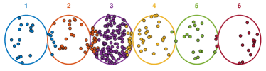
(a) User location for a given realization. The circles represents different user locations, and are filled with a color denoting the beam which serves the corresponding user in the case of flexible beam-user mapping combined with flexible bandwidth.

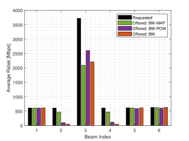
(b) Average requested and offered traffic per beam.

Figure 11: Hot-Spot scenario.

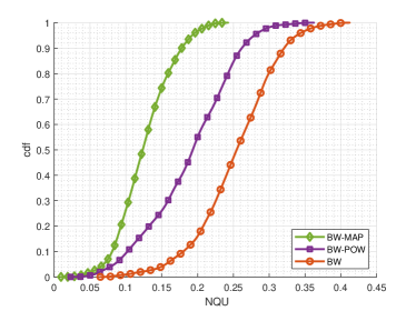
Figure 12: Cumulative distribution function of the normalized quadratic unmet capacity in the Hot-Spot (HS) scenario.

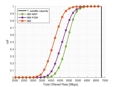
Figure 13: Cumulative distribution function of the total offered rate in the Hot-Spot (HS) scenario.

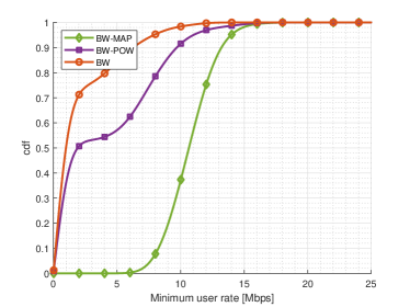
Figure 14: Cumulative distribution function of the minimum rates in the Hot-Spot (HS) scenario.

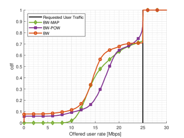
Figure 15: Cumulative distribution function of the offered user rates in the Hot-Spot (HS) scenario.

Finally, we consider the WHS scenario, with two strongly congested beams surrounded by colder beams, as sketched in Fig. 16a for a given realization. The average requested and offered rates per beam are depicted in Fig. 16b, with performance metrics detailed in Table VII. From this table, the flexible beam-user mapping provides a reduction of around 35% in terms of quadratic unmet demand against the rigid beam-user mapping in the WHS scenario; the improvement is clear from the CDF of the normalized quadratic unmet demand in Fig. 17. This results in both better demand satisfaction and fairness in the system. The smart mapping of the users increases the demand satisfaction, close to 12%, and also raises the floor of the user rates with increments of the minimum user rate of approximately 28% against the rigid mapping. This better performance can be seen in Figs. 18, 19 and 20, which display the CDF of the total offered rates, minimum user rates and offered user rates, respectively. Note that the overlapping bandwidth constraint limits the number of carriers available for the users in congested cells in caes of rigid mapping. Interestingly, the flexible beam-user mapping overcomes these limitations through a smart association of users and beams, and performing a cooperative provision of the user rates. On the other hand, the adjustable power allocation presents a close performance to the flexible beam-user mapping in terms of quadratic unmet demand as reflected in Fig. 17. However, we should be keep in mind that the performance with adjustable power allocation is somewhat optimistic, so that enforcing more realistic power constraints would yield an additional edge for the flexible beam-user mapping solution.

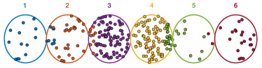
(a) User location for a given realization. The circles represents different user locations, and are filled with a color denoting the beam which serves the corresponding user in the case of flexible beam-user mapping combined with flexible bandwidth.

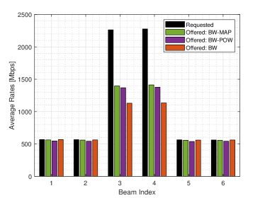
(b) Average requested and offered traffic per beam

Figure 16: Wide Hot-Spot scenario.

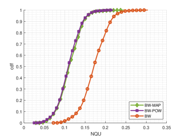
Figure 17: Cumulative distribution function of the normalized quadratic unmet capacity in the Wide Hot-Spot (WHS) scenarios.

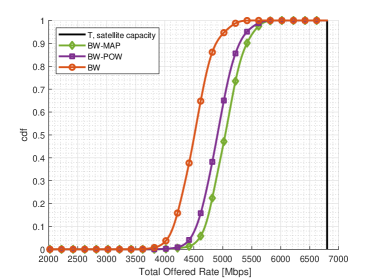
Figure 18: Cumulative distribution function of the total offered rate in the Wide Hot-Spot (WHS) scenarios.

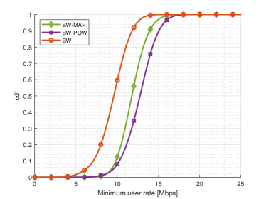
Figure 19: Cumulative distribution function of the minimum rates in the Wide Hot-Spot (WHS) scenarios.

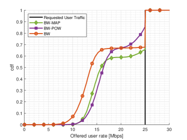
Figure 20: Cumulative distribution function of the offered user rates in the Wide Hot-Spot (WHS) scenarios.

As a final remark, let us note that the performance evaluation in this section was obtained for a fixed satellite antenna radiation diagram, and it is left for future studies the joint optimization of both user assignment and beamforming. As an illustration, hot-spot like scenarios can benefit from a non-rigid steering of the satellite beams, as pointed out in [24]. Advanced adaptive beamforming capabilities, if available, can be employed to modulate the beams load and contribute to a smoother service, even in the absence of flexible RRM. Additionally, flexible beam-user mapping can provide load transferring capabilities without requiring the use of active antennas. Furthermore, both load managing approaches are not exclusive and can be jointly optimized. Thus, the flexible beam-user mapping could simplify the beamforming requirements for transferring the traffic load.

VIII Conclusions

This work has explored the improvement margin from a flexible pairing between users and beams, with particular emphasis on flexible payloads, for which radio resource management is instrumental to serve spatially non-uniform traffic demands in satellite multibeam footprints. Under the proposed user-centric approach, a two-step optimization process has revealed as a practical strategy, with a first convex optimization problem allocating carriers, power and/or users to the different beams. A second optimization step, operating at beam level, assigns carriers to users. The Dirichlet distribution has been chosen to feature different random traffic demands, due to its capability to shape the traffic profile across beams. From the results, it can be concluded that a non-rigid association between users and beams, operating jointly with a flexible allocation of bandwidth, can compete with a joint power-bandwidth allocation, even with ideal conditions and lenient constraints for the power allocation. This comes without noticeable additional complexity at the different subsystems, and with more simple optimization schemes. Remarkably, for those cases for which traffic is severely asymmetric across beams, in hot-spot like cases, the use of a flexible beam-user mapping can report significant benefits when serving the requested traffic levels.

Acknowledgment

Funded by the Agencia Estatal de Investigación (Spain) and the European Regional Development Fund (ERDF) through the project RODIN (PID2019-105717RB-C21). Also funded by Xunta de Galicia (Secretaria Xeral de Universidades) under a predoctoral scholarship (cofunded by the European Social Fund). The views of the authors of this paper do not necessarily reflect the views of the European Space Agency.

Appendix A Convexity proof of the beam power optimization

We can write $g(\bm{x})$ in (19) as the sum of separable functions, so that the optimization problem for the vector $\bm{x}=(x_{1},\ldots,x_{K})$ of fractions of total power per beam reads as

$$\begin{array}[]{ll}\mbox{max}&g(\bm{x})=\frac{1}{2}\left(\frac{W^{total}}{2}\right)^{2}\\ &\hphantom{g(\bm{x})=\frac{1}{2}}\cdot\sum_{b=1}^{K}\frac{1}{|\mathcal{N}(b)|}\left(f_{b}(x_{b})-g_{b}(x_{b})\right)\\ \\ \mbox{subject to}&\sum_{b\in A(j)}x_{b}\leq\frac{P^{max}}{P^{total}},\;j=1,\ldots,K/2\\ \hphantom{\mbox{subject to}}&\sum_{b=1}^{K}x_{b}\leq 1\end{array}$$ (29)

with

$$f_{b}(x) \triangleq 2S^{req}(b)\log_{2}\left(1+x\cdot{\mathop{\rm snr}}_{b}\right)$$ (30)

$$g_{b}(x) \triangleq \log_{2}^{2}\left(1+x\cdot{\mathop{\rm snr}}_{b}\right)$$ (31)

and the requested spectral efficiency $S^{req}(b)=R^{req}(b)/(W^{total}/2)$.

It can be proved that $f_{b}(x)-g_{b}(x)$ is a quasiconcave function for positive $x$; unfortunately, the sum of quasiconcave functions is not guaranteed to be quasiconcave, which would help to come up with an efficient optimization algorithm. In fact, it can be checked that the sum in (29) is not necessarily quasiconcave in all cases. Nevertheless, concavity of the function $f_{b}(x)-g_{b}(x)$ can be analyzed in detailed; its second derivative is given by

$$\frac{\partial^{2}}{\partial x^{2}}(f_{b}(x)-g_{b}(x))=\\ -\text{cst}\frac{S^{req}(b)-\log_{2}(1+x\cdot{\mathop{\rm snr}}_{b})+\log_{2}e}{(1+x\cdot{\mathop{\rm snr}}_{b})^{2}}$$ (32)

with cst a positive constant. Since the offered traffic must be lower than the requested traffic, i.e., $\log_{2}(1+x\cdot{\mathop{\rm snr}}_{b})\leq S^{req}(b)$, we have that the second derivative is negative for the range of admissible values of $x$ and, in consequence, problem (29) and, equivalently, (19), is convex.

Appendix B Genetic Algorithm implementation

In a genetic algorithm, individuals evolve from previous solutions with the aim to optimize a given objective function. This evolution process is composed of four main operations:

• Mutation: The attributes of a individual are randomly modified. When generating a new generation, there is a probability $p_{mut}$ of a individual to be affected by this mutation.

• Selection of the fittest: In each iteration, an operation is made to select the parents to generate the new individuals in the next generation.

• Crossover: The characteristics of two parents are stochastically combined to generate new individuals. This operations is applied with a probability $p_{cross}$ by selecting two random parents.

• Elite members: A determined number of the best solutions are set as new individuals for the next generation and remain unchanged.

For the genetic algorithm design, we follow a similar implementation to [9], with the bandwidth and power per beam as individuals of the algorithm. For the benchmark solution, we define $\bm{C}=[M_{1},\ldots,M_{K}]\in\mathbb{Z}^{K}$ as the vector that collects the number of carriers per beam $M_{b}$. Then, we set the pair of vectors $\bm{P}$ and $\bm{C}$ as the inputs of the algorithm. The evolution process is driven by the combinations of $\bm{P}$ and $\bm{C}$, which have to be ranked. We employ the geometric mean of the user channels under the footprint of the beam $b$ to obtain a reference channel $h_{b}^{ref}$. Then, the requested and offered traffic in the beam $b$ are computed as

$$R_{beam}^{req}(b) =\sum_{n\in{\mathcal{N}}(b)}R^{req}(n)$$ (33)

$$R^{off}_{beam}(b) =W_{b}\log_{2}\left(1+\frac{P_{b}|h_{b}^{ref}|^{2}}{N_{0}W_{b}}\right),\quad W_{b}=M_{b}W^{\sim}$$ (34)

and the quadratic unmet function is evaluated as

$$\mathcal{U}=\sum_{b=1}^{K}\left(R_{beam}^{req}(b)-R^{off}_{beam}(b)\right)^{2}.$$ (35)

For further details of the algorithm implementations, Table VIII collects the settings employed by the genetic algorithm; particular crossover and mutation functions are employed for integer inputs [38]. In addition, an in-between process is considered, as the randomly generated individuals do not always satisfy the overall power constraint and beam bandwidth overlapping constraints. To resolve this, the same approach as in [9] is made to repair the incorrect solutions to satisfy the constraints:

• Power constraints: To satisfy the sum power constraint, the vector $\bm{P}$ is scaled down by a factor $k$. If the sum power of a vector $\bm{P}$ is given by $P_{sum}$ and it is higher than $P^{total}$, then the power is scaled down by $k=\frac{P^{total}}{P_{sum}}$. In addition, the power is also modified to satisfy the HPA power constraints: $\sum_{b\in A(j)}P_{b}\leq P^{max},\;j=1,\ldots,K/2$.

• Bandwidth overlapping constraint: To avoid the overlapping frequencies between two neighbour beams, the bandwidth constraint C3 in (10) has to be satisfied. After selecting randomly an increasing or descending order of the beams, the bandwidth constraint is enforced in an iterative process that goes through all possible beam indexes $b$. If $W_{b}+W_{d}>W^{total}$ during the process, with $d=\{b-1,b+1\}$ depending on the selected order, then we set $W_{b}=W^{total}-W_{d}$ to satisfy the overlapping bandwidth constraint with $W_{b}=M_{b}W^{\sim}$. However, this process can produce an inefficient bandwidth allocation with unused portions of bandwidth (see Fig. 21). For a given triplet of beams, the unused bandwidth $W_{un}$ is expressed as

  $$W_{un}=W^{total}-W_{c}-\max(W_{l},W_{r})$$ (36)

  where $c,l,r$ are the central, left and right beam indices of the triplet. Different central beams can be chosen, so that the beams with higher traffic demand are considered first, and the corresponding unused bandwidth $W_{un}$ is assigned to them, till no residual unused bandwidth is left.

Figure 21: Example for which the available bandwidth is not fully allocated to beams 1, 2 and 3. The color of beam 2 is different from the color of beams 1 and 2 [9].

Parameter	Value
Selection operator	Tournament
Crossover operator	Laplace crossover
Mutation operator	Power mutation
Max. number of generations	5000
Population size	4000
Tournament size	5
Elite members	20
Crossover prob.	0.8
Mutation prob.	0.1

TABLE VIII: Genetic algorithm settings[38].

References

- [1] P. Angeletti and J. L. Cubillos, “Traffic balancing multibeam antennas for communication satellites,” IEEE Transactions on Antennas and Propagation, pp. 1–1, 2021.
- [2] U. Park, H. W. Kim, D. S. Oh, and B. J. Ku, “Flexible Bandwidth Allocation Scheme Based on Traffic Demands and Channel Conditions for Multi-Beam Satellite Systems,” in 2012 IEEE Vehicular Technology Conference (VTC Fall), 2012, pp. 1–5.
- [3] J. P. Choi and V. W. Chan, “Optimum power and beam allocation based on traffic demands and channel conditions over satellite downlinks,” IEEE Trans. Wireless Commun., vol. 4, no. 6, pp. 2983–2993, 2005.
- [4] T. Qi and Y. Wang, “Energy-efficient power allocation over multibeam satellite downlinks with imperfect CSI,” in 2015 International Conference on Wireless Communications Signal Processing (WCSP), 2015, pp. 1–5.
- [5] C. N. Efrem and A. D. Panagopoulos, “Dynamic Energy-Efficient Power Allocation in Multibeam Satellite Systems,” IEEE Wireless Commun. Lett., vol. 9, no. 2, pp. 228–231, 2020.
- [6] J. Lei and M. A. Vázquez-Castro, “Joint Power and Carrier Allocation for the Multibeam Satellite Downlink with Individual SINR Constraints,” in 2010 IEEE International Conference on Communications, 2010, pp. 1–5.
- [7] A. L. Heng Wang and X. Pan, “Optimization of Joint Power and Bandwidth Allocation in Multi-Spot-Beam Satellite Communication Systems,” Math. Probl. Eng., vol. 214, 2014.
- [8] G. Cocco, T. De Cola, M. Angelone, Z. Katona, and S. Erl, “Radio Resource Management Optimization of Flexible Satellite Payloads for DVB-S2 Systems,” IEEE Trans. Broadcast., vol. 64, no. 2, pp. 266–280, 2018.
- [9] A. Paris, I. Del Portillo, B. Cameron, and E. Crawley, “A Genetic Algorithm for Joint Power and Bandwidth Allocation in Multibeam Satellite Systems,” in 2019 IEEE Aerospace Conference. IEEE, 2019, pp. 1–15.
- [10] T. S. Abdu, S. Kisseleff, E. Lagunas, and S. Chatzinotas, “Flexible Resource Optimization for GEO Multibeam Satellite Communication System,” IEEE Trans. Wirel. Commun., pp. 1–1, 2021.
- [11] J. Anzalchi, A. Couchman, P. Gabellini, G. Gallinaro, L. D’agristina, N. Alagha, and P. Angeletti, “Beam hopping in multi-beam broadband satellite systems: System simulation and performance comparison with non-hopped systems,” in 2010 5th Advanced Satellite Multimedia Systems Conference and the 11th Signal Processing for Space Communications Workshop. IEEE, 2010, pp. 248–255.
- [12] M. A. Lei, Jiang Vázquez-Castro, “Multibeam satellite frequency/time duality study and capacity optimization,” J. Commun. Netw., vol. 13, no. 5, pp. 472–480, 2011.
- [13] X. Alberti, J. M. Cebrian, A. Del Bianco, Z. Katona, J. Lei, M. A. Vazquez-Castro, A. Zanus, L. Gilbert, and N. Alagha, “System capacity optimization in time and frequency for multibeam multi-media satellite systems,” in 2010 5th Advanced Satellite Multimedia Systems Conference and the 11th Signal Processing for Space Communications Workshop, 2010, pp. 226–233.
- [14] L. Lei, E. Lagunas, Y. Yuan, M. G. Kibria, S. Chatzinotas, and B. Ottersten, “Beam Illumination Pattern Design in Satellite Networks: Learning and Optimization for Efficient Beam Hopping,” IEEE Access, vol. 8, pp. 136 655–136 667, 2020.
- [15] X. Hu, Y. Zhang, X. Liao, Z. Liu, W. Wang, and F. M. Ghannouchi, “Dynamic Beam Hopping Method Based on Multi-Objective Deep Reinforcement Learning for Next Generation Satellite Broadband Systems,” IEEE Trans. Broadcast., vol. 66, no. 3, pp. 630–646, 2020.
- [16] M. A. Vázquez and A. I. Pérez-Neira, “Spectral Clustering For Beam-Free Satellite Communications,” in 2018 IEEE Global Conference on Signal and Information Processing (GlobalSIP), 2018, pp. 1030–1034.
- [17] ——, “Multigraph Spectral Clustering for Joint Content Delivery and Scheduling in Beam-Free Satellite Communications,” in ICASSP 2020 - 2020 IEEE International Conference on Acoustics, Speech and Signal Processing (ICASSP), 2020, pp. 8802–8806.
- [18] T. Ramírez and C. Mosquera, “Resource Management in the Multibeam NOMA-based Satellite Downlink,” in IEEE International Conference on Acoustics, Speech and Signal Processing (ICASSP), 2020, pp. 8812–8816.
- [19] N. Alagha, “’Adjacent Beams Resource Sharing to Serve Hot Spots’,” in 35th AIAA International Communications Satellite Systems Conference, International Communications Satellite Systems Conferences (ICSSC), Oct 2017.
- [20] T. Ramírez, C. Mosquera, M. Caus, A. Pastore, N. Alagha, and N. Noels, “Adjacent Beams Resource Sharing to Serve Hot Spots: A Rate-Splitting Approach,” in 36th International Communications Satellite Systems Conference (ICSSC 2018). IET, 2018, pp. 1–8.
- [21] G. Taricco and A. Ginesi, “Precoding for Flexible High Throughput Satellites: Hot-Spot Scenario,” IEEE Trans. Broadcast., pp. 1–8, 2018.
- [22] V. Icolari, S. Cioni, P.-D. Arapoglou, A. Ginesi, and A. Vanelli-Coralli, “Flexible Precoding for Mobile Satellite System Hot Spots,” in 2017 IEEE International Conference on Communications (ICC). IEEE, 2017, pp. 1–6.
- [23] T. Ramirez, C. Mosquera, and N. Alagha, “Flexible Beam-User Mapping for Multibeam Satellites,” in 29th European Signal Processing Conference (EUSIPCO), 2021.
- [24] T. Ramírez, C. Mosquera, and N. Alagha, “Non-Orthogonal Transmission Under Flexible Illumination Patterns For Advanced Satellite Payloads,” in 38th International Communications Satellite Systems Conference (ICSSC 2021). IET, 2021.
- [25] J. J. G. Luis, N. Pachler, M. Guerster, I. del Portillo, E. Crawley, and B. Cameron, “Artificial Intelligence Algorithms for Power Allocation in High Throughput Satellites: A Comparison,” in 2020 IEEE Aerospace Conference. IEEE, 2020, pp. 1–15.
- [26] G. Maral, M. Bousquet, and Z. Sun, Satellite communications systems: systems, techniques and technology. John Wiley & Sons, 2020.
- [27] C. Caini, G. E. Corazza, G. Falciasecca, M. Ruggieri, and F. Vatalaro, “A spectrum- and power-efficient EHF mobile satellite system to be integrated with terrestrial cellular systems,” IEEE J. Sel. Areas Commun., vol. 10, no. 8, pp. 1315–1325, 1992.
- [28] A. I. Aravanis, B. S. MR, P.-D. Arapoglou, G. Danoy, P. G. Cottis, and B. Ottersten, “Power Allocation in Multibeam Satellite Systems: A Two-Stage Multi-Objective Optimization,” IEEE Trans. Wireless Commun., vol. 14, no. 6, pp. 3171–3182, 2015.
- [29] M. G. Kibria, E. Lagunas, N. Maturo, H. Al-Hraishawi, and S. Chatzinotas, “Carrier Aggregation in Satellite Communications: Impact and Performance Study,” IEEE Open J. Commun. Soc., pp. 1–1, 2020.
- [30] D. R. Morrison, S. H. Jacobson, J. J. Sauppe, and E. C. Sewell, “Branch-and-bound algorithms: A survey of recent advances in searching, branching, and pruning,” Discrete Optim., vol. 19, pp. 79–102, 2016. [Online]. Available: https://www.sciencedirect.com/science/article/pii/S1572528616000062
- [31] P. Bonami, M. Kilinç, and J. Linderoth, “Algorithms and Software for Convex Mixed Integer Nonlinear Programs,” in Mixed Integer Nonlinear Programming, J. Lee and S. Leyffer, Eds. New York, NY: Springer New York, 2012, pp. 1–39.
- [32] W. Rhee and J. M. Cioffi, “Increase in capacity of multiuser OFDM system using dynamic subchannel allocation,” in VTC2000-Spring. 2000 IEEE 51st Vehicular Technology Conference Proceedings (Cat. No. 00CH37026), vol. 2. IEEE, 2000, pp. 1085–1089.
- [33] “Satellite Earth Stations and Systems (SES); Satellite Component of UMTS/IMT2000;G-family; Part 4: Physical layer procedures,” ETSI, European Standard (EN) TS 101 851-4, 2006.
- [34] “Digital Video Broadcasting (DVB); Interaction channel for Satellite Distribution Systems; Guidelines for the Use of EN 301 790 in Mobile Scenarios,” ETSI, European Standard (EN) TR 102 768, 2009.
- [35] “Digital Video Broadcasting (DVB); Interaction channel for satellite distribution systems,” ETSI, European Standard (EN) EN 301 790, 2009.
- [36] M. ApS, The MOSEK optimization toolbox for MATLAB manual. Version 9.2., 2021. [Online]. Available: https://docs.mosek.com/9.2/toolbox/index.html
- [37] M. Grant and S. Boyd, “CVX: Matlab Software for Disciplined Convex Programming, version 2.2,” http://cvxr.com/cvx, Jan. 2020.
- [38] K. Deep, K. P. Singh, M. Kansal, and C. Mohan, “A real coded genetic algorithm for solving integer and mixed integer optimization problems,” Appl. Math. Comput., vol. 212, no. 2, pp. 505–518, 2009. [Online]. Available: https://www.sciencedirect.com/science/article/pii/S0096300309001830