Khovanov-Lipshitz-Sarkar homotopy type for links in thickened surfaces and those in $S^{3}$ with new modulis

Abstract.

We define a family of Khovanov-Lipshitz-Sarkar stable homotopy types for the homotopical Khovanov homology of links in thickened surfaces indexed by moduli space systems. This family includes the Khovanov-Lipshitz-Sarkar stable homotopy type for the homotopical Khovanov homology of links in higher genus surfaces (see the content of the paper for the definition). The question whether different choices of moduli spaces lead to the same stable homotopy type is open.

1. Introduction

In this paper, a surface means a closed oriented surface unless otherwise stated. Of course, a surface may or may not be the sphere. We discuss links in thickened surfaces. If $\mathcal{L}$ is a link in a thickened surface, then a link diagram $L$ which represents $\mathcal{L}$ lies in the surface. Since our theory has a special behaviour at genus one, in this paper a higher genus surface means a surface with genus greater than one unless otherwise stated. In the previous paper [11], the authors discussed the higher genus case. In the present paper, we mainly discuss the torus case.

Let $\mathcal{K}$ be a link in the thickened torus. Let $K$ be a link diagram in the torus which represents $\mathcal{K}$. Call a poset associated with a decorated Kauffman state, a dposet. See [11, 17] for decorated Kauffman states, or decorated resolution configurations. Dposets are defined for all pairs of enhanced Kauffman states.

We discuss the following two cases, which will be introduced in §4.

The first case will be called Case (C) in §4.1. We choose the right pair or the left one for the ladybug Kauffman state (see [11, 17]). We determine a degree 1 homology class $\lambda$ of $T^{2}$. After that, we define a cubic moduli for any dposet of $K$, and construct Khovanov-Lipshitz-Sarkar stable homotopy type for the homotopical Khovanov chain complex ([21]) of $K$. We define Khovanov-Lipshitz-Sarkar stable homotopy type for $\mathcal{K}$ to be that for $K$.

Make the set of all Khovanov-Lipshitz-Sarkar stable homotopy types for all $\lambda$ and for a fixed choice of the right and the left. It is a link type invariant. There are infinitely many $\lambda$ but there are finite numbers of stable homotopy types.

Recall in [11] that in the higher genus case, we give only one stable homotopy type for any link diagram after we choose the right pair or the left one, and therefore for any link type.

The second case will be called Case (D) in §4.2. We construct a different set of stable homotopy types for $K$. We choose the right pair or the left one for the ladybug Kauffman state. After that, we made a way to give a set of moduli spaces for all dposets. We do not fix a degree 1 homology class. It is important that a moduli is not cubic. This is a surprisingly new feature. We choose a moduli for a dposet and construct a CW complex. We construct no less than one CW complex for a link diagram. The set of such all Khovanov-Lipshitz-Sarkar stable homotopy types gives a link type invariant.

We prove that the set of our Khovanov-Lipshitz-Sarkar stable homotopy types is stronger than the homotopical Khovanov homology of $\mathcal{K}$ in both cases.

It is a meaningful Khovanov stable homotopy type of links in a 3-manifold other than the 3-sphere.

In the previous paper [11] we introduced a Khovanov-Lipshitz-Sarkar stable homotopy type for links in the thickened higher genus surface. In this present paper we discuss the case of links in the thickened torus.

Main Theorem 1.1.

$(1)$ We define Khovanov-Lipshitz-Sarkar stable homotopy type for ‘links in the thickened torus, a degree 1 homology class $\lambda$, and a choice of the right and the left pair’. In this case, all modulis which we use are cube modulis.

$(2)$ We define Khovanov-Lipshitz-Sarkar stable homotopy type for ‘links in the thickened torus, and a choice of the right and the left pair’, in a different method from $(1)$. In this case, there is a case that uses a non-cubic moduli.

$(3)$ Each of the invariants (the stable homotopy type) in $(1)$ and that in $(2)$ gives an invariant stronger than the homotopical Khovanov homology as invariants of links in the thickened torus. We use the second Steenrod square to prove it.

We give non-cubic modulis for Khovanov chain complex of classical links in $S^{3}$, which are not used in Lipshitz and Sarkar’s construction in [17]. We show such a new moduli in Section 4.3. We use these modulis and can give a set of stable homotopy types to a link in $S^{3}$ as we did in Case (D) of this paper. Although we use different modulis from Lipshitz and Sarkar’s con­struction in [17], it is an open question whether our stable homotopy types are different from that in Lipshitz and Sarkar’s construction of [17].

1.1. Homotopical Khovanov homology

Let $F$ be a closed oriented surface.

Definition 1.2.

A resolution configuration $D$ on the surface $F$ is a pair $(Z(D),A(D))$, where $Z(D)$ is a set of pairwise-disjoint embedded circles in $F$, and $A(D)$ is an ordered collection of disjoint arcs embedded in $F$, with $A(D)\cap Z(D)=\partial A(D)$.

The number of arcs in $A(D)$ is the index of the resolution configuration $D$, denoted by $\mathrm{ind}(D)$.

A labeled resolution configuration is a pair $(D,x)$ of a resolution configuration $D$ and a labeling $x$ of each element of $Z(D)$ by either $x_{+}$ or $x_{-}$.

Example 1.3.

Consider a link $\mathcal{L}$ in the thickening $F\times[-1,1]$ of $F$. Let $L\subset F$ be a diagram of the link $\mathcal{L}$. Assume that the diagram $L$ has $n$ crossings ordered somehow.

For any vector $v\in\{0,1\}^{n}$ one can define the associated resolution configuration $D_{L}(v)$ obtained by taking the resolution of the diagram $L$ corresponding to $v$ (that is, taking the 0-resolution at the $i$-th crossing if $v_{i}=0$, and the 1-resolution otherwise) and then placing arcs corresponding to each of the crossings labeled by 0’s in $v$ (that is, at the $i$-th crossing if $v_{i}=0$), see Fig. 1.

The index of the associated configuration is $\mathrm{ind}(D_{L}(v))=n-|v|$.

Let $\Lambda(L)$ be the set of all labeling with $x_{+}$ and $x_{-}$ of the associated resolution configurations of the link diagram $L$. The elements of this set are called enhanced Kauffman states or Khovanov basis elements.

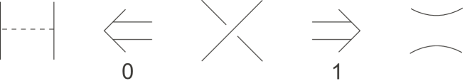
Figure 1. The 0- and 1-resolutions

The set $\Lambda(L)$ of Khovanov basis elements has several grading on it.

Let $n$ (respectively, $n_{+}$, $n_{-}$) be the number of crossings (respectively, positive crossings, negative crossings) of $L$.

For a labeled resolution configurations $(D_{L}(u),x)\in\Lambda(L)$, its homological grading is

(1.1) $$\mathrm{gr}_{h}(D_{L(u)},x)=-n_{-}+|u|,$$

and the quantum grading is

(1.2) $$\mathrm{gr}_{q}(D_{L}(u),x)=n_{+}-2n_{-}+|u|+\sharp\{Z\in Z(D_{L}(u))|x(Z)=x_{+}\}-\sharp\{Z\in Z(D_{L}(u))|x(Z)=x_{-}\}.$$

Let us consider the set $\mathfrak{L}=[S^{1};F]$ of all the homotopy classes of free oriented loops in $F$. Let $\bigcirc\in\mathfrak{L}$ be the homotopy class of contractible loops. For any closed curve $\gamma$, one can consider the curve $-\gamma$ obtained from $\gamma$ by the orientation change. Let $\mathfrak{H}$ be the quotient group of the free abelian group with generator set $\mathfrak{L}$ modulo the relations $\bigcirc=0$ and $[\gamma]=[-\gamma]$ for all free loops $\gamma$.

Define the homotopical grading of the Khovanov basis element $(D_{L}(u),x)$ as follows

(1.3) $$\mathrm{gr}_{\mathfrak{H}}(D_{L}(u),x)=\sum_{Z\in Z(D_{L}(u))}\deg x(Z)\cdot[Z]\in\mathfrak{H},$$

where $\deg(x_{\pm})=\pm 1$.

Definition 1.4.

Given a resolution configuration $D$ and a subset $A^{\prime}\subseteq A(D)$ there is a new resolution configuration $s_{A^{\prime}}(D)$, the surgery of $D$ along $A^{\prime}$, obtained as follows. The circles $Z(s_{A^{\prime}}(D))$ of $s_{A^{\prime}}(D)$ are obtained by performing embedded surgery along the arcs in $A^{\prime}$; in other words, $Z(s_{A^{\prime}}(D))$ is obtained by deleting a neighborhood of $A^{\prime}$ from $Z(D)$ and then connecting the endpoints of the result using parallel translates of $A^{\prime}$. The arcs of $s_{A^{\prime}}(D)$ are the arcs of $D$ not in $A^{\prime}$, i.e., $A(s_{A^{\prime}}(D))=A(D)-A^{\prime}$.

Let $s(D)=s_{A(D)}(D)$ denote the maximal surgery on $D$.

Definition 1.5.

There is a partial order $\prec$ on labeled resolution configurations defined as follows. We declare that $(E,y)\prec(D,x)$ if:

1. $D$ is obtained from $E$ by surgering along a single arc of $A(E)$

2. The labelings $x$ and $y$ induce the same labeling on $D\cap E=E\cap D$.

3. $\mathrm{gr}_{q}(E,y)=\mathrm{gr}_{q}(D,x)$, $\mathrm{gr}_{\mathfrak{H}}(E,y)=\mathrm{gr}_{\mathfrak{H}}(D,x)$.

The possible cases of the order are drawn in Fig. 2 and 3.

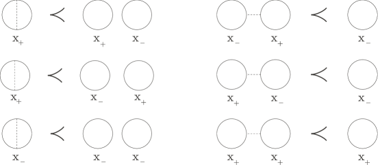
Figure 2. The partial order of labeled resolution configurations with contractible circles

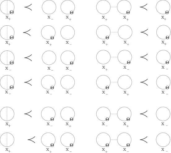
Figure 3. The partial order of labeled resolution configurations with non-contractible circles. Non-contractible circles are marked with (H).

Now, we close the order $\prec$ by transitivity.

Definition 1.6.

Given an oriented link diagram $L$ with $n$ crossings and an ordering of the crossings in $L$, the Khovanov chain complex $KC(L)$ is defined as the $\mathbb{Z}$-module freely generated by labeled resolution configurations of the form $(D_{L}(u),x)$ for $u\in\{0,1\}^{n}$. Thus, the set of all labeled resolution configurations of $L$ is a basis of $KC(L)$.

The Khovanov differential preserves the quantum grading and the homotopical grading, increases the homological grading by 1, and is defined as

(1.4) $${\displaystyle\delta(D_{L}(v),y)=\sum_{(D_{L}(u),x)\succ(D_{L}(v),y)\colon|u|=|v|+1}(-1)^{s_{0}(\mathcal{C}_{u,v})}}(D_{L}(u),x),$$

where for $u=(\epsilon_{1},...,\epsilon_{i-1},1,\epsilon_{i+1},...,\epsilon_{n})$ and $v=(\epsilon_{1},...,\epsilon_{i-1},0,\epsilon_{i+1},...,\epsilon_{n})$, one defines $s_{0}(C_{u,v})=\epsilon_{1}+\cdot\cdot\cdot+\epsilon_{i-1}$.

The homology $KH(L)$ of the complex $(KC(L),\delta)$ are the Khovanov homology of the link $L$.

Definition 1.7.

A decorated resolution configuration is a triple $(D,x,y)$ where $D$ is a resolution configuration and $x$ (respectively, $y$) is a labeling of each component of $Z(s(D))$ (respectively, $Z(D)$) by an element of $\{x_{+},x_{-}\}$. The labeled resolution configuration $i=(D,y)$ is the initial configuration of the decorated resolution configuration, and the labeled resolution configuration $f=(s(D),x)$ is the final configuration.

Associated to a decorated resolution configuration $(D,x,y)$ is the poset $P(D,x,y)$ consisting of all labeled resolution configurations $(E,z)$ with $(D,y)\prec(E,z)\prec(s(D),x)$. We call $P(D,x,y)$ the poset for $(D,x,y)$.

For any resolution configuration $D^{\prime}=s_{A}(D)$, $A\subset A(D)$, we define its multiplicity as the number of its labelings which belong to $P(D,x,y)$:

$$\mu_{(D,x,y)}(D^{\prime})=\sharp\{z\,|\,(D,y)\prec(D^{\prime},z)\prec(s(D),x)\}.$$

The multiplicity $\mu(D,x,y)$ of a decorated resolution configuration $(D,x,y)$ is the maximum of the multiplicities $\mu_{(D,x,y)}(D^{\prime})$:

$$\mu(D,x,y)=\max_{A\subset A(D)}\mu_{(D,x,y)}(s_{A}(D)).$$

Definition 1.8.

The core $c(D)$ of a resolution configuration $D$ is the resolution configuration obtained from $D$ by deleting all the circles in $Z(D)$ that are disjoint from all the arcs in $A(D)$. A resolution configuration $D$ is called basic if $D=c(D)$, that is, if every circle in $Z(D)$ intersects an arc in $A(D)$.

In the same way one can define the core $c(D,x)$ of a labeled resolution configuration $(D,x)$, and basic labeled resolution configurations.

The core of a decorated resolution configuration $(D,x,y)$ is the decorated configuration

$$c(D,x,y)=(c(D),x\mid_{s(c(D))},y\mid_{c(D)}).$$

A decorated resolution configuration is basic if it coincides with its core.

Remark 1.9.

Given two comparable labeled resolution configurations $\alpha=(D,y)\prec(D^{\prime},x)=\beta$, $D^{\prime}=s_{A}(D)$, $A\subset A(D)$, one can assign a basic decorated resolution configuration ${\mathcal{D}}(\alpha,\beta)$ to it. Consider two resolution configurations $\bar{D}=(Z(D),A)$, $\bar{D}^{\prime}=s(\bar{D})=(Z(D^{\prime}),\emptyset)$. Then the decorated configuration ${\mathcal{D}}(\alpha,\beta)$ is defined as the core of $(\bar{D},x,y)$.

If $(D,y)\not\prec(D^{\prime},x)$ we say that the corresponding decorated resolution configuration is empty.

Remark 1.10.

(Basic) decorated resolution configurations form a partially ordered set by inclusion relation: $(D^{\prime},x^{\prime},y^{\prime})\subset(D,x,y)$ if $(D^{\prime},y^{\prime})$ and $(s(D^{\prime}),x^{\prime})$ belong the poset $P(D,x,y)$.

1.2. Khovanov homotopy type

Let us remind the construction of Khovanov homotopy type by R. Lipshitz and S. Sarkar [17].

Definition 1.11.

A $k$-dimensional manifold with corners is a topological space $X$ which is locally homeomorphic to an open subset of $\mathbb{R}^{k}_{+}=(\mathbb{R}_{+})^{k}$ where $\mathbb{R}_{+}=[0,\infty)$.

For $x\in X$, let $c(x)$ be the number of zero coordinates of the corresponding point in $\mathbb{R}^{k}_{+}$. The set $\{x\in X\,|\,c(x)=i\}$ is the codimension-$i$ boundary of $X$.

A connected facet of $X$ is the closure of a connected component of the codimension-$1$ boundary of $X$. A facet is a union of disjoint connected facets.

Definition 1.12.

A manifold with corners $X$ is called a manifold with facets if every point $x\in X$ belongs to exactly $c(x)$ connected facets. An $\langle n\rangle$-manifold is a manifold with facets $X$ along with an ordered $n$-tuple $(\partial_{1}X,\dots,\partial_{n}X)$ of facets of $X$ such that

• $\bigcup_{i=1}^{n}\partial_{i}X=\partial X$;

• for all distinct $i,j$ the intersection $\partial_{i}X\cap\partial_{j}X$ is a facet of both $\partial_{i}X$ and $\partial_{j}X$.

For any $A\subset\{1,\dots,n\}$ denote $X(A)=\bigcap_{i\in A}\partial_{i}X$.

Definition 1.13.

Given a $(n+1)$-tuple ${\mathbf{d}}=(d_{0},\dots,d_{n})\in\mathbb{N}^{n+1}$, let

$$\mathbb{E}^{\mathbf{d}}_{n}=\mathbb{R}^{d_{0}}\times\mathbb{R}_{+}\times\mathbb{R}^{d_{1}}\times\mathbb{R}_{+}\times\dots\times\mathbb{R}_{+}\times\mathbb{R}^{d_{n}}.$$

$\mathbb{E}^{\mathbf{d}}_{n}$ is a $\langle n\rangle$-manifold with

$$\partial_{i}(\mathbb{E}^{\mathbf{d}}_{n})=\mathbb{R}^{d_{0}}\times\dots\times\mathbb{R}^{d_{i-1}}\times\{0\}\times\dots\times\mathbb{R}^{d_{n}}.$$

A neat immersion of an $\langle n\rangle$-manifold is a smooth immersion $\iota\colon X\looparrowright\mathbb{E}_{n}^{\mathbf{d}}$ for some $\mathbf{d}$ such that:

1. $\iota^{-1}(\partial_{i}(\mathbb{E}^{\mathbf{d}}_{n}))=\partial_{i}X$ for all $i$,
   

2. for any $A\subset B\subset\{1,\dots,n\}$ the sets $\iota(X(A))$ and $\mathbb{E}^{\mathbf{d}}_{n}(B)$ are transversal.

A neat embeding is a neat immersion that is also an embedding.

Definition 1.14.

A flow category is a pair $(\mathscr{C},\mathrm{gr})$ where $\mathscr{C}$ is a category with finitely many objects $Ob(\mathscr{C})$ and $\mathrm{gr}\colon Ob(\mathscr{C})\to\mathbb{Z}$ is a function, satisfying the following conditions:

1. $\mathrm{Hom}(x,x)={id}$ for all $x\in Ob(\mathscr{C})$, and for distinct $x,y\in Ob(\mathscr{C})$, $\mathrm{Hom}(x,y)$ is a compact $(\mathrm{gr}(x)-\mathrm{gr}(y)-1)$-dimensional $\langle\mathrm{gr}(x)-\mathrm{gr}(y)-1\rangle$-manifold;

2. for distinct $x,y,z\in Ob(\mathscr{C})$ with $\mathrm{gr}(z)-\mathrm{gr}(y)=m$ the composition map

   $$\circ\colon\mathrm{Hom}(z,y)\times\mathrm{Hom}(x,z)\to\mathrm{Hom}(x,y)$$

   is an embedding into $\partial_{m}\mathrm{Hom}(x,y)$. Furthermore,

   $$\circ^{-1}(\partial_{i}\mathrm{Hom}(x,y))=\left\{\begin{array}[]{cl}\partial_{i}\mathrm{Hom}(z,y)\times\mathrm{Hom}(x,z)&\mbox{for }i<m,\\ \mathrm{Hom}(z,y)\times\partial_{i-m}\mathrm{Hom}(x,z)&\mbox{for }i>m.\end{array}\right.$$

3. for distinct $x,y\in Ob(\mathscr{C})$ the composition induces a diffeomorphism

   $$\partial_{i}\mathrm{Hom}(x,y)\cong\bigsqcup_{z\in Ob(\mathscr{C})\colon\mathrm{gr}(z)=\mathrm{gr}(y)+i}\mathrm{Hom}(z,y)\times\mathrm{Hom}(x,z).$$

For any objects $x,y$ in a flow category define the moduli space from $x$ to $y$ to be

$$\mathcal{M}(x,y)=\left\{\begin{array}[]{cl}\emptyset&\mbox{if }x=y,\\ \mathrm{Hom}(x,y)&\mbox{otherwise}.\end{array}\right.$$

Let ${\mathbf{d}}=(\dots,d_{-1},d_{0},d_{1},\dots)$ be a sequence of natural numbers. For any $a<b$ denote $\mathbb{E}_{\mathbf{d}}[a:b]=\mathbb{E}_{b-a-1}^{d_{a},\dots,d_{b-1}}$.

Definition 1.15.

A neat immersion (embedding) of a flow category $\mathscr{C}$ is a collection of neat immersions (embeddings) $\iota_{x,y}\colon\mathcal{M}(x,y)\looparrowright\mathbb{E}_{\mathbf{d}}[\mathrm{gr}(y):\mathrm{gr}(x)]$ such that

1. for all $i,j$ the map

   $$\iota_{i,j}=\sqcup_{x,y}\iota_{x,y}\colon\bigsqcup_{x,y\in Ob(\mathscr{C})\colon\mathrm{gr}(x)=i,\mathrm{gr}(y)=j}\mathcal{M}(x,y)\to\mathbb{E}_{\mathbf{d}}[j:i]$$

   is a neat immersion (embedding);

2. for all objects $x,y,z$ and all points $p\in\mathcal{M}(x,z)$, $q\in\mathcal{M}(z,y)$

   $$\iota_{x,y}(q\circ p)=(\iota_{z,y}(q),0,\iota_{x,z}(p)).$$

Definition 1.16.

Let $\iota$ be a neat immersion of a flow category $\mathscr{C}$. For objects $x,y$, let $\nu_{x,y}$ be the normal bundle on the moduli space $\mathcal{M}(x,y)$, induced by the immersion $\iota_{x,y}$. A coherent framing $\phi$ of the normal bundle is a framing for $\nu_{x,y}$ for all objects $x,y$ such that the product framing $\nu_{z,y}\times\nu_{x,z}$ equals to the pullback $\circ^{*}(\nu_{x,y})$ for all $x,y,z$.

A flow category with a fixed coherent framing of the normal bundle to some neat immersion is called a framed flow category.

For a framed flow category there is an associated cochain complex $C^{*}(\mathscr{C})$. The chain space of the complex is the free abelian group generated by the objects of the category: $C^{*}(\mathscr{C})=\mathbb{Z}[Ob(\mathscr{C})]$; the differential is given by the formula

$$\delta y=\sum_{x\in Ob(\mathscr{C})\colon\mathrm{gr}(x)=\mathrm{gr}(y)+1}\left(\sum_{f\in\mathcal{M}(x,y)}\phi(f)\right)x.$$

The moduli space in the formula is a compact zero-dimensional manifold, i.e. a finite set, and the framing $\phi$ is given by signs of the elements of that set.

To a framed flow category one can associate a based CW complex in the following way.

Definition 1.17.

Let $\mathscr{C}$ be a framed flow categoty with a neat embedding $\iota$ into $\mathbb{E}_{\mathbf{d}}$ and a framing $\phi$. Let $B=\min_{x\in Ob(\mathscr{C})}\mathrm{gr}(x)$ and $B=\max_{x\in Ob(\mathscr{C})}\mathrm{gr}(x)$.. Using framing, extend the embedding $\iota_{x,y}$ for some small $\epsilon>0$ to an embedding

$$\tilde{\iota}_{x,y}\colon\mathcal{M}(x,y)\times[-\epsilon,\epsilon]^{d_{\mathrm{gr}(y)}+\cdots+d_{\mathrm{gr}(x)-1}}\to\mathbb{E}_{\mathbf{d}}[\mathrm{gr}(y):\mathrm{gr}(x)]$$

where $\mathbb{E}_{\mathbf{d}}[\mathrm{gr}(y):\mathrm{gr}(x)]=\mathbb{R}^{d_{\mathrm{gr}(y)}}\times\mathbb{R}_{+}\times\dots\times\mathbb{R}_{+}\times\mathbb{R}^{d_{\mathrm{gr}(x)-1}}.$

Choose $R$ sufficiently large so that for all $x,y$

$$\tilde{\iota}_{x,y}\colon\mathcal{M}(x,y)\times[-\epsilon,\epsilon]^{d_{\mathrm{gr}(y)}+\cdots+d_{\mathrm{gr}(x)-1}}$$

lies in $[-R,R]^{d_{\mathrm{gr}(y)}}\times[0,R]\times\dots\times[0,R]\times[-R,R]^{d_{\mathrm{gr}(x)-1}}$.

To any object $x$ assign the cell

$$C(x)=[0,R]\times[-R,R]^{d_{B}}\times\dots\times[0,R]\times[-R,R]^{d_{\mathrm{gr}(x)-1}}\times\{0\}\times\\ [-\epsilon,\epsilon]^{d_{\mathrm{gr}(x)}}\times\dots\times\{0\}\times[-R,R]^{d_{A-1}}.$$

For any other object $y$ such that $\mathrm{gr}(y)<\mathrm{gr}(x)$ one identifies $C(y)\times\mathcal{M}(x,y)$ with the subset

$$C_{y}(x)=[0,R]\times[-R,R]^{d_{B}}\times\dots\times[0,R]\times[-R,R]^{d_{\mathrm{gr}(y)-1}}\times\{0\}\times\\ \iota_{x,y}(\mathcal{M}(x,y))\times\{0\}\times[-\epsilon,\epsilon]^{d_{\mathrm{gr}(x)}}\times\dots\times\{0\}\times[-\epsilon,\epsilon]^{d_{A}-1}.$$

Define the attaching map for $C(x)$ as the map which is the projection $C_{y}(x)\cong C(y)\times\mathcal{M}(x,y)$ to $C(y)$ on $C_{y}(x)$ and the map to the basepoint on the $\partial C(x)\setminus\bigcup_{y}C_{y}(x)$.

These gluing maps define a CW complex $|\mathscr{C}|$ which is the Cohen–Jones–Segal realization of the framed flow category $\mathscr{C}$.

Theorem 1.18 ([17]).

The CW complex $|\mathscr{C}|$ is well defined and its cellular cochain complex is isomorphic to the associated cochain complex $C^{*}(\mathscr{C})$.

Example 1.19 (Cube flow category).

Let $X=[0,1]^{n}$ be the $n$-dimensional cube and $f_{n}(x_{1},\dots,x_{n})=f(x_{1})+\cdots+f(x_{n})$, where $f(x)=3x^{2}-2x^{3}$, be a Morse function on it. Define the $n$-dimensional cube flow category $\mathscr{C}_{C}(n)$ as the Morse flow category of the function $f_{n}$. This means that the objects of $\mathscr{C}_{C}(n)$ are the critical points of $f_{n}$, i.e. the vertices $\{0,1\}^{n}$ of the cube $X$.

Denote the object $(0,\dots,0)$ by $\bar{0}$, and the object $(1,\dots,1)$ by $\bar{1}$.

The grading function is defined as $\mathrm{gr}(u)=|u|=\sum_{i=1}^{n}u_{i}$, $u=(u_{1},\dots,u_{n})\in\{0,1\}^{n}$. The moduli space $\mathcal{M}(x,y)$ consists of the lines of the gradient flow which starts at $x$ and ends at $y$. One can identify the moduli space $\mathcal{M}(x,y)$ with the permutahedron of dimension $\mathrm{gr}(x)-\mathrm{gr}(y)-1$.

The cube flow category can be framed (by induction on the moduli spaces dimension).

Example 1.20 (Khovanov flow category).

Let $\mathcal{L}$ in $S^{3}$ be a link and $L$ in $S^{2}$ be its diagram.

The Khovanov flow category $\mathscr{C}_{K}(L)$ has one object for each Khovanov basis element. That is, an object of $\mathscr{C}_{K}(L)$ is a labeled resolution configuration of the form $\mathbf{x}=(D_{L}(u),x)$ with $u\in\{0,1\}^{n}$. The grading on the objects is the homological grading gr_h; the quantum grading gr_q is an additional grading on the objects. We need the orientation of $L$ in order to define these gradings, but the rest of the construction of $\mathscr{C}_{K}(L)$ is independent of the orientation. Consider objects $\mathbf{x}=(D_{L}(u),x)$ and $\mathbf{y}=(D_{L}(v),y)$ of $\mathscr{C}_{K}(L)$. The space $\mathcal{M}_{\mathscr{C}_{K}(L)}(\mathbf{x},\mathbf{y})$ is defined to be empty unless $y\prec x$ with respect to the partial order from Definition 1.5. So, assume that $y\prec x$. Let $x|$ denote the restriction of $x$ to $s(D_{L}(v)-D_{L}(u))=D_{L}(u)-D_{L}(v)$ and let $y|$ denote the restriction of $y$ to $D_{L}(v)-D_{L}(u)$. Therefore, $(D_{L}(v)-D_{L}(u),x|,y|)$ is a basic decorated resolution configuration.

In [17, §5 and §6] Lipshitz and Sarkar associate to each index $n$ basic decorated resolution configuration $(D,x,y)$ an $(n-1)$-dimensional $\left<n-1\right>$-manifold $\mathcal{M}(D,x,y)$ together with a $\mu(D,x,y)$-fold trivial covering

$$\mathcal{F}:\mathcal{M}(D,x,y)\to\mathcal{M}_{\mathscr{C}(n)}(\overline{1},\overline{0}).$$

Use it, and define

$$\mathcal{M}_{\mathscr{C}_{K}(L)}(\mathbf{x},\mathbf{y})=\mathcal{M}(D_{L}(v)-D_{L}(u),x|,y|).$$

The framing of the cube flow category can be lifted to the Khovanov category.

Definition 1.21.

The Cohen–Jones–Segal realization ${\mathcal{X}}(L)=|\mathscr{C}_{K}(L)|$ of the Khovanov framed flow category is called the Khovanov-Lipshitz-Sarkar stable homotopy type of the link diagram $L$.

Theorem 1.22 ([17]).

The Khovanov-Lipshitz-Sarkar stable homotopy type ${\mathcal{X}}(L)$ is a link invariant.

2. Moduli systems

Let $F$ be a closed oriented surface. We consider links in the thickening of the surface $F$. In order to define Khovanov homotopy type of such links we need fix a set of moduli spaces for the decorated resolution configurations of the link. This observation leads to the following definition, cf. [17, Section 5.1].

Definition 2.1.

A branched covering moduli system on the surface $F$ is a family of correspondences between the basic decorated resolution configurations of index $n$ in the surface $F$ and $(n-1)$-dimensional $\langle n-1\rangle$-manifolds:

$$\mathcal{M}\colon(D,x,y)\mapsto\mathcal{M}(D,x,y)$$

together with $\langle n-1\rangle$-maps

$$\mathcal{F}_{(D,x,y)}\colon\mathcal{M}(D,x,y)\to\mathcal{M}_{\mathcal{C}_{C}(n)}(\bar{1},\bar{0})$$

These correspondences must obey the following conditions:

1. the moduli space $\mathcal{M}(D,x,y)$ of a basic decorated resolution configuration $(D,x,y)$ depends only on the isotopy class of the configuration;

2. $\mathcal{M}(D,x,y)=\emptyset$ if $P(D,x,y)=\emptyset$;

3. for any $(E,z)\in P(D,x,y)$ there are embeddings

   $$\circ\colon\mathcal{M}(D\setminus E,z|,y|)\times\mathcal{M}(E\setminus s(D),x|,z|)\to\mathcal{M}(D,x,y);$$

4. the faces of $\mathcal{M}(D,x,y)$ are determined by

   $$\partial_{i}\mathcal{M}(D,x,y)=\coprod_{(E,z)\in P(D,x,y),\ ind(D\setminus E)=i}\circ(\mathcal{M}(D\setminus E,z|,y|)\times\mathcal{M}(E\setminus s(D),x|,z|));$$

5. the composition is compatible with the maps $\mathcal{F}$: for any $E=D_{D}(v)$

6. the map $\mathcal{F}_{(D,x,y)}$ is a $\mu(D,x,y)$-fold branched covering.

Note that we can define the covering by pointing out the branching set $P\subset\mathcal{M}_{\mathcal{C}_{C}(n)}(\bar{1},\bar{0})$ of codimension 2.

Definition 2.2.

The moduli system $\{\mathcal{M}(D,x,y)\}$ is cubical or of type C if all the covering maps over the cubic moduli spaces are trivial. Otherwise, the moduli system is called dodecagonal or of type D.

Theorem 2.3.

1. For any closed oriented surface $F$ there exists a covering moduli system of type $C$.

2. For any closed oriented surface $F$ there exists a covering moduli system of type $D$.

We present the corresponding moduli systems in Sections 4.1 and 4.2

Given a (branched covering) moduli system $\mathcal{M}=\{\mathcal{M}(D,x,y)\}$, let $\mathscr{C}_{\mathcal{M}}(L)$ be the Khovanov flow category whose objects are labeled resolution configurations and moduli spaces are

$$\mathcal{M}((D_{L}(u),x),(D_{L}(v),y))=\mathcal{M}(D_{L}(v)-D_{L}(u),x|,y|).$$

Proposition 2.4.

There is a structure of framed flow category on $\mathscr{C}_{\mathcal{M}}(L)$.

Proof.

Let $\iota_{C}$ be a neat embedding of the cube flow category $\mathcal{C}_{C}$ with a coherent framing $\phi_{C}$. Then $\iota_{0}=\iota_{C}\circ\mathcal{F}$ is a neat map into some $\mathbb{E}_{\mathbf{d}}[a:b]$. Although the map $\iota_{0}$ is not a neat immersion in general, the normal bundle to the image $\iota_{0}(\mathscr{C}_{\mathcal{M}}(L))=\iota_{C}(\mathcal{C}_{C})$ is well-defined and framed (see Fig. 4).

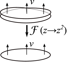
Figure 4. Lifting of a normal framing to a branch cover

By Lemma 3.16 of [17] there exists a neat embedding $\iota_{1}$ of the flow category $\mathscr{C}_{\mathcal{M}}(L)$ into $\mathbb{E}_{\mathbf{d}^{\prime}}[a:b]$. By Lemma 3.17 of [17] there exists a family of neat maps $\tilde{\iota}_{t}$ connecting the neat maps $\iota_{0}[\mathbf{d}+\mathbf{d^{\prime}}+1]$ and $\iota_{1}[\mathbf{d}+\mathbf{d^{\prime}}+1]$ such that for any $t>0$ the map $\tilde{\iota}_{t}$ is a neat embedding. This family of maps admits an explicit formula

$$\tilde{\iota}_{t}\colon\mathscr{C}_{\mathcal{M}}(L)\to\mathbb{E}_{\mathbf{d}+\mathbf{d^{\prime}}+1}[a:b]=\mathbb{R}^{d_{a}+d^{\prime}_{a}+1}\times\mathbb{R}_{+}\times\mathbb{R}^{d_{a+1}+d^{\prime}_{a+1}+1}\times\mathbb{R}_{+}\times\dots\times\mathbb{R}_{+}\times\mathbb{R}^{d_{b-1}+d^{\prime}_{b-1}+1},$$

$$\tilde{\iota}_{t}=((1-t)\iota_{0}^{a}+t\iota_{1}^{a},f(t)\iota_{1}^{a},f(t)\bar{\iota}_{1}^{a+1},(1-t)\bar{\iota}_{0}^{a+1}+t\bar{\iota}_{1}^{a+1},(1-t)\iota_{0}^{a+1}+t\iota_{1}^{a+1},\dots,(1-t)\iota_{0}^{b-1}+t\iota_{1}^{b-1},f(t)\iota_{1}^{b-1},0)$$

where $f(t)=e^{-\frac{1}{t(1-t)}}$ and

$$\iota_{0}=(\iota_{0}^{a},\bar{\iota}_{0}^{a+1},\iota_{0}^{a+1},\dots,\bar{\iota}_{0}^{b-1},\iota_{0}^{b-1})\colon\mathscr{C}_{\mathcal{M}}(L)\to\mathbb{R}^{d_{a}}\times\mathbb{R}_{+}\times\mathbb{R}^{d_{a+1}}\times\dots\times\mathbb{R}_{+}\times\mathbb{R}^{d_{b-1}}.$$

By Lemma 3.19 of [17] we can extend the coherent framing $\phi$ for the map $\tilde{\iota}_{0}=\iota_{0}[\mathbf{d^{\prime}}+\mathbf{d^{\prime\prime}}]$ to a family of coherent framings $\phi_{t}$ for the maps $\tilde{\iota}_{t}$. In particular, the neat embedding $\tilde{\iota}_{1}=\iota_{1}[\mathbf{d}+\mathbf{d^{\prime\prime}}]$ admits the coherent framing $\phi_{1}$. ∎

Define the Khovanov homotopy type ${\mathcal{X}}_{\mathcal{M}}(L)$ associated with the moduli system $\mathcal{M}$ as the realization of the framed flow category $\mathscr{C}_{\mathcal{M}}(L)$.

Theorem 2.5.

Khovanov homotopy type ${\mathcal{X}}_{\mathcal{M}}(L)$ is a link invariant.

Proof.

We can use the reasoning of [17, Propositions 6.2, 6.3, 6.4] without any changes.

Indeed, let the diagram $L^{\prime}$ differ from $L$ by an increasing first Reidemeister move, Fig. 5.

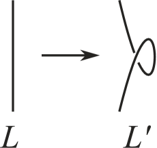
Figure 5. First Reidemeister move

The Khovanov complex of the diagram $L^{\prime}$ contains a contractible subcomplex $C_{1}$, Fig. 6 left. The quotient complex $C_{2}$ (Fig. 6 right) can be identified with the Khovanov complex of $L$. On the level of flow category this means that the Khovanov flow category $\mathscr{C}_{K}(L)$ contains a closed subcategory $\mathscr{C}_{1}$ which corresponds to $C_{1}$ and a subcategory $\mathscr{C}_{2}$ that corresponds to $C_{2}$. The subcategory $\mathscr{C}_{2}$ is isomorphic to the category $\mathscr{C}_{K}(L)$. The geometric realization of $\mathscr{C}_{1}$ is contractible, hence, ${\mathcal{X}}_{\mathcal{M}}(L^{\prime})=|\mathscr{C}_{K}(L^{\prime})|=|\mathscr{C}_{1}|\vee|\mathscr{C}_{2}|=|\mathscr{C}_{2}|=|\mathscr{C}_{K}(L)|={\mathcal{X}}_{\mathcal{M}}(L)$.

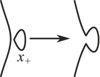
Figure 6. Parts of Khovanov complex of the diagram $L^{\prime}$

Analogously, one establishes the invariance under the second and third Reidemeister moves. ∎

2.1. Multivalued moduli systems

Definition 2.6.

A multivalued moduli system is a correspondence between basic decorated resolution configurations of index $n$ and sets of $(n-1)$-dimensional $\langle n-1\rangle$-manifolds ${\mathfrak{M}}(D,x,y)$. We reformulate the boundary condition as follows: for any $\mathcal{M}\in{\mathfrak{M}}(D,x,y)$

$$\partial_{i}\mathcal{M}=\coprod_{(E,z)\in P(D,x,y),\ ind(D\setminus E)=i}\circ(\mathcal{M}_{D\setminus E}\times\mathcal{M}_{E\setminus s(D)}),$$

for some $\mathcal{M}_{D\setminus E}\in{\mathfrak{M}}(D\setminus E,z|,y|)$, $\mathcal{M}_{E\setminus s(D)}\in{\mathfrak{M}}(E\setminus s(D),x|,z|)$.

A multivalued moduli system is extendable if for any decorated resolution configuration $(D^{\prime},z,w)$ and any choice of moduli spaces $M(D,x,y)\in{\mathfrak{M}}(D,x,y)$ for all the proper decorated resolution sub-configurations $(D,x,y)\subsetneq(D^{\prime},z,w)$ which satisfies the conditions (2)-(6) of Definition 2.1, there exists $M(D^{\prime},z,w)\in{\mathfrak{M}}(D^{\prime},z,w)$ such that

$$\partial_{i}M(D^{\prime},z,w)=\coprod_{(E,x)\in P(D^{\prime},z,w),\ ind(D^{\prime}\setminus E)=i}\circ(M{(D^{\prime}\setminus E,x,w)}\times M{(E\setminus s(D^{\prime}),z,x)}),$$

.

In other words, any compatible choice of moduli spaces of the proper decorated resolution sub-configurations can be extended to a compatible choice of a moduli space for the whole decorated resolution configuration.

Theorem 2.7.

There exists an extendable multi-valued moduli system.

Note that since any branched covering moduli system is an example of a multivalued moduli system with moduli sets ${\mathfrak{M}}(D,x,y)$ consisting at most of one moduli space, Theorem 2.3 implies Theorem 2.7. In particular, the moduli systems of types (C) and (D) constructed in Sections 4.1 and 4.2 are multivalued moduli systems. In Section 4.3 we present a multivalued moduli systems which assigns several spaces to decorated resolution configurations.

Using a multi-valued moduli system, one can construct a framed flow category by choosing moduli spaces $\mathcal{M}_{D}\in{\mathfrak{M}}(D,x,y)$ for each decorated resolution configuration. The geometric realization of this flow category is a topological space which can be thought of as a value of Khovanov homotopy type. By considering all possible choices we get a multivalued Khovanov homotopy type ${\mathfrak{X}}_{\mathfrak{M}}(L)$ which is a set of CW complexes considered up to stable homotopy.

Theorem 2.8.

Let $\mathfrak{M}$ be an extendable multivalued moduli system. Then the multivalued Khovanov homotopy type ${\mathfrak{X}}_{\mathfrak{M}}(L)$ is a link invariant.

Proof.

We need to prove that the set ${\mathfrak{X}}_{\mathfrak{M}}(L)$ is invariant under the Reidemeister moves. Let $L$ and $L^{\prime}$ be two diagrams connected by a Reidemeister move. Take a homotopy type $\mathcal{X}\in{\mathfrak{X}}_{\mathfrak{M}}(L)$. We must find a homotopy type $\mathcal{X}^{\prime}\in{\mathfrak{X}}_{\mathfrak{M}}(L^{\prime})$ which is stable homotopic to $\mathcal{X}$. If the move is an increasing first or second Reidemeister move then the moduli spaces of a Khovanov flow category $\mathscr{C}_{K}(L)$ which produces the CW complex $\mathcal{X}$ can be extended to some moduli spaces for the decorated resolution configurations in a Khovanov flow category $\mathscr{C}_{K}(L^{\prime})$. We can take these moduli spaces and construct a Khovanov homotopy type $\mathcal{X}^{\prime}$. Then the flow category $\mathscr{C}_{K}(L)$ is a subcategory in the flow category $\mathscr{C}_{K}(L^{\prime})$, and $\mathcal{X}$ is embedded in $\mathcal{X}^{\prime}$ (or some factor-space of $\mathcal{X}^{\prime}$) This map induces isomorphism in cohomology. Hence, by Whitehead theorem $\mathcal{X}$ homotopic to $\mathcal{X}^{\prime}$.

For the third Reidemeister move, we consider its braid-like version (see Fig. 7). The left diagram $L$ can be obtained by smoothing the right diagram $L^{\prime}$. Hence, the resolution cube for $L$ is a subcube in the resolution cube for $L^{\prime}$. Then we can use the reasonings above to construct a map between the stable homotopy types or the diagrams which will be a homotopy equivalence by Whitehead theorem.

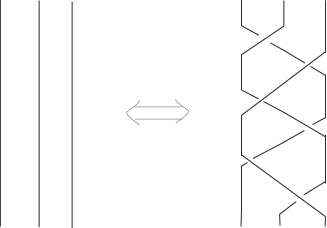
Figure 7. The braid-like Reidemeister move $III$

Thus, for any homotopy type $\mathcal{X}\in{\mathfrak{X}}_{\mathfrak{M}}(L)$ we can extend the corresponding framed flow category to a framed flow category of $L^{\prime}$ and get a homotopy type $\mathcal{X}^{\prime}\in{\mathfrak{X}}_{\mathfrak{M}}(L^{\prime})$ such that $\mathcal{X}\simeq\mathcal{X}^{\prime}$. On the other hand, for a homotopy type $\mathcal{X}^{\prime}\in{\mathfrak{X}}_{\mathfrak{M}}(L^{\prime})$ the restriction of its framed flow category to the resolution configurations of the link $L$ gives a homotopy type $\mathcal{X}\in{\mathfrak{X}}_{\mathfrak{M}}(L)$ such that $\mathcal{X}\simeq\mathcal{X}^{\prime}$. ∎

3. Decorated resolution configurations

Let $F$ be a closed oriented surface. Let us describe decorated resolution configurations of link diagrams in the surface $F$ in more details.

Let $\mathcal{D}=(D,x,y)$ be a decorated resolution configuration in $F$. It is a trivalent graph $F$ consisting of cycles and arcs between the cycles.

Recall that $P(D,x,y)$ is the partially ordered set consisting of the labeled resolution configurations between $(D,y)$ and $(s(D),x)$.

Let $A=A(D)$ be the set of arcs. Assuming the arcs are ordered, there is a map $\pi\colon P(D,x,y)\to C_{n}$, where $n=|A|$ is the index of $D$ and $C_{n}\simeq\{0,1\}^{n}$ is the vertex set of $n$-dimensional cube. If $(s_{A^{\prime}}(D),z)\in P(D,x,y)$ where $A^{\prime}\subset A=\{a_{i}\}_{i=1,\dots,n}$ then one sets $\pi(s_{A^{\prime}}(D),z)=\chi_{A}=(\epsilon_{1},\dots,\epsilon_{n})$ where $\epsilon_{i}=1$ if $a_{i}\in A^{\prime}$ and $\epsilon_{i}=0$ if not.

Recall that the multiplicity of the decorated resolution configuration is the number $\mu(D,x,y)=\max_{v\in C_{n}}|\pi^{-1}(v)|$.

Let $\mathcal{D}_{i}=(D_{i},x|_{D_{i}},y|_{D_{i}})$, $i=1,...,l$ be the connected components of the decorated resolution configuration $(D,x,y)$.

Proposition 3.1.

$\mu(\mathcal{D})=\mu(\mathcal{D}_{1})\times\cdots\times\mu(\mathcal{D}_{l})$.

Proof.

Indeed, for each component $\mathcal{D}_{i}$ we can take a vector $v_{i}$ with the maximal preimage $\pi^{-1}|_{\mathcal{D}_{i}}(v_{i})$. Then the concatenation $v$ of the vectors $v_{1},\dots,v_{l}$ gives the maximal preimage of the map $\pi$, and $|\pi^{-1}(v)|=\prod_{i=1}^{l}\left|\pi^{-1}|_{\mathcal{D}_{i}}(v_{i})\right|$. ∎

Below we assume that the decorate resolution configuration $D$ is connected.

Let $(D,y)$ be a labeled resolution configuration. Denote the number of circles in $D$ by $\gamma(D)$, and let $|y|$ be the sum of labels of the circles. Then $-\gamma(D)\leq|y|\leq\gamma(D)$. The quantum degree of the enchanced state $(D,y)$ is equal to $|\pi(D)|+|y|=|y|$. Let $A^{\prime}\subset A(D)$ and $(s_{A^{\prime}}(D),z)\succ(D,y)$. Since the quantum degrees of comparable configurations coincide, $|y|=|\pi(s_{A^{\prime}}(D))|+|z|=|A^{\prime}|+|z|$. Hence, $-\gamma(s_{A^{\prime}}(D))\leq|z|=|y|-|A^{\prime}|$ and $\gamma(s_{A^{\prime}}(D))\geq|A^{\prime}|-|y|$.

In particular, if $\gamma(D)=1$ and $|y|=-1$ then $\gamma(s_{A^{\prime}}(D))\geq|A^{\prime}|+1$, hence, $\gamma(s_{A^{\prime}}(D))=|A^{\prime}|+1$. If $\gamma(D)=1$ and $|y|=1$ then $\gamma(s_{A^{\prime}}(D))=|A^{\prime}|\pm 1$.

Proposition 3.2.

Let $a\in A(D)$ be a leaf or coleaf (see Fig. 8). Then there exists a unique labeled resolution configuration $(s_{a}(D),z)$ such that $(D,y)\prec(s_{a}(D),z)\prec(s(D),x)$, and

$$P(D,x,y)=P(s_{a}(D),z,y)\times\{0,1\}.$$

Figure 8. Leaf (left) and coleaf (right) in a resolution configuration

Proof.

If $a$ is a leaf then $(s_{a}(D),z)$ is uniquely determined. If $a$ is a coleaf then $s_{a}(D)$ splits into two components $(D_{1},z_{1})$ and $(D_{2},z_{2})$. Then $s(D)=s(D_{1})\sqcup s(D_{2})$. The ambiguity of $z_{1},z_{2}$ concerns the labels of the circles incident to $a$. But one can restore the labels using the quantum grading of the component: $|\pi(D_{i})|+|z_{i}|=|\pi(s(D_{i}))|+|x|_{s(D_{i})}|$, so $|z_{i}|=|\pi(s(D_{i}))|+|x|_{s(D_{i})}|-|\pi(D_{i})|$. If one knows the labels of all the circles in $(D_{i},z_{i})$ except one and the sum of all labels $|z_{i}|$, then the last label is uniquely determined.

Let $P_{0}=\{(s_{A}(D),u)\in P(D,x,y)\,|\,a\not\in A\}$ and $P_{1}=\{(s_{A}(D),u)\in P(D,x,y)\,|\,a\in A\}$. Using the reasonings above, we can prove that the surgery $s_{a}$ establishes an bijection between $P_{0}$ and $P_{1}=P(s_{a}(D),z,y)$. This bijection is compatible with the order in $P_{0}$ and $P_{1}$. ∎

Let $(D,x,y)$ be a nonempty decorated resolution configuration with one circle. Then $D$ is a chord diagram. Let $M=(m_{ab})_{a,b\in A(D)}$ be the $\mathbb{Z}_{2}$-valued interlacement matrix: $m_{ab}=lk(a,b)$, that is $m_{ab}=1$ if the arcs $a$ and $b$ are linked, and $m_{ab}=0$ if they are not. Then $M$ is a skew-symmetric matrix.

For any labeled resolution $(s_{A^{\prime}}(D),z)\in P(D,x,y)$ the number of circles $\gamma(s_{A^{\prime}}(D))$ is given by the curcuit-nullity formula

Proposition 3.3.

$\gamma(s_{A^{\prime}}(D))=corankM|_{A^{\prime}}+1$.

On the other hand, the quantum degree gives the equality $|z|+|A^{\prime}|=|y|$, so $\gamma(s_{A^{\prime}}(D))\geq|A^{\prime}|-|y|$.

If $|y|=-1$ then $\gamma(s_{A^{\prime}}(D))=|A^{\prime}|+1$ and all labels in $z$ are equal to $x_{-}$. Thus, $\mu(D,x,y)=1$.

If $|y|=1$ then $\gamma(s_{A^{\prime}}(D))\geq|A^{\prime}|-1$. Hence,

$$rankM|_{A^{\prime}}=|A^{\prime}|-corankM|_{A^{\prime}}=|A^{\prime}|-\gamma(s_{A^{\prime}}(D))+1\leq 2.$$

In particular, $rankM\leq 2$. Since, $M$ is skew-symmetric then $rankM$ is even.

If $rankM=0$ then $M=0$ and all the arcs are coleafs. Thus, $\mu(D,x,y)=1$.

If $rankM=2$ then there are two independent vectors $a,b\in\mathbb{Z}_{2}^{n}$ such that any row of the matrix is equal to $0,a,b$ or $a+b$. This means the arcs of the chord diagram split into four subsets: three sets of parallel chords and coleaves, see Fig. 9. Then $A(D)=A_{a}\sqcup A_{b}\sqcup A_{a+b}\sqcup A_{0}$.

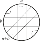
Figure 9. Combinatorial structure of a non empty decorated resolution configuration with one circle

Proposition 3.4.

Let $(D,x,y)$ be a non empty decorated resolution configuration with one circle such that its interlacement matrix has $rankM=2$. Then

1. the circle of the configuration $D$ is contractible

2. the arcs which belong to one subset $A_{a},A_{b},A_{a+b}$ are homotopical in $F$.

Proof.

1. Assume $D$ is not contractible. Take arcs $a\in A_{a}$, $b\in A_{b}$. Let $D^{\prime}=s_{\{a,b\}}(D)$. Then $D$ has label $x_{+}$ and $D^{\prime}$ has label $x_{-}$, hence, $\mathrm{gr}_{\mathfrak{H}}(D,x_{+})=[D]$ and $\mathrm{gr}_{\mathfrak{H}}(D^{\prime},x_{-})=-[D^{\prime}]$. But $[D]\neq-[D^{\prime}]$.

2. Let $a_{1},a_{2}\in A_{a}$ be two non homotopical arcs, and $b\in A_{b}$. Then the resolution $s_{\{a_{1},a_{2},b\}}(D)$ consists of two circles of homotopy type $[a_{1}b^{\pm}a_{2}^{-1}b^{\mp}]$ and $[a_{1}^{-1}a_{2}]$ with labels $x_{-},x_{-}$. Then the homotopical grading of this labeled resolution can not be zero. But $\mathrm{gr}_{\mathfrak{H}}(D,x_{+})=0$ because $D$ is contractible. ∎

Let $(D,x,y)$ be a non empty decorated resolution configuration with one circle such that its interlacement matrix has $rankM=2$. The complement to the circle of the resolution configuration consists of two components, one of which is contractible. We will call an arc inner if it lies in the contractible component, and outer otherwise.

Proposition 3.5.

Let $(D,x,y)$ be a non empty decorated resolution configuration with one circle such that its interlacement matrix has $rankM=2$. Then

1. the arcs from one of the subsets $A_{a},A_{b},A_{a+b}$ are either all inner or all outer

2. let the subsets $A_{a},A_{b}$ consist of outer arcs. Then the surface $F$ is the torus, and the homology type of the arcs in $A_{a+b}$ (when $A_{a+b}\neq\emptyset$) is the sum of homology classes of an arc in $A_{a}$ and an arc $A_{b}$.

3. let the subset $A_{a}$ consist of inner arcs. Then $A_{b}$ consists of outer arcs and $A_{a+b}=\emptyset$.

Proof.

1. Assume that $a_{1},a_{2}\in A_{a}$ and $b\in A_{b}$. Since $a_{i}$, $i=1,2$, and $b$ are interlaced and do not intersect, then these chords lie in different components to the circle of $D$. Hence, the chords $a_{1}$ and $a_{2}$ lie in one component, i.e. they are both internal or both external. Thus, the chords from the subset $A_{a}$ are all internal or all external. The same statements holds for the subsets $A_{b}$ and $A_{a+b}$.

2. Let $a\in A_{a}$ and $b\in A_{b}$ be outer chords. The intersection index of the loops $a$ and $b$ is equal to $1$, hence, $a$ and $b$ present independent homology classes. The resolution configuration $s_{\{a,b\}}(D)$ consists of one circle with the label $x_{-}$. This circle must be contractible due to the homotopical grading. Hence, the surface $F$ can be obtained by gluing two disc along the arcs $a$ and $b$. Thus, $F$ is the torus. Let $c\in A_{a+b}$. Since $c$ is disjoint from $a$ and $b$ and $F$ is the torus, the homology class corresponding to $c$ is equal to $a\pm b$, i.e. it is the sum of the homology classes of $a$ and $b$ (up to signs).

2. Let $a\in A_{a}$ be inner and $b\in A_{b}$ and $c\in A_{a+b}$. Then $b$ and $c$ are outer chords. The intersection index of the loops $b$ and $c$ is equal to $1$, hence, $b$ and $c$ present independent homology classes. The resolution configuration $s_{\{a,b,c\}}(D)$ consists of two circles with the labels $x_{-}$. Then the homotopical grading of this labeled resolution is equal $-2[bc^{-1}]\neq 0$ but the initial resolution configuration has homotopical grading $0$. Thus, the decorated resolution configuration must be empty. ∎

Note that the necessary conditions of Propositions 3.4, 3.5 are also sufficient for the decorated resolution configuration to be non empty.

Proposition 3.6.

1. The multiplicity of a resolution configuration $s_{A^{\prime}}(D)$ is equal to $2$ if $A^{\prime}$ contains chords from exactly one of subsets $A_{a},A_{b},A_{a+b}$, and is equal to $1$ otherwise.

2. Let $(D^{\prime},z,w)\subset(D,x,y)$ be a decorated resolution configuration with an initial configuration $(s_{A^{\prime}}(D),w)$ and final configuration $(s(A^{\prime\prime}),z)$, where $D^{\prime}=s_{A^{\prime}}(D)$ and $A^{\prime}\subset A^{\prime\prime}\subset A(D)$. Then $\mu(D^{\prime},z,w)=2$ if and only if $A^{\prime}\subset A_{0}$ and $A^{\prime\prime}$ intersects at least two of the subsets $A_{a}$, $A_{b}$, $A_{a+b}$.

Proof.

1) Let $A^{\prime}\subset A(D)$. If $A^{\prime}$ does not intersect with $A_{a},A_{b},A_{a+b}$ then it contains only coleaf arcs. The resolution configuration $s_{A^{\prime}}(D)$ consists of circles among which only one contains a pair of linked arcs. Then the label of this circle in $s_{A^{\prime}}(D)$ must be $x_{+}$ (otherwise the surgery by the pair of linked arcs gives zero) whereas the labels of the other circles must be $x_{-}$. Thus, the labels of the configuration $s_{A^{\prime}}(D)$ are defined uniquely, and $\mu(s_{A^{\prime}}(D))=1$.

If $A^{\prime}$ contains a pair arcs from different subsets $A_{a},A_{b},A_{a+b}$ then $rankM|_{A^{\prime}}=2$. This means that the labels of all the circles in $s_{A^{\prime}}(D)$ are $x_{-}$. Thus, $\mu(s_{A^{\prime}}(D))=1$.

If $A^{\prime}$ contains chords from exactly one of subsets $A_{a},A_{b},A_{a+b}$ then the resolution configuration looks like in Fig. 10. There are two circles connected with an arc in $s_{A^{\prime}}(D)$. Hence, the label of one of these circle must be $x_{+}$. The labels of the other circles are $x_{-}$. Hence, the multiplicity is $2$.

Figure 10. Labelings of a resolution configuration of multiplicity $2$

2) The condition of the second statement means the decorated configuration $(D^{\prime},z,w)$ contains a resolution configuration of multiplicity $2$. Thus, it follows from the first statement of the proposition.

∎

Let us now consider resolution configurations with several circles in the initial state.

Let $(D,x,y)$ be a connected nonempty decorated resolution configuration with $k\geq 1$ circles in the initial state. Then there are $k-1$ arcs $\hat{A}=\{c_{1},\dots,c_{k-1}\}\in A(D)$ such that the resolution $D^{\prime}=s_{\hat{A}}(D)$ consists of one circle (Fig. 11). In the diagram $D^{\prime}$ we can draw the arc adjoint to the arcs of $\hat{A}$. With some abuse of notation, we denote the set of the adjoint arcs by $\hat{A}$. Then $D=s_{\hat{A}}(D^{\prime})\cup\hat{A}$.

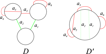
Figure 11. Decorated resolution configurations $D$ and $D^{\prime}$. The set $\hat{A}$ consists of green arcs

Let $M$ be the interlacement matrix of the chords $A(D^{\prime})\cup\hat{A}\simeq(A(D)\setminus\hat{A})\cup\hat{A}=A(D)$ on the circle $D^{\prime}$. Then for any $A^{\prime}\subset A(D)$ the number circles in the resolution configuration is equal to $corankM|_{A^{\prime}\bigtriangleup\hat{A}}+1$ where $A^{\prime}\bigtriangleup\hat{A}$ is the symmetric difference of the sets $A^{\prime}$ and $\hat{A}$.

Proposition 3.7.

Let $(D,x,y)$ be a connected nonempty decorated resolution configuration such that $rankM|_{A(D)\setminus\hat{A}}=2$ and $A^{\prime}\subset A(D)$. Let $M_{A^{\prime}}$ be the submatrix of the interlacement matrix $M$ whose rows correspond to the subset $A^{\prime}\setminus\hat{A}$ and columns correspond to the subset $A(D)\setminus(A^{\prime}\cap\hat{A})$, and $M^{0}_{A^{\prime}}$ be the submatrix with rows from $A^{\prime}\setminus\hat{A}$ and columns from $\hat{A}\setminus A^{\prime}$. Then the resolution configuration $s_{A^{\prime}}(D)$ has in $(D,x,y)$ multiplicity $2$ if and only if $rankM_{A^{\prime}}-rankM^{0}_{A^{\prime}}=1$, and multiplicity $1$ otherwise.

Proof.

The matrix $M_{A^{\prime}}$ includes $M_{A^{\prime}}^{0}$, so $rkM_{A^{\prime}}-rkM^{0}_{A^{\prime}}\geq 0$.

Let $\tilde{D}=s_{\hat{A}\cap A^{\prime}}(D)$ be the resolution configuration obtained from $D$ by surgery along arcs in $\hat{A}$. The resolution configuration $\tilde{D}$ has $|\hat{A}\setminus A^{\prime}|+1$ circles with labels $x_{+}$.

Assume that $rkM^{0}_{A^{\prime}}=0$. This means that the resolution configuration $\tilde{D}$ consists of $|\hat{A}\setminus A^{\prime}|+1$ distinct components.

The chords from different components are not interlaced, i.e. the coefficient correspondent to them in the matrix $M_{A^{\prime}}$ is zero. Indeed, let $c$ and $c^{\prime}$ belong to different components. Then the resolution configuration $s_{\{c,c^{\prime}\}}(\tilde{D})$ has $|\hat{A}\setminus A^{\prime}|+3$ circles, and the resolution configuration $s_{\{c,c^{\prime}\}\cup(\hat{A}\setminus A^{\prime})}(\tilde{D})$ has $|\hat{A}\setminus A^{\prime}|+3-|\hat{A}\setminus A^{\prime}|=3$ circles. But the number of circles is equal to $corankM(\{c,c^{\prime}\})+1$. Hence, $corankM(\{c,c^{\prime}\})=2$ and $M(\{c,c^{\prime}\})=0$, so $m_{cc^{\prime}}=0$.

Among the components of $\tilde{D}$ only one can include interlaced chords. Indeed, if we have pairs $c_{1},c_{1}^{\prime}$ and $c_{2},c_{2}^{\prime}$ of interlaced chords from different component then the surgery $s_{\{c_{1},c_{1}^{\prime},c_{2},c_{2}^{\prime}\}\cup(\hat{A}\setminus A^{\prime})}(\tilde{D})$ would give a resolution configuration with one circle and a label of degree $-2$, but $\deg(x_{-})=-1$ is the minimal grading. Thus, the label is zero and the decorated resolution configuration $(D,x,y)$ is empty.

Thus, we have only one component with interlaced chord. For the matrix $M(A^{\prime})$ this means that its nonzero elements can correspond only to the distinguished component. Thus, $rkM_{A^{\prime}}$ is equal to the rank of the submatrix which corresponds to the component with interlaced chords. Then the statement of the proposition follows from Proposition 3.6.

If $rkM^{0}_{A^{\prime}}>0$ then there are chords in $\tilde{D}$ that connect different circles. Then we can chose subsets $A^{\prime\prime}\subset A^{\prime}$ and $\hat{A}^{\prime\prime}\subset\hat{A}\setminus A^{\prime}$ such that $|A^{\prime\prime}|=|\hat{A}^{\prime\prime}|=rankM^{0}_{A^{\prime}}$ and surgery along the set $\hat{A}\setminus(A^{\prime}\cup\hat{A}^{\prime\prime})\cup A^{\prime\prime}$ transforms the resolution configuration $\tilde{D}$ to a configuration with one circle. Let $\hat{A}_{1}=(\hat{A}\setminus\hat{A}^{\prime\prime})\cup A^{\prime\prime}$ and $M^{\prime}$ be the interlacement matrix on the circle $D_{1}=s_{\hat{A}_{1}}(D)$. Then one can check that $corankM|_{A^{\prime}\bigtriangleup\hat{A}}=corankM^{\prime}|_{A^{\prime}\bigtriangleup\hat{A}_{1}}$, $rankM_{A^{\prime}}-rankM^{0}_{A^{\prime}}=rankM^{\prime}_{A^{\prime}}-rank(M^{\prime})^{0}_{A^{\prime}}$ and $rank(M^{\prime})^{0}_{A^{\prime}}=0$. Thus, the statement of the proposition reduces to the case considered above.

∎

Example 3.8.

Consider the resolution configuration in Fig. 11. With labels $x_{+}$ on each circle, it defines an initial labeled resolution configuration of a decorated resolution configuration. One can choose the set $\hat{A}=\{a_{1},a_{2}\}$ to merge the circles of the configuration. The interlacement matrix then is equal to

$$M=\left(\begin{array}[]{cccccc}0&0&1&0&0&0\\ 0&0&1&0&0&0\\ 1&1&0&0&0&0\\ 0&0&0&0&1&0\\ 0&0&0&1&0&0\\ 0&0&0&0&0&0\end{array}\right).$$

Consider the surgery along the subset $A^{\prime}=\{a_{1},a_{3},a_{5},a_{6}\}$. The matrix $M_{A^{\prime}}$ is equal

$$M_{A^{\prime}}=\left(\begin{array}[]{c|ccc}1&0&0&0\\ 0&0&1&0\\ 0&0&0&0\end{array}\right)$$

where the left part is the submatrix $M^{0}_{A^{\prime}}$. Then $rankM_{A^{\prime}}=2$ and $rankM^{0}_{A^{\prime}}=1$. Since $rankM_{A^{\prime}}-rankM^{0}_{A^{\prime}}=1$, the multiplicity of the resolution configuration $s_{A^{\prime}}(D)$ is equal to $2$. The labelings of the resolution configuration $s_{A^{\prime}}(D)$ are shown in Fig. 12.

Figure 12. Resolution configuration $s_{\{a_{1},a_{3},a_{5},a_{6}\}}(D)$ and its labelings

Let us enumerate the isotopy classes of connected decorated resolution configuration of multiplicity $>1$.

3.1. Decorated resolution configurations of index $1$

All nonempty decorated resolution configurations consists of a comparable pair of labeled resolution configurations and have multiplicity $1$.

3.2. Decorated resolution configurations of index $2$

According to Propositions 3.6 and 3.7 the multiplicity of a decorated resolution configuration $(D,x,y)$ with two arcs is equal to $1$ except three cases (see Fig. 13).

If $F=S^{2}$ then there is a unique up to isomorphism decorated resolution configuration $L_{0}$ of multiplicity $2$. When $F\neq T^{2}$, the decorated resolution configurations of multiplicity $2$ are the ladybug resolution configuration of type $L_{\alpha}$ where $\alpha$ is a homotopy class of a nontrivial simple loop in $F$. In the torus case $F=T^{2}$, there is a two-parameter series of decorated resolution configurations of multiplicity $2$. The parameters are two homology classes $\alpha$ and $\beta$ in $H_{1}(T^{2})$.

Figure 13. Ladybug configurations of type $L_{0}$ (left) and $L_{\alpha}$ (middle), and a quasi-ladybug configuration of type $Q_{\alpha,\beta}$ (right). The labels of the circles are $x_{+}$

Let us consider these configuration more attentively.

3.2.1. The ladybug configuration for link diagrams in $S^{2}$

We review the ladybug configuration for link diagrams in $S^{2}$, which is introduced in [17, section 5.4]. Lipshitz and Sarkar introduced it in the case of link diagrams in $S^{2}$. We cite the definition of it, that of the right pair, and that of the left pair associated with it from [17, section 5.4.2].

Definition 3.9.

([17, Definition 5.6]). An index 2 basic resolution configuration $D$ in $S^{2}$ is said to be a ladybug configuration if the following conditions are satisfied (See Figure 14.).

$\bullet$ $Z(D)$ consists of a single circle, which we will abbreviate as $Z$;

$\bullet$ The endpoints of the two arcs in $A(D)$, say $A_{1}$ and $A_{2}$, alternate around $Z$

(that is, $\partial A_{1}$ and $\partial A_{2}$ are linked in $Z$).

Definition 3.10.

([17, section 5.4.2]). Let $D$ be as above. Let $Z$ denote the unique circle in $Z(D)$. The surgery $s_{A_{1}}(D)$ (respectively, $s_{A_{2}}(D)$) consists of two circles; denote these $Z_{1,1}$ and $Z_{1,2}$ (respectively, $Z_{2,1}$ and $Z_{2,2}$); that is, $Z(s_{A_{i}}(D))=\{Z_{i,1},Z_{i,2}\}$.

As an intermediate step, we distinguish two of the four arcs in $Z-(\partial A_{1}\cup\partial A_{2})$. Assume that the point $\infty\in S^{2}$ is not in $D$, and view $D$ as lying in the plane $S^{2}-\{\infty\}\cong\mathbb{R}^{2}$. Then one of $A_{1}$ or $A_{2}$ lies outside $Z$ (in the plane) while the other lies inside $Z$. Let $A_{i}$ be the inside arc and $A_{o}$ the outside arc. The circle $Z$ inherits an orientation from the disk it bounds in $\mathbb{R}^{2}$. With respect to this orientation, each component of $Z-(\partial A_{1}\cup\partial A_{2})$ either runs from the outside arc $A_{o}$ to an inside arc $A_{i}$ or vice-versa. The right pair is the pair of components of $Z-(\partial A_{1}\cup\partial A_{2})$ which run from the outside arc $A_{o}$ to the inside arc $A_{i}$. The other pair of components is the left pair. See [17, Figure 5.1].

We explain why the ladybug configuration is important, below.

Proposition 3.11.

Let ${\bf x}$ $($respectively, ${\bf y})$ be a labelled resolution configuration in $S^{2}$ of homological grading $n$ $($respectively, $n+2).$ Then the cardinality of the set

$\{p|p$ is a labelled resolution configuration. ${\bf x}\prec p,p\prec{\bf y},$ $p\neq{\bf x}$, $p\neq{\bf y}\}$

is 0, 2, or 4, where $\prec$ represents the partial order defined in [17, Definition 2.10].

Let $D$ be the ladybug configuration in $S^{2}$. Since each of $D$ and $s(D)$ has only one circle, we can let $x_{+}$ or $x_{-}$ denote a labeling on it. Give $D$ (respectively, $s(D)$) a labeling $x_{+}$ (respectively, $x_{-}$). We call the resultant labeled resolution configuration $(D,x_{+})$ (respectively, $(s(D),x_{-})$). We obtain a decorated resolution configuration $(D,x_{-},x_{+})$ as drawn in Figure 15.

Fact 3.12.

The case of 4 in Proposition 3.11 occurs in the above case $(D,x_{-},x_{+})$.

Fact 3.12 is also explained in [17, section 5.4].

Figure 14. The ladybug configuration

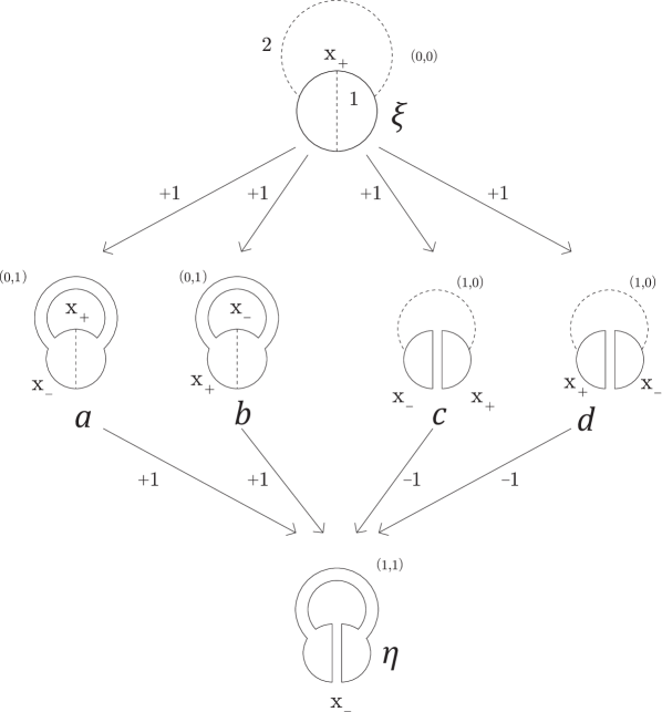
Figure 15. The poset for the decorated resolution configuration associated with a ladybug configuration in $S^{2}$

3.3. Ladybug and quasi-ladybug configurations for link diagrams in surfaces

Definition 3.13.

([11]) Let $D$ be a resolution configuration which is made of one circle and two m-arcs (multiplication arc).

Stand at a point in the circle where you see an arc to your right. Go ahead along the circle. Go around one time. Assume that you encounter the following pattern: In the order of travel you next touch the other arc. Then you touch the first arc. Then you touch the other arc again. Finally, you come back to the point at the beginning.

Since both arcs are m-arcs, both satisfy the following property: At both endpoints of each arc, you see the arc in the same side – either on the right hand side and on the left hand side.

If you see the arcs both in the right hand side and in the left hand side (respectively, only in the right hand side) while you go around one time, we call $D$ a ladybug configuration (respectively, quasi-ladybug configuration).

If $F$ is the 2-sphere, our definition of ladybug configurations is the same as that in in §3.2.1.

Let $D$ be a ladybug (respectively, quasi-ladybug) configuration. Then $Z(D)$ have only one circle and $A(D)$ have only two arcs. Make $s(D)$. Give $D$ (respectively, $s(D)$) a labeling $x$ (respectively, $y$). We call the decorated resolution configuration $(D,y,x)$ a decorated resolution configuration associated with the ladybug $($respectively, quasi-ladybug$)$ configuration $D$.

Note that $(D,y,x)$ may be empty as explained below.

Since each of $D$ and $s(D)$ has only one circle, we can let $x_{+}$ or $x_{-}$ denote $x$ (respectively, $y$).

See Figure 16.

The partial order defined in [17, Definition 2.10] is defined in the case of link diagrams in $S^{2}$. The authors [11] generalized it to the case of links in thickened surfaces.

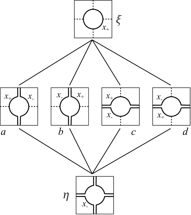
Figure 16. The poset for a decorated resolution configuration $(D,x_{-},x_{+})$ associated with a quasi-ladybug configuration on $T^{2}$: We envelope $T^{2}$ along two circles as usual, and draw six labeled resolution configurations. Here, we have $[\xi;a]\cdot[a;\eta]=[\xi;b]\cdot[b;\eta]=-[\xi;c]\cdot[c;\eta]=-[\xi;d]\cdot[d;\eta].$

Proposition 3.14.

([11]) $(1)$ Let $D$ be a quasi-ladybug configuration in a surface $F$. Assume that the only one circle in $D$ is contractible. Let $F$ be the torus. Then there is a non-vacuous decorated resolution configuration $(D,x_{-},x_{+})$ associated with $D$.

$(2)$ Let $D$ be a quasi-ladybug configuration in a surface $F$. Assume that the only one circle in $D$ is contractible. Let $(D,y,x)$ be a decorated resolution configuration associated with $D$. Assume that the genus of $F$ is greater than one. Then $(D,y,x)$ is empty for arbitrary $x$ and $y$.

$(3)$ Let $D$ be a ladybug $($respectively, quasi-ladybug$)$ configuration in a surface $F$. Let $(D,y,x)$ be a decorated resolution configuration associated with $D$. Assume that the only one circle in $D$ is non-contractible. Then $(D,y,x)$ is empty for arbitrary $x$ and $y$.

$(4)$ Let $F$ be an arbitrary surface. There is a ladybug configuration $D$ in $F$ such that a decorated resolution configuration $(D,y,x)$ associated with $D$ is non-empty.

3.4. Decorated resolution configurations of index $3$

All resolution configurations with three arcs are made from graphs in Figure 17.

1

2

3

4

5

6

7

8

9

10

11

12

13

14

15

16

17

18

19

Figure 17. Connected graphs of the resolution configurations of index 3: The segments denote arcs. We do not use dotted segments here.

Most of the configurations contain a leaf or a coleaf. Hence, they can be reduced to decorated configurations of smaller index.

Using Propositions 3.6 and 3.7 we can enumerate the diagrams without leaves and coleaves, see Fig. 18.

Figure 18. Initial configurations of decorated resolutions of index $3$ with one circle and without leaves and coleaves. The labels of the circles are $x_{+}$.

The diagrams (1)–(2”) are local, i.e. can be drawn in a disk of the surface. Note that the diagrams (1) and (1’) ((2), (2’) and (2”)) are isotopic if one considers them as diagrams in the sphere $S^{2}$. Then diagrams (3)–(6) are parameterized by the homotopy class $\alpha$ of a nontrivial simple loop in the sphere. The diagrams (7)–(8) contain a pair of interlaced outer chords (quasi-ladybug configuration) and can occur only when $F=T^{2}$ is the torus.

4. Moduli spaces

In the subsequent sections we consider concrete examples of branched covering moduli systems.

4.1. Case (C) for links in surfaces

We starts with the cubic case, i.e. with moduli systems which cover trivially the moduli spaces of the cubic flow category.

We define the moduli spaces $\mathcal{M}(D,x,y)$ by induction on the index $n$ of decorated resolution configuration $(D,x,y)$.

Case $n=1$. We set $\mathcal{M}(D,x,y)\simeq\mathcal{M}_{\mathcal{C}_{C}(1)}(\bar{1},\bar{0})$ to be one point.

Case $n=2$. The moduli space $\mathcal{M}_{\mathcal{C}_{C}(2)}(\bar{1},\bar{0})$ can be identified with the segment $I=[0,1]$.

In all cases except the ladybug and quasi-ladybug configurations (see Fig. 13) there are four labeled resolution configurations in $(D,x,y)$ that correspond to the vertices of a square, i.e. the objects of $\mathcal{C}_{C}(2)$. Thus, we can identify the moduli space $\mathcal{M}(D,x,y)$ with $\mathcal{M}_{\mathcal{C}_{C}(2)}(\bar{1},\bar{0})=I$.

In a (quasi)-ladybug configuration the boundary $\partial\mathcal{M}(D,x,y)$ consists of four points $a,b,c,d$ which correspond to the paths in the diagram of the decorated resolution configuration, see Fig. 20 and 25. By induction, the points $a$ and $b$ project to one end of the segment $I$, and $c$ and $d$ project to the other end. We must extend this projection to a $2$-fold covering over $I$. There are two ways to do this, and we must choose one of them.

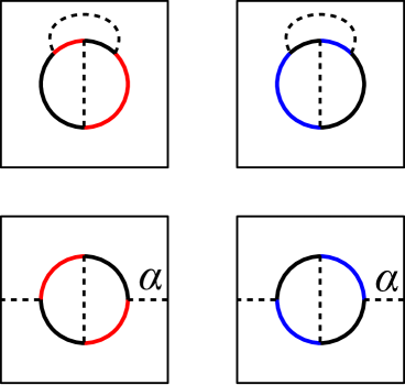
Figure 19. Right pairs (right column) and left pairs (left column) in ladybug resolution configurations

For a ladybug configuration we can use left-right pair convention from the paper [17]. The ends of the arcs splits the cycle of the decorated resolution configuration into four segments. For the right pairs, we take the segments that start in the endpoint of the arc which goes to the right, and end in the endpoint of the arc which goes to the left, see Fig. 19. The we pair the labeled resolution configurations which have the same labels on the distinguished segments of the cycle: $a$ with $d$, $b$ with $c$. The moduli space $\mathcal{M}(D,x,y)$ is the disjoint union of segments $ad$ and $bc$, see Fig. 21.

Analogously, the moduli space for the left pairs can be defined.

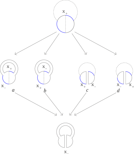
Figure 20. Decorated diagram in a ladybug case. The blue segments are the right pairs in the cycle.

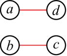
Figure 21. The moduli space in (quasi-)ladybug case

In the quasi-ladybug case, the cycle must be contractible (otherwise the decorated resolution configuration will be empty due to the homotopical grading). Then the orientation of the torus induces a canonical orientation of the cycle.

Any arc with the ends on the cycle determines a homology class in $H_{1}(T^{2},\mathbb{Z})$ (we take the class of the loop that the arc becomes after contraction the cycle to a point).

Let us define an analogue of right pairs in the quasi-ladybug case. Fix a prime element $\lambda\in H_{1}(T^{2},\mathbb{Z})$. It defines a simple curve in the torus. Choose a class $\mu$ such that $\lambda\cdot\mu=1$. Then $\lambda,\mu$ is a basis of $H_{1}(T^{2},\mathbb{Z})$.

Any arc $a$ with ends on the cycle determines a homology class in $H_{1}(T^{2},\mathbb{Z})$. Then $a=p\lambda+q\mu$, $p,q\in\mathbb{Z}$. We assign the number $-\frac{p}{q}$ to the arc $a$ (if $a=\pm\lambda$ we assign $-\infty$ to $a$). This numbering defines an order on the arcs of the decorated resolution configuration. Informally speaking, we number the arcs moving counterclockwise on the cycle, starting from an endpoint of the longitude on the cycle, see Fig. 22.

In a quasi-ladybug decorated resolution configuration we take the segments of the cycle which start at the arc with the bigger number and end at the arc the smaller number, see Fig. 22.

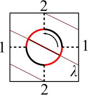
Figure 22. The $\lambda$-pair.

We shall call this pair of segments of the cycle the $\lambda$-pair. The other two segments form the $\bar{\lambda}$-pair, see Fig. 23.

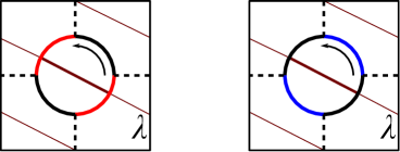
Figure 23. The $\lambda$-pairs (left) and the $\bar{\lambda}$-pairs (right).

Note that the $\lambda$-pair does not depend on the orientation of the cycle in the case when the arcs differ from $\lambda$ (as elements in $H_{1}(T^{2},\mathbb{Z})$). The segments which form the $\lambda$-pair can be thought of as the segments of the cycle (with ends at the arcs) which intersect the longitude $\lambda$. But the orientation matters when one of the arcs is homologous to $\lambda$, see Fig. 23.

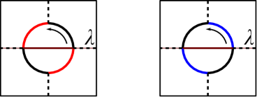
Figure 24. The $\lambda$ and $\bar{\lambda}$-pairs when one of the arcs is homologous to $\lambda$.

We pair the labeled resolution configurations which have the same labels on the distinguished segments of the cycle ($a$ with $d$, $b$ with $c$), see Fig. 25. Thus, we get the moduli space $\mathcal{M}(D,x,y)$ to be equal the disjoint union of segments $ad$ and $bc$, see Fig. 21.

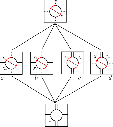
Figure 25. Decorated diagram in the quasi-ladybug case. The red segments are the $\lambda$-pairs.

Thus, in order to define the moduli spaces of index $2$ we need to fix choices $\pi(0),\pi(\alpha)\in\{l,r\}$ of left/right pairs for ladybug configurations $L_{0}$ and $L_{\alpha}$, and choices $\pi(\alpha,\beta)=\pi(\alpha,\beta)\in\{\lambda,\bar{\lambda}\}$ between $\lambda$ and $\bar{\lambda}$-pairs for quasi-ladybug configurations $Q_{\alpha,\beta}$. This set of choices $\pi$ is called a pairing.

Let $\pi_{r,\lambda}$ denote the pairing such that $\pi_{r,\lambda}(0)=r$, $\pi_{r,\lambda}(\alpha)=r$ for all $\alpha$, and $\pi_{r,\lambda}(\alpha,\beta)=\lambda$ for all $\alpha,\beta$. Analogously, one defines the pairings $\pi_{l,\lambda}$, $\pi_{r,\bar{\lambda}}$, $\pi_{l,\bar{\lambda}}$. We will call these pairings regular.

From now on, we fix some pairing $\pi$ (regular or not) and define the moduli spaces $\mathcal{M}(D,x,y)$ of index $2$ according to it.

Case $n=3$. The moduli space $\mathcal{M}_{\mathcal{C}_{C}(3)}(\bar{1},\bar{0})$ is a hexagon.

Let $(D,x,y)$ be a decorated resolution configuration of index $3$. The boundary $\partial\mathcal{M}(D,x,y)$ is defined by induction, and we need to extend it to a moduli space $\mathcal{M}(D,x,y)$ and a covering $\mathcal{M}(D,x,y)\to\mathcal{M}_{\mathcal{C}_{C}(3)}(\bar{1},\bar{0})$.

If the decorated resolution configuration does not include a (quasi)-ladybug configuration, there is a bijection between the labeled resolutions of $(D,x,y)$ and the vertices of the $3$-cube, and we set $\mathcal{M}(D,x,y)=\mathcal{M}_{\mathcal{C}_{C}(3)}(\bar{1},\bar{0})$.

If the decorated resolution configuration includes only a ladybug of type $L_{0}$, we are in the classical situation that was treated in [17]. The boundary $\partial\mathcal{M}(D,x,y)$ is (the boundary of) two hexagons which project naturally to $\partial\mathcal{M}_{\mathcal{C}_{C}(3)}(\bar{1},\bar{0})$. We extend this projection to a trivial $2$-fold covering $\mathcal{M}(D,x,y)\to\mathcal{M}_{\mathcal{C}_{C}(3)}(\bar{1},\bar{0})$.

If the decorated resolution configuration includes a ladybug of type $L_{\alpha}$, then it can not contain configurations of type $L_{0}$ or $Q_{\alpha,\beta}$ (otherwise the decorated resolution configuration is empty because of homotopical rading). Then we have the following initial labeled resolution configurations, see Fig. 18 (3)–(6). In all cases the homotopical grading does not interferes the poset structure of the decorated resolution configuration. Hence, we can treat the decorated configuration as if it were planar. Thus, the boundary $\partial\mathcal{M}(D,x,y)$ forms two hexagons as in the classical ladybug case, and the moduli space $\mathcal{M}(D,x,y)$ is defined as a trivial $2$-fold covering space over $\mathcal{M}_{\mathcal{C}_{C}(3)}(\bar{1},\bar{0})$.

Let us consider the case when the decorated resolution configuration includes a quasi-ladybug configuration, see Fig. 18 (7)–(10).

In the diagrams (7), (9), a quasi-ladybug configuration of type $L_{\alpha,\beta}$ appears twice in the decorated resolution configuration. In these two cases the homotopical grading does not impose additional restrictions to the poset structure of the decorated resolution configuration. Then we can consider the horizontal (if $\pi(\alpha,\beta)=\lambda$) or vertical (if $\pi(\alpha,\beta)=\bar{\lambda}$) arcs as inner and work with the decorated configuration as with one including ladybug configuration of type $L_{\beta}$ (or $L_{\alpha}$). Thus, the moduli space $\mathcal{M}(D,x,y)$ is a trivial $2$-fold covering over the hexagon $\mathcal{M}_{\mathcal{C}_{C}(3)}(\bar{1},\bar{0})$.

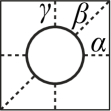
Figure 26. Initial labeled resolution configuration for the decorated configuration $DQ(\alpha,\beta,\gamma)$

Let us consider the diagram in Fig. 18 (8). Denote the homology classes of the arcs by $\alpha$, $\beta$, $\gamma$, see Fig. 26. Then the decorated resolution configuration includes three quasi-ladybug configurations of type $Q_{\alpha,\beta}$, $Q_{\beta,\gamma}$ and $Q_{\alpha,\gamma}$, see Fig. 27.

Figure 27. The decorated diagram $DQ(\alpha,\beta,\gamma)$ of index $3$

The boundary $\partial\mathcal{M}(D,x,y)$ consists of $12$ vertices which corresponds to paths from the initial to the final labeled resolution configuration in the diagram of the decorated configuration in Fig. 27. Any path is determined by the intermediate labeled configuration, for example, $1a$, $4c$ etc. An edge of $\partial\mathcal{M}(D,x,y)$ corresponds to switching between two paths with a common edge, see Fig. 28. There are six fixed edges $1a-1b$, $2a-2b$, $3a-3c$, $4a-4c$, $5b-5c$, $6b-6c$. The other six edges of $\partial\mathcal{M}(D,x,y)$ depend on the chosen pairing $\pi$.

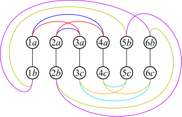
Figure 28. Pairings in $\partial\mathcal{M}(D,x,y)$. Red, orange and gold edges correspond to $\lambda$-pairs. Blue, azure and magenta labels correspond to $\bar{\lambda}$-pairs. The black edges are fixed.

Let us first consider the case when all pairs are $\lambda$-pairs: $\pi(\alpha,\beta)=\pi(\beta,\gamma)=\pi(\alpha,\gamma)=\lambda$.

Using the fixed longitude $\lambda$, we determine the $\lambda$-pairs for any pair of arcs, see Fig. 29.

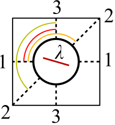
Figure 29. Segments of the $\lambda$-pairs.

We use the $\lambda$-pairs to find the moduli space of the quasi-ladybug faces. The moduli space of the face containing the labeled resolution configuration $a$ consists of segments $1a-3a$ and $2a-4a$, the other two faces give the segments $1b-5b$, $2b-6b$, $3c-5c$ and $4c-6c$. Thus, the boundary $\partial\mathcal{M}(D,x,y)$ forms two hexagons, see Fig. 30. Since the space $\partial\mathcal{M}_{\mathcal{C}_{C}(3)}(\bar{1},\bar{0})$ is a hexagon, the covering map on the boundary is trivial.

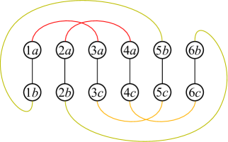
Figure 30. The boundary $\partial\mathcal{M}(D,x,y)$ of the moduli space for the $\lambda$-pairing.

Figure 31. Initial labeled resolution configuration for the decorated configuration $DQ^{\prime}(\alpha,\beta,\gamma)$. The classes $\alpha,\beta,\gamma$ are the ones of loops that appear after contracting the two cycles to points and deleting one of the three arcs.

Let us consider the diagram in Fig. 31. This decorated resolution configuration $DQ^{\prime}(\alpha,\beta,\gamma)$ (see Fig. 32) is dual to the one considered above. Thus, it has the isomorphic moduli space $\mathcal{M}(D,x,y)$: two hexagons if the number of $\bar{\lambda}$-pairings among $\pi(\alpha,\beta)$, $\pi(\beta,\gamma)$, $\pi(\alpha,\gamma)$ is even, and a dodecagon branched over the hexagon $\mathcal{M}_{\mathcal{C}_{C}(3)}(\bar{1},\bar{0})$ if the number $\bar{\lambda}$-pairings is odd.

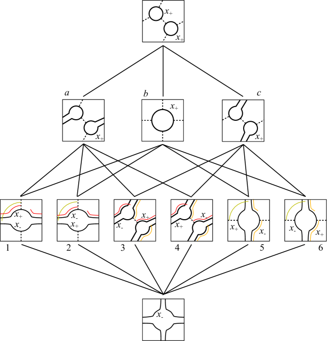
Figure 32. The decorated diagram $DQ^{\prime}(\alpha,\beta,\gamma)$ of index $3$

Thus, we see that the regular pairings $\pi_{r,\lambda}$, $\pi_{l,\lambda}$ induce trivial coverings of the moduli spaces $\mathcal{M}(D,x,y)\to\mathcal{M}_{\mathcal{C}_{C}(3)}(\bar{1},\bar{0})$ of index three. Since there is no obstruction to extension of trivial covering in higher dimensions, the moduli spaces of regular $\lambda$-pairings are trivial coverings over the cubic moduli spaces.

Thus, we have proved Theorem 2.3 for the cubic case.

4.2. Case (D) for links in surfaces

Now let us pass to the case when moduli spaces of the moduli system cover the moduli spaces of the cube flow category with branching points.

Proof of Theorem 2.3.

We construct the moduli spaces $\mathcal{M}(D,x,y)$ by induction on the index of the decorated resolution configurations. We modify moduli spaces constructed for the case (C) in the previous section.

For indices $n=1,2$ we use the moduli spaces of the cubic case. These are points ($n=1$) and one or two segments ($n=2$).

Case $n=3$. The cubic moduli spaces are one or two hexagons. For two hexagons we add a handle connecting the hexagons and make the moduli space a cylinder (Fig. 33). This space corresponds to a branched covering over the hexagon with two branch points (Fig. 34).

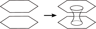
Figure 33. Branched moduli space.

Figure 34. Branching set in the moduli space of the cube flow category.

Case $n\geq 4$. Assume we have construct moduli spaces for the decorated resolution configurations of index $\leq n$. Let $(D,x,y)$ be a decorated resolution configurations of index $n$. By induction the boundary $\partial\mathcal{M}(D,x,y)$ of the moduli space is determined as a covering. This means that we have a branching submanifold of codimension 2 in the sphere $\partial\mathcal{M}_{\mathcal{C}_{C}(n)}(\bar{1},\bar{0})\simeq S^{n-2}$ such that the branched covering space is equal to

$$\partial\mathcal{M}(D,x,y)=\coprod_{(E,z)\in P(D,x,y)}\circ(\mathcal{M}(D\setminus E,z|,y|)\times\mathcal{M}(E\setminus s(D),x|,z|)).$$

The branching set $P\subset\partial\mathcal{M}_{\mathcal{C}_{C}(n)}(\bar{1},\bar{0})=S^{n-2}$ is an oriented closed $(n-4)$-dimensional manifold. Then there is a $(n-3)$-dimensional oriented manifold $Q\subset S^{n-2}$ with boundary such that $\partial Q=P$ [16, p. 50, Theorem 3]. Push the manifold $Q$ inside $B^{n-1}$ so that the deformed manifold $Q^{\prime}$ have the boundary $P=\partial Q^{\prime}=Q^{\prime}\cap S^{n-2}$ and $Q^{\prime}$ intersect the sphere $S^{n-2}$ transversely. Then we define the moduli space $\mathcal{M}(D,x,y)$ as the $2$-fold branched covering over $D^{n-1}$ with the branching set $Q^{\prime}$. ∎

Remark 4.1.

The moduli spaces constructed above differ from the moduli spaces of the case (C) by framed cobordisms. Then Pontryagin–Thom construction yields the same (up to homotopy) attaching maps in the cell complex for the Khovanov homotopy type [29]. Thus, the Khovanov homotopy type for the moduli system will be the same as the Khovanov homotopy type of the case (C).

Let us construct another moduli system for links in the torus, which has some minimality properties:

• for index $3$ the branching set in the hexagon $\mathcal{M}_{\mathcal{C}_{C}(3)}$ consists of zero or one point;

• for $n\geq 4$ the branching set in $\mathcal{M}_{\mathcal{C}_{C}(n)}$ has no components $B$ such that $B\cap\partial\mathcal{M}_{\mathcal{C}_{C}(n)}=\emptyset$.

We construct the moduli spaces $\mathcal{M}(D,x,y)$ by induction on the index of the decorated resolution configurations.

Case $n=1$. We set $\mathcal{M}(D,x,y)\simeq\mathcal{M}_{\mathcal{C}_{C}(1)}(\bar{1},\bar{0})$ to be one point.

Case $n=2$. The moduli space $\mathcal{M}_{\mathcal{C}_{C}(2)}(\bar{1},\bar{0})$ can be identified with the segment $I=[0,1]$.

In all cases except the ladybug and quasi-ladybug configurations (see Section 3.3) the multiplicity of the decorated configuration is equal to $1$, hence, there are four labeled resolution configurations in $(D,x,y)$ that correspond to the vertices of a square, i.e. the objects of $\mathcal{C}_{C}(2)$. Thus, we can identify the moduli space $\mathcal{M}(D,x,y)$ with $\mathcal{M}_{\mathcal{C}_{C}(2)}(\bar{1},\bar{0})=I$.

For ladybug and quasi-ladybug configurations (case $\mu(D,x,y)=2$) we have four points in the boundary of $\partial\mathcal{M}(D,x,y)$ which can be connected with two segments. Thus, for those configurations $\mathcal{M}(D,x,y)$ is a disjoint union two segments.

In order to define the moduli spaces of index $2$ we fix choices $\pi(0),\pi(\alpha)\in\{l,r\}$ of left/right pairs for ladybug configurations $L_{0}$ and $L_{\alpha}$, and choices $\pi(\alpha,\beta)=\pi(\alpha,\beta)\in\{\lambda,\bar{\lambda}\}$ between $\lambda$ and $\bar{\lambda}$-pairs for quasi-ladybug configurations $Q_{\alpha,\beta}$. For the (D) case we can take one of the regular pairing $\pi_{r,\bar{\lambda}}$ or $\pi_{l,\bar{\lambda}}$ (see the previous section).

Case $n=3$. The moduli space $\mathcal{M}_{\mathcal{C}_{C}(3)}(\bar{1},\bar{0})$ is a hexagon.

Let $(D,x,y)$ be a decorated resolution configuration of index $3$. The boundary $\partial\mathcal{M}(D,x,y)$ is defined by induction, and we extend it to a moduli space $\mathcal{M}(D,x,y)$ and a covering $\mathcal{M}(D,x,y)\to\mathcal{M}_{\mathcal{C}_{C}(3)}(\bar{1},\bar{0})$.

Let us show that the regular pairing $\pi_{r,\bar{\lambda}}$ gives branched moduli spaces. Consider the decorated resolution diagram $DQ(\alpha,\beta,\gamma)$ (Fig. 27).

If we use $\bar{\lambda}$-pairing: $\pi(\alpha,\beta)=\pi(\beta,\gamma)=\pi(\alpha,\gamma)=\bar{\lambda}$, the boundary $\partial\mathcal{M}(D,x,y)$ of the moduli space is a dodecagon, see Fig. 35. Then the moduli space $\mathcal{M}(D,x,y)$ should be the interior of the dodecagon. The map $\mathcal{M}(D,x,y)\to\mathcal{M}_{\mathcal{C}_{C}(3)}(\bar{1},\bar{0})$ is a $2$-fold branched covering with one branch point in the center of the dodecagon.

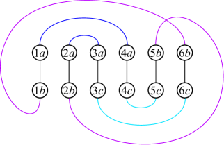
Figure 35. The boundary $\partial\mathcal{M}(D,x,y)$ of the moduli space for the $\bar{\lambda}$-pairing.

For the decorated resolution configuration $DQ^{\prime}(\alpha,\beta,\gamma)$ in Fig. 31 the $\bar{\lambda}$-pairing also gives a dodecagon moduli space.

Note that moduli spaces that covers the cubic moduli spaces with branching points can appear only for links in the torus. For this reason below we focus on the case when $F=T^{2}$.

Case $n=4$. The moduli space $\mathcal{M}_{\mathcal{C}_{C}(3)}(\bar{1},\bar{0})$ is a truncated octahedron.

Let $(D,x,y)$ be a decorated resolution configuration of index $4$. If it does not have a subconfiguration of index $3$ whose moduli space is a dodecagon, then the boundary $\partial\mathcal{M}(D,x,y)$ covers trivially the boundary $\partial\mathcal{M}_{\mathcal{C}_{C}(4)}(\bar{1},\bar{0})$. Hence, we define $\mathcal{M}(D,x,y)$ as a trivial cover over $\mathcal{M}_{\mathcal{C}_{C}(4)}(\bar{1},\bar{0})$ which is $1$ fold when $(D,x,y)$ does not include (quasi)ladybug confgurations, $2$-fold when $(D,x,y)$ includes a (quasi)ladybug confguration, and $4$-fold when $(D,x,y)$ includes two disjoint (quasi)ladybug configurations.

Now, let $(D,x,y)$ includes a subconfiguration of index $3$ with a dodecagon moduli space. At first, consider the case when this subconfiguration is $DQ(\alpha,\beta,\gamma)$. Then there exists a labeled resolution configuration $(\hat{D},z)\in P(D,x,y)$ which contains the labeled resolution configuration of Fig. 26.

Let $A$ be the set of arcs in the decorated resolution configuration $(D,x,y)$. Then there exists a subset $A_{-}\subset A$ such that $\hat{D}=s_{A_{-}}D$. Let $A_{+}=A\setminus(A_{-}\cup\{\alpha,\beta,\gamma\})$. Since $A$ consists of four arcs, then $A\setminus\{\alpha,\beta,\gamma\}=\{\delta\}$.

Assume that $A_{-}=\{\delta\}$. We can draw $\delta$ as an arc in the resolution configuration $\hat{D}=s_{\delta}(D)$. That arc can not be an outer non-contractible arc. Otherwise, the diagram $D=s_{\delta}^{-1}(D)$ would have two nontrivial cycles with label $x_{+}$, hence the decorated resolution configuration must be empty because of homotopical grading. Then $\delta$ is an inner arc or an outer coleaf. In the latter case we can draw $\delta$ as an inner coleaf.

Assume that $A_{+}=\{\delta\}$. Then $\delta$ can not be an inner arc which interlaces with arc $\alpha$, $\beta$ or $\gamma$. Otherwise, we would have an empty decorated resolution configuration like in Fig. 36 by the homotopical grading. Thus, an inner $\delta$ is a trivial arc, so it can be drawn outside the cycle. Then $\delta$ is either outer nontrivial or outer trivial arc.

Figure 36. An empty decorated resolution configuration

Thus, we have several possibilities to draw the fourth arc in the resolution configuration, see Fig. 37.

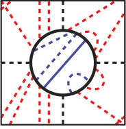
Figure 37. Possible layouts of the fourth arc in the diagram $\hat{D}$. The red arcs correspond to the cases when $\delta\in A_{+}$ and the blue arcs are cases for $\delta\in A_{-}$

.

The corresponding decorated resolution are given in Fig. 38.

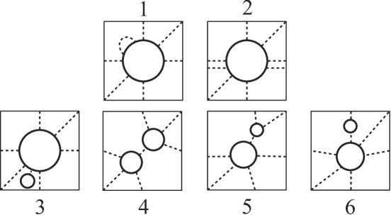
Figure 38. Decorated resolution configuration of index $4$ which includes the decorated resolution configuration $DQ(\alpha,\beta,\gamma)$.

Now, let the decorated resolution configuration $(D,x,y)$ include the subconfiguration is $DQ^{\prime}(\alpha,\beta,\gamma)$. Then there exists a labeled resolution configuration $(\hat{D},z)\in P(D,x,y)$ which contains the labeled resolution configuration of Fig. 31. Let $a$ be one of the arcs of $DQ^{\prime}(\alpha,\beta,\gamma)\subset\hat{D}$, and $\hat{D}^{\prime}=s_{a}(\hat{D})$. Then $\hat{D}^{\prime}$ has two nontrivial outer and one inner arc (which is $a$ after the surgery), see Fig. 39. We should add a fourth arc $\delta$ to those three arc. As before, we have the following restrictions:

• if $\delta\in A_{-}$ and outer then $\delta$ must be homologically trivial

• if $\delta\in A_{-}$ then it is not interlaced with $a$

• if $\delta\in A_{+}$ and inner then it is not interlaced with $\alpha$, $\beta$ or $\gamma$

This we have the following possible cases.

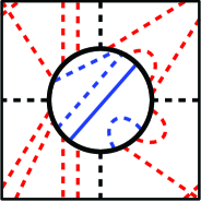
Figure 39. Possible layouts of the fourth arc in the diagram $\hat{D}^{\prime}$. The solid inner arc is the arc $a$. The red arcs correspond to the cases when $\delta\in A_{+}$ and the blue arcs are cases for $\delta\in A_{-}$

.

The corresponding decorated resolution configurations are presented in Fig. 40.

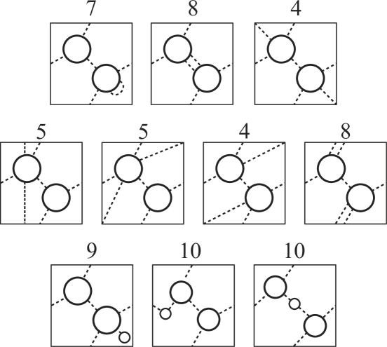
Figure 40. Decorated resolution configuration of index $4$ which includes the decorated resolution configuration $DQ^{\prime}(\alpha,\beta,\gamma)$. Same numbers correspond to isomorphic resolution configurations

Now let us describe the moduli space structure for the cases 1–10. Let $\alpha$ be the homology class of the horizontal side and $\gamma$ be the vertical side of the square which represents the torus in Fig. 38, 40. Then $\beta=\alpha+\gamma$.

The boundary $\partial\mathcal{M}(D,x,y)$ covers the surface of the moduli space $\partial\mathcal{M}_{\mathcal{C}_{C}(n)}(\bar{1},\bar{0})$. The number of $2$-faces which can have branched points (of types $DQ$ and $DQ^{\prime}$) for the cases 1–10 are given in the table.

Case	Faces of types $DQ$ and $DQ^{\prime}$
1	$2DQ(\alpha,\beta,\gamma)$
2	$2DQ(\alpha,\beta,\gamma)$
3	$2DQ(\alpha,\beta,\gamma)$
4	$2DQ(\alpha,\beta,\gamma)+2DQ(\alpha,\bar{\beta},\gamma)+2DQ^{\prime}(\alpha,\beta,\gamma)+2DQ^{\prime}(\alpha,\bar{\beta},\gamma)$
5	$DQ(\alpha,\beta,\gamma)+DQ^{\prime}(\alpha,\beta,\gamma)$
6	$2DQ(\alpha,\beta,\gamma)$
7	$2DQ^{\prime}(\alpha,\beta,\gamma)$
8	$2DQ^{\prime}(\alpha,\beta,\gamma)$
9	$2DQ^{\prime}(\alpha,\beta,\gamma)$
10	$2DQ^{\prime}(\alpha,\beta,\gamma)$

Here $\bar{\beta}=\gamma-\alpha$.

Thus, in cases 1–3,5–10, if we have $D$-case for the triple $(\alpha,\beta,\gamma)$ (i.e. the number of $\bar{\lambda}$ among the values $\pi(\alpha,\beta)$, $\pi(\alpha,\gamma)$, $\pi(\beta,\gamma)$ is odd) then the moduli space has two branched points on the boundary. The branched covering can be extended to the interior by choosing the branched set to be the segment that connects the branched points on the boundary, see Fig. 41.

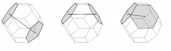
Figure 41. The branched set in the cases 1,3,7,9 (left), 2,6,8,10 (middle) and 5 (right)

The case 4 is more complicated. If there is one dodecagon triple among $(\alpha,\beta,\gamma)$ and $(\alpha,\bar{\beta},\gamma)$ then there are 4 branched points on the boundary, see Fig. 42 right. If both the triples $(\alpha,\beta,\gamma)$ and $(\alpha,\bar{\beta},\gamma)$ are in $D$-case then the number of branched points is $8$, Fig. 42 left. We can connect the branching points with two or four nonintersecting curves. Note that in this case there is no canonical way to extend the branched set from boundary to the whole moduli space.

Figure 42. Boundary branched points in the case 4

Case $n\geq 5$. Assume we have construct moduli spaces for the decorated resolution configurations of index $\leq n$. Let $(D,x,y)$ be a decorated resolution configurations of index $n$. By induction the boundary $\partial\mathcal{M}(D,x,y)$ of the moduli space is determined as a covering. This means that we have a branching submanifold of codimension 2 in the sphere $\partial\mathcal{M}_{\mathcal{C}_{C}(n)}(\bar{1},\bar{0})\simeq S^{n-2}$ such that the branched covering space is equal to

$$\partial\mathcal{M}(D,x,y)=\coprod_{(E,z)\in P(D,x,y)}\circ(\mathcal{M}(D\setminus E,z|,y|)\times\mathcal{M}(E\setminus s(D),x|,z|)).$$

The branching set $P\subset\partial\mathcal{M}_{\mathcal{C}_{C}(n)}(\bar{1},\bar{0})=S^{n-2}$ is an oriented closed $(n-4)$-dimensional manifold. Then there is a $(n-3)$-dimensional oriented manifold $Q\subset S^{n-2}$ with boundary such that $\partial Q=P$ [16, p. 50, Theorem 3]. Push the manifold $Q$ inside $B^{n-1}$ so that the deformed manifold $Q^{\prime}$ have the boundary $P=\partial Q^{\prime}=Q^{\prime}\cap S^{n-2}$ and $Q^{\prime}$ intersect the sphere $S^{n-2}$ transversely. Then we define the moduli space $\mathcal{M}(D,x,y)$ as the $2$-fold branched covering over $D^{n-1}$ with the branching set $Q^{\prime}$.

Remark 4.2.

Note that a “minimal” branching moduli systems such as considered above for links in the torus, present trivial covering (i.e. case (C)) moduli system for surfaces of other genus. Indeed, in this case quasi-ladybug configurations can not appear and for ladybug configurations any choice of left/right pairs lead to $2$-dimensional moduli spaces without branch point. Then branching sets can not appear in higher dimensions because by minimality they must intersect with the border.

4.3. Multivalued moduli systems for links in $S^{3}$

As we have seen in the previous paragraph, for links in a surface except the torus, choice of a fixed moduli space for each decorated resolution leads (under some minimality condition) to a moduli system of type (C). We can overcome this situation by considering multivalued moduli system. If we allow to choose of left/right pairs for each ladybug configuration independently then we can get moduli spaces which cover the moduli spaces of the cubic flow category with some branch point.

Consider the following example (Fig. 43). The decorated resolution configuration has index $3$ and corresponds to a 2-dimensional moduli space. The moduli space has 12 vertices which correspond to the paths from the initial to the final state in the diagram in Fig. 43. The edges of the moduli space correspond to switching between the paths by changing one of the intermediate states (Fig. 44). The decorated resolution configuration includes two ladybug configurations, so we have two choices between the left (red in the figure) and the right (blue) pairs. If we choose the left pairs for one ladybug and the right pair for the other, we get a dodecagon as the moduli space. The dodecagon covers the hexagon (the moduli space of the cubic flow category) twofold with one branch point.

Figure 43. A decorated resolution configuration with two ladybug subconfigurations

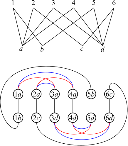
Figure 44. Boundary of the moduli space of the decorated resolution configuration

Multivalued moduli systems generalize this example.

We construct a multivalued moduli system $\mathfrak{M}$ for links in a closed oriented surface $F$ by induction on the index of the decorated resolution configurations.

Case $n=1$. Let $\mathcal{M}(D,x,y)\simeq\mathcal{M}_{\mathcal{C}_{C}(1)}(\bar{1},\bar{0})$ be the moduli space consisting of one point. We set ${\mathfrak{M}}(D,x,y)=\{\mathcal{M}(D,x,y)\}$.

Case $n=2$. The moduli space $\mathcal{M}_{\mathcal{C}_{C}(2)}(\bar{1},\bar{0})$ can be identified with the segment $I=[0,1]$.

In all cases except the ladybug and quasi-ladybug configurations the moduli space $\mathcal{M}(D,x,y)$ is identified with $\mathcal{M}_{\mathcal{C}_{C}(2)}(\bar{1},\bar{0})=I$. Then we set ${\mathfrak{M}}(D,x,y)=\{I\}$.

For ladybug and quasi-ladybug configurations (case $\mu(D,x,y)=2$) we have four points in the boundary of $\partial\mathcal{M}(D,x,y)$ which can be connected with two segments. Thus, for those configurations we have two possible moduli spaces $\mathcal{M}^{\prime}(D,x,y)$ and $\mathcal{M}^{\prime\prime}(D,x,y)$ which are disjoint unions of two segments. Then we take ${\mathfrak{M}}(D,x,y)=\{\mathcal{M}^{\prime}(D,x,y),\mathcal{M}^{\prime\prime}(D,x,y)\}$.

Case $n>2$. Let $(D,x,y)$ be a decorated resolution configurations of index $n$. By definition the boundary $\partial\mathcal{M}(D,x,y)$ must be equal to

$$\partial\mathcal{M}(D,x,y)=\coprod_{(E,z)\in P(D,x,y)}\circ(\mathcal{M}(D\setminus E,z|,y|)\times\mathcal{M}(E\setminus s(D),x|,z|)).$$

We choose all possible moduli spaces $\mathcal{M}(D\setminus E,z|,y|)\in{\mathfrak{M}}(D\setminus E,z|,y|)$, $\mathcal{M}(E\setminus s(D),x|,z|)\in{\mathfrak{M}}(E\setminus s(D),x|,z|)$ which are compatible on the boundary. After the boundary $\partial\mathcal{M}(D,x,y)$ is defined, we extend the moduli space $\mathcal{M}(D,x,y)$ as in the previous section. Then we define ${\mathfrak{M}}(D,x,y)$ as the set consisting of all possible moduli space $\mathcal{M}(D,x,y)$ constructed by this scheme.

Note that the constructed moduli spaces $\mathcal{M}(D,x,y)\in{\mathfrak{M}}(D,x,y)$ will be branch coverings over the cubic moduli spaces.

Example 4.3.

For the knot in Fig. 45 corresponding to the decorated resolution configuration in Fig. 43, we have $4$ possible variants to define moduli of index $2$. Two of these variants lead to the moduli space of index $3$ homeomorphic to two hexagons, and the other two variants yield a dodecagon. The decorated resolution configurations which are not sub-configurations of the one in Fig. 43 have multiplicity one and correspond to moduli spaces of the cube flow category. Thus, we have two potentially different Khovanov homotopy types $\mathcal{X}_{h},\mathcal{X}_{d}\in{\mathfrak{X}}_{\mathfrak{M}}(L)$ which are constructed on the hexagonal or dodecagonal moduli spaces correspondingly. But the knot is trivial, hence, its Khovanov homology is. Thus, the homotopy types coincide and ${\mathfrak{X}}_{\mathfrak{M}}(L)=\{S^{-1}\vee S^{1}\}$. This fact follows also from the invariance of the multi-valued homotopy type ${\mathfrak{X}}_{\mathfrak{M}}(L)$.

Figure 45. A diagram of the unknot

We hope to present a knot example with a nontrivial multi-valued Khovanov homotopy type in a subsequent paper.

5. The second Steenrod square operator

5.1. The first Steenrod square operator $Sq^{1}$

In [27, 28] the Steenrod square $Sq^{*}(*\in\mathbb{Z})$ is defined. Let $X$ and $X^{\prime}$ be compact CW complexes. Let $\{C_{i}\}_{i\in\mathbb{Z}}$ be a chain complex. Assume that $\{C_{i}\}_{i\in\mathbb{Z}}$ is associated with both a CW decomposition on $X$ and a CW decomposition on $X^{\prime}$. It is well-known that $Sq^{1}(X)=Sq^{1}(X^{\prime})$ (see e.g. [19, Introduction]) and that $Sq^{2}(X)$ and $Sq^{2}(X^{\prime})$ are different in general (see e.g. [26]).

Therefore, $Sq^{1}$ is not informative as a link invariant. Let us pass to $Sq^{2}$.

5.2. The second Steenrod square operator $Sq^{2}$

We review the definition of the second Steenrod square [27, 28].

Definition 5.1.

Let $K_{m}$ be the Eilenberg–MacLane space $K(\mathbb{Z}_{2},m)$ for any natural number $m>1$. By definition, $K_{m}$ is connected and $\pi_{i}(K_{m})\cong\mathbb{Z}_{2}$ (respectively, $0$) if $i=m$ (respectively, $i\neq m$ and $i\geq 1$). It is known that $H^{m+2}(K_{m};\mathbb{Z}_{2})\cong\mathbb{Z}_{2}$. Denote the generator of $H^{m+2}(K;\mathbb{Z}_{2})\cong\mathbb{Z}_{2}$ by $\xi$.

Let $X$ be a CW complex and $[X,K]$ be the set of all homotopy classes of continuous maps $X\to K$. Then $[X,K_{m}]=H^{m}(X;\mathbb{Z}_{2})$.

For an arbitrary element $x\in H^{m}(X;\mathbb{Z}_{2})$, take a continuous map $f_{x}:X\to K$ which corresponds to the class $x$. Define the second Steenrod square $Sq^{2}(x)$ of $x$ to be $f^{\ast}_{x}(\xi)\in H^{m+2}(X;\mathbb{Z}_{2})$.

This definition is reviewed and explained very well in [19, section 3.1].

We review an important property of the second Steenrod square operator $Sq^{2}$, below.

Proposition 5.2.

([27, section 12].) Let $Y$ be any compact CW complex. Let $Y^{(*)}$ be the $*$-skeleton of $Y(*\in\mathbb{Z})$. Then the second Steenrod square
$Sq^{2}(Y):H^{m}(Y;\mathbb{Z}_{2})\to H^{m+2}(Y;\mathbb{Z}_{2})$ is determined by the homotopy type of $Y^{(m+2)}/Y^{(m-1)}$.

This proposition is reviewed and explained very well in [19, section 3.1].

5.3. The second Steenrod square $\mathcal{S}q^{2}$ for links in the thickened torus in both cases (C) and (D)

Let $\mathcal{L}$ be a link in the thickened torus. We constructed stable homotopy types for $\mathcal{L}$. Of course each of stable homotopy types has the second Steenrod square.

In the case (C), make a Khovanov-Liphitzs-Sarkar stable homotopy type for a triple of $\mathcal{L}$, a degree 1 homology class $\lambda\in H_{1}(T^{2};\mathbb{Z}_{2})$ and the right-left choice. Its second Steenrod square gives an invariant of a triple of $\mathcal{L}$, a degree 1 homology class $\lambda\in H_{1}(T^{2};\mathbb{Z}_{2})$, and henceforce, gives an invariant of $\mathcal{L}$.

Note. There are infinitely many choice of degree 1 homology classes. However, when we are given two link diagrams and we compare the two, we only have to calculate the second Steenrod square in a finite cases.

In Case (D), take the set of Khovanov-Liphitzs-Sarkar stable homotopy types for a pair of $\mathcal{L}$ and the right-left choice. The set of their second Steenrod squares is an invariant of a pair of $\mathcal{L}$ and the right-left choice, and therefore, gives an invariant of $\mathcal{L}$.

Note. Our invariant, the set of Steenrod squares, is calculable.

In the case of links in $S^{3}$, in [19] Lipshitz and Sarkar showed a way to calculate $\mathcal{S}q^{2}$ by using classical link diagrams. Seed calculated the second Steenrod square for links in $S^{3}$ by making a computer program of the method in [19]. He found the following explicit pair.

Theorem 5.3.

([26]) There are links $\mathcal{J}$ and $\mathcal{J}^{\prime}$ in $S^{3}$ such that the Khovanov homologies are the same, but such that the second Steenrod squares are different.

Therefore there are links $\mathcal{J}$ and $\mathcal{J}^{\prime}$ in $S^{3}$ such that the Khovanov homologies are the same, but the Khovanov stable homotopy types are different.

It is very natural to ask the following question. Are there a pair of links in the thickened torus such that the homotopical Khovanov homologies are the same, but such that the second Steenrod squares are different?

Note that all links in $B^{3}$ are regarded as links in the thickened torus if we regard $B^{3}$ is embedded in the thickened torus. Therefore, by Theorem 2.3, Theorem 2.5 and Theorem 5.3, there are links $\mathcal{J}$ and $\mathcal{J}^{\prime}$ in the thickened torus such that the homotopical Khovanov homologies are the same (they coincide with the ordinary Khovanov homology), but such that the set of the second Steenrod squares are different.

Here, it is very natural to ask the following question. Are there a pair of links in the thickened torus which are not embedded in $B^{3}$ such that the homotopical Khovanov homologies are the same, but such that the second Steenrod squares are different? The answer is a main result. See the following proof.

Proof of Main Theorem 1.1. Let $L$ be a link in the thickened torus. Consider the moduli system $\mathcal{M}$ on the torus constructed in Section 4.1. Then ${\mathcal{X}}_{\mathcal{M}}(L)$ is a Khovanov homotopy type with cubic moduli spaces which proves Main Theorem 1.1.(1).

Then consider the moduli system $\mathcal{M}^{\prime}$ on the torus constructed in Section 4.2. The complex ${\mathcal{X}}_{\mathcal{M}^{\prime}}(L)$ is a Khovanov homotopy type with non-cubic moduli spaces which proves Main Theorem 1.1.(2).

An easy example which proves Main Theorem 1.1.(3) is given above in the page 5.3. We show a little more complicated example below, and give an alternative proof of Main Theorem 1.1.(3).

Let $C$ be a circle in $T^{2}$ which represents a nontrivial element of $H_{1}(F;\mathbb{Z})$. Regard $A$ as a knot in $F\times[-1,1]$. Take $\mathcal{J}$ and $\mathcal{J}^{\prime}$ in a 3-ball $B$ embedded in $F\times[-1,1]$, which are written in Theorem 5.3. Assume that $C\cap B=\emptyset$. Make a disjoint 2-component link which is made from $C$ and $\mathcal{J}$ (respectively, $\mathcal{J^{\prime}}$). By Theorem 5.3, these two links have different Steenrod squares and the same Khovanov homology.

See [17, §10.2] for Khovanov-Lipshitz-Sarkar stable homotopy type of disjoint links.

In this case, we do not have a quasi-ladybug configuration. The right pair and the left one of ladybug situations give the same Steenrod second square by explicit calculus which uses that about the classical link diagram $K$. (Note that the Steenrod square is only one element in this case.)

Replace $C$ with a link whose diagram is drawn in Figure 27. This example gives a case which we use a dodecagon moduli. ∎

The above example is just the beginning of many possible applications of the result in this paper. Further applications require deeper computations of the virtual Khovanov homology and will be the subject of a subsequent paper.

Louis H. Kauffman

Department of Mathematics, Statistics and Computer Science

University of Illinois at Chicago

851 South Morgan Street

Chicago, Illinois 60607-7045

USA

and

Department of Mechanics and Mathematics

Novosibirsk State University

Novosibirsk

Russia

kauffman@uic.edu

Igor Mikhailovich Nikonov

Department of Mechanics and Mathematics

Lomonosov Moscow State University

Leninskiye Gory, GSP-1

Moscow, 119991

Russia

nikonov@mech.math.msu.su

Eiji Ogasa

Meijigakuin University, Computer Science

Yokohama, Kanagawa, 244-8539

Japan

pqr100pqr100@yahoo.co.jp

ogasa@mail1.meijigkakuin.ac.jp

References

- [1] M. M. Asaeda, J. H. Przytycki, and A. S. Sikora; Categorification of the Kauffman bracket skein module of -bundles over surfaces, Algebraic & Geometric Topology 4 (2004) 1177–1210 ATG
- [2] J. A. Baldwin: On the spectral sequence from Khovanov homology to Heegaard Floer homology, Int. Math. Res. Not. 15 (2011) 3426–3470.
- [3] D. Bar-Natan: On Khovanov’s categorification of the Jones polynomial, Algebr. Geom. Topol. 2(2002), 337–370 (electronic). MR 1917056 (2003h:57014).
- [4] H. A. Dye, A. Kaestner, and L. H. Kauffman: Khovanov Homology, Lee Homology and a Rasmussen Invariant for Virtual Knots, Journal of Knot Theory and Its Ramifications 26 (2017).
- [5] W. Haken: Theorie der Normalflächen, Acta Mathematica 105 (1961) 245–375.
- [6] L. H. Kauffman: State models and the Jones polynomial, Topology 26 (1987) 395-407.
- [7] L. H. Kauffman: Talks at MSRI Meeting in January 1997, AMS Meeting at University of Maryland, College Park in March 1997, Isaac Newton Institute Lecture in November 1997, Knots in Hellas Meeting in Delphi, Greece in July 1998, APCTP-NANKAI Symposium on Yang-Baxter Systems, Non-Linear Models and Applications at Seoul, Korea in October 1998
- [8] L. H. Kauffman: Virtual Knot Theory, Europ. J. Combinatorics (1999) 20, 663–691, Article No. eujc.1999.0314, Available online at http://www.idealibrary.com math/9811028 [math.GT].
- [9] L. H. Kauffman: Introduction to virtual knot theory, J. Knot Theory Ramifications 21 (2012), no. 13, 1240007, 37 pp.
- [10] L. H. Kauffman and W.D. Neumann: Products of knots, branched fibrations and sums of singulatities, Topology 16 (1977), pp. 369–393.
- [11] L. H. Kauffman, I. M. Nikonov, and E. Ogasa: Khovanov-Lipshitz-Sarkar homotopy type for links in thickened higher genus surfaces arXiv: 2007.09241[math.GT].
- [12] L. H. Kauffman and E. Ogasa: Steenrod square for virtual links toward Khovanov-Lipshitz-Sarkar stable homotopy type for virtual links, arXiv:2001.07789 [math.GT].
- [13] M. Khovanov: A categorification of the Jones polynomial, Duke Math. J. 101 (2000), no. 3, 359–426. MR 1740682 (2002j:57025).
- [14] P. B. Kronheimer and T. S. Mrowka: Khovanov homology is an unknot-detector, Publications mathématiques de l’IHÉS 113 (2011) 97–208.
- [15] G. Kuperberg: What is a virtual link? Algebr. Geom. Topol. 3 (2003) 587-591.
- [16] R. Kirby, Topology of manifolds, Springer, 1980
- [17] R. Lipshitz and S. Sarkar: A Khovanov stable homotopy type, J. Amer. Math. Soc. 27 (2014), no. 4, 983–1042. MR 3230817
- [18] R. Lipshitz and S. Sarkar: A refinement of Rasmussen’s s-invariant, Duke Math. J. 163 (2014), no. 5, 923–952. MR 3189434
- [19] R. Lipshitz and S. Sarkar: A Steenrod square on Khovanov homology, J. Topol. 7 (2014), no. 3, 817–848. MR 3252965
- [20] V O Manturov: Khovanov homology for virtual links with arbitrary coeficients, Journal of Knot Theory and Its Ramifications 16 (2007).
- [21] V. O. Manturov and I. M. Nikonov: Homotopical Khovanov homology, Journal of Knot Theory and Its Ramifications 24 (2015) 1541003.
- [22] P. S. Ozsváth and Z. Szabó: Holomorphic disks and genus bounds, Geom. Topol. Volume 8, Number 1 (2004), 311-334.
- [23] J. Rasmussen: Khovanov homology and the slice genus, Inventiones mathematicae 182 (2010) 419–447.
- [24] N. Reshetikhin and V. G. Turaev: Invariants of 3-manifolds via link polynomials and quantum groups, Inventiones mathematicae 103 (1991) 547–597.
- [25] W. Rushworth: Doubled Khovanov Homology, Can. j. math. 70 (2018) 1130-1172.
- [26] C. Seed: Computations of the Lipshitz-Sarkar Steenrod square on Khovanov homology, arXiv:1210.1882.
- [27] N. E. Steenrod: Cohomology operations, and obstructionsto extending continuous functions, Advances in Math. 8 (1972) 371-416.
- [28] N. E. Steenrod (Author) and D. B. A. Epstein (Editor): Cohomology Operations, Annals of Mathematics Studies, Princeton University Press (1962).
- [29] R. E. Stong: Notes on Cobordism Theory, Princeton University Press (1968).
- [30] D. Tubbenhauer: Virtual Khovanov homology using cobordisms, J. Knot Theory Ramifications 23 (2014), no. 9, 1450046, 91 pp.
- [31] E. Witten: Quantum field theory and the Jones polynomial, Comm. Math. Phys. 121 (1989) 351-399.