Renormalisation of the two-dimensional border-collision normal form.

Abstract

We study the two-dimensional border-collision normal form (a four-parameter family of continuous, piecewise-linear maps on $\mathbb{R}^{2}$) in the robust chaos parameter region of [S. Banerjee, J.A. Yorke, C. Grebogi, Robust Chaos, Phys. Rev. Lett. 80(14):3049–3052, 1998]. We use renormalisation to partition this region by the number of connected components of a chaotic Milnor attractor. This reveals previously undescribed bifurcation structure in a succinct way.

1 Introduction

Piecewise-linear maps can exhibit complicated dynamics yet are relatively amenable to an exact analysis. For this reason they provide a useful tool for us to explore complex aspects of dynamical systems, such as chaos. They arise as approximations to certain types of grazing bifurcations of piecewise-smooth ODE systems [5], and are used as mathematical models, particularly in social sciences [21].

In this paper we study the family of maps

$$(x,y)\mapsto f_{\xi}(x,y)=\begin{cases}\begin{bmatrix}\tau_{L}x+y+1\\ -\delta_{L}x\end{bmatrix},&x\leq 0,\\ \begin{bmatrix}\tau_{R}x+y+1\\ -\delta_{R}x\end{bmatrix},&x\geq 0,\end{cases}$$ (1.1)

where

$$\xi=\mathopen{}\mathclose{{}\left(\tau_{L},\delta_{L},\tau_{R},\delta_{R}}\right).$$ (1.2)

With $(x,y)\in\mathbb{R}^{2}$ and $\xi\in\mathbb{R}^{4}$, this is the two-dimensional border-collision normal form [17], except the border-collision bifurcation parameter (often denoted $\mu$) has been scaled to $1$. It is a normal form in the sense that any continuous, piecewise-linear map with two pieces for which the image of the switching line intersects the switching line at a unique point that is not a fixed point, can be transformed to (1.1) under an affine change of coordinates, see for instance [26]. With $\tau_{R}=-\tau_{L}$ and $\delta_{L}=\delta_{R}$, (1.1) reduces to the well-studied Lozi map [12].

While (1.1) appears simple its dynamics can be remarkably rich [1, 6, 23, 27, 29]. In [2] Banerjee, Yorke, and Grebogi identified an open parameter region $\Phi_{\rm BYG}\subset\mathbb{R}^{4}$ (defined below) throughout which $f_{\xi}$ has a chaotic attractor, and this was shown formally in [8]. Their work popularised the notion that families of piecewise-linear maps typically exhibit chaos in a robust fashion. This is distinct from families of one-dimensional unimodal maps — often promoted as a paradigm for chaos — that have dense windows of periodicity [9, 13]. Robust chaos had already been demonstrated by Misiurewicz in the Lozi map [16], but by studying the border-collision normal form, Banerjee, Yorke, and Grebogi showed that robust chaos occurs for generic families of piecewise-linear maps.

However, while $f_{\xi}$ has a chaotic attractor for all $\xi\in\Phi_{\rm BYG}$, the attractor undergoes bifurcations, or crises [10], as the value of $\xi$ is varied within $\Phi_{\rm BYG}$. The purpose of this paper is to reveal bifurcation structure within $\Phi_{\rm BYG}$ and we achieve this via renormalisation.

Broadly speaking, renormalisation involves showing that, for some member of a family of maps, a higher iterate or induced map is conjugate to a different member of this family [14]. By employing this relationship recursively one can obtain far-reaching results. Renormalisation is central for understanding generic families of one-dimensional maps [3, 4]. For instance, Feigenbaum’s constant ($4.6692\ldots$) for the scaling of period-doubling cascades is the eigenvalue with largest modulus of a fixed point of a renormalisation operator for unimodal maps.

For the one-dimensional analogue of (1.1) (skew tent maps) the bifurcation structure was determined by Ito et. al. [11] via renormalisation, see also [28]. More recently renormalisation was applied to a two-parameter family of two-dimensional, piecewise-linear maps in [19, 20]. Their results show that for any $n\geq 1$ there exists $\xi\in\mathbb{R}^{4}$ such that (1.1) has $2^{n}$ coexisting chaotic attractors.

We apply renormalisation to (1.1) in the following way. On the preimage of the closed right half-plane, denoted $\Pi_{\xi}$, the second iterate of $f_{\xi}$ is conjugate to an alternate member of (1.1). That is, $f_{\xi}^{2}$ is conjugate to $f_{g(\xi)}$ for a certain function $g:\mathbb{R}^{4}\to\mathbb{R}^{4}$. By repeatedly iterating a boundary of $\Phi_{\rm BYG}$ backwards under $g$, we are able to divide $\Phi_{\rm BYG}$ into regions $\mathcal{R}_{n}$, for $n=0,1,2,\ldots$, where $f_{\xi}$ has a chaotic Milnor attractor with $2^{n}$ connected components. The regions converge to a fixed point of $g$ as $n\to\infty$. The main difficulties we overcome are in analysing the global dynamics of the nonlinear map $g$ and showing that the relevant dynamics of $f_{\xi}$ occurs entirely within $\Pi_{\xi}$.

Our main results are presented in §2, see Theorems 2.14–2.3. Sections 3–8 work toward proofs of these results. First §3 describes the phase space of (1.1), primarily saddle fixed points and their stable and unstable manifolds. Then in §4 we consider the second iterate $f_{\xi}^{2}$ on $\Pi_{\xi}$ and construct a conjugacy to $f_{g(\xi)}$. In §5 we derive geometric properties of the boundaries of $\mathcal{R}_{0}$ and in §6 study the dynamics of $g$.

Chaos is proved in the sense of a positive Lyapunov exponent. This positivity is achieved for all points in the attractor, including points whose forward orbits intersect the switching line where $f_{\xi}$ is not differentiable. This is achieved by using one-sided directional derivatives which are always well-defined in our setting, §7. A recursive application of the renormalisation is performed in §8. Finally §9 provides a discussion and outlook for future studies.

2 Main results

In this section we motivate and define the parameter region $\Phi_{\rm BYG}$ and the renormalisation operator $f_{\xi}\mapsto f_{g(\xi)}$, then state the main results. First Theorem 2.14 clarifies the geometry of the regions $\mathcal{R}_{n}\subset\mathbb{R}^{4}$. Next Theorem 2.2 informs us of the dynamics of $f_{\xi}$ in $\mathcal{R}_{0}$. Finally Theorem 2.3 describes the dynamics with $\xi\in\mathcal{R}_{n}$ and any value $n\geq 0$ and follows from a recursive application of the renormalisation to Theorem 2.2. Throughout the paper we write

$$f_{L,\xi}(x,y) =\begin{bmatrix}\tau_{L}x+y+1\\ -\delta_{L}x\end{bmatrix}, f_{R,\xi}(x,y) =\begin{bmatrix}\tau_{R}x+y+1\\ -\delta_{R}x\end{bmatrix},$$ (2.1)

for the left and right pieces of (1.1).

2.1 Two saddle fixed points

Consider the parameter region

$$\Phi=\mathopen{}\mathclose{{}\left\{\xi\in\mathbb{R}^{4}\,\big{|}\,\tau_{L}>\delta_{L}+1,\,\delta_{L}>0,\,\tau_{R}<-(\delta_{R}+1),\,\delta_{R}>0}\right\}.$$ (2.2)

For any $\xi\in\Phi$, $f_{\xi}$ has exactly two fixed points. Specifically

$$Y=\mathopen{}\mathclose{{}\left(\frac{-1}{\tau_{L}-\delta_{L}-1},\frac{\delta_{L}}{\tau_{L}-\delta_{L}-1}}\right)$$ (2.3)

is a fixed point of $f_{L,\xi}$ and lies in the left half-plane, while

$$X=\mathopen{}\mathclose{{}\left(\frac{-1}{\tau_{R}-\delta_{R}-1},\frac{\delta_{R}}{\tau_{R}-\delta_{R}-1}}\right)$$ (2.4)

is a fixed point of $f_{R,\xi}$ and lies in the right half-plane.

The eigenvalues associated with these points are those of the Jacobian matrices of $f_{L,\xi}$ and $f_{R,\xi}$:

$$A_{L}(\xi) =\begin{bmatrix}\tau_{L}&1\\ -\delta_{L}&0\end{bmatrix}, A_{R}(\xi) =\begin{bmatrix}\tau_{R}&1\\ -\delta_{R}&0\end{bmatrix}.$$ (2.5)

Notice $\tau_{L}$ and $\delta_{L}$ are the trace and determinant of $A_{L}$; similarly $\tau_{R}$ and $\delta_{R}$ are the trace and determinant of $A_{R}$. It follows that $\Phi$ is the set of all parameter combinations for which $Y$ is a saddle with positive eigenvalues and $X$ is a saddle with negative eigenvalues.

2.2 The parameter region $\Phi_{\rm BYG}$

For any $\xi\in\Phi$, $X$ and $Y$ have one-dimensional stable and unstable manifolds. Fig. 1 illustrates the stable (blue) and unstable (red) manifolds of $Y$. These intersect if and only if $\phi(\xi)\leq 0$, where

$$\phi(\xi)=\delta_{R}-(1+\tau_{R})\delta_{L}+\frac{1}{2}\big{(}(1+\tau_{R})\tau_{L}-\tau_{R}-\delta_{L}-\delta_{R}\big{)}\mathopen{}\mathclose{{}\left(\tau_{L}+\sqrt{\tau_{L}^{2}-4\delta_{L}}}\right).$$ (2.6)

Equation (2.6) can be derived by directly calculating the first few linear segments of the stable and unstable manifolds of $Y$ as they emanate from $Y$, see [8]. As a bifurcation, $\phi(\xi)=0$ is a homoclinic corner [25] and is analogous to a ‘first’ homoclinic tangency for smooth maps [18]. Banerjee, Yorke, and Grebogi [2] observed that an attractor is often destroyed here, so focussed their attention on the parameter region

$$\Phi_{\rm BYG}=\mathopen{}\mathclose{{}\left\{\xi\in\Phi\,\big{|}\,\phi(\xi)>0}\right\},$$ (2.7)

where the stable and unstable manifolds of $Y$ do not intersect. Indeed for all $\xi\in\Phi_{\rm BYG}$, $f_{\xi}$ has a trapping region and therefore a topological attractor [7].

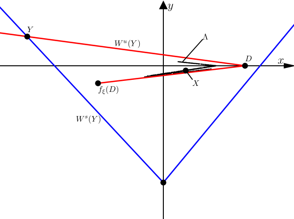
Figure 1: A sketch of the phase space of $f_{\xi}$ (1.1) with $\xi\in\Phi_{\rm BYG}$. We have shown the fixed points $X$ and $Y$ and the initial parts of $W^{s}(Y)$ (blue) and $W^{u}(Y)$ (red) as they emanate from $Y$ (these manifolds do not intersect when $\phi(\xi)>0$). The small black dots show $1000$ iterates of the forward orbit of the origin after transient dynamics has decayed.

2.3 The renormalisation operator

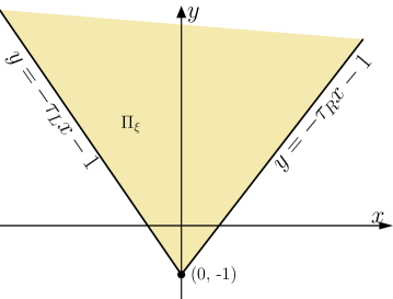
Figure 2: The preimage of the closed right half-plane (2.8).

On $\mathbb{R}^{2}$ the second iterate $f_{\xi}^{2}$ is a continuous, piecewise-linear map with four pieces. But if we restrict our attention to the set

$$\Pi_{\xi}=\mathopen{}\mathclose{{}\left\{f_{\xi}^{-1}(x,y)\,\middle|\,x\geq 0}\right\},$$ (2.8)

then $f_{\xi}^{2}$ has only two pieces:

$$f_{\xi}^{2}(x,y)=\begin{cases}\mathopen{}\mathclose{{}\left(f_{R,\xi}\circ f_{L,\xi}}\right)(x,y),&x\leq 0,\\ f_{R,\xi}^{2}(x,y),&x\geq 0.\end{cases}$$ (2.9)

As shown in Fig. 2, the boundary of $\Pi_{\xi}$ intersects the switching line at $(x,y)=(0,-1)$ and has slope $-\tau_{L}<0$ in $x<0$ and slope $-\tau_{R}>0$ in $x>0$. For any $\xi\in\Phi$, the map (2.9) is affinely conjugate to the normal form (1.1) (see Proposition 4.1). This is because the switching line of (2.9) satisfies the non-degeneracy conditions mentioned in §1.

When the affine transformation to the normal form is applied, the matrix parts of the pieces of (2.9) undergo a similarity transform, thus their traces and determinants are not changed. The matrix part of the $x\leq 0$ piece of (2.9) is $A_{R}(\xi)A_{L}(\xi)$, which has trace $\tau_{L}\tau_{R}-\delta_{L}-\delta_{R}$ and determinant $\delta_{L}\delta_{R}$. The matrix part of the $x\geq 0$ piece of (2.9) is $A_{R}(\xi)^{2}$, which has trace $\tau_{R}^{2}-2\delta_{R}$ and determinant $\delta_{R}^{2}$. Hence (2.9) can be transformed to $f_{g(\xi)}$ where

$$g(\xi)=\big{(}\tau_{R}^{2}-2\delta_{R},\delta_{R}^{2},\tau_{L}\tau_{R}-\delta_{L}-\delta_{R},\delta_{L}\delta_{R}\big{)}.$$ (2.10)

Notice we are transforming the left piece of (2.9) to the right piece of $f_{g(\xi)}$ and the right piece of (2.9) to the left piece of $f_{g(\xi)}$. This ensures $g(\xi)\in\Phi$ (see Proposition 6.1) so our renormalisation operator $f_{\xi}\mapsto f_{g(\xi)}$ produces another member of the family (1.1) in $\Phi$. Also observe

$$\xi^{*}=(1,0,-1,0)$$ (2.11)

is a fixed point of $g$ and lies on the boundary of $\Phi$.

2.4 Division of parameter space

For all $n\geq 0$ let

$$\zeta_{n}(\xi)=\phi\big{(}g^{n}(\xi)\big{)}.$$ (2.12)

The surface $\zeta_{n}(\xi)=0$ is an $n^{\rm th}$ preimage of $\phi(\xi)=0$ under $g$. We now use these surfaces to form the regions

$$\mathcal{R}_{n}=\mathopen{}\mathclose{{}\left\{\xi\in\Phi\,\big{|}\,\zeta_{n}(\xi)>0,\zeta_{n+1}(\xi)\leq 0}\right\},$$ (2.13)

for all $n\geq 0$. The following result (proved in §6.2) gives properties of these regions.

Theorem 2.1.

The $\mathcal{R}_{n}$ are non-empty, mutually disjoint, and converge to $\{\xi^{*}\}$ as $n\to\infty$. Moreover,

$$\Phi_{\rm BYG}\subset\bigcup_{n=0}^{\infty}\mathcal{R}_{n}\,.$$ (2.14)

Being four-dimensional the $\mathcal{R}_{n}$ are inherently difficult to visualise. Fig. 3 shows two-dimensional cross-sections obtained by fixing the values of $\delta_{L}>0$ and $\delta_{R}>0$. For any such cross-section only finitely many $\mathcal{R}_{n}$ are visible because as $n\to\infty$ they converge to $\{\xi^{*}\}$ for which $\delta_{L}=\delta_{R}=0$. Notice $\mathcal{R}_{1}$ contains some points that do not belong to $\Phi_{\rm BYG}$. For this reason the two sets in (2.14) are not equal.

Figure 3: Two-dimensional cross-sections of the parameter regions $\mathcal{R}_{n}$. In panel (a) $\mathcal{R}_{n}$ is visible for all $n=0,1,\ldots,4$; in panel (b) only $\mathcal{R}_{0}$ and $\mathcal{R}_{1}$ are visible. In both panels $\Phi_{\rm BYG}$ is the bounded by the vertical line $\tau_{L}=\delta_{L}+1$, the horizontal line $\tau_{R}=-\delta_{R}-1$, and the curve $\zeta_{0}=0$.

2.5 A chaotic attractor with one connected component

The next result shows $f_{\xi}$ has a chaotic, connected Milnor attractor for all $\xi\in\mathcal{R}_{0}$ when $\delta_{R}<1$. This is proved in §7.3 and based on the results of [8]. The attractor is the closure of the unstable manifold of $X$,

$$\Lambda(\xi)={\rm cl}(W^{u}(X)).$$ (2.15)

Theorem 2.2.

For the map $f_{\xi}$ with any $\xi\in\mathcal{R}_{0}$,

1. $\Lambda(\xi)$ is bounded, connected, and invariant,

2. every $z\in\Lambda(\xi)$ has a positive Lyapunov exponent, and

3. if $\delta_{R}<1$ there exists forward invariant $\Delta\subset\mathbb{R}^{2}$ with non-empty interior such that

   $$\bigcap_{n=0}^{\infty}f_{\xi}^{n}(\Delta)=\Lambda(\xi).$$ (2.16)

Lyapunov exponents for (1.1) are clarified in §7. Stronger notions of chaos have been obtained on subsets of $\mathcal{R}_{0}$, see [7, 8]. While we have not been able to prove that $\Lambda(\xi)$ is a topological attractor, (2.16) shows it contains the $\omega$-limit set of all points in $\Delta$. The set $\Delta$ has positive Lebesgue measure, thus $\Lambda(\xi)$ is a Milnor attractor [15]. If $\Delta$ is a trapping region (i.e. it maps to its interior) then $\Lambda(\xi)$ is an attracting set by definition [22]. If $\Delta$ is the trapping region of [8] (there denoted $\Omega_{\rm trap}$) then (2.16) appears to be true for some but not all $\xi\in\mathcal{R}_{0}$. We expect the extra condition $\delta_{R}<1$ is unnecessary but is included in Theorem 2.2 because our proof utilises an area-contraction argument.

2.6 A chaotic attractor with many connected components

For any $\xi\in\mathcal{R}_{n}$ we have $g^{n}(\xi)\in\mathcal{R}_{0}$ (see Lemma 6.4), while Theorem 2.2 describes the dynamics in $\mathcal{R}_{0}$. Thus by combining the renormalisation with Theorem 2.2 we are able to describe the dynamics of $f_{\xi}$ with $\xi\in\mathcal{R}_{n}$.

In view of the way $g$ is constructed, our renormalisation corresponds to the substitution rule

$$(L,R)\mapsto(RR,LR).$$ (2.17)

The same rule arises in the one-dimensional setting of Ito et. al. [11]. Given a word $\mathcal{W}$ comprised of $L$’s and $R$’s of length $k$, let $\mathcal{F}(\mathcal{W})$ be the word of length $2k$ that results from applying (2.17) to every letter in $\mathcal{W}$. If an orbit of $f_{g(\xi)}$ has symbolic itinerary $\mathcal{W}$, the corresponding orbit of $f_{\xi}$ has symbolic itinerary $\mathcal{F}(\mathcal{W})$.

The attractor of Theorem 2.2 is the closure of the unstable manifold of $X$. Consequently for $\xi\in\mathcal{R}_{n}$ the corresponding attractor is the closure of the unstable manifold of a periodic solution with symbolic itinerary $\mathcal{F}^{n}(R)$, see Table 1.

$n$	$\mathcal{F}^{n}(R)$
$0$	R
$1$	LR
$2$	RRLR
$3$	LRLRRRLR
$4$	RRLRRRLRLRLRRRLR

Table 1: The first few words in the sequence generated by repeatedly applying the symbolic substitution rule (2.17) to $R$.

Theorem 2.3.

Let $n\geq 0$ and $\xi\in\mathcal{R}_{n}$. Then $g^{n}(\xi)\in\mathcal{R}_{0}$ and there exist mutually disjoint sets $S_{0},S_{1},\ldots,S_{2^{n}-1}\subset\mathbb{R}^{2}$ such that $f_{\xi}(S_{i})=S_{(i+1)\,{\rm mod}\,2^{n}}$ and

$$f_{\xi}^{2^{n}}\big{|}_{S_{i}}~{}\text{is affinely conjugate to}~{}f_{g^{n}(\xi)}\big{|}_{\Lambda(g^{n}(\xi))}$$ (2.18)

for each $i\in\{0,1,\ldots,2^{n}-1\}$. Moreover,

$$\bigcup_{i=0}^{2^{n}-1}S_{i}={\rm cl}\mathopen{}\mathclose{{}\left(W^{u}\mathopen{}\mathclose{{}\left(\gamma_{n}}\right)}\right),$$ (2.19)

where $\gamma_{n}$ is a saddle-type periodic solution of $f_{\xi}$ with symbolic itinerary $\mathcal{F}^{n}(R)$.

Numerical explorations suggest that (2.19) is the unique attractor of (1.1) for any $\xi\in\mathcal{R}_{n}$. Theorem 2.3 tells us it has $2^{n}$ connected components and is the closure of the unstable manifold of a saddle-type period-$2^{n}$ solution. Each component $S_{i}$ is invariant under $2^{n}$ iterations of $f_{\xi}$. Equation (2.18) tells us that the dynamics of $f_{\xi}^{2^{n}}$ on $S_{i}$ is equivalent (under an affine coordinate change) to that of $f_{g^{n}(\xi)}$ on $\Lambda(g^{n}(\xi))$. Since $g^{n}(\xi)\in\mathcal{R}_{0}$, the properties listed in Theorem 2.2 apply to $f_{\xi}^{2^{n}}$ on $S_{i}$. Thus (2.19) is a chaotic Milnor attractor of $f_{\xi}$.

As an example, consider $f_{\xi}$ with

$$\xi_{\rm ex}=(1.15,0.01,-1.12,0.01)\in\mathcal{R}_{2}\,.$$ (2.20)

Fig. 4-a shows $1000$ points of the forward orbit of the origin after transient behaviour has decayed. As expected these points appear to converge to a chaotic attractor with four connected components. By Theorem 2.3 each component is affinely conjugate to $\Lambda(g^{2}(\xi))$ which is approximated in Fig. 4-b by again iterating the origin. The set $\Lambda(g^{2}(\xi))$ has a complicated branched structure but this is not visible in Fig. 4-b because the determinants are extremely small.

Figure 4: Numerically computed attractors of $f_{\xi}$ with $\xi=\xi_{\rm ex}$, (2.20), in panel (a), and $\xi=g^{2}(\xi_{\rm ex})$ in panel (b). In panel (a) the four small triangles are the points of a periodic solution with symbolic itinerary $\mathcal{F}^{2}(R)=RRLR$.

3 The stable and unstable manifolds of the fixed points

In this section we discuss the stable and unstable manifolds of the saddle fixed points $X$ and $Y$. Here and throughout the paper

$$0<\lambda_{L}^{s}<1<\lambda_{L}^{u}$$ (3.1)

denote the eigenvalues of $A_{L}$, and

$$\lambda_{R}^{u}<-1<\lambda_{R}^{s}<0$$ (3.2)

denote the eigenvalues of $A_{R}$. These are functions of $\xi$ and assume $\xi\in\Phi$.

3.1 Stable and unstable manifolds of piecewise-linear maps

Let $P$ be one of the saddle fixed points $X$ or $Y$. The stable manifold of $P$ is defined as

$$W^{s}(P)=\mathopen{}\mathclose{{}\left\{z\in\mathbb{R}^{2}\setminus\{P\}\,\big{|}\,f_{\xi}^{n}(z)\to P~{}\text{as}~{}n\to\infty}\right\}.$$ (3.3)

For all $\xi\in\Phi$ the map $f_{\xi}$ is invertible so the unstable manifold of $P$ is defined analogously as

$$W^{u}(P)=\mathopen{}\mathclose{{}\left\{z\in\mathbb{R}^{2}\setminus\{P\}\,\big{|}\,f_{\xi}^{-n}(z)\to P~{}\text{as}~{}n\to\infty}\right\}.$$ (3.4)

Since $P$ is a saddle, $W^{s}(P)$ and $W^{u}(P)$ are one-dimensional. As with smooth maps, from $P$ they emanate tangent to the stable and unstable subspaces $E^{s}(P)$ and $E^{u}(P)$. These subspaces are the lines through $P$ with directions given by the eigenvectors of ${\rm D}f_{\xi}(P)$. But since $f_{\xi}$ is piecewise-linear, $W^{s}(P)$ and $W^{u}(P)$ in fact coincide with $E^{s}(P)$ and $E^{u}(P)$ in a neighbourhood of $P$. Globally they have a piecewise-linear structure: $W^{s}(P)$ has kinks on the switching line $x=0$ and on the backward orbits of these points; $W^{u}(P)$ has kinks on the image of switching line, $y=0$, and on the forward orbits of these points.

In the remainder of this section we reproduce the geometric constructions of [8] that will be needed below.

3.2 The stable and unstable manifolds of $Y$

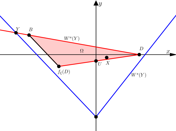
Figure 5: A sketch of the phase space of $f_{\xi}$ with $\xi\in\Phi_{\rm BYG}$. The triangle $\Omega(\xi)$ is shaded.

Since the eigenvalues of $A_{L}$ are positive, $W^{s}(Y)$ and $W^{u}(Y)$ each have two dynamically independent branches. Let $D$ denote the first kink of the right branch of $W^{u}(Y)$ as we follow it outwards from $Y$, see Fig. 5. Notice $D$ is the intersection of $E^{u}(Y)$ with $y=0$. Now let $B$ denote the intersection of $E^{u}(Y)$ with the line through $f_{\xi}(D)$ and parallel to $E^{s}(Y)$. Then let $\Omega(\xi)$ be the closed compact triangle with vertices $D$, $f_{\xi}(D)$, and $B$.

The following result says $\Omega(\xi)$ is forward invariant under $f_{\xi}$. This was proved in [8] by direct calculations. The key observation is that $f_{\xi}(D)$ lies to the right of $E^{s}(Y)$ because $\phi(\xi)>0$.

Proposition 3.1.

For any $\xi\in\Phi_{\rm BYG}$, $f_{\xi}\mathopen{}\mathclose{{}\left(\Omega(\xi)}\right)\subset\Omega(\xi)$.

The next result tells us that the attractor of Theorem 2.2 is contained in $\Omega(\xi)$.

Lemma 3.2.

For any $\xi\in\Phi_{\rm BYG}$, $\Lambda(\xi)\subset\Omega(\xi)$.

Proof.

Since $\Omega(\xi)$ is forward invariant we only need to show $X\in\Omega(\xi)$. By direct calculations we find that the line through $D$ and $f_{\xi}(D)$ is $y=\ell(x)$ where

$$\ell(x)=\frac{\delta_{R}}{\lambda_{L}^{s}-\tau_{R}}\mathopen{}\mathclose{{}\left(x-\frac{1}{1-\lambda_{L}^{s}}}\right).$$

From (2.4) we obtain, after much simplification,

$$X_{2}-\ell(X_{1})=\frac{\delta_{R}\mathopen{}\mathclose{{}\left(\lambda_{L}^{s^{2}}-\tau_{R}\lambda_{L}^{s}+\delta_{R}}\right)}{(\delta_{R}+1-\tau_{R})\mathopen{}\mathclose{{}\left(\lambda_{L}^{s}-\tau_{R}}\right)\mathopen{}\mathclose{{}\left(1-\lambda_{L}^{s}}\right)}.$$

In view of (2.2) and (3.1), each factor in this expression is positive, thus $X$ lies above the line through $D$ and $f_{\xi}(D)$. Also $X_{1}>0$ and $X_{2}<0$, thus $X\in\Omega(\xi)$ as required. ∎

3.3 The stable and unstable manifolds of $X$

Figure 6: Sketches of phase space with $\xi\in\mathcal{R}_{0}$ in panel (a) and $\xi\in\mathcal{R}_{n}$ with $n\geq 1$ in panel (b). The set $\Delta_{0}$ in panel (a) is introduced in §7.3. The set $\Omega^{\prime}$ in panel (b) is introduced in §8.1.

Since the eigenvalues of $A_{R}$ are negative, $W^{s}(X)$ and $W^{u}(X)$ each have one dynamically independent branch. Let $T$ denote the intersection of $E^{u}(X)$ with $y=0$ and let $V$ denote the intersection of $E^{s}(X)$ with $x=0$, see Fig. 6. It is easily shown that

$$T=\mathopen{}\mathclose{{}\left(\frac{1}{1-\lambda_{R}^{s}},0}\right).$$ (3.5)

If $f_{\xi}^{2}(T)$ lies to the left of $E^{s}(X)$, as in Fig. 6-a, then $W^{s}(X)$ and $W^{u}(X)$ intersect transversely. If $f_{\xi}^{2}(T)$ lies to the right of $E^{s}(X)$, as in Fig. 6-b, then $W^{s}(X)$ and $W^{u}(X)$ have no intersection. The following result was obtained in [7] by calculating $f_{\xi}^{2}(T)$ explicitly.

Proposition 3.3.

For any $\xi\in\Phi$, $f_{\xi}^{2}(T)$ lies to the left of $E^{s}(X)$ if and only if $\psi(\xi)>0$, where

$$\psi(\xi)=(\tau_{L}\tau_{R}-\delta_{R})\lambda_{R}^{u}+\mathopen{}\mathclose{{}\left(\frac{\delta_{L}}{\delta_{R}}+\delta_{L}-1}\right)\lambda_{R}^{s}-\tau_{L}(1+\delta_{R})+\tau_{R}(1-\delta_{L}).$$ (3.6)

As a bifurcation, $\psi(\xi)=0$ is a homoclinic corner for the fixed point $X$. This is analogous to the surface $\phi(\xi)=0$ for the fixed point $Y$ as discussed in §2.2.

4 The second iterate of $f_{\xi}$

As discussed in §2.3, on $\Pi_{\xi}$ the second iterate of $f_{\xi}$ is a continuous, piecewise-linear map with two pieces, (2.9). Next in §4.1 we provide the affine transformation that converts (2.9) to the normal form (1.1). Then in §4.2 we show that the bifurcation surface $\psi(\xi)=0$ of the previous section is in fact identical to $\zeta_{1}(\xi)=\phi(g(\xi))=0$.

4.1 A transformation to the normal form

Any continuous, two-piece, piecewise-linear map on $\mathbb{R}^{2}$ for which the image of the switching line intersects the switching line at a unique point that is not a fixed point can be transformed to (1.1) under an affine coordinate transformation. The required transformation is described in the original work [17]. For the generalisation to $n$ dimensions refer to [24].

The switching line of (2.9) satisfies this condition for any $\xi\in\Phi$. As clarified by Proposition 4.1, the required coordinate transformation is

$$h_{\xi}(x,y)=\frac{1}{\tau_{R}+\delta_{R}+1}\begin{bmatrix}x\\ \delta_{R}x+\tau_{R}y-\delta_{R}\end{bmatrix}.$$ (4.1)

Proposition 4.1.

For any $\xi\in\Phi$,

$$f_{\xi}^{2}=h_{\xi}^{-1}\circ f_{g(\xi)}\circ h_{\xi}\,,$$ (4.2)

on $\Pi_{\xi}$.

Proof.

By directly composing (2.1) and (4.1) we obtain

$$h_{\xi}\circ f_{\xi}^{2}=\begin{cases}\dfrac{1}{\tau_{R}+\delta_{R}+1}\begin{bmatrix}\mathopen{}\mathclose{{}\left(\tau_{R}^{2}-\delta_{R}}\right)x+\tau_{R}y+\tau_{R}+1\\ -\delta_{R}^{2}x\end{bmatrix},&x\leq 0,\\ \dfrac{1}{\tau_{R}+\delta_{R}+1}\begin{bmatrix}\mathopen{}\mathclose{{}\left(\tau_{L}\tau_{R}-\delta_{L}}\right)x+\tau_{R}y+\tau_{R}+1\\ -\delta_{L}\delta_{R}x\end{bmatrix},&x\geq 0,\end{cases}$$

and it is readily seen that $f_{g(\xi)}\circ h_{\xi}$ produces the same expression. ∎

Write $(\tilde{x},\tilde{y})=h_{\xi}(x,y)$. Notice that $x$ and $\tilde{x}$ have opposite signs, i.e.

$${\rm sgn}(x)=-{\rm sgn}(\tilde{x}).$$ (4.3)

This is because $\tau_{R}+\delta_{R}+1<0$ by (2.2). Thus the left piece of $f_{g(\xi)}$ corresponds to the right piece of $f_{\xi}^{2}$ in (2.9), and this is consistent with how $g$ was introduced in §2.3.

4.2 A reinterpretation of $\psi$

In §3.3 we saw that the fixed point $X$ of $f_{\xi}$ has a homoclinic corner when $\psi(\xi)=0$. The same is true for $f_{\xi}^{2}$: its fixed point $X$ has a homoclinic corner when $\psi(\xi)=0$. Notice $X$ is a fixed point of $f_{R,\xi}^{2}$, which is transformed under (4.2) to $f_{L,g(\xi)}$, which has the fixed point $Y$. Thus, while the stable and unstable manifolds of $X$ lie in $\Pi_{\xi}$, they transform to the stable and unstable manifolds of $Y$ for $f_{g(\xi)}$. The latter manifolds have a homoclinic corner when $\phi(g(\xi))=0$, which suggests that $\psi(\xi)=0$ and $\phi(g(\xi))=0$ are the same surface. The following result tells us that this is indeed the case.

Lemma 4.2.

For any $\xi\in\Phi$,

$$\phi(g(\xi))=\tau_{R}\lambda_{R}^{u^{2}}\psi(\xi).$$ (4.4)

Proof.

Equation (2.6) can be written as

$$\phi(\xi)=(1+\tau_{R})\lambda_{L}^{u^{2}}-(\tau_{R}+\delta_{L}+\delta_{R})\lambda_{L}^{u}+\delta_{R}\,.$$ (4.5)

To evaluate $\phi(g(\xi))$, in (4.5) we replace $\delta_{L}$ with $\delta_{R}^{2}$, $\delta_{R}$ with $\delta_{L}\delta_{R}$, and $\tau_{R}$ with $\tau_{L}\tau_{R}-\delta_{L}-\delta_{R}$, see (2.10). Also we replace $\lambda_{L}^{u}$ with $\lambda_{R}^{u^{2}}$ because $\lambda_{R}^{u^{2}}$ is the unstable eigenvalue of $A_{R}^{2}$ (which has trace and determinant given by the first two components of (2.10)). It is a simple (though tedious) exercise to show that upon performing these substitutions and simplifying we obtain $\tau_{R}\lambda_{R}^{u^{2}}\psi(\xi)$. ∎

5 The geometry of the boundary of $\mathcal{R}_{0}$

The region $\mathcal{R}_{0}\subset\mathbb{R}^{4}$ is bounded by $\zeta_{0}(\xi)=\phi(\xi)=0$, $\zeta_{1}(\xi)=\phi(g(\xi))=0$, and the hyperplanes specified in (2.2). Since parameter space is four-dimensional these are difficult to visualise. We can benefit from the fact that the $\delta_{L}$ and $\delta_{R}$ components of $g$ are decoupled from $\tau_{L}$ and $\tau_{R}$. Thus two-dimensional slices

$$\Phi_{\rm slice}(\delta_{L},\delta_{R})=\mathopen{}\mathclose{{}\left\{(\tau_{L},\tau_{R})\,\middle|\,\tau_{L}>\delta_{L}+1,\tau_{R}<-\delta_{R}-1}\right\},$$ (5.1)

defined by fixing the values of $\delta_{L}$ and $\delta_{R}$, map to one another under $g$. In any such slice $\zeta_{0}(\xi)=0$ and $\zeta_{1}(\xi)=0$ are curves. In this section we show that for any values $0<\delta_{L}<1$ and $0<\delta_{R}<1$, these curves have the geometry shown in Fig. 7.

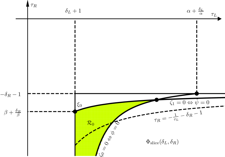
Figure 7: A sketch of $\zeta_{0}(\xi)=0$ and $\zeta_{1}(\xi)=0$ (equivalently $\phi(\xi)=0$ and $\hat{\psi}(\xi)=0$) in $\Phi_{\rm slice}(\delta_{L},\delta_{R})$ with $0<\delta_{L}<1$ and $0<\delta_{R}<1$. The curve $\tau_{R}=-\frac{1}{\tau_{L}}-\delta_{R}-1$ is shown dashed.

Observe $\zeta_{0}(\xi)=0$ is the same as $\phi(\xi)=0$, while, by Lemma 4.4, $\zeta_{1}(\xi)=0$ is the same as $\psi(\xi)=0$. However, we find the function

$$\hat{\psi}(\xi)=\lambda_{R}^{u}\psi(\xi),$$ (5.2)

easier to work with $\psi(\xi)$. By (4.4) the sign of $\hat{\psi}(\xi)$ is the same as that of $\zeta_{1}(\xi)$. From (3.6) we obtain

$$\hat{\psi}(\xi)=-\delta_{L}\mathopen{}\mathclose{{}\left(\lambda_{R}^{u^{2}}-1}\right)+\lambda_{R}^{u}\mathopen{}\mathclose{{}\left(\lambda_{R}^{u^{2}}-1}\right)\tau_{L}+(1-\delta_{R})\lambda_{R}^{u^{2}}\,.$$ (5.3)

The remainder of this section is organised as follows. First in §5.1 we study the curve $\phi(\xi)=0$. We then derive analogous properties for $\hat{\psi}(\xi)=0$ and obtain some additional bounds, §5.2. Lastly we show these curves intersect at a unique point in $\Phi_{\rm slice}$, §5.3.

5.1 The curve $\phi(\xi)=0$

We first show the curve $\phi(\xi)=0$ does not exist in $\Phi_{\rm slice}(\delta_{L},\delta_{R})$ if $\delta_{L}\geq 1$.

Lemma 5.1.

Let $\xi\in\Phi$. If $\delta_{L}\geq 1$ then $\phi(\xi)<0$.

Proof.

We can rearrange (4.5) as

$$\phi(\xi)=(\tau_{R}+\delta_{R}+1)\lambda_{L}^{u}\mathopen{}\mathclose{{}\left(\lambda_{L}^{u}-1}\right)-\delta_{R}\mathopen{}\mathclose{{}\left(\lambda_{L}^{u^{2}}-1}\right)+(1-\delta_{L})\lambda_{L}^{u}\,.$$ (5.4)

By inspection the first two terms in (5.4) are negative and if $\delta_{L}\geq 1$ then the last term is less than or equal to zero. ∎

The next result shows that $\phi(\xi)=0$ appears roughly as in Fig. 7.

Proposition 5.2.

Let $0<\delta_{L}<1$ and $\delta_{R}>0$. There exists a unique $C^{\infty}$ function $G:(-\infty,-\delta_{R}-1]\to(\delta_{L}+1,\infty)$ such that

$$\phi\big{(}G(\tau_{R}),\delta_{L},\tau_{R},\delta_{R}\big{)}=0,$$ (5.5)

for all $\tau_{R}\in(-\infty,-\delta_{R}-1]$. Moreover, $G$ is strictly increasing, $G(\tau_{R})\to\delta_{L}+1$ as $\tau_{R}\to-\infty$, and $G(-\delta_{R}-1)=\alpha+\frac{\delta_{L}}{\alpha}$ where $\alpha\in\mathbb{R}$ is the largest solution to

$$-\delta_{R}\alpha^{2}+(1-\delta_{L})\alpha+\delta_{R}=0\,.$$ (5.6)

Proof.

First fix $\tau_{R}\leq-\delta_{R}-1$. With $\tau_{L}=\delta_{L}+1$ we have $\lambda_{L}^{u}=1$ and so (4.5) simplifies to $\phi(\xi)=1-\delta_{L}>0$. As $\tau_{L}\to\infty$ we have $\lambda_{L}^{u}\to\infty$ and so $\phi(\xi)\to-\infty$ (because the $\lambda_{L}^{u^{2}}$-coefficient in (4.5) is negative). Thus by the intermediate value theorem there exists $\tau_{L}=G(\tau_{R})>\delta_{L}+1$ satisfying (5.5).

To demonstrate the uniqueness of $G$ we differentiate (4.5) to obtain

$$\frac{\partial\phi}{\partial\tau_{L}}=\mathopen{}\mathclose{{}\left(2(1+\tau_{R})\lambda_{L}^{u}-(\tau_{R}+\delta_{L}+\delta_{R})}\right)\frac{\partial\lambda_{L}^{u}}{\partial\tau_{L}}.$$ (5.7)

It is a simple exercise to show that $\frac{\partial\lambda_{L}^{u}}{\partial\tau_{L}}=\frac{\lambda_{L}^{u}}{\lambda_{L}^{u}-\lambda_{L}^{s}}$. Also if $\phi=0$ then by (4.5) we can replace $(\tau_{R}+\delta_{L}+\delta_{R})$ in (5.7) with $\frac{\delta_{R}}{\lambda_{L}^{u}}+(1+\tau_{R})\lambda_{L}^{u}$ to obtain

$$\frac{\partial\phi}{\partial\tau_{L}}\bigg{|}_{\phi=0}=\mathopen{}\mathclose{{}\left((1+\tau_{R})\lambda_{L}^{u}-\frac{\delta_{R}}{\lambda_{L}^{u}}}\right)\frac{\lambda_{L}^{u}}{\lambda_{L}^{u}-\lambda_{L}^{s}}.$$ (5.8)

By inspection $\frac{\partial\phi}{\partial\tau_{L}}\big{|}_{\phi=0}<0$. Thus $G$ is unique (because if $\phi=0$ for two distinct values of $\tau_{L}>\delta_{L}+1$ then $\frac{\partial\phi}{\partial\tau_{L}}\geq 0$ at at least one of these values).

Since $\phi(\xi)$ is $C^{\infty}$ the function $G$ is $C^{\infty}$ by the implicit function theorem. From (4.5) we obtain

$$\frac{\partial\phi}{\partial\tau_{R}}=\lambda_{L}^{u}\mathopen{}\mathclose{{}\left(\lambda_{L}^{u}-1}\right),$$ (5.9)

which is evidently positive. Thus $\frac{dG}{d\tau_{R}}=-\frac{\frac{\partial\phi}{\partial\tau_{L}}}{\frac{\partial\phi}{\partial\tau_{R}}}\Big{|}_{\phi=0}>0$, so $G$ is strictly increasing.

Also $G(\tau_{R})\to\delta_{L}+1$ as $\tau_{R}\to-\infty$ because if we fix $\tau_{L}=\delta_{L}+1+\varepsilon$, then $\phi(\xi)\to-\infty$ as $\tau_{R}\to-\infty$ for any $\varepsilon>0$. Finally, by substituting $\tau_{R}=-\delta_{R}-1$ into (4.5) we obtain

$$\phi(\xi)\big{|}_{\tau_{R}=-\delta_{R}-1}=-\delta_{R}\lambda_{L}^{u^{2}}+(1-\delta_{L})\lambda_{L}^{u}+\delta_{R}\,.$$ (5.10)

Since $\tau_{L}=\lambda_{L}^{u}+\frac{\delta_{L}}{\lambda_{L}^{u}}$ we have $G(-\delta_{R}-1)=\alpha+\frac{\delta_{L}}{\alpha}$. ∎

5.2 The curve $\hat{\psi}(\xi)=0$

The arguments presented here for $\hat{\psi}$ mirror those above for $\phi$. We first show $\hat{\psi}(\xi)=0$ does not exist in $\Phi_{\rm slice}(\delta_{L},\delta_{R})$ if $\delta_{R}\geq 1$.

Lemma 5.3.

Let $\xi\in\Phi$. If $\delta_{R}\geq 1$ then $\hat{\psi}(\xi)<0$.

Proof.

By inspection the first two terms in (5.3) are negative and if $\delta_{R}\geq 1$ then the last term is less than or equal to zero. ∎

We now show $\hat{\psi}(\xi)=0$ appears roughly as in Fig. 7.

Proposition 5.4.

Let $\delta_{L}>0$ and $0<\delta_{R}<1$. There exists a unique $C^{\infty}$ function $H:[\delta_{L}+1,\infty)\to(-\infty,-\delta_{R}-1)$ such that

$$\hat{\psi}\big{(}\tau_{L},\delta_{L},H(\tau_{L}),\delta_{R}\big{)}=0,$$ (5.11)

for all $\tau_{L}\in[\delta_{L}+1,\infty)$. Moreover, $H$ is strictly increasing, $H(\tau_{L})\to-\delta_{R}-1$ as $\tau_{L}\to\infty$, and $H(\delta_{L}+1)=\beta+\frac{\delta_{R}}{\beta}$ where $\beta\in\mathbb{R}$ is the smallest (most negative) solution to $p(\beta)=0$ where

$$p(\beta)=(1+\delta_{L})\beta^{3}+(1-\delta_{L}-\delta_{R})\beta^{2}-(1+\delta_{L})\beta+\delta_{L}\,.$$ (5.12)

Proof.

Fix $\tau_{L}\geq\delta_{L}+1$. With $\tau_{R}=-\delta_{R}-1$ we have $\lambda_{R}^{u}=-1$ and so (5.3) simplifies to $\hat{\psi}(\xi)=1-\delta_{R}>0$. Also $\hat{\psi}(\xi)\to-\infty$ as $\tau_{R}\to-\infty$, thus, by the intermediate value theorem, there exists $\tau_{R}=H(\tau_{L})<-\delta_{R}-1$ satisfying (5.11).

From (5.3),

$$\frac{\partial\hat{\psi}}{\partial\tau_{R}}=\mathopen{}\mathclose{{}\left(3\tau_{L}\lambda_{R}^{u^{2}}+2(1-\delta_{L}-\delta_{R})\lambda_{R}^{u}-\tau_{L}}\right)\frac{\lambda_{R}^{u}}{\lambda_{R}^{u}-\lambda_{R}^{s}},$$

and if $\hat{\psi}(\xi)=0$ this can be simplified to

$$\frac{\partial\hat{\psi}}{\partial\tau_{R}}\bigg{|}_{\hat{\psi}=0}=\mathopen{}\mathclose{{}\left(\tau_{L}\mathopen{}\mathclose{{}\left(1+\lambda_{R}^{u^{2}}}\right)-\frac{2\delta_{L}}{\lambda_{R}^{u}}}\right)\frac{\lambda_{R}^{u}}{\lambda_{R}^{u}-\lambda_{R}^{s}},$$ (5.13)

which is positive. Hence $H(\tau_{L})$ satisfying (5.11) is unique for all $\tau_{L}\geq\delta_{L}+1$. Moreover, $H$ is $C^{\infty}$ because $\hat{\psi}$ is $C^{\infty}$. From (5.3),

$$\frac{\partial\hat{\psi}}{\partial\tau_{L}}=\lambda_{R}^{u}\mathopen{}\mathclose{{}\left(\lambda_{R}^{u^{2}}-1}\right)<0,$$

thus $\frac{dH}{d\tau_{L}}=-\frac{\frac{\partial\hat{\psi}}{\partial\tau_{R}}}{\frac{\partial\hat{\psi}}{\partial\tau_{L}}}\Big{|}_{\hat{\psi}=0}>0$, i.e. $H$ is strictly increasing.

We have $H(\tau_{L})\to-\delta_{R}-1$ as $\tau_{L}\to\infty$ because if $\tau_{R}=-\delta_{R}-1-\varepsilon$ then $\hat{\psi}(\xi)\to-\infty$ as $\tau_{L}\to\infty$ for any $\varepsilon>0$. Finally, by substituting $\tau_{L}=\delta_{L}+1$ into (5.3) we obtain $\hat{\psi}(\xi)\big{|}_{\tau_{L}=\delta_{L}+1}=p\mathopen{}\mathclose{{}\left(\lambda_{R}^{u}}\right)$ and so $H(\delta_{L}+1)=\beta+\frac{\delta_{R}}{\beta}$ as required. ∎

Next we obtain upper bounds on the values of $\beta$ and $\beta+\frac{\delta_{R}}{\beta}$. These are the values of $\lambda_{R}^{u}$ and $\tau_{R}$ for the point at which the curve $\hat{\psi}(\xi)=0$ meets the boundary $\tau_{L}=\delta_{L}+1$, see Fig. 7.

Lemma 5.5.

Let $\delta_{L}>0$ and $0<\delta_{R}<1$. The value of $\beta$ in Proposition 5.12 satisfies $\beta>-\frac{1+\sqrt{5}}{2}$ and $\beta+\frac{\delta_{R}}{\beta}>-2$.

Proof.

The function $p$ can be rewritten as

$$p(\beta)=\delta_{L}\mathopen{}\mathclose{{}\left(\beta-1}\right)^{2}\mathopen{}\mathclose{{}\left(\beta+1}\right)-\delta_{R}\beta^{2}+\beta\mathopen{}\mathclose{{}\left(\beta^{2}+\beta-1}\right).$$ (5.14)

The first two terms of (5.14) are negative, so since $p(\beta)=0$ the last term of (5.14) must be positive. This requires $\beta>-\frac{1+\sqrt{5}}{2}$.

Also $p$ can be rewritten as

$$p(\beta)=\mathopen{}\mathclose{{}\left[(\beta+1)\mathopen{}\mathclose{{}\left(1-\frac{1}{\beta}}\right)\mathopen{}\mathclose{{}\left(1+\delta_{L}-\frac{\delta_{L}}{\beta}}\right)+(1-\delta_{R})}\right]\beta^{2}.$$

Thus $p(\beta)=0$ implies

$$-(\beta+1)=\frac{1-\delta_{R}}{\mathopen{}\mathclose{{}\left(1-\frac{1}{\beta}}\right)\mathopen{}\mathclose{{}\left(1+\delta_{L}-\frac{\delta_{L}}{\beta}}\right)}.$$ (5.15)

Since $\beta<0$ the denominator of (5.15) is greater than $1$ and so $-(\beta+1)<1-\delta_{R}$. Thus $(\beta+1)^{2}<(1-\delta_{R})^{2}$ which can be rearranged as $\beta^{2}+\delta_{R}<-2\beta-\delta_{R}(1-\delta_{R})$. Since $0<\delta_{R}<1$ this can be reduced to $\beta+\frac{\delta_{R}}{\beta}>-2$. ∎

Lastly we show that the curve $\tau_{R}=-\frac{1}{\tau_{L}}-\delta_{R}-1$ lies below $\hat{\psi}(\xi)=0$, as in Fig. 7. This result is used later in the proof of Proposition 6.3.

Lemma 5.6.

Let $\delta_{L}>0$, $0<\delta_{R}<1$, and $\tau_{L}\geq\delta_{L}+1$. Then

$$H(\tau_{L})>-\frac{1}{\tau_{L}}-\delta_{R}-1.$$ (5.16)

Proof.

By iterating (3.5) under $f_{R,\xi}$ and $f_{L,\xi}$ we obtain

$$f_{\xi}^{2}(T)=\mathopen{}\mathclose{{}\left(\tau_{L}\mathopen{}\mathclose{{}\left(\frac{\tau_{R}}{1-\lambda_{R}^{s}}+1}\right)-\frac{\delta_{R}}{1-\lambda_{R}^{s}}+1,-\delta_{L}\mathopen{}\mathclose{{}\left(\frac{\tau_{R}}{1-\lambda_{R}^{s}}+1}\right)}\right).$$ (5.17)

The second component of (5.17) is clearly positive with any $\tau_{R}<-\delta_{R}-1$. The first component of (5.17) can be rearranged as

$$f_{\xi}^{2}(T)_{1}=\mathopen{}\mathclose{{}\left(\tau_{L}-\frac{(\tau_{R}+\delta_{R})\lambda_{R}^{s}-1}{\tau_{R}+\delta_{R}+1}}\right)\mathopen{}\mathclose{{}\left(\frac{\tau_{R}}{1-\lambda_{R}^{s}}+1}\right).$$ (5.18)

If $\tau_{L}=\frac{-1}{\tau_{R}+\delta_{R}+1}$ (equivalently $\tau_{R}=-\frac{1}{\tau_{L}}-\delta_{R}-1$) then (5.18) simplifies to a quantity that is clearly negative. In this case $f_{\xi}^{2}(T)$ is located in the second quadrant of $\mathbb{R}^{2}$, so certainly it lies to the left of $E^{s}(X)$. Thus $\psi(\xi)>0$ by Proposition 3.3, so $\hat{\psi}(\xi)<0$.

We have shown $\tau_{R}=-\frac{1}{\tau_{L}}-\delta_{R}-1$ implies $\hat{\psi}(\xi)<0$. Therefore if $\hat{\psi}(\xi)=0$ (equivalently $\tau_{R}=H(\tau_{L})$), then $\tau_{R}>-\frac{1}{\tau_{L}}-\delta_{R}-1$, as required. ∎

5.3 The curves $\phi(\xi)=0$ and $\hat{\psi}(\xi)=0$ intersect at a unique point

Proposition 5.7.

Fix $0<\delta_{L}<1$ and $0<\delta_{R}<1$. There exist unique $\tau_{L}>\delta_{L}+1$ and $\tau_{R}<-\delta_{R}-1$ such that $\phi(\xi)=\hat{\psi}(\xi)=0$.

Proof.

By Propositions 5.6 and 5.12 the curves $\phi(\xi)=0$ and $\hat{\psi}(\xi)=0$ must intersect. To show this intersection is unique it suffices to show that at any point of intersection the slope $\frac{d\tau_{R}}{d\tau_{L}}$ of $\phi(\xi)=0$ is greater than that of $\hat{\psi}(\xi)=0$.

From the calculations performed in the proof of Proposition 5.6, the slope of $\phi(\xi)=0$ is

$$\mathopen{}\mathclose{{}\left(\frac{dG}{d\tau_{R}}}\right)^{-1}=\frac{-(1+\tau_{R})\lambda_{L}^{u}+\frac{\delta_{R}}{\lambda_{L}^{u}}}{\mathopen{}\mathclose{{}\left(\lambda_{L}^{u}-1}\right)\mathopen{}\mathclose{{}\left(\lambda_{L}^{u}-\lambda_{L}^{s}}\right)}.$$

Consequently

$$\mathopen{}\mathclose{{}\left(\frac{dG}{d\tau_{R}}}\right)^{-1}>-\frac{\lambda_{R}^{u}+1}{\lambda_{L}^{u}-1},$$ (5.19)

because $\tau_{R}<\lambda_{R}^{u}$, $\delta_{R}>0$, and $\lambda_{L}^{s}>0$. From the calculations performed in the proof of Proposition 5.12, the slope of $\hat{\psi}(\xi)=0$ is

$$\frac{dH}{d\tau_{L}}=\frac{\mathopen{}\mathclose{{}\left(\lambda_{R}^{u^{2}}-1}\right)\mathopen{}\mathclose{{}\left(\lambda_{R}^{u}-\lambda_{R}^{s}}\right)}{\tau_{L}\mathopen{}\mathclose{{}\left(1+\lambda_{R}^{u^{2}}}\right)-\frac{2\delta_{L}}{\lambda_{R}^{u}}}.$$

Consequently

$$\frac{dH}{d\tau_{L}}<-\frac{\lambda_{R}^{u}\mathopen{}\mathclose{{}\left(\lambda_{R}^{u^{2}}-1}\right)}{\lambda_{L}^{u}\mathopen{}\mathclose{{}\left(\lambda_{R}^{u^{2}}+1}\right)},$$ (5.20)

because $\tau_{L}>\lambda_{L}^{u}$, $\delta_{L}>0$, and $\lambda_{R}^{s}<0$.

Now suppose for a contradiction that $\mathopen{}\mathclose{{}\left(\frac{dG}{d\tau_{R}}}\right)^{-1}\leq\frac{dH}{d\tau_{L}}$ at a point where both $\phi(\xi)=0$ and $\hat{\psi}(\xi)=0$. By (5.19) and (5.20) this implies

$$-\frac{\lambda_{R}^{u}+1}{\lambda_{L}^{u}-1}<-\frac{\lambda_{R}^{u}\mathopen{}\mathclose{{}\left(\lambda_{R}^{u^{2}}-1}\right)}{\lambda_{L}^{u}\mathopen{}\mathclose{{}\left(\lambda_{R}^{u^{2}}+1}\right)},$$

which can be rearranged as

$$-\frac{\mathopen{}\mathclose{{}\left(\lambda_{R}^{u}+1}\right)\mathopen{}\mathclose{{}\left[\lambda_{L}^{u}\mathopen{}\mathclose{{}\left(\lambda_{R}^{u}+1}\right)+\lambda_{R}^{u}\mathopen{}\mathclose{{}\left(\lambda_{R}^{u}-1}\right)}\right]}{\lambda_{L}^{u}\mathopen{}\mathclose{{}\left(\lambda_{L}^{u}-1}\right)\mathopen{}\mathclose{{}\left(\lambda_{R}^{u^{2}}+1}\right)}<0.$$

For this to be true the term in square brackets must be negative, and this implies

$$\lambda_{L}^{u}(\tau_{R}+1)<-2,$$ (5.21)

because $\tau_{R}<\lambda_{R}^{u}$ and $\lambda_{R}^{u}\mathopen{}\mathclose{{}\left(\lambda_{R}^{u}-1}\right)>2$. However, $\phi(\xi)=0$, so by applying the quadratic formula to (4.5) we obtain

$$\tau_{R}+\delta_{L}+\delta_{R}-\sqrt{(\tau_{R}+\delta_{L}+\delta_{R})^{2}-4(1+\tau_{R})\delta_{R}}=2\lambda_{L}^{u}(\tau_{R}+1).$$

Thus (5.21) implies

$$\tau_{R}+\delta_{L}+\delta_{R}-\sqrt{(\tau_{R}+\delta_{L}+\delta_{R})^{2}-4(1+\tau_{R})\delta_{R}}<-4,$$

which can be rearranged as

$$\tau_{R}<\frac{-2\delta_{L}-3\delta_{R}-4}{2+\delta_{R}}.$$

Since $\delta_{L},\delta_{R}>0$ this implies $\tau_{R}<-2$. But the curve $\hat{\psi}(\xi)=0$ increases with $\tau_{L}$, thus on $\hat{\psi}(\xi)=0$ the value of $\tau_{R}$ is greater than its value at the boundary $\tau_{L}=\delta_{L}+1$ where it equals $\beta+\frac{\delta_{R}}{\beta}$. So the bound $\beta+\frac{\delta_{R}}{\beta}>-2$ of Lemma 5.5 provides a contradiction. Therefore $\mathopen{}\mathclose{{}\left(\frac{dG}{d\tau_{R}}}\right)^{-1}>\frac{dH}{d\tau_{L}}$ at any point where $\phi(\xi)=0$ and $\hat{\psi}(\xi)=0$ intersect, hence the intersection point is unique. ∎

6 Dynamics of the renormalisation operator

In this section we study the dynamics of $g$ on $\Phi$. We first show that any $\xi\in\Phi$ maps under $g$ to another point in $\Phi$.

Proposition 6.1.

If $\xi\in\Phi$ then $g(\xi)\in\Phi$.

Proof.

Write $g(\xi)=\mathopen{}\mathclose{{}\left(\tilde{\tau}_{L},\tilde{\delta}_{L},\tilde{\tau}_{R},\tilde{\delta}_{R}}\right)$. By (2.10) and the assumption $\xi\in\Phi$ we obtain

$$\tilde{\tau}_{L}-\mathopen{}\mathclose{{}\left(\tilde{\delta}_{L}+1}\right) =\tau_{R}^{2}-2\delta_{R}-\mathopen{}\mathclose{{}\left(\delta_{R}^{2}+1}\right)=\tau_{R}^{2}-\mathopen{}\mathclose{{}\left(\delta_{R}+1}\right)^{2}>0,$$

$$\tilde{\delta}_{L} =\delta_{R}^{2}>0,$$

$$\tilde{\tau}_{R}+\tilde{\delta}_{R}+1 =\tau_{L}\tau_{R}-\delta_{L}-\delta_{R}+\delta_{L}\delta_{R}+1$$

$$<-(\delta_{L}+1)(\delta_{R}+1)-\delta_{L}-\delta_{R}+\delta_{L}\delta_{R}+1$$

$$=-2(\delta_{L}+\delta_{R})<0,$$

$$\tilde{\delta}_{R} =\delta_{L}\delta_{R}>0,$$

which implies $g(\xi)\in\Phi$. ∎

Next in §6.1 we consider the subset of $\Phi$ for which $\hat{\psi}(\xi)<0$. We show that any point in this subset maps under $g$ to another point in this subset. This result is central to showing that the regions $\mathcal{R}_{n}$ are mutually disjoint and proving Theorem 2.14 in §6.2. Recall, the sign of $\hat{\psi}(\xi)$ is the same as that of $\zeta_{1}(\xi)$ by (5.2).

6.1 The subset of $\Phi$ for which $\hat{\psi}(\xi)<0$

We first show that the point at which the curve $\hat{\psi}(\xi)=0$ meets $\tau_{L}=\delta_{L}+1$ maps under $g$ to a point below the dashed curve of Fig. 7 in the corresponding slice $\Phi_{\rm slice}(\tilde{\delta}_{L},\tilde{\delta}_{R})$.

Lemma 6.2.

Let $\delta_{L}>0$ and $0<\delta_{R}<1$. Let $\xi_{0}=(\delta_{L}+1,\delta_{L},\beta+\frac{\delta_{R}}{\beta},\delta_{R})$ where $\beta$ is as given in Proposition 5.12. Write $g(\xi_{0})=\mathopen{}\mathclose{{}\left(\tilde{\tau}_{L},\tilde{\delta}_{L},\tilde{\tau}_{R},\tilde{\delta}_{R}}\right)$. Then

$$\tilde{\tau}_{R}<-\frac{1}{\tilde{\tau}_{L}}-\tilde{\delta}_{R}-1.$$ (6.1)

Proof.

The inequality (6.1) is equivalent to

$$\tilde{\tau_{L}}\mathopen{}\mathclose{{}\left(\tilde{\tau}_{R}+\tilde{\delta}_{R}+1}\right)+1<0.$$ (6.2)

By (2.10) we have $\tilde{\tau}_{L}=\tau_{R}^{2}-2\delta_{R}$, $\tilde{\tau}_{R}=\tau_{L}\tau_{R}-\delta_{L}-\delta_{R}$, and $\tilde{\delta}_{R}=\delta_{L}\delta_{R}$; also $\tau_{L}=\delta_{L}+1$. Upon substituting these into (6.2), after simplification the left-hand side of (6.2) becomes

$$\omega=(1+\delta_{L})\tau_{R}^{3}+(1-\delta_{L})(1-\delta_{R})\tau_{R}^{2}-2\delta_{R}(1+\delta_{L})\tau_{R}-2\delta_{R}(1-\delta_{L})(1-\delta_{R})+1.$$ (6.3)

Thus it remains for us to show that $\omega<0$.

Into (6.3) we substitute $\tau_{R}=\beta+\frac{\delta_{R}}{\beta}$ to obtain, after much rearranging,

$$\omega=p(\beta)+q(\beta)+\delta_{L}\delta_{R}\beta(\beta+2)+(1-\delta_{L})(\beta+1)+\delta_{R}^{2}(1+\delta_{L})\mathopen{}\mathclose{{}\left(\beta+\frac{\delta_{R}}{\beta}}\right)\frac{1}{\beta^{2}},$$ (6.4)

where $p$ is given by (5.12) and

$$q(\beta)=\big{(}\delta_{L}(2-\delta_{R})+\delta_{R}\big{)}\beta+\delta_{R}^{2}(1-\delta_{L})(1-\delta_{R})\frac{1}{\beta^{2}}.$$ (6.5)

Since $\beta<-1$ we have

$$q(\beta) <-\big{(}\delta_{L}(2-\delta_{R})+\delta_{R}\big{)}+\delta_{R}^{2}(1-\delta_{L})(1-\delta_{R})$$

$$<-\big{(}\delta_{L}(2-\delta_{R})+\delta_{R}\big{)}+\delta_{R}^{2}(1-\delta_{R})$$

$$=-\delta_{L}(2-\delta_{R})-\delta_{R}\mathopen{}\mathclose{{}\left(\delta_{R}^{2}-\delta_{R}+1}\right)$$

$$<0.$$

Also $p(\beta)=0$ and by inspection the last three terms of (6.4) are negative (because $\beta+1<0$ and $\beta+2>0$ by Lemma 5.5). Therefore $\omega<0$. ∎

We now use Lemma 6.1 to show that the subset of $\Phi$ for which $\hat{\psi}(\xi)<0$ is forward invariant under $g$.

Proposition 6.3.

Let $\xi\in\Phi$. If $\hat{\psi}(\xi)\leq 0$ then $\hat{\psi}(g(\xi))<0$.

Proof of Proposition 6.3.

Write $g(\xi)=\mathopen{}\mathclose{{}\left(\tilde{\tau}_{L},\tilde{\delta}_{L},\tilde{\tau}_{R},\tilde{\delta}_{R}}\right)$. Since $\xi\in\Phi$ we have $\delta_{L},\delta_{R}>0$.

First suppose $0<\delta_{R}<1$. If $\tilde{\delta}_{R}\geq 1$ then certainly $\hat{\psi}(g(\xi))<0$ by Lemma 5.3, so let us suppose $\tilde{\delta}_{R}<1$. Since $\tilde{\delta}_{L}=\delta_{R}^{2}<1$, by Proposition 5.7 the curves $\phi=0$ and $\hat{\psi}=0$ intersect at a unique point in $\Phi_{\rm slice}(\tilde{\delta}_{L},\tilde{\delta}_{R})$, call it $\tilde{\xi}_{\rm int}$, see Fig. 8. With $\xi=\xi_{0}$ as in Lemma 6.1, the inequality (6.1) implies $\hat{\psi}(g(\xi_{0}))<0$ by Lemma 5.16. Also $\phi(g(\xi_{0}))=0$, because $\hat{\psi}(\xi_{0})=0$, thus $g(\xi_{0})$ lies on $\phi=0$ and below $\tilde{\xi}_{\rm int}$, as in Fig. 8.

Now if $\hat{\psi}(\xi)\leq 0$ and $\xi\neq\xi_{0}$, then $g(\xi)$ lies in the shaded region of Fig. 8. The curve $\hat{\psi}=0$ does not enter this region because the intersection point $\tilde{\xi}_{\rm int}$ is unique. Thus $g(\xi)$ lies below the curve $\hat{\psi}=0$, that is $\hat{\psi}(g(\xi))<0$.

Second suppose $\delta_{R}\geq 1$. Then

$$\tilde{\tau}_{R}=\tau_{L}\tau_{R}-\delta_{L}-\delta_{R}<-(\delta_{L}+1)(\delta_{R}+1)-\delta_{L}-\delta_{R}<-3,$$

where we have used $\delta_{L}>0$ and $\delta_{R}\geq 1$ to produce the last inequality. Thus $\tilde{\tau}_{R}<-2$ and so $g(\xi)$ lies below $\hat{\psi}=0$ by Lemma 5.5. That is, $\hat{\psi}(g(\xi))<0$. ∎

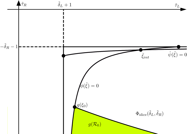
Figure 8: A sketch of $\phi(\tilde{\xi})=0$ and $\hat{\psi}(\tilde{\xi})=0$ where $\tilde{\xi}=g(\xi)$ with $0<\tilde{\delta}_{L}<1$ and $0<\tilde{\delta}_{R}<1$. The point $\tilde{\xi}_{\rm int}$ is the unique intersection of $\phi(\tilde{\xi})=0$ and $\hat{\psi}(\tilde{\xi})=0$. The point $\xi_{0}$ is as in Lemma 6.1.

6.2 Arguments leading to a proof of Theorem 2.14

Here we prove Theorem 2.14 after a sequence of lemmas.

Lemma 6.4.

Let $\xi\in\mathcal{R}_{n}$ for some $n\geq 1$. Then $g^{i}(\xi)\in\mathcal{R}_{n-i}$ for all $i=1,2,\ldots,n$.

Proof.

We have $\zeta_{n}(\xi)>0$ and $\zeta_{n+1}(\xi)\leq 0$ by (2.13). Thus $\zeta_{n-i}\mathopen{}\mathclose{{}\left(g^{i}(\xi)}\right)>0$ and $\zeta_{n-i+1}\mathopen{}\mathclose{{}\left(g^{i}(\xi)}\right)\leq 0$ by (2.12). Also $g^{i}(\xi)\in\Phi$ by Proposition 6.1. Thus $g^{i}(\xi)\in\mathcal{R}_{n-i}$ by (2.13). ∎

Lemma 6.5.

Let $\xi\in\Phi$ with $g(\xi)\in\mathcal{R}_{n-1}$ for some $n\geq 1$. Then $\xi\in\mathcal{R}_{n}$.

Proof.

We have $\zeta_{n-1}(g(\xi))>0$ and $\zeta_{n}(g(\xi))\leq 0$ by (2.13). Thus $\zeta_{n}(\xi)>0$ and $\zeta_{n+1}(\xi)\leq 0$ by (2.12). So $\xi\in\mathcal{R}_{n}$ because also $\xi\in\Phi$. ∎

Lemma 6.6.

Let $\xi\in\mathcal{R}_{n}$ for some $n\geq 1$. Then $\zeta_{0}(g(\xi))>0$.

Proof.

We have $\zeta_{n}(\xi)>0$ by (2.13), thus $\zeta_{1}\mathopen{}\mathclose{{}\left(g^{n-1}(\xi)}\right)>0$ by (2.12). Thus $\zeta_{1}(\xi)>0$ by Proposition 6.3 (recall the sign of $\zeta_{1}$ is the same as that of $\hat{\psi}$). That is, $\zeta_{0}(g(\xi))>0$. ∎

Lemma 6.7.

Let $\xi\in\Phi$ and write $g^{i}(\xi)=\mathopen{}\mathclose{{}\left(\tau_{L,i},\delta_{L,i},\tau_{R,i},\delta_{R,i}}\right)$ for each $i$. Then $\tau_{L,2}>\tau_{L}^{2}\tau_{R}^{2}$ and $\tau_{R,2}<\tau_{L}\tau_{R}$.

Proof.

By (2.10),

$$\tau_{L,2}=\tau_{R,1}^{2}-2\delta_{R,1}=\mathopen{}\mathclose{{}\left(\tau_{L}\tau_{R}-\delta_{L}-\delta_{R}}\right)^{2}-2\delta_{L}\delta_{R}\,,$$

which can be rearranged as

$$\tau_{L,2}=\mathopen{}\mathclose{{}\left(\tau_{L}\tau_{R}-\delta_{L}}\right)^{2}+\mathopen{}\mathclose{{}\left(\tau_{L}\tau_{R}-\delta_{R}}\right)^{2}-\tau_{L}^{2}\tau_{R}^{2}\,.$$

Then from the bounds in (2.2) we obtain $\tau_{L,2}>\tau_{L}^{2}\tau_{R}^{2}$. Also

$$\tau_{R,2}=\tau_{L,1}\tau_{R,1}-\delta_{L,1}-\delta_{R,1}<\tau_{L,1}\tau_{R,1}\,.$$

By substituting $\tau_{L,1}>1$ and $\tau_{R,1}>\tau_{L}\tau_{R}$ we obtain $\tau_{R,2}<\tau_{L}\tau_{R}$. ∎

Proof of Theorem 2.14.

Suppose for a contradiction that the $\mathcal{R}_{n}$ are not mutually disjoint. So there exists $\xi\in\mathcal{R}_{m}\cap\mathcal{R}_{n}$ for some $0\leq m<n$. This implies $g^{n-1}(\xi)\in\mathcal{R}_{1}$ by Lemma 6.4, and so $\hat{\psi}(g^{n-1}(\xi))>0$ (the sign of $\zeta_{1}$ is the same as that of $\hat{\psi}$). Also $g^{m}(\xi)\in\mathcal{R}_{0}$, so $\hat{\psi}(g^{m}(\xi))\leq 0$. By Proposition 6.3, $\hat{\psi}(g^{m+i}(\xi))\leq 0$ for all $i\geq 0$. In particular $\hat{\psi}(g^{n-1}(\xi))\leq 0$, and this is a contradiction. Therefore the $\mathcal{R}_{n}$ are mutually disjoint.

Now choose any $\xi\in\Phi_{\rm BYG}$. To verify (2.14) we show there exists $n\geq 0$ such that $\xi\in\mathcal{R}_{n}$. Certainly this is true if $\hat{\psi}(\xi)\leq 0$, because in this case $\xi\in\mathcal{R}_{0}$, so let us assume $\hat{\psi}(\xi)>0$. In view of Lemma 6.7, we consider the map $\tilde{g}:\mathbb{R}^{2}\to\mathbb{R}^{2}$ defined by

$$\tilde{g}(\tau_{L},\tau_{R})=\mathopen{}\mathclose{{}\left(\mathopen{}\mathclose{{}\left(\tau_{L}\tau_{R}}\right)^{2},\tau_{L}\tau_{R}}\right).$$

For any $j\geq 1$ the $j^{\rm th}$-iterate of $\tilde{g}$ is given explicitly by

$$\tilde{g}^{j}(\tau_{L},\tau_{R})=\mathopen{}\mathclose{{}\left(\mathopen{}\mathclose{{}\left(\tau_{L}\tau_{R}}\right)^{2k_{j}},\mathopen{}\mathclose{{}\left(\tau_{L}\tau_{R}}\right)^{k_{j}}}\right),$$

where $k_{j}=3^{j-1}$. Then Lemma 6.7 implies $\tau_{R,2j}<\mathopen{}\mathclose{{}\left(\tau_{L}\tau_{R}}\right)^{k_{j}}$ (using the notation of Lemma 6.7) and so $\tau_{R,2j}\to-\infty$ as $j\to\infty$. Thus there exists $m\geq 0$ such that $\tau_{R,m}\leq-2$. Then $\hat{\psi}(g^{m}(\xi))<0$ by Lemma 5.5. Now let $n\in\{1,2,\ldots,m\}$ be the smallest integer for which $\hat{\psi}(g^{n}(\xi))\leq 0$. Then $\hat{\psi}(g^{n-1}(\xi))>0$, so $\phi(g^{n}(\xi))>0$. That is, $g^{n}(\xi)\in\mathcal{R}_{0}$. Hence $\xi\in\mathcal{R}_{n}$, by $n$ applications of Lemma 6.5. This completes our verification of (2.14).

To show that $\mathcal{R}_{j}$ is non-empty for all $j\geq 0$, first observe $\hat{\psi}(\xi^{*})>0$. Also $\mathcal{R}_{0}$ is certainly non-empty. So for any $j\geq 1$ we can choose $\xi\in\Phi_{\rm BYG}$ sufficiently close to $\xi^{*}$ that $\hat{\psi}(g^{i}(\xi))>0$ for all $i=0,1,\ldots,j-1$. Again let $n\geq 1$ be the smallest integer for which $\hat{\psi}(g^{n}(\xi))\leq 0$. Then $n\geq j$ and $g^{n}(\xi)\in\mathcal{R}_{0}$. Thus $g^{n-j}(\xi)\in\mathcal{R}_{j}$ (by again using Lemma 6.5), i.e. $\mathcal{R}_{j}$ is non-empty.

Finally, choose any $\varepsilon>0$ and let $B_{\varepsilon}(\xi^{*})$ be the open ball in $\mathbb{R}^{4}$ centred at $\xi^{*}$ and with radius $\varepsilon$ using the Euclidean norm. We now show there exists $m\geq 1$ such that $\mathcal{R}_{n}\subset B_{\varepsilon}(\xi^{*})$ for all $n>m$. This will prove that $\mathcal{R}_{n}\to\{\xi^{*}\}$ as $n\to\infty$. Choose any $\xi\in\Phi$ with $\xi\notin B_{\varepsilon}(\xi^{*})$. It is simple exercise to show that $|\tau_{L}\tau_{R}|\geq 1+\frac{\varepsilon}{\sqrt{2}}$. Thus, as above, there exists $m\geq 0$ such that $\tau_{R,m}\leq-2$ and $\xi\in\mathcal{R}_{n}$ for some $n\leq m$. Hence for any $n>m$ the region $\mathcal{R}_{n}$ contains no points outside of $B_{\varepsilon}(\xi^{*})$. That is $\mathcal{R}_{n}\subset B_{\varepsilon}(\xi^{*})$ for all $n>m$ and therefore $\mathcal{R}_{n}\to\{\xi^{*}\}$ as $n\to\infty$. ∎

7 Positive Lyapunov exponents

For smooth maps Lyapunov exponents are usually defined in terms of the derivative of the map. The border-collision normal form $f_{\xi}$ is not differentiable on $x=0$, so instead we work with one-sided directional derivatives, §7.1. We then define Lyapunov exponents in terms of these derivatives, §7.2. This definition coincides with the familiar interpretation of Lyapunov exponents as the asymptotic rate of separation of nearby forward orbits [26]. Then in §7.3 we prove Theorem 2.2.

7.1 One-sided directional derivatives

Definition 7.1.

The one-sided directional derivative of a function $F:\mathbb{R}^{2}\to\mathbb{R}^{2}$ at $z\in\mathbb{R}^{2}$ in a direction $v\in\mathbb{R}^{2}$ is

$${\rm D}_{v}^{+}F(z)=\lim_{\delta\to 0^{+}}\frac{F(z+\delta v)-F(z)}{\delta},$$ (7.1)

if this limit exists.

The following result tells us that one-sided directional derivatives of the $n^{\rm th}$ iterate of (1.1) exist everywhere and for all $n\geq 1$. This follows from the piecewise-linearity and continuity of (1.1). For a proof see [26].

Lemma 7.1.

For any $\xi\in\mathbb{R}^{4}$, $z\in\mathbb{R}^{2}$, $v\in\mathbb{R}^{2}$, and $n\geq 1$, ${\rm D}_{v}^{+}f_{\xi}^{n}(z)$ exists.

7.2 Lyapunov exponents

In view of Lemma 7.1 we can use the following definition.

Definition 7.2.

The Lyapunov exponent of $f_{\xi}$ at $z\in\mathbb{R}^{2}$ in a direction $v\in\mathbb{R}^{2}$ is

$$\lambda(z,v)=\limsup_{n\to\infty}\frac{1}{n}\ln\mathopen{}\mathclose{{}\left(\mathopen{}\mathclose{{}\left\|{\rm D}_{v}^{+}f_{\xi}^{n}(z)}\right\|}\right).$$ (7.2)

If the forward orbit of $z$ does not intersect $x=0$, then ${\rm D}f_{\xi}^{n}(z)$ (the Jacobian matrix of $f_{\xi}^{n}$ at $z$) is well-defined for all $n\geq 1$. Moreover, ${\rm D}_{v}^{+}f_{\xi}^{n}(z)={\rm D}f_{\xi}^{n}(z)v$, so in this case (7.2) reduces to the usual expression given for smooth maps.

The following result is Theorem 2.1 of [8], except in [8] only forward orbits that do not intersect $x=0$ were considered. The generalisation to one-sided directional derivatives is elementary so we do not provide a proof. The proof in [8] is achieved by constructing an invariant expanding cone for multiplying vectors $v$ under the matrices $A_{L}$ and $A_{R}$. The derivative in (7.2) can be written as $v$ left-multiplied by $n$ matrices each of which is either $A_{L}$ or $A_{R}$. The cone implies the vector increases in norm each time it is multiplied by $A_{L}$ or $A_{R}$, so certainly the norm increases on average, i.e. $\lambda(z,v)>0$.

Proposition 7.2.

For any $\xi\in\Phi_{\rm BYG}$, $z\in\mathbb{R}^{2}$, and $v=(1,0)$,

$$\liminf_{n\to\infty}\frac{1}{n}\ln\mathopen{}\mathclose{{}\left(\mathopen{}\mathclose{{}\left\|{\rm D}_{v}^{+}f_{\xi}^{n}(z)}\right\|}\right)>0.$$ (7.3)

7.3 Arguments leading to a proof of Theorem 2.2

We are now ready to prove Theorem 2.2. Once we have constructed the set $\Delta$, the equality (2.16) follows from the arguments given in the proof of Lemma 6.2 of [8]. We reproduce these arguments here for convenience.

Proof of Theorem 2.2.

The set $\Lambda(\xi)$ is bounded because $X\in\Omega$ and $\Omega$ is bounded and forward invariant (Proposition 3.1). Also $\Lambda(\xi)$ is connected and invariant by the definition of an unstable manifold. With $v=(1,0)$ and any $z\in\Lambda(\xi)$, the Lyapunov exponent $\lambda(z,v)$ is well-defined by Lemma 7.1. Moreover $\lambda(z,v)>0$ by Proposition 7.3 and because the supremum limit is greater than or equal to the infimum limit.

It remains for us to prove part (iii). Here we assume $\delta_{R}<1$; also $\delta_{L}<1$ by Lemma 5.1. Since $\xi\in\mathcal{R}_{0}$ we have $\zeta_{1}(\xi)\leq 0$ and so $\psi(\xi)\geq 0$ by (4.4). Thus $f_{\xi}^{2}(T)$ lies on or to the left of $E^{s}(X)$ by Proposition 3.3. Let $Z$ denote the intersection of $E^{s}(X)$ with $\mathchoice{\overline{\displaystyle Tf_{\xi}^{2}(T)}}{\overline{\textstyle Tf_{\xi}^{2}(T)}}{\overline{\scriptstyle Tf_{\xi}^{2}(T)}}{\overline{\scriptscriptstyle Tf_{\xi}^{2}(T)}}$ (the line segment connecting $T$ and $f_{\xi}^{2}(T)$). Notice $\mathchoice{\overline{\displaystyle XT}}{\overline{\textstyle XT}}{\overline{\scriptstyle XT}}{\overline{\scriptscriptstyle XT}}$ and $\mathchoice{\overline{\displaystyle TZ}}{\overline{\textstyle TZ}}{\overline{\scriptstyle TZ}}{\overline{\scriptscriptstyle TZ}}$ are subsets of $W^{u}(X)$ while $\mathchoice{\overline{\displaystyle ZX}}{\overline{\textstyle ZX}}{\overline{\scriptstyle ZX}}{\overline{\scriptscriptstyle ZX}}$ is a subset of $W^{s}(X)$.

Let $\Delta_{0}$ be the filled triangle with vertices $X$, $T$, and $Z$, see Fig. 6-a. Also let $\Delta=\bigcup_{n=0}^{\infty}f_{\xi}^{n}(\Delta_{0})$. The set $\Delta$ is forward invariant, by definition, and has non-empty interior because it contains $\Delta_{0}$. As in [8], let $\tilde{\Delta}=\bigcap_{n=0}^{\infty}f_{\xi}^{n}(\Delta)$.

We now show $\Lambda(\xi)\subset\tilde{\Delta}$. Choose any $z\in\Lambda(\xi)$. Let $\{z_{k}\}$ be a sequence of points in $W^{u}(X)$ with $z_{k}\to z$ as $k\to\infty$. For each $k$, $f_{\xi}^{-n}(z_{k})\to X$ as $n\to\infty$, thus there exists $n_{k}\geq 1$ such that $f_{\xi}^{-{n_{k}}}(z_{k})\in\mathchoice{\overline{\displaystyle XT}}{\overline{\textstyle XT}}{\overline{\scriptstyle XT}}{\overline{\scriptscriptstyle XT}}$. Thus $f_{\xi}^{-{n_{k}}}(z_{k})\in\Delta_{0}$, so $z_{k}\in\Delta$. This is true for all $k$, thus $z\in\Delta$. But $z\in\Lambda(\xi)$ is arbitrary, thus $\Lambda(\xi)\subset\Delta$. Also $\Lambda(\xi)$ is forward invariant, thus $\Lambda(\xi)\subset\tilde{\Delta}$.

Finally we show $\tilde{\Delta}\subset\Lambda(\xi)$. The determinants $\delta_{L}$ and $\delta_{R}$ of the pieces of $f_{\xi}$ are both less than $1$, thus the area (Lebesgue measure) of $f_{\xi}^{n}(\Delta)$ converges to $0$ as $n\to\infty$. Now choose any $z\in\tilde{\Delta}$. Then $z\in f_{\xi}^{n}(\Delta)$ for all $n\geq 0$ and so the distance of $z$ to the boundary of $f_{\xi}^{n}(\Delta)$ converges to $0$ as $n\to\infty$. The boundary of $\Delta_{0}$ consists of $\mathchoice{\overline{\displaystyle XZ}}{\overline{\textstyle XZ}}{\overline{\scriptstyle XZ}}{\overline{\scriptscriptstyle XZ}}$, which lies in the part of $W^{s}(X)$ that converges linearly to $X$, and two line segments in $W^{u}(X)$. Consequently the boundary of $f_{\xi}^{n}(\Delta_{0})$ is contained in $\mathchoice{\overline{\displaystyle Xf_{\xi}^{n}(Z)}}{\overline{\textstyle Xf_{\xi}^{n}(Z)}}{\overline{\scriptstyle Xf_{\xi}^{n}(Z)}}{\overline{\scriptscriptstyle Xf_{\xi}^{n}(Z)}}\cup W^{u}(X)$ for all $n\geq 0$. Thus the boundary of $\Delta$ is contained in $\mathchoice{\overline{\displaystyle Zf_{\xi}(Z)}}{\overline{\textstyle Zf_{\xi}(Z)}}{\overline{\scriptstyle Zf_{\xi}(Z)}}{\overline{\scriptscriptstyle Zf_{\xi}(Z)}}\cup W^{u}(X)$, so the boundary of $f_{\xi}^{n}(\Delta)$ is contained in $\mathchoice{\overline{\displaystyle f_{\xi}^{n}(Z)f_{\xi}^{n+1}(Z)}}{\overline{\textstyle f_{\xi}^{n}(Z)f_{\xi}^{n+1}(Z)}}{\overline{\scriptstyle f_{\xi}^{n}(Z)f_{\xi}^{n+1}(Z)}}{\overline{\scriptscriptstyle f_{\xi}^{n}(Z)f_{\xi}^{n+1}(Z)}}\cup W^{u}(X)$ for all $n\geq 0$. But $\mathchoice{\overline{\displaystyle f_{\xi}^{n}(Z)f_{\xi}^{n+1}(Z)}}{\overline{\textstyle f_{\xi}^{n}(Z)f_{\xi}^{n+1}(Z)}}{\overline{\scriptstyle f_{\xi}^{n}(Z)f_{\xi}^{n+1}(Z)}}{\overline{\scriptscriptstyle f_{\xi}^{n}(Z)f_{\xi}^{n+1}(Z)}}$ converges to $X$, hence the distance of $z$ to $W^{u}(X)$ must be $0$. Thus $z\in\Lambda(\xi)$. But $z\in\tilde{\Delta}$ is arbitrary, thus $\tilde{\Delta}\subset\Lambda(\xi)$. This completes our demonstration of (2.16). ∎

8 Implementing the renormalisation recursively

In this section we work towards a proof of Theorem 2.3. First in §8.1 we use the unstable manifold of $X$ to construct a triangle $\Omega^{\prime}(\xi)$ that maps to $\Omega(g(\xi))$ under the affine transformation $h_{\xi}$ for converting $f_{\xi}^{2}$ to $f_{g(\xi)}$. In particular we show that $\Omega^{\prime}(\xi)$ is a subset of both $\Omega(\xi)$ and $\Pi_{\xi}$ and this allows us to implement the renormalisation recursively in §8.2.

8.1 Properties of the set mapping to $\Omega(g(\xi))$

Suppose $\xi\in\Phi$ with $\zeta_{1}(\xi)>0$ (equivalently $\psi(\xi)<0$). Then $f_{\xi}^{2}(T)$ lies to the right of $E^{s}(X)$ by Proposition 3.3. Thus $f_{\xi}^{3}(T)$ lies to the left of $E^{s}(X)$ (because $\lambda_{R}^{u}<0$). Now let $Q$ denote the intersection of $E^{u}(X)$ with the line through $f_{\xi}^{3}(T)$ and parallel to $E^{s}(X)$, see Fig. 6-b. Then let $\Omega^{\prime}(\xi)$ be the filled triangle with vertices $f_{\xi}(T)$, $f_{\xi}^{3}(T)$, and $Q$.

Lemma 8.1.

Let $\xi\in\Phi$ with $\zeta_{1}(\xi)>0$. Then

1. $\Omega^{\prime}(\xi)\subset\Pi_{\xi}$,

2. $\Omega^{\prime}(\xi)\cap f_{\xi}\mathopen{}\mathclose{{}\left(\Omega^{\prime}(\xi)}\right)=\varnothing$,

3. $f_{\xi}\mathopen{}\mathclose{{}\left(\Omega^{\prime}(\xi)}\right)\subset\mathopen{}\mathclose{{}\left\{(x,y)\in\mathbb{R}^{2}\,\big{|}\,x>0}\right\}$,

4. $h_{\xi}\mathopen{}\mathclose{{}\left(\Omega^{\prime}(\xi)}\right)=\Omega(g(\xi))$,

5. and if $\zeta_{0}(\xi)>0$ then $\Omega^{\prime}(\xi)\subset\Omega(\xi)$.

Proof.

Let $\Xi_{R}=\mathopen{}\mathclose{{}\left\{(x,y)\in\mathbb{R}^{2}\,\big{|}\,x>0}\right\}$ denote the open right half-plane and let $\Psi$ be the triangle with vertices $X$, $f_{\xi}(T)$, and $V$. We now prove parts (i)–(v) in order.

1. Observe $f_{\xi}(X)=X\in\Xi_{R}$, thus $X\in\Pi_{\xi}$ by (2.8). Similarly $f_{\xi}(V)\in\Xi_{R}$, thus $V\in\Pi_{\xi}$. Also $f_{\xi}^{2}(T)\in\Xi_{R}$, thus $f_{\xi}(T)\in\Pi_{\xi}$. That is, all vertices of $\Psi$ belong to $\Pi_{\xi}$, thus $\Psi\subset\Pi_{\xi}$ because these sets are convex.

   From (3.5) and (5.17) we find that the slope of the line through $T$ and $f_{\xi}^{2}(T)$ is $\frac{-\delta_{L}}{\tau_{L}-\lambda_{R}^{s}}$, which is negative, thus $f_{\xi}^{2}(T)$ lies to the left of $T$. Consequently $f_{\xi}^{3}(T)$ lies above $f_{\xi}(T)$. Also $f_{\xi}(T)$ lies above $V$ because

   $$f_{\xi}(T)_{2}-V_{2}=\frac{1-\delta_{R}}{\mathopen{}\mathclose{{}\left(1-\lambda_{R}^{s}}\right)\mathopen{}\mathclose{{}\left(1-\frac{1}{\lambda_{R}^{u}}}\right)}>0.$$

   Therefore $f_{\xi}^{3}(T)\in\Psi$. Thus $\Omega^{\prime}(\xi)\subset\Psi\subset\Pi_{\xi}$.

2. Observe $f_{\xi}(\Psi)$ is the quadrilateral with vertices $X$, $f_{\xi}(V)$, $f_{\xi}^{2}(T)$, and $T$. Thus $\Psi$ and $f_{\xi}(\Psi)$ intersect only at $X$. But $\Omega^{\prime}(\xi)\subset\Psi$ does not contain $X$, thus $\Omega^{\prime}(\xi)\cap f_{\xi}\mathopen{}\mathclose{{}\left(\Omega^{\prime}(\xi)}\right)=\varnothing$.

3. The left-most point of $f_{\xi}(\Psi)$ is $X\in\Xi_{R}$, thus $f_{\xi}\mathopen{}\mathclose{{}\left(\Omega^{\prime}(\xi)}\right)\subset f_{\xi}(\Psi)\subset\Xi_{R}$.

4. For the map $f_{\xi}^{2}$, the fixed point $X$ is a saddle with positive eigenvalues. Thus its unstable manifold has two dynamically independent branches. The branch that emanates to the left has its first and second kinks at $f_{\xi}(T)$ and $f_{\xi}^{3}(T)$. Let $\mathcal{B}$ denote this branch up to the second kink, that is $\mathcal{B}$ is the union of the line segments $\mathchoice{\overline{\displaystyle Xf_{\xi}(T)}}{\overline{\textstyle Xf_{\xi}(T)}}{\overline{\scriptstyle Xf_{\xi}(T)}}{\overline{\scriptscriptstyle Xf_{\xi}(T)}}$ and $\mathchoice{\overline{\displaystyle f_{\xi}(T)f_{\xi}^{3}(T)}}{\overline{\textstyle f_{\xi}(T)f_{\xi}^{3}(T)}}{\overline{\scriptstyle f_{\xi}(T)f_{\xi}^{3}(T)}}{\overline{\scriptscriptstyle f_{\xi}(T)f_{\xi}^{3}(T)}}$.

   By the conjugacy relation (4.2), $h_{\xi}(\mathcal{B})$ is part of one branch of the unstable manifold of the analogous fixed point of $f_{g(\xi)}$. Since $h_{\xi}$ flips points across the switching line (4.3), $h_{\xi}(\mathcal{B})$ is part of the unstable manifold of $Y$ (for the map $f_{g(\xi)}$). This branch has its first and second kinks at $D$ and $f_{g(\xi)}(D)$, thus $h_{\xi}(\mathcal{B})$ is the union of the line segments $\mathchoice{\overline{\displaystyle YD}}{\overline{\textstyle YD}}{\overline{\scriptstyle YD}}{\overline{\scriptscriptstyle YD}}$ and $\mathchoice{\overline{\displaystyle Df_{g(\xi)}(D)}}{\overline{\textstyle Df_{g(\xi)}(D)}}{\overline{\scriptstyle Df_{g(\xi)}(D)}}{\overline{\scriptscriptstyle Df_{g(\xi)}(D)}}$. By similar reasoning $Q$ maps under $h_{\xi}$ to the point $B$ of $f_{g(\xi)}$. This verifies part (iv).

5. The first components of $T$ and $D$ are $T_{1}=\frac{1}{1-\lambda_{R}^{s}}$ and $D_{1}=\frac{1}{1-\lambda_{L}^{s}}$. Observe $0<T_{1}<D_{1}$, thus $T$ lies between $(0,0)$ and $D$. By iterating these under $f_{R,\xi}$ we have that $f_{\xi}(T)$ lies on the line segment connecting $(1,0)$ and $f_{\xi}(D)$.

   Now suppose $\zeta_{0}(\xi)>0$. Then $f_{\xi}(T)\in\Omega(\xi)$ because $(1,0)\in\Omega(\xi)$, $f_{\xi}(D)\in\Omega(\xi)$, and $\Omega(\xi)$ is convex. Moreover, $f_{\xi}^{3}(T)\in\Omega(\xi)$ because $\Omega(\xi)$ is forward invariant (Proposition 3.1). Also $X\in\Omega(\xi)$ by Lemma 3.2. Thus the triangle with vertices $f_{\xi}(T)$, $f_{\xi}^{3}(T)$, and $X$ is contained in $\Omega(\xi)$ (again by the convexity of $\Omega(\xi)$). This triangle contains $\Omega^{\prime}(\xi)$, thus $\Omega^{\prime}(\xi)\subset\Omega(\xi)$ as required.

∎

8.2 Arguments leading to a proof of Theorem 2.3

Proof of Theorem 2.3.

Let $I_{n}=\{0,1,\ldots,2^{n}-1\}$. We use induction on $n$ to prove Theorem 2.3 and show that

$$\text{if $\zeta_{0}(\xi)>0$ then $S_{i}\subset\Omega(\xi)$ for all $i\in I_{n}$}.$$ (8.1)

With $n=0$ the statements in Theorem 2.3 are true trivially with $S_{0}=\Lambda(\xi)$. Also (8.1) is true because $\zeta_{0}(\xi)>0$ (since $\xi\in\mathcal{R}_{0}$) and $S_{0}\subset\Omega(\xi)$ by Lemma 3.2.

Now suppose the result is true for some $n\geq 0$; it remains for us to verify the result for $n+1$. Choose any $\xi\in\mathcal{R}_{n+1}$. Then $g(\xi)\in\mathcal{R}_{n}$ by Lemma 6.4. By the induction hypothesis applied to the point $g(\xi)$, we have $g^{n+1}(\xi)\in\mathcal{R}_{0}$ and there exist mutually disjoint sets $\tilde{S}_{0},\tilde{S}_{1},\ldots,\tilde{S}_{2^{n}-1}\subset\mathbb{R}^{2}$ with $f_{g(\xi)}\mathopen{}\mathclose{{}\left(\tilde{S}_{i}}\right)=\tilde{S}_{(i+1)\,{\rm mod}\,2^{n}}$ and

$$f_{g(\xi)}^{2^{n}}\big{|}_{\tilde{S}_{i}}~{}\text{is affinely conjugate to}~{}f_{g^{n+1}(\xi)}\big{|}_{\Lambda(g^{n+1}(\xi))}$$ (8.2)

for all $i\in I_{n}$. Also $\zeta_{0}(g(\xi))>0$ by Lemma 6.6, thus by (8.1) the induction hypothesis also gives $\tilde{S}_{i}\subset\Omega(g(\xi))$ for all $i\in I_{n}$.

Let $S_{2i}=h_{\xi}^{-1}\mathopen{}\mathclose{{}\left(\tilde{S}_{i}}\right)$ for each $i\in I_{n}$ (these sets are mutually disjoint because $h_{\xi}$ is a homeomorphism). Let $S_{2i+1}=f_{\xi}(S_{2i})$ for each $i\in I_{n}$ (these sets are mutually disjoint because $f_{\xi}$ is a homeomorphism). For any $i,j\in I_{n}$ we have $S_{2i}\subset\Omega^{\prime}(\xi)$ by Lemma 8.1(iv) and $S_{2j+1}\cap\Omega^{\prime}(\xi)=\varnothing$ by Lemma 8.1(ii), so $S_{2i}\cap S_{2j+1}=\varnothing$. Therefore the sets $S_{0},S_{1},\ldots,S_{2^{n+1}-1}$ are mutually disjoint.

For each $i\in I_{n}$, $S_{2i}\subset\Pi_{\xi}$ by Lemma 8.1(i), so

$$f_{\xi}^{2}\big{|}_{S_{2i}}~{}\text{is affinely conjugate to}~{}f_{g(\xi)}\big{|}_{\tilde{S}_{i}}$$ (8.3)

by Proposition 4.1. Also $f_{\xi}^{2}(S_{2i})=S_{2i+2\,{\rm mod}\,2^{n+1}}$, so $f_{\xi}(S_{2i+1})=f_{R,\xi}(S_{2i+1})=S_{2i+2\,{\rm mod}\,2^{n+1}}$ using also Lemma 8.1(iii). Thus

$$f_{\xi}^{2}\big{|}_{S_{2i+1}}~{}\text{is affinely conjugate to}~{}f_{\xi}^{2}\big{|}_{S_{2i}}$$

using $f_{R,\xi}$ as the affine transformation. By further use of (4.2) we have that $f_{\xi}^{2^{n+1}}\big{|}_{S_{2i}}$ and $f_{\xi}^{2^{n+1}}\big{|}_{S_{2i+1}}$ are affinely conjugate to $f_{g(\xi)}^{2^{n}}\big{|}_{\tilde{S}_{i}}$, thus also to $f_{g^{n+1}(\xi)}\big{|}_{\Lambda(g^{n+1}(\xi))}$ by (8.2) (this verifies (2.18) for $n+1$).

The induction hypothesis also implies

$$\bigcup_{i=0}^{2^{n}-1}\tilde{S}_{i}={\rm cl}\mathopen{}\mathclose{{}\left(W^{u}(\gamma_{n})}\right),$$ (8.4)

where $\gamma_{n}$ is a periodic solution of $f_{g(\xi)}$ with symbolic itinerary $\mathcal{F}^{n}(R)$. By (4.2), $h_{\xi}^{-1}(\gamma_{n})$ is a periodic solution of $f_{\xi}^{2}$. Since $h_{\xi}$ flips the left and right half-planes, see (4.3), the symbolic itinerary of $h_{\xi}^{-1}(\gamma_{n})$ is obtained by swapping $L$ and $R$’s in $\mathcal{F}^{n}(R)$. Then $\gamma_{n+1}=h_{\xi}^{-1}(\gamma_{n})\cup f_{\xi}\mathopen{}\mathclose{{}\left(h_{\xi}^{-1}(\gamma_{n})}\right)$ is a periodic solution of $f_{\xi}$ and since $f_{\xi}\mathopen{}\mathclose{{}\left(h_{\xi}^{-1}(\gamma_{n})}\right)$ is contained in the right half-plane (Lemma 8.1(iii)) its symbolic itinerary is obtained by further replacing each $L$ with $LR$ and each $R$ with $RR$, hence $\gamma_{n+1}$ has symbolic itinerary $\mathcal{F}^{n+1}(R)$. Also by (8.3) and (8.4),

$$\bigcup_{i=0}^{2^{n+1}-1}S_{i}={\rm cl}\mathopen{}\mathclose{{}\left(W^{u}(\gamma_{n+1})}\right),$$

which verifies (2.19) for $n+1$. Finally, if $\zeta_{0}(\xi)>0$ then for all $i\in I_{n}$ we have $S_{2i}\subset\Omega(\xi)$ by Lemma 8.1(v) and $S_{2i+1}\subset\Omega(\xi)$ because $\Omega(\xi)$ is forward invariant verifying (8.1) for $n+1$. ∎

9 Discussion

In this paper we have shown how part of the parameter space of (1.1) naturally divides into regions $\mathcal{R}_{0},\mathcal{R}_{1},\ldots$. As demonstrated by Theorem 2.3, renormalisation enables us to describe the dynamics in each $\mathcal{R}_{n}$ with $n\geq 1$ based on knowledge of the dynamics in $\mathcal{R}_{0}$. Theorem 2.2 describes the dynamics in $\mathcal{R}_{0}$, but is incomplete. It remains to show the attractor $\Lambda$ is unique and satisfies stronger notions of chaos throughout $\mathcal{R}_{0}$. Also we would like to extend the results to high-dimensional maps.

Finally we comment on the analogy of Feigenbaum’s constant for our renormalisation by looking at the rate at which the regions $\mathcal{R}_{n}$ converge to the fixed point $\xi^{*}$. The $4\times 4$ Jacobian matrix ${\rm D}g(\xi^{*})$ has exactly one unstable eigenvalue: $2$. It follows that the diameter of $\mathcal{R}_{n}$ divided by the diameter of $\mathcal{R}_{n+1}$ tends, as $n\to\infty$, to the constant $2$.

References

- [1] S. Banerjee and C. Grebogi. Border collision bifurcations in two-dimensional piecewise smooth maps. Phys. Rev. E, 59(4):4052–4061, 1999.
- [2] S. Banerjee, J.A. Yorke, and C. Grebogi. Robust chaos. Phys. Rev. Lett., 80(14):3049–3052, 1998.
- [3] P. Collet and J.-P. Eckmann. Iterated Maps of the Interval as Dynamical Systems. Birkhäuser, Boston, 1980.
- [4] W. de Melo and S. van Strien. One-Dimensional Dynamics. Springer-Verlag, New York, 1993.
- [5] M. di Bernardo, C.J. Budd, A.R. Champneys, and P. Kowalczyk. Piecewise-smooth Dynamical Systems. Theory and Applications. Springer-Verlag, New York, 2008.
- [6] P. Glendinning. Bifurcation from stable fixed point to 2D attractor in the border collision normal form. IMA J. Appl. Math., 81(4):699–710, 2016.
- [7] P. Glendinning. Robust chaos revisited. Eur. Phys. J. Special Topics, 226(9):1721–1738, 2017.
- [8] P.A. Glendinning and D.J.W. Simpson. A constructive approach to robust chaos using invariant manifolds and expanding cones. Discrete Contin. Dyn. Syst., 41(7):3367–3387, 2021.
- [9] J. Graczyk and G. Swiatek. Generic hyperbolicity in the logistic family. Ann. Math., 146(1):1–52, 1997.
- [10] C. Grebogi, E. Ott, and J.A. Yorke. Crises, sudden changes in chaotic attractors, and transient chaos. Phys. D, 7:181–200, 1983.
- [11] S. Ito, S. Tanaka, and H. Nakada. On unimodal linear transformations and chaos II. Tokyo J. Math., 2:241–259, 1979.
- [12] R. Lozi. Un attracteur étrange(?) du type attracteur de Hénon. J. Phys. (Paris), 39(C5):9–10, 1978. In French.
- [13] M. Lyubich. Dynamics of quadratic polynomials, I-II. Acta. Math., 178:185–297, 1997.
- [14] R.S. MacKay. Renormalisation in Area-preserving Maps. World Scientific, Singapore, 1993.
- [15] J. Milnor. On the concept of attractor. Commun. Math. Phys., 99:177–195, 1985.
- [16] M. Misiurewicz. Strange attractors for the Lozi mappings. In R.G. Helleman, editor, Nonlinear dynamics, Annals of the New York Academy of Sciences, pages 348–358, New York, 1980. Wiley.
- [17] H.E. Nusse and J.A. Yorke. Border-collision bifurcations including “period two to period three” for piecewise smooth systems. Phys. D, 57:39–57, 1992.
- [18] J. Palis and F. Takens. Hyperbolicity and sensitive chaotic dynamics at homoclinic bifurcations. Cambridge University Press, New York, 1993.
- [19] A. Pumariño, J.A. Rodríguez, and E. Vigil. Renormalization of two-dimensional piecewise linear maps: Abundance of 2-D strange attractors. Discrete Contin. Dyn. Syst., 38(2):941–966, 2018.
- [20] A. Pumariño, J.Á. Rodríguez, and E. Vigil. Persistent two-dimensional strange attractors for a two-parameter family of expanding baker maps. Discrete Contin. Dyn. Syst. Ser. B, 24(2):657–670, 2019.
- [21] T. Puu and I. Sushko, editors. Business Cycle Dynamics: Models and Tools. Springer-Verlag, New York, 2006.
- [22] R.C. Robinson. An Introduction to Dynamical Systems. Continuous and Discrete. Prentice Hall, Upper Saddle River, NJ, 2004.
- [23] D.J.W. Simpson. Sequences of periodic solutions and infinitely many coexisting attractors in the border-collision normal form. Int. J. Bifurcation Chaos, 24(6):1430018, 2014.
- [24] D.J.W. Simpson. Border-collision bifurcations in . SIAM Rev., 58(2):177–226, 2016.
- [25] D.J.W. Simpson. Unfolding homoclinic connections formed by corner intersections in piecewise-smooth maps. Chaos, 26:073105, 2016.
- [26] D.J.W. Simpson. Detecting invariant expanding cones for generating word sets to identify chaos in piecewise-linear maps. Submitted., 2020.
- [27] D.J.W. Simpson and J.D. Meiss. Neimark-Sacker bifurcations in planar, piecewise-smooth, continuous maps. SIAM J. Appl. Dyn. Sys., 7(3):795–824, 2008.
- [28] D. Veitch and P. Glendinning. Explicit renormalisation in piecewise linear bimodal maps. Phys. D, 44:149–167, 1990.
- [29] Z.T. Zhusubaliyev, E. Mosekilde, S. Maity, S. Mohanan, and S. Banerjee. Border collision route to quasiperiodicity: Numerical investigation and experimental confirmation. Chaos, 16(2):023122, 2006.