MirrorWiC: On Eliciting Word-in-Context Representations
from Pretrained Language Models

Abstract

Recent work indicated that pretrained language models (PLMs) such as BERT and RoBERTa can be transformed into effective sentence and word encoders even via simple self-supervised techniques. Inspired by this line of work, in this paper we propose a fully unsupervised approach to improving word-in-context (WiC) representations in PLMs, achieved via a simple and efficient WiC-targeted fine-tuning procedure: MirrorWiC. The proposed method leverages only raw texts sampled from Wikipedia, assuming no sense-annotated data, and learns context-aware word representations within a standard contrastive learning setup. We experiment with a series of standard and comprehensive WiC benchmarks across multiple languages. Our proposed fully unsupervised MirrorWiC models obtain substantial gains over off-the-shelf PLMs across all monolingual, multilingual and cross-lingual setups. Moreover, on some standard WiC benchmarks, MirrorWiC is even on-par with supervised models fine-tuned with in-task data and sense labels.

1 Introduction

Pretrained Language Models (PLMs) such as BERT Devlin et al. (2019) and RoBERTa Liu et al. (2019) provide dynamic contextual representations; they induce token-level lexical representations that capture the impact of the word’s context on its embedding. Recent studies have assessed the PLMs by probing into their off-the-shelf representation/feature space Garí Soler et al. (2019); Wiedemann et al. (2019); Reif et al. (2019); Garí Soler and Apidianaki (2021). While off-the-shelf PLMs already offer a useful contextualised lexical semantic space, their contextualised representation spaces suffer from instability and anisotropy Mickus et al. (2020); Pedinotti and Lenci (2020). As a consequence, they usually fall far behind the performance of the same PLM fine-tuned with (i) sense annotations Hadiwinoto et al. (2019); Blevins and Zettlemoyer (2020) or (ii) external (e.g., WordNet) knowledge Levine et al. (2020).

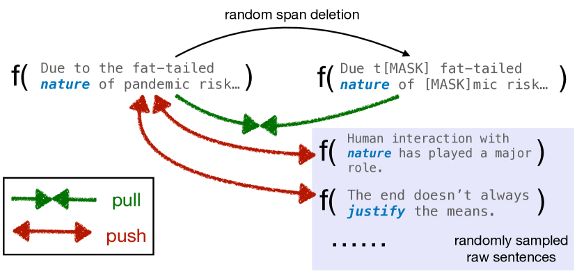
Figure 1: An illustrative overview of the MirrorWiC method, based on contrastive learning, for eliciting better word-in-context (WiC) representations from pretrained language models. We augment a randomly selected WiC instance with random span masking and apply dropout to the hidden states to create two slightly different representations of the base instance. These two representations form a positive pair for contrastive fine-tuning. During fine-tuning, we pull the representations of each positive pair closer together, while at the same time pushing away representations of other WiC instances, serving as negative examples.

However, PLMs have been shown to actually store more lexical and sentence-level information than what can be directly extracted from their off-the-shelf variants. In simple words, this knowledge must be ‘unlocked’ or exposed via additional adaptive fine-tuning Ruder (2021). For instance, while off-the-shelf PLMs are not directly effective as universal sentence encoders, it is possible to convert them into such encoders through supervised Reimers and Gurevych (2019a); Feng et al. (2020); Liu et al. (2021a) or self-supervised fine-tuning Carlsson et al. (2021); Liu et al. (2021b); Gao et al. (2021) based on the contrastive learning paradigm.

The fundamental limitation of extracting contextual features/representations directly from the layers of the off-the-shelf PLMs is the mismatch between their (pre)training objectives and the feature extraction method. In other words, the contextual representations, typically extracted as the averages over the top four layers of a base PLM Liu et al. (2020); Garí Soler and Apidianaki (2021), can be seen as a by-product of training a language model, and are not directly optimised for contextual sensitivity. Inspired by the previous work on adaptive fine-tuning for word and sentence representations Liu et al. (2021b), we propose a simple self-supervised technique termed MirrorWiC: it rewires input PLMs to provide improved word-in-context (WiC) representations.

Unlike prior work on fine-tuning towards improving WiC representations, our MirrorWiC procedure disposes of any sense labels, annotated task data, and any external knowledge, and elicits improved WiC representations from PLMs in a fully unsupervised way. We design a contrastive learning framework that directly optimises the contextual representations (i.e., the top four hidden layers of the input PLM) that are also the feature space at inference time; see Figure 1 and Table 1. MirrorWiC relies on the sets of positive and negative pairs, where the positive pairs are created by pairing an input sequence (which contains a target word) with its slightly altered variant. This altered sequence is obtained via random span masking and the resulting representations for this pair are further altered by dropout. The negative pairs are then simply the same or different word’s contextual representations in a different context; Figure 1. These pairs for fine-tuning are mined from raw Wikipedia sentences. To understand why MirrorWiC works so well, we provide ablation studies on the design choices (including dropout rate, random span masking, etc.) and layer-wise analyses and visualisation on MirrorWiC’s effects on embedding properties such as isotropy.

Contributions. 1) We present a simple yet extremely effective unsupervised MirrorWiC technique for eliciting contextual lexical knowledge. 2) Our experiments on a range of English, multilingual, and cross-lingual context-sensitive lexical benchmarks demonstrate that MirrorWiC achieves consistent and substantial improvements over different baseline PLMs, indicating its robustness and wide applicability. 3) We offer extensive analyses and additional insights into the inner workings of MirrorWiC, and its impact on the contextual representation space. We release our code at github.com/cambridgeltl/MirrorWiC.

2 Related Work and Background

Word-in-Context Representations. Modelling context influence on lexical meaning and creating context-aware word representations is a long-standing research goal in lexical semantics. One direction is to create discrete sense embeddings according to a fixed sense inventory such as WordNet. These embeddings can be created from the attributes in the sense inventory such as glosses Chen et al. (2014) or from the knowledge structure Camacho-Collados et al. (2016). We point to Camacho-Collados and Pilehvar (2018) for a thorough survey on sense embeddings. Such sense representations require a fixed and discrete sense inventory and might not be sensitive enough to the the dynamic and fluid nature of contextual changes.

More recently, PLMs provide dynamic and continuous contextual representations, not tied to predefined sense inventories, computed as a function of both the target word and its context. The use of PLMs has resulted in further progress on a range of context-aware evaluation benchmarks Pilehvar and Camacho-Collados (2019); Wang et al. (2019); Raganato et al. (2020). A body of work has aimed to enrich context-aware and sense information in the PLMs by injecting such knowledge (e.g., sense annotations from predefined sense inventories) at pretraining stage Levine et al. (2020) or during inference Loureiro and Jorge (2019). Other work has attempted at combining/ensembling multiple contextualised and static type-level embeddings to refine the contextualised representation space (Liu et al., 2020; Xu et al., 2020).

Inducing Text Representations from PLMs via Self-Supervision. Recently, there has been growing interest in learning completely unsupervised sentence representations from PLMs using contrastive learning techniques (Carlsson et al., 2021; Liu et al., 2021b; Gao et al., 2021; Yan et al., 2021; Kim et al., 2021; Zhang et al., 2021). Similar to the supervised approaches such as Sentence-BERT Reimers and Gurevych (2019b) or SapBERT Liu et al. (2021a), the idea is to transform an input PLM into an effective sentence encoder via additional fine-tuning. During self-supervised contrastive fine-tuning, the model learns from identical or automatically modified text sequences (treated as positive examples), and regards different sentences as negative pairs. MirrorBert (Liu et al., 2021b) is a general self-supervised contrastive fine-tuning framework that transforms off-the-shelf PLMs into effective word and sentence encoders. Our proposed MirrorWiC method can be seen as an extension of MirrorBert, now focused on eliciting improved word-in-context representations and context-sensitive lexical tasks.

model	representations fine-tuned	representations extracted
off-the-shelf PLMs	([CLS] +) language modelling head	word token average (top four layers)
MirrorBert	[CLS]/mean-pooling	[CLS]/mean-pooling
MirrorWiC	word token average (top four layers)	word token average (top four layers)

Table 1: MirrorWiC benefits from the consistency of representations at (i) fine-tuning and (ii) feature extraction and inference: both are focused on word-in-context (WiC) representations.

Step 1: Automatic dataset creation for WiC fine-tuning
$({\color[rgb]{0,0,0}x_{1}},{\color[rgb]{1,0,1}y_{1}})$	(Due to the fat-tailed nature of pandemic risk, …, $1$)
$({\color[rgb]{0,0,0}\overline{x}_{1}},{\color[rgb]{1,0,1}\overline{y}_{1})}$	(Due to the fat-tailed nature of pandemic risk, …, $1$)
…	…
$({\color[rgb]{0,0,0}x_{i}},{\color[rgb]{1,0,1}y_{i}})$	(Human interaction with nature has played a major role., $i$)
$({\color[rgb]{0,0,0}\overline{x}_{i}},{\color[rgb]{1,0,1}\overline{y}_{i}})$	(Human interaction with nature has played a major role., $i$)
…	…
$({\color[rgb]{0,0,0}x_{N}},{\color[rgb]{1,0,1}y_{N}})$	(The end doesn’t always justify the means., $N$)
$({\color[rgb]{0,0,0}\overline{x}_{N}},{\color[rgb]{1,0,1}\overline{y}_{N}})$	(The end doesn’t always justify the means., $N$)
Step 2: Random span masking
$({\color[rgb]{0,0,0}x_{1}},{\color[rgb]{1,0,1}y_{1}})$	(Due to the fat-tailed nature of pandemic risk, …, $1$)
$({\color[rgb]{0,0,0}\overline{x}_{1}},{\color[rgb]{1,0,1}\overline{y}_{1}})$	(Due _e fat-tailed nature of pandemic _ …, $1$)
…	…
$({\color[rgb]{0,0,0}x_{i}},{\color[rgb]{1,0,1}y_{i}})$	(Human interaction with nature has played a major role., $i$)
$({\color[rgb]{0,0,0}\overline{x}_{i}},{\color[rgb]{1,0,1}\overline{y}_{i})}$	(Human intera_ with nature has play_major role., $i$)
…	…
$({\color[rgb]{0,0,0}x_{N}},{\color[rgb]{1,0,1}y_{N}})$	(the end does not always justify The means.,$N$)
$({\color[rgb]{0,0,0}\overline{x}_{N}},{\color[rgb]{1,0,1}\overline{y}_{N})}$	(The end does_always justify _eans., $N$)

Table 2: Upper: the automatically generated labelled dataset for fine-tuning PLMs towards learning better word-in-context representations. Bold denotes the target word. Lower: data augmentation via random span masking. ‘_’ denotes the ‘[MASK]’ token.

3 MirrorWiC: Methodology

Baseline WiC Representations. Prior work directly extracts word-in-context representations from the parameters of the off-the-shelf PLMs. The most effective (empirically validated) strategy is 1) averaging the representations from the top four PLM’s layers, and 2) then taking either the first constituent subword from the PLM’s vocabulary to represent the target word, or further averaging the representations of the word’s constituent subwords (Liu et al., 2020; Garí Soler and Apidianaki, 2021).

3.1 Self-Supervised WiC Fine-Tuning

We hypothesise that it is possible to convert the input PLM into an improved WiC encoder through adaptive (self-supervised) fine-tuning. Given a set of raw sentences without labels, how do we tune the PLMs to further expose their word-in-context knowledge? Inspired by MirrorBert (Liu et al., 2021b), we apply a self-supervised contrastive learning scheme to elicit better word-in-context representations. We fine-tune the input PLM by contrasting the representations of different word-in-context pairs while pulling representations of a self-duplicated word-in-context pair closer in the representation space (see Figure 1).

Data Creation. Given a set of $N$ non-duplicated sentences, we randomly select a word in each sentence as the target word: i.e., the sentences become a set of ‘word-in-context instances’. We then follow MirrorBert and generate a labelled dataset by duplicating each instance in the set and assigning identical labels to identical instances and different labels to different word-in-contexts (Table 2, upper half): $\mathcal{D}=\{(x_{1},y_{1}),(\overline{x}_{1},\overline{y}_{1}),\ldots,(x_{N},y_{N}),(\overline{x}_{N},\overline{y}_{N})\}$, where $\forall i=1,\ldots N$, it holds $x_{i}=\overline{x}_{i},y_{i}=\overline{y}_{i}$.

Data Augmentation. We further follow MirrorBert to create a slightly altered (or augmented) ‘view’ of the same text sequence: we randomly replace a span of text with ‘[MASK]’ in all duplicated examples. There is a fundamental difference to MirrorBert where such ‘random span masking’ technique is applied on sentences; for word-in-context, we keep the target word intact (otherwise the semantics changes drastically) and randomly replace a span of length $K$ on both sides of the target word; see Table 2 (lower half). Besides random span masking, the dropout modules in the Transformer layers also slightly and randomly alter the representations of each word-in-context instance. They serve as another source of data augmentation to further perturb the word-in-context representations. After both input space augmentation (random span masking) and feature space augmentation (dropout layers embedded in the Transformer layers), the resulting embeddings of even a positive pair will be slightly different.

Contrastive Fine-Tuning. Following the feature extraction procedure from off-the-shelf PLMs, we compute the average of hidden states from the PLM’s top four layers, and then take the average of all token(s) that correspond to the target word, as the word-in-context representation. Let $f(\cdot)$ denote the encoder which outputs such WiC representation. We leverage InfoNCE (Oord et al., 2018) to cluster/attract the positive pairs together and push away the negative pairs in the embedding space:

$$\mathcal{L}=-\sum_{i=1}^{N}\log\frac{\exp(\cos(f(x_{i}),f(\overline{x}_{i}))/\tau)}{\displaystyle\sum_{x_{j}\in\mathcal{N}_{i}}\exp(\cos(f(x_{i}),f(x_{j}))/\tau)}.$$ (1)

where $\tau$ is a tunable temperature; $\mathcal{N}_{i}$ denotes all negatives of $x_{i}$, which includes all $x_{j},\overline{x}_{j}$ where $i\neq j$ in the current data batch (i.e., $|\mathcal{N}_{i}|=N-2$). Intuitively, the numerator is the similarity of the self-duplicated pair (a positive pair) and the denominator is the sum of the similarities between $x_{i}$ and all other strings besides $\overline{x}_{i}$ (negative pairs).

For positive pairs, though one sequence in the pair is slightly altered via random span masking and the representations go through dropout, the encoding function $f(\cdot)$ should learn an invariant mapping and reconstruct the correct semantics from the noise Liu et al. (2021b). Most negative examples contain different target words and different contexts (e.g., $x_{1}$ and $x_{N}$ in Table 2). Naturally, such pairs are of different meanings and the model should produce different representations.Note that it is possible to also have the same target word appearing in different contexts as a negative pair (e.g., $x_{1}$ and $x_{i}$ in Table 2). If the pair indeed has very different semantics (of a different sense), then pushing them apart is actually desirable. However, even if the items in the pair happen to have similar meanings, our learning objective still instructs the model to push them away from each other. Our rationale and decision here are based on the following: (1) Such false negative pairs can act as a regularisation; and (2) in essence, one could argue that all distinct word-in-context instances have slightly different meanings since sense is a continuous function of word and context.

4 Experimental Setup

WiC Evaluation. We evaluate MirrorWiC on a range of context-sensitive lexical semantic tasks in monolingual English settings, as well as in multilingual and cross-lingual settings.

For English, we evaluate on two similarity-based tasks: Usim and CoSimLex; two word-in-context classification tasks: WiC and WiC-TSV; and one-shot Word Sense Disambiguation (WSD). Usim (Erk et al., 2013) measures the similarity between two instances of the same word occurring in two different sentential contexts. CoSimLex Armendariz et al. (2020) measures the change in similarity between two different words appearing in two different contexts: paragraphs. We follow the standard evaluation protocol, computing the cosine similarity of the contextual word representations and comparing them against human-elicited scores via Spearman’s rank correlation ($\rho$).

The WiC classification task (Pilehvar and Camacho-Collados, 2019) challenges a model to make a binary decision on whether or not the same target word has the same meaning in two different contexts. The WiC-TSV (TSV) task (Breit et al., 2021) extends the original WiC to multiple domains with three different subtasks. In TSV-1, the task is to decide if the intended sense of the target word in the context matches the target sense described by the definition. In TSV-2, the model must identify if the intended sense (in the context) is the hyponym of the provided hypernyms. TSV-3 combines the previous two subtasks (see Breit et al. (2021) for further details).

The WSD task Navigli (2009); Raganato et al. (2017) requires a system to select the correct label for a given target word in context from a candidate set of all possible meanings for this target word. To evaluate the feature space of the models in WSD, we create a one-shot setting where we provide one context example per label and perform nearest neighbour search over contextual word representations from the candidate labels. We directly test the models on the concatenated ALL test set from Raganato et al. (2017) without access to training and development data.

We also perform multilingual and cross-lingual evaluation on XL-WiC (Raganato et al., 2020) and AM2iCo (Liu et al., 2021c). XL-WiC provides WiC-style evaluations in multiple languages. AM2iCo extends XL-WiC to lower-resource languages, adds more difficult adversarial examples, and enables cross-lingual evaluations. For brevity, we show results for four typologically diverse languages both from XL-WiC (zh, ko, hr, et); and four languages in AM2iCo (zh, ka, ja, ar).

For WiC, TSV, XL-WiC and AM2iCo, our main experiments follow the unsupervised method from Pilehvar and Camacho-Collados (2019): we compute cosine similarity between the contextual word representations in each pair, and search for a threshold to divide true (i.e., same meaning) and false instances on the development set in each task. We report accuracy scores in the main paper, while additional area-under-curve (AUC) scores are available in Section A.1.

Underlying PLMs. We experiment with several standard input PLMs for English, but we remind the reader that the MirrorWiC framework is applicable with a wide range of PLMs: 1) BERT Devlin et al. (2019) as a standard choice for WiC representation learning and evaluation Raganato et al. (2020); 2) RoBERTa Liu et al. (2019) as an optimised and improved PLM; and 3) DeBERTa He et al. (2020) as a more recent PLM that achieves state-of-the-art results in a range of natural language understanding tasks Wang et al. (2019). For all non-English experiments, unless noted otherwise, we rely on multilingual BERT (mBERT) as the underlying PLM (see Section A.2).

Fine-Tuning Details. We largely follow the MirrorBert fine-tuning setup Liu et al. (2021b), using 10k sentences randomly drawn from Wikipedia as the MirrorWiC fine-tuning corpus. For monolingual models, we sample 10k sentences from the corresponding Wikipedia of that language. For cross-lingual models, we sample 5k sentences from English Wikipedia and 5k from Wikipedia of each target language. We train all models with AdamW Loshchilov and Hutter (2019) with a learning rate of 2e-5 for 1 epoch. The $\tau$ in Equation 1 is set to $0.04$. We set $K$ (random span masking rate) to $10$, $0$ and $1$ for BERT, RoBERTa and DeBERTa respectively. The respective dropout rates are $0.4$, $0.3$ and $0.3$ for BERT, RoBERTa and DeBERTa. All hyper-parameters are tuned on the development set of WiC and kept unchanged for all other experiments. We refer the reader to the Appendix (Table 13) for a full listing of hyperparameters along with their search space.

5 Results and Discussion

model$\downarrow$, dataset$\rightarrow$	Usim ($\rho$)	WiC (acc)	TSV-1 (acc)	TSV-2 (acc)	TSV-3 (acc)	CoSimLex ($\rho$)	One-shot WSD (acc)
Sentence-BERT	23.57	61.91	62.46	59.64	62.72	-	42.63
MirrorBert	23.21	64.10	66.32	64.78	66.32	-	44.93
BERT	54.52	68.49	61.69	60.66	61.95	76.2	52.90
+ MirrorWiC	61.82	71.94	69.15	66.06	68.38	77.41	57.10
RoBERTa	50.25	66.77	55.52	56.55	57.58	75.64	51.38
+ MirrorWiC	57.95	71.15	69.92	67.60	71.70	77.27	56.51
DeBERTa	54.77	66.14	59.38	59.89	60.41	72.06	53.99
+ MirrorWiC	62.79	71.78	70.95	67.86	71.20	77.70	59.02

Table 3: Results across a collection of context-aware lexical semantic tasks in English.

5.1 Main Results: Evaluation on English

The main results are provided in Table 3 and Table 4. Most notably, we observe consistent and substantial gains over all unsupervised baselines, including the off-the-shelf PLMs without MirrorWiC fine-tuning. While the underlying PLMs, as suggested by prior work Garí Soler and Apidianaki (2021), do encode a wealth of sense-related knowledge, that knowledge can be further exposed via the proposed context-aware MirrorWiC fine-tuning procedure.

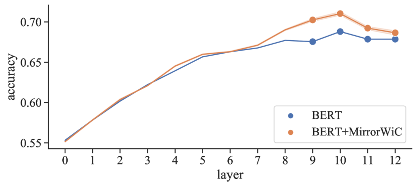
(a) BERT layer-wise accuracy; WiC dev

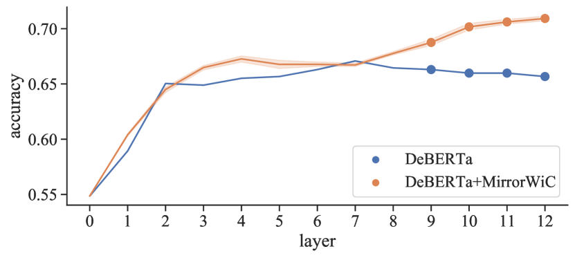
(b) DeBERTa layer-wise accuracy; WiC dev

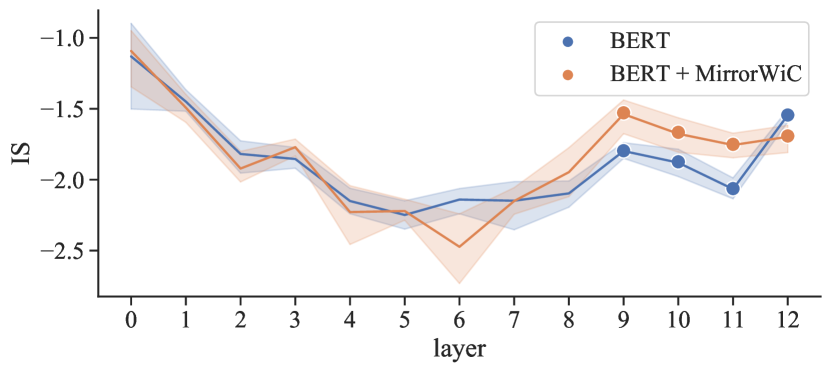
(c) BERT isotropy (higher is better)

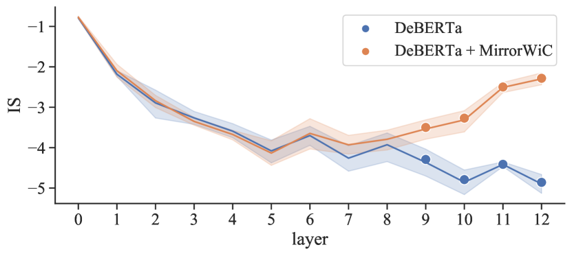
(d) DeBERTa isotropy (higher is better)

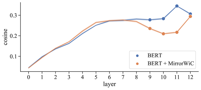
(e) BERT random-word cosine similarity

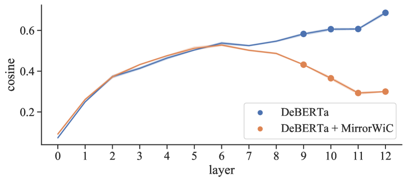
(f) DeBERTa random-word cosine similarity

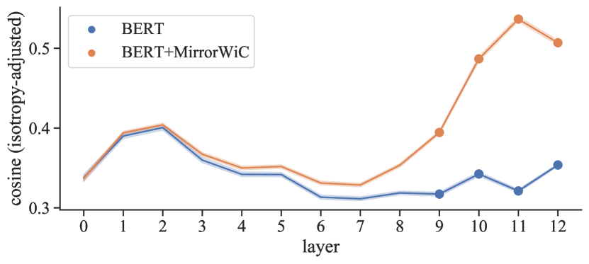
(g) BERT intra-sentence cosine similarity

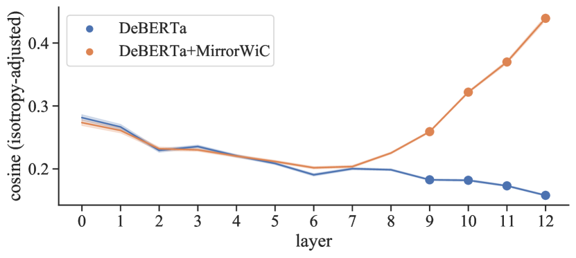
(h) DeBERTa intra-sentence cosine similarity

Figure 2: Layer-wise analyses of BERT (left column) and DeBERTA (right column) before and after applying MirrorWiC. The first row (a,b) shows the model performance and can be linked to the isotropy analysis (the middle two rows: c,d,e,f) and contextualisation analysis (the last row: g,b). Task performance correlates strongly with isotropy and contextualisation changes especially in the last four layers (highlighted with dots); shade=variance.

Impact of the Underlying PLM (Table 3). MirrorWiC is effective with BERT, RoBERTa and DeBERTa. DeBERTa+MirrorWiC yields larger gains, and even results in the highest absolute scores on average. In other words, a seemingly ‘weaker’ off-the-shelf PLM under the naive feature extraction baseline (DeBERTa) is transformed into the best-performing WiC encoder after the MirrorWiC procedure. This hints at the necessity to unlock the input PLM’s ’task solving potential’ through adaptive fine-tuning.

Comparison with Sentence Encoders (Table 3). We also probe how modelling the sentences (without knowing which target word the context is describing) performs on the evaluation tasks. In particular, we evaluate the standard ’go-to’ sentence encoder Sentence-BERT (Reimers and Gurevych, 2019b), and the original MirrorBert (Liu et al., 2021b). We find that MirrorWiC, with its direct focus on word-in-context representations and WiC-oriented fine-tuning, substantially outperforms the two sentence encoders. The finding validates our hypothesis that naively applying sentence encoders is not sufficient for context-aware lexical semantic tasks. While the two sentence encoders do provide competitive performance in WiC-style tasks, their performance decreases drastically on Usim. This further indicates that the fine-grained similarity-based Usim evaluation requires a more accurate and subtler contextual lexical semantic ability than the binary classification in WiC.

Comparison with Supervised WiC Methods (Table 4). The scores reveal that the unsupervised BERT + MirrorWiC variant can even outperform the supervised model (fine-tuned with labelled in-task data) in the WiC task. The results on TSV indicate that the gap between the unsupervised BERT-based approach to the supervised performance is much reduced: from the $\sim$10% gap to only $\sim$2% in all three TSV tasks when MirrorWiC is applied.

5.2 Multilingual and Cross-Lingual Results

The results are summarised in Table 5. Notably, we observe that the effectiveness of MirrorWiC is not tied to English, and extends to other languages. We observe consistent improvements with the underlying PLMs monolingually pretrained in other languages, as well as with the multilingually pretrained mBERT. The gains on XL-WiC are more pronounced than on the more difficult AM2iCo benchmark. By design AM2iCo is a more challenging benchmark, and additional external knowledge injection might be necessary to improve the results further; unlike XL-WiC, AM2ico requires the models to understand the cross-lingual correspondence of mostly entity names that occur less frequently.

model$\downarrow$, dataset$\rightarrow$	WiC	TSV-1	TSV-2	TSV-3
BERT	65.85	65.08	62.09	63.16
+ MirrorWiC	69.64	73.66	69.83	73.73
task-supervised BERT	69.00	75.30	71.40	76.60

Table 4: BERT+MirrorWiC versus supervised BERT-based methods on the test sets of English WiC-style tasks. The supervised variant on WiC is replicated from Wang et al. (2019). The supervised results on TSV are taken from Breit et al. (2021).

XL-WiC	zh *	ko *	hr	et
BERT	73.74	68.41	61.10	57.06
+ MirrorWiC	75.70	72.26	67.32	61.43
AM2iCo	zh	ka	ja	ar
BERT	63.80	59.90	64.10	60.60
+ MirrorWiC	64.60	61.00	64.70	63.90

Table 5: Results (test set accuracy) on multilingual and cross-lingual word-in-context tasks. We use mBERT as the underlying PLM for all the languages except for zh * and ko * (in XL-WiC) where their monolingual BERT models were used.

5.3 Further Discussion and Analyses

Layer-wise Performance (Figures 2(a) and 2(b)). The figures reveal that the success of MirrorWiC is attributed to the performance gains achieved in the last four layers of the fine-tuned PLMs. This is expected as these four layers are exactly what we optimise in the MirrorWiC procedure. This also confirms our hypothesis that matching training and inference representations helps adapt and elicit word-in-context knowledge from the PLMs.

Isotropy (Figures 2(c) and 2(d)). As empirically validated in prior work on sentence representations Gao et al. (2021); Liu et al. (2021b), contrastive fine-tuning reshapes the embedding space geometry towards more isotropic representations, which in turn has a positive impact on semantic similarity tasks. We now examine whether the same ‘isotropy-increasing’ effect is achieved with MirrorWiC. To this end, we leverage a quantitative isotropy score (IS), proposed in prior work (Arora et al., 2016; Mu and Viswanath, 2018), and defined as:

$$\text{IS}(\mathcal{V})=\log\left(\frac{\min_{\mathbf{c}\in\mathcal{C}}\sum_{\mathbf{v}\in\mathcal{V}}\exp(\mathbf{c}^{\top}\mathbf{v})}{\max_{\mathbf{c}\in\mathcal{C}}\sum_{\mathbf{v}\in\mathcal{V}}\exp(\mathbf{c}^{\top}\mathbf{v})}\right)$$ (2)

where $\mathcal{V}$ is the set of vectors, $\mathcal{C}$ is the set of all possible unit vectors in the embedding space (i.e., $\{\mathbf{c}:|\mathbf{c}|=1\}$). Practically, $\mathcal{C}$ is approximated by the eigenvector set of $\mathbf{V}^{\top}\mathbf{V}$ ($\mathbf{V}$ is the stacked embeddings of $\mathcal{V}$). The larger the IS value, the more isotropic an embedding space is.

As seen in Figure 2(c) and Figure 2(d), both BERT and DeBERTa create more isotropic embedding spaces in general in the last four layers after MirrorWiC training. Note that DeBERTa’s space isotropy is able to benefit more from MirrorWiC, which also explains its large gains in the end tasks.

It is also possible to assess isotropy by simply looking at the cosine similarity of random words Ethayarajh (2019). We calculate word representations in each layer as the average of the word’s contextual representations from Wikipedia. We then take five random samples of 200 random words and compute pair-wise similarity. We take the average of the similarity scores in each sample with variance reported in Figure 2(e) and Figure 2(f). The results confirm the trend: the last four layers with MirrorWiC exhibit much lower random word cosine similarities than the off-the-shelf PLM.

Word-in-context 1	Word-in-context 2	BERT	+MirrorWiC	Gold
Spend money.	He spends far more on gambling than he does on living proper.	-0.0850 (F)	0.2327 (T)	T
That toaster can make wonderful toasts.	I ate a piece of toast for breakfast.	0.0160 (F)	0.3234 (T)	T
War is hell.	The hell of battle.	-0.0403 (F)	0.2378 (T)	F
Ease the pain in your legs.	The pain eased overnight.	0.0157 (F)	0.2873 (T)	F

Table 6: Examples of changed cosine similarity scores (isotropy-adjusted) after MirrorWiC; English WiC (dev).

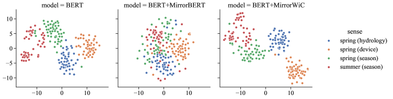
Figure 3: t-SNE embedding visualisation of different senses of spring and summer under different models.

Intra-Sentence Similarity (Figures 2(g) and 2(h)). As a measure of contextualisation, we follow Ethayarajh (2019), and define intra-sentence similarity as each word’s similarity to its context. The context is computed as the mean vector of all the word representations in the sentence. The scores are isotropy-adjusted by substracting the intra-sentence similarity scores by the random word similarity in each layer, see Ethayarajh (2019). For both BERT and DeBERTa, we can see that the last four layers become more contextualised after applying MirrorWiC: they encode more information about the context as the contextual word representations become much more similar to its context in the top Transformer layers than in the base PLM. This increased contextualisation could explain why MirrorWiC gives better performance in the context-sensitive lexical semantic tasks.

Error Analysis (Table 6). Conducting an error analysis of BERT before and after MirrorWiC on the WiC dev set, we observe that 94 instances changed their labels, among which 58 are MirrorWiC correcting the original predictions. In 43 out of 58 cases, MirrorWiC is producing more TRUE positives. The examples with the largest similarity changes are provided in the upper half of Table 6. For the 36 cases where MirrorWiC changes the originally correct predictions to the wrong prediction, 29 are false positives; see the lower half of Table 6. We manually inspect these cases and find that the distinctions between the two contexts are usually too fine-grained to tell even for humans. For instance, it seems acceptable to align with the MirrorWiC’s (incorrect) predictions for hell and ease in the two examples in Table 6.

Visualising the Embedding Space (Figure 3). Contextualised embeddings for an ambiguous word (spring) with off-the-shelf BERT, MirrorBert and MirrorWiC are visualised in Figure 3 (sense labels from Wikipedia). While MirrorWiC maintains the sense clusters from BERT and teases apart the different senses even more, MirrorBert exhibits no clear sense distinctions. This shows a fundamental difference between MirrorWiC and MirrorBert: MirrorBert is insensitive to the target word, and directly applying it to context-sensitive lexical tasks yields subpar performance.

5.4 Ablation Study

An ablation study is conducted on English WiC (dev). Foreshadowing, the dropout rate and the layer averaging strategy are the two most important factors for MirrorWiC to be effective.

Dropout and Random Span Masking (Tables 7 and 8). The MirrorWiC performance is most sensitive to the dropout rate; it requires larger dropout rates (0.3 for DeBERTa and 0.4 for BERT) than MirrorBert (0.1 dropout). This may be related to the different levels of granularity. Sentence meanings can largely change with even slight differences in context: therefore, positive sentence pairs for MirrorBert are required to be very similar. Word-in-context meaning can tolerate larger contextual differences: larger dropout rates are thus preferable with MirrorWiC to create positive pairs with more distinct representations. Random span masking is less crucial than the dropout rate, and gives only slight gains (Table 8).

Layer Averaging Strategy (Table 9). Averaging across all layers of the PLM is suboptimal for WiC representations, and the strategy of averaging only over the last four layers is indeed the optimal one for BERT. However, DeBERTa reaches its peak when averaging over the last 2 layers. Our findings corroborate those from previous studies which report that contextualised information is usually stored in higher layers Ethayarajh (2019); Garí Soler and Apidianaki (2021), and the bulk of decontextualised information is stored in lower layers Vulić et al. (2020).

Input Size (Figure 4). As in Figure 4, we show a sharp increase of performance from 5k to 10k on both Usim and WiC. While WiC maintains its performance with small fluctuation from 10k throughout to 50k, there is a clear downward slope for Usim from 10k onward. This is in line with findings in MirrorBert, and also shows that the model does not require plenty of fine-tuning data to transform into a WiC encoder. This further confirms that the model is not so much learning new knowledge as rewiring knowledge to the surface.

dropout rate$\rightarrow$	0	0.1	0.2	0.3	0.4	0.5	0.6
BERT + MirrorWiC	68.02	68.65	70.21	71.31	71.94	68.80	68.49
DeBERTa + MirrorWiC	65.67	69.12	70.53	71.78	67.08	65.98	66.30

Table 7: Impact of dropout rate in MirrorWiC.

model$\downarrow$, random span masking$\rightarrow$	off	on
BERT + MirrorWiC	71.31	71.47↑0.16
DeBERTa + MirrorWiC	71.78	71.94↑0.16

Table 8: Impact of random span masking.

average last $n$ layers$\rightarrow$	1	2	3	4	5	6	12
BERT + MirrorWiC	68.96	68.80	70.06	71.94	70.68	70.84	67.71
DeBERTa + MirrorWiC	71.47	73.04	72.41	71.78	71.15	70.53	69.74

Table 9: Impact of layer averaging strategies.

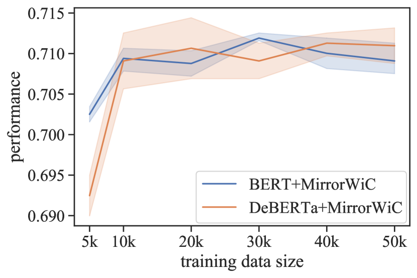
(a) WiC (dev)

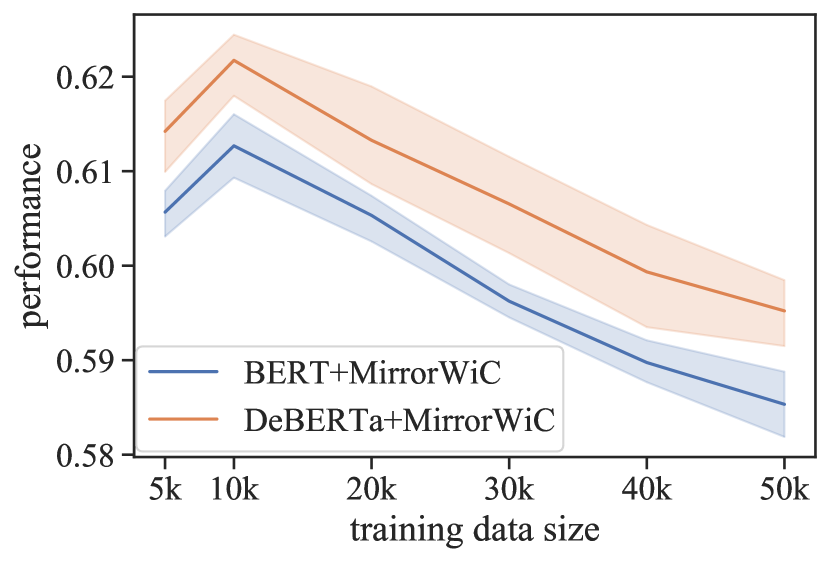
(b) Usim

Figure 4: Impact of input size of the training data for MirrorWiC. Evaluation on WiC (dev).

6 Conclusion

We proposed MirrorWiC, a fully unsupervised approach for eliciting word-in-context representations from pretrained language models (PLMs), requiring only raw sentences as input, and disposing of labelled data and sense inventories. We showed that MirrorWiC is PLM-agnostic and language-agnostic, yielding substantial performance boosts in context-aware lexical semantic tasks in English, multilingual and cross-lingual setups and demonstrating that additional WiC knowledge can be exposed from the PLMs. We then delved into the inner-working of MirrorWiC, demonstrating that the performance improvement strongly correlates with metrics such as isotropy score and intra-sentence word similarity. In future work, we will also look into weakly supervised approaches that combine self-supervision with external sense-related knowledge.

Appendix A Appendix

A.1 AUC Score Tables for Binary Classification Tasks

model$\downarrow$, dataset$\rightarrow$	WiC	TSV-1	TSV-2	TSV-3
Sentence-BERT	64.20	63.99	61.81	66.01
MirrorBert	67.31	70.53	68.00	70.28
BERT	71.61	62.06	59.48	61.45
+ MirrorWiC	74.89	72.10	67.92	73.03
DeBERTa	70.58	62.11	60.51	63.25
+ MirrorWiC	76.70	75.44	71.24	75.64

Table 10: AUC results for English tasks.

level$\rightarrow$	XL-WiC					AM2iCo
model$\downarrow$, language$\rightarrow$	zh *	ko *	hr	et		zh	ka	ja	ar
BERT	80.97	75.17	67.79	62.72		68.06	64.50	69.32	68.98
+ MirrorWiC	83.39	80.44	76.80	64.62		69.23	65.57	72.86	69.27

Table 11: AUC results for multilingual and cross-lingual tasks.

Following prior work, we reported accuracy in the main text. However, the threshold for TRUE/FALSE classification needs to be tuned on dev set. We thus report the AUC scores in Tables 10 and 11 which does not require tuning of any hyperparameter. The AUC scores demonstrate the same trend as accuracy scores.

A.2 Pretrained Encoders Details

For a full listing of HuggingFace model links and number of parameters for each model, see Table 12.

model	#param	URL
BERT	110M	https://huggingface.co/bert-base-uncased
RoBERTa	110M	https://huggingface.co/roberta-base
DeBERTa	138M	https://huggingface.co/microsoft/deberta-base
mBERT	168M	https://huggingface.co/bert-base-multilingual-uncased
BERT (zh)	103M	https://huggingface.co/bert-base-chinese
BERT (ko)	118M	https://huggingface.co/kykim/bert-kor-base

Table 12: A listing of HuggingFace URLs of all pretrained models used in this work.

A.3 Hyperparameter Optimisation

Table 13 shows a full listing of the hyperparameters (and their search space). As said in main text, hyperparameters remain as the same as set in prior work of Liu et al. (2021b), except for random span masking rate and dropout rate.

hyperparameters	search space
learning rate	{1e-5, 2e-5∗,3e-5}
batch size	200
training epochs	{1∗, 2, 3, 4}
training data size	{5k, 10k∗, 20k, 30k, 40k, 50k}
max_seq_length of tokeniser	50
$\tau$ in Equation 1	{0.02, 0.03, 0.04∗, 0.05, 0.06}
random span masking rate (BERT)	{0, 1, 5, 10∗, 15}
random span masking rate (RoBERTa)	{0∗, 1, 5, 10 15}
random span masking rate (DeBERTa)	{0, 1∗, 5, 10, 15}
dropout rate (BERT)	{0.1, 0.2, 0.3, 0.4∗, 0.5, 0.6}
dropout rate (RoBERTa)	{0.1, 0.2, 0.3∗, 0.4, 0.5, 0.6}
dropout rate (DeBERTa)	{0.1, 0.2, 0.3∗, 0.4, 0.5, 0.6}

Table 13: Hyperparameters along with their search grid. $\ast$ marks the values used to obtain the reported results. The hparams without any defined search grid are adopted directly from Liu et al. (2021a).

A.4 Sensitivity to Training Corpora

To test the robustness of the model to different corpora, we individually sampled five sets of 10k raw sentences and found only minor difference when fine-tuning on them ($\approx 0.003$ standard deviation for BERT +MirrorWiC and $\approx 0.001$ for DeBERTa +MirrorWiC). We also tested with fine-tuning with strictly ‘in-domain’ data, i.e., raw sentences (w/o labels) sampled from the training sets of WiC tasks, but found no substantial difference when comparing to fine-tuning on Wikipedia texts.

A.5 Software and Hardware Dependencies

Our experiments are implemented with PyTorch and Huggingface Transformers. For PyTorch training, Automatic Mixed Precision (AMP) is turned on. The hardware configuration is listed in Table 14. MirrorWiC training on this machine takes $\approx 30$ seconds.

hardware	specification
RAM	128 GB
CPU	AMD Ryzen 9 3900x 12-core processor × 24
GPU	NVIDIA GeForce RTX 2080 Ti (11 GB) $\times$ 2

Table 14: Hardware specifications of the used machine.

References

- Armendariz et al. (2020) Carlos Santos Armendariz, Matthew Purver, Matej Ulčar, Senja Pollak, Nikola Ljubešić, and Mark Granroth-Wilding. 2020. CoSimLex: A resource for evaluating graded word similarity in context. In Proceedings of the 12th Language Resources and Evaluation Conference, pages 5878–5886, Marseille, France. European Language Resources Association.
- Arora et al. (2016) Sanjeev Arora, Yuanzhi Li, Yingyu Liang, Tengyu Ma, and Andrej Risteski. 2016. A latent variable model approach to PMI-based word embeddings. Transactions of the Association for Computational Linguistics, 4:385–399.
- Blevins and Zettlemoyer (2020) Terra Blevins and Luke Zettlemoyer. 2020. Moving down the long tail of word sense disambiguation with gloss informed bi-encoders. In Proceedings of the 58th Annual Meeting of the Association for Computational Linguistics, pages 1006–1017, Online. Association for Computational Linguistics.
- Breit et al. (2021) Anna Breit, Artem Revenko, Kiamehr Rezaee, Mohammad Taher Pilehvar, and Jose Camacho-Collados. 2021. WiC-TSV: An evaluation benchmark for target sense verification of words in context. In Proceedings of the 16th Conference of the European Chapter of the Association for Computational Linguistics: Main Volume, pages 1635–1645, Online. Association for Computational Linguistics.
- Camacho-Collados and Pilehvar (2018) Jose Camacho-Collados and Mohammad Taher Pilehvar. 2018. From word to sense embeddings: A survey on vector representations of meaning. Journal of Artificial Intelligence Research, 63:743–788.
- Camacho-Collados et al. (2016) José Camacho-Collados, Mohammad Taher Pilehvar, and Roberto Navigli. 2016. Nasari: Integrating explicit knowledge and corpus statistics for a multilingual representation of concepts and entities. Artificial Intelligence, 240:36–64.
- Carlsson et al. (2021) Fredrik Carlsson, Amaru Cuba Gyllensten, Evangelia Gogoulou, Erik Ylipää Hellqvist, and Magnus Sahlgren. 2021. Semantic re-tuning with contrastive tension. In International Conference on Learning Representations.
- Chen et al. (2014) Xinxiong Chen, Zhiyuan Liu, and Maosong Sun. 2014. A unified model for word sense representation and disambiguation. In Proceedings of the 2014 Conference on Empirical Methods in Natural Language Processing (EMNLP), pages 1025–1035, Doha, Qatar. Association for Computational Linguistics.
- Devlin et al. (2019) Jacob Devlin, Ming-Wei Chang, Kenton Lee, and Kristina Toutanova. 2019. BERT: Pre-training of deep bidirectional transformers for language understanding. In Proceedings of the 2019 Conference of the North American Chapter of the Association for Computational Linguistics: Human Language Technologies, Volume 1 (Long and Short Papers), pages 4171–4186, Minneapolis, Minnesota. Association for Computational Linguistics.
- Erk et al. (2013) Katrin Erk, Diana McCarthy, and Nicholas Gaylord. 2013. Measuring word meaning in context. Computational Linguistics, 39(3):511–554.
- Ethayarajh (2019) Kawin Ethayarajh. 2019. How contextual are contextualized word representations? comparing the geometry of BERT, ELMo, and GPT-2 embeddings. In Proceedings of the 2019 Conference on Empirical Methods in Natural Language Processing and the 9th International Joint Conference on Natural Language Processing (EMNLP-IJCNLP), pages 55–65, Hong Kong, China. Association for Computational Linguistics.
- Feng et al. (2020) Fangxiaoyu Feng, Yinfei Yang, Daniel Cer, Naveen Arivazhagan, and Wei Wang. 2020. Language-agnostic BERT sentence embedding. CoRR, abs/2007.01852.
- Gao et al. (2021) Tianyu Gao, Xingcheng Yao, and Danqi Chen. 2021. Simcse: Simple contrastive learning of sentence embeddings. arXiv preprint arXiv:2104.08821.
- Garí Soler and Apidianaki (2021) Aina Garí Soler and Marianna Apidianaki. 2021. Let’s play mono-poly: Bert can reveal words’ polysemy level and partitionability into senses. Transactions of the Association for Computational Linguistics (TACL).
- Garí Soler et al. (2019) Aina Garí Soler, Anne Cocos, Marianna Apidianaki, and Chris Callison-Burch. 2019. A comparison of context-sensitive models for lexical substitution. In Proceedings of the 13th International Conference on Computational Semantics - Long Papers, pages 271–282, Gothenburg, Sweden. Association for Computational Linguistics.
- Hadiwinoto et al. (2019) Christian Hadiwinoto, Hwee Tou Ng, and Wee Chung Gan. 2019. Improved word sense disambiguation using pre-trained contextualized word representations. In Proceedings of the 2019 Conference on Empirical Methods in Natural Language Processing and the 9th International Joint Conference on Natural Language Processing (EMNLP-IJCNLP), pages 5297–5306, Hong Kong, China. Association for Computational Linguistics.
- He et al. (2020) Pengcheng He, Xiaodong Liu, Jianfeng Gao, and Weizhu Chen. 2020. Deberta: Decoding-enhanced bert with disentangled attention. arXiv preprint arXiv:2006.03654.
- Kim et al. (2021) Taeuk Kim, Kang Min Yoo, and Sang-goo Lee. 2021. Self-guided contrastive learning for BERT sentence representations. In Proceedings of the 59th Annual Meeting of the Association for Computational Linguistics and the 11th International Joint Conference on Natural Language Processing (Volume 1: Long Papers), pages 2528–2540, Online. Association for Computational Linguistics.
- Levine et al. (2020) Yoav Levine, Barak Lenz, Or Dagan, Ori Ram, Dan Padnos, Or Sharir, Shai Shalev-Shwartz, Amnon Shashua, and Yoav Shoham. 2020. SenseBERT: Driving some sense into BERT. In Proceedings of the 58th Annual Meeting of the Association for Computational Linguistics, pages 4656–4667, Online. Association for Computational Linguistics.
- Liu et al. (2021a) Fangyu Liu, Ehsan Shareghi, Zaiqiao Meng, Marco Basaldella, and Nigel Collier. 2021a. Self-alignment pretraining for biomedical entity representations. In Proceedings of the 2021 Conference of the North American Chapter of the Association for Computational Linguistics: Human Language Technologies. Association for Computational Linguistics.
- Liu et al. (2021b) Fangyu Liu, Ivan Vulić, Anna Korhonen, and Nigel Collier. 2021b. Fast, effective and self-supervised: Transforming masked language models into universal lexical and sentence encoders. arXiv preprint arXiv:2104.08027.
- Liu et al. (2020) Qianchu Liu, Diana McCarthy, and Anna Korhonen. 2020. Towards better context-aware lexical semantics:adjusting contextualized representations through static anchors. In Proceedings of the 2020 Conference on Empirical Methods in Natural Language Processing (EMNLP), pages 4066–4075, Online. Association for Computational Linguistics.
- Liu et al. (2021c) Qianchu Liu, Edoardo M Ponti, Diana McCarthy, Ivan Vulić, and Anna Korhonen. 2021c. Am2ico: Evaluating word meaning in context across low-resource languages with adversarial examples. arXiv preprint arXiv:2104.08639.
- Liu et al. (2019) Yinhan Liu, Myle Ott, Naman Goyal, Jingfei Du, Mandar Joshi, Danqi Chen, Omer Levy, Mike Lewis, Luke Zettlemoyer, and Veselin Stoyanov. 2019. Roberta: A robustly optimized bert pretraining approach. arXiv preprint arXiv:1907.11692.
- Loshchilov and Hutter (2019) Ilya Loshchilov and Frank Hutter. 2019. Decoupled weight decay regularization. In 7th International Conference on Learning Representations, ICLR 2019, New Orleans, LA, USA, May 6-9, 2019. OpenReview.net.
- Loureiro and Jorge (2019) Daniel Loureiro and Alípio Jorge. 2019. Language modelling makes sense: Propagating representations through WordNet for full-coverage word sense disambiguation. In Proceedings of the 57th Annual Meeting of the Association for Computational Linguistics, pages 5682–5691, Florence, Italy. Association for Computational Linguistics.
- Mickus et al. (2020) Timothee Mickus, Denis Paperno, Mathieu Constant, and Kees van Deemter. 2020. What do you mean, BERT? In Proceedings of the Society for Computation in Linguistics 2020, pages 279–290, New York, New York. Association for Computational Linguistics.
- Mu and Viswanath (2018) Jiaqi Mu and Pramod Viswanath. 2018. All-but-the-top: Simple and effective postprocessing for word representations. In 6th International Conference on Learning Representations, ICLR 2018, Vancouver, BC, Canada, April 30 - May 3, 2018, Conference Track Proceedings. OpenReview.net.
- Navigli (2009) Roberto Navigli. 2009. Word sense disambiguation: A survey. ACM Computing Surveys, 41(2):1–69.
- Oord et al. (2018) Aaron van den Oord, Yazhe Li, and Oriol Vinyals. 2018. Representation learning with contrastive predictive coding. arXiv preprint arXiv:1807.03748.
- Pedinotti and Lenci (2020) Paolo Pedinotti and Alessandro Lenci. 2020. Don’t invite BERT to drink a bottle: Modeling the interpretation of metonymies using BERT and distributional representations. In Proceedings of the 28th International Conference on Computational Linguistics, pages 6831–6837, Barcelona, Spain (Online). International Committee on Computational Linguistics.
- Pilehvar and Camacho-Collados (2019) Mohammad Taher Pilehvar and Jose Camacho-Collados. 2019. WiC: the word-in-context dataset for evaluating context-sensitive meaning representations. In Proceedings of the 2019 Conference of the North American Chapter of the Association for Computational Linguistics: Human Language Technologies, Volume 1 (Long and Short Papers), pages 1267–1273, Minneapolis, Minnesota. Association for Computational Linguistics.
- Raganato et al. (2017) Alessandro Raganato, José Camacho-Collados, and Roberto Navigli. 2017. Word sense disambiguation: A unified evaluation framework and empirical comparison. In Proceedings of EACL 2017, pages 99–110.
- Raganato et al. (2020) Alessandro Raganato, Tommaso Pasini, Jose Camacho-Collados, and Mohammad Taher Pilehvar. 2020. XL-WiC: A multilingual benchmark for evaluating semantic contextualization. In Proceedings of the 2020 Conference on Empirical Methods in Natural Language Processing (EMNLP), pages 7193–7206, Online. Association for Computational Linguistics.
- Rajaee and Pilehvar (2021) Sara Rajaee and Mohammad Taher Pilehvar. 2021. A cluster-based approach for improving isotropy in contextual embedding space. In Proceedings of the 59th Annual Meeting of the Association for Computational Linguistics and the 11th International Joint Conference on Natural Language Processing (Volume 2: Short Papers), pages 575–584, Online. Association for Computational Linguistics.
- Reif et al. (2019) Emily Reif, Ann Yuan, Martin Wattenberg, Fernanda B. Viégas, Andy Coenen, Adam Pearce, and Been Kim. 2019. Visualizing and measuring the geometry of BERT. In Advances in Neural Information Processing Systems 32: Annual Conference on Neural Information Processing Systems 2019, NeurIPS 2019, December 8-14, 2019, Vancouver, BC, Canada, pages 8592–8600.
- Reimers and Gurevych (2019a) Nils Reimers and Iryna Gurevych. 2019a. Sentence-BERT: Sentence embeddings using Siamese BERT-networks. In Proceedings of the 2019 Conference on Empirical Methods in Natural Language Processing and the 9th International Joint Conference on Natural Language Processing (EMNLP-IJCNLP), pages 3982–3992, Hong Kong, China. Association for Computational Linguistics.
- Reimers and Gurevych (2019b) Nils Reimers and Iryna Gurevych. 2019b. Sentence-BERT: Sentence embeddings using Siamese BERT-networks. In Proceedings of the 2019 Conference on Empirical Methods in Natural Language Processing and the 9th International Joint Conference on Natural Language Processing (EMNLP-IJCNLP), pages 3982–3992, Hong Kong, China. Association for Computational Linguistics.
- Ruder (2021) Sebastian Ruder. 2021. Recent advances in language model fine-tuning. http://ruder.io/recent-advances-lm-fine-tuning.
- Vulić et al. (2020) Ivan Vulić, Edoardo Maria Ponti, Robert Litschko, Goran Glavaš, and Anna Korhonen. 2020. Probing pretrained language models for lexical semantics. In Proceedings of the 2020 Conference on Empirical Methods in Natural Language Processing (EMNLP), pages 7222–7240, Online. Association for Computational Linguistics.
- Wang et al. (2019) Alex Wang, Yada Pruksachatkun, Nikita Nangia, Amanpreet Singh, Julian Michael, Felix Hill, Omer Levy, and Samuel R. Bowman. 2019. Superglue: A stickier benchmark for general-purpose language understanding systems. In Advances in Neural Information Processing Systems 32: Annual Conference on Neural Information Processing Systems 2019, NeurIPS 2019, December 8-14, 2019, Vancouver, BC, Canada, pages 3261–3275.
- Wiedemann et al. (2019) Gregor Wiedemann, Steffen Remus, Avi Chawla, and Chris Biemann. 2019. Does bert make any sense? interpretable word sense disambiguation with contextualized embeddings. arXiv preprint arXiv:1909.10430.
- Xu et al. (2020) Yige Xu, Xipeng Qiu, Ligao Zhou, and Xuanjing Huang. 2020. Improving bert fine-tuning via self-ensemble and self-distillation. arXiv preprint arXiv:2002.10345.
- Yan et al. (2021) Yuanmeng Yan, Rumei Li, Sirui Wang, Fuzheng Zhang, Wei Wu, and Weiran Xu. 2021. Consert: A contrastive framework for self-supervised sentence representation transfer. arXiv preprint arXiv:2105.11741.
- Zhang et al. (2021) Yan Zhang, Ruidan He, Zuozhu Liu, Lidong Bing, and Haizhou Li. 2021. Bootstrapped unsupervised sentence representation learning. In Proceedings of the 59th Annual Meeting of the Association for Computational Linguistics and the 11th International Joint Conference on Natural Language Processing (Volume 1: Long Papers), pages 5168–5180, Online. Association for Computational Linguistics.