Multiscale Manifold Warping

Abstract

Many real-world applications require aligning two temporal sequences, including bioinformatics, handwriting recognition, activity recognition, and human-robot coordination. Dynamic Time Warping (DTW) is a popular alignment method, but can fail on high-dimensional real-world data where the dimensions of aligned sequences are often unequal. In this paper, we show that exploiting the multiscale manifold latent structure of real-world data can yield improved alignment. We introduce a novel framework called Warping on Wavelets (WOW) that integrates DTW with a a multi-scale manifold learning framework called Diffusion Wavelets. We present a theoretical analysis of the WOW family of algorithms and show that it outperforms previous state of the art methods, such as canonical time warping (CTW) and manifold warping, on several real-world datasets.

1 Introduction

Figure 1: A real-word problem of aligning human motion from multimodal capture data (De la Torre et al., 2008) from the CMU Quality of Life Grand Challenge, which records human subjects cooking a variety of dishes. We propose a novel multiscale manifold framework to align such high dimensional time-series data.

Temporal alignment of time series is central to many real-world applications, including human motion recognition (see Figure 1) (Junejo et al., 2008), temporal segmentation (Zhou et al., 2008), modeling the spread of Covid-19 (Rojas et al., 2020), and building view-invariant representations of activities (Junejo et al., 2008). Dynamic time warping (DTW) (Sakoe and Chiba, 1978) is a widely-used classical approach to aligning time-series datasets. DTW requires an inter-set distance function, and often assumes both input data sets have the same dimensionality. DTW may also fail under arbitrary affine transformations of one or both inputs. Canonical time warping (CTW) (Zhou and De la Torre, 2009) combines DTW by with canonical correlation analysis (CCA) (Anderson, 2003) to find a joint lower-dimensional embedding of two time-series datasets, and subsequently align the datasets in the lower-dimensional space. However, CTW fails when the two related data sets require nonlinear transformations. Manifold warping (Vu et al., 2012)(Ham et al., 2005; Wang and Mahadevan, 2009) solved this by instead representing features in the latent joint manifold space of the sequences.

Prior manifold warping methods however do not exploit the multiscale nature of most datasets, which our proposed algorithms exploit. In this paper, we propose a novel variant of dynamic time warping that uses a type of multiscale wavelet analysis (Mallat, 1998) on graphs, called diffusion wavelets (Coifman and Maggioni, 2006) to address this gap. In particular, we develop a multiscale variant of manifold warping called WOW (warping on wavelets), and show that WOW outperforms several warping algorithms, including manifold warping, as well as two other novel warping methods.

2 Dynamic Time Warping

We give a brief review of dynamic time warping (Sakoe and Chiba, 1978). We are given two sequential data sets $X=[x_{1}^{T},\ldots,x_{n}^{T}]^{T}\in\mathbb{R}^{n\times d}$, $Y=[y_{1}^{T},\ldots,y_{m}^{T}]^{T}\in\mathbb{R}^{m\times d}$ in the same space with a distance function $dist:X\times Y\rightarrow\mathbb{R}$. Let $P=\{p_{1},...,p_{s}\}$ represent an alignment between $X$ and $Y$, where each $p_{k}=(i,j)$ is a pair of indices such that $x_{i}$ corresponds with $y_{j}$. Since the alignment is restricted to sequentially-ordered data, we impose the additional constraints:

$$p_{1} = (1,1)$$ (1)

$$p_{s} = (n,m)$$ (2)

$$p_{k+1}-p_{k} = (1,0)\>or\>(0,1)\>or\>(1,1)$$ (3)

A valid alignment must match the first and last instances and cannot skip any intermediate instance. Also, no two sub-alignments cross each other. We can also represent the alignment in matrix form $W$ where:

$$W_{i,j}=\left\{\begin{array}[]{ll}1&\mbox{if $(i,j)\in P$}\\ 0&\mbox{otherwise}\end{array}\right.$$ (4)

To ensure that $W$ represents an alignment which satisfies the constraints in Equations 1, 2, 3, $W$ must be in the following form: $W_{1,1}=1,W_{n,m}=1$, none of the columns or rows of $W$ is a $0$ vector, and there must not be any $0$ between any two $1$’s in a row or column of $W$. We call a $W$ which satifies these conditions a DTW matrix. An optimal alignment is the one which minimizes the loss function with respect to the DTW matrix $W$:

$$L_{\mbox{DTW}}(W)=\sum_{i,j}dist\left(x_{i},y_{j}\right)W_{i,j}$$ (5)

A naïve search over the space of all valid alignments would take exponential time; however, dynamic programming can produce an optimal alignment in $O(nm)$. When $m$ is high-dimensional, as in Figure 1, or if the two sequences have varying dimensionality, DTW is not as effective, and we turn next to discussing a broad framework to extend DTW based on exploiting the manifold nature of many real-world datasets.

3 Mutiscale Manifold Learning

Diffusion wavelets (DWT) (Coifman and Maggioni, 2006) extends the strengths of classical wavelets to data that lie on graphs and manifolds. The term diffusion wavelets is used because it is associated with a diffusion process that defines the different scales, allows a multiscale analysis of functions on manifolds and graphs.

The diffusion wavelet procedure is described in Figure 2. The main procedure is as follows: an input matrix $T$ is orthogonalized using an approximate $QR$ decomposition in the first step. $T$’s $QR$ decomposition is written as $T=QR$, where $Q$ is an orthogonal matrix and $R$ is an upper triangular matrix. The orthogonal columns of $Q$ are the scaling functions. They span the column space of matrix $T$. The upper triangular matrix $R$ is the representation of $T$ on the basis $Q$. In the second step, we compute $T^{2}$. Note this is not done simply by multiplying $T$ by itself. Rather, $T^{2}$ is represented on the new basis $Q$: $T^{2}=(RQ)^{2}$. Since $Q$ may have fewer columns than $T$, due to the approximate QR decomposition, $T^{2}$ may be a smaller square matrix. The above process is repeated at the next level, generating compressed dyadic powers $T^{2^{j}}$, until the maximum level is reached or its effective size is a $1\times 1$ matrix. Small powers of $T$ correspond to short-term behavior in the diffusion process and large powers correspond to long-term behavior.

$\{\phi_{j}$, $T_{j}\}=DWT(T,\phi_{0},QR,J,\varepsilon)$

INPUT:

$\,\,T$: Diffusion operator.

$\phi_{0}$: Initial basis matrix.

$QR$: A modified $QR$ decomposition.

$J$: Max step number

$\varepsilon$: Desired precision.

$\,\,//\textbf{OUTPUT}:\phi_{j}$: Diffusion scaling functions at scale $j$. $T_{j}=[T^{2^{j}}]_{\phi_{j}}^{\phi_{j}}$.

$For\,\,j=0\,\,\,to\,\,\,J-1$$\{$

$\,\,\,\,\,\,\,\,([\phi_{j+1}]_{\phi_{j}}$, $[T^{2^{j}}]_{\phi_{j}}^{\phi_{j+1}})\leftarrow QR([T^{2^{j}}]_{\phi_{j}}^{\phi_{j}},\varepsilon)$;

$\,\,\,\,\,\,\,\,[T^{2^{j+1}}]_{\phi_{j+1}}^{\phi_{j+1}}=([T^{2^{j}}]_{\phi_{j}}^{\phi_{j+1}}[\phi_{j+1}]_{\phi_{j}})^{2}$;

$\}$

Figure 2: Diffusion Wavelets construct multiscale representations at different scales. The notation $[T]_{\phi_{a}}^{\phi_{b}}$ denotes matrix $T$ whose column space is represented using basis $\phi_{b}$ at scale $b$, and row space is represented using basis $\phi_{a}$ at scale $a$. The notation $[{\phi_{b}}]_{\phi_{a}}$ denotes basis $\phi_{b}$ represented on the basis $\phi_{a}$. At an arbitrary scale $j$, we have $p_{j}$ basis functions, and length of each function is $l_{j}$. $[T]_{\phi_{a}}^{\phi_{b}}$ is a $p_{b}\times l_{a}$ matrix, $[{\phi_{b}}]_{\phi_{a}}$ is an $l_{a}\times p_{b}$ matrix.

An example of multiscale tree constructed by the diffusion wavelet procedure is shown in Figure 3, which is one of the real-world domains that we study later in the paper.

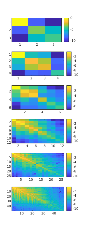
Figure 3: The diffusion wavelet procedure on a real-world CMU Quality of Life dataset (see Figure 1), where a subject is making brownies. The two sensor streams being aligned are an $87$-dimensional motion capture stream and a $11$-dimensional internal measurement unit system. The figure shows the diffusion wavelet tree constructed. The diffusion operator at each level is represented on the basis constructed at the previous level. The color values are scaled logarithmically.

We introduce multiscale Laplacian eigenmaps (Belkin and Niyogi, 2001a) and locality preserving projections (LPP) (He and Niyogi, 2003). Laplacian eigenmaps construct embeddings of data using the low-order eigenvectors of the graph Laplacian as a basis (Chung, 1997), which extends Fourier analysis to graphs and manifolds. Locality Preserving Projections (LPP) is a linear approximation of Laplacian eigenmaps. We review the multiscale Laplacian eigenmaps and multiscale LPP, based on the diffusion wavelets framework (Wang and Mahadevan, 2013b).

Notation: $X=[x_{1},\cdots,x_{n}]$ be an $p\times n$ matrix representing $n$ instances defined in a $p$ dimensional space. $W$ is an $n\times n$ weight matrix, where $W_{i,j}$ represents the similarity of $x_{i}$ and $x_{j}$ ($W_{i,j}$ can be defined by $e^{-\|x_{i}-x_{j}\|^{2}}$). $D$ is a diagonal valency matrix, where $D_{i,i}=\sum_{j}W_{i,j}$. $\mathcal{W}=D^{-0.5}WD^{-0.5}$. $\mathcal{L}=I-\mathcal{W}$, where $\mathcal{L}$ is the normalized Laplacian matrix and $I$ is an identity matrix. $XX^{T}=FF^{T}$, where $F$ is a $p\times r$ matrix of rank $r$. One way to compute $F$ from $X$ is singular value decomposition. $(\cdot)^{+}$ represents the Moore-Penrose pseudo inverse.
(1) Laplacian eigenmaps minimizes the cost function $\sum_{i,j}(y_{i}-y_{j})^{2}\mathcal{W}_{i,j}$, which encourages the neighbors in the original space to be neighbors in the new space. The $c$ dimensional embedding is provided by eigenvectors of $\mathcal{L}x=\lambda x$ corresponding to the $c$ smallest non-zero eigenvalues. The cost function for multiscale Laplacian eigenmaps is defined as follows: given $X$, compute $Y_{k}=[y_{k}^{1},\cdots,y_{k}^{n}]$ at level $k$ ($Y_{k}$ is a $p_{k}\times n$ matrix) to minimize $\sum_{i,j}(y_{k}^{i}-y_{k}^{j})^{2}\mathcal{W}_{i,j}$. Here $k=1,\cdots,J$ represents each level of the underlying manifold hierarchy.
(2) LPP is a linear approximation of Laplacian eigenmaps. LPP minimizes the cost function $\sum_{i,j}(f^{T}x_{i}-f^{T}x_{j})^{2}\mathcal{W}_{i,j}$, where the mapping function $f$ constructs a $c$ dimensional embedding, and is defined by the eigenvectors of $X\mathcal{L}X^{T}x=\lambda XX^{T}x$ corresponding to the $c$ smallest non-zero eigenvalues. Similar to multiscale Laplacian eigenmaps, multiscale LPP learns linear mapping functions defined at multiple scales to achieve multilevel decompositions.

3.1 The Multiscale Algorithms

1. Construct diffusion matrix $T$ characterizing the given data set: • $T=I-\mathcal{L}$ is an $n\times n$ diffusion matrix. 2. Construct multiscale basis functions using diffusion wavelets: • $\{\phi_{j},T_{j}\}=DWT(T,I,QR,J,\varepsilon)$. • The resulting $[\phi_{j}]_{\phi_{0}}$ is an $n\times p_{j}$ matrix (Equation (6)). 3. Compute lower dimensional embedding (at level $j$): • The embedding $x_{i}\rightarrow y_{i}=$ row $i$ of $[\phi_{j}]_{\phi_{0}}$.

1. Construct relationship matrix $T$ characterizing the given data set: • $T=(F^{+}X\mathcal{L}X^{T}(F^{T})^{+})^{+}$ is an $r\times r$ matrix.. 2. Apply diffusion wavelets to explore the intrinsic structure of the data: • $\{\phi_{j},T_{j}\}=DWT(T,I,QR,J,\varepsilon)$. • The resulting $[\phi_{j}]_{\phi_{0}}$ is an $r\times p_{j}$ matrix (Equation (6)). 3. Compute lower dimensional embedding (at level $j$): • The embedding $x_{i}\rightarrow y_{i}={((F^{T})^{+}[\phi_{j}]_{\phi_{0}})}^{T}x_{i}$.

Figure 4: Top: Multiscale Laplacian Eigenmaps; Bottom: Multiscale LPP.

Multiscale Laplacian eigenmaps and multiscale LPP algorithms are shown in Figure 4, where $[\phi_{j}]_{\phi_{0}}$ is used to compute a lower dimensional embedding. As shown in Figure 2, the scaling functions $[\phi_{j+1}]_{\phi_{j}}$ are the orthonormal bases that span the column space of $T$ at different levels. They define a set of new coordinate systems revealing the information in the original system at different scales. The scaling functions also provide a mapping between the data at longer spatial/temporal scales and smaller scales. Using the scaling functions, the basis functions at level $j$ can be represented in terms of the basis functions at the next lower level. In this manner, the extended basis functions can be expressed in terms of the basis functions at the finest scale using:

$$[\phi_{j}]_{\phi_{0}}=[\phi_{j}]_{\phi_{j-1}}[\phi_{j-1}]_{\phi_{0}}=[\phi_{j}]_{\phi_{j-1}}\cdots[\phi_{1}]_{\phi_{0}}[\phi_{0}]_{\phi_{0}},$$ (6)

where each element on the right hand side of the equation is created by the procedure shown in Figure 2. In our approach, $[\phi_{j}]_{\phi_{0}}$ is used to compute lower dimensional embeddings at multiple scales. Given $[\phi_{j}]_{\phi_{0}}$, any vector/function on the compressed large scale space can be extended naturally to the finest scale space or vice versa. The connection between vector $v$ at the finest scale space and its compressed representation at scale $j$ is computed using the equation $[v]_{\phi_{0}}=([\phi_{j}]_{\phi_{0}})[v]_{\phi_{j}}$. The elements in $[\phi_{j}]_{\phi_{0}}$ are usually much coarser and smoother than the initial elements in $[\phi_{0}]_{\phi_{0}}$, which is why they can be represented in a compressed form.

4 Multiscale Manifold Alignment

We describe a general framework for transfer learning across two datasets called manifold alignment (Ma and Fu, 2011; Wang and Mahadevan, 2009). We are given the data sets $X$ and $Y$ of shapes $N_{X}\times D_{X}$ and $N_{Y}\times D_{Y}$, where each row is a sample (or instance) and each column is a feature, and a correspondence matrix $C^{(X,Y)}$ of shape $N_{X}\times N_{Y}$, where

$$C_{i,j}^{(X,Y)}=\left\{\begin{array}[]{ll}1&:\text{$X_{i}$ is in correspondence with $Y_{j}$}\\ 0&:\text{otherwise}\end{array}\right..$$ (7)

Manifold alignment calculates the embedded matrices $F^{(X)}$ and $F^{(Y)}$ of shapes $N_{X}\times d$ and $N_{Y}\times d$ for $d\leq min(D_{X},D_{Y})$ that are the embedded representation of $X$ and $Y$ in a shared, low-dimensional space. These embeddings aim to preserve both the intrinsic geometry within each data set and the sample correspondences among the data sets. More specifically, the embeddings minimize the following loss function:

$$L_{\mbox{MA}}\left(F^{(X)},F^{(Y)}\right) =\frac{\mu}{2}\sum_{i=1}^{N_{X}}\sum_{j=1}^{N_{Y}}||F_{i}^{(X)}-F_{j}^{(Y)}||_{2}^{2}C_{i,j}^{(X,Y)}$$

$$+\frac{1-\mu}{2}\sum_{i,j=1}^{N_{X}}||F_{i}^{(X)}-F_{j}^{(X)}||_{2}^{2}W_{i,j}^{(X)}$$

$$+\frac{1-\mu}{2}\sum_{i,j=1}^{N_{Y}}||F_{i}^{(Y)}-F_{j}^{(Y)}||_{2}^{2}W_{i,j}^{(Y)},$$ (8)

where $N$ is the total number of samples $N_{X}+N_{Y}$, $\mu\in[0,1]$ is the correspondence tuning parameter, and $W^{(X)},W^{(Y)}$ are the calculated similarity matrices of shapes $N_{X}\times N_{X}$ and $N_{Y}\times N_{Y}$, such that

$$W_{i,j}^{(X)}=\left\{\begin{array}[]{ll}k(X_{i},X_{j})&:\text{$X_{j}$ is a neighbor of $X_{i}$}\\ 0&:\text{otherwise}\end{array}\right.$$ (9)

for a given kernel function $k(\cdot,\cdot)$. $W_{i,j}^{(Y)}$ is defined in the same fashion. Typically, $k$ is set to be the nearest neighbor set member function or the heat kernel
$k(X_{i},X_{j})=\exp{\left(-|X_{i}-X_{j}|^{2}\right)}$.

In the loss function of equation (4), the first term corresponds to the alignment error between corresponding samples in different data sets. The second and third terms correspond to the local reconstruction error for the data sets $X$ and $Y$ respectively. This equation can be simplified using block matrices by introducing a joint weight matrix $W$ and a joint embedding matrix $F$, where

$$W=\left[\begin{array}[]{cc}(1-\mu)W^{(X)}&\mu C^{(X,Y)}\\ \mu C^{(Y,X)}&(1-\mu)W^{(Y)}\end{array}\right]$$ (10)

and

$$F=\left[\begin{array}[]{c}F^{(X)}\\ F^{(Y)}\end{array}\right].$$ (11)

4.1 Multiscale alignment

Given a fixed sequence of dimensions, $d_{1}>d_{2}>\ldots>d_{h}$, as well as two datasets, $X$ and $Y$, and some partial correspondence information, $x_{i}\in X_{l}\longleftrightarrow y_{i}\in Y_{l}$,the multiscale manifold alignment problem is to compute mapping functions, $\mathcal{A}_{k}$ and $\mathcal{B}_{k}$, at each level $k$ ($k=1,2,\ldots,h$) that project $X$ and $Y$ to a new space, preserving local geometry of each dataset and matching instances in correspondence. Furthermore, the associated sequence of mapping functions should satisfy $span(\mathcal{A}_{1})\supseteq span(\mathcal{A}_{2})\supseteq\ldots\supseteq span(\mathcal{A}_{h})$ and $span(\mathcal{B}_{1})\supseteq span(\mathcal{B}_{2})\supseteq\ldots\supseteq span(\mathcal{B}_{h})$, where $span(\mathcal{A}_{i})$ (or $span(\mathcal{B}_{i})$)represents the subspace spanned by the columns of $\mathcal{A}_{i}$ (or $\mathcal{B}_{i}$).

To apply diffusion wavelets to the multiscale alignment problem, the construction needs to be able to handle two input matrices $A$ and $B$ that occur in a generalized eigenvalue decomposition, $A\gamma=\lambda B\gamma$. The following theoretical result shows how to carry out such an extension (Wang and Mahadevan, 2013a). Given $X,X_{l},Y,Y_{l}$, using the notation defined in Figure 5, the algorithm is given below as Algorithm 2.

1. Construct a matrix representing the joint manifold: $T=F^{+}ZLZ^{T}(F^{T})^{+}$.

2. Use diffusion wavelets on the joint manifold:

   $[\phi_{k}]_{\phi_{0}}=\mathcal{DWT}(T^{+},\epsilon)$, where $\mathcal{DWT()}$ is the diffusion wavelets algorithm.

3. Compute mapping functions for manifold alignment (at level $k$):

$\left[\begin{array}[]{c}\alpha_{k}\\ \beta_{k}\\ \end{array}\right]=(F^{T})^{+}[\phi_{k}]_{\phi_{0}}$ is a $(p+q)\times d_{k}$ matrix.

At level $k$: apply $\alpha_{k}$ and $\beta_{k}$ to find correspondences between $X$ and $Y$:

For any $i$ and $j$, $\alpha_{k}^{T}x_{i}$ and $\beta_{k}^{T}y_{j}$ are in the same $d_{k}$ dimensional space.

Algorithm 1 Multiscale Manifold Alignment (MMA)

$x_{i}\in R^{p}$; $X=\{x_{1},\cdots,x_{m}\}$ is a $p\times m$ matrix;

$X_{l}=\{x_{1},\cdots,x_{l}\}$ is a $p\times l$ matrix.

$y_{i}\in R^{q}$; $Y=\{y_{1},\cdots,y_{n}\}$ is a $q\times n$ matrix;

$Y_{l}=\{y_{1},\cdots,y_{l}\}$ is a $q\times l$ matrix .

$X_{l}$ and $Y_{l}$ are in correspondence: $x_{i}\in X_{l}\longleftrightarrow y_{i}\in Y_{l}$.

$W_{x}$ is a similarity matrix, e.g. $W_{x}^{i,j}=e^{-\frac{||x_{i}-x_{j}||^{2}}{2\sigma^{2}}}$.

$D_{x}$ is a full rank diagonal matrix: $D_{x}^{i,i}=\sum_{j}W_{x}^{i,j}$;

$L_{x}=D_{x}-W_{x}$ is the combinatorial Laplacian matrix.

$W_{y}$, $D_{y}$ and $L_{y}$ are defined similarly.

$\Omega_{1}-\Omega_{4}$ are all diagonal matrices having $\mu$ on the top $l$ elements

of the diagonal (the other elements are 0s);

$\Omega_{1}$ is an $m\times m$ matrix; $\Omega_{2}$ and $\Omega_{3}^{T}$ are $m\times n$ matrices;

$\Omega_{4}$ is an $n\times n$ matrix.

$Z=\left(\begin{array}[]{cc}X&0\\ 0&Y\\ \end{array}\right)$ is a $(p+q)\times(m+n)$ matrix.

$D=\left(\begin{array}[]{cc}D_{x}&0\\ 0&D_{y}\\ \end{array}\right)$ and $L=\left(\begin{array}[]{cc}L_{x}+\Omega_{1}&-\Omega_{2}\\ -\Omega_{3}&L_{y}+\Omega_{4}\\ \end{array}\right)$

are both $(m+n)\times(m+n)$ matrices.

$F$ is a $(p+q)\times r$ matrix, where $r$ is the rank of $ZDZ^{T}$

and $FF^{T}=ZDZ^{T}$. $F$ can be constructed by SVD.

$(\cdot)^{+}$ represents the Moore-Penrose pseudoinverse.

At level $k$: $\alpha_{k}$ is a mapping from $x\in X$ to a point,

$\alpha_{k}^{T}x$, in a $d_{k}$ dimensional space ($\alpha_{k}$ is a $p\times d_{k}$ matrix).

At level $k$: $\beta_{k}$ is a mapping from $y\in Y$ to a point,

$\beta_{k}^{T}y$, in a $d_{k}$ dimensional space

($\beta_{k}$ is a $q\times d_{k}$ matrix).

Figure 5: Notation used in this section.

Theorem 1.

The solution to the generalized eigenvalue decomposition $ZLZ^{T}\gamma=\lambda ZDZ^{T}\gamma$ is given by $((F^{T})^{+}x,\lambda)$, where $x$ and $\lambda$ are eigenvector and eigenvalue of $F^{+}ZLZ^{T}(F^{T})^{+}x=\lambda x$.

Proof: Using the notation summarized in Figure 5, $ZDZ^{T}=FF^{T}$, where $F$ is a $(p+q)\times r$ matrix of rank $r$ and can be constructed by singular value decomposition. It is obvious that $ZDZ^{T}$ is positive semi-definite.
Case 1: when $ZDZ^{T}$ is positive definite:
It can be seen that $r=p+q$. This implies that $F$ is a $(p+q)\times(p+q)$ full rank matrix: $F^{-1}=F^{+}$.
$ZLZ^{T}\gamma=\lambda ZDZ^{T}\gamma$ $\Longrightarrow ZLZ^{T}\gamma=\lambda FF^{T}\gamma$ $\Longrightarrow ZLZ^{T}\gamma=\lambda F(F^{T}\gamma)$
$\Longrightarrow ZLZ^{T}(F^{T})^{-1}(F^{T}\gamma)=\lambda F(F^{T}\gamma)$ $\Longrightarrow F^{-1}ZLZ^{T}(F^{T})^{-1}(F^{T}\gamma)=\lambda(F^{T}\gamma)$
$\Longrightarrow$ Solution to $ZLZ^{T}\gamma=\lambda ZDZ^{T}\gamma$ is given by $((F^{T})^{+}x,\lambda)$, where $x$ and $\lambda$ are eigenvector and eigenvalue of $F^{+}ZLZ^{T}(F^{T})^{+}x=\lambda x$.
Case 2: when $ZDZ^{T}$ is positive semi-definite but not positive definite:
In this case, $r<p+q$ and $F$ is a $(p+q)\times r$ matrix of rank $r$.
Since $ZD^{0.5}$ is a $(p+q)\times(m+n)$ matrix, $F$ is a $(p+q)\times r$ matrix, there exits a matrix $G$ such that $ZD^{0.5}=FG$. This implies $Z=FGD^{-0.5}$ and $GD^{-0.5}=F^{+}Z$.
$ZLZ^{T}\gamma=\lambda ZDZ^{T}\gamma$
$\Longrightarrow FGD^{-0.5}LD^{-0.5}G^{T}F^{T}\gamma=\lambda FF^{T}\gamma$ $\Longrightarrow FGD^{-0.5}LD^{-0.5}G^{T}(F^{T}\gamma)=\lambda F(F^{T}\gamma)$
$\Longrightarrow(F^{+}F)GD^{-0.5}LD^{-0.5}G^{T}(F^{T}\gamma)=\lambda(F^{T}\gamma)$
$\Longrightarrow GD^{-0.5}LD^{-0.5}G^{T}(F^{T}\gamma)=\lambda(F^{T}\gamma)$ $\Longrightarrow F^{+}ZLZ^{T}(F^{T})^{+}(F^{T}\gamma)=\lambda(F^{T}\gamma)$
$\Longrightarrow$ One solution to $ZLZ^{T}\gamma=\lambda ZDZ^{T}\gamma$ is $((F^{T})^{+}x,\lambda)$, where $x$ and $\lambda$ are eigenvector and eigenvalue of $F^{+}ZLZ^{T}(F^{T})^{+}x=\lambda x$. Note that eigenvector solution to Case 2 is not unique.

Theorem 2.

At level $k$, the multiscale manifold alignment algorithm achieves the optimal $d_{k}$ dimensional alignment result with respect to the cost function $C(\alpha,\beta)$.

Proof: Let $T=F^{+}ZLZ^{T}(F^{T})^{+}$. Since $L$ is positive semi-definite, $T$ is also positive semi-definite. This means all eigenvalues of $T\geq 0$, and eigenvectors corresponding to the smallest non-zero eigenvalues of $T$ are the same as the eigenvectors corresponding to the largest eigenvalues of $T^{+}$. From Theorem 1, we know the solution to generalized eigenvalue decomposition $ZLZ^{T}\gamma=\lambda ZDZ^{T}\gamma$ is given by $((F^{T})^{+}x,\lambda)$, where $x$ and $\lambda$ are eigenvector and eigenvalue of $Tx=\lambda x$. Let columns of $P_{X}$ denote the eigenvectors corresponding to the $d_{k}$ largest non-zero eigenvalues of $T^{+}$. Then the linear LPP-like solution is given by $(F^{T})^{+}P_{X}$.

Let columns of $P_{Y}$ denote $[\phi_{k}]_{\phi_{0}}$, the scaling functions of $T^{+}$ at level $k$ and $d_{k}$ be the number of columns of $[\phi_{k}]_{\phi_{0}}$. In our multiscale algorithm, the solution at level $k$ is provided by $(F^{T})^{+}P_{Y}$.

From (Coifman and Maggioni, 2006), we know $P_{X}$ and $P_{Y}$ span the same space. This means $P_{X}P_{X}^{T}=P_{Y}P_{Y}^{T}$. Since the columns of both $P_{X}$ and $P_{Y}$ are orthonormal, we have $P_{X}^{T}P_{X}=P_{Y}^{T}P_{Y}=I$, where $I$ is an $d_{k}$$\times$$d_{k}$ identity matrix. Let $Q=P_{Y}^{T}P_{X}$, then $P_{X}=P_{X}I=P_{X}P_{X}^{T}P_{X}=P_{Y}P_{Y}^{T}P_{X}=P_{Y}(P_{Y}^{T}P_{X})\Longrightarrow P_{X}=P_{Y}Q$.

$Q^{T}Q=QQ^{T}=I$ and $det(Q^{T}Q)=(det(Q))^{2}=1$, $det(Q)=1$. So $Q$ is a rotation matrix.

Combining the results shown above, the multiscale alignment algorithm at level $k$ and manifold projections with $d_{k}$ smallest non-zero eigenvectors achieve the same alignment results up to a rotation $Q$.∎

5 Multiscale Dynamic Time Warping

Input: X,Y: two time-series data sets

d: latent space dimension

$\mu,\tau$: hyper-parameters as described in Algorithm 3.

Output: $F^{(X)},F^{(Y)}$: the embeddings of X and Y in the latent space

$W^{(X,Y)}$: the result DTW matrix that provides the alignment of X and Y

begin

       $t\leftarrow 0$

       $F^{\left(X\right),t}\leftarrow\mbox{MLE}\left(X,\tau\right)$

       $F^{\left(Y\right),t}\leftarrow\mbox{MLE}\left(Y,\tau\right)$

       repeat

             $W=\left[\begin{array}[]{cc}(1-\mu)W^{(X)}&\mu W^{(X,Y),t}\\ \mu(W^{(X,Y),t})^{T}&(1-\mu)W^{(Y)}\end{array}\right]$

             $\phi^{(Y),t+1},\phi^{(X),t+1}$ $\leftarrow\mbox{MMA}\left(F^{\left(X\right),t},F^{\left(Y\right),t},W,d,\mu,\tau\right)$

             $F^{(X),t+1}\leftarrow F^{(X),t}\phi^{(X),t+1}$

             $F^{(Y),t+1}\leftarrow F^{(Y),t}\phi^{(Y),t+1}$

             $W^{\left(X,Y\right),t+1}\leftarrow\mbox{DTW}\left(F^{\left(X\right),t+1},F^{\left(Y\right),t+1}\right)$

             $t\leftarrow t+1$

      until convergence;

      $F^{(X)}\leftarrow F^{(X),t}$; $F^{(Y)}\leftarrow F^{(Y),t}$; $W^{(X,Y)}\leftarrow W^{(X,Y),t}$

end

Algorithm 2 Warping on Wavelets (WOW)

Algorithm 2 describes a novel multiscale diffusion-wavelet based framework for aligning two sequentially-ordered data sets. MLE denotes the multi-scale Laplacian Eigenmaps algorithm described in Figure 4. Also, MMA denotes the multi-scale manifold alignment method described in Section 4 as Algorithm 1. We reformulate the loss function for WOW as:

$$\begin{array}[]{l}L_{\mbox{WOW}}(\phi^{(X)},\phi^{(Y)},W^{(X,Y)})\\ =((1-\mu)\displaystyle\sum_{i,j\in X}||F_{i}^{(X)}\phi^{(X)}-F_{j}^{(X)}\phi^{(X)}||^{2}W_{i,j}^{(X)}\\ +(1-\mu)\displaystyle\sum_{i,j\in Y}||F_{i}^{(Y)}\phi^{(Y)}-F_{j}^{(Y)}\phi^{(Y)}||^{2}W_{i,j}^{(Y)}\\ +\mu\displaystyle\sum_{i\in X,j\in Y}||F_{i}^{(X)}\phi^{(X)}-F_{j}^{(Y)}\phi^{(Y)}||^{2}W_{i,j}^{(X,Y)})\end{array}$$ (12)

which is the same loss function as in linear manifold alignment except that $W^{(X,Y)}$ is now a variable.

Theorem 3.

Let $L_{\mbox{WOW},t}$ be the loss function $L_{\mbox{WOW}}$ evaluated at
$\prod_{i=1}^{t}\phi^{(X),i},\prod_{i=1}^{t}\phi^{(Y),i},W^{(X,Y),t}$ of Algorithm 2. The sequence $L_{\mbox{WOW},t}$ converges to a minimum as $t\rightarrow\infty$. Therefore, Algorithm 2 will terminate.

Proof: At any iteration $t$, Algorithm 2 first fixes the correspondence matrix at $W^{(X,Y),t}$. Now let $L_{\mbox{WOW}}^{\prime}$ equal $L_{\mbox{WOW}}$ above, except we replace $F_{i}^{(X)},F_{i}^{(Y)}$ by $F_{i}^{(X),t},F_{i}^{(Y),t}$ and Algorithm 2 minimizes over $\phi^{(X),t+1},\phi^{(Y),t+1}$ using mixed manifold alignment. Thus,

$$\begin{array}[]{l}L_{\mbox{WOW}}^{\prime}(\phi^{(X),t+1},\phi^{(Y),t+1},W^{(X,Y),t})\\ \leq L_{\mbox{WOW}}^{\prime}(I,I,W^{(X,Y),t})\\ =L_{\mbox{WOW}}(\prod_{i=1}^{t}\phi^{(X),i},\prod_{i=1}^{t}\phi^{(Y),i},W^{(X,Y),t})\\ =L_{\mbox{WOW},t}\end{array}$$ (13)

since $F^{(X),t}=F^{(X),0}\prod_{i=1}^{t}\phi^{(X),i}$ and $F^{(Y),t}=F^{(Y),0}\prod_{i=1}^{t}\phi^{(X),i}$. We also have:

$$\begin{array}[]{l}L_{\mbox{WOW}}^{\prime}(\phi^{(X),t+1},\phi^{(Y),t+1},W^{(X,Y),t})\\ =L_{\mbox{WOW}}(\prod_{i=1}^{t+1}\phi^{(X),i},\prod_{i=1}^{t+1}\phi^{(Y),i},W^{(X,Y),t})\\ \leq L_{\mbox{WOW},t}\end{array}$$ (14)

Algorithm 2 then performs DTW to change $W^{(X,Y),t}$ to $W^{(X,Y),t+1}$. Using the same argument as in the proof of Theorem 2, we have:

$$\begin{array}[]{l}L_{\mbox{WOW}}(\prod_{i=1}^{t+1}\phi^{(X),i},\prod_{i=1}^{t+1}\phi^{(Y),i},W^{(X,Y),t+1})\\ \leq L_{\mbox{WOW}}(\prod_{i=1}^{t+1}\phi^{(X),i},\prod_{i=1}^{t+1}\phi^{(Y),i},W^{(X,Y),t})\\ \leq L_{\mbox{WOW},t}\\ \Leftrightarrow L_{\mbox{WOW},t+1}\leq L_{\mbox{WOW},t}.\end{array}$$ (15)

6 Warping on Mixed Manifolds

We describe two additional novel variants of dynamic time warping, one called mixed-manifold warping (or WAMM), and the other called curve wrapping.

6.1 Low Rank Embedding of Datasets on Mixed Manifolds

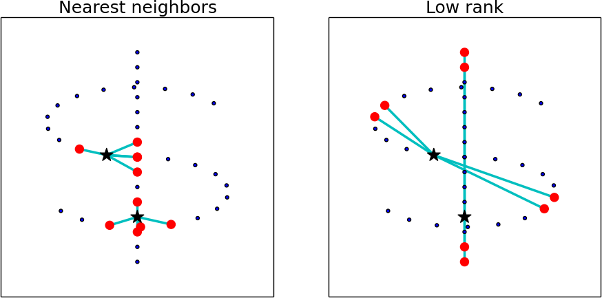
Figure 6: Manifold discovery is nontrivial when there are multiple intersecting manifolds on which the data potentially lies on. Popular manifold learning algorithms use nearest neighbor construction (on the left), which incorrectly creates short-circuits, whereas a low rank reconstruction (on the right) that correctly differentiates the mixed manifolds.

Traditional manifold learning methods, like LLE (Roweis and Saul, 2000) and Laplacian eigenmaps (Belkin and Niyogi, 2001b), construct a discretized approximation to the underlying manifold by constructing a nearest-neighbor graph of data points in the original high-dimensional space. When data lies on a more complex mixture of manifolds, methods that rely on nearest neighbor graph construction algorithms are thus prone to creating spurious inter-manifold connections when mixtures of manifolds are present. These so-called short-circuit connections are most commonly found at junction points between manifolds. Figure 6 shows an example of this phenomena using a noisy dollar sign data set.

To deal with complex intersecting manifolds, we describe an alternative approach that uses a low-rank reconstruction of the data points that correctly identifies points that lie on mixed manifolds (Favaro et al., 2011; Boucher et al., 2015a). Given a dataset $X$, the first step is to construct a low-rank approximation by reconstructing each point as a linear combination of the other data points. Unlike LLE, which uses a nearest-neighbor approach to manifold construction that is prone to short-circuit errors such as shown in Figure 6, our approach is based on a low-rank reconstruction matrix $R$ from minimizing the following objective function:

Input: X,Y: two time-series data sets

d: latent space dimension

k: number of nearest neighbors used

$\tau$: hyper-parameter for low-rank embedding

$\mu$: hyper-parameter preserving correspondence vs local geometry factor

Output: $F^{(X)},F^{(Y)}$: the embeddings of X and Y in the latent space

$W^{(X,Y)}$: the result DTW matrix that provides the alignment of X and Y

begin

       Set $W^{(X,Y)}_{1,1}=W^{(X,Y)}_{n_{X},n_{Y}}=1$, and $0$ everywhere else $t\leftarrow 0$

       repeat

             $W=\left[\begin{array}[]{cc}(1-\mu)W^{(X)}&\mu W^{(X,Y),t}\\ \mu(W^{(X,Y),t})^{T}&(1-\mu)W^{(Y)}\end{array}\right]$

             $F^{(X),t+1},F^{(Y),t+1}\leftarrow\mbox{MLE}(F^{(X),t},F^{(Y),t},W,d,\mu,\tau)$

             $W^{(X,Y),t+1}\leftarrow\mbox{DTW}(F^{(X),t+1},F^{(Y),t+1})$

             $t\leftarrow t+1$

      until convergence;

      $F^{(X)}\leftarrow F^{(X),t}$; $F^{(Y)}\leftarrow F^{(Y),t}$; $W^{(X,Y)}\leftarrow W^{(X,Y),t}$

end

Algorithm 3 Warping on Mixed Manifolds (WAMM)

In Algorithm 3, MLE(X,Y,W,d,$\mu$) is a function that returns the embedding of $X,Y$ in a $d$ dimensional space using (mixed) manifold alignment with the joint similarity matrix $W$ and parameter $\mu$ described in the previous sections. To construct such an embedding, we introduce the MME (for mixed-manifold) embedding objective function:

$$L_{\mbox{MLE}}(R,\tau)=\min_{R}\frac{1}{2}\frac{\tau}{2}||X-XR||_{F}^{2}+||R||_{*},$$ (16)

where $\lambda>0$, $||X||_{F}=\sqrt{\sum_{i}\sum_{j}|x_{i.j}|^{2}}$ is the Frobenius norm, and $||X||_{*}=\sum_{i}\sigma_{i}(X)$ is the spectral norm, for singular values $\sigma_{i}$.

(Favaro et al., 2011) prove the following theorem that shows how to minimize the objective function in Equation 16 using a relatively simple SVD computation.

Theorem 4.

Let $X=U\Sigma V^{T}$ be the singular value decomposition of a data matrix $X$. Then, the optimal solution to Equation 16 is given by

$$\hat{R}=V_{1}(I-\frac{1}{\tau}\Lambda_{1}^{-2})V_{1}^{T}$$ (17)

where $U=[U_{1}\ U2]$, $\lambda=\mbox{diag}(\Lambda_{1}\ \Lambda_{2})$, and $V=(V_{1}\ V_{2})$ are partitioned according to the sets $I_{1}=\{i:\lambda_{i}>\frac{1}{\sqrt{\tau}}\}$, and $I_{2}=\{i:\lambda_{i}\leq\frac{1}{\sqrt{\tau}}\}$.

We now describe a slight modification of our previous algorithm, low rank alignment (LRA) (Boucher et al., 2015b), to align two general datasets that may lie on a mixture of manifolds. This modification extends LRA in that the latter used a restricted version of MME where the parameter $\tau$ was set to unity. We now assume two data sets $X$ and $Y$ are given, along with the correspondence matrix $C^{(X,Y)}$ describing inter-set correspondences (see equation 7).The goal is to compute a low-dimensional joint embedding of two datasets $X$ and $Y$, trading off two types of constraints, namely preserving inter-set correspondences vs. intra-set geometries.

The low-rank reconstruction matrices $R^{(X)},R^{(Y)}$ are calculated independently, and can be computed in parallel to reduce compute time. To develop the loss function, we define the block matrices $R,C\in\mathbb{R}^{N\times N}$ as

$$R=\left[\begin{array}[]{cc}R^{(X)}&0\\ 0&R^{(Y)}\end{array}\right]\text{ and }C=\left[\begin{array}[]{cc}0&C^{(X,Y)}\\ C^{(Y,X)}&0\end{array}\right]$$ (18)

and $F\in\mathbb{R}^{N\times d}$ as

$$F=\left[\begin{array}[]{cc}F^{(X)}\\ F^{(Y)}\end{array}\right].$$ (19)

We can write the loss function $L_{\mbox{MMA}}$ for multi-manifold alignment, trading off across-domain correspondence vs. preserving local multi-manifold geometry using a sum of matrix traces:

$$L_{\mbox{MMA}}(F,\mu) =(1-\mu)tr((F-RF)^{\top}(F-RF))$$

$$+\mu\sum_{k=1}^{d}\sum_{i,j=1}^{N}||F_{i,k}-F_{j,k}||_{2}^{2}C_{i,j}$$

$$=(1-\mu)tr\left(\left((I-R)F\right)^{\top}(I-R)F\right)$$

$$+2\mu\sum_{k=1}^{d}F_{\cdot,k}^{\top}LF_{\cdot,k}$$

$$=(1-\mu)tr(F^{\top}(I-R)^{\top}(I-R)F)$$

$$+2\mu~{}tr(F^{\top}LF).$$ (20)

We introduce the constraint $F^{\top}F=I$ to ensure that the minimization of the loss function $\mathcal{Z}$ is a well-posed problem. Thus, we have

$$L_{\mbox{MMA}}(F,\mu) =\operatorname*{\arg\!\min}_{F:F^{\top}F=I}(1-\mu)tr(F^{\top}MF)+2\mu~{}tr(F^{\top}LF),$$ (21)

where $M=(I-R)^{\top}(I-R)$. To construct a loss function from equation (21), we take the right hand side and introduce the Lagrange multiplier $\Lambda$,

$$\mathcal{L}(F,\mu,\Lambda) =(1-\mu)tr(F^{\top}MF)+2\mu~{}tr(F^{\top}LF)$$

$$+\langle\Lambda,F^{\top}F-I\rangle.$$ (22)

To minimize equation (6.1), we find the roots of its partial derivatives,

$$\frac{\partial\mathcal{L}}{\partial F} =2(1-\mu)MF+4\mu LF-2\Lambda F=0$$

$$\frac{\partial\mathcal{L}}{\partial\Lambda} =F^{\top}F-I=0.$$ (23)

From this system of equations, we are left with the matrix eigenvalue problem

$$\left((1-\mu)M+2\mu L\right)F=\Lambda F~{}~{}\text{ and }~{}~{}F^{\top}F=I.$$ (24)

Therefore, to solve equation (21), we calculate the $d$ smallest non-zero eigenvectors of the matrix

$$(1-\mu)M+2\mu L.$$ (25)

This eigenvector problem can be solved efficiently because the matrix $M+L$ is guaranteed to be symmetric, positive semidefinite (PSD), and sparse. These properties arise from the construction,

$$M+L =\left[\begin{array}[]{cc}\left(I-R^{(X)}\right)^{2}&0\\ 0&\left(I-R^{(Y)}\right)^{2}\end{array}\right]$$ (28)

$$+\left[\begin{array}[]{cc}D^{X}&-C^{(X,Y)}\\ \left(-C^{(X,Y)}\right)^{\top}&D^{Y}\end{array}\right],$$ (31)

where by construction $D=\left[\begin{array}[]{cc}D^{X}&0\\ 0&D^{Y}\end{array}\right]$ is a PSD diagonal matrix and $C^{(X,Y)}$ is a sparse matrix.

6.2 Curve Wrapping

Curve wrapping is another novel variant that imposes a Laplacian regularization. Since $X$ and $Y$ are points from a time series, we expect $x_{i},x_{i+1}$ to be close to each other for $1\leq i<n$ and $y_{i},y_{i+1}$ to be close to each other for $1\leq j<m.$ This leads us to define the following loss function

$$\begin{array}[]{l}L_{\mbox{CW}}(F^{(X)},F^{(Y)},W^{(X,Y)})\\ =((1-\mu)\displaystyle\sum_{i=1}^{n-1}||F_{i}^{(X)}-F_{i+1}^{(X)}||^{2}W_{i,i+1}^{(X)}\\ +(1-\mu)\displaystyle\sum_{i=1}^{n-1}||F_{i}^{(Y)}-F_{i+1}^{(Y)}||^{2}W_{i,i+1}^{(Y)}\\ +\mu\displaystyle\sum_{i\in X,j\in Y}||F_{i}^{(X)}-F_{j}^{(Y)}||^{2}W_{i,j}^{(X,Y)})\end{array},$$ (32)

where we can take $W^{X}_{i,i+1},W^{Y}_{i,i+1}=1$ to be either just equal to one or $W^{X}_{i,i+1}=k^{X}(x_{i},x_{i+1}),W^{Y}_{i,i+1}=k^{Y}(y_{i},y_{i+1})$ for some appropriate kernel functions $k^{X},k^{Y}.$ Let us define

$$W=\left[\begin{array}[]{cc}(1-\mu)W^{X}&\mu W^{(X,Y)}\\ \mu\left(W^{(X,Y)}\right)^{\top}&(1-\mu)W^{X}\end{array}\right]$$

and let $L_{W}$ be the Laplacian corresponding to the adjacency matrix $W$

$$L_{W}=\text{diag}(W\cdot 1)-W.$$

Let $F=(F_{X},F_{Y})^{T}.$ We can now express $L_{CW}(F^{(X)},F^{(Y)},W^{(X,Y)})=F^{T}LF.$ More generally, we expect $x_{i},x_{i+k}$ to be close to each for all $k\leq k_{0},$ where $k_{0}$ is a small integer. This leads to a slightly different loss function than the above.

7 Experimental Results

7.1 Synthetic data sets

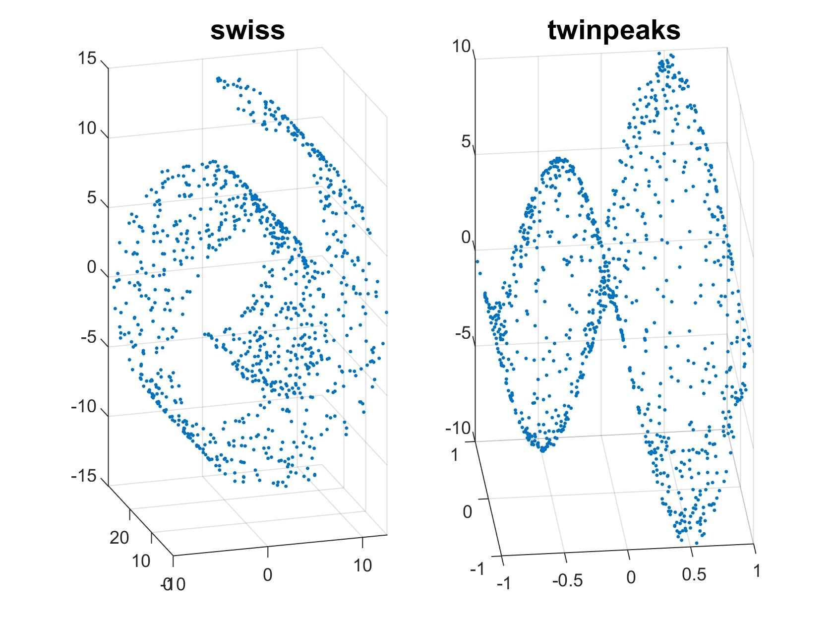
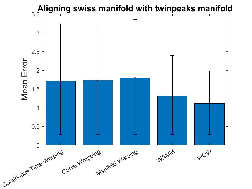
Figure 7: Top: A synthetic problem of aligning a swiss roll manifold with a twin peak manifold. The proposed WOW algorithm outperforms both previous methods, such as canonical time warping and manifold warping, as well as two alternative methods called curve wrapping and warping on mixed manifolds.

We illustrate the proposed methods with a simple synthetic example in Figure 7 of aligning two sampled manifolds, a regular swiss roll and a broken swiss roll. In the reprted experiments, alignment error is defined as follows. Let $p^{*}=[(1,1),\ldots,(n,n)]$ be the optimal alignment, and let $p=[p1,\ldots,p_{I}]$ be the alignment output by a particular algorithm. The error$(p,p^{*})$between $p$ and $p^{*}$ is computed by the normalized difference in area under the curve $x=y$ (corresponding to $p^{*}$) and the piece-wise linear curve obtained by connecting points in $p$. It has the property that $p\neq p^{*}\Rightarrow\mbox{error}(p,p^{*})\neq 0$.

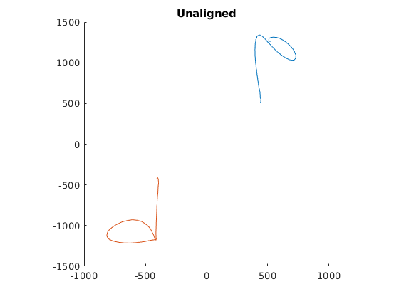
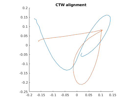
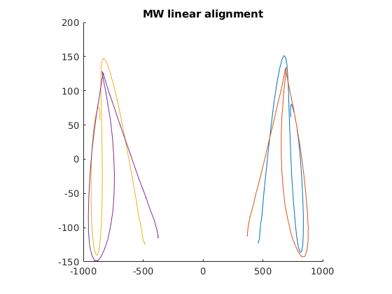
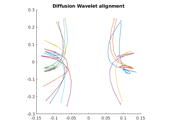
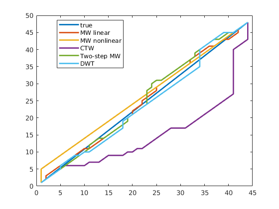
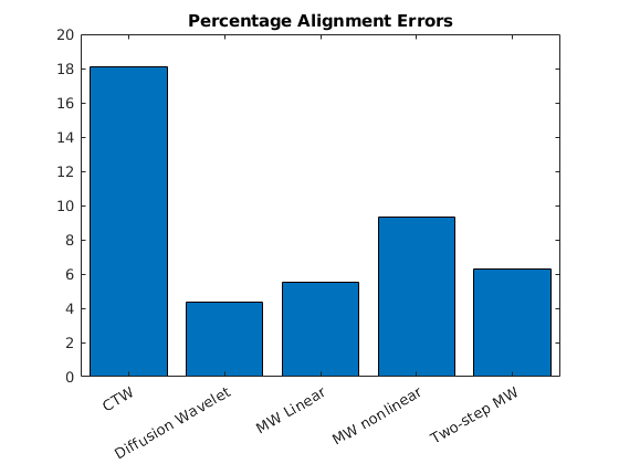
Figure 8: A synthetic problem of aligning rotated digits.

Figure 8 compares the performance of the proposed WOW algorithm against several other alignment algorithm on a synthetic rotated digit problem. The original problem is shown on the top left of the panel. The alignments produced by previous methods, such as canonical time-warping (Zhou and De la Torre, 2009) and manifold (linear, nonlinear, and two-step) warping (Vu et al., 2012), are compared against the newly proposed WOW algorithm that uses diffusion wavelets. The bottom left plot shows the alignments produced by each method against the ground truth ($45$ degree line). The bottom right panel computes the alignment error measured in terms of the area difference under each alignment curve vs. the ground truth.

7.2 Real World Datasets

Table 1 summarizes the various proposed novel algorithms and real-world domains used to compare them. The three real-world datasets used to test these algorithms are COIL, the Columbia Object Image Library (S. A. Nene, 1996), Human activity recognition (HAR), and the CMU Quality of Life dataset (De la Torre et al., 2008).

Method/Domain	COIL	UCI HAR	Quality of Life
WAMM	Figure 10	Figure 12	Figure 13
WOW	Figure 10	Figure 12	Figure 13
CW	Figure 10	Figure 12	Figure 13
Two-step CW	Figure 10	Figure 12	Figure 13
Manifold warping	Figure 10	Figure 12	Figure 13

Table 1: Proposed Algorithms and Experimental Domains

Table 2 lists the various hyper-parameters used in the above experiments.

	COIL	UCI HAR	CMU Quality of Life
$\mu$	0.5	0.5	0.5
$\tau$	1	1	1
$d$	2	2	2
$k$	10	10	10

Table 2: Hyperparameter settings for various datasets

7.2.1 COIL-100 data set

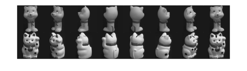
Figure 9: An example of a time-series alignment problem involving rotating objects.

The Columbia Object Image Library (COIL100) (S. A. Nene, 1996) corpus consists of different series of images taken of different objects on a rotating platform (Figure 9). Each series has $72$ images, each $128\times 128$ pixels. Figure 10 reports on experiments over 435 randomly chosen pairs of rotating objects from the COIL dataset, where WOW outperformed the other alignment methods. A paired T-test confirmed the hypothesis that WOW was indeed better to a significance of better than 99%.

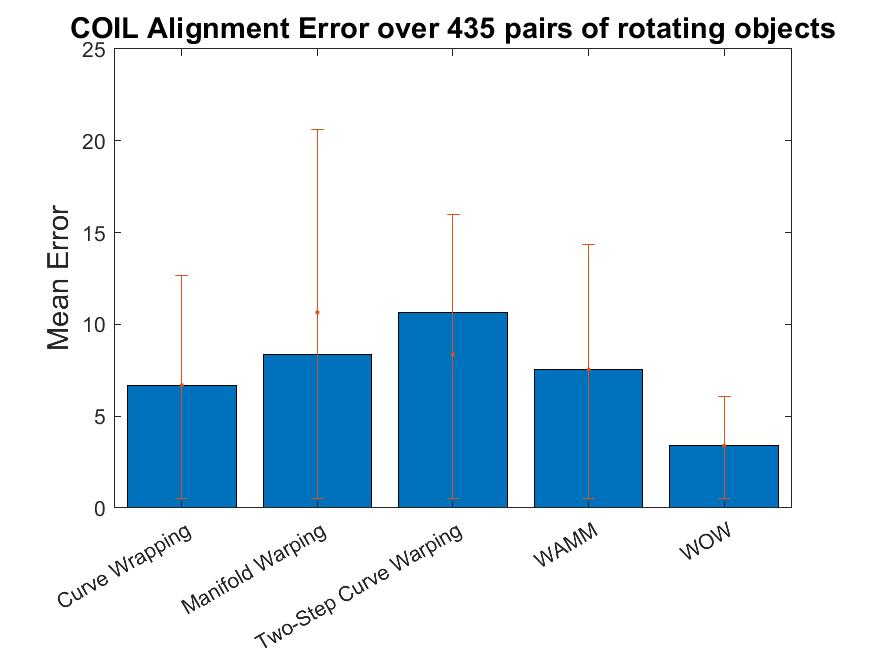
Figure 10: WOW outperforms other alignment algorithms in aligning rotating pairs objects in the COIL vision dataset.

7.2.2 Human Activity Recognition

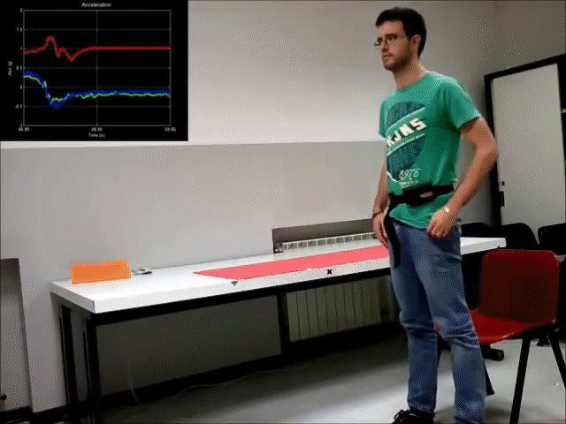
Figure 11: Human Activity Recognition using a Samsung smartphone.

The second real-world dataset involves recognition of human activities from recordings made on a Samsung smartphone (Reyes-Ortiz et al., 2014) (see Figure 11). . $30$ volunteers performed six activities (WALKING, WALKING UPSTAIRS, WALKING DOWNSTAIRS, SITTING, STANDING, LAYING) while wearing a smartphone (Samsung Galaxy S II) on the waist. Using its embedded accelerometer and gyroscope, 3-axial linear acceleration and 3-axial angular velocity measurements were captured at a constant rate of 50Hz. Figure 12 compares the WOW algorithm against the curve warping, as well as with two varieties of manifold warping. The results shown are averaged over $100$ trials, where each trial consisted of taking a subject and activity at random, and aligning the $3$-D accelerometer readings with the gyroscope readings. A paired T-test showed the differences between WOW and the other methods were statistically significant at the 95% or better level.

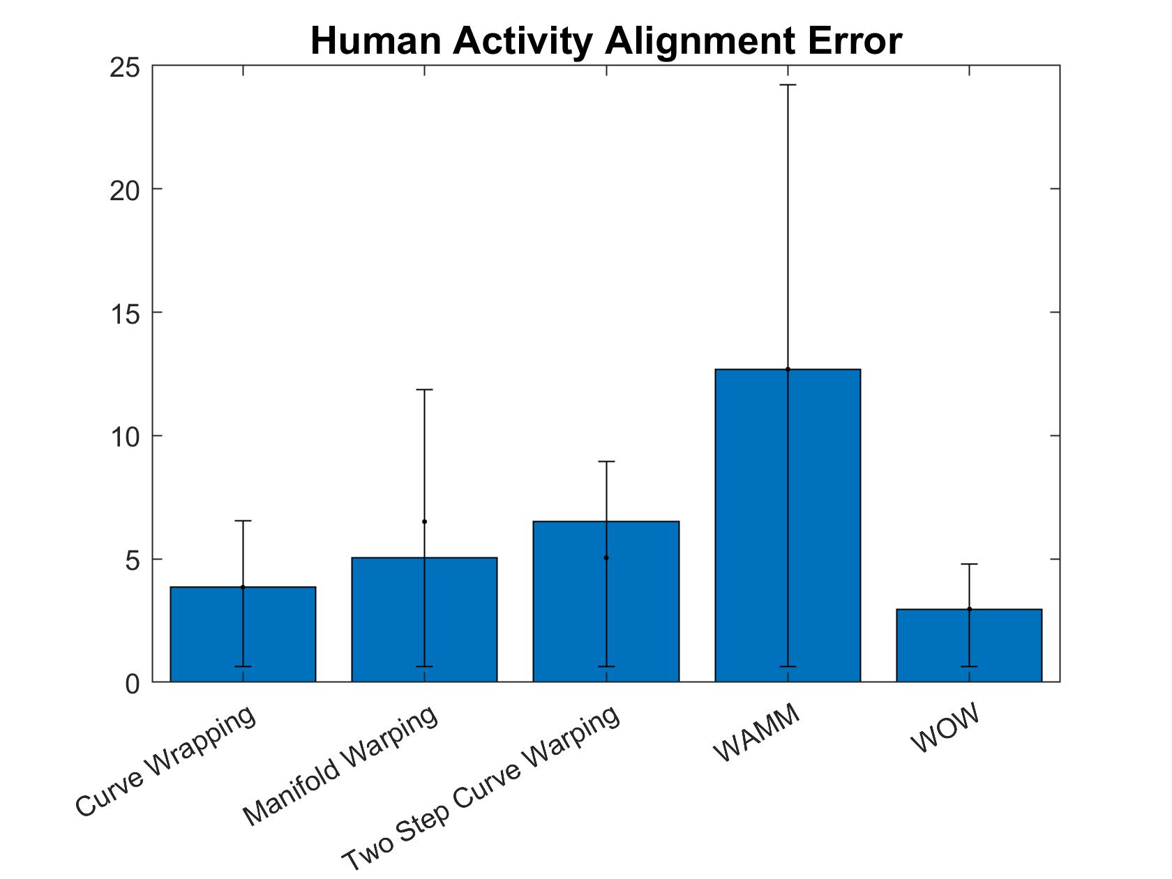
Figure 12: Experimental results on human activity recognition dataset showing mean alignment errors over 100 runs.

7.2.3 CMU Quality of Life Dataset

Our third real-word experiment uses the kitchen data set (De la Torre et al., 2008) from the CMU Quality of Life Grand Challenge, which records human subjects cooking a variety of dishes (see Figure 1). The original video frames are NTSC quality (680 x 480), which we subsampled to 60 x 80. We analyzed randomly chosen sequences of 100 frames at various points in two subjects’ activities, where the two subjects are both making brownies. As Figure 13 shows, WOW performs significantly better than the other methods, with a paired T-test showing significance better than 99% with p-values near 0.

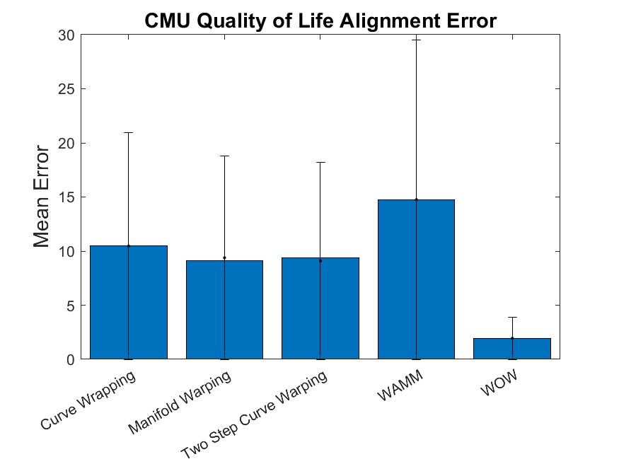
Figure 13: Mean alignment errors on CMU Quality of Life dataset of $25$ randomly chosen segments of $100$ video frames of two subjects making brownies.

8 Summary and Future Work

We introduced a novel multiscale time-series alignment framework called WOW, which combines dynamic time warping with diffusion wavelet analysis on graphs. WOW outperforms canonical time warping and manifold warping, two state of the art alignment methods, as well as other novel methods introduced in this paper, such as WAMM and curve wrapping. There are many directions for future work, including exploring faster variants of the proposed algorithms using distributed processors, combining our multiscale algorithms with nonlinear feature extraction methods using deep learning and related techniques, and doing more detailed experimental testing in additional domains.

References

• Anderson (2003) T.W. Anderson. An introduction to multivariate statistical analysis. Wiley series in probability and mathematical statistics. Probability and mathematical statistics. Wiley-Interscience, 2003. ISBN 9780471360919. URL http://books.google.com/books?id=Cmm9QgAACAAJ.
• Belkin and Niyogi (2001a) M. Belkin and P. Niyogi. Laplacian eigenmaps and spectral techniques for embedding and clustering. Advances in neural information processing systems, pages 585–591, 2001a.
• Belkin and Niyogi (2001b) M. Belkin and P. Niyogi. Laplacian eigenmaps and spectral techniques for embedding and clustering. Advances in neural information processing systems, 14:585–591, 2001b.
• Boucher et al. (2015a) Thomas Boucher, C. J. Carey, Sridhar Mahadevan, and Melinda Darby Dyar. Aligning mixed manifolds. In Blai Bonet and Sven Koenig, editors, Proceedings of the Twenty-Ninth AAAI Conference on Artificial Intelligence, January 25-30, 2015, Austin, Texas, USA, pages 2511–2517. AAAI Press, 2015a. URL http://www.aaai.org/ocs/index.php/AAAI/AAAI15/paper/view/9972.
• Boucher et al. (2015b) Thomas Boucher, C. J. Carey, Sridhar Mahadevan, and Melinda Darby Dyar. Aligning mixed manifolds. In Proceedings of the Twenty-Ninth AAAI Conference on Artificial Intelligence, January 25-30, 2015, Austin, Texas, USA., pages 2511–2517, 2015b. URL http://www.aaai.org/ocs/index.php/AAAI/AAAI15/paper/view/9972.
• Chung (1997) F. Chung. Spectral graph theory. Regional Conference Series in Mathematics 92, 1997.
• Coifman and Maggioni (2006) R. Coifman and M. Maggioni. Diffusion wavelets. Applied and Computational Harmonic Analysis, 21:53–94, 2006.
• De la Torre et al. (2008) F. De la Torre, J. Hodgins, A. Bargteil, X. Martin, J. Macey, A. Collado, and P. Beltran. Guide to the Carnegie Mellon University multimodal activity (CMU-MMAC) database, 2008.
• Favaro et al. (2011) P. Favaro, R. Vidal, and A. Ravichandran. A closed form solution to robust subspace estimation and clustering. IEEE Conference on Computer Vision and Pattern Recognition, pages 1801–1807, 2011.
• Ham et al. (2005) J. Ham, D. Lee, and L. Saul. Semisupervised alignment of manifolds. In Proceedings of the Annual Conference on Uncertainty in Artificial Intelligence, Z. Ghahramani and R. Cowell, Eds, volume 10, pages 120–127, 2005.
• He and Niyogi (2003) X. He and P. Niyogi. Locality preserving projections. In Proceedings of the Advances in Neural Information Processing Systems (NIPS), 2003.
• Junejo et al. (2008) Imran N. Junejo, Emilie Dexter, Ivan Laptev, and Patrick Pérez. Cross-view action recognition from temporal self-similarities. In David Forsyth, Philip Torr, and Andrew Zisserman, editors, Computer Vision – ECCV 2008, pages 293–306, Berlin, Heidelberg, 2008. Springer Berlin Heidelberg.
• Ma and Fu (2011) Y. Ma and Y. Fu. Manifold Learning Theory and Applications. CRC Press, 2011. ISBN 1439871094.
• Mallat (1998) S. Mallat. A wavelet tour in signal processing. Academic Press, 1998.
• Reyes-Ortiz et al. (2014) Jorge-Luis Reyes-Ortiz, Luca Oneto, Alessandro Ghio, Albert Samá, Davide Anguita, and Xavier Parra. Human activity recognition on smartphones with awareness of basic activities and postural transitions. In Stefan Wermter, Cornelius Weber, Włodzisław Duch, Timo Honkela, Petia Koprinkova-Hristova, Sven Magg, Günther Palm, and Alessandro E. P. Villa, editors, Artificial Neural Networks and Machine Learning – ICANN 2014, pages 177–184, Cham, 2014. Springer International Publishing.
• Rojas et al. (2020) Ignacio Rojas, Fernando Rojas, and Olga Valenzuela. Estimation of covid-19 dynamics in the different states of the united states using time-series clustering. medRxiv, 2020. doi:10.1101/2020.06.29.20142364. URL https://www.medrxiv.org/content/early/2020/06/29/2020.06.29.20142364.
• Roweis and Saul (2000) S.T. Roweis and L.K. Saul. Nonlinear dimensionality reduction by locally linear embedding. Science, 290(2323–232), 2000.
• S. A. Nene (1996) H. Murase S. A. Nene, S. K. Nayar. Columbia object image library (coil-100). Technical Report CUCS-006-96, February 1996.
• Sakoe and Chiba (1978) H. Sakoe and S. Chiba. Dynamic programming algorithm optimization for spoken word recognition. Acoustics, Speech and Signal Processing, IEEE Transactions on, 26(1):43–49, 1978.
• Vu et al. (2012) Hoa Trong Vu, Clifton Carey, and Sridhar Mahadevan. Manifold warping: Manifold alignment over time. In Proceedings of the Twenty-Sixth AAAI Conference on Artificial Intelligence, July 22-26, 2012, Toronto, Ontario, Canada., 2012.
• Wang and Mahadevan (2009) C. Wang and S. Mahadevan. A general framework for manifold alignment. In AAAI Fall Symposium on Manifold Learning and its Applications, 2009.
• Wang and Mahadevan (2013a) C. Wang and S. Mahadevan. Manifold alignment preserving global geometry. The 23rd International Joint conference on Artificial Intelligence, 2013a.
• Wang and Mahadevan (2013b) Chang Wang and Sridhar Mahadevan. Multiscale manifold learning. In Proceedings of the Twenty-Seventh AAAI Conference on Artificial Intelligence, July 14-18, 2013, Bellevue, Washington, USA., 2013b. URL http://www.aaai.org/ocs/index.php/AAAI/AAAI13/paper/view/6372.
• Zhou and De la Torre (2009) F. Zhou and F. De la Torre. Canonical time warping for alignment of human behavior. Advances in Neural Information Processing Systems (NIPS), pages 1–9, 2009.
• Zhou et al. (2008) F. Zhou, F. Torre, and J.K. Hodgins. Aligned cluster analysis for temporal segmentation of human motion. In Automatic Face & Gesture Recognition, 2008. FG’08. 8th IEEE International Conference on, pages 1–7. IEEE, 2008.