Theory of the Magnon Parametron

Abstract

The ‘magnon parametron’ is a ferromagnetic particle that is parametrically excited by microwaves in a cavity. Above a certain threshold of the microwave power, a bistable steady state emerges that forms an effective Ising spin. We calculate the dynamics of the magnon parametron as a function of microwave power, applied magnetic field and temperature for the interacting magnon system, taking into account thermal and quantum fluctuations. We predict three dynamical phases, viz. a stable Ising spin, telegraph noise of thermally activated switching, and an intermediate regime that at lower temperatures is quantum correlated with significant distillible magnon entanglement. These three regimes of operation are attractive for alternative computing schemes.

An Ising spin is a magnetic moment with a large uniaxial anisotropy that reduces the quantum degree of freedom of the Heisenberg spin on the Bloch sphere to just two, i.e. up and down. More generally, the term is used for any bistable system with a phase space of two distinct and stable configurations. For example, the magnetization of a fixed ferromagnetic needle that can point only into the two directions that minimizes the free energy is a (pseudo) Ising spin. An Ising spin with noise-activated transitions can operate as a probabilistic bit (p-bit), which in its steady state is a statistical mixture of the two levels. Ising spins are not useful as qubits because the large energy barrier prevents spin rotations on the Bloch sphere. Nevertheless, interactions with other degrees of freedom can induce quantum coherence of the Ising up and down spins and entanglement with other excitations. An ensemble of spins in these three regimes form a platform for unconventional computing algorithms. Switchable, but thermally stable, Ising spins are elements of “Ising machines” that can solve hard optimization problems [1, 2, 4, 3, 5], while network of p-bits can factorize large integers [6]. A relatively large ($\sim 2000$) and highly connected network of pseudo Ising spins with phase measurement and feedback was implemented by a train of optical parametric oscillators [2, 4, 3]. However, optical implementations have a large footprint and are not scalable. Quantum coherent networks are even more difficult to realize, but they can perform additional tasks such as quantum annealing, adiabatic evolution, or gated quantum operations [8, 7, 10, 9, 12, 11].

Parametric pumping is a standard method to excite large oscillations in a harmonic oscillator by a phase matched drive at twice the resonance frequency $\omega_{0}$. When a harmonic oscillator with Hamiltonian $\hbar\omega_{0}a^{{\dagger}}a$, where $a^{{\dagger}}\left(a\right)$ creates (annihilates) a boson, has non-linear interaction with photons, it can be driven into an instability by the parametric term $Pe^{2i\omega_{0}t}a^{{\dagger}}a^{{\dagger}}+\mathrm{H.c.}$, when the classical amplitude $P$ exceeds a certain threshold. In the steady state, the mean field $\langle a\rangle$ spontaneously acquires either one of the energetically equivalent phases of $\phi_{p}/2+0$ or $\phi_{p}/2+\pi$, where $\phi_{p}=\mathrm{\arg}Pe^{2i\omega_{0}t}$ and $2\operatorname{mod}\mathrm{\arg}\left[\langle a\rangle,2\pi\right]=\operatorname{mod}\left[\phi_{p},2\pi\right]$, which can be mapped on the two states of a pseudo Ising spin. Such oscillators can be realized by optical [2, 4, 3], electromechanical [13], or magnetic [14] systems. Makiuchi et al. [14] demonstrated a “magnon parametron” on a disk of the magnetic insulator yttrium iron garnet (YIG) that also showed the stochastic behavior expected for a p-bit.

A Hilbert space of a quantum system is ‘discrete’ when its dimension is countable, e.g., two for a spin-$1/2$ system. It is called ‘continuous’ when uncountably infinite, e.g. when spanned by position and momentum variables of a harmonic oscillator. The lowest number states of the Kittel magnons, i.e. the quanta of the uniform precession of the magnetic order [16, 15, 17] enable ‘discrete variable’ quantum information processing [18, 19]. However, since their anharmonicity is small, an auxiliary superconducting qubit is required to manipulate the quantum states of the lowest magnon levels. On the other hand, strongly driven magnons alone offer ‘continuous variable’ quantum information such as entanglement, photon squeezing, and antibunching [20, 21, 22]. Magnons are also set apart from e.g. phonons [23] by their highly tunable, anisotropic and non-monotonic dispersions. Parametric excitation of magnets generates large magnon numbers that live long enough to form Bose-Einstein condensates [24, 25, 26, 27]. We are especially interested in the efficient and distillable entanglement of magnons [21] in the parametrically excited regime.

In this Letter, we address the theory of the ‘magnon parametron’ [14], i.e. a thin film magnetic disc that is parametrically excited in a microwave cavity. We show that it can operate as an Ising spin that is tuned between deterministic, stochastic, and quantum regimes, which should be considered seriously as a platform for alternative computing technologies. The Suhl instability [28, 21], i.e. the decay of the uniform (Kittel) magnon into a pair of magnons with opposite momenta $\pm{k}\neq 0$, can be reached by driving magnon parametrically by cavity-mode microwaves with a small amplitude when quality factors are high. At a classical fixed point of the magnetization dynamics and at cryogenic temperatures we predict a distillable quantum entanglement [21]. The limit-cycle dynamics at slightly higher photon amplitudes enables the observed stochastic switching between the Ising spin states [14] only when the ‘wing’ magnons are involved.

Model - Figure 1(a) sketches a thin ferromagnetic disk of thickness $d$ and radius $r$, uniformly magnetized along the in-plane magnetic field $\vec{H}_{ext}\|\hat{z}$. The microwave magnetic field $\vec{h}_{mw}\|\hat{z}$ of a cavity or a coplanar waveguide mode with frequency $\omega_{p}$ is polarized along the magnetization. Figure 1(b) shows the magnon frequency dispersions $\omega_{\vec{k}}$ of a typical YIG disk of $d=50\,$nm, corresponding to $\theta_{\vec{k}}=0$ ($\vec{k}\|\hat{z}$) and $\theta_{\vec{k}}=\pi/2$ ($\vec{k}\perp\hat{z}$) for in-plane wave vectors and constant magnetization along $\hat{x}$, i.e. the lowest magnon subband [30, 31, 29]. $\omega_{0}$ is the frequency of the Kittel mode. A node along $\hat{x}$ blue-shifts the entire dispersion $\sim 4\gamma D/d^{2}\sim 0.2\,$GHz relative to the bulk value of Fig. 1(b), where $\gamma=26\,\text{GHz}$/T is the gyromagnetic ratio and $D=2\times 10^{-17}\,\text{T}\text{m}^{2}$ is the exchange stiffness [32]. We restrict our study to the lowest subband since for the chosen dimensions $\omega_{\vec{k}_{\mathrm{dip}}}+4\gamma D/d^{2}>\omega_{0}$, where $\omega_{\vec{k}_{{}_{\mathrm{dip}}}}$ is the frequency minimum caused by the magnetodipolar interaction. The two valleys in the magnon dispersion are essential for the Suhl instability and exist when $r\gtrapprox 0.5\,\mathrm{\mu}$m.

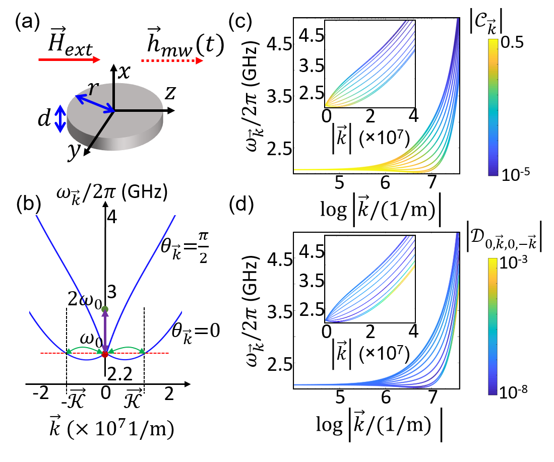
Figure 1: Model. (a) A magnetic disk of thickness $d$ and radius $r$ under static and microwave magnetic fields. (b) The dispersion envelope of magnons with constant magnetization along $x$ for $d=50\,$nm and $r=100\,\mathrm{\mu}$m. The green arrows indicate 4-magnon scattering processes involving the Kittel mode. The purple line indicates parametric pumping of the Kittel mode. (c) The parametric excitation coefficient amplitude $\mathcal{C}_{\vec{k}}$ of the magnon pairs overlaid on the dispersion for several values of $\theta_{\vec{k}}$ from $0$ to $\pi/2$, only for the modes nodeless along the thickness. (d) Similar to (c) but for the 4-magnon scattering coefficient $\mathcal{D}_{0,\vec{k},0,-\vec{k}}$. The insets of (c) and (d) plot the data of the main panels on a linear momentum scale..

Figure 1(b) sketches the Kittel mode and a degenerate pair of magnons with wave vector $\pm\mathcal{K}$ as well as the four-magnon scattering process relevant to a Suhl instability. $\vec{h}_{mw}(t)$ with frequency $\omega_{p}=2\omega_{0}$ parametrically interacts with the Kittel mode and the degenerate magnon pairs. Our Hamiltonian contains the leading terms of the Holstein-Primakoff expansion of the Heisenberg model, including all 4-magnon interactions [33, 21, 34]

$$H =H_{m,L}+H_{m,NL}+H_{mp}+{H_{p}},$$

$$H_{m,L} =\sum_{\vec{k}}\omega_{\vec{k}}c_{\vec{k}}^{{\dagger}}c_{\vec{k}}$$

$$H_{m,NL} =\sum_{\vec{k}}\left\{\mathcal{D}_{\vec{k},\vec{k},\vec{k},\vec{k}}c_{\vec{k}}^{{\dagger}}c_{\vec{k}}c_{\vec{k}}^{{\dagger}}c_{\vec{k}}+\right.$$

$$\sum_{\vec{k}^{\prime\prime}}\left[\left(1-\delta_{\vec{k},\vec{k}^{\prime\prime}}\right)\mathcal{D}_{\vec{k},\vec{k},\vec{k}^{\prime\prime},\vec{k}^{\prime\prime}}c_{\vec{k}}^{{\dagger}}c_{\vec{k}}c_{\vec{k}^{\prime\prime}}^{{\dagger}}c_{\vec{k}^{\prime\prime}}+\right.$$

$$\left.\left.\left(1-\delta_{|\vec{k}|,|\vec{k}^{\prime\prime}|}\right)\frac{1}{2}\mathcal{D}_{\vec{k},\vec{k}^{\prime\prime},-\vec{k},-\vec{k}^{\prime\prime}}c_{\vec{k}}^{{\dagger}}c_{-\vec{k}}^{{\dagger}}c_{\vec{k}^{\prime\prime}}c_{-\vec{k}^{\prime\prime}}\right]\right\},$$

$$H_{mp} =\sum_{\vec{k}}\frac{1}{2}\left(1+\delta_{\vec{k},0}\right)\left(\mathcal{G}_{\vec{k}}bc_{-\vec{k}}^{{\dagger}}c_{\vec{k}}^{{\dagger}}+H.c.\right),$$

$$H_{p} =\omega_{p}b^{{\dagger}}b+E\left(b^{{\dagger}}+b\right),$$ (1)

where $\mathcal{G}_{\vec{k}}=\gamma\mathcal{C}_{\vec{k}}\sqrt{\hbar\mu_{0}\omega_{p}/2V_{p}}$, $b$ is the photon annihilation operator, $V_{p}$ is the cavity mode volume, $m_{z}=1-\sum_{\vec{k}}\left[c_{\vec{k}}^{{\dagger}}c_{\vec{k}}+\left(\mathcal{C}_{\vec{k}}c_{-\vec{k}}^{{\dagger}}c_{\vec{k}}^{{\dagger}}+\mathrm{H.c.}\right)\right]/S$ is the $\hat{z}$ component of the magnetization unit vector, the total spin $S=M_{s}V_{m}/2\pi\gamma\hbar$, $V_{m}$ is the volume of the sample, $M_{s}$ is the saturation magnetization. The coefficients $\mathcal{C}$ and $\mathcal{D}$ are complicated but well known [34, 33].

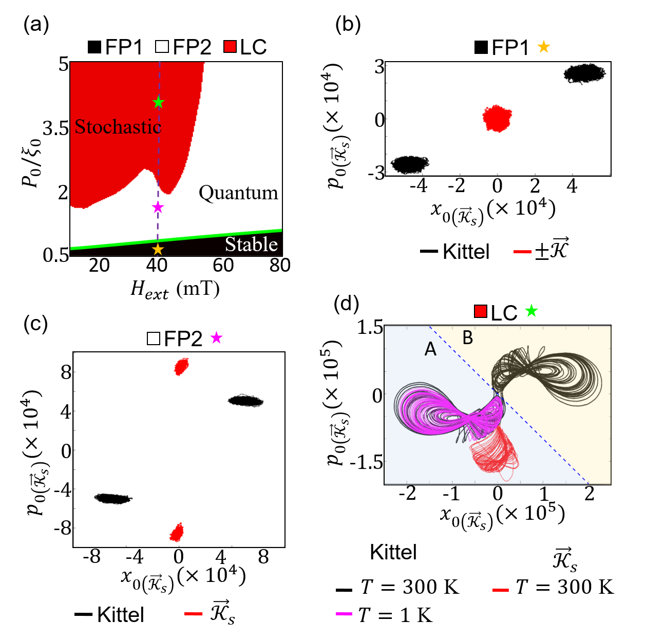
Figure 2: Calculated steady-state dynamics of a magnet in a microwave cavity. (a) The dependence of steady-state class on the Kittel mode amplitude $P_{0}$ driven by the mircrowaves and the dc magnetic field $H_{\mathrm{ext}}$, labeled as ‘Stable’, ‘Quantum’, and ‘Stochastic’. (b)-(d) Examples for the three distinct classes, corresponding to the stars of the same color in in (a), $P_{0}/\xi_{0}=0.7,\,1.7,\,3.8$, respectively, while $H_{ext}=40\,$mT. (b) FP1: Fixed point, the Kittel mode parametrically driven beyond threshold, while the $\vec{\mathcal{K}}_{s}$ pair at vacuum. FP2: Fixed point, the Kittel mode and $\vec{\mathcal{K}}_{s}$ standing wave parametrically and Suhl instability driven, respetively. In (b) and (c), $T=3\times 10^{5}\,$K for clarity. (d) LC: Limit cycle to chaos. A case with large transition rate from one attractor region of the Kittel mode to the other, at $T=300\,$K, and no transition for $T=1\,$K also shown. The two attractor regions A and B indicated. In (b) and (c), green trajectories are for $\mathcal{K}$ standing wave.

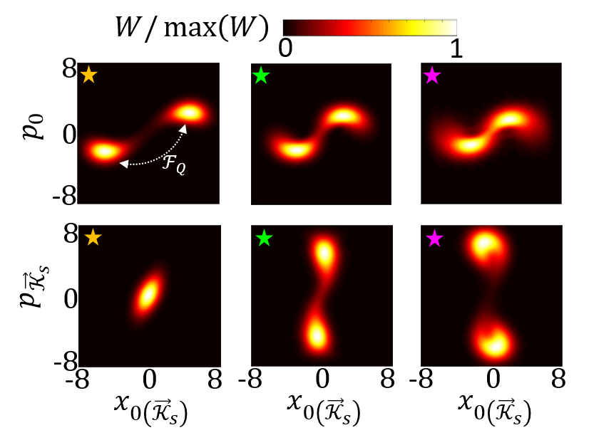
Figure 3: Quantum steady states. The top (bottom) panels are the Wigner function of the Kittel mode ($\mathcal{K}$ standing wave) normalized by the maximum value. The left, middle, and right panels correspond to the star of the same color as in Fig. 2(a), as well as Figs. 2(b)-(d), i.e., in the FP1 (Ising), ‘Quantum’ (FP2), and ‘Stochastic’ (LC) regions, respectively. The scaling of four-magnon scattering coefficients $\mathcal{Q}=5\times 10^{8},\,2\times 10^{9},\,4\times 10^{9}$, from left to right panels, respectively.

Here we pump the precession cone angle of spin waves by the microwave magnetic field along the magnetization. The photon drive $E$ with $\omega_{p}\sim 2\omega_{0}$ leads to a coherent photon field $\langle b\rangle=\beta$ such that $\mathcal{G}_{\vec{k}}\beta c_{-\vec{k}}^{{\dagger}}c_{\vec{k}}^{{\dagger}}+\mathrm{H.c}.$ can parametrically excite the Kittel mode and magnon pairs with $\omega_{\vec{k}}\sim\omega_{p}/2$. When increasing $E,$ the mode with the largest $\mathcal{G}_{\vec{k}}\propto\mathcal{C}_{\vec{k}}$ becomes instable at a critical value $\mathcal{G}_{\vec{k}}\beta=\xi_{\vec{k}}/2$, where $\xi_{\vec{k}}\approx\alpha_{G}\omega_{\vec{k}}$ is the magnon dissipation rate in terms of $\alpha_{G}$, the Gilbert damping constant. $|\mathcal{C}_{\vec{k}}|$ in Figure 1(c) is maximal for small wave vectors, which implies that the Kittel mode becomes instable first. The “drift” matrix $\mathcal{O}=\left[i\omega_{0}-\xi_{0}/2,i\mathcal{G}_{0}\beta;-i\mathcal{G}_{0}\beta,-i\omega_{0}-\xi_{0}/2\right]$ of the linear equation of motion $\left[\dot{c}_{0},\dot{c}_{0}^{{\dagger}}\right]^{T}=\mathcal{O}\left[{c}_{0},{c}_{0}^{{\dagger}}\right]^{T}$ then acquires an eigenvalue with positive real part. The so-called self-Kerr coefficient $\mathcal{D}_{0,0,0,0}$ governs steady state Kittel magnon amplitude just above the threshold. Here we use rather large damping parameter $\xi_{0}=5\,$MHz corresponding to $\alpha_{G}\sim 2\times 10^{-3}$ for computational convenience.

The parametrically driven Kittel mode excites other magnons via the four-magnon scattering term $c_{0}^{{\dagger}}c_{0}^{{\dagger}}c_{\vec{k}}c_{-\vec{k}}+\mathrm{H.c.}$, where Fig. 1(d) plots the corresponding coefficients $\left|\mathcal{D}_{0,\vec{k},0,-\vec{k}}\right|$. This is another threshold process introduced first by Suhl [28]. Ignoring the terms $c_{0}^{{\dagger}}c_{0}c_{\pm\vec{k}}^{{\dagger}}c_{\pm\vec{k}}$ for the moment, the instability is reached when the amplitude of the Kittel mode mean field $\left|\alpha_{0}\right|=\langle c_{0}\rangle=\left(\sqrt{\xi_{\vec{k}}^{2}/4+\Delta_{\vec{k}}^{2}}/|\mathcal{D}_{0,\vec{k},0,-\vec{k}}|\right)^{1/2}$. This happens first for the degenerate modes with largest $\left|\mathcal{D}_{0,\vec{k},0,-\vec{k}}\right|$, i.e. for $\theta_{\vec{k}}=0$ and large $\left|\vec{k}\right|$ and thereby limits the Hilbert space to three modes, the parametrically pumped Kittel mode and a pair of magnons with large wave vector $\pm\mathcal{\vec{K}}$. In the rotating frame of $\mathcal{\omega}_{p}/2,$ the Hamiltonian (1) reduces to $H^{\prime}=H_{m,L}^{\prime}+H_{m,NL}^{\prime}+P_{0}\left(c_{0}^{{\dagger}}c_{0}^{{\dagger}}+\mathrm{H.c}.\right)$, where $H_{m,L}=\sum_{\vec{k}\in{\{0,\pm\mathcal{K}\}}}\Delta\omega_{\vec{k}}c_{\vec{k}}^{{\dagger}}c_{\vec{k}}$, $\Delta\omega_{\vec{k}}=\omega_{\vec{k}}-\omega_{p}/2$, $H_{m,NL}^{\prime}=\left.H_{m,NL}\right|_{\vec{k}\in\{0,\pm\mathcal{K}\}}$. The critical parametric excitation amplitude $P_{0}=\xi_{0}/2$ corresponds to a photon amplitude $E\approx P_{0}\xi_{p}/2\mathcal{G}_{0}$ and power $\mathcal{P}=E^{2}\hbar\omega_{p}/\xi_{p}=P_{0}^{2}\xi_{p}\hbar\omega_{p}/4\mathcal{G}_{\vec{k}}^{2}$. Assuming $\xi_{p}=10\,$kHz (photon quality factor $\sim 10^{5}$), and $\mathcal{G}_{\vec{k}}/\mathcal{C}_{\vec{k}}=10$ which corresponds to a photon mode volume $V_{p}\sim 10^{-2}\,\mathrm{mm}^{3}$, for $P_{0}=\xi_{0}/2$, $\mathcal{P}\approx 2\,\mathrm{\mu W}$ and for $P_{0}=5\xi_{0}$ (maximum value used in our calculations), $\mathcal{P}\approx 0.2\,$mW.

The (Lindblad) equation of motion of the density matrix $\rho$ with elements $\rho_{i,j}=\left|i\right\rangle\left\langle j\right|$, where $|i(j)\rangle$ is a many-body number (Fock) state of the magnon system, reads

$$\dot{\rho}=-i\left[H^{\prime},\rho\right]+L_{d},$$ (2)

where

$$L_{d} =\sum_{\vec{k}\in\{0,\pm\mathcal{K}\}}\xi_{\vec{k}}\left[n_{th}(\omega_{\vec{k}})\left(c_{\vec{k}}\rho c_{\vec{k}}^{{\dagger}}+c_{\vec{k}}^{{\dagger}}\rho c_{\vec{k}}-\rho c_{\vec{k}}c_{\vec{k}}^{{\dagger}}-\right.\right.$$

$$\left.\left.c_{\vec{k}}^{{\dagger}}c_{\vec{k}}\rho\right)+\frac{1}{2}\left(2c_{\vec{k}}\rho c_{\vec{k}}^{{\dagger}}-c_{\vec{k}}^{{\dagger}}c_{\vec{k}}\rho-\rho c_{\vec{k}}^{{\dagger}}c_{\vec{k}}\right)\right],$$ (3)

is the dissipation operator of the magnons in contact with a thermal bath. Here $n_{th}(\omega_{\vec{k}})=\left(e^{\hbar\omega_{\vec{k}}/k_{B}T}-1\right)^{-1}$, $k_{B}$ is the Boltzmann constant, and $T$ is the bath temperature. We disregard nonlinear radiative damping terms since $|\gamma\mathcal{C}_{\vec{k}}\sqrt{\hbar\mu_{0}\omega_{p}/2V_{p}}|^{2}/\xi_{p}\xi_{0}\ll 1$ [35]. Without drive, $\rho$ describes a magnon gas at thermal equilibrium with the bath.

Next, we show our results for the driven steady state, quantify stochasticity, and discuss quantum entanglement in our magnetic dot.

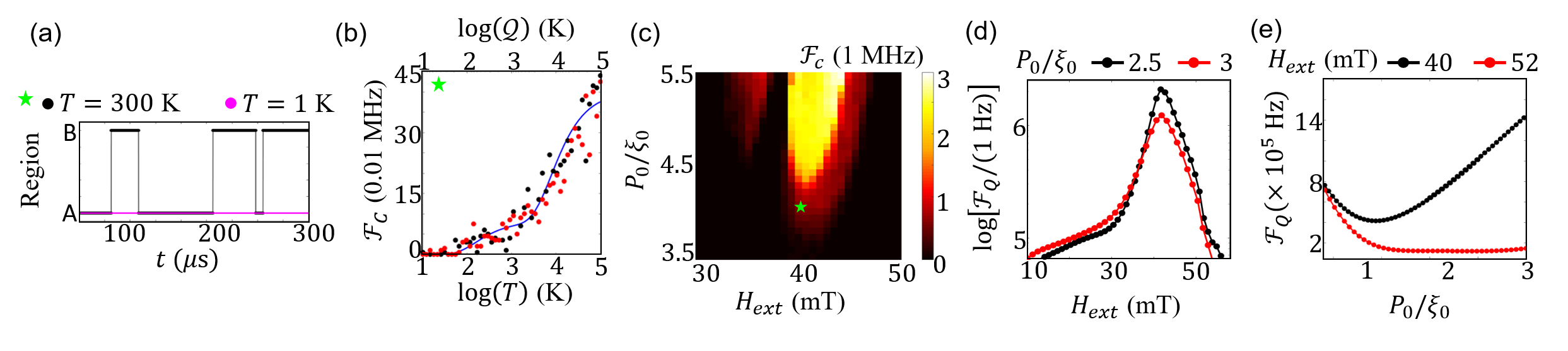
Figure 4: Stochasticity. (a)-(c) From semi-classical, (d)-(f) from quantum calculations. (a) The region of the Kittel mode state shown in Fig. 2(d) for $T=1\,$K and $T=300\,$K. (b) The dependence of transition frequency $\mathcal{F}_{C}$ on $T$ (black dots) and $\mathcal{Q}$ (red dots), for $\ H_{\mathrm{ext}}=40\,\text{mT},P_{0}/\xi_{0}=3.85$, as in (a) and Fig. 2(d). (c) $\mathcal{F}_{C}$ as a function of $H_{\mathrm{ext}}$ and $P_{0}/\xi_{0}$, at $T=3\times 10^{5}\,$K. The green star is the same $(P_{0},H_{\mathrm{ext}})$ point as in the phase diagram plotted in Figs. 2(a) and (d). (d) The dependence of tunneling frequency $\mathcal{F_{Q}}$ on $H_{ext}$ for two values of $P_{0}/\xi_{0}=2.5,\,3$. (e) The dependence of $\mathcal{F}_{Q}$ on $P_{0}/\xi_{0}$ for $H_{ext}=40,\,52\,$mT, respectively. The scaling coefficient $\mathcal{Q}=5\times 10^{9}$ in (d)-(e), and $T=0\,$K.

Steady state classes - We classify the steady state dynamics in terms of a “phase diagram” of our three-mode system by the solutions of the Langevin equation of motion. Disregarding the third and fourth order derivatives of the Wigner distribution functions as described in the supplementary material (SM), Sec. I [38, 36, 37] for small nonlinearities, simplifies the equation of motion to $\dot{v}=-i[H,v]+\Gamma$, where $v=[x_{0},p_{0},x_{\mathcal{K}},p_{\mathcal{K}},x_{-\mathcal{K}},p_{-\mathcal{K}}]$, $x_{0(\pm\vec{\mathcal{K}})}=(c_{0(\pm\vec{\mathcal{K}})}+c_{0(\pm\vec{\mathcal{K}})}^{{\dagger}})/2$, $p_{0(\pm\vec{\mathcal{K}})}=-i(c_{0(\pm\vec{\mathcal{K}})}-c_{0(\pm\vec{\mathcal{K}})}^{{\dagger}})/2$, and $\Gamma$ represents fluctuating fields with Gaussian quantum statistics. We solve this 6-dimensional Langevin differential equation in real time starting from appropriate initial conditions until the steady state is reached.

The microwaves parametrically excite the Kittel mode with detuning $\Delta\omega_{0}=0$, and an amplitude $P_{0}$. The other control parameter is the applied static magnetic field $H_{ext}$. The smallest positive solution for $x=|\alpha_{0}|^{2}$ governs $\theta_{\vec{\mathcal{K}}}$ and $|\vec{\mathcal{K}}|$ of the magnon pair that reaches the Suhl instability first

$$\left(\mathcal{D}_{0,\vec{\mathcal{K}},0,-\vec{\mathcal{K}}}^{2}-\mathcal{D}_{0,0,\vec{\mathcal{K}},\vec{\mathcal{K}}}^{2}\right)x^{2}-2\Delta_{\vec{\mathcal{K}}}\mathcal{D}_{0,0,\vec{\mathcal{K}},\vec{\mathcal{K}}}x$$

$$-\xi_{\vec{\mathcal{K}}}^{2}/4-\Delta_{\vec{\mathcal{K}}}^{2}=0.$$ (4)

Below the Suhl but above the parametric instability threshold $|\alpha_{0}|^{2}=\sqrt{P_{0}^{2}-\xi_{0}^{2}/4}/2|\mathcal{D}_{0,0,0,0}|$.

With notation $c_{\pm\mathcal{K}}=|c_{\pm\mathcal{K}}|e^{i\phi_{\pm\vec{\mathcal{K}}}},$ the four magnon scatterings fix the sum of the phases $\phi_{+}=\phi_{\vec{\mathcal{K}}}+\phi_{-\vec{\mathcal{K}}}$, but the difference $\phi_{-}=\phi_{\vec{\mathcal{K}}}-\phi_{-\vec{\mathcal{K}}}$ is not uniquely determined [40]. The magnetic disc has a large but finite radius, that strictly speaking splits the continuum of state by $\triangle\nu\sim 2n\gamma D/r^{2}\sim 10^{4}\text{Hz}$, where $n=\lfloor 2r\mathcal{K}\rfloor\sim 4000$. Since $\triangle\nu\ll\xi_{0},$ the spectrum is still quasi-continuous, but the Kittel mode decays not into two propagating, but a single standing wave mode. This can be formalized by combining the $\pm\vec{\mathcal{K}}$ pair of propagating waves as $c_{\pm\vec{\mathcal{K}}}=c_{\vec{\mathcal{K}}_{s}}e^{\mp iq/2}$ [39, 40], where the phase $q=\phi_{-}$ is a free phase that governs the position of the standing wave nodes and $\vec{\mathcal{K}}_{s}$ is a standing wave index. This reduction of a three-partite into a two-partite problem simplifies the quantum regime calculations.

Figure 2(a) shows the steady state classes as a function of $H_{\mathrm{ext}}$ and $P_{0}$, obtained numerically for $T=0\,$K. The green line in Fig. 2(a) is an analytic solution of Eq. (4) using the four-magnon scattering parameters of the unstable mode for each $H_{\mathrm{ext}}$. The phase-space dynamics of each class are illustrated by Figs. 2(b)-(d) for a fixed magnetic field. Figures 2(b) and (c) show trajectories in the time interval $t=50-80\,\mathrm{\mu}$s, starting from 100 random initial values of $\phi_{0(\vec{\mathcal{K}}_{s})}$ in $c_{0(\vec{\mathcal{K}}_{s})}=e^{i\phi_{0(\vec{\mathcal{K}}_{s})}}$ at $t=0\$and a high temperature $T=3\times 10^{5}\,$K to emphasize the dynamic stability. The trajectories are depicted in $(x_{0(\vec{\mathcal{K}}_{s})},p_{0(\vec{\mathcal{K}}_{s})})$ phase space. We observe two distinct classes that are characterized by Kittel mode fixed-points FP1 and FP2. For a given $H_{\mathrm{ext}}$ and small $P_{0}>\xi_{0}/2$ (FP1) the Kittel mode has two equivalent stable fixed points (Ising spin up and down), while $\vec{\mathcal{K}}_{s}$ standing wave mode only fluctuates around the origin [see Fig. 2(b)]. When $P_{0}$ satisfies Eq. (4), the Suhl instability drives the $\pm\mathcal{K}$ pair, leading to the FP2 steady state in which the Kittel fixed points persist, and $\vec{\mathcal{K}}_{s}$ settles at a fixed point away from the origin with a phase spontaneously chosen out of two mirror symmetric values [see Fig. 2(c)]. We note that even though FP2 is labeled “quantum”, at the chosen high temperatures all quantum correlations are of course washed out (see below). A third distinct class without a stable fixed point is the limit cycle (LC) illustrated in Figure 2(d) for realistic temperatures. For certain $H_{\mathrm{ext}}$ and not too large $P_{0}$, the Kittel mode follows large amplitude trajectories in mirror symmetric regions of the phase space (see also SM Sec. IV [38]). With increasing $P_{0}$ the paths cross the boundaries between attractor regions A and B. The thermal activation becomes clear from Figure 2(d) that compares switching at high $T=300\,$K (black curve), and low $T=1\,$K (purple curve), where we show single representative trajectories in the interval $t=20-320\,\mathrm{\mu}$s. We elaborate this stochasticity below. In SM Sec. IV [38], we discuss the dependence of the limit cycle trajectories on $P_{0}$ (see Fig. S4 [38]), and analytically explain the origin of FP2 to LC transition, and its dependence on $H_{ext}$ (see Fig. S5 [38]).

The Lindblad master equation can be solved in principle numerically exact in number (Fock) space. With our computational facilities the Hilbert space has to be limited to $\sim 1000$, which is much too small to treat the essential Hilbert space of a large magnet. We can reduce the Hilbert space to a manageable size by introducing a scaling factor of the four-magnon scattering coefficients $\mathcal{D}\rightarrow\mathcal{Q}\mathcal{D}$ with $\mathcal{Q}\gg 1$. The increased interaction preserves the topology in phase space, but reduces the magnon amplitudes and thereby the relevant size of the Fock space. As explained above, selecting the standing wave $\mathcal{\vec{K}}_{s}$, reduces the 3-mode to a 2-mode problem. We calculate up to 20 smallest amplitude eigenvalues $\mathcal{E}\geq 0$ of the r.h.s. of Eq. (2), in which the $\mathcal{E}=0$ corresponds to the ground state density matrix $\rho_{ss}$. We visualize the steady states by the Wigner distribution function $W(x_{0(\vec{\mathcal{K}}_{s})},p_{0(\mathcal{K}_{s})})=\int\langle x_{0(\vec{\mathcal{K}}_{s})}-y/2|\rho_{ss,0(\vec{\mathcal{K}}_{s})}|x_{0(\vec{\mathcal{K}}_{s})}+y/2\rangle e^{ip_{0(\vec{\mathcal{K}}_{s})}y}dy$ of the Kittel ($\vec{\mathcal{K}}_{s}$) mode, where $|x_{0(\vec{\mathcal{K}}_{s})}\pm y/2\rangle$ is the position eigenstate of the Kittel ($\vec{\mathcal{K}}_{s}$) mode, and $\rho_{ss,0(\vec{\mathcal{K}}_{s})}$ is the density matrix after tracing out the $\vec{\mathcal{K}}_{s}$ (Kittel) mode. The top (bottom) panels of Fig. 3 show $W(x_{0(\vec{\mathcal{K}}_{s})},p_{0(\vec{\mathcal{K}}_{s})})$ for $H_{ext}=40\,$mT in each of the ‘Stable’, ‘Quantum’, and ‘Stochastic’ phases, as indicated by stars of the same color in Fig. 2(a). The left and middle panels can be compared with the classical phase space of FP1 and FP2 in Figs. 2(b) and (c), respectively. The right panel of Fig. 3 should be compared with the limit cycle region in the classical phase space, e.g., in Fig. 2(c). In the panels of Fig. 3, we used different scale factors $\mathcal{Q}$ such that the distance between the extrema of $W$ is roughly the same.

The steady state classes FP1, FP2, and LC [see Fig. 2(a)] are potential resources for information technologies. For a fixed input power of $P_{0}$ the stable Ising spin can be used as a non-volatile digital memory, while a network can operate as an Ising machine. We can assess the potential of the device as p-bit or for quantum information by quantitative measures of the stochasticity and entanglement derived from our semi-classical (quantum) calculations indicated in the following by a subscript or superscript ‘C’ (‘Q’). In ‘C’, we solve the quantum Langevin equation of motion for Gaussian distribution functions. In the quantum calculations, on the other hand, we solve the master equation (2) in the number (Fock) space, and the solutions are numerically exact, but due to computational limitations we can solve only down-scaled systems, as explained above.

Stochasticity - The lower bound for the transition time $\tau$ between the two stable fixed points below the Suhl instability threshold (derived in SM Sec. IIB [38]) is

$$\mathrm{\ln}\tau \gtrapprox\ln\left[\pi\left(1+2n_{\mathrm{th}}\right)\sqrt{(1+2\mathcal{R})/2\mathcal{R}^{2}}/2\xi_{0}\right]+$$

$$\left[\left(2\mathcal{R}+1\right)\ln\left(2\mathcal{R}+1\right)-2\mathcal{R}\right]|K_{0}|\left(1+2n_{\mathrm{th}}\right)/2,$$ (5)

where $\mathcal{R}=\sqrt{\mu^{2}-1}/2+1-|K_{0}|\left(1+2n_{\mathrm{th}}\right)-1$, $\mu=2P_{0}/\xi_{0}$, $K_{0}=2\mathcal{D}_{0,0,0,0}/\xi_{0}$. Above the parametric instability threshold but below the Suhl instability $\left(\mu=1.1\right)$ for typical values of $|\mathcal{D}_{0,0,0,0}|=1.5\times 10^{-4}\,$Hz (see Fig. S5(a) [38]), $\omega_{0}/2\pi=2.5\,$GHz [see Fig. 1(b)], and $T=300\,$K, this number becomes astronomically large, $\tau\gg\exp(1.4\times 10^{4})\,$s. However, by driving the system into a limit cycle of the Kittel plus $\pm\mathcal{K}$ modes at sufficiently large $\mu$ we find a strongly enhanced switching rate at room temperature [see Fig. 2(d)]. The experimental observation of stochastic switching [14] is therefore strong evidence for a parametrically driven Suhl instability in the magnon parametron.

The telegraph noise of the Kittel mode at $T=300\,$K in Figure 4(a) is caused by thermally activated random hoppings as in Fig. 2(d). The calculated number of switches $N_{t}$ within $t_{e}=100\,\mathrm{\mu}$s, averaged for several random initial conditions leads to the transition frequencies $\mathcal{F}_{C}=N_{t}/t_{e}$ plotted in Figure 4(b) as a function of $T$ (black dots). The form $l_{1}e^{-\lambda_{1}/T}+l_{2}e^{-\lambda_{2}/T}$, with attempt frequencies $l_{1}=32\,$Hz, $l_{2}=8.1\,$Hz, and energy well depths $\lambda_{1}=7.98\times 10^{3}\times k_{B}/2\pi\hbar\,$GHz, $\lambda_{2}=1.5\times 10^{2}\times k_{B}/2\pi\hbar\,$GHz fits the calculations well (blue curve). We also compute the transition frequency dependence at $T=1\,\mathrm{K}$ on $\mathcal{Q},$ a scaling number of the four-magnon scattering coefficient $\mathcal{Q}\mathcal{D}$ that is inversely proportional to the volume of the magnet $V_{m}.$ The red dots in Figure 4(b) show that we can enhance the switching rate by either increasing the temperature or decreasing the volume. Figure 4(d) shows the dependence of $\mathcal{F}_{C}$ on $H_{\mathrm{ext}}$ and $P_{0}$ at $T=10^{5}\,$K. Makiuchi et al. [14] observed switching frequencies $\sim 0.01-0.1\,$Hz at room temperature, depending on the power beyond a second threshold. As explained above, this is not possible without the Suhl instability. Even though the sample in that experiment is larger than directly accessible with our model, we can still draw conclusions from the identical scaling for $T$ and $\mathcal{Q}$ observed in Fig. 4(b). By repeating the calculations for a scaling factor $\mathcal{Q}=1/30$, we effectively address a magnet that is $30$ times larger compared to $\mathcal{Q}=1$. The result of $\mathcal{F}_{C}\sim 0.01$ Hz at $T=300\,$K agrees with the lower end of the experimental observations. The predicted strong and non-monotonic dependence of $\mathcal{F}_{C}$ on $H_{\mathrm{ext}}$ in Fig. 4(c) also agrees with experimental findings. The substantial enhancement of the stochasticity is due to the limit cycle dynamics with large oscillation amplitudes which come in close vicinity of the saddle node in the origin. Since a limit cycle broadens the distribution function when compared to a fixed point, the thermally activated switching through the saddle node becomes more efficient. At a fixed $H_{\mathrm{ext}}$, increasing $P_{0}$ leads to increasing LC oscillation amplitude and LC doublings (see Fig. S4 [38]), and therefore an increase in $\mathcal{F}$ is expected. Due to the dependence of $\mathcal{D}$ coefficients on $H_{\mathrm{ext}}$ (see Fig. S5(a) [38]), at a fixed $P_{0}$, the amplitude of the LC oscillations depends on $H_{\mathrm{ext}}$, and has a maximum at $H_{\mathrm{ext}}\sim 40\,$mT [see SM Sec. IV and Fig. S5(d) [38]], where the maximum of both $\mathcal{F}_{C}$ and $\mathcal{F}_{Q}$ is observed [see Figs. 4(c) and (d)]. In future work we will address a quantitative theory for large magnetic dots that take into account perpendicular standing spin waves and three-magnon scatterings.

Next, we quantify the stochasticity from quantum calculations, i.e. $\mathcal{F}_{Q}$. The first two eigenvalues with smallest but nonzero $|\mathrm{\operatorname{Re}}\mathcal{E}|$ while $\mathrm{\operatorname{Im}}\mathcal{E}=0$, determine the tunneling frequencies (see SM Sec. IIA [38]). One of these eigenvalues corresponds to the tunneling frequency of the Kittel mode, $\mathcal{F}_{Q}$ [35] [see top left panel of Fig. 3(a)], as explained in SM Sec. IIA [38]. The other corresponds to the tunneling frequency of the $\vec{\mathcal{K}}_{s}$ mode. Below parametric instability, and below Suhl instability threshold, such eigenvalue does not exist for either of the modes, and the $\vec{\mathcal{K}}_{s}$ mode, respectively.

Figure 4(d) shows $\mathcal{F}_{Q}$ as a function of $H_{\mathrm{ext}}$ for two values of $P_{0}/\xi_{0}=2.5,\,3$ that crosses both the LC and FP2 regions [see Fig. 2(a)]. $\mathcal{F}_{Q}$ is peaked at $H_{\mathrm{ext}}\sim 40\,$mT similar to that of $\mathcal{F}_{C}$ in Fig. 4(c), and decreases sharply for $H_{\mathrm{ext}}$ in the FP2 region. Figure 4(e) shows that $\mathcal{F}_{Q}$ decreases monotonically with increasing $P_{0}$ for $H_{\mathrm{ext}}=52\,$mT where the classical steady state does not enter the LC region. However, for $H_{\mathrm{ext}}=40\,$mT, where the steady state changes from FP1 to FP2, and then becomes LC, by increasing $P_{0}$, $\mathcal{F}_{Q}$ first decreases and then increases substantially. Based on the fit in Eq. 4(b), for $\mathcal{Q}=10^{9}$, $\mathcal{F}_{C}\sim 1\,$MHz, which is in the same range as expected from $\mathcal{F}_{Q}$ in Figs. 4(d) and (e). The calculated stochasticities of the Kittel mode are the same for propagating or standing exchange waves in the large dot limit.

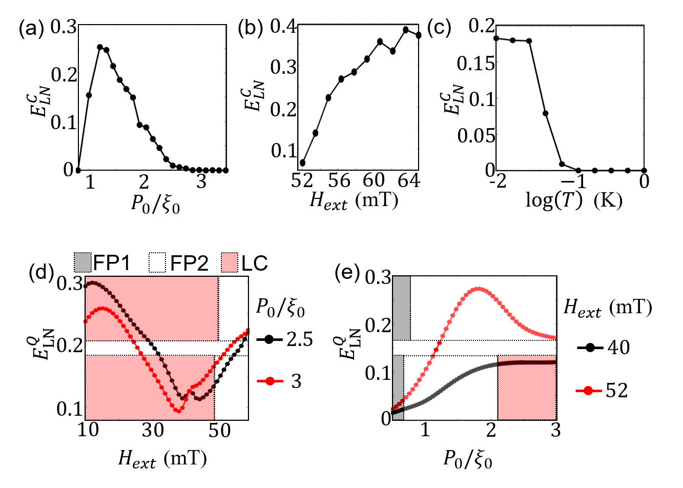
Figure 5: Entanglement. (a)-(c) From semi-classical, (d)-(e) from quantum calculations. (a) Gaussian logarithmic negativity $E_{LN}^{C}$ dependence on $P_{0}/\xi_{{0}}$ for $H_{ext}=52\,$mT and $T=0\,$K. (b) The dependence of $E_{LN}^{C}$ on $H_{ext}$ for $P_{0}/\xi_{0}=2$ and $T=0\,$K. (c) The dependence of $E_{LN}^{C}$ on $T$ for $H_{ext}=52\,$mT and $P_{0}/\xi_{0}=2$. (d) The dependence of logarithmic negativity $E_{LN}^{Q}$, on $H_{ext}$ for two values of $P_{0}/\xi_{0}=2.5,\,3$. (e) The dependence of $E_{LN}^{Q}$ on $P_{0}/\xi_{0}$ for $H_{ext}=40,\,52\,$mT. The scaling coefficient $\mathcal{Q}=5\times 10^{9}$ and $T=0\,$K in (d)-(e). The steady state class from Fig. 2(a) corresponding to each point is shown by color coded rectangles, where top (bottom) rectangles are for red (black) dots.

Quantum entanglement - The driven quantum state is a many-body wave function in which the fluctuations of two types of magnons may become quantum entangled. At the steady-state fixed points of both Kittel and $\vec{\mathcal{K}}_{s}$ modes beyond the Suhl instability threshold, the cross Kerr interaction $c_{0}^{{\dagger}}c_{0}c_{\vec{\mathcal{K}}_{s}}^{{\dagger}}c_{\vec{\mathcal{K}}_{s}}+\mathrm{H.c}.$ can be approximated by $\alpha_{0}^{\ast}\alpha_{\vec{\mathcal{K}}_{s}}^{\ast}\delta c_{0}\delta c_{\vec{\mathcal{K}}_{s}}+\mathrm{H.c}.$, where $\alpha_{0(\vec{\mathcal{K}}_{s})}$ is mean field value of the Kittel ($\vec{\mathcal{K}}_{s}$) mode, and $\delta c$ indicates fluctuations. Under the conditions discussed below, this “two-mode squeezing” term leads to quantum correlations. In the SM Sec. III [38], we discuss the corrections by the “beam-splitter” interaction.

The quantum correlations that characterize entanglement become apparent in the noise statistics. The “quantumness” of the system [41] can be measured by the mean-square fluctuations

$$\sigma=\left\langle\left(\delta x_{0}-\delta x_{\vec{\mathcal{K}}_{s}}\right)^{2}+\left(\delta p_{0}+\delta p_{\vec{\mathcal{K}}_{s}}\right)^{2}\right\rangle=\xi_{0}\frac{n_{\mathrm{th}}+\frac{1}{2}}{2\mathfrak{g}+\xi_{0}}$$ (6)

where $\mathfrak{g}=\left|\mathcal{D}_{0,0,\pm\vec{\mathcal{K}},\pm\vec{\mathcal{K}}}\alpha_{0}^{\ast}\alpha_{\vec{\mathcal{K}}_{s}}^{\ast}\right|$ (see SM Sec. III [38]). In the regime $0\leq\sigma<1/2$, the two modes are necessarily quantum-correlated or “entangled”. When the modes do not interact $\mathfrak{g}=0_{,}$ $\sigma\rightarrow n_{\mathrm{th}}+1/2.$ In general, uncorrelated and classical states correspond to $\sigma\geq 1/2.$ When $\mathfrak{g}$ becomes large, the fluctuations and $\sigma$ vanish, which reflects commutation of the operators for the relative positions and momenta $\left[\delta x_{0}-\delta x_{\vec{\mathcal{K}}_{s}},\delta p_{0}+\delta p_{\vec{\mathcal{K}}_{s}}\right]=0$ in that limit. $\sigma\propto\left(n_{\mathrm{th}}+1/2\right)$ illustrates how increasing temperature destroys quantum correlations by pushing the system into the classical regime $\sigma>1/2\$irrespective of the interactions. This allows us to estimate the experimental conditions to observe quantum entanglement in realistic systems, see below and SM Sec. III [38].

For an accurate assessment of the bipartite quantum entanglement between the Kittel and $\vec{\mathcal{K}}_{s}$ magnons fluctuations all mean-field terms of equal order must be included, which can be done only numerically. Moreover, $\sigma$ is not a good measure of the entanglement resource. More suitable is the “logarithmic negativity” function $E_{LN}\$that increases monotonically with the degree of entanglement [42]. This parameter is measure of the negativity of the partial transposition of the density matrix (with respect to the Kittel mode) $\rho^{PT}=\rho_{0}^{T}\otimes\rho_{\vec{\mathcal{K}}_{s}}$ that vanishes when the bipartite state is separable. $E_{LN}=\text{log}_{2}\left(1+2|\mathfrak{n}|\right)$, where $\mathfrak{n}$ is the sum of the negative eigenvalues of $\rho^{PT}.$ $E_{LN}$ is an upper bound of the “distillable” entanglement $E_{D}$, which is again a measure for the number of completely entangled pairs of quasiparticles (singlets) that can be extracted from the many-body wave function by local operations and classical communications [41, 43, 44], which are essential for e.g. quantum teleportation and quantum key distribution [45, 46, 41, 7]. The density matrix of a Gaussian state, i.e. a localized state in phase space or fixed point, is completely determined by the first and second moments of position and momentum variables, i.e. the covariance matrix, via which $E_{LN}$ can be readily calculated [42, 47] (see SM Sec. III [38]). $E_{LN}=0$ for a separable bipartite state and it diverges for $\sigma=0$. In realistic systems usually $E_{LN}<1$ [49, 48]. Here, we calculate the steady state covariance matrix $\mathcal{V}_{ss}$ by ensemble averaging over 100 independent $50\,\mathrm{\mu}$s runs starting from random initial conditions over the last $1\,\mathrm{\mu}$s. Figures 5(a)-(c) summarize results of the Gaussian logarithmic negativity $E_{LN}^{C}$ calculated via $\mathcal{V}_{ss}$ for some of the FP2 cases identified earlier. Here the superscript $C$ indicates the Gaussian assumption. In Figure 5(a), we observe that $E_{LN}^{C}$ as a function of $P_{0}$, for $H_{\mathrm{ext}}=52\,$mT and zero temperature, is zero below the Suhl instability threshold (at $P_{0}/\xi_{0}=0.92$) and peaks at relatively small $P_{0}$. Figure 5(b) shows that for a fixed $P_{0}/\xi_{0}=2$, $E_{LN}^{C}$ increases strongly with $H_{\mathrm{ext}}$ (see Fig. S5) up to about $\sim 0.5$. According to Figure 5(c) $E_{LN}^{C}$ decreases with increasing $T,$ but remains nearly constant up to $T\approx 100\,$mK. In SM Sec. III and Fig. S3 [38], we support these observations by an analytical analysis.

The entanglement of Gaussian states may be computed by the semi-classical approach. When nonlinearities drive the fluctuations beyond Gaussian statistics, we have to solve the quantum master equation for the steady state density matrix $\rho_{ss}$. The elements of $\rho_{ss}$ correspond to $|i,j\rangle\langle i^{\prime},j^{\prime}|$, where $i$ ($i^{\prime}$) and $j$ ($j^{\prime}$) refer to the $i$’th ($i^{\prime}$’th) and $j$’th ($j^{\prime}$’th) Fock (number) state of the Kittel ($\vec{\mathcal{K}}_{s}$) mode, and we require the sum of the negative eigenvalues of the partially transposed density matrix with elements $|i^{\prime},j\rangle\langle i,j^{\prime}|$. Figure 5(d) shows that $E_{LN}^{Q}$ (superscript Q for quantum) is non-monotonic in $H_{\mathrm{ext}}.$ It turns out to be minimal when the quantum stochasticity $\mathcal{F}_{Q}$ in Figure 4(d) is maximal. The phase space occupied by an LC is much larger than that of the quantum fluctuations, hence distilling the entanglement is not feasible. Therefore, only the entanglement in the FP2 region is useful. Figure 5(d) shows that $E_{LN}^{Q}$ increases with $H_{\mathrm{ext}}$ in the FP2 region, similar to Fig. 5(b). Figure 5(e) shows that with decreasing $P_{0}$ towards FP1 region, $E_{LN}^{Q}$ approaches zero. It can also be seen that it has a peak in $P_{0}$ for $H_{\mathrm{ext}}=52\,$mT similar to Fig. 5(a).

In order to measure and distill the entanglement, both the Kittel mode and the large wave vector magnon pair should resonantly couple to microwaves. This can be achieved by a coplanar waveguide that is modulated with the wave length of the wing magnons that locks the otherwise undetermined phase difference $\phi$ between the $\pm\vec{\mathcal{K}}$ pair, i.e. the nodes of the standing wave magnon amplitude [21].

Conclusion - We study the bistable nature of the Ising spin system emulated by ferromagnetic disk parametrically excited in a microwave cavity as a function of temperature, magnetic field, and excitation power. The Suhl decay of the Kittel mode into a degenerate pair of magnons with large wave vector substantially enhances the random switching between the two energy minima of the Kittel mode parametron phase space, providing a probabilistic bit for stochastic information processing. On the other hand, the Suhl instability is also responsible for a finite distillable entanglement, which is a fundamental resource for quantum information. We show that the three regimes of operation are accessible by varying the parametric excitation power as well as the external magnetic field. The quantum correlations in macroscopic magnets should be observable at low but experimentally accessible temperatures of $\sim$100 mK. We conclude that magnetic particles are attractive building blocks for coherent Ising machines, as well as stochastic and quantum information applications.

Acknowledgments - We acknowledge support by JSPS KAKENHI (Nos. 19H00645 and 21K13847), and JST CREST (No. JPMJCR20C1).

References

- [1] M. Yamaoka, C. Yoshimura, M. Hayashi, T. Okuyama, H. Aoki, and H. Mizuno, “A 20k-Spin Ising Chip to Solve Combinatorial Optimization Problems With CMOS Annealing”, IEEE J. Solid-State Circuits 51, 303 (2015).
- [2] T. Inagaki et al., “Large-scale Ising spin network based on degenerate optical parametric oscillators”, Nat. Phys. 10, 415 (2016).
- [3] T. Inagaki et al., “A coherent Ising machine for 2000-node optimization problems”, Science 354, 603 (2016).
- [4] P. L. McMahon, A. Marandi, Y. Haribara, R. Hamerly, C. Langrock, S. Tamate, T. Inagaki, H. Takesue, S. Utsunomiya, K. Aihara, R. L. Byer, M. M. Fejer, H. Mabuchi, Y. Yamamoto “A fully programmable 100-spin coherent Ising machine with all-to-all connections”, Science 354, 614 (2016).
- [5] D. Pierangeli et al., “Large-Scale Photonic Ising Machine by Spatial Light Modulation”, Phys. Rev. Lett. 122, 213902 (2019).
- [6] W. A. Borders, A. Z. Pervaiz, S. Fukami, K. Y. Camsari, H. Ohno, and S. Datta, “Integer factorization using stochastic magnetic tunnel junctions”, Nature 573, 390 (2019).
- [7] M. A. Nielsen and I. L. Chuang, Quantum computation and quantum information, Cambridge Univ. Press, Cambridge (2009).
- [8] D. P. DiVincenzo, Quantum Computation, Science 270, 255 (1995).
- [9] T. Albash and D. A. Lidar, “Adiabatic quantum computation”, Rev. Mod. Phys. 90, 015002 (2018).
- [10] E. Farhi et al., “A Quantum Adiabatic Evolution Algorithm Applied to Random Instances of an NP-Complete Problem”, Science 292, 472 (2001).
- [11] S. Boixo et al., “Evidence for quantum annealing with more than one hundred qubits”, Nat. Phys. 10, 218 (2014).
- [12] M. W. Johnson, M. H. S. Amin, S. Gildert, T. Lanting, F. Hamze, N. Dickson, R. Harris, A. J. Berkley, J. Johansson, P. Bunyk, E. M. Chapple, C. Enderud, J. P. Hilton, K. Karimi, E. Ladizinsky, N. Ladizinsky, T. Oh, I. Perminov, C. Rich, M. C. Thom, E. Tolkacheva, C. J. S. Truncik, S. Uchaikin, J. Wang, B. Wilson, and G. Rose, “Quantum annealing with manufactured spins”, Nature 473, 194 (2011).
- [13] I. Mahboob, H. Okamoto, and H. Yamaguchi, “An electromechanical Ising Hamiltonian”, Sci. Adv. 2, e1600236 (2016).
- [14] T. Makiuchi, T. Hioki, Y. Shimazu, Y. Oikawa, N. Yokoi, S. Daimon, and E. Saitoh, “Parametron on magnetic dot: Stable and stochastic operation”, Appl. Phys. Lett. 118, 022402 (2021).
- [15] X. Zhang, C.-L. Zou, L. Jiang, and H. X. Tang, Strongly Coupled Magnons and Cavity Microwave Photons, Phys. Rev. Lett. 113, 156401 (2014).
- [16] H. Huebl, C. W. Zollitsch, J. Lotze, F. Hocke, M. Greifenstein, A. Marx, R. Gross, and S. T. B. Goennenwein, High Cooperativity in Coupled Microwave Resonator Ferrimagnetic Insulator Hybrids, Phys. Rev. Lett. 111, 127003 (2013).
- [17] Y. Tabuchi, S. Ishino, T. Ishikawa, R. Yamazaki, K. Usami, and Y. Nakamura, Hybridizing Ferromagnetic Magnons and Microwave Photons in the Quantum Limit, Phys. Rev. Lett. 113, 083603 (2014).
- [18] Y. Tabuchi, S. Ishino, A. Noguchi, T. Ishikawa, R. Yamazaki, K. Usami, and Y. Nakamura, Coherent Coupling Between a Ferromagnetic Magnon and a Superconducting Qubit, Science 349, 405 (2015).
- [19] D. Lachance-Quirion, S. P. Wolski, Y. Tabuchi, S. Kono, K. Usami, and Y. Nakamura, Science 367, 425 (2020).
- [20] J. Li, S.-Y. Zhu, and G. S. Agarwal, Phys. Rev. Lett. 121, 203601 (2018).
- [21] M. Elyasi, Y. M. Blanter, G. E. W. Bauer, Phys. Rev. B 101, 054402 (2020).
- [22] H. Y. Yuan and Rembert A. Duine, Phys. Rev. B 102, 100402 (2020).
- [23] M. Aspelmeyer, T. J. Kippenberg, and F. Marquardt, Cavity Optomechanics, Rev. Mod. Phys. 86, 1391 (2014).
- [24] V. E. Demidov, O. Dzyapko, S. O. Demokritov, G. A. Melkov, and A. N. Slavin, Thermalization of a Parametrically Driven Magnon Gas Leading to Bose-Einstein Condensation, Phys. Rev. Lett. 99, 037205 (2007).
- [25] V. E. Demidov, O. Dzyapko, S. O. Demokritov, G. A. Melkov, and A. N. Slavin, Observation of Spontaneous Coherence in Bose-Einstein Condensate of Magnons, Phys. Rev. Lett. 100, 047205 (2008).
- [26] A. A. Serga, V. S. Tiberkevich, C. W. Sandweg, V. I. Vasyuchka, D. A. Bozhko, A. V. Chumak, T. Neumann, B. Obry, G. A. Melkov, A. N. Slavin, and B. Hillebrands, Bose-Einstein Condensation in an Ultra-Hot Gas of Pumped Magnons, Nat. Commun. 5, 3452 (2013).
- [27] D. A. Bozhko, A. A. Serga, P. Clausen, V. I. Vasyuchka, F. Heussner, G. A. Melkov, A. Pomyalov, V. S. Lvov, and B. Hillebrands, Supercurrent in a Room-Temperature Bose-Einstein Magnon Condensate, Nat. Phys. 12, 1057 (2016).
- [28] H. Suhl, The Theory of Ferromagnetic Resonance at High Signal Powers, Phys. Chem. Solids 1, 209 (1957).
- [29] S. M. Rezende, Theory of Coherence in Bose-Einstein Condensation Phenomena in a Microwave-Driven Interacting Magnon Gas, Phys. Rev. B 79, 174411 (2009).
- [30] B. A. Kalinikos and A. N. Slavin, Theory of Dipole-Exchange Spin Wave Spectrum for Ferromagnetic Films with Mixed Exchange Boundary Conditions, J. Phys. C: Solid State Phys. 19, 7013 (1986).
- [31] M. J. Hurben and C. E. Patton, Theory of Magnetostatic Waves for in-Plane Magnetized Isotropic Films, J. Magn. Magn. Mater. 139, 263 (1995).
- [32] D. D. Stancil and A. Prabhakar, Spin Waves, Springer (2009).
- [33] P. Krivosik and C. E. Patton, “Hamiltonian formulation of nonlinear spin-wave dynamics: Theory and applications”, Phys. Rev. B 82, 184428 (2010).
- [34] S. M. Rezende “Fundamentals of magnonics”, Springer (2020).
- [35] P. Kinsler and P. D. Drummond, “Quantum dynamics of the parametric oscillator”, Phys. Rev. A 43, 6194 (1991).
- [36] H. J. Carmichael, Statistical Methods in Quantum Optics, Springer (1999).
- [37] D. F. Walls and G. J. Milburn, Quantum Optics, Springer (2008).
- [38] See supporting material [URL will be inserted by publisher] for derivation of equations of motion from the master equation, calculation of tunneling frequency from quantum master equation solution, analytical discussion on tunneling frequency of a fixed point parametron, analytical quantification of the Gaussian entanglement, demonstration of limit cycle evolution and doublings, analytical explanation of the steady state phase diagram including the fixed point to limit cycle bifurcation, and correlation of limit cycle oscillation amplitude with Kittel mode parametron tunneling frequency.
- [39] P. H. Bryant, C. D. Jeffries, and K. Nakamura, Spin-Wave Dynamics in a Ferrimagnetic Sphere, Phys. Rev. A 38, 4223 (1988).
- [40] V. E. Zakharov, V. S. L’vov, and S. S. Starobinets, Spin-wave turbulence beyond the parametric excitation threshold, Sov. Phys. Usp. 17, 896 (1974).
- [41] S. L. Braunstein and P. van Loock, Quantum Information with Continuous Variables, Rev. Mod. Phys. 77, 513 (2005).
- [42] G. Vidal and R. F. Werner, Computable Measure of Entanglement, Phys. Rev. A 65, 032314 (2002).
- [43] C. H. Bennett, H. J. Bernstein, S. Popescu, and B. Schumacher, Concentrating Partial Entanglement by Local Operations, Phys. Rev. A 53, 2046 (1996).
- [44] M. Horodecki, P. Horodecki, and R. Horodecki, Inseparable Two Spin- Density Matrices Can Be Distilled to a Singlet Form, Phys. Lett. A 223, 1 (1996).
- [45] S. L. Braunstein, and H. J. Kimble, Teleportation of Continuous Quantum Variables, Phys. Rev. Lett. 80, 869 (1998).
- [46] A. Furusawa, J. L. Sørensen, S. L. Braunstein, C. A. Fuchs, H. J. Kimble, and E. S. Polzik, Unconditional Quantum Teleportation, Science 282, 706 (1998).
- [47] G. Adesso and F. Illuminati, Gaussian Measures of Entanglement versus Negativities: Ordering of Two-Mode Gaussian States, Phys. Rev. A 72, 032334 (2005).
- [48] T. A. Palomaki, J. D. Teufel, R. W. Simmonds, and K. W. Lehnert, Entangling Mechanical Motion with Microwave Fields, Science 342, 710 (2013).
- [49] E. P. Menzel, R. D. Candia, F. Deppe, P. Eder, L. Zhong, M. Ihmig, M. Haeberlein, A. Baust, E. Hoffmann, D. Ballester, K. Inomata, T. Yamamoto, Y. Nakamura, E. Solano, A. Marx, and R. Gross, Path Entanglement of Continuous-Variable Quantum Microwaves, Phys. Rev. Lett. 109 250502 (2012).