Double-RIS Versus Single-RIS Aided Systems: Tensor-Based MIMO Channel Estimation and Design Perspectives

Abstract

Reconfigurable intelligent surfaces (RISs) have been proposed recently as new technology to tune the wireless propagation channels in real-time. However, most of the current works assume single-RIS (S-RIS)-aided systems, which can be limited in some application scenarios where a transmitter might need a multi-RIS-aided channel to communicate with a receiver. In this paper, we consider a double-RIS (D-RIS)-aided MIMO system and propose an alternating least-squared-based channel estimation method by exploiting the Tucker2 tensor structure of the received signals. Using the proposed method, the cascaded MIMO channel parts can be estimated separately, up to trivial scaling factors. Compared with the S-RIS systems, we show that if the RIS elements of a S-RIS system are distributed carefully between the two RISs in a D-RIS system, the training overhead can be reduced and the estimation accuracy can also be increased. Therefore, D-RIS systems can be seen as an appealing approach to further increase the coverage, capacity, and efficiency of future wireless networks compared to S-RIS systems.

Index Terms—  Double RIS, TUCKER2 decomposition, channel estimation, RIS reflection design.

1 Introduction

Reconfigurable intelligent surfaces (RISs) have been proposed recently as a cost-effective technology for reconfiguring the propagation channels in wireless communication systems [1]. An RIS is a 2D surface equipped with a large number of tunable units that can be realized using, e.g., inexpensive antennas or metamaterials and controlled in real-time to influence the communication channels without generating its own signals. Recently, RIS-aided communications have attracted great attention [2], due to their potential of improving the efficiency, the communication range, and the capacity of wireless communication systems.

Most of the current works, e.g., in [3, 4, 5, 6, 7, 8], assume single-RIS (S-RIS)-aided systems, where a transmitter (Tx) communicates with one receiver (Rx), or more, via a single RIS-aided channel. However, in many application scenarios, e.g., in a urban area or in a satellite-to-indoor communication, the Tx might need a multi-RIS-aided channel to have successful communication with the Rx. Moreover, in a S-RIS system, it was shown that the RIS should be either deployed closer to the Tx or closer to the Rx to achieve the best performance gain [9]. This fundamental result gives rise to the double-RIS (D-RIS) systems, where one RIS is deployed closer to the Tx and another is deployed closer to the Rx. In such systems, channel estimation (CE) becomes more problematic since the cascaded (effective) channel contains three parts not only two as in the S-RIS systems (see Fig. 1).

In this paper, we consider a D-RIS aided MIMO system and propose an efficient CE method by exploiting the tensor structure of the received signals [10, 11, 12]. Specifically, we first show that the received signals in flat-fading D-RIS aided MIMO systems can be arranged in a 3-way tensor that admits a Tucker2 decomposition [10]. Accordingly, an alternating least-squared (ALS)-based method is proposed, where the Tx-to-RIS 1 channel (denoted by ${\bf H}_{\text{T}}$), the-RIS 1-to-RIS 2 channel (denoted by ${\bf H}_{\text{S}}$), and the RIS 2-to-Rx channel (denoted by ${\bf H}_{\text{R}}$) can be estimated separately, up to trivial scaling factors. We compare the proposed ALS method for D-RIS systems to the ALS method for S-RIS systems proposed in [8, 7] in terms of the minimum training overhead and the estimation accuracy. It is shown that if the RIS elements in the S-RIS systems are distributed carefully between the two RISs in the D-RIS systems, the training overhead can be reduced and the estimation accuracy can also be increased. Note that, since the system spectral efficiency is inversely proportional to the length of the training overhead, we conjecture that there is an optimal distribution of the RIS elements that strikes an optimal trade-off between the training overhead and the achievable performance, which is out of the scope of this paper and we leave for future work. It is worth mentioning that the considered D-RIS system can also resemble communication scenarios where the RISs in both communicating ends are co-located with the transceivers, as it has been proposed in [13]. Therefore, ${\bf H}_{\text{T}}$ and ${\bf H}_{\text{R}}$ channels can be assumed known by careful transceivers design.

2 D-RIS System Model

In this section, we consider a D-RIS-aided MIMO communication system as depicted on the left-side of Fig. 1, where a Tx with $M_{\text{T}}$ antennas is communicating with a Rx with $M_{\text{R}}$ antennas via a D-RIS-aided channel. Here, RIS 1 is assumed to be close to the Tx and has $N_{1}$ reflecting elements, while RIS 2 is assumed to be close to the Rx and has $N_{2}$ reflecting elements. We assume that the Tx-to-Rx, the Tx-to-RIS 2, and the RIS 1-to-Rx channels are unavailable due to blockage or too weak due to high pathloss.

Let ${\bf H}_{\text{T}}\in\mathbb{C}^{N_{1}\times M_{\text{T}}}$ be the Tx-to-RIS 1 channel, ${\bf H}_{\text{S}}\in\mathbb{C}^{N_{2}\times N_{1}}$ be the RIS 1-to-RIS 2 channel, and ${\bf H}_{\text{R}}\in\mathbb{C}^{M_{\text{R}}\times N_{2}}$ be the RIS 2-to-Rx channel. To estimate these channels, we conduct a channel-training procedure, which occupies $L=I\cdot K$ subframes. The received signal at the $(i,k)$th subframe, $i\in\{1,\dots,I\}$ and $k\in\{1,\dots,K\}$, can be written as

$${\bf\bar{y}}_{i,k}={\bf H}_{\text{R}}\bm{\Phi}_{i}{\bf H}_{\text{S}}\bm{\Psi}_{i}{\bf H}_{\text{T}}{\bf f}_{k}s_{k}+{\bf\bar{n}}_{i,k}\in\mathbb{C}^{M_{\text{R}}},$$ (1)

where $\bm{\Psi}_{i}=\text{diag}\{\bm{\psi}_{i}\}\in\mathbb{C}^{N_{1}\times N_{1}}$ is the $i$th diagonal reflection matrix of RIS 1, with $\bm{\psi}_{i}\in\mathbb{C}^{N_{1}}$ and $|[\bm{\psi}_{i}]_{[j]}|=1/\sqrt{N_{1}}$, $\bm{\Phi}_{i}=\text{diag}\{\bm{\phi}_{i}\}\in\mathbb{C}^{N_{2}\times N_{2}}$ is the $i$th diagonal reflection matrix of RIS 2, with $\bm{\phi}_{i}\in\mathbb{C}^{N_{2}}$ and $|[\bm{\phi}_{i}]_{[j]}|=1/\sqrt{N_{2}}$, ${\bf f}_{k}\in\mathbb{C}^{M_{\text{T}}}$ is the $k$th precoding vector at the Tx with $\|{\bf f}_{k}\|=1$, $s_{k}$ is the $k$th unit-norm training symbol, and ${\bf\bar{n}}_{i,k}\in\mathbb{C}^{M_{\text{R}}}$ is the additive white Gaussian noise vector having zero-mean circularly symmetric complex-valued entries with variance $\sigma^{2}$.

Let $\bm{\Psi}=[\bm{\psi}_{1},\dots,\bm{\psi}_{I}]\in\mathbb{C}^{N_{1}\times I}$, $\bm{\Phi}=[\bm{\phi}_{1},\dots,\bm{\phi}_{I}]\in\mathbb{C}^{N_{2}\times I}$, and ${\bf F}=[{\bf f}_{1}s_{1},\dots,{\bf f}_{K}s_{K}]\in\mathbb{C}^{M_{\text{T}}\times K}$. Then, by staking $\{{\bf\bar{y}}_{i,k}\}_{k=1}^{K}$ next to each other as ${\bf\bar{Y}}_{i}=[{\bf\bar{y}}_{i,1},\dots,{\bf\bar{y}}_{i,K}]$, the obtained measurement matrix ${\bf\bar{Y}}_{i}$ can be expressed as

$${\bf\bar{Y}}_{i}={\bf H}_{\text{R}}\bm{\Phi}_{i}{\bf H}_{\text{S}}\bm{\Psi}_{i}{\bf H}_{\text{T}}{\bf F}+{\bf\bar{N}}_{i}\in\mathbb{C}^{M_{\text{R}}\times K},$$ (2)

where ${\bf\bar{N}}_{i}\in\mathbb{C}^{M_{\text{R}}\times K}$ is expressed similarly. We assume that the training matrix ${\bf F}$ is designed with orthonormal rows so that ${\bf F}{\bf F}^{\mathsf{H}}={\bf I}_{M_{\text{T}}}$, which directly implies that $K\geq M_{\text{T}}$. Then, after right filtering ${\bf\bar{Y}}_{i}$ with ${\bf F}^{\mathsf{H}}$, i.e., ${\bf Y}_{i}={\bf\bar{Y}}_{i}{\bf F}^{\mathsf{H}}$, we can write the obtained matrix ${\bf Y}_{i}$ as

$${\bf Y}_{i}={\bf H}_{\text{R}}\bm{\Phi}_{i}{\bf H}_{\text{S}}\bm{\Psi}_{i}{\bf H}_{\text{T}}+{\bf N}_{i}\in\mathbb{C}^{M_{\text{R}}\times M_{\text{T}}},$$ (3)

where ${\bf N}_{i}={\bf\bar{N}}_{i}{\bf F}^{\mathsf{H}}$. Given the measurement matrices ${\bf Y}_{i},\forall i\in\{1,\dots,I\}$, our main goal in Section 2.1 is to obtain an estimate to the channel matrices ${\bf H}_{\text{R}}$, ${\bf H}_{\text{T}}$, and ${\bf H}_{\text{S}}$.

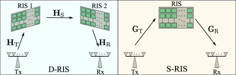
Fig. 1: D-RIS versus S-RIS aided MIMO communications.

2.1 Proposed Tucker2-based for CE in D-RIS systems

By concatenating ${\bf Y}_{1},\dots,{\bf Y}_{I}$ in (3) behind each other, a 3-way tensor can be obtained as $\bm{\mathcal{Y}}=[{\bf Y}_{1},\sqcup_{3}\dots,\sqcup_{3}{\bf Y}_{I}]\in\mathbb{C}^{M_{\text{R}}\times M_{\text{T}}\times I}$, where ${\bf Y}_{i}$ represents its $i$th frontal slice. Here, we note that the tensor $\bm{\mathcal{Y}}$ has a Tucker2 representation as [11]

$$\bm{\mathcal{Y}}=\bm{\mathcal{S}}\times_{1}{\bf H}_{\text{R}}\times_{2}{\bf H}^{\mathsf{T}}_{\text{T}}+\bm{\mathcal{N}}\in\mathbb{C}^{M_{\text{R}}\times M_{\text{T}}\times I},$$ (4)

where $\bm{\mathcal{N}}$ is the noise tensor and $\bm{\mathcal{S}}$ is formed by concatenating $\bm{\Phi}_{i}{\bf H}_{\text{S}}\bm{\Psi}_{i},\forall i\in\{1,\dots,I\}$, behind each other as

$$\bm{\mathcal{S}}=[\bm{\Phi}_{1}{\bf H}_{\text{S}}\bm{\Psi}_{1},\sqcup_{3}\dots,\sqcup_{3}\bm{\Phi}_{I}{\bf H}_{\text{S}}\bm{\Psi}_{I}]\in\mathbb{C}^{N_{\text{2}}\times N_{\text{1}}\times I}.$$ (5)

From the above, the CE problem can be formulated as

$$\{{\bf\hat{H}}_{\text{R}},{\bf\hat{H}}_{\text{T}},{\bf\hat{H}}_{\text{S}}\}=\underset{{\bf H}_{\text{R}},{\bf H}_{\text{T}},{\bf H}_{\text{S}}}{\arg\min}\|\bm{\mathcal{Y}}-\bm{\mathcal{S}}\times_{1}{\bf H}_{\text{R}}\times_{2}{\bf H}^{\mathsf{T}}_{\text{T}}\|^{2}_{\text{F}},$$ (6)

which is nonconvex due to its joint optimization. To obtain a solution, we resort to an alternating minimization approach, where we solve (6) for one variable assuming the other two are fixed. To achieve this end, we exploit the $n$-mode unfoldings of $\bm{\mathcal{Y}}$, i.e., $[\bm{\mathcal{Y}}]_{(n)},n\in\{1,2,3\}$ expressed as [11, 10]

$$[\bm{\mathcal{Y}}]_{(1)} ={\bf H}_{\text{R}}~{}{\bf Z}_{\text{R}}({{\bf H}_{\text{T}}},{{\bf H}_{\text{S}}})+[\bm{\mathcal{N}}]_{(1)}\in\mathbb{C}^{M_{\text{R}}\times IM_{\text{T}}}$$ (7)

$$[\bm{\mathcal{Y}}]_{(2)} ={\bf H}^{\mathsf{T}}_{\text{T}}~{}{\bf Z}_{\text{T}}({{\bf H}_{\text{R}}},{{\bf H}_{\text{S}}})+[\bm{\mathcal{N}}]_{(2)}\in\mathbb{C}^{M_{\text{T}}\times IM_{\text{R}}}$$ (8)

$$[\bm{\mathcal{Y}}]_{(3)} =[\bm{\mathcal{S}}]_{(3)}({\bf H}^{\mathsf{T}}_{\text{T}}\otimes{\bf H}_{\text{R}})^{\mathsf{T}}+[\bm{\mathcal{N}}]_{(3)}\in\mathbb{C}^{I\times M_{\text{T}}M_{\text{R}}},$$ (9)

where ${\bf Z}_{\text{R}}({{\bf H}_{\text{T}}},{{\bf H}_{\text{S}}})=[\bm{\mathcal{S}}]_{(1)}({\bf I}_{I}\otimes{\bf H}^{\mathsf{T}}_{\text{T}})^{\mathsf{T}}\in\mathbb{C}^{N_{\text{2}}\times IM_{\text{T}}}$ and ${\bf Z}_{\text{T}}({{\bf H}_{\text{R}}},{{\bf H}_{\text{S}}})=[\bm{\mathcal{S}}]_{(2)}({\bf I}_{I}\otimes{\bf H}_{\text{R}})^{\mathsf{T}}\in\mathbb{C}^{N_{\text{1}}\times IM_{\text{R}}}$. Note that, according to the definition of $n$-mode unfoldings [10], $[\bm{\mathcal{S}}]_{(3)}\in\mathbb{C}^{I\times N_{\text{1}}N_{\text{2}}}$ can be expressed as $[\bm{\mathcal{S}}]_{(3)}=(\bm{\Psi}\diamond\bm{\Phi})^{\mathsf{T}}\text{diag}\{{\bf h}_{\text{S}}\}$, where ${\bf h}_{\text{S}}=\text{vec}\{{\bf H}_{\text{S}}\}\in\mathbb{C}^{N_{\text{1}}N_{\text{2}}}$. Therefore, we have

$$[\bm{\mathcal{Y}}]_{(3)}=(\bm{\Psi}\diamond\bm{\Phi})^{\mathsf{T}}\text{diag}\{{\bf h}_{\text{S}}\}({\bf H}^{\mathsf{T}}_{\text{T}}\otimes{\bf H}_{\text{R}})^{\mathsf{T}}+[\bm{\mathcal{N}}]_{(3)}.$$ (10)

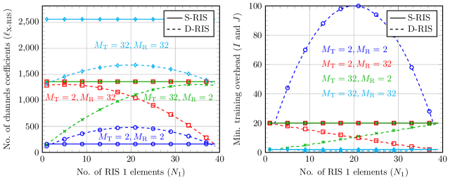
Fig. 2: Number of channels coefficients ($\ell_{\text{X-RIS}}$) and minimum training overhead ($I$ and $J$) [$N=40$, $N_{2}=N-N_{1}$].

The vectorized form of $[\bm{\mathcal{Y}}]_{(3)}$, i.e., ${\bf y}_{(3)}=\text{vec}\{[\bm{\mathcal{Y}}]_{(3)}\}$ can be expressed as

$${\bf y}_{(3)}={\bf Z}_{\text{S}}({{\bf H}_{\text{T}}},{{\bf H}_{\text{R}}})~{}{\bf h}_{\text{S}}+{\bf n}_{(3)}\in\mathbb{C}^{IM_{\text{T}}M_{\text{R}}},$$ (11)

where ${\bf n}_{(3)}=\text{vec}\{[\bm{\mathcal{N}}]_{(3)}\}$ , ${\bf Z}_{\text{S}}({{\bf H}_{\text{T}}},{{\bf H}_{\text{R}}})=\Big{(}({\bf H}^{\mathsf{T}}_{\text{T}}\otimes{\bf H}_{\text{R}})\diamond(\bm{\Psi}\diamond\bm{\Phi})^{\mathsf{T}}\Big{)}\in\mathbb{C}^{IM_{\text{R}}M_{\text{T}}\times N_{\text{1}}N_{\text{2}}}$. By exploiting (7), (8), and (11), an estimate of ${\bf H}_{\text{R}}$, ${\bf H}_{\text{T}}$, and ${\bf h}_{\text{S}}$ can be obtained as

$${\bf\hat{H}}_{\text{R}} =\underset{{\bf H}_{\text{R}}}{\arg\min}\|[\bm{\mathcal{Y}}]_{(1)}-{\bf H}_{\text{R}}~{}{\bf Z}_{\text{R}}({{\bf H}_{\text{T}}},{{\bf H}_{\text{S}}})\|^{2}_{\text{F}}$$ (12)

$${\bf\hat{H}}_{\text{T}} =\underset{{\bf H}_{\text{T}}}{\arg\min}\|[\bm{\mathcal{Y}}]_{(2)}-{\bf H}^{\mathsf{T}}_{\text{T}}~{}{\bf Z}_{\text{T}}({{\bf H}_{\text{R}}},{{\bf H}_{\text{S}}})\|^{2}_{\text{F}}$$ (13)

$${\bf\hat{h}}_{\text{S}} =\underset{{\bf h}_{\text{S}}}{\arg\min}\|{\bf y}_{(3)}-{\bf Z}_{\text{S}}({{\bf H}_{\text{T}}},{{\bf H}_{\text{R}}})~{}{\bf h}_{\text{S}}\|^{2}_{\text{2}}.$$ (14)

The above problems are convex and can be solved using the alternating least squares (ALS) method, as summarized in Algorithm 1, which is guaranteed to converge monotonically to, at least, a locally optimal solution [11].

Algorithm 1 ALS method for CE in D-RIS MIMO systems

1:Input: Measurement tensor $\bm{\mathcal{Y}}\in\mathbb{C}^{M_{\text{R}}\times M_{\text{T}}\times I}$ as in (4)

2:Initialize: ${{\bf H}^{(0)}_{\text{T}}}$ and ${{\bf H}^{(0)}_{\text{S}}}$ and select $t_{\max}$.

3:for $t=1$ to $t_{\max}$ do

4:     ${{\bf H}^{(t)}_{\text{R}}}=[\bm{\mathcal{Y}}]_{(1)}\{{\bf Z}_{\text{R}}({{\bf H}^{(t-1)}_{\text{T}}},{{\bf H}^{(t-1)}_{\text{S}}})\}^{+}$

5:     ${\bf\hat{H}}^{(t)}_{\text{T}}=\big{(}[\bm{\mathcal{Y}}]_{(2)}\{{\bf Z}_{\text{T}}({{\bf H}^{(t)}_{\text{R}}},{{\bf H}^{(t-1)}_{\text{S}}})\}^{+}\big{)}^{\mathsf{T}}$

6:     ${{\bf\hat{H}}^{(t)}_{\text{S}}}=\text{unvec}\Big{\{}\{{\bf Z}_{\text{S}}({{\bf H}^{(t)}_{\text{T}}},{{\bf H}^{(t)}_{\text{R}}})\}^{+}{\bf y}_{(3)}\Big{\}}$

7:end for

3 Comparison with S-RIS aided systems

In S-RIS-aided systems, on the other hand, the communication between the Tx and the Rx with $M_{\text{T}}$ and $M_{\text{R}}$ antennas, respectively, is aided via a single RIS with $N$ elements, as depicted on the right-side of Fig. 1. Let ${\bf G}_{\text{T}}\in\mathbb{C}^{N\times M_{\text{T}}}$ be the Tx to RIS channel and ${\bf G}_{\text{R}}\in\mathbb{C}^{M_{\text{R}}\times N}$ be the RIS to Rx channel. Then, it was shown in [8, 7] that the received signals at the Rx can be arranged in a 3-way tensor admitting a canonical polyadic (CP) decomposition given as

$$\bm{\mathcal{X}}=\bm{\mathcal{I}}_{3,N}\times_{1}{\bf G}_{\text{R}}\times_{2}{\bf G}^{\mathsf{T}}_{\text{T}}\times_{3}\bm{\Omega}^{\mathsf{T}}+\bm{\mathcal{E}}\in\mathbb{C}^{M_{\text{R}}\times M_{\text{T}}\times J},$$ (15)

where $\bm{\mathcal{I}}_{3,N}\in\mathbb{Z}^{N\times N\times N}$ is the super-diagonal tensor, $\bm{\mathcal{E}}$ is the noise tensor, $\bm{\Omega}=[\bm{\omega}_{1},\dots,\bm{\omega}_{J}]\in\mathbb{C}^{N\times J}$ is the RIS training matrix with $J$ training beams and $|[\bm{\omega}_{j}]_{[\ell]}|=1/\sqrt{N}$. The $n$-mode unfoldings of $\bm{\mathcal{X}}$, $n\in\{1,2\}$, can be expressed as

$$[\bm{\mathcal{X}}]_{(1)} ={\bf G}_{\text{R}}~{}{\bf V}_{\text{R}}({\bf G}_{\text{T}})+[\bm{\mathcal{E}}]_{(1)}\in\mathbb{C}^{M_{\text{R}}\times JM_{\text{T}}}$$ (16)

$$[\bm{\mathcal{X}}]_{(2)} ={\bf G}^{\mathsf{T}}_{\text{T}}~{}{\bf V}_{\text{T}}({\bf G}_{\text{R}})+[\bm{\mathcal{E}}]_{(2)}\in\mathbb{C}^{M_{\text{T}}\times JM_{\text{R}}},$$ (17)

where ${\bf V}_{\text{R}}({\bf G}_{\text{T}})=(\bm{\Omega}^{\mathsf{T}}\diamond{\bf G}^{\mathsf{T}}_{\text{T}})^{\mathsf{T}}\in\mathbb{C}^{N\times JM_{\text{T}}}$ and ${\bf V}_{\text{T}}({\bf G}_{\text{R}})=(\bm{\Omega}^{\mathsf{T}}\diamond{\bf G}_{\text{R}})^{\mathsf{T}}\in\mathbb{C}^{N\times JM_{\text{R}}}$. Therefore, an ALS-based method, similarly to Algorithm 1, has been proposed in [8] to obtain an estimate of ${\bf G}_{\text{R}}$ and ${\bf G}_{\text{T}}$, as summarized in Algorithm 2.

Algorithm 2 ALS method for CE in S-RIS MIMO systems

1:Input: Measurement tensor $\bm{\mathcal{X}}\in\mathbb{C}^{M_{\text{R}}\times M_{\text{T}}\times J}$ as in (15)

2:Initialize: ${{\bf G}^{(0)}_{\text{T}}}$ and select $t_{\max}$.

3:for $t=1$ to $t_{\max}$ do

4:     ${{\bf G}^{(t)}_{\text{R}}}=[\bm{\mathcal{X}}]_{(1)}\{{\bf V}_{\text{R}}({\bf G}^{(t-1)}_{\text{T}})\}^{+}$

5:     ${{\bf G}^{(t)}_{\text{T}}}=\big{(}[\bm{\mathcal{X}}]_{(2)}\{{\bf V}_{\text{T}}({\bf G}^{(t)}_{\text{R}})\}^{+}\big{)}^{\mathsf{T}}$

6:end for

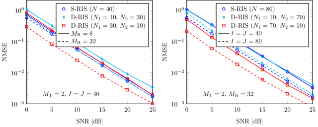
Fig. 3: NMSE versus SNR comparing the D-RIS against the S-RIS systems for different system settings [$M_{\text{T}}=2$].

Identifiablity, in the LS sense, can be obtained by noting that ${\bf Z}_{\text{R}}$, ${\bf Z}_{\text{T}}$, ${\bf V}_{\text{R}}$, and ${\bf V}_{\text{T}}$ need to have full column-rank, while ${\bf Z}_{\text{S}}$ needs to have full row-rank [11]. This leads to the following conditions: $IM_{\text{T}}\geq N_{\text{2}}$ (for ${\bf Z}_{\text{R}}$), $IM_{\text{R}}\geq N_{\text{1}}$ (for ${\bf Z}_{\text{T}}$), $JM_{\text{T}}\geq N$ (for ${\bf V}_{\text{R}}$), $JM_{\text{R}}\geq N$ (for ${\bf V}_{\text{T}}$), and $IM_{\text{R}}M_{\text{T}}\geq N_{\text{1}}N_{\text{2}}$ (for ${\bf Z}_{\text{S}}$). Therefore, we conclude that

$$I \geq\max\big{\{}\left\lceil{N_{\text{2}}}/{M_{\text{T}}}\right\rceil,~{}~{}\left\lceil{N_{\text{1}}}/{M_{\text{R}}}\right\rceil,~{}~{}\left\lceil{N_{\text{1}}N_{\text{2}}}/{M_{\text{R}}M_{\text{T}}}\right\rceil\big{\}}$$ (18)

$$J \geq\max\big{\{}\left\lceil{N}/{M_{\text{T}}}\right\rceil,~{}~{}\left\lceil{N}/{M_{\text{R}}}\right\rceil\big{\}},$$ (19)

where (18) is for the D-RIS systems and (19) is for the S-RIS systems. Let $\ell_{\text{D-RIS}}$ and $\ell_{\text{S-RIS}}$ denote the total number of channel coefficients in the D-RIS and the S-RIS communication scenarios, respectively, which are given as

$$\ell_{\text{D-RIS}} =M_{\text{T}}N_{1}+N_{1}N_{2}+M_{\text{R}}N_{2}$$ (20)

$$\ell_{\text{S-RIS}} =M_{\text{T}}N+M_{\text{R}}N.$$ (21)

Let us assume that the S-RIS elements $N$ are distributed between RIS 1 and RIS 2 in the D-RIS scenario such that $N=N_{1}+N_{2}$. In Fig. 2 we plot results of (18), (19), (20), and (21) for different $M_{\text{R}}$ and $M_{\text{T}}$ values assuming $N=40$. Note that along the $x$-axis we vary $N_{1}$ so that $N_{2}=N-N_{1}$. From Fig. 2, we have the following remarks:

Remark 1: If $N\gg\max\{{M_{\text{R}}},{M_{\text{T}}}\}$ and ${M_{\text{R}}}\approx{M_{\text{T}}}$, then S-RIS, i.e., Algorithm 2 requires less training overhead compared to D-RIS, i.e., Algorithm 1, in most of the $N_{1}$ and $N_{2}$ distribution scenarios. This comes from the fact that the number of channel coefficients that D-RIS needs to estimate, i.e., $\ell_{\text{D-RIS}}$ is much larger than that of S-RIS, i.e., $\ell_{\text{S-RIS}}$.

Remark 2: If $N\approx\max\{{M_{\text{R}}},{M_{\text{T}}}\}$, then D-RIS requires less training overhead compared to S-RIS for the same reason mentioned in Remark 1, i.e., $\ell_{\text{D-RIS}}<\ell_{\text{S-RIS}}$.

Remark 3: In the D-RIS systems, the careful distribution of the $N$ elements between RIS 1 and RIS 2 (i.e., $N_{1}$ and $N_{2}$) can reduce the training overhead of Algorithm 1. From Fig. 2, we can note that the best distribution depends on the ${M_{\text{R}}}$ and the ${M_{\text{T}}}$ values as: if ${M_{\text{R}}}>{M_{\text{T}}}$, then it is more beneficial to allocate more elements to RIS 1 than RIS 2, i.e., $N_{1}>N_{2}$. This observation is reversed if ${M_{\text{R}}}<{M_{\text{T}}}$, i.e., more elements should be allocated to RIS 2 than RIS 1 as $N_{1}<N_{2}$.

Computational complexity: Assuming that the conditions in (18) and (19) are satisfied, the complexities of Algorithm 1 and Algorithm 2 are on the order of $\mathcal{O}\big{(}t_{\max}\cdot(N^{3}_{2}+N^{3}_{1}+(N_{1}\cdot N_{2})^{3})\big{)}$ and $\mathcal{O}\big{(}t_{\max}\cdot 2N^{3}\big{)}$, respectively.

Ambiguities: Assuming that the conditions in (18) and (19) are satisfied, then the estimated MIMO channels by Algorithm 1 and Algorithm 2 are unique up to scalar ambiguities [8, 11]. In particular, the estimated channels are related to the perfect (true) channels as: ${\bf\hat{H}}_{\text{R}}\approx{\bf H}_{\text{R}}\bm{\Delta}_{\text{R}}$, ${\bf\hat{H}}_{\text{T}}\approx\bm{\Delta}_{\text{T}}{\bf H}_{\text{T}}$, ${\bf H}_{\text{S}}\approx\bm{\Delta}^{-1}_{\text{R}}{\bf\hat{H}}_{\text{S}}\bm{\Delta}^{-1}_{\text{T}}$, ${\bf\hat{G}}_{\text{R}}\approx{\bf G}_{\text{R}}\bm{\Lambda}$, and ${\bf\hat{G}}_{\text{T}}\approx\bm{\Lambda}^{-1}{\bf\hat{G}}_{\text{T}}$, where $\bm{\Delta}$ and $\bm{\Lambda}$ are diagonal matrices holding the scaling ambiguities. However, these ambiguities disappear when reconstructing an estimate of the effective end-to-end channels ${\bf\hat{H}}_{\text{e}}={\bf\hat{H}}_{\text{R}}{\bf\hat{H}}_{\text{S}}{\bf\hat{H}}_{\text{T}}$ and ${\bf\hat{G}}_{\text{e}}={\bf\hat{G}}_{\text{R}}{\bf\hat{G}}_{\text{T}}$. Moreover, note that, due to the knowledge of the RIS reflection matrices $\bm{\Psi}$, $\bm{\Phi}$, and $\bm{\Omega}$ at the Rx, the permutation ambiguities do not exist [8].

4 Simulation Results

We assume that the entries of the channel matrices ${\bf H}_{\text{R}}$, ${\bf H}_{\text{T}}$, ${\bf H}_{\text{S}}$, ${\bf G}_{\text{R}}$, and ${\bf G}_{\text{T}}$ follow a Rayleigh fading distribution. We show results in terms of the normalized-mean-square-error (NMSE) of the effective channels defined as $\text{NMSE}=\mathbb{E}\big{\{}{\|{\bf H}_{\text{e}}-{{\bf\hat{H}}}_{\text{e}}\|^{2}_{\text{F}}\big{\}}}/\mathbb{E}\big{\{}{\|{\bf H}_{\text{e}}\|^{2}_{\text{F}}}\big{\}}$, for the D-RIS, and $\text{NMSE}=\mathbb{E}\big{\{}{\|{\bf G}_{\text{e}}-{{\bf\hat{G}}}_{\text{e}}\|^{2}_{\text{F}}\big{\}}}/\mathbb{E}\big{\{}{\|{\bf G}_{\text{e}}\|^{2}_{\text{F}}}\big{\}}$, for the S-RIS. We define the signal-to-noise ratio (SNR) as $\text{SNR}=\mathbb{E}\big{\{}{\|\bm{\mathcal{Y}}-\bm{\mathcal{N}}\|^{2}_{\text{F}}}\big{\}}/\mathbb{E}\big{\{}{\|\bm{\mathcal{N}}\|^{2}_{\text{F}}}\big{\}}$, for the D-RIS, and $\text{SNR}=\mathbb{E}\big{\{}{\|\bm{\mathcal{X}}-\bm{\mathcal{E}}\|^{2}_{\text{F}}}\big{\}}/\mathbb{E}\big{\{}{\|\bm{\mathcal{E}}\|^{2}_{\text{F}}}\big{\}}$, for the S-RIS. Moreover, assuming that $I\leq N_{1}N_{2}$ and $J\leq N$, the training matrices ${\bf\Psi}$, ${\bf\Phi}$, and ${\bm{\Omega}}$ are updated using a DFT-based approach as: ${\bf\Phi}=[{\bf W}_{N_{2}}\otimes\bm{1}^{\mathsf{T}}_{\bar{I}_{2}}]_{[:,1:I]}$, ${\bf\Psi}=[\bm{1}^{\mathsf{T}}_{\bar{I}_{1}}\otimes{\bf W}_{N_{1}}]_{[:,1:I]}$, and ${\bm{\Omega}}=[{\bf W}_{N}]_{[:,1:J]}$, where $\bar{I}_{1}=\left\lceil\frac{I}{N_{1}}\right\rceil$, $\bar{I}_{2}=\left\lceil\frac{I}{N_{2}}\right\rceil$, and ${\bf W}_{K}$ is the normalized $K\times K$ DFT matrix such that ${\bm{\Omega}}^{\mathsf{H}}{\bm{\Omega}}={\bf I}_{J}$ and $\bm{\Upsilon}^{\mathsf{H}}\bm{\Upsilon}={\bf I}_{I}$, where $\bm{\Upsilon}\stackrel{{\scriptstyle\mathclap{\mbox{\tiny def}}}}{{=}}\bm{\Psi}\diamond\bm{\Phi}$.

Fig. 3 shows the NMSE versus SNR results for different system settings. From the left-side figure, we can see that when $M_{\text{R}}=8$, the D-RIS, i.e., Algorithm 1 has a worse NMSE performance compared to the S-RIS, i.e., Algorithm 2 especially with the $[N_{1},N_{2}]=[10,30]$ distribution scenario. This can be explained from Fig. 2 and Remarks 1 and 3. Note that in a such system setting, the D-RIS has a larger number of channels coefficients $\ell_{\text{D-RIS}}=560$ compared to the S-RIS $\ell_{\text{S-RIS}}=400$. Moreover, as we have highlighted in Remark 3, we can see that the $[N_{1},N_{2}]=[30,10]$ distribution scenario has a better NMSE performance than $[N_{1},N_{2}]=[10,30]$, since $M_{\text{T}}<M_{\text{R}}$. On the other hand, when $M_{\text{R}}=32$, we can see that the D-RIS has a much better NMSE performance compared to the S-RIS, especially with the $[N_{1},N_{2}]=[30,10]$ distribution scenario. This can be explained in the same way from Fig. 2 and Remarks 2 and 3. From the right-side figure, we can see that the same observations hold true when we increase $N$ from $40$ to $80$ or when we increase the training overhead $I$ and $J$ from $40$ to $80$.

5 Conclusions

In this paper, we have shown that D-RIS MIMO systems can be used to reduce the training overhead and to improve the channel estimation accuracy compared to S-RIS aided systems. This comes from the observation that if the RIS elements in the S-RIS system are distributed carefully between the two RISs in the D-RIS system, the number of channel coefficients in the D-RIS system that need to be estimated reduces significantly compared to the S-RIS system. Therefore, D-RIS systems can be seen as an appealing approach to further increase the coverage, capacity, and efficiency of wireless networks compared to S-RIS systems.

References

• [1] C. Liaskos, S. Nie, A. Tsioliaridou, A. Pitsillides, S. Ioannidis, and I. Akyildiz, “A new wireless communication paradigm through software-controlled metasurfaces,” IEEE Commun. Mag., vol. 56, no. 9, pp. 162–169, 2018.
• [2] M. Di Renzo, A. Zappone, M. Debbah, M.-S. Alouini, C. Yuen, J. de Rosny, and S. Tretyakov, “Smart radio environments empowered by reconfigurable intelligent surfaces: How it works, state of research, and the road ahead,” IEEE J. Sel. Areas Commun., vol. 38, no. 11, pp. 2450–2525, 2020.
• [3] S. Zhang and R. Zhang, “Capacity characterization for intelligent reflecting surface aided MIMO communication,” IEEE J. Sel. Areas Commun., vol. 38, no. 8, pp. 1823–1838, Aug. 2020.
• [4] K. Ardah, S. Gherekhloo, A. L. F. de Almeida, and M. Haardt, “TRICE: A channel estimation framework for RIS-aided millimeter-wave MIMO systems,” IEEE Signal Process. Lett., vol. 28, pp. 513–517, Feb. 2021.
• [5] S. Gherekhloo, K. Ardah, A. L. de Almeida, and M. Haardt, “Tensor-based channel estimation and reflection design for RIS-aided millimeter-wave MIMO communication systems,” arXiv preprint arXiv:2107.13851, 2021.
• [6] Q. Wu and R. Zhang, “Intelligent reflecting surface enhanced wireless network via joint active and passive beamforming,” IEEE Trans. Wireless Commun., vol. 18, no. 11, pp. 5394–5409, 2019.
• [7] G. T. de Araújo and A. L. F. de Almeida, “PARAFAC-based channel estimation for intelligent reflective surface assisted MIMO system,” in Proc. IEEE 11th Sensor Array and Multichannel Signal Processing Workshop (SAM), 2020, pp. 1–5.
• [8] G. T. de Araújo, A. L. F. de Almeida, and R. Boyer, “Channel estimation for intelligent reflecting surface assisted MIMO systems: A tensor modeling approach,” IEEE J. Sel. Topics Signal Process., vol. 15, no. 3, pp. 789–802, 2021.
• [9] E. Björnson and L. Sanguinetti, “Power scaling laws and near-field behaviors of massive MIMO and intelligent reflecting surfaces,” IEEE Open J. Commun. Soc., vol. 1, pp. 1306–1324, 2020.
• [10] T. G. Kolda and B. W. Bader, “Tensor decompositions and applications,” SIAM Review, vol. 51, no. 3, pp. 455–500, Sept. 2009.
• [11] P. Comon, X. Luciani, and A. L. F. de Almeida, “Tensor decompositions, alternating least squares and other tales,” Journal of Chemometrics, vol. 23, no. 7-8, pp. 393–405, 2009.
• [12] K. Ardah, A. L. F. de Almeida, and M. Haardt, “Low-complexity millimeter wave CSI estimation in MIMO-OFDM hybrid beamforming systems,” in Proc. 23rd International ITG Workshop on Smart Antennas (WSA), Apr. 2019, pp. 1–5.
• [13] V. Jamali, A. M. Tulino, G. Fischer, R. R. Müller, and R. Schober, “Intelligent surface-aided transmitter architectures for millimeter-wave ultra massive MIMO systems,” IEEE Open J. Commun. Soc., vol. 2, pp. 144–167, 2021.