Relaxed Conditions for Parameterized Linear Matrix Inequality in the Form of Double Sum

Do Wan Kim and Dong Hwan Lee D. W. Kim is with the Department of Electrical Engineering, Hanbat National University, Deajeon, Korea, e-mail: dowankim@hanbat.ac.kr.D. H. Lee is with the Department of Electrical Engineering, KAIST, Deajeon, Korea, e-mail: donghwan@kaist.ac.kr.
Abstract

The aim of this study is to investigate less conservative conditions for a parameterized linear matrix inequality (PLMI) expressed in the form of a double convex sum. This type of PLMI frequently appears in T-S fuzzy control system analysis and design problems. In this letter, we derive new, less conservative linear matrix inequalities (LMIs) for the PLMI by employing the proposed sum relaxation method based on Young’s inequality. The derived LMIs are proven to be less conservative than the existing conditions related to this topic in the literature. The proposed technique is applicable to various stability analysis and control design problems for T-S fuzzy systems, which are formulated as solving the PLMIs in the form of a double convex sum. Furthermore, examples is provided to illustrate the reduced conservatism of the derived LMIs.

Index Terms:
T-S fuzzy system, relaxed condition, parameterized linear matrix inequality (PLMI), linear matrix inequality (LMI)

I Introduction

Parameterized Linear Matrix Inequalities (PLMIs) play a significant role in various fields, including T-S fuzzy control [1, 2, 3, 4, 5, 6, 7, 8, 9] and robust control [10, 11, 12, 13, 14, 15, 16]. These PLMIs are utilized in control design and analysis problems, where the objective is to find matrix variables that satisfy the PLMIs over infinite-dimensional parameter spaces. This problem, referred to as a PLMI problem (PLMIP) in this letter, poses challenges due to its infinite-dimensional nature, making it generally numerically intractable.

To address this challenge, researchers have made efforts to derive finite-dimensional sufficient linear matrix inequality (LMI) conditions for PLMIPs. For instance, several studies such as [10, 11, 12] proposed sufficient LMI conditions for PLMIPs expressed as single convex sums (or fuzzy sums) of matrices. In these approaches, the matrices in the fuzzy sum vary within a matrix polytope as parameters change. Additionally, works such as [2, 3, 13, 4, 14, 5, 6, 7] developed sufficient LMI conditions for PLMIPs expressed as double fuzzy sums. Moreover, techniques based on Polya’s theorem [17] have been employed to extend these conditions to triple fuzzy sums [8] and more general $N$ fuzzy sums [9, 15]. These sufficient conditions typically evaluate PLMIs at finite vertices of matrix polytopes, which cover the corresponding parameterized matrix space. The idea behind improving these conditions is to express matrix polytopes with finer and tighter vertex grids, and then verify the PLMIs at these vertices. This approach leads to less conservative conditions, reflecting the main concept of generalization based on Polya’s theorem.

In this letter, our primary focus is on the sufficient LMI condition presented in [2] for PLMIs expressed as a double fuzzy sum. This particular condition, as described in [2], incorporates distinct over-bounding techniques and employs different types of vertices compared to other existing works. It is well-known for producing less conservative results in numerous problem scenarios. The effectiveness of this sufficient condition has led to its widespread adoption within the field of fuzzy control, as shown in studies such as [7]. However, despite its initial development in 2001, to the best of our knowledge, its full potential has yet to be fully explored in subsequent research over the past few decades.

Motivated by the preceding discussion, the primary objective of this letter is to investigate less conservative LMI conditions for PLMIPs expressed as double fuzzy sums. This is achieved by extending the concepts introduced in [2]. Specifically, we propose a novel sufficient LMI condition for PLMIPs using Young’s inequality. The newly developed LMI condition encompasses the condition presented in [2] as a special case. Theoretical analysis confirms that our proposed condition is less conservative than the one in [2]. Additionally, our approach offers a clear and simplified analysis framework and proof for the condition in [2] by leveraging Young’s inequality, which can be generalized to PLMIPs with multiple fuzzy sum forms. The proposed technique is applicable to various control design problems in the context of T-S fuzzy systems represented by PLMIs formulated as double fuzzy sums. Furthermore, examples are included to demonstrate the decreased conservatism of the derived LMIs.

Notations: The notation $P\succ Q$ ($P\prec Q$) denotes that the matrix $P-Q$ is positive (negative) definite. In this context, $\mathbb{R}$ represents the set of real numbers, $\mathbb{R}^{n}$ denotes the $n$-dimensional Euclidean space, and $\mathbb{R}^{m\times n}$ refers to the field of real matrices with dimensions $m\times n$. Furthermore, $\mathbb{I}_{r}$ represents the integer set $\{1,2,\ldots,r\}$ where $r>1$. To simplify notation, we will use $x$ instead of $x(t)$ for continuous-time signal vectors unless otherwise specified.

II Problem Formulation

Consider the PLMI in the form of a double fuzzy sum:

$\displaystyle\Phi(z)=\sum_{i=1}^{r}\sum_{j=1}^{r}h_{i}(z)h_{j}(z)\Phi_{ij}\prec 0$ (1)

Here, $z\in\mathbb{R}^{p}$ represents the premise variable, $h_{i}(z):\mathscr{D}_{z}~{}\rightarrow\mathbb{R}_{[0,1]}$ satisfies $\sum_{i=1}^{r}h_{i}(z)=1$, $\mathscr{D}_{z}\subset\mathbb{R}^{p}$ denotes the domain of the premise variables, and $\Phi_{ij}=\Phi_{ij}^{T}\in\mathbb{R}^{n\times n},$ $(i,j)\in\mathbb{I}_{r}\times\mathbb{I}_{r}$ is a matrix that may have a linear dependency on the decision variables. The PLMI (1) commonly arises in controller designs or stability analyses of linear uncertain models [16] and T-S fuzzy systems [2, 5, 18]. The sufficient LMIs for negativeness, $\Phi_{ij}\prec 0$, $(i,j)\in\mathbb{I}_{r}\times\mathbb{I}_{r}$, can be derived straightforwardly by omitting $h_{i}h_{j}\in\mathbb{R}_{>0}$. Various efforts have been made to provide less conservative LMI conditions for the PLMI (1) in the form of a double fuzzy sum. Initially, relaxation techniques [2, 5] were introduced, utilizing the properties of double fuzzy sums, such as $\sum_{i=1}^{r}\sum_{j=1}^{r}h_{i}h_{j}\Phi_{ij}=\sum_{i=1}^{r}h_{i}^{2}\Phi_{ii}+\sum_{i=1}^{r}\sum_{j=1,j>i}^{r}h_{i}h_{j}(\Phi_{ij}+\Phi_{ji})$. These sum relaxations [2, 5] serve as the foundation for subsequent researches, including the introduction of slack variables [3, 4] and the extension of multidimensional summations [9] (for more details, see [19]). As stated in [6, 7], the following lemma [2] is one of popular LMI conditions:

Lemma 1 (Theorem 2.2 of [2])

The PLMI (1) holds if

$\displaystyle\Phi_{ii}$ $\displaystyle\prec 0,\quad\forall i\in\mathbb{I}_{r}$
$\displaystyle\frac{2}{r-1}\Phi_{ii}+\Phi_{ij}+\Phi_{ji}$ $\displaystyle\prec 0,\quad\forall(i,j)\in\{(i,j)\in\mathbb{I}_{r}\times\mathbb{I}_{r}~{}|~{}i\neq j\}.$

Lemma 1 will play a crucial role in this letter, as we develop a new LMI condition that includes it as a special case. In particular, the problems of interest in this letter is to develop less conservative LMI conditions which generalize those in Lemma 1 and prove their less conservatism.

III Main Results

Before presenting our main results, we introduce the following lemmas, which will be used throughout the letter:

Lemma 2 (Young’s inequality [17])

For $a\in\mathbb{R}_{\geqslant 0}$ and $b\in\mathbb{R}_{\geqslant 0}$, $ab\leq\frac{1}{2}{a^{2}}+\frac{1}{2}{b^{2}}$ holds.

Lemma 3

For any matrix $\Xi_{ij}$, $(i,j)\in\left\{\left.(i,j)\in\mathbb{I}_{r}\times\mathbb{I}_{r}~{}\right|~{}j\neq i\right\}$, it is true that

$\displaystyle\sum_{i=1}^{r}\sum_{j=1,j\neq i}^{r}h_{i}^{2}(\Xi_{ij}+\Xi_{ji})=\sum_{i=1}^{r}\sum_{j=1,j\neq i}^{r}h_{j}^{2}(\Xi_{ij}+\Xi_{ji}).$
Proof:

See Appendix A

Now, we are ready to present our main result. In the following theorem, we present a new relaxed LMI condition using Young’s inequality, that generalizes Lemma 1.

Theorem 1

The PLMI (1) holds if

$\displaystyle\Phi_{ii}+\frac{1}{2}\sum\limits_{j=1,j<i}^{r}{\delta_{j}}(\Phi_{ij}+\Phi_{ji})+\frac{1}{2}\sum\limits_{j=1,j>i}^{r}{\delta_{j-1}}(\Phi_{ij}+\Phi_{ji})\prec 0$ (2)

for all $i\in{\mathbb{I}}_{r}$ and all

$$(\delta_{1},\delta_{2},\ldots,\delta_{r-1})\in\underbrace{\{0,1\}\times\{0,1\}\times\cdots\times\{0,1\}}_{(r-1)-{\rm{times}}}.$$
Proof:

It is obvious that PLMI (1)xTΦ(z)x<0,xn,x0PLMI (1)formulae-sequencesuperscript𝑥𝑇Φ𝑧𝑥0formulae-sequencefor-all𝑥superscript𝑛𝑥0\textrm{PLMI \eqref{eq: PLMI}}\Leftrightarrow x^{T}\Phi(z)x<0,\forall x\in\mathbb{R}^{n},x\neq 0. We can equivalently rewrite $x^{T}\Phi(z)x$ as

$\displaystyle x^{T}\Phi(z)x$ $\displaystyle=\sum_{i=1}^{r}{h_{i}^{2}x^{T}\Phi_{ii}x}+\frac{1}{2}\sum_{i=1}^{r}\sum_{j=1,j\neq i}^{r}h_{i}h_{j}x^{T}(\Phi_{ij}+\Phi_{ji})x$

If $x^{T}(\Phi_{ij}+\Phi_{ji})x\geq 0$ on the right-hand side in the above equation, then since $h_{i}h_{j}x^{T}(\Phi_{ij}+\Phi_{ji})x\geq 0$, applying Lemma 2 to $h_{i}h_{j}x^{T}(\Phi_{ij}+\Phi_{ji})x$ yields

$\displaystyle h_{i}h_{j}x^{T}(\Phi_{ij}+\Phi_{ji})x\leq\frac{1}{2}\left(h_{i}^{2}+h_{j}^{2}\right)x^{T}(\Phi_{ij}+\Phi_{ji})x$

Otherwise, if $x^{T}(\Phi_{ij}+\Phi_{ji})x<0$, then $h_{i}h_{j}x^{T}(\Phi_{ij}+\Phi_{ji})x\leq 0$. By considering both cases, we have

$\displaystyle h_{i}h_{j}x^{T}(\Phi_{ij}+\Phi_{ji})x$ $\displaystyle\leq\max\left\{\frac{1}{2}\left(h_{i}^{2}+h_{j}^{2}\right)x^{T}(\Phi_{ij}+\Phi_{ji})x,0\right\}$
$\displaystyle=\frac{1}{2}\left(h_{i}^{2}+h_{j}^{2}\right)\max\left\{x^{T}(\Phi_{ij}+\Phi_{ji})x,0\right\}.$

With this inequality, it can be shown that

$\displaystyle x^{T}\Phi(z)x\leq$ $\displaystyle\sum_{i=1}^{r}{h_{i}^{2}x^{T}\Phi_{ii}x}$
$\displaystyle+\frac{1}{4}\sum_{i=1}^{r}\sum_{j=1,j\neq i}^{r}\left(h_{i}^{2}+h_{j}^{2}\right)\max\left\{x^{T}(\Phi_{ij}+\Phi_{ji})x,0\right\}.$

Using Lemma 3, we obtain

$\displaystyle x^{T}\Phi(z)x$
$\displaystyle\quad\leq\sum_{i=1}^{r}{h_{i}^{2}x^{T}\Phi_{ii}x}+\frac{1}{2}\sum_{i=1}^{r}\sum_{j=1,j\neq i}^{r}h_{i}^{2}\max\left\{x^{T}(\Phi_{ij}+\Phi_{ji})x,0\right\}$
$\displaystyle\quad=\sum_{i=1}^{r}h_{i}^{2}\left(x^{T}\Phi_{ii}x+\frac{1}{2}\sum_{j=1,j\neq i}^{r}\max\left\{x^{T}(\Phi_{ij}+\Phi_{ji})x,0\right\}\right).$

To avoid $\max$ operator on the right-hand side, we can consider all possible cases, which leads to the desired conclusion:

LMIs (2)xTΦ(z)x<0,xn,x0PLMI (1)\displaystyle\textrm{LMIs \eqref{eq: propose LMI}}\Rightarrow x^{T}\Phi(z)x<0,\forall x\in{\mathbb{R}}^{n},x\neq 0\Leftrightarrow\textrm{PLMI \eqref{eq: PLMI} }

Lemma 1 is based on the positive definiteness property of a 2-by-2 matrix within the nonnegative orthant. In contrast, the proposed sufficient condition employs a different bounding approach utilizing Young’s inequality. Consequently, conducting a direct and intuitive comparison between the two may not be feasible. However, we can demonstrate that the proposed Theorem 1 is less conservative than Lemma 1. The utilization of Young’s inequality, which provides more flexibility in calculating the new bounds, is the main factor contributing to the relaxation.

Corollary 1

The LMI condition (2) of Theorem 1 is less conservative than the LMI condition of Lemma 1.

Proof:

To prove the claim about conservatism, we show that the LMIs of Lemma 1 imply LMIs (2) of Theorem 1, while the converse is not true. First, one can prove that the LMIs of Lemma 1 implies

$$\frac{2}{{r-1}}\Phi_{ii}+\delta_{k}(\Phi_{ij}+\Phi_{ji})\prec 0,\quad\forall i\in{\mathbb{I}}_{r},k\in\{1,2,\ldots,r-1\}$$

for all $\delta_{k}\in\{0,1\},k\in\{1,2,\ldots,r-1\}$. This is because when $\delta_{k}=1$, the above LMI becomes the second LMI in Lemma 1, and when $\delta_{k}=0$, the above LMI becomes the first LMI in Lemma 1. Next, letting

$$k=k(j)=\left\{{\begin{array}[]{*{20}c}j,&j<i;\\ j-1,&{\rm{otherwise}}\\ \end{array}}\right.$$

in the foregoing inequality and summing both sides of the foregoing inequality over $j\in\mathbb{I}_{r},j\neq i$ lead to (2). Therefore, this proves that if the LMIs of of Lemma 1 are feasible, then so are the LMIs in (2).

Next, we provide an example for which the LMIs in (2) are feasible, while the LMIs of Lemma 1 are not feasible. Consider the case that $r=3$, $\Phi_{11}=-2$, $\Phi_{22}=-1$, $\Phi_{33}=-2$, $\Phi_{12}=0$, $\Phi_{13}=2$, $\Phi_{21}=0$, $\Phi_{23}=-1$, $\Phi_{31}=0$, and $\Phi_{32}=0$. Then, LMIs (2) of Theorem 1 are satisfied as follows: $\Phi_{11}+\sum_{j=1,j<1}^{3}{\delta_{j}}\frac{{\Phi_{1j}+\Phi_{j1}}}{2}+\sum_{j=1,j>1}^{3}{\delta_{j-1}}\frac{{\Phi_{1j}+\Phi_{j1}}}{2}$ is $\Phi_{11}=-2$ when $(\delta_{1},\delta_{2})=(0,0)$, $\Phi_{11}+\frac{\Phi_{13}+\Phi_{31}}{2}=-0.5$ when $(\delta_{1},\delta_{2})=(0,1)$, $\Phi_{11}+\frac{\Phi_{12}+\Phi_{21}}{2}=-2$ when $(\delta_{1},\delta_{2})=(1,0)$, $\Phi_{11}+\sum_{j=1,j\neq 1}^{3}\frac{\Phi_{1j}+\Phi_{j1}}{2}=-0.5$ when $(\delta_{1},\delta_{2})=(1,1)$. For $\Phi_{22}+\sum_{j=1,j<2}^{3}{\delta_{j}}\frac{{\Phi_{2j}+\Phi_{j2}}}{2}+\sum_{j=1,j>2}^{3}{\delta_{j-1}}\frac{{\Phi_{2j}+\Phi_{j2}}}{2}$, it is equal to $\Phi_{22}=-1$ when $(\delta_{1},\delta_{2})=(0,0)$, $\Phi_{22}+\frac{\Phi_{23}+\Phi_{32}}{2}=-1.5$ when $(\delta_{1},\delta_{2})=(0,1)$, $\Phi_{22}+\frac{\Phi_{21}+\Phi_{12}}{2}=-1$ when $(\delta_{1},\delta_{2})=(1,0)$, $\Phi_{22}+\sum_{j=1,j\neq 2}^{3}\frac{\Phi_{2j}+\Phi_{j2}}{2}=-1.5$ when $(\delta_{1},\delta_{2})=(1,1)$. Lastly, for $\Phi_{33}+\sum_{j=1,j<3}^{3}{\delta_{j}}\frac{{\Phi_{3j}+\Phi_{j3}}}{2}+\sum_{j=1,j>3}^{3}{\delta_{j-1}}\frac{{\Phi_{3j}+\Phi_{j3}}}{2}$, it is equal to $\Phi_{33}=-2$ when $(\delta_{1},\delta_{2})=(0,0)$, $\Phi_{33}+\frac{\Phi_{32}+\Phi_{23}}{2}=-2.5$ when $(\delta_{1},\delta_{2})=(0,1)$, $\Phi_{33}+\frac{\Phi_{31}+\Phi_{13}}{2}=-0.5$ when $(\delta_{1},\delta_{2})=(1,0)$, $\Phi_{33}+\sum_{j=1,j\neq 3}^{3}\frac{\Phi_{3j}+\Phi_{j3}}{2}=-1$ when $(\delta_{1},\delta_{2})=(1,1)$. On the other hand, the LMIs of Lemma 1 are infeasible because $\frac{2}{{r-1}}\Phi_{11}+\Phi_{13}+\Phi_{31}=-2+2+0=0$. This completes the proof.

Corollary 1 establishes that Theorem 1 is not more conservative than Lemma 1 by demonstrating that the condition in Lemma 1 implies the condition in Theorem 1. Furthermore, it proves the less conservativeness of Theorem 1 compared to Lemma 1 by presenting a counterexample for which the condition of Theorem 1 is feasible while the condition of Lemma 1 is not.

Remark 1

We emphasize that

  1. 1.

    When $r=2$, LMIs (2) of Theorem 1 are equal to those of Lemma 1.

  2. 2.

    Both Lemma 1 and Theorem 1 need no additional slack variables.

  3. 3.

    Lemma 1 still plays an important role when sufficient LMIs are derived from PLMI (1) in the form of the double convex sum (see, for example, [20, 21, 22], and references therein). However, Theorem 1 shows that LMIs of Lemma 1 are sufficient to ensure that LMIs (2) of Theorem 1 hold; hence, Theorem 1 could be substituted for Lemma 1.

Remark 2

The numerical complexity of optimization problems based on LMIs can be estimated by considering the total number of scalar decision variables, denoted as $N_{D}$, and the total row size of the LMIs, denoted as $N_{L}$ [23]. For the LMIs in Lemma 1 and Theorem 1, the number of scalar decision variables depends on the specific problem at hand. Therefore, we focus solely on the total row size $N_{L}$ of the LMIs. In Lemma 1, we have $N_{L}=n\times r^{2}$, whereas in Theorem 1, we have $N_{L}=n\times r\times 2^{r-1}$. It is worth noting that the total row size grows exponentially as $r$ increases. Hence, the numerical complexity of Theorem 1 is greater than that of Lemma 1, particularly when $r$ is large. This increased complexity can be regarded as a cost to pay for the relaxation.

Remark 3

Lemma 1 relies on the positive definiteness property of a 2-by-2 matrix within the nonnegative orthant. Consequently, generalizing this condition to triple and more general $N$ fuzzy summation cases is challenging due to the need for considering the positive definiteness property of general matrices, which are inherently more complex. On the other hand, the proposed approach is based on Young’s inequality, enabling a more straightforward generalization to cases involving more general $N$ fuzzy summations. Although the general $N$ fuzzy summations encompass a broader range of applications, it is worth noting that the simple double fuzzy summation case still encapsulates the core ideas. Considering these generalizations is deferred to potential future topics.

IV Examples

All numerical examples in this letter were treated with the help of MATLAB 2020a running on a Windows 10 PC with AMD Ryzen 3970X 3.69G Hz CPU, 128 GB RAM. The LMI problems were solved with MATLAB LMI Control Toolbox [23].

Example 1

Consider the asymptotic stabilization condition [5] for continuous-time T-S fuzzy systems in the form of PLMI (1) with

$\displaystyle\Phi_{ij}=(A_{i}Q+B_{i}F_{j})^{T}+A_{i}Q+B_{i}F_{j},\quad(i,j)\in\mathbb{I}_{3}\times\mathbb{I}_{3}$

widely used for the fuzzy control system

$\displaystyle\dot{x}=\sum_{i=1}^{3}h_{i}(A_{i}x+B_{i}u),\quad u=\sum_{i=1}^{3}h_{i}F_{i}Q^{-1}x,$

where $Q=Q^{T}\succ 0$ and $F_{i}$ are the matrix variables to be determined, $A_{i}$ and $B_{i}$ borrowed from [8] are

$\displaystyle A_{1}=$ $\displaystyle\begin{bmatrix}1.59&-7.29\\ 0.01&0\end{bmatrix},B_{1}=\begin{bmatrix}1\\ 0\end{bmatrix},$
$\displaystyle A_{2}=$ $\displaystyle\begin{bmatrix}0.02&-4.64\\ 0.35&0.21\end{bmatrix},B_{2}=\begin{bmatrix}8\\ 0\end{bmatrix},$
$\displaystyle A_{3}=$ $\displaystyle\begin{bmatrix}-a&-4.33\\ 0&0.\end{bmatrix},B_{3}=\begin{bmatrix}-b+6\\ -1\end{bmatrix}.$

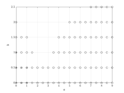
We change the values of the nonnegative parameters $a$ and $b$ to check the feasibility of LMIs of Lemma 1 and Theorem 1. Figure 1 shows the feasible points $(a,b)$ for Lemma 1 and Theorem 1, respectively. Here, the mark ‘$\circ$’ indicates that the LMI of Theorem 1 is feasible, and the mark ‘$\times$’ denotes that the LMI of Lemma 1 is feasible. As discussed in Theorem 1, one can see that Theorem 1 provides less conservative results than Lemma 1.

Refer to caption
Figure 1: Example : Stabilizable region by Theorem 1 (‘$\circ$’) and Lemma 1 (‘$\times$’)
Example 2

Consider the discrete-time T-S fuzzy control system

$\displaystyle x(k+1)=$ $\displaystyle\sum_{i=1}^{3}h_{i}(A_{i}x(k)+B_{i}u(k)),$
$\displaystyle u(k)=$ $\displaystyle\sum_{i=1}^{3}h_{i}F_{i}Q^{-1}x(k),$

where $Q=Q^{T}\succ 0$ and $F_{i}$ are the matrix variables to be determined, $A_{i}=I+\tilde{A}_{i}T$, $B_{i}=\tilde{B}_{i}T$ for $i\in\mathbb{I}_{3}$, $T=0.4$, and

$\displaystyle\tilde{A}_{1}=$ $\displaystyle\begin{bmatrix}2&-10\\ 1&0\end{bmatrix},\tilde{B}_{1}=\begin{bmatrix}1\\ 0\end{bmatrix},$
$\displaystyle\tilde{A}_{2}=$ $\displaystyle\begin{bmatrix}a&-10\\ 1&0\end{bmatrix},\tilde{B}_{2}=\begin{bmatrix}b\\ 0\end{bmatrix},$
$\displaystyle\tilde{A}_{3}=$ $\displaystyle\begin{bmatrix}-2&-10\\ 1&0\end{bmatrix},\tilde{B}_{3}=\begin{bmatrix}1\\ 0.334\end{bmatrix}$

borrowed from [24]. The asymptotic stabilization condition [5] takes the PLMI form (1) with

$\displaystyle\Phi_{ij}=\begin{bmatrix}-Q&(A_{i}Q+B_{i}F_{j})^{T}\\ A_{i}Q+B_{i}F_{j}&-Q\end{bmatrix}.$

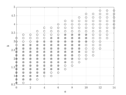
We find the feasible regions of Lemma 2 and Theorem 1 by varying the values of nonnegative $a$ and $b$. Figure 2 depicts the feasible points $(a,b)$, where the mark ‘$\times$’ and ‘$\circ$’ are for Lemma 2 and Theorem 1, respectively. As shown Figure 2, we see that the feasible region of Theorem 1 is larger than that of Lemma 2.

Refer to caption
Figure 2: Example  Stabilizable region by Theorem 1 (‘$\circ$’) and Lemma 1 (‘$\times$’)

V Conclusions

This letter presents new sufficient conditions for PLMIs formulated as a double convex sum. These conditions are expressed in LMIs, derived without the need for slack variables. Moreover, the less conservative nature of these conditions has been rigorously demonstrated. Theoretical claims put forth in this work have been effectively validated through experimental results. Potential avenues for future research include generalizing the LMI conditions for general $N$ convex summations. Additionally, conducting a comparative analysis between the proposed frameworks and slack variable approaches documented in the literature presents an interesting prospect for further investigation.

Finally, it is worth noting that although this letter specifically focuses on double fuzzy sum cases, the concept can be readily extended to encompass triple and more general $N$ fuzzy sum cases, albeit with increased complexity. However, expanding the analysis to these scenarios significantly complicates the main analysis, which exceeds the scope of this letter. Moreover, it has the potential to obscure the fundamental ideas and insights of our proposed approach. Hence, this letter restricts its scope to the double fuzzy sum scenarios, and we defer the exploration of these extensions to future research, as they hold promising possibilities for further investigation.

Appendix A Proof of Lemma 3

It is not hard to see that

$\displaystyle\sum_{i=1}^{r}\sum_{j=1,j\neq i}^{r}h_{i}^{2}(\Phi_{ij}+\Phi_{ji})$
$\displaystyle=\sum_{i=1}^{r}\sum_{j=1,j\neq i}^{r}(h_{i}^{2}-h_{j}^{2})(\Phi_{ij}+\Phi_{ji})+\sum_{i=1}^{r}\sum_{j=1,j\neq i}^{r}h_{j}^{2}(\Phi_{ij}+\Phi_{ji})$
$\displaystyle=\sum_{i=1}^{r}\sum_{j=1,j>i}^{r}(h_{i}^{2}-h_{j}^{2})(\Phi_{ij}+\Phi_{ji})$
$\displaystyle\quad+\sum_{i=1}^{r}\sum_{j=1,j<i}^{r}(h_{i}^{2}-h_{j}^{2})(\Phi_{ij}+\Phi_{ji})+\sum_{i=1}^{r}\sum_{j=1,j\neq i}^{r}h_{j}^{2}(\Phi_{ij}+\Phi_{ji})$
$\displaystyle=\sum_{i=1}^{r}\sum_{j=1,j>i}^{r}(h_{i}^{2}-h_{j}^{2})(\Phi_{ij}+\Phi_{ji})$
$\displaystyle\quad-\sum_{i=1}^{r}\sum_{j=1,j>i}^{r}(h_{i}^{2}-h_{j}^{2})(\Phi_{ij}+\Phi_{ji})+\sum_{i=1}^{r}\sum_{j=1,j\neq i}^{r}h_{j}^{2}(\Phi_{ij}+\Phi_{ji})$
$\displaystyle=\sum_{i=1}^{r}\sum_{j=1,j\neq i}^{r}h_{j}^{2}(\Phi_{ij}+\Phi_{ji}).$

References

  • [1] L. Kong and J. Yuan, “New relaxed stabilization conditions for discrete-time Takagi–Sugeno fuzzy control systems,” Asian Journal of Control, vol. 22, no. 4, pp. 1604–1616, 2020.
  • [2] H. D. Tuan, P. Apkarian, T. Narikiyo, and Y. Yamamoto, “Parameterized linear matrix inequality techniques in fuzzy control system design,” IEEE Transactions on fuzzy systems, vol. 9, no. 2, pp. 324–332, 2001.
  • [3] E. Kim and H. Lee, “New approaches to relaxed quadratic stability condition of fuzzy control systems,” IEEE Transactions on Fuzzy systems, vol. 8, no. 5, pp. 523–534, 2000.
  • [4] M. C. Teixeira, E. Assunção, and R. G. Avellar, “On relaxed LMI-based designs for fuzzy regulators and fuzzy observers,” IEEE Transactions on Fuzzy Systems, vol. 11, no. 5, pp. 613–623, 2003.
  • [5] H. O. Wang and K. Tanaka, Fuzzy control systems design and analysis: a linear matrix inequality approach.   John Wiley & Sons, 2004.
  • [6] T.-M. Guerra, A. Kruszewski, L. Vermeiren, and H. Tirmant, “Conditions of output stabilization for nonlinear models in the Takagi–Sugeno’s form,” Fuzzy Sets and Systems, vol. 157, no. 9, pp. 1248–1259, 2006.
  • [7] J.-T. Pan, T. M. Guerra, S.-M. Fei, and A. Jaadari, “Nonquadratic stabilization of continuous T–S fuzzy models: LMI solution for a local approach,” IEEE Transactions on Fuzzy Systems, vol. 20, no. 3, pp. 594–602, 2011.
  • [8] C.-H. Fang, Y.-S. Liu, S.-W. Kau, L. Hong, and C.-H. Lee, “A new LMI-based approach to relaxed quadratic stabilization of TS fuzzy control systems,” IEEE Transactions on fuzzy systems, vol. 14, no. 3, pp. 386–397, 2006.
  • [9] A. Sala and C. Ariño, “Asymptotically necessary and sufficient conditions for stability and performance in fuzzy control: Applications of Polya’s theorem,” Fuzzy sets and systems, vol. 158, no. 24, pp. 2671–2686, 2007.
  • [10] M. C. De Oliveira, J. Bernussou, and J. C. Geromel, “A new discrete-time robust stability condition,” Systems & control letters, vol. 37, no. 4, pp. 261–265, 1999.
  • [11] D. Peaucelle, D. Arzelier, O. Bachelier, and J. Bernussou, “A new robust $d$-stability condition for real convex polytopic uncertainty,” Systems & control letters, vol. 40, no. 1, pp. 21–30, 2000.
  • [12] M. C. De Oliveira, J. C. Geromel, and J. Bernussou, “Extended $h_{2}$ and $h_{\infty}$ norm characterizations and controller parametrizations for discrete-time systems,” International journal of control, vol. 75, no. 9, pp. 666–679, 2002.
  • [13] D. C. Ramos and P. L. Peres, “An LMI condition for the robust stability of uncertain continuous-time linear systems,” IEEE Transactions on Automatic Control, vol. 47, no. 4, pp. 675–678, 2002.
  • [14] V. J. Leite and P. L. Peres, “An improved LMI condition for robust $d$-stability of uncertain polytopic systems,” IEEE Transactions on Automatic Control, vol. 48, no. 3, pp. 500–504, 2003.
  • [15] R. C. Oliveira and P. L. Peres, “Parameter-dependent LMIs in robust analysis: Characterization of homogeneous polynomially parameter-dependent solutions via LMI relaxations,” IEEE Transactions on Automatic Control, vol. 52, no. 7, pp. 1334–1340, 2007.
  • [16] A.-T. Nguyen, P. Chevrel, and F. Claveau, “Gain-scheduled static output feedback control for saturated LPV systems with bounded parameter variations,” Automatica, vol. 89, pp. 420–424, 2018.
  • [17] G. H. Hardy, J. E. Littlewood, G. Pólya, G. Pólya et al., Inequalities.   Cambridge university press, 1952.
  • [18] K. D. Wan, H. J. Lee, and M. Tomizuka, “Fuzzy stabilization of nonlinear systems under sampled-data feedback: an exact discrete-time model approach,” IEEE Transactions on Fuzzy Systems, vol. 18, no. 2, pp. 251–260, 2010.
  • [19] A.-T. Nguyen, T. Taniguchi, L. Eciolaza, V. Campos, R. Palhares, and M. Sugeno, “Fuzzy control systems: Past, present and future,” IEEE Computational Intelligence Magazine, vol. 14, no. 1, pp. 56–68, 2019.
  • [20] A. Tapia, M. Bernal, and L. Fridman, “Nonlinear sliding mode control design: An LMI approach,” Systems & Control Letters, vol. 104, pp. 38–44, 2017.
  • [21] L. J. Elias, F. A. Faria, R. Araujo, and V. A. Oliveira, “Stability analysis of Takagi–Sugeno systems using a switched fuzzy Lyapunov function,” Information Sciences, vol. 543, pp. 43–57, 2021.
  • [22] F. Li, W. X. Zheng, and S. Xu, “Finite-time fuzzy control for nonlinear singularly perturbed systems with input constraints,” IEEE Transactions on Fuzzy Systems, vol. 30, no. 6, pp. 2129–2134, 2021.
  • [23] P. Gahinet, “Lmi control toolbox,” The Math Works Inc., 1996.
  • [24] A. Sala and C. Arino, “Relaxed stability and performance conditions for Takagi–Sugeno fuzzy systems with knowledge on membership function overlap,” IEEE Transactions on Systems, Man, and Cybernetics, Part B (Cybernetics), vol. 37, no. 3, pp. 727–732, 2007.