Instability of Holographic Superfluids in Optical Lattice

Abstract

The instability of superfluids in optical lattice has been investigated using the holographic model. The static and steady flow solutions are numerically obtained from the static equations of motion and the solutions are described as Bloch waves with different Bloch wave vector $k$. Based on these Bloch waves, the instability is investigated at two levels. At the linear perturbation level, we show that there is a critical $k_{c}$ above which the superflow is unstable. At the fully nonlinear level, the intermediate state and final state of unstable superflow are identified through numerical simulation of the full equations of motion. The results show that during the time evolution, the unstable superflow will undergo a chaotic state with soliton generation. The system will settle down to a stable state with $k<k_{c}$ eventually, with a smaller current and a larger condensate.

I Introduction

As an artificial lattice structure, optical lattice, has a close physical resemblance to the periodic coulomb potential that felt by electrons in solid crystal. While it is not like electrons moving between positive ions in a nanometer dimension, optical lattice can be manipulated with a typical dimension much larger than the conventional crystal—micrometer dimension. Due to this virtue, optical lattice has provided a broad platform for experimental and theoretical physicists to explore much richer and more fundamental properties in condensed matter physics, such as instability PhysRevA.64.061603 ; Wu_2003 , Landau-Zener tunneling 1996PhRvL..76.4504N ; 2000PhRvA..61b3402W ; 2002PhRvA..65f3612C ; 2003PhRvL..91w0406J ; Wu_2003 ; 2020PhRvL.125u3401G , superfluid-Mott insulator quantum phase transition 1998PhRvL..81.3108J ; 2002PhRvA..66c1601K ; 2002PhRvL..89q0402S ; 2004PhRvA..70d3612C ; 2005PhRvA..71d3601Z ; 2006PhRvA..73b3610C and so on. Additionally, by controlling the frequency of the lasers in the course of time, the time-dependent optical lattice can be used for driving the system to explore the floquet dynamics 2015AdPhy..64..139B ; PhysRevLett.115.205301 ; PhysRevLett.121.233603 ; PhysRevX.9.011047 ; 2019NatPh..15.1168S , which are getting more interesting recently.

The instability (or stability) of superfluids is always one of the most fundamental and important properties and usually many physical phenomena are related with it. Since the optical lattice starts to be used for studying cold atom physics, many kinds of research works about the instability have been carried out in various respects. There are Landau or dynamical instability 2001PhRvE..64e6615B ; 2001PhRvE..63c6612B ; PhysRevA.64.061603 ; 2003NJPh….5…71C ; Wu_2003 ; 2004PhRvL..93n0406F ; 2004PhRvA..70d3625M ; PhysRevLett.95.180403 ; PhysRevLett.95.110403 ; 2006PhRvA..74e3611I ; 2006JPhB…39S.101K ; 2007PhRvA..75c3621H ; ZHANG20081147 ; 2009ChPhL..26a6701L ; 2014JPSJ…83l4001A ; PhysRevA.93.013628 ; PhysRevLett.86.4447 ; Cataliotti_2003 ; PhysRevLett.93.140406 ; PhysRevA.72.013603 ; Konabe_2006 , parametric instabilities 2004JPhB…37S.257R ; 2005PhRvA..71f1602K ; 2005PhRvL..95q0404G ; 2017PhRvX…7b1015L ; PhysRevX.10.011030 , modulational instability 2002PhRvA..65b1602K ; 2004PhRvE..69a7601R ; 2006PhRvL..96o0402B ; PhysRevA.87.013633 ; PhysRevE.89.052917 and low-acceleration instability PhysRevLett.93.230401 , etc. In this paper we will focus on the Landau and dynamical instability only and simultaneously.

Since the first theoretical study about the Landau and dynamical instability for superfluids in optical lattice PhysRevA.64.061603 using the Gross-Pitaevskii (GP) equation, this topic has been studied extensively. 2001PhRvE..63c6612B ; 2001PhRvE..64e6615B explore the cases both for repulsive and attractive atomic interactions, ZHANG20081147 adds the influence of three-body interactions. 2009ChPhL..26a6701L shows that the states in excited bands always have Landau instability and 2004PhRvA..70d3625M investigates the effect of transverse excitations for higher dimensional systems. PhysRevLett.95.180403 reveals that the dynamical instability is the origin of the spatial domain formation in spin-1 atomic condensates. All these research works relied on the mean-field theory, i.e., GP equation, while in addition to this equation the Bose-Hubbard model is also used in 2014JPSJ…83l4001A ; PhysRevA.93.013628 that is beyond the mean-field theory.

In the above research works, all the superfluid systems have no dissipation. From the instability diagram (Fig.5 in PhysRevA.64.061603 ) we can see that there are two distinct regimes about the instability of superflow. The first is the small optical lattice height regime and in this regime the dynamical instability regime is so narrow that the Landau instability can be studied solely; the second is the large optical lattice height regime where the dynamical instability regime spreads out and it can be detected in experiments, obviously. Experiment PhysRevLett.86.4447 shows that the regime where the dissipative process occurs to break down the superfluid phase agrees with the theoretical prediction about the regime of onset of Landau instability for a superfluid in shallow optical lattice; Experiment Cataliotti_2003 finds that for deep optical lattice there will be transition from a superfluid into an insulator when the superfluid is under dynamical instability. After that, experiments PhysRevLett.93.140406 ; PhysRevA.72.013603 both show that in the presence of thermal component the dissipative process can be related with the occurrence of Landau instability. Since the original GP equation cannot apply to dissipative processes, until Konabe_2006 based on the modified GP equation with dissipation, the instability of superfluid in optical lattice with thermal component has not been studied theoretically. Its result dramatically shows that when the thermal component is added the dynamical instability will occur throughout the Landau instability regime predicted from the original GP equation, which means the Landau instability and dynamical instability will always appear at the same time when there exists dissipation. So it is no longer suitable to investigate Landau instability or dynamical instability separately.

In this paper, we will use the simplest holographic superfluid model PhysRevLett.101.031601 ; Hartnoll_2008 to re-explore the Landau and dynamical instability of superfluids in optical lattice simultaneously based on the advantage that such a model contains superfluid and normal fluid (as thermal component with a finite temperature) intrinsically, which introduces the dissipation naturally and consistently Adams:2012pj . In contrast, the dissipation in the modified GP equation is purely put by hand, without any relation to thermodynamics. In holography, the unstable region can be calculated by quasi-normal mode (QNM) analysis and the results show that there is a critical Bloch wave vector $k_{c}$ above which the Bloch states are unstable due to the Landau instability and dynamical instability. With the help of the calculation of sound speed we confirm that the Landau instability and dynamical instability also appear at the same time in the presence of optical lattice just like the homogenous case in 2014JHEP…02..063A ; 2020arXiv201006232L .

Beyond the linear perturbation analysis, the unstable superflow are also studied by the numerical simulation. In this part we use the unstable superflow state as the initial state for the evolution equation and evolve it for a long time with some small perturbation given at early time. The unstable modes of perturbation will grow exponentially at first and it will lead the whole system into a chaotic state, in which the solitons will appear and disappear (for higher dimension there will be vortices and the system can be considered as under a transient turbulence state 2020arXiv201006232L ). Finally, along with some dissipative processes the system will reduce its current to become stable with the final wave vector $k<k_{c}$. These results can be tested in experiments.

This paper is organized as follows. In Sec. II we introduce the holographic superfluid model that we use and show how the optical lattice is added. Then in Sec. III by solving the corresponding equations of motion we get the static and steady-flow suferfluid states that expressed as Bloch waves with different wave vector $k$. The QNM analysis and the calculation of sound speed are in Sec. IV. And in Sec. V we present the dynamic processes of the evolution of an unstable superflow with numerical simulation. Finally, in Sec. VI we give a summary.

II Holographic Model

The simplest holographic model to describe superfluids is given in PhysRevLett.101.031601 , where a complex scalar field $\Psi$ is coupled to a $U(1)$ gauge field $A_{M}$ in the $(3+1)$D gravity with a cosmological constant related to the AdS radius as $\Lambda=-3/{L^{2}}$. The action is

$$S=\frac{1}{16\pi G_{4}}\int d^{4}x\sqrt{-g}\left(R+\frac{6}{L^{2}}+\frac{1}{e^{2}}\mathcal{L}_{M}\right),$$ (1)

where $G_{4}$ is the gravitational constant in four dimensional spacetime. The first two terms in the parenthesis are the gravitational part of the Lagrangian with the Ricci scalar $R$ and the AdS radius $L$, and the third consists of all matter fields:

$$\mathcal{L}_{M}=-\frac{1}{4}F_{\mu\nu}F^{\mu\nu}-\left|D_{\mu}\Psi\right|^{2}-m^{2}|\Psi|^{2},$$ (2)

where $D_{\mu}=\partial_{\mu}\Psi-iA_{\mu}\Psi$.

Since the backreaction of matter fields onto the spacetime geometry is not necessary for our problem, taking the probe limit ${e}\to\infty$ is a suitable and convenient choice, which means that we fix the background spacetime as the standard Schwarzschild-AdS black brane with metric

$$ds^{2}=\frac{L^{2}}{z^{2}}\left(-f(z)dt^{2}+\frac{1}{f(z)}dz^{2}+dx^{2}+dy^{2}\right),\qquad f(z)=1-\frac{z^{3}}{z_{H}^{3}}.$$ (3)

Here $z_{H}$ is the radius of the black brane horizon. The Hawking temperature of this black brane is $T=\frac{3}{4\pi z_{H}}$, which is also the temperature of the boundary system by the holographic dictionary. Furthermore, due to the existence of the bulk black hole the boundary field theory will intrinsically have dissipation, since there will be energy flow absorbed into the horizon Adams:2012pj ; Li:2019swh ; Tian:2019fax during dynamic processes. For numerical simplicity, we set $L=1=z_{H}$.

The equations of motion for $A_{\mu}$ and $\Psi$ are

$$\frac{1}{\sqrt{-g}}D_{\mu}\left(\sqrt{-g}D^{\mu}\Psi\right)-m^{2}\Psi=0,$$ (4)

$$\frac{1}{\sqrt{-g}}\partial_{\mu}\left(\sqrt{-g}F^{\mu\nu}\right)=i\left(\Psi^{*}D^{\nu}\Psi-\Psi\left(D^{\nu}\Psi\right)^{*}\right).$$ (5)

One can easily see that there is a trivial solution with $\Psi=0$. As we increase the chemical potential $\mu$, there will be a critical chemical potential $\mu_{c}$ above which a solution with nonzero $\Psi$ appears, indicating the break of $U(1)$ symmetry and the formation of superfluid condensate. Hereafter, we will focus on the case with $\mu=4.5>\mu_{c}$, i.e., the superfluid phase of the boundary field theory.

II.1 Equations of motion and optical lattice

Since the considered problem is based on putting superflow onto the optical lattice, the density of the superflow will be periodically modulated by the periodic potential (chemical potential plus external potential). For simplicity and without loss of generality, we take the axial gauge $A_{z}=0$ as usual and consider our bulk fields as functions of $(t,z,x)$ with the assumption that the direction of the optical lattice is along $x$. It turns out that $A_{y}$ can be turned off in this case, so the remaining fields in the bulk are $A_{t}\left(t,z,x\right)$, $A_{x}\left(t,z,x\right)$ and $\Psi\left(t,z,x\right)$. With all these simplifications the equations of motion become

$$z^{2}\left(-\frac{1}{f}\left(\partial_{t}^{2}A_{x}-\partial_{t}\partial_{x}A_{t}\right)+\partial_{z}\left(f\partial_{z}A_{x}\right)\right)=i\left(\Psi^{*}\partial_{x}\Psi-\Psi\partial_{x}\Psi^{*}-2i\Psi A_{x}\Psi^{*}\right),$$ (6)

$$-z^{2}\left(\partial_{t}\partial_{z}A_{t}+f\partial_{x}\partial_{z}A_{x}\right)=if\left(\Psi^{*}\partial_{z}\Psi-\Psi\partial_{z}\Psi^{*}\right),$$ (7)

$$z^{2}\left(-\partial_{t}\partial_{x}A_{t}+f\partial_{z}^{2}A_{t}+\partial_{x}^{2}A_{t}\right)=i\left(\Psi^{*}\partial_{t}\Psi-\Psi\partial_{t}\Psi^{*}\right)+2A_{t}\Psi^{*}\Psi,$$ (8)

$$-\frac{z^{2}}{f}\left(\partial_{t}-iA_{t}\right)^{2}\Psi+z^{4}\partial_{z}\left(z^{-2}f\right)\partial_{z}\Psi+z^{2}f\partial_{z}^{2}\Psi+z^{2}\left(\partial_{x}-iA_{x}\right)^{2}\Psi-m^{2}\Psi=0,$$ (9)

and the corresponding static equations are

$$z^{2}\left(\partial_{z}f\partial_{z}A_{x}+f\partial_{z}^{2}A_{x}\right)=i\left(\Psi^{*}\partial_{x}\Psi-\Psi\partial_{x}\Psi^{*}-2i\Psi A_{x}\Psi^{*}\right),$$ (10)

$$-z^{2}\partial_{x}\partial_{z}A_{x}=i\left(\Psi^{*}\partial_{z}\Psi-\Psi\partial_{z}\Psi^{*}\right),$$ (11)

$$z^{2}\left(f\partial_{z}^{2}A_{t}+\partial_{x}^{2}A_{t}\right)=2A_{t}\Psi^{*}\Psi,$$ (12)

$$\frac{z^{2}}{f}A_{t}^{2}\Psi+z^{4}\partial_{z}\left(z^{-2}f\right)\partial_{z}\Psi+z^{2}f\partial_{z}^{2}\Psi+z^{2}\left(\partial_{x}-iA_{x}\right)^{2}\Psi-m^{2}\Psi=0.$$ (13)

Actually these equations (even the static ones) are too complicated to have nontrivial analytical solutions, so numerical calculation is needed.

From the asymptotic analysis of all these static fields we know

$$\Psi\sim z^{d-\Delta_{+}}\Psi_{+}+z^{d-\Delta_{-}}\Psi_{-}+\ldots,$$ (14)

$$A_{t}\sim a_{t}-z^{d-2}\rho+\ldots,$$ (15)

$$A_{x}\sim a_{x}-z^{d-2}j_{x}+\ldots,$$ (16)

where $\Delta_{\pm}=\frac{d\pm\sqrt{d^{2}+4m^{2}}}{2}$ with $d=3$ in our case. The holographic dictionary tells us that with one of $\Psi_{\pm}$ being the source the other will be the related response, $a_{t}$ is the total potential, $\rho$ the (conserved) particle number density and $a_{x}$ the source of the particle current density $j_{x}$ in the boundary field theory. The optical lattice is then introduced by including a potential $V(x)$ in $a_{t}$, i.e. $a_{t}=\mu+V(x)$. It is convenient to choose $m^{2}=-2$ to make all calculations easier, in which case

$$\Psi\sim z\Psi_{+}+z^{2}\Psi_{-}+O\left(z^{3}\right)=:z\psi,$$ (17)

and we choose $\Psi_{+}$ as source and $\Psi_{-}$ as the response. Here we introduce the bulk field $\psi$ for numerical simplicity.

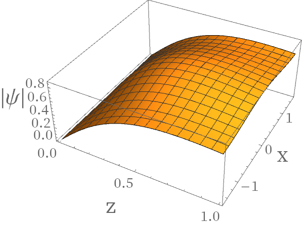
(a) amplitude of $\psi,k=0$

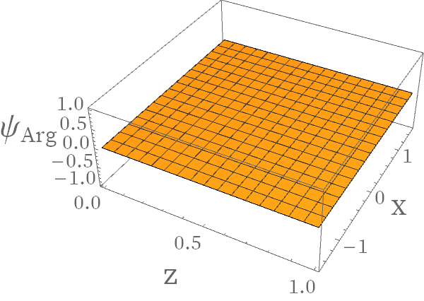
(b) angle of $\psi,k=0$

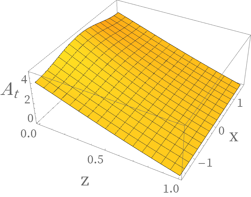
(c) $A_{t},k=0$

(d) amplitude of $\psi,k=0.75$

(e) angle of $\psi,k=0.75$

(f) $A_{t},k=0.75$

Figure 1: The amplitude and phase angle of the bulk field $\psi$ are plotted in subfigures 1(a), 1(b), 1(d) and 1(e); The bulk field $A_{t}$ is plotted in subfigures 1(c) and 1(f). All the fields are calculated at $k=0$ and $0.75$.

(a) Lowest Bloch band $\mu({k})$

(b) Critical optical lattice strength $v_{c}$

Figure 2: Fig. 2(a) shows the lowest Bloch band $\mu(k)$ as a function of Bloch wave vector $k$ with fixed total particle number $N$, whose value is given by the case of chemical potential $\mu=4.5$, lattice strength $v=0.5$ (blue), 4 (red) and Bloch wave vector $k=0$. Fig. 2(b) shows the relation between critical optical lattice strength $v_{c}$ and chemical potential $\mu$. The Bloch band will have loop structure when $v<v_{c}$.

III Bloch waves and Bloch band in optical lattice

From the Bloch theorem and with the source $\Psi_{+}$ turning off, we can use Bloch waves to describe the static response

$$\Psi_{-}\left(z,x\right)=\psi_{B}\left(z,x\right)e^{ikx}.$$ (18)

Here, $\psi_{B}\left(z,x\right)$ is the Bloch wave along the $x$ direction, which has the same period as the optical lattice, i.e. $\psi_{B}\left(z,x+l\right)=\psi_{B}\left(z,x\right)$, $k$ is the Bloch wave vector and $l$ the lattice constant (hereafter we choose $l=\pi$). Due to the fact that Bloch waves are complex functions, we can separate them into real and imaginary parts:

$$\Psi\left(z,x\right)=z\left[\psi_{R}\left(z,x\right)+i\psi_{I}\left(z,x\right)\right]e^{ikx}.$$ (19)

Substituting the above equation into the static equations of motion (10)-(13), we get the following five differential equations:

$$\partial_{z}f\partial_{z}A_{x}+f\partial_{z}^{2}A_{x}=-2\left(\left(\psi_{R}\partial_{x}\psi_{I}-\psi_{I}\partial_{x}\psi_{R}\right)+\left(k-A_{x}\right)\left(\psi_{R}^{2}+\psi_{I}^{2}\right)\right),$$ (20)

$$\partial_{x}\partial_{z}A_{x}=2\left(\psi_{R}\partial_{z}\psi_{I}-\psi_{I}\partial_{z}\psi_{R}\right),$$ (21)

$$f\partial_{z}^{2}A_{t}+\partial_{x}^{2}A_{t}=2A_{t}\left(\psi_{R}^{2}+\psi_{I}^{2}\right),$$ (22)

$$\left(\frac{1}{f}A_{t}^{2}-z-\left(A_{x}-k\right)^{2}\right)\psi_{R}+\partial_{z}\left(f\partial_{z}\psi_{R}\right)+\left(\partial_{x}^{2}\psi_{R}-2\left(k-A_{x}\right)\partial_{x}\psi_{I}+\psi_{I}\partial_{x}A_{x}\right)=0,$$ (23)

$$\left(\frac{1}{f}A_{t}^{2}-z-\left(A_{x}-k\right)^{2}\right)\psi_{I}+\partial_{z}\left(f\partial_{z}\psi_{I}\right)+\left(\partial_{x}^{2}\psi_{I}+2\left(k-A_{x}\right)\partial_{x}\psi_{R}-\psi_{R}\partial_{x}A_{x}\right)=0.$$ (24)

Among them, Eq.(21) will be satisfied automatically if the other four equations are solved. To obtain the static or steady-flow states of the superfluid, we impose the source free boundary conditions for $\Psi_{+}$ and $A_{x}$ at the conformal boundary, regular conditions for $\Psi_{-}$ and $A_{t}=0$ at the horizon and periodic boundary conditions for $A_{t,x}$ and $\Psi$ in the $x$ direction. And the optical lattice structure is imposed by choosing $V(x)=v\cos(2x)$, i.e. $\left.A_{t}\right|_{z=0}=4.5+v\cos(2x)$, with $v$ the height (or strength) of the optical lattice. We solve these four static equations of motion (20), (22), (23) and (24) numerically with the Newton-Raphson method.

Fig.1 shows the numerical solutions of the bulk fields $\psi$ and $A_{t}$, respectively, with two different Bloch wave vectors. Since $\psi$ is complex, we plot its amplitude and phase angle separately. The inexistence of node of order parameter means that these Bloch waves sit in the lowest Bloch band. In Fig. 2(a), we plot the Bloch band in our holographic model. To obtain it, we fix the total particle number, defined as

$$N\equiv\int_{-\frac{\pi}{2}}^{\frac{\pi}{2}}dx\rho,$$ (25)

and solve the static equations (20) and (22)-(24) with $k$ given different values. The loop structure of the blue line ($v=0.5$), at which comes from particle interaction energy is larger than the optical lattice strength PhysRevA.86.063636 , is witnessed around the edge $k=1$ of the Brillouin zone. And for the red line ($v=4$) there is no loop structure. Here, the Bloch band also confirms that the static solution in Fig. 1 are Bloch wave solutions. Actually, the higher value of chemical potential $\mu$, the larger density of total particle $\rho$ in one lattice and hence the larger value of particle interaction energy, which means that when we increase the chemical potential the critical value of the optical lattice strength $v_{c}$ that exceeds the particle interaction energy to prevent the loop structure from appearing will also increase. And we confirm this in Fig. 2(b).

IV Instability and sound modes

Now we study the linear instability of the Bloch wave solutions obtained in the previous section via QNM analyses. To calculate the QNM, a better choice is to rewrite the static equations of motions (10)-(13) with the Bloch wave form for $\psi$ in the infalling Eddington-Finkelstein coordinates Li:2020ayr :

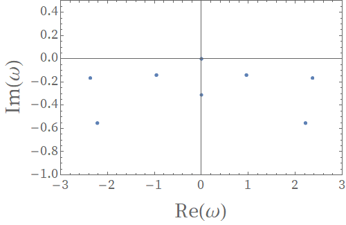
(a) QNM with $k=0,q=0$

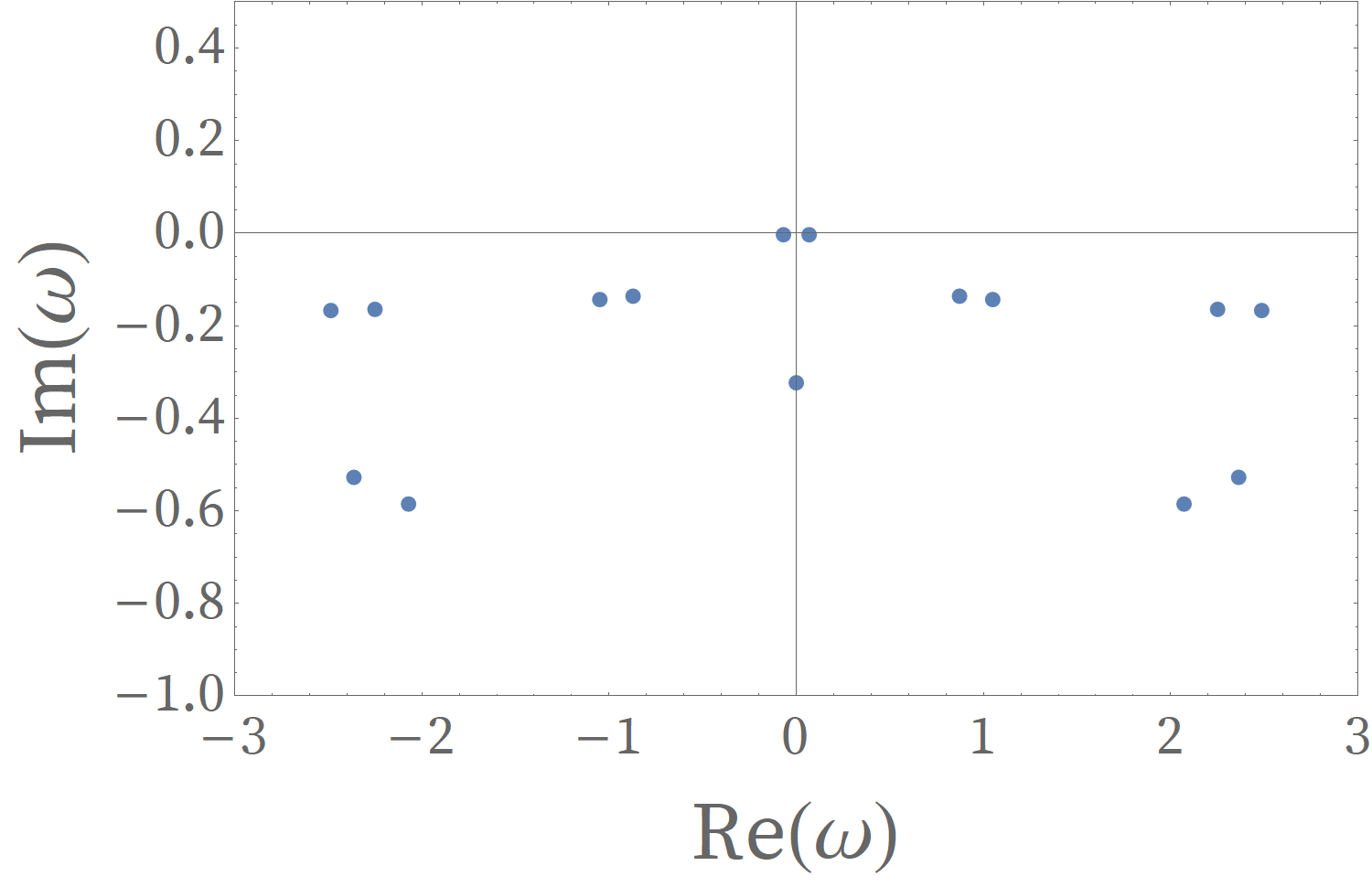
(b) QNM with $k=0,q=0.15$

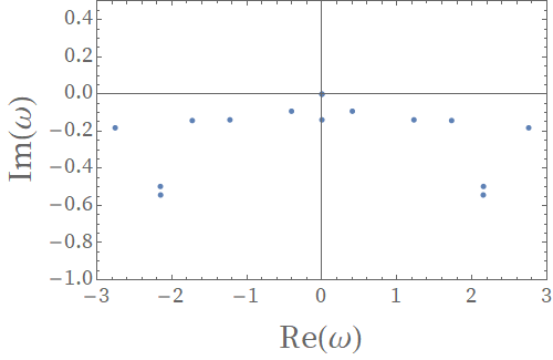
(c) QNM with $k=0.75,q=0$

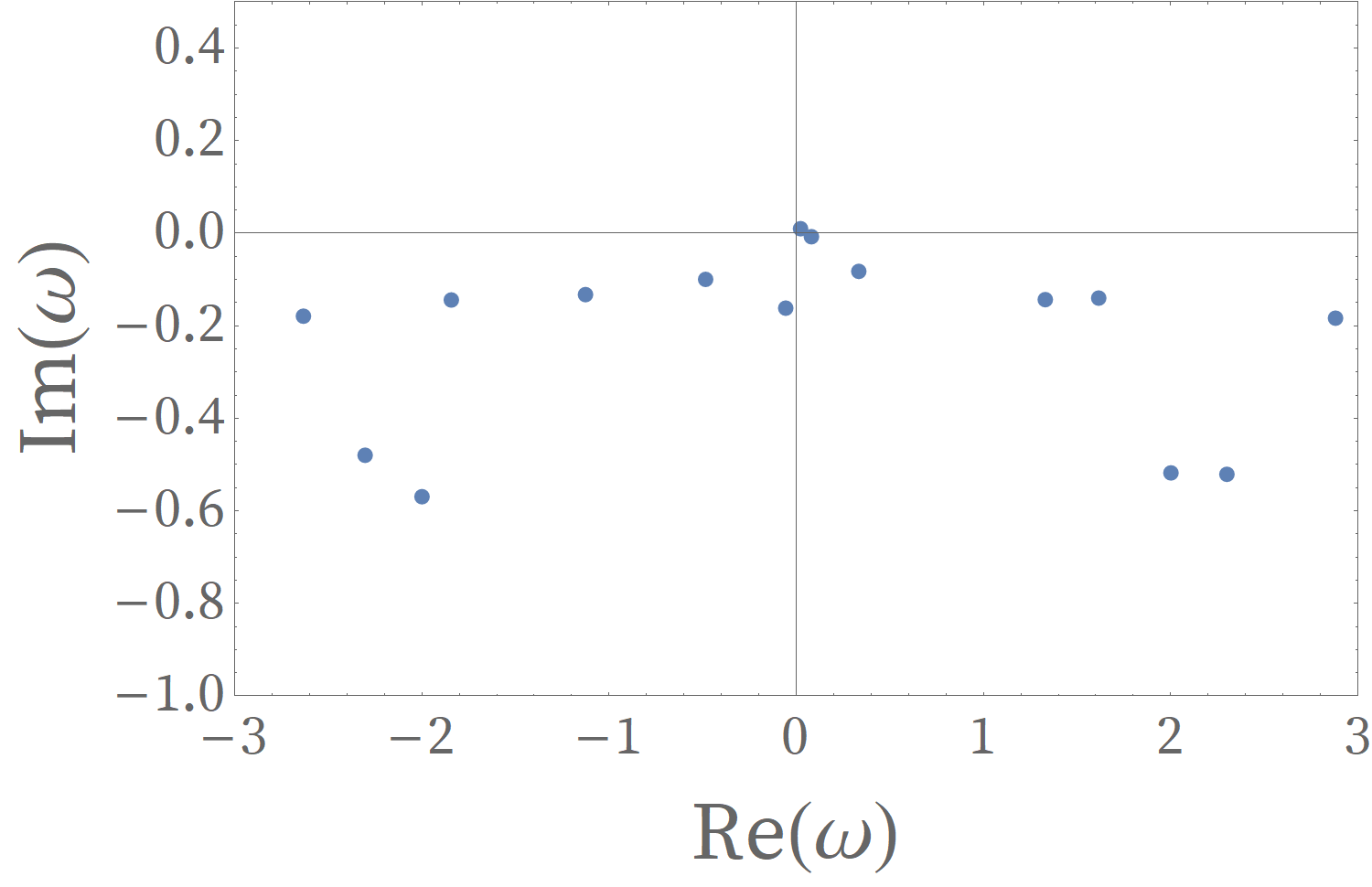
(d) QNM with $k=0.75,q=0.15$

Figure 3: 3(a) and 3(b) show the QNM corresponding to $\psi$’s Bloch wave vector $k=0$ and wave vectors of the perturbed field $q=0$ (left) and $q=0.15$ (right), respectively; 3(c) and 3(d) show the QNM corresponding to $\psi$’s Bloch wave vector $k=0.75$ and wave vectors of the perturbed field $q=0$ (left) and $q=0.15$ (right), respectively. Actually, the QNM is symmetric under Re($\omega$)$\rightarrow-$Re($\omega$) when q=0 and we confirm this in Appendix A.

$$2\partial_{t}\partial_{z}A_{x}-\partial_{z}\partial_{x}A_{t}-\partial_{z}\left(f\partial_{z}A_{x}\right)+i\left(\psi^{*}\partial_{x}\psi-\psi\partial_{x}\psi^{*}-2i\left(A_{x}-k\right)\psi^{*}\psi\right)=0,$$ (26)

$$\begin{split}\partial_{t}\partial_{z}A_{t}+\partial_{t}\partial_{x}A_{x}-\partial_{x}^{2}A_{t}-f\partial_{x}\partial_{z}A_{x}+i\left(\psi^{*}\partial_{t}\psi-\psi\partial_{t}\psi^{*}\right)\\ -if\left(\psi^{*}\partial_{z}\psi-\psi\partial_{z}\psi^{*}\right)+2\psi^{*}A_{t}\psi=0,\end{split}$$ (27)

$$\left(-\partial_{z}^{2}A_{t}+\partial_{x}\partial_{z}A_{x}\right)+i\left(\psi^{*}\partial_{z}\psi-\psi\partial_{z}\psi^{*}\right)=0,$$ (28)

$$\begin{split}2\partial_{t}\partial_{z}\psi-f\partial_{z}^{2}\psi-\left(f^{\prime}+2iA_{t}\right)\partial_{z}\psi-\partial_{x}^{2}\psi+2i\left(A_{x}-k\right)\partial_{x}\psi\\ +\left(-i\partial_{z}A_{t}+i\partial_{x}A_{x}+z+\left(A_{x}-k\right)^{2}\right)\psi=0,\end{split}$$ (29)

where the metric is

$$ds^{2}=\frac{1}{z^{2}}\left(-f(z)dt^{2}-dtdz+dx^{2}+dy^{2}\right).$$

Here and in the following sections we will not separate $\psi$ into real and imaginary parts. Similarly, there is one constraint equation, which is chosen to be Eq.(27). Next, we give all the bulk field perturbations

$$\delta A_{t} =e^{-i\omega t+iqx}a+e^{i\omega^{*}t-iqx}a^{*},$$ (30)

$$\delta A_{x} =e^{-i\omega t+iqx}b+e^{i\omega^{*}t-iqx}b^{*},$$

$$\delta\psi =e^{-i\omega t+iqx}u+e^{i\omega^{*}t-iqx}v^{*}.$$

Substitute these perturbed fields into the equations of motion, we will get the linear perturbation equations

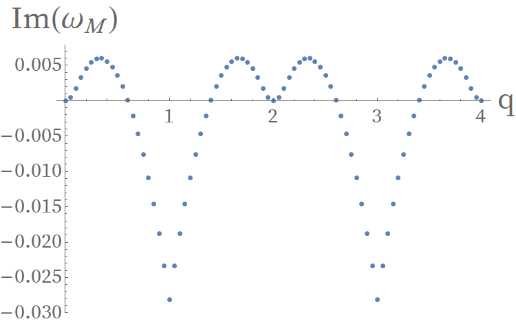
(a) $k=0.7,q\in[0,4]$

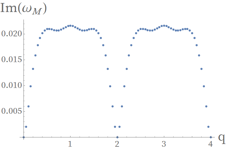
(b) $k=0.75,q\in[0,4]$

Figure 4: $\operatorname{Im}(\omega_{M})$ as a function of $q$ when Bloch wave vector $k=0.7,0.75$.

$$\begin{array}[]{c}\partial_{z}\left(\partial_{x}b+iqb\right)+\left(iv\partial_{z}\psi+i\psi^{*}\partial_{z}u\right)-\left(iu\partial_{z}\psi^{*}+i\psi\partial_{z}v\right)-\partial_{z}^{2}a=0,\end{array}$$ (31)

$$\begin{array}[]{c}\left(2b\psi\psi^{*}+2\left(A_{x}-k-\frac{1}{2}q\right)\psi^{*}u+2\left(A_{x}-k+\frac{1}{2}q\right)\psi v\right)-2i\omega\partial_{z}b+\\ i\left(v\partial_{x}\psi+\psi^{*}\partial_{x}u\right)-i\left(u\partial_{x}\psi^{*}+\psi\partial_{x}v\right)-\partial_{z}\left(f\partial_{z}b\right)-\partial_{z}\left(\partial_{x}a+iqa\right)=0,\end{array}$$ (32)

$$\begin{array}[]{c}\left(z+\left(A_{x}-k-q\right)^{2}+i\left(\partial_{x}A_{x}-\partial_{z}A_{t}\right)\right)u+\left(2\left(A_{x}-k\right)b+i\left(\partial_{x}b+iqb-\partial_{z}a\right)\right)\psi-\\ \left(2i\omega+f^{\prime}+2iA_{t}\right)\partial_{z}u+2i\left(A_{x}-k-q\right)\partial_{x}u-f\partial_{z}^{2}u-\partial_{x}^{2}u-2ia\partial_{z}\psi+2ib\partial_{x}\psi=0,\end{array}$$ (33)

$$\begin{array}[]{c}\left(z+\left(A_{x}-k+q\right)^{2}-i\left(\partial_{x}A_{x}-\partial_{z}A_{t}\right)\right)v+\left(2\left(A_{x}-k\right)b-i\left(\partial_{x}b+iqb-\partial_{z}a\right)\right)\psi^{*}-\\ \left(2i\omega+f^{\prime}-2iA_{t}\right)\partial_{z}v-2i\left(A_{x}-k+q\right)\partial_{x}v-f\partial_{z}^{2}v-\partial_{x}^{2}v+2ia\partial_{z}\psi^{*}-2ib\partial_{x}\psi^{*}=0.\end{array}$$ (34)

In accordance with the background steady solutions, we impose Dirichlet and periodic boundary conditions for $a$, $b$, $u$ and $v$ at $z=0$ and in the $x$ direction, respectively, while regular boundary conditions are chosen at the horizon $z=1$. Then, we can obtain $\omega$ from the perturbation equations by solving generalized eigenvalue problems if $k$ and $q$ are given. (See Appendix A for more details about this procedure.)

The perturbations in Eq.(30) will grow exponentially in the linear regime if there exists an $\omega$ whose imaginary part is positive. We use $\omega_{M}$ to denote the $\omega$ with the maximal imaginary part when $q$ and $\mu$ are given, so a system is (linearly) unstable if $\operatorname{Im}(\omega_{M})>0$. Fig. 3 shows the result for the distributions of $\omega$ with two different values for Bloch wave vector $k$ and $q$. In Fig. 3(a) and Fig. 3(b), $\operatorname{Im}(\omega_{M})\leq 0$, so the $k=0$ solution is stable under perturbations $q=0$ and $q=0.15$. By comparison, the solution at $k=0.75$ is unstable because $\operatorname{Im}(\omega_{M})>0$ in Fig. 3(d), despite the fact that in Fig. 3(c) $\operatorname{Im}(\omega_{M})\leq 0$. A system is stable only when $\operatorname{Im}(\omega_{M})\leq 0$ for all values of $q$.

Actually we find that there are two special values $k_{c}$ and $q_{M}$ for the Bloch waves. $k_{c}$ means the critical wave vector exceeding which the Bloch wave vector $k$ will lead to an unstable state; $q_{M}$ means the Bloch wave vector of the most unstable perturbation mode, which has a maximal imaginary value of $\omega_{M}$, since it will increase with time $t$ with the form $e^{\omega_{I}t}$ controlled by the linear perturbation equations in early times (the late time behavior will be more interesting and it will be investigated in the next section.). Fig. 4 shows the value of $\omega_{M}$ with respect to $q\in[0,4]$, the periodicity and $q_{M}$ can be seen directly.

As we have explained, when $q$ and $k$ are given, $\omega_{M}$ can be obtained to determine the stability under the corresponding perturbation. In this spirit, we plot stable and unstable regions as a function of $q$ and $k$, i.e. the instability diagram, in the half first Brillouin zone in Fig. 5. In this plot, the left region in the figure, which is colored darker grey, is stable ($\operatorname{Im}(\omega_{M})\leq 0$), and the right region in the figure, which is colored lighter grey, is unstable ($\operatorname{Im}(\omega_{M})>0$). The figure also tells us that in the unstable region the cutoff $q$ increases with $k$, and when $k$ is large enough (but still in the first Brillouin zone), the system is unstable for all values of $q$ except $q=0$.

Figure 5: Instability diagram for Bloch waves with $k\in[0,1]$ and $q\in[0,1]$. In the darker grey region (the left part in the figure), $\operatorname{Im}(\omega_{M})\leq 0$, and in the lighter grey region (the right part in the figure), $\operatorname{Im}(\omega_{M})>0$.

As a signal of onset of the instability mentioned in 2014JHEP…02..063A ; 2020arXiv201006232L , we also plot the dispersion relation of the sound mode in Fig.6. When there is a non-zero $k$ the sound speed becomes direction-dependent. There are two directions corresponding to the maximal and minimal values of the sound speed, which are parallel ($q>0$) and anti-parallel ($q<0$) to the velocity of the superflow, respectively. Hereafter we denote the sound speed as $c_{+}$ for $q>0$ and $c_{-}$ for $q<0$.

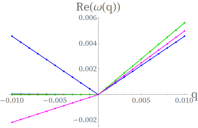
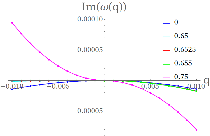
Figure 6: Dispersion relations for sound modes at $k=0,0.65,0.6525,0.655,0.75$. Left panel shows $\operatorname{Re}(\omega(q))$ and right panel shows $\operatorname{Im}(\omega(q))$. A universal phenomenon is that $\operatorname{Im}(\omega(q))>0$ always accompanies $\operatorname{Re}(\omega(q))<0$.

The onset of instability is accompanied by the sign-change of $c_{-}$. Along the negative axis of $q$, $\operatorname{Re}(\omega)$ becomes negative as $k$ is larger than 0.655. As $\operatorname{Re}(\omega)$ corresponds to the energy of the perturbation, $c_{-}<0$ (so $\operatorname{Re}(\omega)<0$) indicates the existence of a perturbed state with lower energy and thus the instability of the system (Landau instability). At the same time, we find that $\operatorname{Im}(\omega)>0$, which implies the dynamical instability of the system. So, our result confirms that the Landau instability and dynamical instability occur at the same time, as we have mentioned.

For the purpose of opening the next section we give a brief discussion about this section. Since it is not always true for a superflow to flow in the optical lattice stably, when $k\geq k_{c}$ excitations will always appear to slow the superflow down 2020arXiv201006232L , but what kind of intermediate states will this unstable superflow go through and what kind of final states will it end up with? In the next section we will use full nonlinear evolution to find the final state out for the Bloch wave-type superflow and the intermediate states will also be discussed.

V Real time evolution for stable and unstable superflows

To simulate the evolution of the holographic superfluid, we adopt the same scheme as in Li:2020ayr , i.e. taking Eqs.(26), (28) and (29) as evolution equations while choosing Eq.(27) as the constraint. Since Eq.(28) does not have time derivative terms but have space derivatives up to the second order, it can be solved with one boundary condition from $A_{t}(z_{b})=4.5+0.5\cos(2x)$ and another from the restriction of Eq.(27) on the conformal boundary. In the spatial directions the pseudo-spectral method is chosen for discretization, while in the time direction we adopt the fourth order Runge-Kutta method. When doing the time evolution, we choose static solutions, including $\psi$, $A_{t}$ and $A_{x}$ which are solved from the static equations of motion, as the initial states (at $t=0$), and at an early time $t_{1}$ we add perturbations, which are some random functions with small amplitudes, to $\psi$. Here, we require that the perturbations should not break the source free boundary condition of $\psi$. The perturbation is not necessarily periodic and there are many lattice cells in experiments, so it is necessary to include more lattice cells into the time evolution.

V.1 Evolution of particle current density

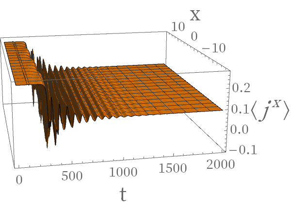
(a) $\langle j^{x}(t,x)\rangle$

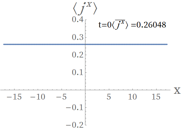
(b) $t=0$

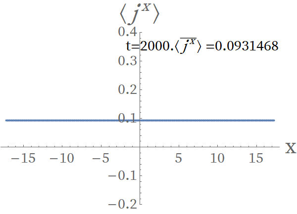
(c) $t=2000$

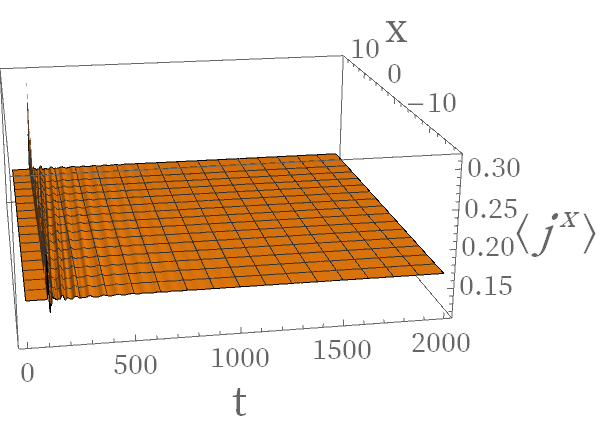
(d) $\langle j^{x}(t,x)\rangle$

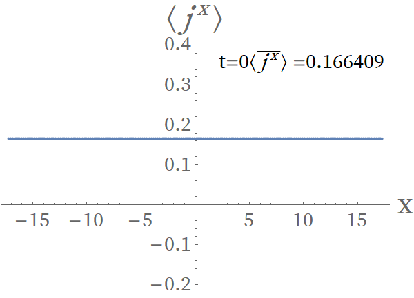
(e) $t=0$

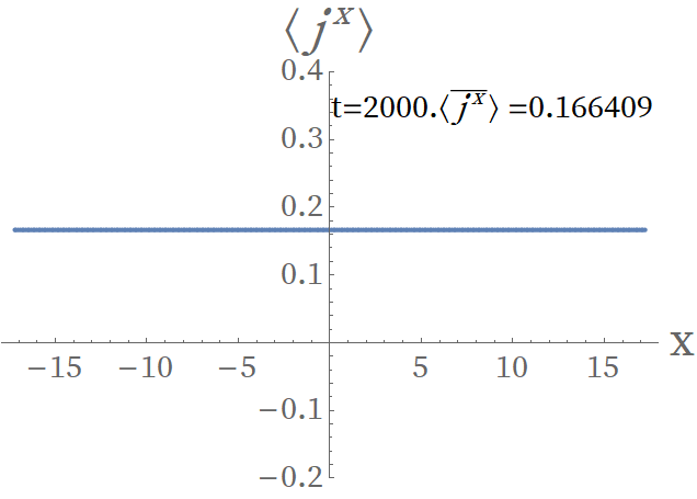
(f) $t=2000$

Figure 7: Evolutions for superflows with $k=0.3$ (stable) and $k=0.75$ (unstable), respectively. These panels show the particle current density with $t\in[0,2000]$.

We introduce perturbations at $t=100$, i.e. $t_{1}=100$, and observe the evolution of the systems with initial Bloch vectors $k$ chosen as $0.3$ and $0.75$, respectively. Fig. 7 shows the evolution of the particle current density $\langle j^{x}\rangle$, which is defined as

$$\langle j^{x}\rangle=\lim_{z\to 0}\sqrt{-g}F^{zx}.$$ (35)

From Fig. 7, the evolution of $\langle j^{x}\rangle$ of an unstable superflow can be divided into five stages. In the first stage $t<100$, no change is observed, which confirms that the static solutions obtained in the Schwarzschild coordinates is correctly transformed to that in the Eddington-Finkelstein coordinates. When $100<t<200$, the current density changes slightly since the influence of the perturbation is small; when $200<t<400$, the current density becomes chaotic, which comes from the nonlinear development of the instability. When $400<t<1500$, the chaotic behavior of the current density disappears but the current is still inhomogeneous; In this stage, the system is tending to a steady state. In the last stage $t>1500$, the system becomes steady with the final current density $\langle j^{x}\rangle_{f}=0.0931468$, which is much smaller than the initial value 0.26048. In contrast, for the stable superflow ($k=0.3$ as an example for comparison) the situation is totally different. The influence of perturbations on the system is insignificant and the system will evolve to a state that is same as the initial state in a few moments.

V.2 Evolution of condensate and intermediate states

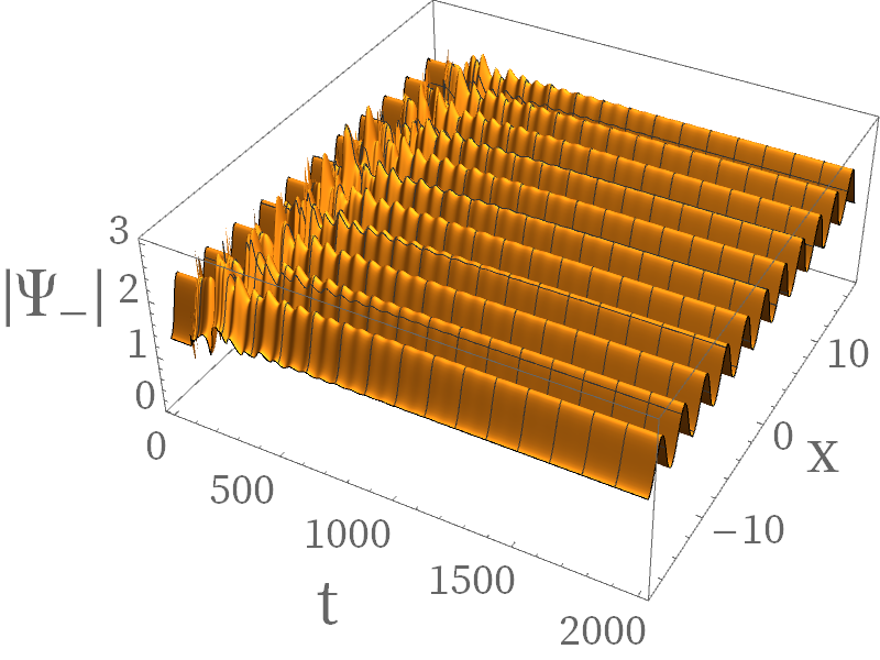
(a) $|\Psi_{-}|(t,x)$

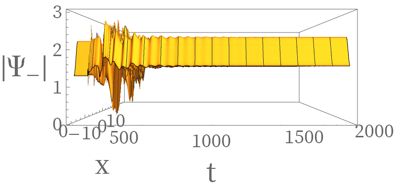
(b) $|\Psi_{-}|(t,x)$

(c) $|\Psi_{-}|(t,x)$

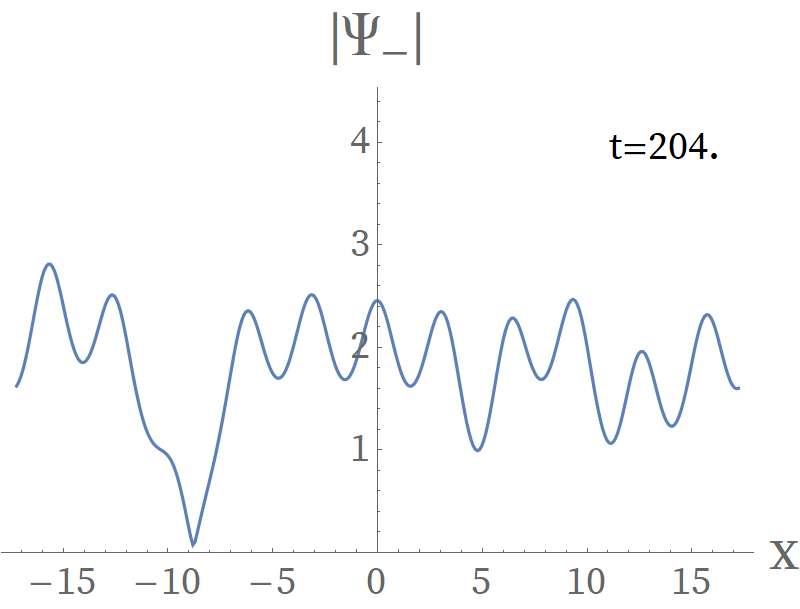
(d) $t=204$

Figure 8: Evolution of the condensate $|\Psi_{-}(t,x)|$ with $t\in[0,2000]$ of the unstable superflow $k=0.75$. The perturbation is given at $t=100$; After that there are some solitons generated, as plotted in Fig. 8(d).

As we have seen from the evolution of $\langle j^{x}\rangle$, the intermediate states of the system are chaotic and complicated. However, there are some universal features which can be extracted from the evolution of the condensate $|\Psi_{-}|$ and we plot them in Fig. 8.

We plot the evolution of $|\Psi_{-}|$ from different viewing angles, i.e. Fig. 8(a), Fig. 8(b) and Fig. 8(c). Fig. 8(a) is from an ordinary viewing angle, from which we can see the complete picture of $|\Psi_{-}(t,x)|$; Fig. 8(b) is plotted with the viewing angle along the $x$ axis. We can see that the condensate during $100<t<400$ is also chaotic and the value of $|\Psi_{-}|$ at later times is larger than its initial value. The planform of $|\Psi_{-}|$ is plotted at Fig. 8(c) and nodes of the order parameter appear during $100<t<400$, which indicates the formation of solitons. We select one moment ($t=204$) of the soliton formation in Fig. 8(d). The formation of solitons is natural here 2020arXiv201006232L since the unstable superflow is thought of as having a higher free energy than a less unstable superflow with soliton excitations. Along with the dissipative processes, the whole system will go to a stable state with a lower free energy.

V.3 Final stable state

Since both $\langle j^{x}\rangle$ and $|\Psi_{-}|$ become time independent at the end of the evolution, the final state of the system must be able to be described as a Bloch state just like the initial steady flow states that are solved in Sec. III. This is indeed the case. Actually, the final state can also be solved from the equations of motion, i.e. (20), (22), (23) and (24), with an additional boundary condition besides the boundary conditions given in Sec. III, while not specifying the Bloch wave vector $k$.

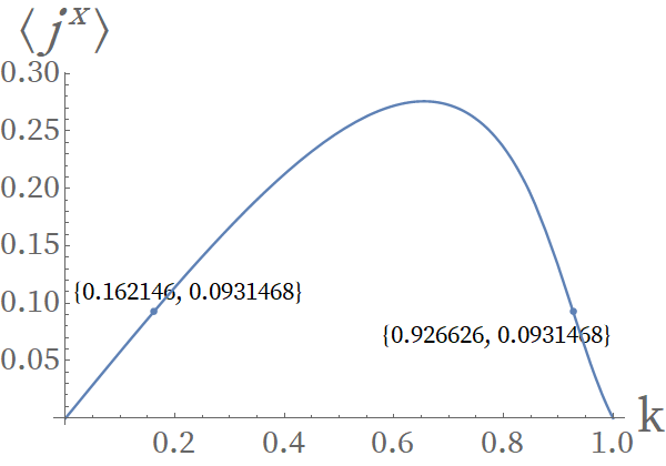
(a) $\langle j^{x}(k)\rangle$

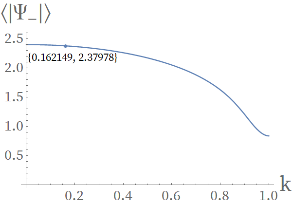
(b) $\langle|\Psi_{-}|(k)\rangle$

Figure 9: Relations between $\langle j^{x}\rangle$ and $k$ as well as $\langle|\Psi_{-}|\rangle$ and $k$. Both figures are obtained by interpolation with discrete value of k, so the value 0.162146, 0.926626 and 2.37978 is not exact. The non-monotonicity for $\langle j^{x}\rangle$ gives two states with different $k$, while the monotonicity for $\langle|\Psi_{-}|\rangle$ excludes the larger $k$ state.

When there is a one-to-one correspondence between $\langle j^{x}\rangle$ and the Bloch wave vector $k$, one can get the additional boundary condition directly by fixing $\langle j^{x}\rangle=\langle j^{x}\rangle_{f}$. However, as we can find from Fig. 9(a), i.e. the relation between $\langle j^{x}\rangle$ and $k$, a fixed $\langle j^{x}\rangle$ normally corresponds to two values of $k$. To make the solution unique, we can take account of the average condensate $\langle|\Psi_{-}|\rangle$ in one lattice cell. From Fig. 8(a) we know that the condensate amplitude $|\Psi_{-}|$ of a steady state is not a constant, so the relation between $|\Psi_{-}|$ and $k$ is not clear, while $\langle|\Psi_{-}|\rangle$ is a monotonically decreasing function of $k$, as plotted in Fig. 9(b). Therefore, the boundary condition can be uniquely determined by combining the two considerations: $\langle j^{x}\rangle=\langle j^{x}\rangle_{f}$ and the value of $\langle|\Psi_{-}|\rangle$. From Fig. 8(b) and Fig. 7(c) we conclude that the final Bloch state corresponds to a larger $\langle|\Psi_{-}|\rangle$ with $\langle j^{x}\rangle=0.0931468$, thus we can solve the equations of motion with the additional boundary condition $\partial_{z}{A_{x}}|_{z=0}=0.0931468$, and the solution is marked on Fig. 9(b).

VI Summary

The dynamical process of superfluids that simultaneously experiences Landau and dynamical instability in optical lattice is investigated using the simplest holographic superfluid model. Due to the existence of dissipation the sound mode of an unstable superflow will always have negative energy and grows up exponentially at early times. We give a universal picture of the instability process for the unstable superflow. From real time evolution the unstable superflow is shown to reduce its particle current density to settle down to a steady state with a current density $\langle j^{x}\rangle_{f}$ and a Bloch wave vector $k_{f}$ below the critical value $k_{c}$, where this $k_{f}$ can be solved from the equations of motion by fixing $\langle j^{x}\rangle=\langle j^{x}\rangle_{f}$. In the course of the evolution, a chaotic process involving soliton generation is observed, in which the solitons are supposed to play the role of reducing the wave vector $k$ (similar to the case without an optical lattice 2020arXiv201006232L ).

As we have mentioned, when the number of dimensions of the boundary system is greater than one, the process for an unstable state to evolve into a stable one will become much more complicated, which to some extent is described as transient turbulence 2020arXiv201006232L . So beside the one dimensional boundary superfluid system in optical lattice, it is worthwhile to consider higher dimensional cases. Another direction for future investigation is to include backreaction in this holographic superfluid model, which will enable us to explore the complete interplay between the normal fluid and superfluid components of the superflow at a finite temperature in optical lattice.

Appendix A Notes on generalized eigenvalue problems

Let’s begin at the bulk fields perturbation (30). It’s well known that when a system has the symmetry of time translation, then any field $F(t,x)$ can be separated into mode $f(x)e^{-i\omega t}$ with different $\omega$. The situation is similar for space. If there is a continuous space translation symmetry, then we have $F(t,x)\sim f(t)e^{ikx}$ with continuous value of $k$; if there is a discrete space translation symmetry, then we also have $F(t,x)\sim f(t)e^{ikx}$ but with discrete value of $k=\frac{2\pi}{L}n$, where $n$ is integer and $L$ is lattice constant.

But in our case, we do not use the above separation though there is a discrete space translation symmetry but use Bloch wave to describe the $x$ direction of the fields, i.e. $F(t,x)=f(t,x)e^{iqx}$. Here F(t,x) and f(t,x) can be complex functions and we can do some deformations,

$$\begin{split}F(t,x)&=f(t,x)e^{iqx}\\ &=\frac{1}{2}(f(t,x)e^{iqx}+f^{*}(t,x)e^{-iqx})+\frac{1}{2}(f(t,x)e^{iqx}-f^{*}(t,x)e^{-iqx})\\ &=\frac{1}{2}(f(t,x)+f^{*}(t,x)e^{-2iqx})e^{iqx}+\frac{1}{2}(f(t,x)e^{2iqx}-f^{*}(t,x))e^{-iqx}\\ &=g(t,x)e^{iqx}+h(t,x)^{*}e^{-iqx}.\end{split}$$ (36)

With this deformation we can write (30) and get (31)-(34) straightforward.

Equations (31)-(34) can be written as a matrix form, i.e.,

$$R\left(\begin{array}[]{l}a\\ b\\ u\\ v\end{array}\right)=\omega A\left(\begin{array}[]{l}a\\ b\\ u\\ v\end{array}\right),$$ (37)

with appropriate boundary conditions given in Section IV. These function is indeed the general eigenvalue function and there are many methods in textbook to solve this function to get the eigenvalue $\omega$.

Before we calculate the value of $\omega$ we can know that if $\omega_{R}$ is real part of one of the eigenvalue $\omega$, then there must be another value of $\omega$ whose real part equals to -$\omega_{R}$. To show this we can define a matrix $L$, which is defined as

$$L=R-\omega A,$$ (38)

then Eq.(37) can be written as

$$L\left(\begin{array}[]{l}a\\ b\\ u\\ v\end{array}\right)=0.$$ (39)

Separate $\omega$ into real part and imaginary pary and we get that the imaginary part of $L$ only contains $\omega_{R}$, which means

$$L_{I}(\omega_{R})\left(\begin{array}[]{l}a\\ b\\ u\\ v\end{array}\right)=0.$$ (40)

From Equations (31)-(34) it is easy to get that when $q=0$ the following relation exists, i.e.,

$$L_{I}(\omega_{R})\left(\begin{array}[]{l}a\\ b\\ u\\ v\end{array}\right)=-L_{I}(-\omega_{R})\left(\begin{array}[]{l}a\\ b\\ v\\ u\end{array}\right).$$ (41)

Since the boundary conditions for $u$ and $v$ are the same, changing the places between $u$ and $v$ do not affect the eigenvalues. While when $q\neq 0$, there do not have the relation (41).

References

- [1] Biao Wu and Qian Niu. Landau and dynamical instabilities of the superflow of bose-einstein condensates in optical lattices. Phys. Rev. A, 64:061603, Nov 2001.
- [2] Biao Wu and Qian Niu. Superfluidity of bose–einstein condensate in an optical lattice: Landau–zener tunnelling and dynamical instability. New Journal of Physics, 5:104–104, jul 2003.
- [3] Qian Niu, Xian-Geng Zhao, G. A. Georgakis, and M. G. Raizen. Atomic Landau-Zener Tunneling and Wannier-Stark Ladders in Optical Potentials. Phys. Rev. L, 76(24):4504–4507, June 1996.
- [4] Biao Wu and Qian Niu. Nonlinear Landau-Zener tunneling. Phys. Rev. A, 61(2):023402, February 2000.
- [5] M. Cristiani, O. Morsch, J. H. Müller, D. Ciampini, and E. Arimondo. Experimental properties of Bose-Einstein condensates in one-dimensional optical lattices: Bloch oscillations, Landau-Zener tunneling, and mean-field effects. Phys. Rev. A, 65(6):063612, June 2002.
- [6] M. Jona-Lasinio, O. Morsch, M. Cristiani, N. Malossi, J. H. Müller, E. Courtade, M. Anderlini, and E. Arimondo. Asymmetric Landau-Zener Tunneling in a Periodic Potential. Phys. Rev. L, 91(23):230406, December 2003.
- [7] Q. Guan, M. K. H. Ome, T. M. Bersano, S. Mossman, P. Engels, and D. Blume. Nonexponential Tunneling due to Mean-Field-Induced Swallowtails. Phys. Rev. L, 125(21):213401, November 2020.
- [8] D. Jaksch, C. Bruder, J. I. Cirac, C. W. Gardiner, and P. Zoller. Cold Bosonic Atoms in Optical Lattices. Phys. Rev. L, 81(15):3108–3111, October 1998.
- [9] V. A. Kashurnikov, N. V. Prokof’ev, and B. V. Svistunov. Revealing the superfluid-Mott-insulator transition in an optical lattice. Phys. Rev. A, 66(3):031601, September 2002.
- [10] A. Smerzi, A. Trombettoni, P. G. Kevrekidis, and A. R. Bishop. Dynamical Superfluid-Insulator Transition in a Chain of Weakly Coupled Bose-Einstein Condensates. Phys. Rev. L, 89(17):170402, October 2002.
- [11] S. R. Clark and D. Jaksch. Dynamics of the superfluid to Mott-insulator transition in one dimension. Phys. Rev. A, 70(4):043612, October 2004.
- [12] Jakub Zakrzewski. Mean-field dynamics of the superfluid-insulator phase transition in a gas of ultracold atoms. Phys. Rev. A, 71(4):043601, April 2005.
- [13] Esteban Calzetta, B. L. Hu, and Ana Maria Rey. Bose-Einstein-condensate superfluid-Mott-insulator transition in an optical lattice. Phys. Rev. A, 73(2):023610, February 2006.
- [14] Marin Bukov, Luca D’Alessio, and Anatoli Polkovnikov. Universal high-frequency behavior of periodically driven systems: from dynamical stabilization to Floquet engineering. Advances in Physics, 64(2):139–226, March 2015.
- [15] Marin Bukov, Sarang Gopalakrishnan, Michael Knap, and Eugene Demler. Prethermal floquet steady states and instabilities in the periodically driven, weakly interacting bose-hubbard model. Phys. Rev. Lett., 115:205301, Nov 2015.
- [16] Michael Messer, Kilian Sandholzer, Frederik Görg, Joaquín Minguzzi, Rémi Desbuquois, and Tilman Esslinger. Floquet dynamics in driven fermi-hubbard systems. Phys. Rev. Lett., 121:233603, Dec 2018.
- [17] T. Boulier, J. Maslek, M. Bukov, C. Bracamontes, E. Magnan, S. Lellouch, E. Demler, N. Goldman, and J. V. Porto. Parametric heating in a 2d periodically driven bosonic system: Beyond the weakly interacting regime. Phys. Rev. X, 9:011047, Mar 2019.
- [18] Christian Schweizer, Fabian Grusdt, Moritz Berngruber, Luca Barbiero, Eugene Demler, Nathan Goldman, Immanuel Bloch, and Monika Aidelsburger. Floquet approach to lattice gauge theories with ultracold atoms in optical lattices. Nature Physics, 15(11):1168–1173, September 2019.
- [19] J. C. Bronski, L. D. Carr, R. Carretero-González, B. Deconinck, J. N. Kutz, and K. Promislow. Stability of attractive Bose-Einstein condensates in a periodic potential. Phys. Rev. E, 64(5):056615, November 2001.
- [20] J. C. Bronski, L. D. Carr, B. Deconinck, J. N. Kutz, and K. Promislow. Stability of repulsive Bose-Einstein condensates in a periodic potential. Phys. Rev. E, 63(3):036612, March 2001.
- [21] F. S. Cataliotti, L. Fallani, F. Ferlaino, C. Fort, P. Maddaloni, and M. Inguscio. Superfluid current disruption in a chain of weakly coupled Bose Einstein condensates. New Journal of Physics, 5(1):71, June 2003.
- [22] L. Fallani, L. de Sarlo, J. E. Lye, M. Modugno, R. Saers, C. Fort, and M. Inguscio. Observation of Dynamical Instability for a Bose-Einstein Condensate in a Moving 1D Optical Lattice. Phys. Rev. L, 93(14):140406, September 2004.
- [23] M. Modugno, C. Tozzo, and F. Dalfovo. Role of transverse excitations in the instability of Bose-Einstein condensates moving in optical lattices. Phys. Rev. A, 70(4):043625, October 2004.
- [24] Wenxian Zhang, D. L. Zhou, M.-S. Chang, M. S. Chapman, and L. You. Dynamical instability and domain formation in a spin-1 bose-einstein condensate. Phys. Rev. Lett., 95:180403, Oct 2005.
- [25] J. Ruostekoski and L. Isella. Dissipative quantum dynamics of bosonic atoms in a shallow 1d optical lattice. Phys. Rev. Lett., 95:110403, Sep 2005.
- [26] Kiyohito Iigaya, Satoru Konabe, Ippei Danshita, and Tetsuro Nikuni. Landau damping: Instability mechanism of superfluid Bose gases moving in optical lattices. Phys. Rev. A, 74(5):053611, November 2006.
- [27] S. Konabe and T. Nikuni. Instability of a superfluid Bose gas induced by a locked thermal gas in an optical lattice. Journal of Physics B Atomic Molecular Physics, 39(10):S101–S108, May 2006.
- [28] Samantha Hooley and Keith A. Benedict. Dynamical instabilities in a two-component Bose-Einstein condensate in a one-dimensional optical lattice. Phys. Rev. A, 75(3):033621, March 2007.
- [29] Ai-Xia Zhang and Ju-Kui Xue. The dynamics and stabilities of bose–einstein condensates in deep optical lattices. Physics Letters A, 372(8):1147–1154, 2008.
- [30] Zhao-Xin Liang and Ban-Bi Hu. Stability Diagrams of a Bose-Einstein Condensate in Excited Bloch Bands. Chinese Physics Letters, 26(1):016701, January 2009.
- [31] Rui Asaoka, Hiroki Tsuchiura, Makoto Yamashita, and Yuta Toga. Density Modulations Associated with the Dynamical Instability in the Bose-Hubbard Model. Journal of the Physical Society of Japan, 83(12):124001, December 2014.
- [32] Rui Asaoka, Hiroki Tsuchiura, Makoto Yamashita, and Yuta Toga. Dynamical instability in the bose-hubbard model. Phys. Rev. A, 93:013628, Jan 2016.
- [33] S. Burger, F. S. Cataliotti, C. Fort, F. Minardi, M. Inguscio, M. L. Chiofalo, and M. P. Tosi. Superfluid and dissipative dynamics of a bose-einstein condensate in a periodic optical potential. Phys. Rev. Lett., 86:4447–4450, May 2001.
- [34] F S Cataliotti, L Fallani, F Ferlaino, C Fort, P Maddaloni, and M Inguscio. Superfluid current disruption in a chain of weakly coupled bose–einstein condensates. New Journal of Physics, 5:71–71, jun 2003.
- [35] L. Fallani, L. De Sarlo, J. E. Lye, M. Modugno, R. Saers, C. Fort, and M. Inguscio. Observation of dynamical instability for a bose-einstein condensate in a moving 1d optical lattice. Phys. Rev. Lett., 93:140406, Sep 2004.
- [36] L. De Sarlo, L. Fallani, J. E. Lye, M. Modugno, R. Saers, C. Fort, and M. Inguscio. Unstable regimes for a bose-einstein condensate in an optical lattice. Phys. Rev. A, 72:013603, Jul 2005.
- [37] S Konabe and T Nikuni. Instability of a superfluid bose gas induced by a locked thermal gas in an optical lattice. Journal of Physics B: Atomic, Molecular and Optical Physics, 39(10):S101–S108, may 2006.
- [38] Z. Rapti, P. G. Kevrekidis, A. Smerzi, and A. R. Bishop. Parametric and modulational instabilities of the discrete nonlinear Schrödinger equation. Journal of Physics B Atomic Molecular Physics, 37(7):S257–S264, April 2004.
- [39] M. Krämer, C. Tozzo, and F. Dalfovo. Parametric excitation of a Bose-Einstein condensate in a one-dimensional optical lattice. Phys. Rev. X, 71(6):061602, June 2005.
- [40] N. Gemelke, E. Sarajlic, Y. Bidel, S. Hong, and S. Chu. Parametric Amplification of Matter Waves in Periodically Translated Optical Lattices. Phys. Rev. L, 95(17):170404, October 2005.
- [41] S. Lellouch, M. Bukov, E. Demler, and N. Goldman. Parametric Instability Rates in Periodically Driven Band Systems. Physical Review X, 7(2):021015, April 2017.
- [42] K. Wintersperger, M. Bukov, J. Näger, S. Lellouch, E. Demler, U. Schneider, I. Bloch, N. Goldman, and M. Aidelsburger. Parametric instabilities of interacting bosons in periodically driven 1d optical lattices. Phys. Rev. X, 10:011030, Feb 2020.
- [43] V. V. Konotop and M. Salerno. Modulational instability in Bose-Einstein condensates in optical lattices. Phys. Rev. A, 65(2):021602, February 2002.
- [44] Z. Rapti, P. G. Kevrekidis, A. Smerzi, and A. R. Bishop. Variational approach to the modulational instability. Phys. Rev. E, 69(1):017601, January 2004.
- [45] V. A. Brazhnyi, V. V. Konotop, and V. Kuzmiak. Nature of the Intrinsic Relation between Bloch-Band Tunneling and Modulational Instability. Phys. Rev. L, 96(15):150402, April 2006.
- [46] Shao-Liang Zhang, Zheng-Wei Zhou, and Biao Wu. Superfluidity and stability of a bose-einstein condensate with periodically modulated interatomic interaction. Phys. Rev. A, 87:013633, Jan 2013.
- [47] E. Wamba, S. Sabari, K. Porsezian, A. Mohamadou, and T. C. Kofané. Dynamical instability of a bose-einstein condensate with higher-order interactions in an optical potential through a variational approach. Phys. Rev. E, 89:052917, May 2014.
- [48] Yi Zheng, Marijan Kos˘trun, and Juha Javanainen. Low-acceleration instability of a bose-einstein condensate in an optical lattice. Phys. Rev. Lett., 93:230401, Nov 2004.
- [49] Sean A. Hartnoll, Christopher P. Herzog, and Gary T. Horowitz. Building a holographic superconductor. Phys. Rev. Lett., 101:031601, Jul 2008.
- [50] Sean A Hartnoll, Christopher P Herzog, and Gary T Horowitz. Holographic superconductors. Journal of High Energy Physics, 2008(12):015–015, dec 2008.
- [51] Allan Adams, Paul M. Chesler, and Hong Liu. Holographic Vortex Liquids and Superfluid Turbulence. Science, 341:368–372, 2013.
- [52] Irene Amado, Daniel Areán, Amadeo Jiménez-Alba, Karl Landsteiner, Luis Melgar, and Ignacio Salazar Landea. Holographic superfluids and the Landau criterion. Journal of High Energy Physics, 2014:63, February 2014.
- [53] Shanquan Lan, Hong Liu, Yu Tian, and Hongbao Zhang. Landau Instability and soliton formations. arXiv e-prints, page arXiv:2010.06232, October 2020.
- [54] Xin Li, Yu Tian, and Hongbao Zhang. Generation of vortices and stabilization of vortex lattices in holographic superfluids. JHEP, 02:104, 2020.
- [55] Yu Tian, Xiao-Ning Wu, and Hongbao Zhang. Free energy, stability, and dissipation in dynamical holography. arXiv, 12 2019.
- [56] Hoi-Yin Hui, Ryan Barnett, J. V. Porto, and S. Das Sarma. Loop-structure stability of a double-well-lattice bose-einstein condensate. Phys. Rev. A, 86:063636, Dec 2012.
- [57] Xin Li, Zhang-Yu Nie, and Yu Tian. Holographic boiling and generalized thermodynamic description beyond local equilibrium. JHEP, 09:063, 2020.