Adversarial Training with Contrastive Learning in NLP

Abstract

For years, adversarial training has been extensively studied in natural language processing (NLP) settings. The main goal is to make models robust so that similar inputs derive in semantically similar outcomes, which is not a trivial problem since there is no objective measure of semantic similarity in language. Previous works use an external pre-trained NLP model to tackle this challenge, introducing an extra training stage with huge memory consumption during training. However, the recent popular approach of contrastive learning in language processing hints a convenient way of obtaining such similarity restrictions. The main advantage of the contrastive learning approach is that it aims for similar data points to be mapped close to each other and further from different ones in the representation space. In this work, we propose adversarial training with contrastive learning (ATCL) to adversarially train a language processing task using the benefits of contrastive learning. The core idea is to make linear perturbations in the embedding space of the input via fast gradient methods (FGM) and train the model to keep the original and perturbed representations close via contrastive learning. In NLP experiments, we applied ATCL to language modeling and neural machine translation tasks. The results show not only an improvement in the quantitative (perplexity and BLEU) scores when compared to the baselines, but ATCL also achieves good qualitative results in the semantic level for both tasks without using a pre-trained model.

1 Introduction

Adversarial training has undoubtedly become one of the trending topics in deep learning research in the last decade, since adversarial examples were proposed (Szegedy et al. 2013; Goodfellow, Shlens, and Szegedy 2014). Adversarial examples can be defined broadly as samples specifically crafted to fool a neural model but not a human observer. There are several straightforward ways to craft adversarial examples in computer vision when the model weights and parameters are accessible for the attacker (white-box attack). Some well-known examples based on gradient information are FGSM (Goodfellow, Shlens, and Szegedy 2014), BIM (Kurakin et al. 2016), MI-FGSM (Dong et al. 2018), JSMA (Papernot et al. 2016), and DeepFool (Moosavi-Dezfooli, Fawzi, and Frossard 2016). All these methods result in a corrupted version of an original image, and they are indistinguishable to human observers. After crafting the adversarial examples with one of these methods, the easiest way to make the model robust is to add them to the training set. This adversarial training has a similar effect as regularization by data augmentation (Goodfellow, Shlens, and Szegedy 2014).

In contrast to the computer vision applications, adversarial examples are not well defined in natural language processing (NLP) settings. For example, character-level targeted attacks such as character swapping, insertion or deletion, are always perceptible to humans, but are still considered a type of adversarial examples (Ebrahimi, Lowd, and Dou 2018). Even though there are many definitions of adversarial examples in the natural language field, some works follow a more general definition, analogous to the computer vision’s: samples specifically crafted to fool the model while preserving the semantic of the original phrase as in Alzantot et al. 2018, Jin et al. 2020, Ren et al. 2019, Morris 2020, and Garg and Ramakrishnan 2020. This is the definition we consider in this work, and so we only focus on performing imperceptible perturbations in the word-level.

Since the text tokens belong to a discrete space, directly applying small perturbations is unfeasible. As an alternative, we can apply them in the embedding space (Cheng et al. 2018; Cheng, Jiang, and Macherey 2019). The main goal is to make the model robust to small variations of the input so that small variations of the input should not result in different outcomes. Prior works introduced a pre-trained NLP model to ensure a strong regularization that makes close representations of the original and perturbed samples (Cheng et al. 2018; Cheng, Jiang, and Macherey 2019). However, the errors of the pre-trained model can cause unstable training, and the desired robustness may not be achieved (Zhang et al. 2020). Furthermore, obtaining good adversarial examples via such methods might be computationally expensive, since we have to run the auxiliary model for each sample that we perturbed.

As an alternative, forcing the representation of similar embeddings (the original and its adversarial perturbation) to be mapped into similar outputs may suggest the usage of contrastive learning. Contrastive learning (Chopra, Hadsell, and LeCun 2005) is a training approach popular in the computer vision field, which aims to bring representations of similar class or instances closer in the representation space, and move them further from different ones. With the success of contrastive learning in the computer vision field, there is an increasing interest in applying this method to NLP tasks. However, there are some limitations mainly related (again) to the definition of similarity and dissimilarity in language (Rethmeier and Augenstein 2020) in the representation space.

In this work, we propose a simple way of adversarial training for an NLP model with contrastive learning, adversarial training with contrastive learning (ATCL). In the proposed method, the adversarial examples are generated with a perturbation on embeddings using a Fast Gradient Method (FGM) described in (Miyato, Dai, and Goodfellow 2016). Then, by contrastive learning, the representations of the adversarial and original embeddings are forced to be closer in the higher layer of the network architecture, while some random samples from the minibatch should be represented far from the original one.

We conducted experiments using the proposed method, ATCL in language model (LM) and neural machine translation (NMT) tasks. ATCL shows general improvements in the perplexity of the language model task, as well as qualitative improvements in the prediction of tokens. Furthermore, ATCL provides better semantic predictions after an adversarially perturbed token compared to the baseline. We also show some qualitative improvement in the NMT task as well, where our model’s translation captures better the semantics of the source sentence than the baseline. Our contribution mainly focuses on the use of a contrastive loss, which is simpler to train than an external pre-trained model and shows empirically the preservation of the semantics in the targeted task.

2 Preliminaries

2.1 Adversarial Examples in NLP

Given an input sentence $\mathbf{s}$ as a sequence of tokens, $\mathbf{s}=\{x_{1},x_{2},...,x_{T}\}$, we map each discrete token to an embedded representation in the continuous space by $\mathbf{E}x_{i}=\mathbf{e_{i}}$. Analogous to (Miyato, Dai, and Goodfellow 2016), we can provide a small linear perturbation in the embedding of a token $\mathbf{e_{i}}$ to generate an adversarial perturbation $\mathbf{e^{\prime}_{i}}$ by:

$$\mathbf{e^{\prime}_{i}}=\mathbf{e_{i}}-\epsilon\frac{\mathbf{g}}{\|\mathbf{g}\|_{2}},$$ (1)

where $\mathbf{g}=\nabla_{\mathbf{e_{i}}}J(\mathbf{s},\theta)$ and $J$ is the cost function of $\mathbf{s}$ with parameter $\theta$. If $\mathcal{L}(\mathbf{s},\theta)$ is the objective function of our original task like cross-entropy, we add a new loss term in the total loss such that:

$$\mathcal{J}(\theta)=\sum_{\mathbf{s}}\mathcal{L}(\mathbf{s},\theta)+\alpha\sum_{\mathbf{s^{\prime}}}\mathcal{L}_{adv}(\mathbf{s^{\prime}},\theta),$$ (2)

where $\mathcal{L}_{adv}$ is the loss with the adversarial sentence $s^{\prime}$ composed of adversarial perturbations $\mathbf{e^{\prime}_{i}}$, and $\alpha$ is a hyperparameter between 0 and 1.

In the language setting, the total cost function $\mathcal{J}(\theta)$ needs one more restriction. Since the adversarial example results from a small perturbation in the embedding of a token, it will be beneficial if their representations stay close after forwarding them through the model. Without such restriction, the original embedding and its adversarial example might be mapped to completely different outcomes, since the adversarial perturbation is performed in the direction to maximize this effect (Cheng et al. 2018; Cheng, Jiang, and Macherey 2019). To address this issue, the resulting objective function for adversarial training can take the following form for extra regularization:

$$\mathcal{J}(\theta)=\\ \sum_{\mathbf{s},\mathbf{s^{\prime}}}\bigg{(}\mathcal{L}(\mathbf{s},\theta)+\alpha\mathcal{L}_{adv}(\mathbf{s^{\prime}},\theta)+\beta\mathcal{L}_{rep}(\mathbf{s},\mathbf{s^{\prime}};\theta)\bigg{)},$$ (3)

where $\mathcal{L}_{rep}$ is the loss that makes the representations of the original $\mathbf{s}$ and adversarial $\mathbf{s^{\prime}}$ samples closer after forwarding through the model. The challenge of this objective function is to find a convenient training strategy to compute $\mathcal{L}_{rep}$.

2.2 Contrastive Learning

Contrastive learning (CL) has gained popularity in the last few years in the field of computer vision. The main idea is to train the representation layer of a model by a contrastive loss objective function (Chopra, Hadsell, and LeCun 2005) to pull closer representations of the same class field (i.e. original image and its augmented one(s) called positive samples) and separate them from the rest of the images (negative samples). In a self-supervised setting (Wu et al. 2018; Henaff 2020; Hjelm et al. 2018; Tian, Krishnan, and Isola 2020; Chen et al. 2020; He et al. 2020), given a set of samples $A$, the contrastive loss is calculated by:

$$\mathcal{L}_{cont}=-\sum_{\mathbf{a}_{i}\in A}\log\frac{\exp(\mathbf{a_{i}}\cdot\mathbf{p_{a_{i}}}/\tau)}{\sum_{\mathbf{n_{a}}\in A-\{\mathbf{a}_{i}\}}\exp(\mathbf{a_{i}}\cdot\mathbf{n_{a}}/\tau)},$$ (4)

where $\mathbf{a_{i}}$ is the original input or anchor point, $\mathbf{p_{a_{i}}}$ and $\mathbf{n_{a}}$ are positive and negative samples, respectively, $(\text{ }\cdot\text{ })$ is the inner product of two vectors, and $\tau$ is a temperature coefficient. The anchor, positives and negatives are processed suitably for the task. For example, in (Khosla et al. 2020) they are normalized projected representations.

The main issues of applying CL to the language field for the same purpose as in image settings are the difficulty of establishing a general strategy for text ‘augmentation’, as well as determining many negative samples of an anchor point (Rethmeier and Augenstein 2021). Despite having less popularity than the image counterpart (Jaiswal et al. 2021) CL in NLP has been used to pre-train zero-shot predictions (Rethmeier and Augenstein 2020; Pappas and Henderson 2019), and also to improve specific tasks such as language modeling (Logeswaran and Lee 2018; Giorgi et al. 2020), text summarization (Duan et al. 2019), and many others (Rethmeier and Augenstein 2021). In the previous approaches, the core purpose of the contrastive learning is to obtain more accurate representations or embeddings of texts/sentences for task-specific purposes.

3 Proposed approach: Adversarial Training with Contrastive Learning

We propose a simple idea to train a language model (or any other language related model like neural machine translation model) with adversarial examples in the embedding space on-the-fly by FGM, with the introduction of contrastive loss to ensure that the representations of original tokens and adversarial perturbations are kept close. We call this approach Adversarial Training with Contrastive Learning (ATCL).

First, to generate adversarial examples in language, we put adversarial perturbation on the representation of words, especially complete words excluding symbols, numbers and subwords. Let $\mathbf{S}=\{\mathbf{s}_{1},\mathbf{s}_{2},...,\mathbf{s}_{B}\}$ be a batch of sentences, where $\mathbf{s}_{k}=\{x_{k1},x_{k2},...,x_{kN}\}$ is an input sentence to the model consisting of $N$ tokens $x_{ki}$, and $\mathbf{Es}_{k}=\{\mathbf{E}x_{k1},\mathbf{E}x_{k2},...,\mathbf{E}x_{kN}\}=\{\mathbf{e}_{k1},\mathbf{e}_{k2},...,\mathbf{e}_{kN}\}$ the sentence embedding which is a sequence of word embeddings. To exclude non-complete words for adversarial examples, we define a mask $\mathcal{M}$ by $\mathcal{M}(\mathbf{\mathbf{Es}_{k}})=\{\mathcal{M}(\mathbf{E}x_{ki})\}$, where:

$$\mathcal{M}(\mathbf{E}x_{ki})=\begin{cases}1&\text{if }x_{ki}\in\mathcal{V}_{R},\\ 0&\text{otherwise},\end{cases}$$

where $\mathcal{V}_{R}$ is the restricted subset of tokens from the vocabulary $\mathcal{V}$. Specifically, $\mathcal{V}_{R}$ will not contain tokens of lonely characters (e.g. ‘a’, ‘Z.’), symbols (e.g. ‘!’, ‘@’, ‘#’), and numbers. If the vocabulary comes from Byte-Pair Encoding (Sennrich, Haddow, and Birch 2015), $\mathcal{V}_{R}$ would also leave out segmented words or subwords. After applying this mask $\mathcal{M}$ to the embedded sentence $\mathbf{Es}_{k}$, we randomly choose a candidate $\mathbf{e}_{kj}$ from $\mathbf{s}_{k}$, such that $\mathcal{M}(\mathbf{E}x_{kj})\neq 0$. The purpose of $\mathcal{M}$ is to prevent the model from choosing some meaningless tokens as candidates for adversarial perturbation. Finally, we obtain an adversarial sample $\mathbf{e}^{\prime}_{kj}$ from $\mathbf{e}_{kj}$ by Eq. 1.

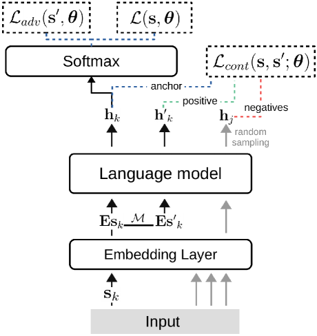
Figure 1: Basic architecture for our proposed approach. A batch $\mathbf{S}$ of sentences $\mathbf{s}_{k}$ are given as an input. After the embedding layer we compute the perturbed example in one of the randomly selected tokens from the mask $\mathcal{M}$. Both sentences are forwarded through the main model (in this case, language model.) Right before softmax, we apply contrastive loss to the representations of the forwarded sentences (original one $\mathbf{h}$ and perturbed one $\mathbf{h^{\prime}}$), and randomly sampled negatives from other sentences in the batch. Finally, we compute the three loses in Eq. 7 accordingly.

As shown in Figure 1, the original sentences and their adversarial counterparts (i.e., sentences in which the embedding of a token has been perturbed) are forwarded through the encoder to obtain the representation $\mathbf{h}_{k}$ and $\mathbf{h}^{\prime}_{k}$ right before the softmax layer. These representations have enough information to predict the next word, and they should have the same outcome, since they only differ in a small variation of one token embedding (Hahn and Choi 2019). However, the adversarial perturbation will move the representation away from the one of original sentence, we need to force the proximity of the representation using contrastive learning.

Taking the representation of the original candidate $\mathbf{h}_{kj}$ as the anchor point and its adversarial perturbed example $\mathbf{h}^{\prime}_{kj}$ as the positive, we define the contrastive loss like Eq. 4:

$$\mathcal{L}_{cont}=\sum_{\mathbf{h_{kj}}\in\mathbf{H(S)}}\mathcal{L}_{kj},$$ (5)

where

$$\mathcal{L}_{kj}=-\log\frac{\exp(cosim(\mathbf{h_{kj}},\mathbf{h^{\prime}_{kj}})/\tau)}{\sum_{\mathbf{h}_{n}\in\mathbf{NB}}\exp(cosim(\mathbf{h_{kj}},\mathbf{h}_{n})/\tau)},$$ (6)

where $cosim(\cdot,\cdot)$ is the cosine similarity of the representations, $\mathbf{NB_{kj}}\equiv\mathbf{H(S)}-\{h_{kj}\}$ are the batches of the sentence representations without the anchor point token’s, and $n$ is the number of negatives randomly sampled from this batch $\mathbf{H(S)}$. By sampling negatives from $\mathbf{H(S)}-\{\mathbf{h_{kj}}\}$, we make sure that the anchor point is not selected as a negative sample during each computation.

Finally, the objective of the ATCL is then computed by

$$\mathcal{J}(\boldsymbol{\theta})_{ATCL}=\sum_{\mathbf{s},\mathbf{s^{\prime}}}\bigg{(}\mathcal{L}+\alpha\mathcal{L}_{adv}+\beta\mathcal{L}_{cont}\bigg{)},$$ (7)

which is basically the same as Eq. 3, except that the adversarial examples are generated differently and the loss term $\mathcal{L}_{cont}$ is given by Eq. 6, considering language issues as described above.

4 Related work

To the best of our knowledge, adversarial training with contrastive learning has not been successful for natural language in general (Jaiswal et al. 2021).

Simultaneous to the development of our work, (Chen et al. 2021) proposed using the benefits of contrastive loss for adversarial training. In their work, they showed a disentangled contrastive learning method without using negative samples, and the experiments were carried out only with the BERT architecture. The main difference with our approach is the application of the contrastive learning method: the adversarial perturbations come from backtranslation models instead of an FGM, and the role of the negatives samples is replaced by the joint optimization of two sub-tasks (feature alignment and feature uniformity). Moreover, as the authors mentioned, their approach has some limitations that it works only with their contrastive sub-tasks that needs to be further explored in future works. Although some idea of their work may be shared with our approach, the execution of the method is completely different. Furthermore, our method provides a more general strategy for contrastive learning in adversarial settings that can be applied to any network architectures, not only BERT related tasks.

For ATCL, the challenge lies in the way of computing $\mathcal{L}_{rep}(\mathbf{h},\mathbf{h^{\prime}})$ for contrastive learning. The closest approach to our implementation is by (Cheng et al. 2018), where they used a CNN model as a discriminator (Kim 2014) to compute the loss $\mathcal{L}_{rep}$. Another example is (Cheng, Jiang, and Macherey 2019), which uses doubly adversarial examples, that is, the restriction in the representations is made by simultaneously training the encoding and decoding of the adversarial example using pre-trained language models. In this case, the loss $\mathcal{L}_{rep}$ is divided into two terms, for the source and the target languages, respectively. One of the drawbacks of these approaches is the additional training of these models, and the fact that they have to be pre-trained by other neural network architecture apart from the original task network. Our method computes this loss without any external pre-trained architecture and take advantage of the benefits of contrastive loss in a rather naive way. Our results show that this approach is beneficial to training models for language tasks.

5 Experiment

We experimented the proposed idea for language modeling (LM) and neural machine translation (NMT) tasks. The experiments were conducted using at core the Transformer model (Vaswani et al. 2017). For both tasks we computed only one adversarial sentence $\mathbf{s^{\prime}}$ per sentence $\mathbf{s}$ in the corpus. With adversarial sentence we refer to a sentence in which one of the embedded tokens has been replaced with a perturbed one.

5.1 Language Model

Language models (LMs) based on neural networks capture the syntactic and semantic language regularities (Bengio, Ducharme, and Vincent 2003; Mikolov et al. 2010). Thus, LMs can predict the probability of tokens $x_{i}$ given the predecessor sequence $\{x_{j}\}_{1<j<i-1}$ as conditional probability $p(x_{i}|x_{1},...,x_{i-1})$, or can calculate the likelihood of a given sentence. The likelihood which is a joint probability can be calculated with conditional probability as follows:

$$p(\mathbf{s}) = p(x_{1},x_{2},...,x_{T})$$ (8)

$$= p(x_{1})\prod_{i=2}^{T}p(x_{i}|x_{1},...,x_{i-1}).$$ (9)

We used the architecture of the Tensorized Transformer proposed by (Ma et al. 2019) which replaces the standard multi-head attention layers in the original Transformer with a Multi-linear attention. The Tensorized Transformer has significantly fewer parameters, in addition to achieving a better Perplexity (PPL) score than the original Transformer (Vaswani et al. 2017). We experimented in the Penn TreeBank (Mikolov et al. 2011) and WikiText-103 (Merity et al. 2016) datasets as summarized in Table 1.

	Train	Valid	Test
PTB	929k	73k	82k
Wiki-103	$\sim$103M	$\sim$218k	$\sim$246k

Table 1: Number of tokens for training/validation/test in the Penn TreeBank (PTB) and WikiText-103 (Wiki-103).

For both datastets, the hyperparameters $\epsilon$ (Eq. 1), $\alpha$, $\beta$ (Eq. 3) and the temperature coefficient $\tau$ (Eq. 6) were set to 0.03, 0.1, 0.1, and 0.07, respectively, and the batch size was 45.

Quantitative Results

For quantitative comparison, the perplexity scores of the LM task are presented in Table 2. To evaluate the effects of adversarial training and contrastive learning separately, on the Tensorized Transformer (TT) ‘Baseline TT’, we added adversarial training (‘+Adv. only’ which means $\beta=0$ in Eq. 7) and ATCL (‘+ATCL’). In general, ‘+ATCL’ improves the PPL scores significantly compare to the others. Note that ‘+Adv. only’ does not improve for Penn Tree Bank, though it does a little for Wikitext 103, which means that contrastive learning works effectively on the adversarial examples.

To check the effect of the number of negative samples in the contrastive loss (i.e., $n$ in Eq. 6.), we experimented with different amount of randomly sampled negatives from the batches. We can see that increasing the number is not always beneficial. For the WikiText-103 dataset, increasing the number of randomly sampled negatives gives a better PPL score. However, for a smaller dataset like PTB the adding more negatives harms the performance. We believe that the effect of the number of negative samples depends on the amount of unique tokens in the batch. PTB dataset has less number of unique tokes, which makes selecting “bad” negatives very plausible (tokens with no significant semantic impact).

Model and Training	Wikitext 103		Penn Tree Bank
	Validation	Test	Validation	Test
T with adaptive input*	19.80	20.50	59.10	57.00
T XL base*	23.10	24.00	56.72	54.52
T XL +TT *	23.61	25.70	57.90	55.40
Baseline TT	22.70	22.42	41.91	36.13
Baseline +Adv. only	21.75	21.67	42.68	36.46
Baseline +ATCL (n=5)	22.79	22.59	37.93	32.89
Baseline +ATCL (n=10)	21.75	21.67	35.29	29.08
Baseline +ATCL (n=20)	20.73	20.61	42.52	36.85

Table 2: Perplexity (PPL) of language model for the validation and test datasets. T stands for Transformer (Vaswani et al. 2017) and TT for Tensorized Transformer (Ma et al. 2019). We experimented based on our implementation, comparing them with other results using Transformer architectures given by (Ma et al. 2019) (*). We experimented our adversarial setting with (+ATCL) and without contrastive loss (+Adv. only), and in parenthesis we report the amount of negatives randomly sampled from the batch.

Word Representation

One of the advantages of contrastive learning is that it brings closer similar samples in the representation space, while pushing them further apart from different ones. We study this effect qualitatively in the text corpus.

After training, we computed the closest neighbors (by Euclidean distance) to the anchor words. In Table 3 we show the neighbors for three tokens after training the baseline, training only using FGM (i.e., ‘+Adv. only’), and with our proposed idea (‘+ATCL’). Surprisingly, we can observe that contrastive loss helps generate more semantic representation in the word-level. For example, for a word with negative connotations such as ‘hate’, its neighbors are negative words after contrastive learning. In contrast, the baseline model and training with only adversarial loss show a mix of synonyms and antonyms as neighbors of the anchor word. This suggests that the contrastive loss has the effect of rearranging the representation space with semantic information. By contrastive loss, words with similar embeddings are forced to be mapped to the same outcome, and at the same time, different representations are forced to be apart. This result in a semantic clustering that helps with the word-level semantics.

Word	Baseline	+Adv. only	+ATCL
friend	‘brother’, ‘daughter’, ‘understanding’, ‘director’	‘cousin’, ‘colleague’, ‘knowledge’, ‘mentor’	‘cousin’, ‘fellow’, ‘partner’, ‘colleague’
hate	‘admit’, ‘prejudice’, ‘troubled’, ‘regret’	‘loving’, ‘hurt’, ‘embrace’, ‘committing’	‘dirty’, ‘poison’, ‘regret’, ‘shame’
like	‘under’, ‘so’, ‘offering’, ‘@.@’	‘under’, ‘inspired’, ‘less’, ‘led’	‘before’, ‘just’, ‘alongside’, ‘despite’

Table 3: Four closest neighbors of some words in the vocabulary of the WikiText-103 dataset after training with the baseline (refer to Table 2), with only the adversarial loss, and with our proposed training loss (Eq. 6). In bold, we marked the words with different connotation from the anchor word. We observe that the contrastive loss promotes some qualitative improvement in the word-level representation.

Robustness Against Attacks

We also conducted a qualitative study of targeted adversarial attacks. Given a sentence from the test set, we perturbed the embedding of a target word following the method described in Section 2.1. This word is around the end of the sentence and they should be meaningful (we used the mask criteria $\mathcal{M}$ explained before.) The set of the perturbed sentences was forwarded through the baseline model and our proposed model, and the models complete the sentence after the perturbed word with the predicted probability for the next words.

Some generated results are presented in Table 4, where in most cases, our proposed approach yields better predictions than the baseline model. For example, the first result shows that our model generates nicely “a starring support role”, while the baseline generates “a starring joint television”, which is broken due to the targeted attack. The average perplexities of the generated sentences from the baseline and from our ‘+ATCL’, are 10.12 and 8.77, respectively. Thus, after applying the perturbations, the generated sentences from the ATCL have produced a lower loss in the trained model than the ones generated from the baseline. Note that even though we trained our model to be resistant of perturbations in sentence-level, the results show that it is also robust against targeted perturbation in the word-level.

Baseline	He had a guest @-@ starring role on the television series The Bill in 2000 . This was followed by a starring join television.
+ATCL	He had a guest @-@ starring role on the television series The Bill in 2000 . This was followed by a starring support role.
Baseline	The massive North Korean attack had made deep penetrations everywhere in the division sector except in the north in the zone of city.
+ATCL	The massive North Korean attack had made deep penetrations everywhere in the division sector except in the north in the zone of town.
Baseline	Hall was involved for one month during preproduction; his ideas for lighting the film began with his first reading of the script, and further passes allowed him to refine his approach before other sunk.
+ATCL	Hall was involved for one month during preproduction; his ideas for lighting the film began with his first reading of the script, and further passes allowed him to refine his approach before other shot.
Baseline	However , they are rarely considered for a modern design , the principles behind them having been superseded by other methodologies which are more accurate design that $<$unk$>$.
+ATCL	However , they are rarely considered for a modern design , the principles behind them having been superseded by other methodologies which are more accurate patent of elements.

Table 4: Examples of next word prediction after adversarially perturbing the embedding of a token in a sequence. In bold, we marked the words that were perturbed by following the Eq. 1, and in italic, the predicted tokens by the differently trained models (baseline and ours.) Our approach completes sentences which make more sense given the context than the baseline.

5.2 Neural Machine Translation

Neural machine translation (NMT) consists of processing tokens in a certain source language and predicting the corresponding sequence of tokens in a target language based on encoder and decoder with end-to-end training (Sutskever, Vinyals, and Le 2014; Bahdanau, Cho, and Bengio 2015). That is, given a sequence $\mathbf{s^{src}}=\{x_{1},x_{2},...,x_{D}\}$, it is mapped to a target sequence $\mathbf{s^{trg}}=\{y_{1},y_{2},...,y_{M}\}$. In general, the objective of NMT is to maximize the conditional probability as follows

$$p(\mathbf{s^{trg}}|\mathbf{s^{src}})=\prod^{M}_{m=1}p(y_{m}|y_{<m},\mathbf{s^{src}};\boldsymbol{\theta}),$$ (10)

where the parameter $\boldsymbol{\theta}$ is updated to maximize the conditional probability.

We experimented with the IWSLT’17 datasets for English-German (En-De) and English-French (En-Fr) pairs. Both datasets are segmented using the Byte-Pair Encoding (BPE) method (Sennrich, Haddow, and Birch 2015). Since we only choose one token to adversarially perturb per sentence, we only considered as adversarial candidates complete word tokens (i.e., not subwords) using the mask $\mathcal{M}$. The details of each language pair dataset are shown in Table 5.

	Train	Valid	Test	Vocab	BPE tok
En-De	$\sim$160k	$\sim$7k	$\sim$6k	10k (s)	36.63%
En-Fr	$\sim$200k	$\sim$7k	$\sim$6k	28k (ns)	24.34%

Table 5: Details of amount of parallel corpus sentences for En-De and En-Fr training, validation, and test sets. We also show the vocabulary length (and in parenthesis if it is shared or not shared) and the percentage of subwords in the vocabulary.

For the NMT experiments we used the same configurations of (Vaswani et al. 2017) except for the number of layers in the encoder and decoder. Since there was no significant difference in performance, for these datasets we used 3 layers instead of 6.

Results

The experiments for the NMT task were carried out in a similar modality as the LM task. We show the result of different configurations for each of the language pairs in Table 6. Again, we tried with different number of negatives. We can see that ATCL increases the BLEU score compared to the baseline, though the improvement is not as significant as in LM. There is some cases like ‘Fr-En’, training with only the adversarial loss gives a slightly better performance than ATCL.

Model name	En-De	De-En	En-Fr	Fr-En
Baseline (Transformer S)	24.61	30.34	35.23	34.51
Baseline +Adv	25.04	30.36	35.02	35.97
Baseline +ATCL	24.63	31.34	36.40	35.35
	25.26	30.36	35.60	35.48
	24.74	30.13	35.38	35.46

Table 6: BLEU test scores for the IWSLT dataset (we used IWSLT15’ as testing datasets.). ‘Baseline + ATCL’ has 3 results with 5, 10 and 20 negative samples as in LM.

As shown in Table 6, the advantages of using the contrastive loss for NMT task are less visible. We speculate that the main reason of this lack of improvement is the use of BPE. Our approach relies heavily on embedding similarity, i.e. we perform the experiments under the assumption that similarity (closeness) in the word representation space involves semantic similarity. In this case, the training is harmed by this assumption. The representation of subwords due to BPE in the embedding space is less straightforward to understand than in the LM task. Even though we masked the input sentences so that we could only choose complete words, when sampling the negatives from the batch we do not rely on this mask. Thus, contrastive loss might be partly based on some meaningless subwords for negative samples which can diminish the advantage of contrastive learning for semantic representation.

We also show some qualitative results in Table 7. Given the source (src) and target (trg) sentences, we show some translations for the En-De language pairs using the baseline (Baseline) and our model (ATCL). The latter shows some semantic improvement in the quality of the translations.

Example from De-En
src (De)	Und ich dachte mir : “wow , das muss unbedingt in die filmkunst einbezogen werden.”
trg (En)	And I thought , “wow , this is something that needs to be embraced into the cinematic art.”
Baseline	And I thought to myself , “wow , this may have been reluctant to the movie.”
Adv.	And I thought , “wow , this has to be very much involved in filmmaking.”
ATCL	and i thought , “wow , this is something that needs to be involved in film art.”
Example from Fr-En
src (Fr)	Voici Toxoplasma gondii, ou Toxo pour les amis, parce qu’une créature terrifiante à toujours droit à un
	joli surnom.
trg (En)	This is Toxoplasma gondii, or Toxo, for short, because the terrifying creature always deserves a cute
	nickname.
Baseline	This is Toxo, or Toxo from friends, because a terrifying creature to a Beautiful nickname.
Adv.	This is Toxo, or Toxo from friends, because a terrifying creature is always right for a beautiful nickname.
ATCL	This is Toxo, or Toxo from friends, because a terrifying creature is always right for a beautiful nickname.

Table 7: Examples of De-En and Fr-En translations after perturbing the embedding of some tokens (in bold) in the source (src). We show the translations of the target sentence (trg), the baseline model (Baseline), the model trained with only adversarial perturbations (Adv.), and our approach (ATCL). These examples show that our model seems to capture better the underlying semantic meaning of the source sentence than the baseline. However, there are some cases in which the results are similar between Adv. and ATCL, also reflected in the BLEU scores results of Table 6.

6 Conclusion and Future Work

In this work we proposed a simple idea for combining the advantages of the contrastive learning to adversarial training in language tasks. Our approach was applied to language modeling and neural machine translation tasks with promising results. We show some benefits of forcing the proximity of the representations of the original tokens and their adversarial ones via contrastive learning. We believe this to be a simple approach to train NLP models adversarially without the use of a pre-trained models or any limit on the model architecture.

This implementation can be improved further in some ways. First, random sampling from a batch may not be the optimal strategy for obtaining negatives. Even though we show that for the LM task training with these negatives gives a lower PPL score, we believe that further improvements can be achieved with negatives carefully crafted according to semantics. Another question is if contrastive learning can be applied to representation spaces in which the “similarity” concept is not easy to interpret, like in language settings, where cosine similarity may be too simple. Future works should include a thorough study on better similarity measures.

Despite these limitations, we believe this to be a first approach to introduce the benefits of contrastive learning into adversarial training for language tasks without the use of external pre-trained models.

References

- Alzantot et al. (2018) Alzantot, M.; Sharma, Y.; Elgohary, A.; Ho, B.-J.; Srivastava, M.; and Chang, K.-W. 2018. Generating natural language adversarial examples. arXiv preprint arXiv:1804.07998.
- Bahdanau, Cho, and Bengio (2015) Bahdanau, D.; Cho, K.; and Bengio, Y. 2015. Neural Machine Translation by Jointly Learning to Align and Translate. In iclr.
- Bengio, Ducharme, and Vincent (2003) Bengio, Y.; Ducharme, R.; and Vincent, P. 2003. A Neural Probabilistic Language Model. The Journal of Machine Learning Research, 3: 1137–1155.
- Chen et al. (2020) Chen, T.; Kornblith, S.; Norouzi, M.; and Hinton, G. 2020. A simple framework for contrastive learning of visual representations. In International conference on machine learning, 1597–1607. PMLR.
- Chen et al. (2021) Chen, X.; Xie, X.; Bi, Z.; Ye, H.; Deng, S.; Zhang, N.; and Chen, H. 2021. Disentangled Contrastive Learning for Learning Robust Textual Representations. arXiv preprint arXiv:2104.04907.
- Cheng, Jiang, and Macherey (2019) Cheng, Y.; Jiang, L.; and Macherey, W. 2019. Robust neural machine translation with doubly adversarial inputs. arXiv preprint arXiv:1906.02443.
- Cheng et al. (2018) Cheng, Y.; Tu, Z.; Meng, F.; Zhai, J.; and Liu, Y. 2018. Towards robust neural machine translation. arXiv preprint arXiv:1805.06130.
- Chopra, Hadsell, and LeCun (2005) Chopra, S.; Hadsell, R.; and LeCun, Y. 2005. Learning a similarity metric discriminatively, with application to face verification. In 2005 IEEE Computer Society Conference on Computer Vision and Pattern Recognition (CVPR’05), volume 1, 539–546. IEEE.
- Dong et al. (2018) Dong, Y.; Liao, F.; Pang, T.; Su, H.; Zhu, J.; Hu, X.; and Li, J. 2018. Boosting adversarial attacks with momentum. In Proceedings of the IEEE conference on computer vision and pattern recognition, 9185–9193.
- Duan et al. (2019) Duan, X.; Yu, H.; Yin, M.; Zhang, M.; Luo, W.; and Zhang, Y. 2019. Contrastive attention mechanism for abstractive sentence summarization. arXiv preprint arXiv:1910.13114.
- Ebrahimi, Lowd, and Dou (2018) Ebrahimi, J.; Lowd, D.; and Dou, D. 2018. On adversarial examples for character-level neural machine translation. arXiv preprint arXiv:1806.09030.
- Garg and Ramakrishnan (2020) Garg, S.; and Ramakrishnan, G. 2020. Bae: Bert-based adversarial examples for text classification. arXiv preprint arXiv:2004.01970.
- Giorgi et al. (2020) Giorgi, J. M.; Nitski, O.; Bader, G. D.; and Wang, B. 2020. Declutr: Deep contrastive learning for unsupervised textual representations. arXiv preprint arXiv:2006.03659.
- Goodfellow, Shlens, and Szegedy (2014) Goodfellow, I. J.; Shlens, J.; and Szegedy, C. 2014. Explaining and harnessing adversarial examples. arXiv preprint arXiv:1412.6572.
- Hahn and Choi (2019) Hahn, S.; and Choi, H. 2019. Self-Knowledge Distillation in Natural Language Processing. In Proceedings of the International Conference on Recent Advances in Natural Language Processing (RANLP 2019), 423–430. Varna, Bulgaria: INCOMA Ltd.
- He et al. (2020) He, K.; Fan, H.; Wu, Y.; Xie, S.; and Girshick, R. 2020. Momentum contrast for unsupervised visual representation learning. In Proceedings of the IEEE/CVF Conference on Computer Vision and Pattern Recognition, 9729–9738.
- Henaff (2020) Henaff, O. 2020. Data-efficient image recognition with contrastive predictive coding. In International Conference on Machine Learning, 4182–4192. PMLR.
- Hjelm et al. (2018) Hjelm, R. D.; Fedorov, A.; Lavoie-Marchildon, S.; Grewal, K.; Bachman, P.; Trischler, A.; and Bengio, Y. 2018. Learning deep representations by mutual information estimation and maximization. arXiv preprint arXiv:1808.06670.
- Jaiswal et al. (2021) Jaiswal, A.; Babu, A. R.; Zadeh, M. Z.; Banerjee, D.; and Makedon, F. 2021. A survey on contrastive self-supervised learning. Technologies, 9(1): 2.
- Jin et al. (2020) Jin, D.; Jin, Z.; Zhou, J. T.; and Szolovits, P. 2020. Is bert really robust? a strong baseline for natural language attack on text classification and entailment. In Proceedings of the AAAI conference on artificial intelligence, volume 34, 8018–8025.
- Khosla et al. (2020) Khosla, P.; Teterwak, P.; Wang, C.; Sarna, A.; Tian, Y.; Isola, P.; Maschinot, A.; Liu, C.; and Krishnan, D. 2020. Supervised contrastive learning. arXiv preprint arXiv:2004.11362.
- Kim (2014) Kim, Y. 2014. Convolutional neural networks for sentence classification. EMNLP.
- Kurakin et al. (2016) Kurakin, A.; Goodfellow, I.; Bengio, S.; et al. 2016. Adversarial examples in the physical world.
- Logeswaran and Lee (2018) Logeswaran, L.; and Lee, H. 2018. An efficient framework for learning sentence representations. arXiv preprint arXiv:1803.02893.
- Ma et al. (2019) Ma, X.; Zhang, P.; Zhang, S.; Duan, N.; Hou, Y.; Zhou, M.; and Song, D. 2019. A tensorized transformer for language modeling. Advances in Neural Information Processing Systems, 32: 2232–2242.
- Merity et al. (2016) Merity, S.; Xiong, C.; Bradbury, J.; and Socher, R. 2016. Pointer sentinel mixture models. arXiv preprint arXiv:1609.07843.
- Mikolov et al. (2011) Mikolov, T.; Deoras, A.; Kombrink, S.; Burget, L.; and Černockỳ, J. 2011. Empirical evaluation and combination of advanced language modeling techniques. In Twelfth annual conference of the international speech communication association.
- Mikolov et al. (2010) Mikolov, T.; Karafiat, M.; Burget, L.; Cernocky, J.; and Khudanpur, S. 2010. Recurrent neural network based language model. In INTERSPEECH 2010, 11th Annual Conference of the International Speech Communication Association, 1045–1048.
- Miyato, Dai, and Goodfellow (2016) Miyato, T.; Dai, A. M.; and Goodfellow, I. 2016. Adversarial training methods for semi-supervised text classification. arXiv preprint arXiv:1605.07725.
- Moosavi-Dezfooli, Fawzi, and Frossard (2016) Moosavi-Dezfooli, S.-M.; Fawzi, A.; and Frossard, P. 2016. Deepfool: a simple and accurate method to fool deep neural networks. In Proceedings of the IEEE conference on computer vision and pattern recognition, 2574–2582.
- Morris (2020) Morris, J. X. 2020. Second-Order NLP Adversarial Examples. arXiv preprint arXiv:2010.01770.
- Papernot et al. (2016) Papernot, N.; McDaniel, P.; Jha, S.; Fredrikson, M.; Celik, Z. B.; and Swami, A. 2016. The limitations of deep learning in adversarial settings. In 2016 IEEE European symposium on security and privacy (EuroS&P), 372–387. IEEE.
- Pappas and Henderson (2019) Pappas, N.; and Henderson, J. 2019. Gile: A generalized input-label embedding for text classification. Transactions of the Association for Computational Linguistics, 7: 139–155.
- Ren et al. (2019) Ren, S.; Deng, Y.; He, K.; and Che, W. 2019. Generating natural language adversarial examples through probability weighted word saliency. In Proceedings of the 57th annual meeting of the association for computational linguistics, 1085–1097.
- Rethmeier and Augenstein (2020) Rethmeier, N.; and Augenstein, I. 2020. Long-tail zero and few-shot learning via contrastive pretraining on and for small data. arXiv e-prints, arXiv–2010.
- Rethmeier and Augenstein (2021) Rethmeier, N.; and Augenstein, I. 2021. A Primer on Contrastive Pretraining in Language Processing: Methods, Lessons Learned and Perspectives. arXiv preprint arXiv:2102.12982.
- Sennrich, Haddow, and Birch (2015) Sennrich, R.; Haddow, B.; and Birch, A. 2015. Neural machine translation of rare words with subword units. arXiv preprint arXiv:1508.07909.
- Sutskever, Vinyals, and Le (2014) Sutskever, I.; Vinyals, O.; and Le, Q. V. 2014. Sequence to Sequence Learning with Neural Networks. In nips.
- Szegedy et al. (2013) Szegedy, C.; Zaremba, W.; Sutskever, I.; Bruna, J.; Erhan, D.; Goodfellow, I.; and Fergus, R. 2013. Intriguing properties of neural networks. arXiv preprint arXiv:1312.6199.
- Tian, Krishnan, and Isola (2020) Tian, Y.; Krishnan, D.; and Isola, P. 2020. Contrastive multiview coding. In Computer Vision–ECCV 2020: 16th European Conference, Glasgow, UK, August 23–28, 2020, Proceedings, Part XI 16, 776–794. Springer.
- Vaswani et al. (2017) Vaswani, A.; Shazeer, N.; Parmar, N.; Uszkoreit, J.; Jones, L.; Gomez, A. N.; Kaiser, Ł.; and Polosukhin, I. 2017. Attention is all you need. In Advances in neural information processing systems, 5998–6008.
- Wu et al. (2018) Wu, Z.; Xiong, Y.; Yu, S. X.; and Lin, D. 2018. Unsupervised feature learning via non-parametric instance discrimination. In Proceedings of the IEEE conference on computer vision and pattern recognition, 3733–3742.
- Zhang et al. (2020) Zhang, W. E.; Sheng, Q. Z.; Alhazmi, A.; and Li, C. 2020. Adversarial attacks on deep-learning models in natural language processing: A survey. ACM Transactions on Intelligent Systems and Technology (TIST), 11(3): 1–41.