Abstract

High energy photons from astrophysical sources are unique probes for some predictions of candidate theories of Quantum Gravity (QG). In particular, imaging atmospheric Cherenkov telescopes are instruments optimised for astronomical observations in the energy range spanning from a few tens of GeV to $\sim$100 TeV, which makes them excellent instruments to search for effects of QG. In this article, we will review QG effects which can be tested with IACT, most notably the Lorentz invariance violation (LIV) and its consequences. It is often represented and modelled with photon dispersion relation modified by introducing energy-dependent terms. We will describe the analysis methods employed in the different studies, allowing for careful discussion and comparison of the results obtained with IACT for more than two decades. Loosely following historical development of the field, we will observe how the analysis methods were refined and improved over time, and analyse why some studies were more sensitive than others. Finally, we will discuss the future of the field, presenting ideas for improving the analysis sensitivity and directions in which the research could develop.

Content

section.1subsection.1.1subsection.1.2section.2subsection.2.1subsection.2.2subsection.2.3subsection.2.4subsection.2.5subsection.2.6subsection.2.7subsection.2.8subsection.2.9subsection.2.10subsection.2.11subsection.2.12subsection.2.13section.3subsection.3.1subsubsection.3.1.1subsubsection.3.1.2subsubsection.3.1.3subsubsection.3.1.4subsection.3.2subsection.3.3section.4section.5subsection.5.1subsection.5.2subsection.5.3section.6

1 Introduction and Motivation

The general theory of relativity is a beautiful and elegant theory, which connects the local matter and energy content to the curvature of spacetime, thus giving a classical description of gravity. It has been heavily tested and scrutinised ever since Albert Einstein proposed it in 1915 Einstein (1916). Nevertheless, it breaks down in extreme circumstances such as singularities within black holes, or the early universe. Therefore, it is expected that there exists a more fundamental quantum theory of gravity, which can handle these extreme situations. Furthermore, a quantum theory of gravity would be a giant leap towards unification of all fundamental forces.

Theoretical endeavours in formulating the theory of QG have explored different avenues (see, e.g., Rovelli and Smolin (1990); Rovelli (2007); Oriti (2001); Niedermaier and Reuter (2006); Ambjorn et al. (2012); Horowitz (2005)). However, despite significant efforts, a complete and consistent description of gravity on a quantum level remains unknown. In addition, many of the QG models include departures form the Lorentz symmetry (see, e.g., Kostelecky and Samuel (1989); Gambini and Pullin (1999); Carroll et al. (2001); Douglas and Nekrasov (2001)). Performing measurements in the expected realm of QG would strongly hint in which direction theoretical research should proceed. Unfortunately, the expected domain of QG is the Planck scale . Even if QG emerges at energies several orders of magnitude below $E_{\mathrm{Pl}}$, it is still vastly above the highest energies accessible in contemporary human-built accelerators. When technology falls short, we turn to nature’s own accelerators: active galactic nuclei, gamma-ray bursts, supernova remnants, pulsars, etc. The most energetic particles detected up to date, a cosmic ray at $\sim$$3.2\times 10^{11}$ GeV Bird et al. (1995); Halzen et al. (1995), a neutrino at $\sim$$6.3\times 10^{6}$ GeV Aartsen et al. (2021), and a gamma ray at $\sim$$1.4\times 10^{6}$ GeV Cao et al. (2021), while reaching energies higher than those achievable in Earth-based accelerators, are still more than a little shy of $E_{\mathrm{Pl}}$. So what allows us to hope that we will measure an effect of QG?

1.1 A Proposal to Probe Quantum Gravity

In 1997, the distance of a gamma-ray burst (GRB) was measured for the first time. Indeed, following the detection of GRB 970508 Costa et al. (1997), an optical counterpart was observed Djorgovski et al. (1997), which allowed estimating of its redshift to $0.835\leq z\lesssim 2.3$ Metzger et al. (1997). A strong flux of gamma rays from a quickly varying source detected at a cosmological distance incited Amelino-Camelia et al. Amelino-Camelia et al. (1998) to suggest that the signal from GRBs could be used to probe the structure of spacetime. The proposal was based on the idea of spacetime as a dynamical medium, which experiences quantum fluctuations due to QG effects. While the scale of fluctuations was expected to be comparable to the Planck units, propagation of photons of substantially smaller energies could still be affected by it. Probing the fluctuations would result in an energy-dependent propagation speed, similar to what visible light experiences when propagating through a medium such as water or air.

1.2 Modified Photon Dispersion Relation

This behaviour can be modelled by modifying the standard photon dispersion relation in the following way:

$$E^{2}=p^{2}c^{2}\times\left[1+\sum_{n=1}^{\infty}S_{n}\left(\frac{E}{E_{\mathrm{QG,}n}}\right)^{n}\right],$$ (1)

where $E$ and $p$ are respectively the energy and momentum of a photon, $c$ is the Lorentz invariant speed of light, and the $E_{\mathrm{QG,}n}$ are the energy scales at which effects of QG become significant. We will start discussing the values of $E_{\mathrm{QG,}n}$ in a short while, for now let us just acknowledge that $E/E_{\mathrm{QG,}n}\ll 1$ even for the most energetic gamma rays. Different modifying terms in the dispersion relation contribute less and less with increasing $n$. Therefore, usually, only the first two leading terms ($n=1$ or $n=2$) of the series are considered and independently tested for. They are often referred to as linear and quadratic energy-dependent contributions, respectively. Letting $E_{\mathrm{QG,}n}\rightarrow\infty$ for all $n$ leads to the well-known Lorentz invariant photon dispersion relation. Parameters $S_{n}$ can take values $\pm 1$, and their role will become apparent immediately. From Equation (1) the energy-dependent photon group velocity can be easily derived as:

$$v_{\gamma}=\frac{\partial E}{\partial p}\simeq c\left[1+\sum_{n=1}^{\infty}S_{n}\frac{n+1}{2}\left(\frac{E}{E_{\mathrm{QG,}n}}\right)^{n}\right].$$ (2)

Considering each modifying term independently, one can see that for $S_{n}=+1$, the velocity becomes greater than $c$, while for $S_{n}=-1$ it becomes smaller than $c$. These two behaviours are known as superluminal and subluminal, respectively.

Once a modification is introduced in the dispersion relation, various effects (other than changes in the photon speed) are conceivable, such as the modification of the electromagnetic interaction. But whatever the effects of modifying the dispersion relation may be, they are minuscule because of the ratio $E/E_{\mathrm{QG,}n}$. The good news, however, is that the effects are cumulative. This is extremely important because gamma rays from some astrophysical sources take billions of years to reach Earth, allowing for these potential effects to accumulate, thus giving hope that we might be able to measure their consequences from Earth.

Additionally, the effects of modifying the dispersion relation are more pronounced for higher energy photons. Thus, searching for them with IACT, which are instruments optimised for astronomical observations in the very high energy (VHE) gamma-ray band (100 GeV $<E<$ 100 TeV), is a sensible thing to do. Given their large collection area and good sensitivity, IACT are excellent instruments for testing effects of QG on gamma rays, and will be the main focus of this review. At lower energies, satellite-born detectors such as the Fermi- Large Area Telescope (LAT) benefit from more distant observations, but suffer from their lower effective area (see Sections 2.13 and 4 for a brief comparison with the IACT results). On the other hand, at higher energies water Cherenkov detectors such as High Altitude Water Cherenkov (HAWC) or Large High Altitude Air Shower Observatory (LHAASO) have an advantage of observing in a higher energy range than IACT. However, due to the rapid decrease of the flux of gamma rays at these energies they are handicapped by smaller statistics, which makes them less sensitive to fast flux variations (see Sections 3.3 and 4 for a brief comparison with the IACT results).

Before taking a dive into the methods and results of probing QG with IACT, let us acknowledge that the modified photon dispersion relation is the usual starting point of experimental tests of QG on gamma rays. While some QG models indeed do not preserve Lorentz symmetry, it is important to note that Equation (1) is not a direct consequence of any particular QG model. Given that there is no fully formulated theory of QG, it would be overambitious to expect exact predictions. Rather, the modified dispersion relation can be regarded as a simple way of parameterizing and modelling phenomena not predicted by the current physical theories and laws. It, therefore, enables us to experimentally search for effects of those phenomena.

That being said, there are two main ways of modifying the dispersion relation that are usually considered. LIV, the main focus of this review, implies the existence of a preferred inertial frame of reference, which breaks the Lorentz symmetry Colladay and Kostelecky (1998). However, there are also ways of modifying the photon dispersion relation, while at the same time preserving the Lorentz symmetry. One example is the so-called Doubly Special Relativity (DSR) Amelino-Camelia (2002, 2010). In this model, the symmetry is deformed, rather than broken, and there is no preferred inertial frame of reference. Moreover, in order to keep the conservation laws covariant with respect to deformed symmetries of DSR, the conservation laws themselves need to be modified. This fundamental difference between LIV and DSR becomes important when different possible effects of QG are discussed. In particular, the kinematics, and possibly the dynamics, of electromagnetic interactions in the LIV framework will differ from the Lorentz invariant ones. In the DSR framework, on the other hand, the descriptions of interactions will be the same as (or only slightly different from) the Lorentz invariant descriptions. DSR is a recently discussed promising avenue of research gaining attention and traction. However, there has been no published results from IACT mentioning explicitly DSR effects thus far. Therefore, in the rest of the text, we will, refer to all effects as LIV, regardless of their true origin. We will, however, keep using $E_{\mathrm{QG,}n}$ to note the energy scales at which the effects become relevant. The details of either of these models, and their differences are out of the scope of this work. An interested reader is referred to a review paper by the COST Action 18108 (in preparation) and references therein.

In this paper, we will focus on searches for signatures of LIV in measurements with IACT. We will discuss various effects of modifying the photon dispersion relation and their respective probes, adopting a chronological course. However, it is our intention (instead of simply recalling the most important studies performed) to analyse the evolution of the field, with a particular focus on the development of the analysis methods. Hopefully, this approach will inspire the authors and the readers alike to formulate new ideas on how to search for the effects of QG, and pave the path for future research. Historically, the first effect to be tested was the energy dependence of the photon group velocity, so results of different measurements of the photon time of flight will be covered first, in Section 2. As stated above, LIV can affect the kinematics and dynamics of electromagnetic interactions. This other important class of effects will be discussed in Section 3. We might as well break the suspense and state right away that no effects of QG have been detected so far. Nevertheless, strong constraints have been set on the minimum value of the LIV energy scale. These are usually expressed as lower limits at the 95% confidence level. The results of different effects, obtained from various experiments and analysis methods will be mutually compared and their differences discussed in Section 4. Finally, we turn towards the future in Section 5, to discuss opportunities for development and progress of this field of research.

2 Testing Energy-Dependent Photon Group Velocity

Assuming energy-dependent propagation speeds, two photons of energies $E_{\mathrm{2}}>E_{\mathrm{1}}$ emitted from a source at the same time will have different, energy-dependent, times of flight $t^{\prime}_{2}$ and $t^{\prime}_{1}$ respectively, finally reaching Earth with an energy-dependent time delay Jacob and Piran (2008):

$$\Delta t^{\prime}=t^{\prime}_{2}-t^{\prime}_{1}=t\frac{\Delta v_{\gamma}}{c}\simeq-S_{n}\frac{n+1}{2}\frac{E_{\mathrm{2}}^{n}-E_{\mathrm{1}}^{n}}{E_{\mathrm{QG,}n}^{n}}D_{n}(z_{\mathrm{s}}),$$ (3)

where $t$ is the time needed for a photon travelling with speed $c$ to reach the Earth. The time delay is proportional to a source distance parameter:

$$D_{n}(z_{\mathrm{s}})=\frac{1}{H_{0}}\bigintss_{0}^{z_{\mathrm{s}}}\frac{(1+z)^{n}}{\sqrt{\Omega_{\mathrm{m}}\left(1+z\right)^{3}+\Omega_{\Lambda}}}dz,$$ (4)

where $z_{\mathrm{s}}$ is the source redshift, and $H_{0}$, $\Omega_{\mathrm{m}}$, and $\Omega_{\Lambda}$ represent cosmological parameters, respectively: the Hubble constant, the matter density parameter, and the dark-energy density parameter. The time delay expression was derived from comoving trajectories of particles, starting from their modified dispersion relations. More general and alternative expressions can be obtained by modifying the general relativistic dispersion relation as was done in Pfeifer (2018), or by adopting that the spacetime translations are modified alongside with the modification of the dispersion relation Rosati et al. (2015).

2.1 The First Test with an Imaging Atmospheric Cherenkov Telescope

Soon after it was proposed that GRBs could be used to search for effects of LIV, the first test using data from IACT was performed. In fact, researchers observing with the Whipple telescope already had a suitable data set available. Albeit, the source was not a GRB, but the very first active galactic nucleus (AGN) ever detected in the VHE gamma-ray band, Markarian 421 (Mrk 421, redshift $z=0.031$) Punch et al. (1992). On 15 May 1996, Whipple observed the most rapid flare from Mrk 421 up to that time, with the flux doubling time of less than 15 minutes and including photons of energies up to several TeV Gaidos et al. (1996). This groundbreaking study used a rather rudimentary analysis: the data set was split in two energy bands ($E<1$ TeV and $E>2$ TeV) Biller et al. (1999). In each energy band, the events were further subdivided in time bins of 280 s. The distribution of arrival times of photons with energies $E>2$ TeV was compared to the distribution of arrival times of events below 1 TeV. The authors used the likelihood-ratio test to compare the contents of time bins in the two energy ranges. In this study, no distinction was made between the subluminal and the superluminal behaviour. No delay in either direction was detected at the 95% confidence level. Combined with the distance to Mrk 421, this result was translated into a lower limit on the LIV energy scale $E_{\mathrm{QG,1}}>4\times 10^{16}$ GeV. Only the linear contribution was considered in this first study.

2.2 Fastest Variability in Blazars

The observation of Mrk 421 with the Whipple telescope drew attention to flaring blazars as possible probes of LIV. In the summer of 2005, the Major Atmospheric Gamma Imaging Cherenkov (MAGIC) telescopes observed two flares from the AGN Markarian 501 (Mrk 501, redshift $z=0.034$) Albert et al. (2007). The data analysis revealed that the flux doubled in only 2 minutes, which remains until today the fastest flux variability ever observed from a blazar in the VHE gamma-ray band. With the highest energies reaching $\sim$$10$ TeV, the flux varying by an order of magnitude, it was a chance not to be missed. Moreover, there was an indication of a $4\pm 1$ min delay between the peaks in the light curves in the lowest (0.15–0.25 TeV) and the highest (1.2–10 TeV) energy bins on the 9th of July. A search for an energy-dependent photon time of flight in the Mrk 501 flare of this night was performed employing two distinct statistical analysis methods which we will now describe.

ECF method utilises the fact that a signal pulse propagating through a dispersive medium will be diluted, and its power (total energy per unit time), consequently, decreased (see, e.g., Section 7.9 in Jackson (1999)). In the case of the Mrk 501 flare MAGIC Collaboration et al. (2008), the data sample was chosen by selecting the most active part of the flare, i.e., the time interval in which the temporal distribution of events differs the most from a uniform distribution. We will mark the beginning and the end of this time interval as $t_{1}$ and $t_{2}$, respectively. The power of the signal was calculated as the sum of the energies of all the photons within the interval divided by the duration of the interval. Had the photons experienced any energy-dependent time delay, the power would have been smaller than without dispersion. One can then search for the maximal possible power by applying dispersion in the opposite direction, assuming different values of the LIV energy scale. Specifically, in order to compute a new signal power, a new arrival time $t^{\prime}_{\mathrm{i}}$ was calculated for each photon in the sample for a particular value of $E_{\mathrm{QG,}n}$:

$$t^{\prime}_{\mathrm{i}}=t_{\mathrm{i}}+\eta_{n}E_{\mathrm{i}}^{{n}},$$ (5)

where $t_{\mathrm{i}}$ and $E_{\mathrm{i}}$ are, respectively, the measured arrival time and the measured energy of the $i$-th photon. Given the large values of $E_{\mathrm{QG,}n}$, various parameters are often introduced to facilitate numerical computations. Here the parameters $\eta_{{n}}$ is defined from Equation (3) as:

$$\eta_{n}=-S_{n}\frac{n+1}{2}\frac{1}{E_{\mathrm{QG,}n}^{n}}D_{n}(z_{\mathrm{s}}).$$ (6)

This parameter is introduced for computational reasons because $\eta_{n}$ is $\mathcal{O}(1)$. Usually expressed in units of [s/GeV] (for $n=1$) or [s/GeV²] (for $n=2$), $\eta_{{n}}$ indicates how much a photon will be delayed in arrival compared to a photon propagating at $c$ per every GeV of its energy. Limits on $E_{\mathrm{QG,}n}$ are then derived by inverting Equation (6).

The arrival time recalculation as described in Equation (5) was performed for each individual gamma ray, and only photons whose recalculated arrival times fell in the $[t_{1},t_{2}]$ time interval were retained. In this way, an alternative sample of photons was constituted, and its total energy calculated. The procedure was repeated for different values of $\eta_{n}$ (i.e., different values of $E_{\mathrm{QG,}n}$). The energy cost function (ECF) was defined as the total energy as a function of $\eta_{n}$. The value of $\eta_{n}$ which maximises the ECF, would recover the maximal signal power. In other words, it would correspond to the measurement of the dispersion which the gamma rays experienced because of the LIV effects, assuming no other effects play a significant role. The sensitivity of the method and the confidence interval for parameters $\eta_{n}$ were estimated using Monte Carlo simulations of the observed signal. Next, 1000 of simulated data sets were generated, and the ECF method was applied to each of them. The most probable value of $\eta_{n}$ and its confidence interval were estimated from the distribution of $\eta_{n}$, which were then translated into lower limit on the LIV energy scale at the 95% confidence level. This particular analysis yielded $E_{\mathrm{QG,1}}>2.1\times 10^{17}$ GeV, which was more constraining than the Whipple result on Mrk 421 flare from 1996 Biller et al. (1999) by an order of magnitude. In addition, for the first time the quadratic contribution was constrained, setting $E_{\mathrm{QG,2}}>2.6\times 10^{10}$ GeV. Unlike the approach used for the Mrk 421 data analysis, the ECF allowed for testing of superluminal, as well as subluminal behaviours. Nevertheless, only the subluminal behaviour was investigated.

There are several methods based on the idea of removing the dispersion from the data: the sharpness maximisation method (SMM) Vasileiou et al. (2013); Barres de Almeida and Daniel (2012), the dispersion cancellation (DisCan) Scargle et al. (2008), and the minimal dispersion (MD) Ellis et al. (2008); the main difference between these approaches being the way the sharpness of the light curve is quantified. We will investigate in more details a variation of the DisCan method in Section 2.8 and the SMM in Section 2.13.

2.3 Introducing the Maximum Likelihood Method

Originally, the maximum likelihood (ML) method was proposed for the analysis of the Mrk 501 data set described in the previous section. However, as we shall soon see, it became the standard analysis method used for searches of energy-dependent gamma-ray group velocity in IACT data. Therefore, we will dedicate a separate section to its description. Introduced by Martínez & Errando in Martínez and Errando (2009), the authors argued that the analysis methods used should be unbinned (unlike the one previously employed in the case of Mrk 421 Biller et al. (1999)), in order to fully exploit the information carried by a relatively small gamma-ray sample. The ECF method, used in MAGIC Collaboration et al. (2008), was indeed unbinned, however, it depended upon identifying and isolating the flares from the rest of the light curve. While this particular Mrk 501 light curve from 2005 had a relatively simple structure Albert et al. (2007), it was already recognised that the ECF method would not be suited for the analysis of complex light curves, or segments of flares. Therefore, the unbinned ML method soon became a standard approach in searches for energy-dependent time delays, with every new study incorporating additional features and improvements. Here we will depart from the historical course, and describe the ML method in its present form.

In order to search for LIV, the ML method makes use of a profile likelihood ratio test:

$$\lambda_{p}\left(\eta_{n}\mid\bm{\mathcal{D}}\right)=\frac{\mathcal{L}\left(\eta_{n};\bm{\hat{\hat{\nu}}}\mid\bm{\mathcal{D}}\right)}{\mathcal{L}\left(\widehat{\eta}_{n};\bm{\hat{\nu}}\mid\bm{\mathcal{D}}\right)},$$ (7)

where $\eta_{n}$ is the LIV parameter of order $n$ of interest, $\bm{\nu}$ represents the nuisance parameters, $\widehat{\eta}_{n}$ and $\bm{\hat{\nu}}$ are values that maximize the likelihood $\mathcal{L}$, $\bm{\hat{\hat{\nu}}}$ maximizes the likelihood $\mathcal{L}$ for a given $\eta_{n}$, and $\bm{\mathcal{D}}$ represents the observed data on which the analysis is performed. According to Wilks’ theorem Wilks (1938), the distribution of $-2\ln\lambda_{p}(\eta_{n}|\bm{\mathcal{D}})$ follows a $\chi^{2}$ distribution with 1 degree of freedom for the true value of $\eta_{n}$, i.e., the one we are looking for. The 95% confidence level one-sided upper limits are therefore derived by solving the following equation:

$$-2\ln\lambda_{p}(\eta^{\mathrm{UL}}|\bm{\mathcal{D}})=2.71,$$ (8)

while 95% confidence level two-sided upper limits are obtained using:

$$-2\ln\lambda_{p}(\eta^{\mathrm{UL}}|\bm{\mathcal{D}})=3.84.$$ (9)

In the case where the conditions for Wilks’ theorem are not fulfilled, one can calibrate intervals using Monte Carlo simulated samples of the null hypothesis. The right value for any particular case can then be derived from the quantiles of the distribution of these simulations. For instance, the 95% two-sided confidence interval is delimited by the lower and upper 2.5% quantiles.

The likelihood function $\mathcal{L}$, for an observed number of events $N_{\mathrm{ON}}$, can be written as:

$$\mathcal{L}(\eta_{{n}})=\prod_{i=1}^{N_{\mathrm{ON}}}\left(p^{(\mathrm{s})}_{i}\frac{f^{(\mathrm{s})}(E_{i},t_{i})}{\int_{E_{\mathrm{min}}}^{E_{\mathrm{max}}}dE\int_{t_{\mathrm{min}}}^{t_{\mathrm{max}}}f^{(\mathrm{s})}(E,t)dt}+p^{(\mathrm{b})}_{i}\frac{f^{(\mathrm{b})}(E_{i},t_{i})}{\int_{E_{\mathrm{min}}}^{E_{\mathrm{max}}}dE\int_{t_{\mathrm{min}}}^{t_{\mathrm{max}}}f^{(\mathrm{b})}(E,t)dt}\right),$$ (10)

where $f^{(\mathrm{s})}(E,t)$ represents the probability distribution function (PDF) for observing a gamma ray of reconstructed energy $E$ at the moment $t$, while $f^{(\mathrm{b})}(E,t)$ is the PDF for observing a background event of reconstructed energy $E$ at the moment $t$. The energies $E_{i}$ are bounded by $E_{\mathrm{min}}$ and $E_{\mathrm{max}}$, respectively the minimum and maximum energy considered in the analysis expressed in reconstructed (i.e., measured) energy, which in turn usually depend on the instrument and observation conditions. Similarly the times $t_{i}$ are bounded by $t_{\mathrm{min}}$ and $t_{\mathrm{max}}$. These four quantities are used to compute the normalisation factors of both the signal and the background part of the likelihood function. Additionally, in standard IACT analyses, the so-called ON region in the field of view contains both signal and background events. Therefore, $p^{(\mathrm{s})}_{i}$ and $p^{(\mathrm{b})}_{i}$ are the probabilities for the event $i$ to belong to the signal or the background, respectively. The PDF for observing a gamma ray of reconstructed energy $E$ at the moment $t$

$$f^{(\mathrm{s})}(E,t)=\int_{0}^{\infty}F(t+\eta_{n}E^{n})\,\Phi_{\mathrm{obs}}(E)\,G\left(E,E_{\mathrm{true}}\right)\,A_{\mathrm{eff}}(E_{\mathrm{true}},t)\,dE_{\mathrm{true}},$$ (11)

contains all available information about the emitted signal at the source, the gamma-ray propagation effects, and the detection process. Namely,

• function $F(t)$ is the observed light curve. Here, by taking $F(t+\eta_{n}E^{n})$, it is “corrected” for the potential time delay induced by the LIV effects. In this way, assuming that individual events suffered an energy-dependent time delay, and that no other dispersion effects were present, one obtains a source-intrinsic light curve, often referred to as a light curve template. In practice, there are different ways of obtaining $F(t)$.

• $\Phi_{\mathrm{obs}}(E)$ represents the observed spectral distribution of gamma rays. As it will be described in more details in Section 3.1, $\Phi_{\mathrm{obs}}$ can be decomposed into a source intrinsic spectrum term and an absorption term. The latter usually implies the absorption of gamma rays on the extragalactic background light (EBL), as discussed in Section 3.1, but can easily accommodate any additional effect (or modification of this particular one) that can affect the spectral distribution of gamma rays during their propagation towards the detector.

• $G\left(E,E_{\mathrm{true}}\right)$, contains the information about the energy resolution and the bias of the instrument. $E_{\mathrm{true}}$ is the true energy of a particular event, and $G\left(E,E_{\mathrm{true}}\right)$ is the PDF of $E_{\mathrm{true}}$ being measured as $E$.

• The final ingredient, $A_{\mathrm{eff}}(E_{\mathrm{true}},t)$ represents the collection area (i.e., acceptance) of the instrument expressed in true energy $E_{\mathrm{true}}$. In the most general case, it can change with time, especially if the data were collected in different observation conditions.

The PDF for observing a background event of reconstructed energy $E_{i}$ at the moment $t_{i}$ has fundamentally the same form as the PDF for signal events, see Equation (11). However, the origin of background events is generally not known, so time of flights of individual events (whether affected by LIV or not) cannot be determined. Therefore, both temporal and energy distributions of events are taken as observed on Earth. Concretely, in Equation (11), when used for background events $\eta_{n}=0$, and $F(t)$ and $\Phi_{\mathrm{obs}}(E)$ are the measured background light curve and spectrum on Earth. The final pieces of puzzle are probabilities for each event to be part of the signal or background, $p^{(\mathrm{s})}_{i}$ and $p^{(\mathrm{b})}_{i}$. In IACT, the signal is estimated from a region around the source position in the field of view, usually referred to as the ON region. However, besides the signal, the ON region contains an irreducible contribution from the background. The background is estimated from the so-called OFF region, a region in the field of view which contains no sources of gamma rays, and is observed under the same conditions as the ON region. Usually, the probabilities for each event to be a part of the signal or background are calculated as follows:

$$p^{(\mathrm{s})}_{i}=\frac{N_{\mathrm{ON}}-\alpha N_{\mathrm{OFF}}}{N_{\mathrm{ON}}},\qquad p^{(\mathrm{b})}_{i}=\frac{\alpha N_{\mathrm{OFF}}}{N_{\mathrm{ON}}}$$ (12)

where $N_{\mathrm{ON}}$ is the total number of events in the ON region, $N_{\mathrm{OFF}}$ the total number of events in the OFF region, and $\alpha$ is the ratio of effective exposure times in the two: $\alpha=t_{\mathrm{ON}}/t_{\mathrm{OFF}}$. A legitimate objection to the ML method is that it relies on our knowledge of source-intrinsic processes, which is limited at best. In that sense, the ECF or similar methods like the SMM (see Section 2.13) have the advantage of not depending on our knowledge of source-intrinsic effects. However, it is quite imaginable that there are source-intrinsic dispersive processes, which could mimic effects of LIV. These would not depend on the source redshift, and could be “filtered out” by considering sources at different redshifts. Nevertheless, combining the results of different analyses might prove tricky for ECF and related methods. The likelihood function, on the other hand, should tackle that task with relative ease, as we will discuss in Section 5.2.

Another possible source of systematic effects are secondary gamma rays, which can be produced through one of the following processes: (i) hadrons accelerated within a source interact with the surrounding electromagnetic fields to produce neutral pions, which decay into gamma rays, (ii) gamma rays emitted from the source interact with magnetic fields to produce electron-positron pairs, which can create secondary gamma rays either through annihilation, or by inverse-Compton scattering of lower-energy photons. Secondary gamma rays could create a false signal, especially in the analysis methods based on individual events, such as time of flight studies. However, since secondary gamma rays are not produced within the observed source, their origin is not necessarily on the line of sight. A significant rate of secondary gamma rays would manifest as an extended emission, so-called halo, around an otherwise point-like source. Indeed, several studies searching for gamma-ray halos have been performed, but have shown no evidence thereof (see, e.g., Aleksić et al. (2010); Abramowski et al. (2014); Ackermann et al. (2018), see also Batista and Saveliev (2021) and references therein). Though an occasional secondary gamma ray might be mistakenly treated as the signal, the effect should be minor, and it would diminish with an increasing size of a data sample.

2.4 Results from the Maximum Likelihood Method on the Mrk 501 Flare from 2005

In this first application of the ML method, the light curve of the Mrk 501 flare from 2005 was modelled with a Gaussian superimposed on top of a constant baseline emission from the source. A background contribution was not considered because of its negligible contribution in such a flare. The results showed $\eta_{\mathrm{1}}$ (see Equation (6)) departing from zero by slightly more than $2\sigma$, implying an energy-dependent time delay MAGIC Collaboration et al. (2008). $\eta_{\mathrm{2}}$, on the other hand, was consistent with zero. Again, only the subluminal behaviour was tested for. The corresponding LIV energy scales were $E_{\mathrm{QG,1}}=0.30^{+0.24}_{-0.10}\times 10^{18}$ GeV and $E_{\mathrm{QG,2}}=0.57^{+0.75}_{-0.19}\times 10^{11}$ GeV for the linear and quadratic contributions, respectively Martínez and Errando (2009). Martínez & Errando refrained from interpreting the results and focused on the description of the method. The nonzero time delay was instead discussed in MAGIC Collaboration et al. (2008). A possibility of a bias in the ML analysis was investigated on a set of simulated Monte Carlo samples. An independent researcher simulated data sets with injected energy-dependent time delays. These data sets were blindly analysed using the ML method, which correctly reconstructed the injected delay values. It was concluded that the effect was real, although the statistical significance was too low to claim a discovery. Finally, it was concluded that the results obtained with the ECF and the ML methods were mutually consistent. Furthermore, some investigations of emission models suggest that the energy-dependent time delay could be a consequence of source intrinsic spectral variability in time, occurring either because of the acceleration of particles or the absorption of gamma rays Sitarek and Bednarek (2010a, b). In summary, the study on the Mrk 501 flare data from 2005, not only significantly tightened the constraints on the LIV energy scale, compared to the pioneering study of Whipple Biller et al. (1999), but it also motivated the introduction of a novel analysis method, and served as a cross check between two fundamentally different analysis approaches. This data set was also the first one to be studied with two fundamentally different analysis approaches, allowing comparisons between their results.

2.5 Sensitivity to the Lorentz Invariance Violation Effects

After taking a look at the first searches for the possible signatures of LIV effects in IACT data, this is a good place to analyse what properties a signal should have in order to be considered a good probe of such an effect. As we have already discussed in the beginning of Section 2, the more energetic photons will be more strongly affected by the LIV. Therefore, sources with spectra extending to higher energies, and with comparatively larger population of higher energy photons (colloquially called “harder spectra”, as opposed to “softer spectra”), are more favourable. Furthermore, the farther the source, the more the effect will be accumulated. However, a large distance carries the caveat that VHE gamma rays are partially absorbed on the EBL (see the description of the ML method in page 2.3 et sec., and Section 3.1), which softens the spectra and depletes data samples of the most energetic photons. The time delay between two photons of different energies will also be more pronounced for smaller values of $E_{\mathrm{QG,}n}$, so smaller time delay means stronger constraint on the LIV energy scale. However, it is entirely possible that there are emission time delays present within sources, which could mimic or conceal LIV-induced arrival time delays. Considering our limited knowledge of emission mechanisms, the emission times cannot be precisely modelled. Instead, the emission time has to be constrained based on the flux variability timescale. Emission is more probable during periods of higher flux. However, high flux on its own is not enough. If the flux is constant, or changing monotonically, an application of a spectral dispersion, will not change the shape of the light curve. A variable light curve, on the other hand, will be smeared due to spectral dispersion. The effect will be more pronounced for stronger dispersion, and more detectable for faster changing flux. By inverting Equation (3), one can make a crude estimate of how LIV energy scale depends on the highest energies of detected photons ($E_{\mathrm{max}}$), light curve variability timescale ($t_{\mathrm{var}}$), and the redshift of the source ($z_{\mathrm{s}}$). These dependencies are summarized in Table 2.5. Note that the power of the dependence on the redshift was numerically computed for $z_{\mathrm{s}}$ up to $\sim$$10$, which is much further than what current IACT can probe. [H]

Dependence of $E_{\mathrm{QG,}n}$ on the characteristics of the source and the sample. $E_{\mathrm{max}}$ is the highest photon energy in the sample, $t_{\mathrm{var}}$ is the shortest variability timescale in the light curve, and $z_{\mathrm{s}}$ is the redshift of the source. $E_{\mathrm{QG,1}}$ $\propto$ $E_{\mathrm{max}}$ $t_{\mathrm{var}}^{-1}$ $z_{\mathrm{s}}^{\sim 1}$ $E_{\mathrm{QG,2}}$ $\propto$ $E_{\mathrm{max}}$ $t_{\mathrm{var}}^{-1/2}$ $z_{\mathrm{s}}^{\sim 2/3}$

There is another parameter, not present in Equation (3), whose importance becomes apparent through the data analysis. That is the size of the sample. Its influence on $E_{\mathrm{QG,}n}$ depends on the analysis method, and is difficult to estimate it the way it was done for other parameters in Table 2.5. The general rule, though, is simple: the more the better. More specific estimates will be discussed on particular cases.

Based on this simple analysis, three types of sources are considered to be suitable for testing of LIV on gamma rays:

Pulsars can have rotation periods as short as a few milliseconds, although the ones detected with IACT so far have periods of at least a few tens of milliseconds. The only four pulsars that have been detected with IACT so far are the Crab pulsar Aliu et al. (2008), the Vela pulsar Abdalla et al. (2018), the Geminga pulsar Acciari et al. (2020), and PSR B1706-44 Spir-Jacob et al. (2020). Their pulsation is highly regular, which makes it predictable, and allows stacking of signal from different periods, thus increasing the detected statistics. Additionally, these four pulsars are located in the Milky Way. This relatively close proximity significantly impairs the sensitivity of LIV tests performed on pulsar data.

Gamma-ray busts are powerful transient cosmic explosions, usually associated with collapses of massive stars into black holes (long GRBs), or mergers of neutron stars (short GRBs). Their light curves are variable on timescales of a second. Unlike pulsars, GRBs are completely unpredictable. Satellite-borne detectors with a large field of view, such as Gamma-ray Burst Monitor (GBM) Meegan et al. (2009) and LAT Atwood et al. (2009) onboard satellite Fermi on average detect one GRB almost every day Bhat et al. (2016). However, IACT with a rather small field of view (an order of few degrees) rely on alerts from satellite borne detectors to trigger observations. Furthermore, because of their large distances, VHE gamma rays are strongly absorbed on the EBL. For these reasons, GRBs are elusive and notoriously difficult to detect with IACT, with only four detected to date (Acciari et al. (2019); Abdalla et al. (2019); de Naurois and H. E. S. S. Collaboration (2019); Blanch et al. (2020)). However, due to their short variability timescales, combined with large distances, once a GRB is detected, the signal becomes a valuable asset for probing QG (see Section 2.12).

Active galactic nuclei are persistent sources at distances comparable to GRBs. During their flaring states, they emit signals abundant in VHE gamma rays, with flux variability timescales on the order of minutes. Although unpredictable, flares usually last longer than GRBs. In addition, they emit stronger fluxes, with the most energetic photons reaching higher energies. All of this makes flares from AGN easier to detect with IACT compared to GRBs.

2.6 Lorentz Invariance Violation Study on the Most Variable Blazar Flare

While the Mrk 501 flare observed by MAGIC showed the fastest changing gamma-ray flux in blazars, it had a rather simple structure. Almost exactly one year later, on 28 July 2006, while the LIV data analysis on the Mrk 501 sample was still ongoing, another promising flare occurred. This time around it was the High Energy Stereoscopic System (H.E.S.S.) that observed a flare from blazar PKS 2155-304 Aharonian et al. (2007). During an $\sim$$85$ min observation, flare with a quite complex structure was detected, variable on the scale of $\sim$$200$ s with several local minima and maxima, and with the signal to background ratio above 300. At the same time, no significant changes of spectrum were found. The highest flux reached more than 15  Crab units (C.U.) above 200 GeV, and a total of more than eleven thousand gamma rays were detected, reaching the highest energies of $\sim$$4$ TeV. Moreover, PKS 2155-304 is located at a redshift of $z=0.116$, more than three times larger than Mrk 421 and Mrk 501.

Several studies of energy-dependent time delay were performed using this signal. The first one, published soon after the flare was observed, used two different statistical methods, both estimating time lag between light curves in different energy ranges Aharonian et al. (2008).

MCCF was originally developed for timescale analysis of spectral lags, and it enables searches for time lags shorter than the temporal resolution of light curves Li et al. (2004). In this case, the data were split in two energy bins: 200–800 GeV and $>$800 GeV, and the modified cross correlation function (MCCF) was used to estimate the time lag between the light curves in in these two energy ranges. The analysis resulted in the most stringent constraint on the linear contribution up to that time $E_{\mathrm{QG,1}}>7.2\times 10^{17}$ GeV; more than two times stronger limit than the one set by MAGIC on Mrk 501 data. The lower limit on the quadratic contribution, on the other hand, was set at $E_{\mathrm{QG,2}}>1.4\times 10^{9}$ GeV; more than 40 times lower than the one from Mrk 501 by MAGIC using the ML method, and almost 20 times lower than the one set with the ECF.

CWT method relies on identifying extrema in two energy bands and measuring their relative time delay. In this case, the chosen energy ranges were: 210–250 GeV and $>$600 GeV, and two pairs of extrema were identified. Only the constraint on the linear term was set at $E_{\mathrm{QG,1}}>5.2\times 10^{17}$ GeV, thus confirming the constraint obtained using the MCCF method.

Relying on the rule of thumb, laid out in Table 2.5, it was expected that the larger distance and faster flux variability of PKS 2155-304, compared to Mrk 501, would make this study more sensitive to the linear modifying term of the dispersion relation. The influence of these two variables to the quadratic contribution is somewhat smaller, because of the exponents, allowing a stronger influence of the highest gamma-ray energies. Nevertheless, it seems unlikely that a factor of 2.5 difference in the highest energies alone would result in a factor of forty difference between limits on the quadratic contribution. It is more likely that the MCCF and continuous wavelet transform (CWT) methods do not fully exploit all of the potentials of the PKS 2155-304 data sample.

When proposing the ML method in Martínez and Errando (2009), the authors were already aware of the PKS 2155-304 flare, and decided to test their method on that signal as well. Since they did not have the access to the actual data set, and the method relied on individual events, they generated Monte Carlo simulated data sets, based on the published information on the PKS 2155-304 flare. It was estimated that the application of the ML method on the PKS 2155-304 flare sample would be more than six times more sensitive to $E_{\mathrm{QG,}n}$ compared to the Mrk 501 case. Moreover, the authors analysed where the sixfold improvement came from, and came up with similar conclusions as we have just discussed: (i) the higher redshift contributed a factor of three, (ii) larger sample of PKS 2155-304, albeit with the highest energies lower than in the Mrk 501 sample, added another factor of two, and (iii) more complex light curve shape was responsible for an additional factor. However, the authors also noted that it was in fact the fastest single change of flux, i.e., the fastest rise time or fall time in the entire light curve, which dominated the sensitivity.

Following the study by Martínez & Errando Martínez and Errando (2009), the H.E.S.S. Collaboration performed another search for effects of LIV in the PKS 2155-304 flare data, this time fully adopting the ML method H. E. S. S. Collaboration et al. (2011). For this occasion, a particular H.E.S.S. data analysis was performed, focusing on the initial 4000 s of the observation, during which both the flux and its variability were the highest. Upon applying some additional cuts on the data, only 3526 events remained (out of more than 11,000 in the original data set) in the 0.25–4.0 TeV energy range. This resulted in a strong background suppression, and a very good fit of the light curve and the spectrum. Based on optimisation using Monte Carlo simulations, the data were finally separated in two energy bins: 0.25–0.28 TeV and 0.3–4.0 TeV. The lower bin was used to create the light curve template. The data were fitted with a sum of a constant baseline emission and five consecutive asymmetric Gaussian curves. The events from the higher energy bin were used to calculate the likelihood. The results were $E_{\mathrm{QG,1}}>2.1\times 10^{18}$ GeV and $E_{\mathrm{QG,2}}>6.4\times 10^{10}$ GeV for the linear and quadratic term, respectively, both significantly more constraining than the ones obtained in the previous analysis by H.E.S.S. using MCCF, demonstrating the dominance of the ML method on a concrete case. Furthermore, both results were in line with the assessments by Martínez & Errando, and finally, both were the most constraining lower limits on the LIV energy scale up to that time. Discussing their results, the authors reached similar conclusions as Martínez & Errando in their work. In particular, the higher sensitivity was due to the high flux variability and large data sample, while the lower maximal energies somewhat impaired the sensitivity. Furthermore, the uncertainty on the estimated parameter depended mostly on the width of the individual flux peaks, which was in agreement with the conclusion by Martínez & Errando that the sensitivity is dominated by the fastest single change of flux. Final important point was that the estimated parameter uncertainty only mildly depended on the number of events used to calculate the likelihood, meaning that robust results are obtainable even with small data sets.

2.7 Extending to Higher Redshifts

On 26 and 27 April 2012, the H.E.S.S. telescopes observed a flare from the blazar PG 1553+113 Abramowski et al. (2015). The flux was three times higher than the archival measurements, with an indication of intra-night variability. Interestingly, the redshift of the source had been only loosely constrained prior to this study. In order to estimate the redshift more precisely, the authors devised a method based on Bayesian statistics, which relies on accounting for the absorption of VHE gamma rays on the EBL. This enabled them to estimate the redshift to be $z=0.49\pm 0.04$. Though the flux showed only a hint of intra-night variability, the relatively large redshift encouraged the authors to perform a search for an energy-dependent time delay. Observations from the second day were used for that purpose. Unlike the flare from PKS 2155-304 (see Section 2.6) the signal to background ratio in this case was only 2. Due to this high background contamination, a PDF for the background had to be introduced into the likelihood function for the first time. Events from the energy range 300–789 GeV, the upper edge corresponding to the last significant bin, were used. The sample was separated into a lower energy bin used to create the light curve template, and a higher bin used for the ML calculation. The delimiter between these two bins was set at 400 GeV, approximately corresponding to the median of the sample. The results, $E_{\mathrm{QG,1}}>4.1\times 10^{17}$ GeV, $E_{\mathrm{QG,2}}>2.1\times 10^{10}$ GeV for the subluminal scenario, and $E_{\mathrm{QG,1}}>2.8\times 10^{17}$ GeV, $E_{\mathrm{QG,1}}>1.7\times 10^{10}$ GeV for the superluminal scenario, did not further constrain the LIV energy scale, but confirmed the already existing limits on the quadratic term. The bounds on the linear term were an order of magnitude below the ones set by H.E.S.S. on PKS 2155-304 flare H. E. S. S. Collaboration et al. (2011). The authors did not discuss the reasons for the lower sensitivity, however, referring again to our rule of thumb (Table 2.5), it seems safe to conclude that this study benefited from the high redshift of the source, while paying dues to the lower gamma ray energies detected, the modest sample size, and a marginal flux variability.

2.8 Exploring Lower Time Variability with the Crab Pulsar Observations by VERITAS

The idea of using pulsar emission to search for LIV was first applied to Crab pulsar observations by EGRET Kaaret (1999). The Crab pulsar (PSR J0534+2200) is located at the center of the Crab nebula at $2.0\pm 0.5$ kpc Kaplan et al. (2008) from Earth, and has a period of rotation of $\sim$$33$ ms Manchester et al. (2005). In 2011, the Very Energetic Radiation Imaging Telescope Array System (VERITAS) reported the observation of gamma-ray emission from the Crab pulsar above $100$ GeV VERITAS Collaboration et al. (2011). Its phaseogram, i.e., its emission as a function of the pulsar rotational phase $\phi$, distinctly shows a main pulse (referred to as P1) and an inter-pulse (referred to as P2) at a phase $\phi$$\sim$$0.4$ from P1. For the LIV analysis Otte (2011); Zitzer and VERITAS Collaboration (2013), the authors made use of the peak comparison (PC) method. This method can be used to look for an average phase delay $\Delta\phi$ between photons from two different energy bands with mean energies $E_{1}$ and $E_{2}$ for the lower and the higher energy band, respectively:

$$\Delta\phi_{n}=-S\frac{d_{\mathrm{Crab}}}{cP_{\mathrm{Crab}}}\frac{n+1}{2}\frac{E_{2}^{n}-E_{1}^{n}}{E_{\mathrm{QG},n}^{n}}$$ (13)

where $d_{\mathrm{Crab}}$ is the distance to the Crab pulsar, $P_{\mathrm{Crab}}$ its period and $c$ the Lorentz invariant in vaccuo speed of light. Note that the phase $\phi$ is a practical quantity when describing pulsar behavior, nevertheless since $\Delta t=\Delta\phi P_{\mathrm{Crab}}$ one immediately recovers Equation (3) from Equation (13) under the assumption that $D_{n}(z_{\mathrm{s}})\approx d$ which is true for such nearby sources as pulsars. The authors used this method to compare the mean fitted pulse position obtained with VERITAS above $120$ GeV to the one obtained with Fermi-LAT above $100$ MeV Abdo et al. (2010). The peak positions agreed within statistical uncertainties, therefore a 95% confidence upper limit on their timing difference of $100\,\upmu\mathrm{s}$ could be derived. This limit was then converted into limits on $E_{\mathrm{QG_{n}}}$ by reversing Equation (13):

$$E_{\mathrm{QG},n}>\left(-S\frac{d_{\mathrm{Crab}}}{cP_{\mathrm{Crab}}}\frac{n+1}{2}\frac{E_{2}^{n}-E_{1}^{n}}{\Delta\phi_{n}}\right)^{\frac{1}{n}},$$ (14)

yielding $E_{\mathrm{QG,1}}>3.0\times 10^{17}$ GeV and $E_{\mathrm{QG,2}}>7.0\times 10^{9}$ GeV in the subluminal scenario ($S=-1$). Note that in Equations (13) and (14), the distance parameter $D_{n}(z_{\mathrm{s}})$ from Equation (4) was replaced by a more standard distance $d$ as pulsars are sources within the Milky Way, hence their distance is not properly described by the redshift. This means that the last column of Table 2.5 is different in the case of pulsars, indeed $E_{\mathrm{QG},n}$ will be proportional to $d^{1/n}$.

A variation of the DisCan method was also used in this work Zitzer and VERITAS Collaboration (2013). It was first introduced in 2008 Scargle et al. (2008) and, as its name suggests, consists in looking for the LIV parameter that best cancels out any time dispersion in the data. As such this method is a variation of the ECF with a different cost function. The variation consisted in the use of the $Z_{m}^{2}$ test Buccheri et al. (1983) as a test statistic (with $m=20$ resulting from Monte Carlo optimization for this particular case) applied to the phased data to look for the potential LIV effect. This $Z_{20}^{2}$ DisCan method yields a best value of $\eta_{1}=-0.49\,\upmu\mathrm{s/GeV}$. The calibration of the method using 1000 Monte Carlo simulations allowed the authors to establish that this value was only $1.4\,\sigma$ away from the null hypothesis and therefore compatible with it. The 95% confidence level limits on $\eta_{1}$ reached $-1.2\,\upmu\mathrm{s/GeV}$ and $1.1\,\upmu\mathrm{s/GeV}$ for the lower and upper limits, respectively. These results were then translated into the following limits: $E_{\mathrm{QG,1}}>1.9\times 10^{17}$ GeV and $E_{\mathrm{QG,1}}>1.7\times 10^{17}$ GeV for the subluminal and the superluminal scenario, respectively.

2.9 Applying the Maximum Likelihood Method to the Crab Pulsar with MAGIC

The Crab pulsar was also observed and detected by MAGIC. The LIV analysis performed on the Crab pulsar Ahnen et al. (2017) focused on the events from the P2 pulse as they reach higher energies, which increases the sensitivity to a LIV effect. For this analysis, the authors used $\sim$$326$ h of excellent quality data. This dataset was analysed with two different methods. Three energy bands (mean energies $\sim$$75$ GeV, $\sim$$465$ GeV, and $\sim$$770$ GeV,) were defined for the analysis but the analysis focused primarily on the two highest. The reason for this choice is that the emission’s mechanism is likely to be different between the lowest and the highest energies of the pulse. Therefore the comparison focused on the two high energy bands, which are more likely to arise from the same mechanism that will not affect the search for a LIV effect. The first method used was the PC, already introduced in Section 2.8, which yielded the following limits on the LIV energy scale: $E_{\mathrm{QG,1}}>1.1\times 10^{17}$ GeV and $E_{\mathrm{QG,2}}>1.4\times 10^{10}$ GeV for the subluminal scenario, and $E_{\mathrm{QG,1}}>1.1\times 10^{17}$ GeV and $E_{\mathrm{QG,2}}>1.5\times 10^{10}$ GeV for the superluminal scenario. The second method used by the authors was the ML method, here used for the first time to analyse data from a pulsar. The likelihood approach follows what we introduced in Section 2.3, adapted to the study of events describe by their phase $\phi$ instead of their absolute time $t$. In addition, the likelihood included terms to describe nuisance parameters among which the parameters used to fit the pulse profile and the background events. The former was used to evaluate systematic uncertainties in the analysis, while the latter was particularly important in the case of pulsar located in a Nebula, itself an important and steady source of gamma rays. An extended investigation of the possible origin of systematic uncertainties in this work was performed, including the uncertainty on the absolute energy and flux scale, the possible contribution from events outside the pulse region, and the relatively large uncertainty on the estimation of the distance to the Crab pulsar. In total, the authors estimated the systematic uncertainties on $E_{\mathrm{QG,1}}$ to be less than $42\,\%$ and on $E_{\mathrm{QG,2}}$ to be less than $36\,\%$. The obtained limits reached $E_{\mathrm{QG,1}}>5.5\times 10^{17}$ GeV and $E_{\mathrm{QG,2}}>5.9\times 10^{10}$ GeV, including systematic uncertainties, in the subluminal scenario, and $E_{\mathrm{QG,1}}>4.5\times 10^{17}$ GeV and $E_{\mathrm{QG,2}}>5.3\times 10^{10}$ GeV, including systematic uncertainties, in the superluminal scenario. The ML method, thus, provided limits a factor 4–5 more stringent than the limits obtained with the PC method.

2.10 Lorentz Invariance Violation Study on a New Vela Pulsar

The Vela pulsar (PSR J0835-4510), located at $0.29^{+0.08}_{-0.05}$ kpc Caraveo et al. (2001) from Earth, was observed by H.E.S.S. from March 2013 to April 2015 Abdalla et al. (2018). In order to reach an energy threshold as low as possible, the analysis only used events recorded by the large 28 m telescope telescope at the centre of the array. The LIV analysis Chrétien et al. (2015) made use of 24 h of good quality data from 2013 to 2014. In this period, the telescope recorded about 10,000 pulsed events above $\sim$$20\mathrm{\,GeV}$. The energy range considered for the analysis was 20 to 100 GeV, yielding a statistics of $\sim$$9300$ excess events associated to the pulsar for a signal to noise ratio of $\sim$$0.025$. The authors used the same ML method as described in Section 2.9. The ON phase region was defined as the interval [0.5,0.6]. The signal template was obtained from the fitting of the low energy ($20\text{--}45$ GeV) events from the ON phase region by an asymetrical Lorentzian function (for the signal) plus a constant (for the background). This constant is determined from the fitting of events from the OFF phase region chosen as [0.7,1]. The authors used dedicated toy Monte Carlo simulations to calibrate their analysis by simulating mock data reproducing Vela’s sample characteristics and injecting different simulated phase delays, similar to what was presented in Section 2.4. The method exhibits an almost unbiased reconstruction of the LIV induced delay. Therefore the results of the distribution of the reconstructed delay, when no LIV effect was injected, was used to evaluate the statistical uncertainty of the measurements as well as the systematic uncertainty. Applied to the $45\text{--}100$ GeV range, the ML analysis provided a measurement of the delay $\phi=(-2.0\pm 5.0_{\mathrm{stat}}\pm 3.0_{\mathrm{sys}})\times 10^{-2}\,\mathrm{TeV}^{-1}$ compatible with no delay. The results were, therefore, converted to 95% confidence level lower limits on the linear term $E_{\mathrm{QG,1}}$, yielding $E_{\mathrm{QG,1}}>4.0\times 10^{15}$ GeV and $E_{\mathrm{QG,1}}>3.7\times 10^{15}$ GeV in the subluminal and superluminal cases, respectively.

2.11 First Parallel Study of Energy-Dependent Photon Group Velocity and Gamma-ray Absorption on the Same Data Sample

As discussed in Section 2.2, Mrk 501 was already observed and studied in the search of LIV after a flare detected by MAGIC in 2005. In 2014, another flare was detected during a monitoring campaign of First G-APD Cherenkov Telescope (FACT) Anderhub et al. (2013). The alert of this flare triggered observations by the full array of five telescopes of H.E.S.S. on the night of 23–24 June 2014. Observations were performed at high zenith angle ($63^{\circ}$ to $65^{\circ}$) leading to a high energy threshold of $\gtrsim$$1$ TeV. The LIV analysis on this flare Abdalla et al. (2019) was done using the ML method presented in Section 2.3. The only noticeable difference was the use of the variable $\eta_{n}$, defined in Equation (6), as the main likelihood parameter and the explicit mention of the normalization factor depending on $\eta_{n}$. The sample of events was divided between the 733 events between 1.3 TeV and 3.25 TeV, which were used to compute the template and the 662 events above 3.25 TeV, which were used to compute the likelihood and the best values of $\eta_{n}$. It is important to note that in this specific analysis, given the high energy threshold of the observations, the low energy template included a potential LIV effect. In practice, while the delay in the template is usually taken as null ($D=\eta_{n}E^{n}$), here they modelled it as $D=\eta_{n}(E^{n}-\overline{E_{\mathrm{T}}}^{n})$ where $\overline{E_{\mathrm{T}}}$ is the mean energy of the events in the energy range of the template. As the low energy events were used to built the template, only the 662 high energy events were used in the likelihood in the search for a LIV effect in this dataset. The best fitted value of $\eta_{n}$ were compatible with the Lorentz invariant scenario. 1000 Monte Carlo simulations with no LIV effect were used to derive calibrated intervals from which uncertainties were derived. Finally, limits on the energy scale of LIV were set to ${E_{\mathrm{QG,1}}>3.6\times 10^{17}\,\mathrm{GeV}}$ (${E_{\mathrm{QG,1}}>2.6\times 10^{17}\,\mathrm{GeV}}$) and ${E_{\mathrm{QG,2}}>8.5\times 10^{10}\,\mathrm{GeV}}$ (${E_{\mathrm{QG,2}}>7.3\times 10^{10}\,\mathrm{GeV}}$) for the subluminal (superluminal) scenario. These limits include systematic uncertainties, the main one being the determination of the template. Note that, to date, this dataset is the only one that has been used to perform a time of flight study, as described in this section, and a universe transparency study later described in Section 3.1.3.

2.12 First Lorentz Invariance Violation Study on a Gamma-ray Burst Observed with Imaging Atmospheric Cherenkov Telescopes

More that two decades after the proposal by Amelino-Camelia et al., an opportunity presented itself to test the LIV on a signal from a GRB observed with IACT. The MAGIC Collaboration announced a discovery of a GRB with IACT for the first time ever Mirzoyan et al. (2019). A signal from GRB 190114C was detected at energies above 1 TeV Acciari et al. (2019). The analysis of this signal for the purpose of testing LIV started immediately. The ML method was applied (in fact, Equations (10) and (11) were adopted from the LIV study on GRB 190114C Acciari et al. (2020)). The most troublesome issue about the analysis was the formulation of the light curve template. The MAGIC observations started 62 s after the burst, almost completely missing the prompt phase, and detecting gamma rays from almost only afterglow phase of the GRB. The signal in the TeV energy band was observable until $\sim$$40$ min after the burst Acciari et al. (2019), however it was estimated that only the first 20 min (the duration of a single observation run) would be relevant for the test of LIV. After that, the signal rate became comparable to the background rate, meaning that it would not have considerably improved the sensitivity of the analysis, while at the same time, the systematic effects would have increased. The MAGIC data analysis revealed that during the first 20 min of observation about 700 gamma rays were detected with the energies in range of $0.3-\lesssim 2$ TeV. The intrinsic spectral distribution of events was well fitted with a power law Acciari et al. (2019). More interestingly, the light curve also demonstrated a monotonic, power law decay of the flux. A monotonic change of flux is no more useful in searches for a spectral dispersion than no change of flux at all would be. A spectral dispersion, applied to a monotonic temporal distribution, would change the rate of a change, but not the functional shape of the distribution. Thus, any effect of a spectral dispersion would be undetectable. Therefore, in order to perform the LIV test, the authors used the light curve model obtained from theoretical inference, and based on the observations performed with the MAGIC telescopes and other facilities observing in lower energy ranges Acciari et al. (2019). This template was dubbed theoretical by the authors of the LIV study. All $\sim$$700$ events were used to calculate the likelihood. Before estimating the values and the confidence interval of LIV parameters, the sensitivity of the method was estimated. This was done by creating 1000 mock data sets and using them to calculate the likelihood. Each mock data set was produced from the original data set by shuffling the arrival times of detected events and then randomly selecting events from this reshuffled data set. In this way, the generated mock data sets consisted of the same number of events as the original data set, with the same energy and temporal distributions. Furthermore, bootstrapping, the procedure of randomly selecting events from the existing (reshuffled) data set, allowed both the energy and temporal distributions to vary in line with their statistical uncertainties. In this way, these uncertainties were propagated to final result. Reshuffling, on the other hand, had the role of removing any correlation between the energy and arrival time, if present in the first place. Therefore, if there was any energy-dependent time delay present in the original data set, it would have been washed out by the reshuffling. After calculating the likelihood for each of the mock data sets, a distribution of the results was made, revealing a bias in the method, for which the final data, obtained on the real data set, were corrected. The same mock data sets were used to calibrate the confidence interval, as described in Section 2.3.

Upon correcting for the bias and estimating the confidence interval, the resulting lower bounds on the LIV energy scale were as follows: ${E_{\mathrm{QG,1}}>5.8\times 10^{18}\,\mathrm{GeV}}$ (${E_{\mathrm{QG,1}}>5.5\times}$ ${10^{18}\,\mathrm{GeV}}$) and ${E_{\mathrm{QG,2}}>6.3\times 10^{10}\,\mathrm{GeV}}$ (${E_{\mathrm{QG,2}}>5.6\times 10^{10}\,\mathrm{GeV}}$) for the subluminal (superluminal) scenario.

As was already mentioned, the light curve model adopted from Acciari et al. (2019) was constructed based on observations in lower energies, and theoretical considerations. The power law decay, observed with the MAGIC telescopes, in the model is preceded by a rather sharp peak. The peak was before the MAGIC observation window, so neither confirmed, nor disproved. So even before obtaining the final results of the LIV test, there was a genuine concern that such fast change of the flux was introducing artificially high sensitivity to the LIV effects. As a sort of a sanity check, the LIV analysis was performed on another light curve template. This template, dubbed “minimal”, was a step function, with zero value before the burst, and constant value afterwards. Translated to the signal PDF (Equation (11)), it means that there is zero probability of a gamma ray being emitted before the burst, and equal probability of emitting any gamma ray at any time after the burst. This very simple function is clearly not the correct description of the intrinsic light curve. Nevertheless, it avoids sharp peaks not confirmed by observations, consequently, in a sense, minimizing the influence of the light curve template on the sensitivity to the LIV effects. This light curve template will cause the likelihood profile to be minimal and flat for small and negative values of the LIV parameters, thus preventing the estimation of the bias, and only allowing setting constraints on the subluminal scenario. The results obtained using this minimal model (${E_{\mathrm{QG,1}}>2.8\times 10^{18}\,\mathrm{GeV}}$ and ${E_{\mathrm{QG,2}}>7.3\times 10^{10}\,\mathrm{GeV}}$) are compatible with the ones obtained using the theoretical model, meaning that the usage of the theoretical model did not introduce unreasonably high sensitivity into the analysis.

The bounds on the LIV energy scale obtained in this study, were comparable to the most constraining lower limits present at that time. However, more than confirming the constraints resulting from other studies, the importance of this work was particularly in the fact that it was the first one ever performed on a signal from a GRB observed with IACT. Especially in the upcoming era of the Cherenkov Telescope Array (CTA), which carries a promise of observing a few GRBs each year with significantly larger data samples for every GRB Inoue et al. (2013), the test of LIV on GRB 190114C presents an important stepping stone for the future of LIV research.

2.13 Lorentz Invariance Violation on Fermi-LAT Gamma-ray Bursts

In previous sections we laid out analysis methods and results of different studies performed on the IACT data, searching for the signatures of energy dependence in the photon velocity. Results of all these studies are usually compared to the results from a benchmark work by Vasileiou et al. Vasileiou et al. (2013), where the authors collected four GRBs observed with the Fermi-LAT instrument. Vasileiou et al. analysed the Fermi-LAT data from four bright GRBs with well determined redshifts: GRB 080916C ($z=4.35\pm 0.15$ Greiner et al. (2009)), GRB 090510 ($z=0.903\pm 0.003$ Olivares et al. (2009)), GRB 090902B ($z=1.822$ Cucchiara et al. (2009)), and GRB 090926A ($z=2.1071\pm 0.0001$ D’Elia et al. (2010)). All of these are much farther away than any source used for LIV tests with IACT. In addition, and unlike the case of GRB 190114C observed with the MAGIC telescopes, a quickly variable prompt GRB phases were observed in all these four cases. An LIV test was performed on each of these sources individually, and three different analysis methods were used on each source.

The PairView (PV) method was developed for the purposes of this study. It calculates once the energy-dependent differences in the arrival times for each pair $(i,j)$ of photons in the sample:

$$l_{\mathrm{i>j}}\equiv\frac{t_{\mathrm{i}}-t_{\mathrm{j}}}{E_{\mathrm{i}}^{{n}}-E_{\mathrm{j}}^{{n}}}.$$ (15)

The distribution of $l_{\mathrm{i,j}}$ will be peaked at $\eta_{{n}}$ defined in Equation (6), giving the value of the LIV parameter.

SMM Vasileiou et al. (2013); Barres de Almeida and Daniel (2012) is analogue to the ECF method, which was previously applied to the MAGIC sample of Mrk 501 and explained in Section 2.2. It employs the aforementioned fact that an application of a spectral dispersion to a data set will decreases sharpness of the light curve. While the ECF method maximizes the power in the selected time interval, the SMM measures the sharpness of the light curve, e.g.,

$$S(\eta_{n})=\sum_{i=1}^{N-\rho}\log\left(\frac{\rho}{t^{\prime}_{i+\rho}-t^{\prime}_{i}}\right),$$ (16)

after applying an opposite dispersion as described in Equation (5). $\rho$ is a fixed parameter making sure that events which are very close together are not considered in the denominator, because that would dominate the function. The intrinsic light curve is expected to be the sharpest one. Therefore, $\eta_{{n}}$ for which the light curve is the sharpest, will be the measure of the spectral dispersion present in the data sample.

The third and final method used was the ML, which we already described in Section 2.3. Final limits on the LIV energy scale were obtained for each source individually, by taking average value of results obtained from three different methods and after accounting for systematic effects (see Table 5 in Vasileiou et al. (2013)). The most constraining lower limits resulted from the GRB 090510: $E_{\mathrm{QG,1}}>2.2\times 10^{19}$ GeV, $E_{\mathrm{QG,2}}>4.0\times 10^{10}$ GeV for the subluminal, and $E_{\mathrm{QG,1}}>3.9\times 10^{19}$ GeV, $E_{\mathrm{QG,1}}>3.0\times 10^{10}$ GeV for the superluminal scenarios. The staggering lower limits on the linear term, surpassing the Planck energy are the reason why every other LIV study is compared to this one. Interestingly, GRB 090510 was the one with the smallest redshift in the sample, and the only one with $z<1$. However, it is also the only one in the sample which was classified as a short GRB, while the other three were long GRBs, with emission spread over somewhat longer time. Moreover, the highest energies in all four data sets were detected from GRB 090510. While the authors at first considered combining the results from all four sources into one single bound on the LIV energy scale, they gave up on the idea because the result from GRB 090510 was so much more constraining than the other three GRBs that a combination would not significantly increase the lower limit.

It should be noted that the Fermi-LAT detector is sensitive in the energy range of 20 MeV–300 GeV. The higher energy part of this band partially overlaps with the IACT sensitivity range ($\sim$$30$ GeV—few tens of TeV). However, in the overlapping energy region, the Fermi-LAT sensitivity deteriorates with increasing energy, while the opposite is true for IACT. Lower energy gamma rays, detectable with Fermi-LAT, are not absorbed by the EBL, thus enabling Fermi-LAT to detect sources at significantly higher redshifts than IACT, increasing the sensitivity to LIV effects. On the other hand, Fermi-LAT reaches significantly lower energies than IACT, which limits its sensitivity to LIV effects. These characteristics will be important when we compare different results in Section 4.

3 Modified Photon Interactions

Very soon after the modified photon dispersion relation was introduced, it has been realised that it can have consequences on kinematics and dynamics of the processes (see e.g., Kifune (1999); Aloisio et al. (2000); Amelino-Camelia (2004)). In some quantum electrodynamics processes, modifications of dispersion relation may cause the change of the reaction energy threshold. On the other hand, some processes forbidden by energy-momentum conservation law in Lorentz invariant scenario, may become allowed if the Lorentz symmetry is broken. In this chapter, we will look more closely into several of these phenomena.

3.1 Testing Lorentz Invariance Violation with Universe Transparency

The universe is filled with low energy photon fields such as extragalactic background light (EBL), cosmic microwave background (CMB) and radio background (RB). Gamma rays traversing cosmological distances scatter off those photons creating electron-positron pairs. Consequently, their flux, observed from Earth, is attenuated Gould and Schréder (1967); Stecker et al. (1992); Biteau and Williams (2015); Abdalla and Böttcher (2018). The EBL is responsible for the attenuation of gamma rays in $10\text{--}10^{5}$ GeV range, which roughly corresponds to observable energy range of current IACT. Unfortunately, direct EBL measurements are obstructed by bright foreground emissions, mainly zodiacal light Hauser and Dwek (2001), which makes it hard to determine its precise spectrum (for more information about the EBL, photon-photon interactions and the opacity of the universe to gamma rays we referee the reader to Franceschini (2021) and references therein). To tackle this problem, different phenomenological approaches predicting overall EBL spectrum have been followed. Remarkably, EBL models obtained through different methodologies, such as Franceschini et al. Franceschini et al. (2008), Domínguez et al. Domínguez et al. (2011) and Gilmore et al. Gilmore et al. (2012), are in a good agreement. These models were tested on VHE data from sets of AGN by current IACT Abdalla et al. (2017); Acciari et al. (2019); Abeysekara et al. (2019). Those tests were done presuming Lorentz invariance.

The gamma-ray spectrum observed from Earth is usually written as a convolution of the source intrinsic spectrum and the EBL attenuation effect:

$$\Phi_{\mathrm{obs}}(E)=\Phi_{\mathrm{int}}(E(1+z_{\mathrm{s}}))\times\mathrm{e}^{-\tau(E,z_{s})},$$ (17)

where $E$ is the observed gamma-ray energy and $z_{\mathrm{s}}$ is the redshift of the observed source. $\tau(E,z_{\mathrm{s}})$ is the optical depth, dependent on the two aforementioned parameters and is given by:

$$\tau(E,z_{\mathrm{s}})=\int_{0}^{z_{\mathrm{s}}}\frac{dl}{dz}dz\int_{-1}^{1}\frac{1-\cos\theta^{\prime}}{2}d\cos\theta^{\prime}\int_{\epsilon_{th}^{\prime}}^{\infty}\sigma_{\gamma\gamma}\left(s\right)n\left(\epsilon^{\prime},z\right)d\epsilon^{\prime}.$$ (18)

In this expression,

• $\epsilon^{\prime}$ denotes the energy of an EBL photon in the comoving frame, while $n\left(\epsilon^{\prime},z\right)$ is the comoving number density of EBL photons per unit energy.

• The probability of the interaction between a gamma ray and background photons is given by the cross section $\sigma_{\gamma\gamma}(s)$, where $s$ is the square of the center of mass energy. In the gamma-ray energy range relevant for IACT, by far the most dominant channel is the Breit–Wheeler process of electron-positron pair creation Breit and Wheeler (1934).

• The angle of interaction between a gamma ray and EBL photons is indicated by $\theta^{\prime}$.

• $\epsilon_{\mathrm{th}}^{\prime}$ denotes the EBL energy reaction threshold for electron-positron pair creation, i.e., the minimal energy of an EBL photon, in the comoving frame, necessary for the reaction to take place. Derived from the kinematics laws of special relativity, it can be expressed as:

  $$\epsilon_{\mathrm{th}}^{\prime}=\frac{2m_{\mathrm{e}}^{2}c^{4}}{E^{\prime}(1-\cos\theta^{\prime})}.$$ (19)

  The threshold energy, and its changes due to modifications of the special relativity kinematics, will play a vital role in constraining $E_{\mathrm{QG}}$.

• The final integral accounts for the distance traveled by the gamma ray, assuming flat $\Lambda\mathrm{CDM}$ cosmology:

  $$\frac{dl}{dz}=\frac{c}{H_{0}\left(1+z\right)\sqrt{\Omega_{\mathrm{m}}\left(1+z\right)^{3}+\Omega_{\Lambda}}}$$ (20)

Beyond the gamma-ray horizon $(\tau(E,z_{\mathrm{s}})=1)$ the universe becomes progressively opaque for VHE gamma rays (for further readings on this topic in connection with IACT we suggest Blanch and Martinez (2005) and references therein). For a sources at redshift 0.034, which is a redshift of Mrk 501, gamma-ray horizon is around 10 TeV Franceschini et al. (2008). When doing calculations, one must be careful to take into account cosmic expansion and notice that measurements are affected by a factor $(1+z)$. Namely, $E$ and $\epsilon$ change along the line of sight inversely proportional to $(1+z)$; for example, $\epsilon=\epsilon^{\prime}/(1+z)$.

3.1.1 Influence of Lorentz Invariance Violation on Universe Transparency

Detected gamma-ray emission up to $\sim$$22$ TeV from Mrk 501 Aharonian et al. (1999) in 1997 by High Energy Gamma Ray Astronomy (HEGRA) experiment hinted that the universe is more transparent to VHE gamma rays than expected. One possible solution to this newly arisen problem was the aforementioned modification of photon dispersion relation. Added terms in the photon dispersion relation can cause a change in the energy threshold for pair creation, consequently leading to changes in the gamma-ray absorption. In this scenario, the new energy reaction threshold is Blanch et al. (2003):

$$\epsilon_{\mathrm{th}}^{\prime}=\frac{2m_{\mathrm{e}}^{2}c^{4}}{E^{\prime}(1-\cos\theta^{\prime})}-\frac{S}{2(1-\cos\theta^{\prime})}\left(\frac{E^{\prime}}{E_{\mathrm{QG,}n}}\right)^{n}E^{\prime}$$ (21)

Changes in energy reaction threshold are depicted in Figure 1 for a head-on collision and $z=0$. As defined in Section 1.2, $S=+1$ for superluminal, and $S=-1$ for subluminal behaviour. This modified energy reaction threshold has been derived under two assumptions: (i) the standard energy-momentum conservation law is maintained in LIV scenario, and (ii) LIV affects only dispersion relation for photons, while electrons remain unaffected. Indeed, the effects of LIV on electrons were strongly constrained by independent studies. Therefore, the majority of studies considering electromagnetic interaction rely on the assumption that only the photon dispersion relation is modified by LIV.

Modifications in the energy reaction threshold could lead to changes in the observed spectra of a distant source, depending on the LIV scale Kifune (1999); Protheroe and Meyer (2000); Amelino-Camelia and Piran (2001); Jacob and Piran (2008); Biteau and Williams (2015); Tavecchio and Bonnoli (2016). In the superluminal behaviour $(S=+1)$, modifications in the photon dispersion relation will cause lowering of the energy reaction threshold for the electron-positron pair creation. In that case, gamma rays would be absorbed by lower energy photon fields than in the Lorentz invariant case. For example, a 50 TeV gamma ray in Lorentz invariant scenario does not have enough energy to reach the reaction threshold with CMB photons. However, in a LIV superluminal scenario, for sufficiently low values of $E_{\mathrm{QG}}$, the reaction threshold will be reached (see Figure 1). This would lead to additional depletion of the most energetic photons resulting in a steeper observed spectrum. Still, so far no way was found to unambiguously disentangle the effects caused by the lowering of the photon-photon energy threshold due to LIV, from the effects arising due to Lorentz invariant EBL attenuation, or intrinsic properties of the source such as a spectral cut off. This is arguably the main reason why all experimentally set limits on $E_{\mathrm{QG}}$ using the universe transparency to gamma rays were derived for the subluminal behaviour only. In the subluminal scenario $(S=-1)$, modifications of the photon dispersion relation will lead to an increase of the energy reaction threshold, resulting in a reduced opacity of the universe to VHE gamma rays. Moreover, the reaction threshold as a function of the gamma-ray energy will have a global minimum Jacob and Piran (2008) as can be seen in Figure 1. Note that there is no equivalent minimum in the Lorentz invariant nor LIV superluminal scenario, since $\epsilon_{\mathrm{th}}^{\prime}$, as defined in Equation (19), is a monotonous function of the gamma ray energy. Contrary to the Lorentz invariant scenario and the LIV superluminal scenario, for which once the reaction energy threshold is reached the reaction is allowed for all gamma rays with energies above the reaction energy threshold, a pair creation in the LIV subluminal scenario is kinematically forbidden for gamma-ray energies higher than the reaction energy threshold. The existence of the global minimum implies that the energy domain of EBL photons, as targets for absorption of VHE gamma rays, would be reduced, regardless of the gamma-ray energy. Consequently, a certain number of gamma rays would evade absorption and thus reach the Earth. This most particularly holds for gamma rays with energies above the position of the energy threshold minimum.

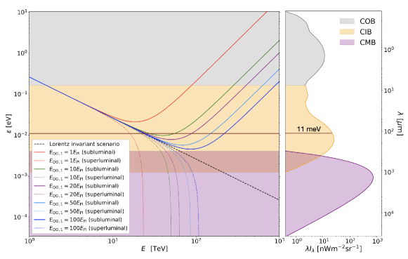
Figure 1: (Left) Energy of the background photons at threshold $(\epsilon_{\mathrm{th}})$ for the pair-production reaction as a function of a gamma-ray energy $(E)$. The black dashed line represents the Lorentz invariant scenario, while solid and doted lines represent LIV subluminal and superluminal scenarios, respectively. Five different values of $E_{\mathrm{EG,1}}$ were considered. (Right) Spectral energy distributions of the CMB and the two constituents of the EBL (cosmic optical background and cosmic infrared background) were produced using the EBL model by Domínguez et al. Domínguez et al. (2011).

The aforementioned Breit–Wheeler cross section, as a function of the gamma-ray energy, is shown in Figure 2. In the Lorentz invariant scenario, it is represented with a black dashed line. Once the reaction energy threshold is reached, the cross section rises quickly. At the gamma-ray energy roughly twice the threshold energy Madau and Phinney (1996), the Lorentz invariant cross section reaches its maximal value of $\simeq$$1.70\times 10^{-25}~{}\mathrm{cm}^{2}$ De Angelis et al. (2013). Afterwards, as the gamma-ray energy increases, the cross section drops and asymptotically approaches zero. In the superluminal scenario, the energy reaction threshold is lower than in the Lorentz invariant scenario. Moreover, lower $E_{\mathrm{QG,}1}$ results in lower reaction threshold. The cross section shape remains the same as in the Lorentz invariant scenario, although, it becomes narrower as $E_{\mathrm{QG,}1}$ decreases and reaches its maximum at lower gamma-ray energies. A somewhat more interesting development of the Breit–Wheeler cross section occurs in a subluminal LIV scenario. There are three distinct cases: (i) As we saw in Figure 1, for $E_{\mathrm{QG,}1}$ low enough, the reaction energy threshold will never be reached. Consequently, the cross section will be zero for all gamma-ray energies (red full line in the bottom panel of Figure 2). (ii) For higher values of $E_{\mathrm{QG,}1}$, the horizontal line will be crossed twice. Hence, there will be a lower and an upper reaction energy thresholds, and the reaction will be possible for gamma-ray energies between these thresholds. For relatively low $E_{\mathrm{QG,}1}$, this interval will be narrow, and the cross section will never reach its maximum possible value of $\simeq$$1.70\times 10^{-25}~{}\mathrm{cm}^{2}$ (green and violet full lines in the bottom panel of Figure 2). (iii) For even higher values of $E_{\mathrm{QG,}1}$, the gamma-ray energy interval between the reaction energy thresholds will be wide enough for the cross section to reach its maximum possible value. Moreover, the cross section will start to decrease with increasing gamma-ray energy, roughly following the shape of the Lorentz invariant cross section. However, as the gamma-ray energy rises, the cross section reaches a local minimum, and starts increasing to reach its maximum possible value once again, just below the upper reaction threshold. Once the threshold is reached, the cross section is cut off (light and dark blue full lines in the bottom panel of Figure 2). If one continued to increase the value of $E_{\mathrm{QG,}1}$, the second peak would become sharper and move towards higher energies, and the intermediate part of the cross section would more closely follow the Lorentz invariant cross section. In addition to these three cases, there are borderline cases. Between cases (i) and (ii), for $E_{\mathrm{QG,}1}$ precisely such that the horizontal line in Figure 1 is a tangent to the energy threshold line, the reaction energy threshold will be reached at precisely one gamma-ray energy, and the cross section will be a vertical line at that energy, and zero elsewhere. Between cases (ii) and (iii), the cross section would reach its maximum possible value, and monotonically drop to zero.

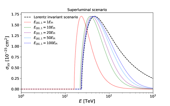
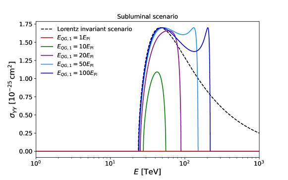
Figure 2: The Breit–Wheeler cross section as a function of the gamma-ray energy for the background photon energy of 11 meV and a head-on collision. The same five values of $E_{\mathrm{EG,1}}$ as in Figure 1 were considered. (Top) The black dashed line represents the Lorentz invariant scenario while doted lines represent LIV superluminal scenario. (Bottom) The black dashed line represents the Lorentz invariant scenario while full lines represent LIV subluminal scenario.

After seeing how modifications of photon dispersion relation influence the reaction energy threshold and the cross section, now it is time to see how the optical depth changes due to those modifications, since all experimental limits on $E_{\mathrm{QG}}$, based on the universe transparency, were set only for the subluminal scenario, we will focus only on this scenario. In Figure 3 we depicted a hypothetical gamma-ray absorption for a source at redshift $z_{\mathrm{s}}=0.03$ and gamma-ray energies up to 100 TeV, assuming different values of $E_{\mathrm{QG,1}}$. In the top panel of Figure 3 the gamma-ray horizon is denoted with a maroon line. As previously mentioned, beyond the gamma-ray horizon the universe becomes increasingly opaque for VHE gamma rays and thus the probability of their detection is diminishing. In the Lorentz invariant scenario, once the gamma-ray horizon is reached, the optical depth only increases. On the other hand, in the subluminal LIV scenario, the optical depth has a global maximum, different for different energies depending on the value of $E_{\mathrm{QG}}$, after which it decreases again. At some point it goes below the gamma-ray horizon allowing the gamma rays to evade absorption, which would lead to the recovery of the photon flux. The higher the $E_{\mathrm{QG}}$ scale, the higher the energy of the gamma-ray at which the recovery would occur. The absorption coefficient $(e^{-\tau})$, as a function of a gamma-ray energy $(E)$ is depicted in the bottom panel of Figure 3 and shows how the survival probability of the photons behaves in this scenario.

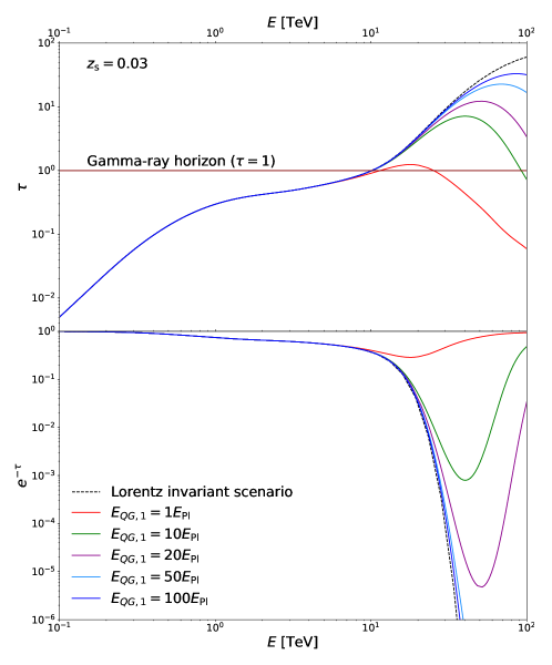
Figure 3: (Top) Optical depth $(\tau)$ as a function of a gamma-ray energy $(E)$ for a hypothetical source at $z_{\mathrm{s}}=0.03$. The black dashed line represents the Lorentz invariant scenario, while solid lines represent LIV subluminal scenario. Five different values of $E_{\mathrm{EG,1}}$ were considered. Gamma-ray horizon is denoted with the maroon line. (Bottom) The absorption coefficient $(e^{-\tau})$ as a function of a gamma-ray energy $(E)$.

It should be noted that there are other phenomena other than LIV which could leave imprints in the spectra of observed sources. Most notable are the axion-like particles, into which VHE gamma rays can oscillate in the presence of the external magnetic field. Nevertheless, imprints which axion-like particles and LIV would potentially leave could be mutually distinguished. Namely, axion-like particle imprints should be independent of the source redshift, while at the same time dependent on the magnetic field. The opposite holds for the LIV. For now, these two effects are being investigated separately, even in studies investigating both of them (see, e.g., Biteau and Williams (2015)). For more information about axion-like particles and their searches with IACT, we refer the interested reader to Batković et al. (2021); Abdalla et al. (2021).

3.1.2 Testing Lorentz Invariance Violation on Universe Transparency

The first experimental test of LIV on the EBL absorption of gamma rays using data from IACT was performed by Biteau $\&$ Williams Biteau and Williams (2015). The authors derived a simplified expression for optical depth using analytical methods. Furthermore, they constructed the EBL spectrum using 86 published gamma-ray spectra of 30 blazars with well-established redshifts. A total of $\sim$270,000 gamma rays constituted this gamma-ray sample. The EBL model was described through eight free parameters, denoted with $A$. In the LIV scenario, $E_{\mathrm{QG}}$ was added as one additional free parameter to the analysis, using the optical depth dependency on LIV described in the previous section. Furthermore, the EBL parameters were allowed to vary with $E_{\mathrm{QG}}$. In order to investigate the possible effects of LIV, Biteau $\&$ Williams compared spectra of the aforementioned blazars under the assumption of Lorentz invariance on the one hand, and under the assumption of LIV on the other hand. The effect of LIV was quantified using a test statistic (TS) defined as follows, with $\mathcal{L}=\exp(-TS/2)$:

$$TS=\chi^{2}\left(E_{\mathrm{QG}},A_{\mathrm{QG}}\right)-\chi^{2}\left(\infty,A_{\infty}\right).$$ (22)

The term $\chi^{2}\left(E_{\mathrm{QG}},A_{\mathrm{QG}}\right)$ represented the best fit in the LIV scenario. The $\chi^{2}\left(\infty,A_{\infty}\right)$ represented the best fit in the Lorentz invariant scenario since, as mentioned in Section 1.2, letting $E_{\mathrm{QG,1}}\rightarrow\infty$ leads to the Lorentz invariant photon dispersion relation.

Biteau $\&$ Williams adopted the formalism of Jacob and Piran (2008), which presumes that LIV affects both photons and leptons equally. Under that assumption, the last term in the energy threshold expression (Equation (21)) gains another factor of $(1-2^{-n})$. One of the 86 spectra selected for this study was the spectrum of Mrk 501 historical flare detected by HEGRA in 1997 Aharonian et al. (1999). When performing the analysis on the originally published Mrk 501 spectrum, Biteau $\&$ Williams showed that $E_{\mathrm{QG,1}}$ was approximately $E_{\mathrm{Pl}}$ at $4\sigma$ level. However, when a newly derived spectrum of the same data set (from Aharonian et al. (2001)) was used, the significance decreased to $2.4\,\sigma$. The re-analysed spectrum had better energy resolution, therefore it excluded the initially obtained highest energy data point. This example demonstrates how a single spectrum, and the most energetic photons in it, can greatly influence the final result. The first experimentally set $95\%$ confidence level lower limit, using universe transparency to VHE gamma rays, was found to be $E_{\mathrm{QG,1}}>9.5\times 10^{18}$ GeV. This value changed to $E_{\mathrm{QG,1}}>8.6\times 10^{18}$ GeV when a $10\%$ systematic uncertainty on the energy scale (typical for IACT) was accounted for.

3.1.3 The Most Constraining Limits Based on Single Source Analysis

Seventeen years after the historical flare from Mrk 501, which triggered discussions about the influence of LIV to universe’s transparency to VHE gamma rays, another bright flare brought Mrk 501 in the spotlight once again Cologna et al. (2017). This time it was used to constrain $E_{\mathrm{QG}}$ by the H.E.S.S. Collaboration using two independent channels Abdalla et al. (2019). The test of energy-dependent photon group velocity was described in Section 2.11, while the spectral analysis will be discussed here. Only the possible subluminal behaviour for linear or quadratic contributions was investigated. The pair production cross-section was calculated according to Fairbairn et al. (2014). In this approach, the modified expression for the square of the center of mass energy $s$ can be written as:

$$s=2E^{\prime}\epsilon^{\prime}(1-\cos\theta^{\prime})+S\left(\frac{E^{\prime}}{E_{\mathrm{QG,}n}}\right)^{n}E^{\prime 2}$$ (23)

The dependence of the cross section on $s$ is considered to be the same in LIV and Lorentz invariant scenarios. The cross section as a function of a gamma-ray energy for the background photon of 11 meV and a head-on collision is depicted in Figure 2.

To quantify the possible effects of LIV on a spectra of this bright flare, authors defined a TS similar to Equation (22):

$$\mathrm{TS}=\chi^{2}\left(E_{\mathrm{QG}}\right)-\chi^{2}\left(E_{\mathrm{QG}}\rightarrow\infty\right).$$ (24)

However, unlike the TS defined in Equation (22), this TS did not contain free-varying EBL parameters. The EBL model of Franceschini et al. Franceschini et al. (2008) was used and the optical depth was calculated in a standard way, as described in Equation (18). The $\chi^{2}$ values in Equation (24) were obtained by varying $E_{\mathrm{QG}}$ logarithmically and fitting the measured spectrum of a flare by an assumed intrinsic spectrum convoluted with the EBL attenuation effect. The intrinsic spectrum was assumed to be a simple power law. From the TS profiles, lower limits on $\mathrm{E}_{\mathrm{QG}}$ at $95\%$ confidence level were set to $E_{\mathrm{QG},1}>2.6\times 10^{19}$ GeV and $E_{\mathrm{QG},2}>7.8\times 10^{11}$ GeV for the linear and quadratic contributions, respectively.

A peculiarity of this work lies in the fact that the same data set was used to put the constraints on $E_{\mathrm{QG}}$ via energy-dependent time delay and the universe transparency effects, which we will discuss in more detail in Section 4.

3.1.4 On How the Most Constraining Limits Were Obtained

At the moment of writing this review, the best lower limits on $E_{\mathrm{QG}}$ obtained by testing the universe transparency were obtained by Lang et al. Lang et al. (2019). The starting data sample consisted of 111 spectra from 38 different sources available in the online catalogue TeVCat, of which only a subset was used for setting constraints on LIV. In order to select only the relevant sources for probing LIV, the authors defined the attenuation $a(E,z)$ as the ratio between the measured $J_{\text{meas}}(E)$ and the intrinsic $J_{\text{int}}(E,z)$ spectra of each source:

$$a(E,z)=e^{-\tau(E,z)}=\frac{J_{\text{meas}}(E)}{J_{\text{int}}(E,z)}$$ (25)

Lang et al. calculated the ratio between the attenuation assuming LIV and the attenuation in the Lorentz invariant scenario, at the maximum energy $(E_{\mathrm{max}})$ measured in a given spectrum. Only 18 spectra from 6 different sources for which the $a_{LIV}/a_{LI}$ ratio differed by at least $10\%$ and which could be used to further constrain $E_{\mathrm{QG}}$ were selected for further analysis.

In general, the intrinsic spectrum is obtained via the process of so-called deabsorption which consists in reverting the Equation (17). In previous studies, deabsorption was done under the assumption of Lorentz invariance, not taking into account LIV in this step of the analysis. In order to rectify it, Lang et al. used an energy interval which they call fiducial region. It is defined as the energy range starting at the lowest measured spectral point. The highest spectral point is the last one at which the difference between the fluxes assuming LIV and assuming Lorentz invariance are indistinguishable, considering the measurement uncertainties. Therefore only measured spectral points from bins that satisfy the following condition were used to determine the intrinsic spectrum:

$$\frac{a_{\mathrm{LIV}}}{a_{\mathrm{LI}}}\leq\frac{J_{\text{meas}}(E)+\rho\sigma\left(J_{\text{meas }}(E)\right)}{J_{\text{meas}}(E)}$$ (26)

Throughout their work, the authors assumed $\rho=1$, implying the tightest energy interval and hence leading to the most conservative limits on $E_{\mathrm{QG}}$. Every intrinsic spectrum $(J_{\mathrm{int}})$ was modeled as a power law with an exponential cut off. For each selected spectrum $(J_{\mathrm{int}})$, the energy spectrum on Earth $(J_{\mathrm{cal}})$ was computed for multiple $E_{\mathrm{QG,}n}$ values using

$$J_{\mathrm{cal}}=a_{\mathrm{LIV}}\times J_{\mathrm{int}}$$ (27)

Subsequently, all computed spectra were compared with the complete measured spectra $J_{\mathrm{meas}}$ using a log-likelihood method. Finally, the authors combined the likelihood results from all the sources to achieve the best possible sensitivity.

In their work, Lang et al. report $2\sigma$ confidence level lower limits on $E_{\mathrm{QG}}$ obtained with three different EBL models, using the same procedure. The most conservative limits were derived using the EBL model by Domínguez et al. Domínguez et al. (2011) and were set to be $E_{\mathrm{QG,1}}>6.85\times 10^{19}$ GeV and $E_{\mathrm{QG,2}}>1.56\times 10^{12}$ GeV.

3.2 Constraints on Violation of Lorentz Invariance from Atmospheric Showers Initiated by Multi-TeV Photons

The imaging technique of Cherenkov telescopes relies on recording flashes of Cherenkov light produced in the atmosphere by ultrarelativistic particles constituting extensive air showers. When a VHE gamma ray enters the Earth’s atmosphere, it is absorbed in the Coulomb field of an atomic nucleus in the air, creating an electron–positron pair. Each created particle carries approximately one half of the primary gamma ray’s energy. Leptons are emitting additional gamma rays through bremsstrahlung, each of which again go through the process of pair production. In that way, an electromagnetic cascade is created. The pair-creation is, fundamentally, the same process as the gamma-gamma interaction in which VHE gamma rays get absorbed by the EBL. Therefore, if the gamma-gamma interaction was affected by modifying the photon dispersion relation, it would also influence the development of particle showers in the atmosphere. This interesting notion was proposed by Rubtsov, Satunin & Sibiryakov in Rubtsov et al. (2014) and tested on data from HEGRA and H.E.S.S. in Rubtsov et al. (2017).

A shower development is governed by the Bethe–Heitler (B-H) process. In particular, the depth of the first interaction in the atmosphere is exponentially distributed with the mean value inversely proportional to the cross section Bethe and Heitler (1934)

$$\sigma_{\mathrm{BH}}=\frac{28Z^{2}\alpha^{3}\hbar^{2}c^{2}}{9m_{\mathrm{e}}^{2}c^{4}}\left(\log\frac{183}{Z^{1/3}}-\frac{1}{42}\right).$$ (28)

Here $Z$ is the atomic number of the nucleus, $\alpha$ is the fine structure constant, and $m_{\mathrm{e}}$ is the electron mass. In LIV scenario, the cross section will not change significantly for superluminal photons, unless the threshold for photon decay is reached. However, in that case, the photon decay will be the dominant process, making the LIV influence on the B-H process negligible. On the other hand, if photons are subluminal, the B-H cross section becomes strongly suppressed, leading to the suppression factor

$$\frac{\sigma_{\mathrm{BH}}^{\mathrm{LIV}}}{\sigma_{\mathrm{BH}}}\simeq\frac{12m_{\mathrm{e}}^{2}c^{4}E_{\mathrm{QG,2}}^{2}}{7E_{\gamma}^{4}}\log\frac{E_{\gamma}^{4}}{2m_{\mathrm{e}}^{2}c^{4}E_{\mathrm{QG,2}}^{2}}$$ (29)

As a consequence, the shower development in the LIV scenario will be impeded. The first gamma-gamma interaction will occur deeper in the atmosphere, and the effect will be more pronounced for higher gamma-ray energies. This will lead to showers reaching their maximal sizes also deeper in the atmosphere. Height of the shower maximum is an important parameter in IACT data analysis (see, e.g., de Naurois and Rolland (2009)). Depending on the experimental setup and the details of the data analysis, changes in the B-H cross section might lead to the showers induced by the most energetic gamma rays being misrepresented and excluded from further analysis. Ultimately, this will result in an apparent cut off in the spectrum at the high end.

Rubtsov, Satunin & Sibiryakov applied this method on two independent measurements of the Crab nebula spectrum. The first one was obtained by the HEGRA Collaboration, based on 385 h of observations performed between 1997 and 2002 Aharonian et al. (2004). The highest energy bin in the spectrum was centered at 75 GeV. The analysis method used to compare the spectra in Lorentz invariant versus LIV scenarios, and to determine limits to the LIV energy scale was based on ML method similar to the one used in Abdalla et al. (2019). They set a limit to the LIV energy scale to $E_{\mathrm{QG,2}}>2.1\times 10^{11}$ GeV. The second sample was the Crab nebula spectrum measured by the H.E.S.S. Collaboration, based on 4.4 h during the flaring episode in March 2013 Abramowski et al. (2014). In this case, the spectrum was determine up to $\sim$$40$ TeV. Because of the smaller data set and lower energies reached, the result was less constraining: $E_{\mathrm{QG,2}}>1.3\times 10^{11}$ GeV.

Note that this effect would be opposite to the one caused by modified absorption of gamma rays on the EBL (described in Section 3.1). The constraints on the LIV energy scale set in the work by Rubtsov, Satunin & Sibiryakov were lower than the ones obtained based on the universe transparency to gamma rays. However, the constraints based on the universe transparency were obtained assuming that shower development, and consequently measurement with IACT, is not modified by LIV. The work by Rubtsov, Satunin & Sibiryakov tested and validated that assumption.

3.3 Constraints on Lorentz Invariance Violation Based on Photon Stability

A modifying term in the photon dispersion relation can be treated as the mass term in the (unmodified) dispersion relation of a massive particle. Assigning a photon a mass in the superluminal scenario renders it unstable and prone to decay. A superluminal photon of energy $E_{\gamma}$ can:

• decay into an electron–positron pair

  $$\gamma\longrightarrow e^{+}+e^{-}.$$

  This reaction becomes possible under condition Martínez-Huerta and Pérez-Lorenzana (2017)

  $$E_{\mathrm{QG,}n}>E_{\gamma}\left(\frac{E_{\gamma}^{2}}{4m_{\mathrm{e}}^{2}c^{4}}-1\right)^{1/n},$$ (30)

  where $m_{\mathrm{e}}$ is the electron mass.
  

• split into multiple photons

  $$\gamma\longrightarrow N\gamma,$$

  with the dominant channel being splitting into three photons Astapov et al. (2019).

While the photon splitting has no reaction threshold, and is kinematically allowed for every superluminal photon, the process rate (see Astapov et al. (2019)) is significantly smaller than the photon decay rate Martínez-Huerta and Pérez-Lorenzana (2017); Albert et al. (2020).

Both processes have a similar effect on the observed spectra from astronomical sources, i.e., spectra will be attenuated at higher energies. Since there is no reaction threshold for the photon splitting, the attenuation will happen gradually. The photon decay rate quickly increases with the gamma-ray energy once the reaction threshold is reached. Consequently, it will be manifested as a cut off in the spectrum. The effects are similar to spectral attenuation due to gamma-ray absorption on the EBL. Therefore, in order to test for photon decay or photon splitting, one needs to exclude the possibility of EBL absorption. An obvious choice of a VHE gamma-ray source for these studies is the Crab nebula. Its spectrum reaches energies well above 100 TeV Amenomori et al. (2019); Abeysekara et al. (2019), while at the same time, because of its small distance from the Earth, EBL absorption is virtually negligible. These effects were independently tested for on Crab nebula spectral measurements in several studies (see, e.g., Martínez-Huerta and Pérez-Lorenzana (2017); Astapov et al. (2019); Satunin (2019)), however, the results setting substantially stronger constraints came not from any IACT experiment, but from the HAWC Collaboration Albert et al. (2020). The photon decay was used to constrain both liner and quadratic terms, obtaining $E_{\mathrm{QG,1}}>2.2\times 10^{22}$ GeV and $E_{\mathrm{QG,2}}>0.8\times 10^{14}$ GeV, respectively. The photon splitting was used only for the quadratic term, resulting in a much stronger constraint than the photon decay, $E_{\mathrm{QG,2}}>1.0\times 10^{15}$ GeV. Sheer moments before concluding this review, a very exciting result was published by LHAASO, announcing a detection of gamma rays with energies up to 1.4 PeV from 12 sources Cao et al. (2021). Based on these measurements the LHAASO Collaboration performed a similar study as HAWC. They searched for a cut of in spectra of the two sources with the highest energies LHAASO J0534+2202 (Crab nebula) and LHAASO J2032+4102 (the source which the 1.4 PeV event was associated with) Cao et al. (2021). Due to significantly higher spectral measurements by LHAASO, the resulting constraints on the LIV energy scale were also higher. Specifically, their most constraining limits were based on the analysis of LHAASO J2032+4102 spectrum. After including the systematic uncertainties, the limits were set to $E_{\mathrm{QG,1}}>1.2\times 10^{24}$ GeV and $E_{\mathrm{QG,2}}>1.1\times 10^{15}$ GeV, when the photon decay was considered. As in the HAWC analysis, only quadratic term was constrained based on photon splitting, resulting in $E_{\mathrm{QG,2}}>2.0\times 10^{16}$ GeV.

The scope of this review are studies performed with IACT. Nevertheless, we included these results from other type of observatories for comparison purposes. In addition, similar studies could be performed with IACT. With the prospect of the CTA to be commissioned in the next few years, and a recent result from the MAGIC Collaboration measuring the Crab nebula spectrum up to 100 TeV Acciari et al. (2020), feasibility of a similar study with IACT does not seem so far-fetched.

4 Summary and Discussion

In this section we will review and compare the results presented in previous sections. The results are summarised and listed chronologically in Table 4. A quick glance already reveals that the constraints, both on linear and quadratic terms, are the strongest in the case of the photon stability measurements Albert et al. (2020) by LHAASO, surpassing the Planck energy by four orders of magnitude in the case of the linear term. Apparently, that is the effect the most sensitive to LIV. However, as already stated in Section 3.3, photon decay and photon splitting are processes only allowed in superluminal scenario, and cannot be used to constrain $E_{\mathrm{QG}}$ in the subluminal scenario. Nevertheless, it was important to constrain this LIV effect. Possible photon decay and photon splitting competes with modified absorption of gamma rays on EBL. Without a confirmation of the photon stability to these substantially high values of $E_{\mathrm{QG}}$, it would be virtually impossible to resolve and independently search for LIV effects of modified universe transparency to gamma rays. As it happens, the second most constraining bounds were set precisely on measurements of the universe transparency for gamma rays, or gamma-gamma interaction. The most notable result was obtained by Lang et al. Lang et al. (2019) through a simultaneous analysis of spectra of several AGN. As already argued, combining different sources, should wash out dependence on the properties of a given source and, therefore, help to lift the degeneracy between the LIV and source intrinsic effects. The main characteristics of a desirable source for this method are large source distance and the highest spectral energy measurement. Combining various sources in a single study enables the most pronounced characteristic of each source to be fully exploited. However, the method heavily relies on the EBL modeling and the assumptions made on the intrinsic source spectra. Uncertainties of EBL models, as well as discrepancies between the different models, are the predominant source of systematic effects. Lang et al. considered this uncertainty by presenting the results of their analysis using three different EBL models. In this review, we presented the most conservative result.

Chronological census of bounds on the LIV energy scale as reported in the respective publications. The columns show from left to right: (i) LIV effect used to probe the QG, (ii) name of the observed source (when more than one source was used, we give the numner of the sources in the sample), (iii) type of the observed source, (iv) source redshift for extragalactic sources, and distance in kpc for sources in Milky Way, (v) analysis method used to perform the test, (vi) lower limit on the linear term in the modified photon dispersion relation, (vii) lower limit on the quadratic term in the modified photon dispersion relation, (viii) the experiment which produced the data sample, (ix) reference for the respective publication, (x) section in which the result was discussed in this work. Markers (+) and ($-$) in columns (vi) and (vii) represent superluminal and subluminal behaviours, respectively. The lower limits are expressed on the 95 % confidence level. Symbol ^† represents the best fit result in case where the estimated parameter was $>2\sigma$ away from Lorentz invariant scenario. Effect Source Type Distance Method $\bm{E_{\mathrm{QG,1}}}$ [GeV] $\bm{E_{\mathrm{QG,2}}}$ [GeV] Instr. Ref. Sec. Time delay Mrk 421 AGN $z=0.031$ band comparison $(-)\quad 0.4\times 10^{17}$ Whipple Biller et al. (1999) 2.1 Time delay Mrk 501 AGN $z=0.034$ ECF $(-)\quad 2.1\times 10^{17}$ $(-)\quad 2.6\times 10^{10}$ MAGIC MAGIC Collaboration et al. (2008) 2.2 Time delay Mrk 501 AGN $z=0.034$ ML $(-)\quad 3.0\times{10^{17}}^{~{}\dagger}$ $(-)\quad 5.7\times{10^{10}}~{}^{\dagger}$ MAGIC Martínez and Errando (2009) 2.4 Time delay PKS 2155-304 AGN $z=0.116$ MCCF $(-)\quad 7.2\times 10^{17}$ $(-)\quad 1.4\times 10^{9}$ H.E.S.S. Aharonian et al. (2008) 2.6 CWT $(-)\quad 5.2\times 10^{17}$ Time delay PKS 2155-304 AGN $z=0.116$ ML $(-)\quad 2.1\times 10^{18}$ $(-)\quad 6.4\times 10^{10}$ H.E.S.S. H. E. S. S. Collaboration et al. (2011) 2.6 Time delay GRB 090510 GRB $z=0.9$ PV, SMM, $(-)\quad 2.2\times 10^{19}$ $(-)\quad 4.0\times 10^{10}$ LAT Vasileiou et al. (2013) 2.13 and ML $(+)\quad 3.9\times 10^{19}$ $(+)\quad 3.0\times 10^{10}$ Time delay Crab Pulsar $d=2$ kpc PC $(-)\quad 3.0\times 10^{17}$ $(-)\quad 7.0\times 10^{9}$ VERITAS Otte (2011) 2.8 DisCan $(-)\quad 1.9\times 10^{17}$ Zitzer and VERITAS Collaboration (2013) $(+)\quad 1.7\times 10^{17}$ Time delay PG 1553+113 AGN $z=0.49$ ML $(-)\quad 4.1\times 10^{17}$ $(-)\quad 2.1\times 10^{10}$ H.E.S.S. Abramowski et al. (2015) 2.7 $(+)\quad 2.8\times 10^{17}$ $(+)\quad 1.7\times 10^{10}$ Time delay Vela Pulsar $d=0.3$ kpc ML $(-)\quad 4.0\times 10^{15}$ H.E.S.S. Chrétien et al. (2015) 2.10 $(+)\quad 3.7\times 10^{15}$ Universe transparency Multiple (30) AGN $z=0.019-0.287$ TS $(-)\quad 8.6\times 10^{18}$ Multiple Biteau and Williams (2015) 3.1.2 Bethe–Heitler Crab Nebula $d=2$ kpc ML $(-)\quad 2.1\times 10^{11}$ HEGRA Rubtsov et al. (2017) 3.2 $(-)\quad 1.3\times 10^{11}$ H.E.S.S. Time delay Crab Pulsar $d=2$ kpc PC $(-)\quad 1.1\times 10^{17}$ $(-)\quad 1.4\times 10^{10}$ MAGIC Ahnen et al. (2017) 2.9 $(+)\quad 1.1\times 10^{17}$ $(+)\quad 1.5\times 10^{10}$ ML $(-)\quad 5.5\times 10^{17}$ $(-)\quad 5.9\times 10^{10}$ $(+)\quad 4.5\times 10^{17}$ $(+)\quad 5.3\times 10^{10}$ Time delay Mrk 501 AGN $z=0.034$ ML $(-)\quad 3.6\times 10^{17}$ $(-)\quad 8.5\times 10^{10}$ H.E.S.S. Abdalla et al. (2019) 2.11 $(+)\quad 2.6\times 10^{17}$ $(+)\quad 7.3\times 10^{10}$ Universe transparency TS $(-)\quad 2.6\times 10^{19}$ $(-)\quad 7.8\times 10^{11}$ 3.1.3 Universe transparency Multiple (6) AGN $z=0.031-0.188$ TS $(-)\quad 6.9\times 10^{19}$ $(-)\quad 1.6\times 10^{12}$ Multiple Lang et al. (2019) 3.1.4 Photon decay Multiple (4) Galactic $d=1.55-2.37$ kpc TS $(+)\quad 2.2\times 10^{22}$ $(+)\quad 0.8\times 10^{14}$ HAWC Albert et al. (2020) 3.3 Photon splitting $(+)\quad 1.0\times 10^{15}$ Time delay GRB 190114C GRB $z=0.4245$ ML $(-)\quad 5.8\times 10^{18}$ $(-)\quad 6.3\times 10^{10}$ MAGIC Acciari et al. (2020) 2.12 $(+)\quad 5.5\times 10^{18}$ $(+)\quad 5.6\times 10^{10}$ Photon decay J2032+4102 Stellar $d=1.4$ kpc TS $(+)\quad 1.2\times 10^{24}$ $(+)\quad 1.1\times 10^{15}$ LHAASO Cao et al. (2021) 3.3 Photon splitting cluster $(+)\quad 2.0\times 10^{16}$

A second look at the Table 4 clearly shows that analyses based on photon interactions result in stronger constraints on $E_{\mathrm{QG}}$ compared to the ones based on photon time of flight. A study by the H.E.S.S. Collaboration was the only one so far in which both tests were performed on the same data set Abdalla et al. (2019). Granted, the two analyses were performed independently, the time of flight test ignoring modified gamma-ray absorption and vice versa. Nevertheless, it allowed a more direct comparison of the two effects of LIV. The constraints based on absorption of gamma rays on the EBL were more stringent by one order of magnitude on the quadratic term, and two orders of magnitude on the linear term, compared to the constraints based on energy-dependent time delay. Apart from the source distance and the detected energy, when it comes to time delay studies, another important property comes into play. Indeed, fast variability of flux is crucial in constraining emission times of individual photons (see Table 2.5). It should be noted that, while changes in flux do not strongly interfere with analysis based on EBL absorption, it is extremely important that the spectrum remains constant. A change in the spectrum would introduce additional uncertainties and hence lower the analysis sensitivity. Therefore, one may argue that a faster flux variability is needed to increase the sensitivity of time of flight tests. However, even the most sensitive of the time of flight analyses (Vasileiou et al. (2013) for the linear, and Abdalla et al. (2019) for the quadratic term) are below the sensitivities of analyses based on photon interactions, suggesting that (assuming the same $E_{\mathrm{QG}}$) LIV affects interactions more strongly than it does the photon group velocity. So, is there a point in testing energy-dependent photon group velocity, when we were able to set much stronger bounds on $E_{\mathrm{QG}}$ through tests of modified photon interactions? As we pointed out in Section 1.2, the theory of QG has not been formulated yet. Consequently, we do not know what the effects of QG are. It is quite possible that the photon group velocity is affected by the LIV, while interactions remain unaffected, or the other way around. Another possibility is that both interactions and propagation are affected, but on different scales, effectively introducing separate and different values of $E_{\mathrm{QG}}$. It should be remembered that the modified dispersion relation (Equation (1)) is merely a mathematical model facilitating experimental tests of LIV, and, in the most general case, different values of $E_{\mathrm{QG}}$ are applicable in different cases. Yet another imaginable scenario is that both subluminal and superluminal behaviours occur as different effects of QG. In that case, they might start to manifest at different energy scales, resulting in an even more complex expression for the photon group velocity (Equation (2)).

Considering the time delay studies alone, we observe a gradual increase of the lower limits on $E_{\mathrm{QG}}$. Of course, a study declaring a stricter limit (or a detection for that matter) is more likely to be published, however we would like to argue that this improvement is a result of several circumstances: (i) improvement on the performances of detectors allowed observations of sources at larger redshifts with better sampling, (ii) longer operations increased the probability of observing transient phenomena as flaring AGN and GRBs, as well as increased statistics on observations of pulsars, and (iii) analysis techniques, the ML in particular, have been refined over time, allowing for higher analysis sensitivity. A notable exception is the result obtained on the observation of GRB 090510 with Fermi-LAT. Published in 2013, the study by Vasileiou et al. Vasileiou et al. (2013) still holds the record for the most stringent bound on $E_{\mathrm{QG,1}}$. Let us analyse where this sensitivity came from. As conveyed in Table 2.5, the sensitivity of time of flight analyses increases with the energy of the gamma rays within the sample ($E_{\mathrm{max}}$) and the redshift of the source ($z_{\mathrm{s}}$), and decreases with the timescale of flux variations ($t_{\mathrm{var}}$). GRB 090510 has the second and third criterion well satisfied. The data set used in the analysis was taken from a time interval of less than 5 s (see Figure 1 in Vasileiou et al. (2013)), significantly shorter than any other sample covered in this review. At the same time, the redshift of $\sim$$0.9$ is more than two times larger than the second furthest source considered in Table 4. Apparently, the downside of the low highest energy in the sample (31 GeV) is more than well compensated by these two advantageous characteristics. In the case of the quadratic term, the relationship between $E_{\mathrm{max}}$, $t_{\mathrm{var}}$, and $z_{\mathrm{s}}$ is somewhat different. $E_{\mathrm{QG}}$ is still inversely proportional to the variability timescale, however $t_{\mathrm{var}}$ now enters through a square root, decreasing its influence on the analysis sensitivity. Furthermore, $E_{\mathrm{QG}}$ depends on the source redshift as $z_{\mathrm{s}}^{\sim 2/3}$ (in contrast to $z_{\mathrm{s}}^{\sim 1}$ in case of the linear term). Given that all sources are at redshifts smaller than 1, the influence of redshift is weaker on the quadratic term. Weaker influences of variability and redshift make more room for the influence of $E_{\mathrm{max}}$. Now, the tables have turned. The bound on $E_{\mathrm{QG,1}}$ set using MAGIC observation of GRB 190114C Acciari et al. (2020) was only about a factor 4 (7) below the limit from GRB 090510 for the subluminal (superluminal) behaviour. In the quadratic term, the influence of the highest gamma-ray energy is more pronounced than in the linear term. So, the constraint on $E_{\mathrm{QG,2}}$ became more stringent because of $\lesssim$$2$ TeV photons in the GRB 190114C sample. Actually, regarding the quadratic case, the strongest constraint came from the H.E.S.S. analysis of AGN Mrk 501, due to $\sim$$20$ TeV photons in the sample Abdalla et al. (2019).

Emission time from pulsars is excellently constrained, with the variability timescales down to $t_{\mathrm{var}}$$\sim$$10$ ms. Furthermore, gamma rays from pulses are detected up to $\sim$$7$ TeV. Unfortunately, their relatively close proximity renders LIV analyses on pulsars comparatively less sensitive, in particular in the linear scenario. On the other hand, in the quadratic scenario, their fast variability gives them a huge advantage, making them competitive sources for the search of LIV effect. Nonetheless, contrary to flaring AGN or GRBs, new observations of pulsar such as the Crab one do not depend on luck but can be carefully planned. This continuous accumulation of new data can lead to a predictable increase of statistics and therefore improved sensitivity of the analysis. This is particularly interesting as the current ML analyses are still mainly limited by background fluctuations and systematics such as the pulse shape and its energy evolution in the case of the Crab pulsar. In Ahnen et al. (2017) the authors stated that a total dataset of $\sim$$2000$ h on the Crab pulsar is within reach for the MAGIC collaboration alone given the regular observations performed for calibration purposes. And this data set could be further enlarged by taking into account the data accumulated on the Crab pulsar by H.E.S.S. and VERITAS (see also Section 5.2) with the potential of addressing some of the main limitations of the current analyses mentioned above and thus exploring QG scales beyond the current best limits, in particular in the quadratic scenario. Lastly, only pulsars with periods of a few tens of milliseconds have been detected with IACT so far. Detection of VHE gamma rays from pulsars with periods down to a few milliseconds would allow to constrain the emission time more strongly. This would lead to an improvement of the current limits on $E_{\mathrm{QG}}$ by an order of magnitude, further exploiting the potential of these sources in the search for LIV.

5 An Eye on the Future

In previous sections, we discussed the evolution of the search for LIV effects with IACT. The studies, which we reported on, have set strong constraints on the LIV energy scale, and significantly restricted the parameter space. More importantly, in those works, diverse ideas were proposed, various analysis methods had been developed, and different effects investigated. Ever since the first LIV study with an IACT, numerous ameliorations have been brought to the field in the form of technical or analysis improvements and the future ahead of us is certainly no exception. The most important question at this point is where do we go from here. What can we do to accelerate the research and contribute to the understanding of QG? In this section we try to outline some ideas on what could be the next steps in that regard. Hopefully, this will motivate the reader to perform some of the proposed research. We certainly intend to take our part in this endeavour.

5.1 Refinement of the Analysis Technique

In Section 2.3 we presented the state of the art ML method for testing energy-dependent photon group velocity. Here, we will discuss some possibilities for improving the method and increasing the analysis sensitivity.

Firstly, let us return to the definition of the likelihood function (Equation (10)) and in particular how individual events are selected and weighted. Note that the probability for each event to be a part of the signal, as defined in Equation (12), is the same for every event. The same is true for the probability for being a part of the background. Moreover, in order to reduce the background, the IACT data analysis involves applying cuts on the parameters describing events properties. This approach inevitably leads to cutting out some of the signal events as well. As we have seen, most of the LIV analysis methods rely on individual events. Therefore, cutting out signal events reduces the analysis sensitivity. However, in a recent paper, D’Amico et al. D’Amico et al. (2021) proposed an alternative IACT data analysis method, which considers all events in the ON region without applying any cut. Instead, PDFs for the signal and the background are calculated based on the parameters of individual events. This method could, therefore, be used to calculate $p^{(\mathrm{s})}_{i}$ and $p^{(\mathrm{b})}_{i}$ as PDFs, without discarding any events, whether of signal or background origin.

Secondly, the real strength of the ML method relies in its modularity, meaning that the components of the likelihood function listed in Section 2.3 can be refined, and additional terms describing nuisance parameters can be added without limitations. Furthermore, likelihoods from individual targets can easily be combined in a joint likelihood (see Section 5.2). For example, in case the intrinsic spectrum changes with time, the function $\Phi_{\mathrm{int}}(E)$ can be generalised to $\Phi_{\mathrm{int}}(E,t)$. Additionally, by taking the product $F(t+\eta_{n}E^{n})\Phi_{\mathrm{int}}(E)$ in Equation (11) we assumed that the emission time $t$ of individual photons does not depend on their energy. Indeed, in the LIV studies performed so far, there was no strong evidence of changes of spectral shape during AGN flaring episodes nor in GRBs in the VHE gamma-ray range. Nevertheless, waving this simplification might increase the sensitivity of the ML analyses. Present day state of the art models used to describe emission from astrophysical sources are nowhere near refined and accurate enough to predict the exact emission time of each particular photon. Hopefully, future emission models will be precise enough to allow creating emission light curve templates simultaneously depending on emission time and energy. E.g., instead of having independent temporal and spectral distributions as $F(t+\eta_{n}E^{n})\,\Phi_{\mathrm{int}}(E)$, we could take a two-dimensional distribution as $F_{\mathrm{2D}}(t+\eta_{n}E^{n},E)$ to account for potential source intrinsic delays. Therefore, further progress in the modelling of the sources emission mechanism such as initiated in Perennes et al. (2020) will certainly play an important role in future LIV studies.

5.2 Combining Data from Different Sources and Instruments

We have already seen on the example of the gamma-ray absorption (see Sections 3.1.2–3.1.4) how a combination of several sources in a single study improved the sensitivity of the analyses. An equivalent approach is still to be fully applied when testing the photon group velocity. Indeed, a combination of sources observed at a wide range of redshifts is the key to disentangling of intrinsic source effects from a real LIV effect. A source-intrinsic energy-dependent photon emission time can mimic an effect of LIV, leading to a misinterpretation as energy-dependent time of flight. Alternatively, intrinsic effects could have the same magnitude in the opposite direction from the LIV effect, canceling it and preventing a detection; a scenario known as a conspiracy of nature. Nonetheless, a LIV effect, if it exists, should be present in all observational data, and directly depend on the distance of a source. A combination of sources at different redshifts would mitigate the potential effect of source intrinsic effects. Furthermore, emission from different types of sources is a result of different physical processes, and subject to different emission dynamics. Therefore, combining different types of sources could further limit the contribution of source-intrinsic effects. These two factors, combining data from different types of sources and from observations at different redshifts, are instrumental in the development of a significantly more robust LIV analysis.

The likelihood function, can be relatively easily extended to consider additional data sets from the same or other sources. Note that a joint likelihood can be constructed from the product of individual likelihoods, each of them described by Equation (10). This single analysis of multiple data sets (sharing the same LIV parameter $\eta_{n}$) is possible as long as each data set is accompanied by its set of functions (light curve template, spectral distribution, acceptance, energy resolution, etc.) describing its particularity and its condition of observations.

Recently, an inter-experiment collaboration has been formed. The so-called LIV Consortium assembles researchers from all three currently operating IACT experiments (MAGIC, H.E.S.S., VERITAS) with the goal of combining data from different sources. In addition, the LIV Consortium is working on unifying observational data from different IACT facilities. This will immediately give access to a notably larger pool of sources than what has been used so far in LIV studies with IACT. Furthermore, combining different instruments in a single analysis, with a particular consideration of individual instrument response functions, is expected to decrease systematic uncertainties. Finally, such combination effort provides the necessary environment to harmonize the details of the analysis. As we have previously seen, analysis techniques can slightly differ from one experiment to the other. Combining individual best practices will further contribute to the research efficiency. Therefore, a combination of observations from all three currently operating IACT will provide a major improvement in the constraints on the LIV energy scale, not specifically on the facial value of the limits, but more importantly on the robustness of the results. The work done by the LIV Consortium can also be regarded as preparatory activities for the CTA era, which we discuss in the following paragraph. Preliminary results have been presented in conferences Nogués et al. (2017), while the final results are expected soon.

Another improvement in the direction of combining instruments would be to extend data samples to lower and higher energies, e.g., Fermi-LAT for the MeV–GeV energy range and HAWC or LHAASO for energies above PeV. These experiments provide complementary information to the one of IACT. It thus makes sense to combine the observations from these experiments to further increase the sensitivity of tests of LIV on gamma rays. Possible benefits are quite tantalizing, although such endeavor would be far from trivial, especially when it comes to treatment of different instrumental effects.

However, near future holds the prospect of the CTA, which will be an order of magnitude more sensitive than any of the existing Cherenkov telescopes CTA . Combined with a large number of telescopes, located in both hemispheres, the CTA will cover larger portions of the sky and observe more sources. This is particularly noteworthy for transient events, such as GRBs and AGN flares, and less bright sources, such as pulsars, all of which are essential for LIV studies. So far, only one LIV study was performed on a GRB observed with an IACT, and only a total of four GRBs have been observed with IACT until now. The CTA is expected to improve on this statistics. In Section 2.13, we discussed how Vasileiou et al. considered four GRBs in their study. GRB 090510, although located at the lowest redshift, yielded constraints on $E_{\mathrm{QG}}$ stronger by a factor of $2\text{--}20$ in the linear and $3\text{--}15$ in the quadratic scenarios, compared to results from other three GRBs Vasileiou et al. (2013). This was achieved due to a combination of the highest energy in the sample and the fastest variability. In Section 4 we compared the results obtained on GRB 090510 to the ones from GRB 190114C. The first one was a short GRB, with more than double the redshift of the second one. The signal from GRB 190114C was detected at two orders of magnitude higher energies, however the MAGIC telescopes detected mostly the afterglow phase. With the CTA, we hope to detect prompt emission as well, which is expected to be a more variable phase of GRBs. Furthermore, the CTA will extend the range of accessible energies both to lower (down to 20 GeV) and higher bands (up to 300 TeV). The highest energies detectable with the CTA will be almost an order of magnitude higher than the the ones accessible with the currently operating IACT. On the other hand, extending the observation window to lower energies, will grant access to gamma rays not absorbed by the EBL, enabling observations of sources at higher redshifts. Referring again to Table 2.5, higher redshift of a source improves the sensitivity to the LIV energy scale proportionally to the redshift in the linear, and somewhat less in the quadratic contribution. Alas, these two improvements cannot be combined. Gamma rays with the highest energies, emitted from the highest redshifts, will be absorbed by EBL before reaching Earth, so only one of these advantages will be accessible at a time. Nevertheless, there is an improvement coming from the wide energy range itself. Whichever effect of LIV is tested for (time of flight, universe transparency, etc.), the flux at the highest energies is compared to what is assumed to be the intrinsic emission. The latter is estimated from observations in the lower energy bands. LIV, if real, affects the gamma rays in the lower energy band as well the most energetic events. Granted, the effect is smaller for low energy band, but still present. Assuming that low energy photons are unaffected by the LIV induces a bias, and, ultimately, decreases the sensitivity of analyses. The bias will be smaller for a wider gap between the two energy bands used. Observations in the lower energy band can be obtained either using the same instrument, as in the case of e.g., PKS 2155-304 (see H. E. S. S. Collaboration et al. (2011) and Section 2.6), or from other instruments combined with theoretical inferences, as in the case of GRB 190114C (see Acciari et al. (2020) and Section 2.12). Ideally, observations in both energy bands would be performed with the same instrument with a wide range of observable energies. The former would reduce possible systematic effects, while the latter would decrease the potential LIV-induced bias. The CTA, with the range of accessible energies spanning over more than four orders of magnitude, will answer this need. While it is difficult to predict the light curves and spectra that the CTA will observe from GRBs, we can draw some conclusions by extrapolating the case of GRB 090510 to higher energies. Assuming that gamma rays emitted during the GRBs prompt phases can reach energies as high as few hundred GeV to a few TeV, the sensitivity to LIV effects would increase by one to two orders of magnitude. Even if we have to settle with lower redshifts, thus somewhat reducing the sensitivity (see Table 2.5; e.g., for $z=0.3$ the loss of sensitivity is at most a factor of $\sim$$3$ compared to $z=0.9$, the redshift of GRB 090510), the gain would still be substantial. A similar reasoning can be applied to studies based on spectral analysis. By lowering the detection energy threshold, the intrinsic spectra will be more precisely determined at the lower energy end of spectra, leading to better spectral fitting, and thus decreasing the uncertainties on the LIV energy scale. The CTA Consortium has published a projection of the CTA’s capabilities for probing fundamental physics, including LIV Abdalla et al. (2021). The study was limited to universe transparency to gamma rays. The authors estimated that the CTA will be able to probe the LIV energy scale a factor of two to three higher than the most sensitive studies published so far, whether based on a single source, or combining several sources.

5.3 Additional and Alternative Lorentz Invariance Violation Effects and Related Phenomena

Apart from the numerous interesting studies described in the previous sections, there are still a plethora of LIV-induced effects and related phenomena which have not been studied with IACT data. We will briefly mention those here.

Firstly, the energy-dependent arrival time delay between two simultaneously emitted photons from the same source is calculated from Equations (3) and (4). These were derived taking a comoving trajectories of the photons and their respective energy-dependent velocities. As mentioned in Section 2, one could start the derivation from a modified general relativistic dispersion relation Pfeifer (2018), or by modifying spacetime translations with the photon dispersion relation Rosati et al. (2015), and obtain different results for the photon time of flight. It would be interesting to investigate the differences between these models on IACT data.

Secondly, all the tests of energy-dependent photon group velocity performed on IACT data were based on Equation (2), which is deterministic in the sense that it assumes that all photons of the same energy will propagate with the same group velocity. However, there are models which propose fluctuations of the photon group velocity as a consequence of fluctuations of the spacetime foam Ellis et al. (2000). This phenomenon, often referred to as stochastic LIV models photon group velocity as Vasileiou et al. (2015):

$$v_{\gamma}(E)=c+\delta v_{\gamma}(E),$$ (31)

where the velocity modification $\delta v_{\gamma}(E)$ is randomly distributed according to normal distribution with mean in zero, and a standard deviation given with:

$$\sigma_{n}(E)=c\frac{1+n}{2}\left(\frac{E}{E_{\mathrm{QG,}n}}\right)^{n}.$$ (32)

The stochastic LIV was tested on Fermi-LAT observation of GRB 090510 Vasileiou et al. (2015). Only linear term was constrained to $E_{\mathrm{QG,1}}>3.4\times 10^{19}$ GeV. So far, no similar study was performed on IACT observations. As pointed out by Bolmont in Bolmont (2016), distant pulsars with sharp pulsation peaks would be excellent probes of stochastic LIV.

A substantial portion of this work was dedicated to effects LIV has on photon interactions. An important process in astrophysical sources of gamma rays is (inverse) Compton scattering. Abdalla & Böttcher analysed a possible influence of LIV on Compton scattering in Abdalla and Böttcher (2018) and concluded that LIV signatures were expected to be important only for incoming gamma-ray energies above $\sim$$1$ PeV. While in light of the recent results from LHAASO (see Section 3.3) this effect might draw some attention, Abdalla & Böttcher also concluded that even in the superluminal LIV scenario, the Klein–Nishina cross section would still be strongly dominated by the Thomson cross section, while in the subluminal scenario, the Klein–Nishina cross section would be even more strongly suppressed. Overall conclusion was that an LIV modified Compton scattering was not likely to be relevant in realistic astrophysical situations.

We would also like to point out that all investigations of universe transparency for gamma rays were performed on photons of energies up to 100 TeV. Remembering again the LHAASO detection of a photon of $\gtrsim 1$ PeV, we are strongly encouraged to extend our test to higher gamma-ray energies. As we have demonstrated in Section 3.1, and in particular in Figure 1, this will extend the photon target field to the CMB, which is substantially more dense than any of the EBL components. Moreover, in Figure 2, we have shown how the shape of the Breit–Wheeler cross section deforms in LIV subluminal scenario. These deformations were not significant for gamma-rays up to $\sim$$100$ TeV, but might play an important role for higher gamma-ray energies.

As previously mentioned, a study done by the H.E.S.S. Collaboration Abdalla et al. (2019) is the only one in which time of flight and universe transparency tests were performed on the same data set (see Sections 2.11 and 3.1.3). However, these two effects were tested independently of each other. In fact, there has never been a study that combined two different LIV effects. We have argued in Section 4 why strong limits based on one LIV effect do not necessarily constrain other effects. For example, limits on $E_{\mathrm{QG}}$ based on the universe transparency do not apply to the photon group velocity. Excluding one effect does not automatically exclude all LIV effects. Nonetheless, considering VHE gamma rays from astrophysical sources, it seems natural to wonder what would be the net observational result if several LIV effects were present. Namely, in Equation (11), term $F(E)$ takes into account propagation effects, such as EBL absorption, but under the assumption that photon interactions were not LIV affected. A combined effect study would presume that both photon group velocity and photon interactions were affected by the LIV. Different effects could manifest on the same, or different energy scales. Since there is no fully formulated theory of QG, and we do not know what the effects of QG are, this test is well justified. Implementation of such a test could be realised by modifying terms in the signal PDF in Equation (11). This might present a significant challenge, especially a computational one when maximising the likelihood function, and in particular if an independent value of $E_{\mathrm{QG}}$ is associated to each considered LIV effect.

Finally, there are possible effects of LIV, which have not been mentioned earlier, such as vacuum birefringence, vacuum dispersion, and vacuum anisotropy Kostelecky and Mewes (2008). The vacuum birefringence implies that the polarization vector of a linearly polarized photon will rotate dependently on the energy of the photon. As a consequence, a linearly polarised signal from an astrophysical source will be depolarised by the time it reaches Earth. Therefore, measurements of polarisation degree in a signal would constrain the vacuum birefringence effect (see, e.g., refs. Kislat and Krawczynski (2017); Friedman et al. (2020) for studies performed on optical observations, and refs. Toma et al. (2012); Kostelecký and Mewes (2013); Gotz et al. (2014) for studies performed on hard X-ray – soft gamma-ray observations.). These results are substantially more constraining than the tests based on modified photon kinematics. The ratio of sensitivities of the birefringence tests and the time of flight tests, performed on the same data sample, is proportional to the energy of the photons in the sample, as discussed by Kostelecký & Mewes in Kostelecky and Mewes (2009). As they put it descriptively, in order to achieve sensitivity in the time of flight tests comparable to the birefringence tests, one would need to achieve the timing resolution on the order of the inverse frequency of the photons. Even if this was instrumentally feasible (which is not), the measurement precision would be spoiled by the inability to constrain the photon emission times. Unfortunately, the IACT detection technique does not allow for measurements of gamma-ray polarisation. Recently, a novel satellite-based gamma-ray detector was proposed, which would be capable of measuring polarisation De Angelis et al. (2017) of gamma rays in a lower energy band. Unfortunately, the proposal was not accepted, but there is hope it will be selected for some future space mission, or that a similar concept such as AMEGO will be realised. X-ray polarimetry will certainly gain with soon to be launched IXPE.

Given that IACT cannot measure the polarisation of gamma rays, a broad discussion of birefringence would be out of the scope of this work. Nevertheless, considering strong constraints on LIV based on birefringence tests, we should note that these do not render time of flight tests useless. Indeed, already from theoretical considerations it is clear that in some cases the energy-dependent photon group velocity does not imply vacuum birefringence Kostelecky and Mewes (2009) (see also Bolmont (2016) for a critical discussion). Therefore, strong limits on the vacuum birefringence do not necessarily constrain the energy dependence of the photon group velocity. Furthermore, while IACT are not convenient for tests on photon polarisation, one should keep in mind that, as remarked in Zitzer and VERITAS Collaboration (2013), vacuum anisotropy could be constrained by performing LIV tests on sources in different directions. Hence, we should not be satisfied with setting stronger and stronger constraints on the LIV energy scale only. We should also strive towards building a rich statistics of sources located at different directions, as well as at different redshifts, as we already argued. Again, the CTA is expected to considerably contribute in this respect.

6 Conclusions

Most of investigators agree that there is a fundamental, quantum description of gravity. Though not formulated yet, the theory of QG is expected to resolve what happens in extreme gravitational potentials, such as singularities within black holes predicted by the general theory of relativity, or early universe, but also to push us in the direction of formulating the next unification theory describing all interactions. The expected realm of QG is the Planck scale, far above the reach of any physical laboratories present today, or any experiment envisaged in the near future. Nevertheless, some investigators believe even VHE gamma rays from astrophysical sources would feel minuscule effects of QG. These effects, consequences of the so-called LIV, would manifest as the photon group velocity deviating from the Lorentz invariant speed of light $c$, or as modified photon interactions. Given the cosmological distances gamma rays cover to reach Earth, there is a hope that these effects would accumulate sufficiently enough to be detected with gamma-ray detectors.

In this review we presented all experimental tests of LIV performed with IACT. We followed the historical development of the field. However, in order not to create a confusion, we first covered tests of energy-dependent photon group velocity, and then tests of modified photon interactions. A strictly chronological overview of the results was given in Table 4. 24 years have past since the first proposal that gamma rays emitted from astrophysical objects could be used to search for effects of QG. In fact, the proposal singled out GRBs as gamma-ray sources to be used for these tests. Only two years later, the first study using IACT Whipple was published on data from a blazar Mrk 421. Meanwhile, twenty more years had to pass before we were able to test the LIV on GRB 190114C observed by MAGIC. So far, no significant violation of the Lorentz symmetry was detected. However, in the past 22 years since the first experimental result was published, quite strict bounds were set on the level of LIV. In particular, considering the linear term in modified photon dispersion relation (Equation (1)), the lower limit on $E_{\mathrm{QG,1}}$ has surpassed the Planck energy. This is especially true when photon interactions are considered. While the expected energy level of QG is indeed the Planck scale, there is no strictly defined interval for $E_{\mathrm{QG}}$, so the test will continue. When it comes to the quadratic term in Equation (1), there is still quite some parameter space of $E_{\mathrm{QG,2}}$ to be investigated, both considering the photon group velocity and photon interactions; and in Section 4 we discussed why it is important to test for all possible effects, as well as both for subluminal and superluminal scenarios.

We hope to have demonstrated that IACT played an important role in search for LIV and setting strong constraints on its energy scale. More importantly, we tried to argue that IACT still have much to say in this field, and that observations with these instruments will ultimately lead to either detecting LIV, or confirming that the universe remains Lorentz invariant up to trans-Planckian energies. In Section 5 we presented our vision of the future development of this field. It goes without saying that we have great expectations of future facilities. In particular, the CTA, which promises a detection of several GRBs each year. However, new instruments will not do on their own, and additional improvements and development of analysis techniques will be necessary. In addition, there are hypothesised phenomena (e.g., stochastic LIV) which have not been tested for yet. Obviously, there is quite some work cut out for us. Whether we detect some effect of LIV, or it turns out that the Lorentz symmetry is perfectly preserved, one thing is for sure: exciting times are ahead.

All authors contributed equally to the writing. All authors have read and agreed to the published version of the manuscript. T.T. and J.S. acknowledge funding from the University of Rijeka, project number 13.12.1.3.02. T.T. also acknowledges funding from the Croatian Science Foundation (HrZZ), project number IP-2016-06-9782. D.K. acknowledges funding from the European Union’s Horizon 2020 research and innovation programme under the Marie Skłodowska-Curie grant agreement No. 754510, from the ERDF under the Spanish Ministerio de Ciencia e Innovación (MICINN), grant PID2019-107847RB-C41, and from the CERCA program of the Generalitat de Catalunya.

Abbreviations

The following acronyms and abbreviations are used in this manuscript:

AGN

active galactic nucleus

B-H

Bethe–Heitler

CMB

cosmic microwave background

CTA

Cherenkov Telescope Array

C.U.

Crab units

CWT

continuous wavelet transform

DisCan

dispersion cancellation

DSR

Doubly Special Relativity

EBL

extragalactic background light

ECF

energy cost function

FACT

First G-APD Cherenkov Telescope

GRB

gamma-ray burst

GBM

Gamma-ray Burst Monitor

HAWC

High Altitude Water Cherenkov

HEGRA

High Energy Gamma Ray Astronomy

H.E.S.S.

High Energy Stereoscopic System

IACT

imaging atmospheric Cherenkov telescope

LAT

Large Area Telescope

LHAASO

Large High Altitude Air Shower Observatory

LIV

Lorentz invariance violation

MAGIC

Major Atmospheric Gamma Imaging Cherenkov

MCCF

modified cross correlation function

MD

minimal dispersion

ML

maximum likelihood

PC

peak comparison

PDF

probability distribution function

PV

PairView

RB

radio background

QG

Quantum Gravity

SMM

sharpness maximisation method

TS

test statistic

VERITAS

Very Energetic Radiation Imaging Telescope Array System

VHE

very high energy (100 GeV $<E<$ 100 TeV)

References yes

References

- Einstein (1916) Einstein, A. The Foundation of the General Theory of Relativity. Annalen Phys. 1916, 49, 769–822. doi:\changeurlcolorblack10.1002/andp.200590044.
- Rovelli and Smolin (1990) Rovelli, C.; Smolin, L. Loop Space Representation of Quantum General Relativity. Nucl. Phys. B 1990, 331, 80–152. doi:\changeurlcolorblack10.1016/0550-3213(90)90019-A.
- Rovelli (2007) Rovelli, C., Quantum gravity. In Philosophy of physics; Butterfield, J.; Earman, J., Eds.; 2007. doi:\changeurlcolorblack10.1016/B978-044451560-5/50015-4.
- Oriti (2001) Oriti, D. Space-time geometry from algebra: Spin foam models for nonperturbative quantum gravity. Rept. Prog. Phys. 2001, 64, 1703–1756, [arXiv:gr-qc/0106091]. doi:\changeurlcolorblack10.1088/0034-4885/64/12/203.
- Niedermaier and Reuter (2006) Niedermaier, M.; Reuter, M. The Asymptotic Safety Scenario in Quantum Gravity. Living Rev. Rel. 2006, 9, 5–173. doi:\changeurlcolorblack10.12942/lrr-2006-5.
- Ambjorn et al. (2012) Ambjorn, J.; Goerlich, A.; Jurkiewicz, J.; Loll, R. Nonperturbative Quantum Gravity. Phys. Rept. 2012, 519, 127–210, [arXiv:1203.3591]. doi:\changeurlcolorblack10.1016/j.physrep.2012.03.007.
- Horowitz (2005) Horowitz, G.T. Spacetime in string theory. New J. Phys. 2005, 7, 201, [arXiv:gr-qc/0410049]. doi:\changeurlcolorblack10.1088/1367-2630/7/1/201.
- Kostelecky and Samuel (1989) Kostelecky, V.A.; Samuel, S. Spontaneous Breaking of Lorentz Symmetry in String Theory. Phys. Rev. D 1989, 39, 683. doi:\changeurlcolorblack10.1103/PhysRevD.39.683.
- Gambini and Pullin (1999) Gambini, R.; Pullin, J. Nonstandard optics from quantum space-time. Phys. Rev. D 1999, 59, 124021, [arXiv:gr-qc/9809038]. doi:\changeurlcolorblack10.1103/PhysRevD.59.124021.
- Carroll et al. (2001) Carroll, S.M.; Harvey, J.A.; Kostelecky, V.A.; Lane, C.D.; Okamoto, T. Noncommutative field theory and Lorentz violation. Phys. Rev. Lett. 2001, 87, 141601, [arXiv:hep-th/0105082]. doi:\changeurlcolorblack10.1103/PhysRevLett.87.141601.
- Douglas and Nekrasov (2001) Douglas, M.R.; Nekrasov, N.A. Noncommutative field theory. Rev. Mod. Phys. 2001, 73, 977–1029, [arXiv:hep-th/0106048]. doi:\changeurlcolorblack10.1103/RevModPhys.73.977.
- Bird et al. (1995) Bird, D.J.; Corbato, S.C.; Dai, H.Y.; Elbert, J.W.; Green, K.D.; Huang, M.A.; Kieda, D.B.; Ko, S.; Larsen, C.G.; Loh, E.C.; et al. Detection of a cosmic ray with measured energy well beyond the expected spectral cutoff due to cosmic microwave radiation. Astrophys. J. 1995, 441, 144–150, [arXiv:astro-ph/9410067]. doi:\changeurlcolorblack10.1086/175344.
- Halzen et al. (1995) Halzen, F.; Vázquez, R.A.; Stanev, T.; Vankov, H.P. The highest energy cosmic ray. Astropart. Phys. 1995, 3, 151–156. doi:\changeurlcolorblack10.1016/0927-6505(94)00038-5.
- Aartsen et al. (2021) Aartsen, M.G.; Abbasi, R.; Ackermann, M.; Adams, J.; Aguilar, J.A.; Ahlers, M.; Ahrens, M.; Alispach, C.; Amin, N.M.; Andeen, K.; et al. Detection of a particle shower at the Glashow resonance with IceCube. Nature 2021, 591, 220–224. [Erratum: Nature 592, E11 (2021)], doi:\changeurlcolorblack10.1038/s41586-021-03256-1.
- Cao et al. (2021) Cao, Z.; Aharonian, F.A.; An, Q.; Axikegu.; Bai, L.X.; Bai, Y.X.; Bao, Y.W.; Bastieri, D.; Bi, X.J.; Bi, Y.J.; et al. Ultrahigh-energy photons up to 1.4 petaelectronvolts from 12 -ray Galactic sources. Nature 2021. doi:\changeurlcolorblack10.1038/s41586-021-03498-z.
- Costa et al. (1997) Costa, E.; Feroci, M.; Piro, L.; Soffitta, P.; Amati, L.; Cinti, M.N.; Frontera, F.; Zavattini, G.; Nicastro, L.; Palazzi, E.; et al. GRB 970508. IAU Circ. 1997, 6649, 1.
- Djorgovski et al. (1997) Djorgovski, S.G.; Metzger, M.R.; Kulkarni, S.R.; Odewahn, S.C.; Gal, R.R.; Pahre, M.A.; Frail, D.A.; Feroci, M.; Costa, E.; Palazzi, E. The optical counterpart to the -ray burst GRB970508. Nature 1997, 387, 876–878. doi:\changeurlcolorblack10.1038/43126.
- Metzger et al. (1997) Metzger, M.R.; Djorgovski, S.G.; Kulkarni, S.R.; Steidel, C.C.; Adelberger, K.L.; Frail, D.A.; Costa, E.; Frontera, F. Spectral constraints on the redshift of the optical counterpart to the -ray burst of 8 May 1997. Nature 1997, 387, 878–880. doi:\changeurlcolorblack10.1038/43132.
- Amelino-Camelia et al. (1998) Amelino-Camelia, G.; Ellis, J.R.; Mavromatos, N.E.; Nanopoulos, D.V.; Sarkar, S. Tests of quantum gravity from observations of gamma-ray bursts. Nature 1998, 393, 763–765, [arXiv:astro-ph/9712103]. doi:\changeurlcolorblack10.1038/31647.
- Calcagni (2017) Calcagni, G. Lorentz violations in multifractal spacetimes. Eur. Phys. J. C 2017, 77, 291, [arXiv:1603.03046]. doi:\changeurlcolorblack10.1140/epjc/s10052-017-4841-6.
- Colladay and Kostelecky (1998) Colladay, D.; Kostelecky, V.A. Lorentz violating extension of the standard model. Phys. Rev. D 1998, 58, 116002, [arXiv:hep-ph/9809521]. doi:\changeurlcolorblack10.1103/PhysRevD.58.116002.
- Carroll et al. (1990) Carroll, S.M.; Field, G.B.; Jackiw, R. Limits on a Lorentz and Parity Violating Modification of Electrodynamics. Phys. Rev. D 1990, 41, 1231. doi:\changeurlcolorblack10.1103/PhysRevD.41.1231.
- Kostelecky and Mewes (2001) Kostelecky, V.A.; Mewes, M. Cosmological constraints on Lorentz violation in electrodynamics. Phys. Rev. Lett. 2001, 87, 251304, [arXiv:hep-ph/0111026]. doi:\changeurlcolorblack10.1103/PhysRevLett.87.251304.
- Amelino-Camelia (2002) Amelino-Camelia, G. Doubly special relativity. Nature 2002, 418, 34–35, [arXiv:gr-qc/0207049]. doi:\changeurlcolorblack10.1038/418034a.
- Amelino-Camelia (2010) Amelino-Camelia, G. Doubly-Special Relativity: Facts, Myths and Some Key Open Issues. Symmetry 2010, 2, 230–271, [arXiv:1003.3942]. doi:\changeurlcolorblack10.3390/sym2010230.
- Jacob and Piran (2008) Jacob, U.; Piran, T. Lorentz-violation-induced arrival delays of cosmological particles. JCAP 2008, 01, 031, [arXiv:0712.2170]. doi:\changeurlcolorblack10.1088/1475-7516/2008/01/031.
- Pfeifer (2018) Pfeifer, C. Redshift and lateshift from homogeneous and isotropic modified dispersion relations. Phys. Lett. B 2018, 780, 246–250, [arXiv:1802.00058]. doi:\changeurlcolorblack10.1016/j.physletb.2018.03.017.
- Rosati et al. (2015) Rosati, G.; Amelino-Camelia, G.; Marciano, A.; Matassa, M. Planck-scale-modified dispersion relations in FRW spacetime. Phys. Rev. D 2015, 92, 124042, [arXiv:1507.02056]. doi:\changeurlcolorblack10.1103/PhysRevD.92.124042.
- Weekes et al. (1989) Weekes, T.C.; Cawley, M.F.; Fegan, D.J.; Gibbs, K.G.; Hillas, A.M.; Kowk, P.W.; Lamb, R.C.; Lewis, D.A.; Macomb, D.; Porter, N.A.; et al.. Observation of TeV gamma rays from the Crab nebula using the atmospheric Cerenkov imaging technique. Astrophys. J. 1989, 342, 379–395. doi:\changeurlcolorblack10.1086/167599.
- Punch et al. (1992) Punch, M.; Akerlof, C.W.; Cawley, M.F.; Chantell, M.; Fegan, D.J.; Fennell, S.; Gaidos, J.A.; Hagan, J.; Hillas, A.M.; Jiang, Y.; et al. Detection of TeV photons from the active galaxy Markarian 421. Nature 1992, 358, 477–478. doi:\changeurlcolorblack10.1038/358477a0.
- Gaidos et al. (1996) Gaidos, J.A.; Akerlof, C.W.; Biller, S.; Boyle, P.J.; Breslin, A.C.; Buckley, J.H.; Carter-Lewis, D.A.; Catanese, M.; Cawley, M.F.; Fegan, D.J.; et al. Extremely rapid bursts of TeV photons from the active galaxy Markarian 421. Nature 1996, 383, 319–320. doi:\changeurlcolorblack10.1038/383319a0.
- Biller et al. (1999) Biller, S.D.; Breslin, A.C.; Buckley, J.; Catanese, M.; Carson, M.; Carter-Lewis, D.A.; Cawley, M.F.; Fegan, D.J.; Finley, J.P.; Gaidos, J.A.; et al. Limits to Quantum Gravity Effects on Energy Dependence of the Speed of Light from Observations of TeV Flares in Active Galaxies. Phys. Rev. Lett. 1999, 83, 2108–2111, [arXiv:gr-qc/9810044]. doi:\changeurlcolorblack10.1103/PhysRevLett.83.2108.
- Aleksić et al. (2016a) Aleksić, J.; Ansoldi, S.; Antonelli, L.A.; Antoranz, P.; Babic, A.; Bangale, P.; Barceló, M.; Barrio, J.A.; Becerra González, J.; Bednarek, W.; et al. The major upgrade of the MAGIC telescopes, Part I: The hardware improvements and the commissioning of the system. Astroparticle Physics 2016, 72, 61–75, [arXiv:1409.6073]. doi:\changeurlcolorblack10.1016/j.astropartphys.2015.04.004.
- Aleksić et al. (2016b) Aleksić, J.; Ansoldi, S.; Antonelli, L.A.; Antoranz, P.; Babic, A.; Bangale, P.; Barceló, M.; Barrio, J.A.; Becerra González, J.; Bednarek, W.; et al. The major upgrade of the MAGIC telescopes, Part II: A performance study using observations of the Crab Nebula. Astroparticle Physics 2016, 72, 76–94, [arXiv:1409.5594]. doi:\changeurlcolorblack10.1016/j.astropartphys.2015.02.005.
- Albert et al. (2007) Albert, J.; Aliu, E.; Anderhub, H.; Antoranz, P.; Armada, A.; Baixeras, C.; Barrio, J.A.; Bartko, H.; Bastieri, D.; Becker, J.K.; et al. Variable VHE gamma-ray emission from Markarian 501. Astrophys. J. 2007, 669, 862–883, [arXiv:astro-ph/0702008]. doi:\changeurlcolorblack10.1086/521382.
- Jackson (1999) Jackson, J.D. Classical electrodynamics; Wiley: New York, 1999.
- MAGIC Collaboration et al. (2008) MAGIC Collaboration.; Albert, J.; Aliu, E.; Anderhub, H.; Antonelli, L.A.; Antoranz, P.; Backes, M.; Baixeras, C.; Barrio, J.A.; Bartko, H.; Bastieri, D.; et al. Probing quantum gravity using photons from a flare of the active galactic nucleus Markarian 501 observed by the MAGIC telescope. Physics Letters B 2008, 668, 253–257, [arXiv:0708.2889]. doi:\changeurlcolorblack10.1016/j.physletb.2008.08.053.
- Vasileiou et al. (2013) Vasileiou, V.; Jacholkowska, A.; Piron, F.; Bolmont, J.; Couturier, C.; Granot, J.; Stecker, F.W.; Cohen-Tanugi, J.; Longo, F. Constraints on Lorentz Invariance Violation from Fermi-Large Area Telescope Observations of Gamma-Ray Bursts. Phys. Rev. D 2013, 87, 122001, [arXiv:1305.3463]. doi:\changeurlcolorblack10.1103/PhysRevD.87.122001.
- Barres de Almeida and Daniel (2012) Barres de Almeida, U.; Daniel, M.K. A Simple Method to Test for Energy-Dependent Dispersion in High Energy Light-Curves of Astrophysical Sources. Astropart. Phys. 2012, 35, 850–860, [arXiv:1204.2205]. doi:\changeurlcolorblack10.1016/j.astropartphys.2012.03.011.
- Scargle et al. (2008) Scargle, J.D.; Norris, J.P.; Bonnell, J.T. An Algorithm for Detecting Quantum Gravity Photon Dispersion in Gamma-Ray Bursts: DisCan. Astrophys. J. 2008, 673, 972–980. doi:\changeurlcolorblack10.1086/524396.
- Ellis et al. (2008) Ellis, J.R.; Harries, N.; Meregaglia, A.; Rubbia, A.; Sakharov, A. Probes of Lorentz Violation in Neutrino Propagation. Phys. Rev. D 2008, 78, 033013, [arXiv:0805.0253]. doi:\changeurlcolorblack10.1103/PhysRevD.78.033013.
- Martínez and Errando (2009) Martínez, M.; Errando, M. A new approach to study energy-dependent arrival delays on photons from astrophysical sources. Astroparticle Physics 2009, 31, 226–232, [arXiv:0803.2120]. doi:\changeurlcolorblack10.1016/j.astropartphys.2009.01.005.
- Wilks (1938) Wilks, S. The Large-Sample Distribution of the Likelihood Ratio for Testing Composite Hypotheses. Annals Math. Statist. 1938, 9, 60–62. doi:\changeurlcolorblack10.1214/aoms/1177732360.
- Berge et al. (2007) Berge, D.; Funk, S.; Hinton, J. Background Modelling in Very-High-Energy gamma-ray Astronomy. Astron. Astrophys. 2007, 466, 1219–1229, [arXiv:astro-ph/0610959]. doi:\changeurlcolorblack10.1051/0004-6361:20066674.
- Perennes et al. (2020) Perennes, C.; Sol, H.; Bolmont, J. Modeling spectral lags in active galactic nucleus flares in the context of Lorentz invariance violation searches. Astron. Astrophys. 2020, 633, A143, [arXiv:1911.10377]. doi:\changeurlcolorblack10.1051/0004-6361/201936430.
- Aleksić et al. (2010) Aleksić, J.; Antonelli, L.A.; Antoranz, P.; Backes, M.; Baixeras, C.; Barrio, J.A.; Bastieri, D.; Becerra González, J.; Bednarek, W.; Berdyugin, A.; et al. Search for an extended VHE gamma-ray emission from Mrk 421 and Mrk 501 with the MAGIC Telescope. Astron. Astrophys. 2010, 524, A77, [arXiv:1004.1093]. doi:\changeurlcolorblack10.1051/0004-6361/201014747.
- Abramowski et al. (2014) Abramowski, A.; Aharonian, F.; Ait Benkhali, F.; Akhperjanian, A.G.; Angüner, E.; Anton, G.; Backes, M.; Balenderan, S.; Balzer, A.; Barnacka, A.; et al. Search for Extended \gamma-ray Emission around AGN with H.E.S.S. and Fermi-LAT. Astron. Astrophys. 2014, 562, A145, [arXiv:1401.2915]. doi:\changeurlcolorblack10.1051/0004-6361/201322510.
- Ackermann et al. (2018) Ackermann, M.; Ajello, M.; Baldini, L.; Ballet, J.; Barbiellini, G.; Bastieri, D.; Bellazzini, R.; Bissaldi, E.; Blandford, R.D.; Bloom, E.D.; et al. The Search for Spatial Extension in High-latitude Sources Detected by the Large Area Telescope. Astrophys. J. Suppl. 2018, 237, 32, [arXiv:1804.08035]. doi:\changeurlcolorblack10.3847/1538-4365/aacdf7.
- Batista and Saveliev (2021) Batista, R.A.; Saveliev, A. The Gamma-ray Window to Intergalactic Magnetism. Universe 2021, 7, 223, [arXiv:2105.12020]. doi:\changeurlcolorblack10.3390/universe7070223.
- Sitarek and Bednarek (2010a) Sitarek, J.; Bednarek, W. Gamma-rays from the IC pair cascade in the radiation field of an accretion disk: Application to CenA. Mon. Not. Roy. Astron. Soc. 2010, 401, 1983, [arXiv:0909.5057]. doi:\changeurlcolorblack10.1111/j.1365-2966.2009.15785.x.
- Sitarek and Bednarek (2010b) Sitarek, J.; Bednarek, W. Time dependent gamma-ray production in the anisotropic IC pair cascade initiated by electrons in active galaxies. Mon. Not. Roy. Astron. Soc. 2010, 409, 662, [arXiv:1004.0172]. doi:\changeurlcolorblack10.1111/j.1365-2966.2010.17330.x.
- Aliu et al. (2008) Aliu, E.; Anderhub, H.; Antonelli, L.A.; Antoranz, P.; Backes, M.; Baixeras, C.; Barrio, J.A.; Bartko, H.; Bastieri, D.; Becker, J.K.; et al. Observation of Pulsed -Rays Above 25 GeV from the Crab Pulsar with MAGIC. Science 2008, 322, 1221, [arXiv:0809.2998]. doi:\changeurlcolorblack10.1126/science.1164718.
- Abdalla et al. (2018) Abdalla, H.; Aharonian, F.; Ait Benkhali, F.; Angüner, E.O.; Arakawa, M.; Arcaro, C.; Armand, C.; Arrieta, M.; Backes, M.; Barnard, M.; et al. First Ground-based Measurement of Sub-20 GeV to 100 GeV -rays from the Vela Pulsar with H.E.S.S. II. Astron. Astrophys. 2018, 620, A66, [arXiv:1807.01302]. doi:\changeurlcolorblack10.1051/0004-6361/201732153.
- Acciari et al. (2020) Acciari, V.A.; Ansoldi, S.; Antonelli, L.A.; Arbet Engels, A.; Asano, K.; Baack, D.; Babić, A.; Baquero, A.; Barres de Almeida, U.; Barrio, J.A.; et al. Detection of the Geminga pulsar with MAGIC hints at a power-law tail emission beyond 15 GeV. Astron. Astrophys. 2020, 643, L14, [arXiv:2011.10412]. doi:\changeurlcolorblack10.1051/0004-6361/202039131.
- Spir-Jacob et al. (2020) Spir-Jacob, M.; Djannati-Ataï, A.; Mohrmann, L.; Giavitto, G.; Khelifi, B.; Rudak, B.; Venter, C.; Zanin, R. Detection of sub-100 GeV-ray pulsations fromPSR B170644 with H.E.S.S. PoS 2020, ICRC2019, 799. doi:\changeurlcolorblack10.22323/1.358.0799.
- Meegan et al. (2009) Meegan, C.; Lichti, G.; Bhat, P.N.; Bissaldi, E.; Briggs, M.S.; Connaughton, V.; Diehl, R.; Fishman, G.; Greiner, J.; Hoover, A.S.; et al. The Fermi Gamma-Ray Burst Monitor. Astrophys. J. 2009, 702, 791–804, [arXiv:0908.0450]. doi:\changeurlcolorblack10.1088/0004-637X/702/1/791.
- Atwood et al. (2009) Atwood, W.B.; Abdo, A.A.; Ackermann, M.; Althouse, W.; Anderson, B.; Axelsson, M.; Baldini, L.; Ballet, J.; Band, D.L.; Barbiellini, G.; et al. The Large Area Telescope on the Fermi Gamma-ray Space Telescope Mission. Astrophys. J. 2009, 697, 1071–1102, [arXiv:0902.1089]. doi:\changeurlcolorblack10.1088/0004-637X/697/2/1071.
- Bhat et al. (2016) Bhat, P.; Meegan, C.A.; von Kienlin, A.; Paciesas, W.S.; Briggs, M.S.; Burgess, J.M.; Burns, E.; Chaplin, V.; Cleveland, W.H.; Collazzi, A.C.; et al. The Third Fermi gbm Gamma-ray Burst Catalog: the First six Years. Astrophys. J. Suppl. 2016, 223, 28, [arXiv:1603.07612]. doi:\changeurlcolorblack10.3847/0067-0049/223/2/28.
- Acciari et al. (2019) Acciari, V.A.; Ansoldi, S.; Antonelli, L.A.; Arbet Engels, A.; Baack, D.; Babić, A.; Banerjee, B.; Barres de Almeida, U.; Barrio, J.A.; Becerra González, J.; et al. Teraelectronvolt emission from the -ray burst GRB 190114C. Nature 2019, 575, 455–458, [arXiv:2006.07249]. doi:\changeurlcolorblack10.1038/s41586-019-1750-x.
- Abdalla et al. (2019) Abdalla, H.; Adam, R.; Aharonian, F.; Ait Benkhali, F.; Angüner, E.O.; Arakawa, M.; Arcaro, C.; Armand, C.; Ashkar, H.; Backes, M.; et al. A very-high-energy component deep in the -ray burst afterglow. Nature 2019, 575, 464–467, [arXiv:1911.08961]. doi:\changeurlcolorblack10.1038/s41586-019-1743-9.
- de Naurois and H. E. S. S. Collaboration (2019) de Naurois, M.; H. E. S. S. Collaboration. GRB190829A: Detection of VHE gamma-ray emission with H.E.S.S. GRB Coordinates Network 2019, 25566, 1.
- Blanch et al. (2020) Blanch, O.; Longo, F.; Berti, A.; Fukami, S.; Suda, Y.; Loporchio, S.; Micanovic, S.; Green, J.G.; Pinter, V.; Takahashi, M.; MAGIC Collaboration. GRB 201216C: MAGIC detection in very high energy gamma rays. GRB Coordinates Network 2020, 29075, 1.
- Ashton et al. (2020) Ashton, T.; Backes, M.; Balzer, A.; Berge, D.; Bolmont, J.; Bonnefoy, S.; Brun, F.; Chaminade, T.; Delagnes, E.; Fontaine, G.; et al. A NECTAr-based upgrade for the Cherenkov cameras of the H.E.S.S. 12-meter telescopes. Astroparticle Physics 2020, 118, 102425, [arXiv:2001.04510]. doi:\changeurlcolorblack10.1016/j.astropartphys.2019.102425.
- Aharonian et al. (2007) Aharonian, F.; Akhperjanian, A.G.; Bazer-Bachi, A.R.; Behera, B.; Beilicke, M.; Benbow, W.; Berge, D.; Bernlöhr, K.; Boisson, C.; Bolz, O.; et al. An Exceptional Very High Energy Gamma-Ray Flare of PKS 2155-304. Astrophys. J. Lett. 2007, 664, L71–L78, [arXiv:0706.0797]. doi:\changeurlcolorblack10.1086/520635.
- Aharonian et al. (2008) Aharonian, F.; Akhperjanian, A.G.; Barres de Almeida, U.; Bazer-Bachi, A.R.; Becherini, Y.; Behera, B.; Beilicke, M.; Benbow, W.; Bernlöhr, K.; Boisson, C.; et al. Limits on an Energy Dependence of the Speed of Light from a Flare of the Active Galaxy PKS 2155-304. Phys. Rev. Lett. 2008, 101, 170402, [arXiv:0810.3475]. doi:\changeurlcolorblack10.1103/PhysRevLett.101.170402.
- Li et al. (2004) Li, T.P.; Qu, J.L.; Feng, H.; Song, L.M.; Ding, G.Q.; Chen, L. Timescale analysis of spectral lags. Chin. J. Astron. Astrophys. 2004, 4, 583–598, [arXiv:astro-ph/0407458]. doi:\changeurlcolorblack10.1088/1009-9271/4/6/583.
- H. E. S. S. Collaboration et al. (2011) H. E. S. S. Collaboration.; Abramowski, A.; Acero, F.; Aharonian, F.; Akhperjanian, A.G.; Anton, G.; Barnacka, A.; Barres de Almeida, U.; Bazer-Bachi, A.R.; Becherini, Y.; Becker, J.; et al. Search for Lorentz Invariance breaking with a likelihood fit of the PKS 2155-304 flare data taken on MJD 53944. Astroparticle Physics 2011, 34, 738–747, [arXiv:1101.3650]. doi:\changeurlcolorblack10.1016/j.astropartphys.2011.01.007.
- Abramowski et al. (2015) Abramowski, A.; Aharonian, F.; Ait Benkhali, F.; Akhperjanian, A.G.; Angüner, E.O.; Backes, M.; Balenderan, S.; Balzer, A.; Barnacka, A.; Becherini, Y.; et al. The 2012 flare of PG 1553+113 seen with H.E.S.S. and Fermi-LAT. Astrophys. J. 2015, 802, 65, [arXiv:1501.05087]. doi:\changeurlcolorblack10.1088/0004-637X/802/1/65.
- Kaaret (1999) Kaaret, P. Pulsar radiation and quantum gravity. Astron. Astrophys. 1999, 345, L32, [arXiv:astro-ph/9903464].
- Kaplan et al. (2008) Kaplan, D.L.; Chatterjee, S.; Gaensler, B.M.; Anderson, J. A Precise Proper Motion for the Crab Pulsar, and the Difficulty of Testing Spin-Kick Alignment for Young Neutron Stars. Astrophys. J. 2008, 677, 1201, [arXiv:0801.1142]. doi:\changeurlcolorblack10.1086/529026.
- Manchester et al. (2005) Manchester, R.N.; Hobbs, G.B.; Teoh, A.; Hobbs, M. The Australia Telescope National Facility pulsar catalogue. Astron. J. 2005, 129, 1993, [arXiv:astro-ph/0412641]. doi:\changeurlcolorblack10.1086/428488.
- VERITAS Collaboration et al. (2011) VERITAS Collaboration.; Aliu, E.; Arlen, T.; Aune, T.; Beilicke, M.; Benbow, W.; Bouvier, A.; Bradbury, S.M.; Buckley, J.H.; Bugaev, V.; Byrum, K.; et al. Detection of Pulsed Gamma Rays Above 100 GeV from the Crab Pulsar. Science 2011, 334, 69, [arXiv:1108.3797]. doi:\changeurlcolorblack10.1126/science.1208192.
- Otte (2011) Otte, N. Prospects of performing Lorentz invariance tests with VHE emission from Pulsars. International Cosmic Ray Conference, 2011, Vol. 7, International Cosmic Ray Conference, p. 256. doi:\changeurlcolorblack10.7529/ICRC2011/V07/1302.
- Zitzer and VERITAS Collaboration (2013) Zitzer, B.; VERITAS Collaboration. Lorentz Invariance Violation Limits from the Crab Pulsar using VERITAS. International Cosmic Ray Conference, 2013, Vol. 33, International Cosmic Ray Conference, p. 2768, [arXiv:1307.8382].
- Abdo et al. (2010) Abdo, A.A.; Ackermann, M.; Ajello, M.; Atwood, W.B.; Axelsson, M.; Baldini, L.; Ballet, J.; Barbiellini, G.; Baring, M.G.; Bastieri, D.; et al. Fermi Large Area Telescope Observations of the Crab Pulsar and Nebula. Astrophys. J. 2010, 708, 1254–1267, [arXiv:0911.2412]. doi:\changeurlcolorblack10.1088/0004-637X/708/2/1254.
- Buccheri et al. (1983) Buccheri, R.; Bennett, K.; Bignami, G.F.; Bloemen, J.B.G.M.; Boriakoff, V.; Caraveo, P.A.; Hermsen, W.; Kanbach, G.; Manchester, R.N.; Masnou, J.L.; et al. Search for pulsed gamma-ray emission from radio pulsars in the COS-B data. Astron. Astrophys. 1983, 128, 245–251.
- Ahnen et al. (2017) Ahnen, M.L.; Ansoldi, S.; Antonelli, L.A.; Arcaro, C.; Babić, A.; Banerjee, B.; Bangale, P.; Barres de Almeida, U.; Barrio, J.A.; Becerra González, J.; et al. Constraining Lorentz invariance violation using the Crab Pulsar emission observed up to TeV energies by MAGIC. Astrophys. J. Suppl. 2017, 232, 9, [arXiv:1709.00346]. doi:\changeurlcolorblack10.3847/1538-4365/aa8404.
- Caraveo et al. (2001) Caraveo, P.A.; De Luca, A.; Mignani, R.P.; Bignami, G.F. The distance to the vela pulsar gauged with hst parallax oservations. Astrophys. J. 2001, 561, 930, [arXiv:astro-ph/0107282]. doi:\changeurlcolorblack10.1086/323377.
- Chrétien et al. (2015) Chrétien, M.; Bolmont, J.; Jacholkowski, A. Constraining photon dispersion relation from observations of the Vela pulsar with H.E.S.S. 34th International Cosmic Ray Conference (ICRC2015), 2015, Vol. 34, International Cosmic Ray Conference, p. 764, [arXiv:1509.03545].
- Anderhub et al. (2013) Anderhub, H.; Backes, M.; Biland, A.; Boccone, V.; Braun, I.; Bretz, T.; Buß, J.; Cadoux, F.; Commichau, V.; Djambazov, L.; et al. Design and operation of FACT - the first G-APD Cherenkov telescope. Journal of Instrumentation 2013, 8, P06008, [arXiv:1304.1710]. doi:\changeurlcolorblack10.1088/1748-0221/8/06/P06008.
- Abdalla et al. (2019) Abdalla, H.; Aharonian, F.; Ait Benkhali, F.; Angüner, E.O.; Arakawa, M.; Arcaro, C.; Armand, C.; Arrieta, M.; Backes, M.; Barnard, M.; et al. The 2014 TeV -Ray Flare of Mrk 501 Seen with H.E.S.S.: Temporal and Spectral Constraints on Lorentz Invariance Violation. Astrophys. J. 2019, 870, 93, [arXiv:1901.05209]. doi:\changeurlcolorblack10.3847/1538-4357/aaf1c4.
- Mirzoyan et al. (2019) Mirzoyan, R.; Noda, K.; Moretti, E.; Berti, A.; Nigro, C.; Hoang, J.; Micanovic, S.; Takahashi, M.; Chai, Y.; Moralejo, A.; MAGIC Collaboration. MAGIC detects the GRB 190114C in the TeV energy domain. GRB Coordinates Network 2019, 23701, 1.
- Acciari et al. (2020) Acciari, V.A.; Ansoldi, S.; Antonelli, L.A.; Arbet Engels, A.; Baack, D.; Babić, A.; Banerjee, B.; Barres de Almeida, U.; Barrio, J.A.; Becerra González, J.; et al. Bounds on Lorentz invariance violation from MAGIC observation of GRB 190114C. Phys. Rev. Lett. 2020, 125, 021301, [arXiv:2001.09728]. doi:\changeurlcolorblack10.1103/PhysRevLett.125.021301.
- Acciari et al. (2019) Acciari, V.A.; Ansoldi, S.; Antonelli, L.A.; Arbet Engels, A.; Baack, D.; Babić, A.; Banerjee, B.; Barres de Almeida, U.; Barrio, J.A.; Becerra González, J.; et al. Observation of inverse Compton emission from a long -ray burst. Nature 2019, 575, 459–463, [arXiv:2006.07251]. doi:\changeurlcolorblack10.1038/s41586-019-1754-6.
- Hassan et al. (2017) Hassan, T.; Arrabito, L.; Bernlöhr, K.; Bregeon, J.; Cortina, J.; Cumani, P.; Di Pierro, F.; Falceta-Goncalves, D.; Lang, R.G.; Hinton, J.; et al. Monte Carlo Performance Studies for the Site Selection of the Cherenkov Telescope Array. Astropart. Phys. 2017, 93, 76–85, [arXiv:1705.01790]. doi:\changeurlcolorblack10.1016/j.astropartphys.2017.05.001.
- Inoue et al. (2013) Inoue, S.; Granot, J.; O’Brien, P.T.; Asano, K.; Bouvier, A.; Carosi, A.; Connaughton, V.; Garczarczyk, M.; Gilmore, R.; Hinton, J.; et al. Gamma-Ray Burst Science in the Era of the Cherenkov Telescope Array. Astropart. Phys. 2013, 43, 252–275, [arXiv:1301.3014]. doi:\changeurlcolorblack10.1016/j.astropartphys.2013.01.004.
- Greiner et al. (2009) Greiner, J.; Clemens, C.; Krühler, T.; von Kienlin, A.; Rau, A.; Sari, R.; Fox, D.B.; Kawai, N.; Afonso, P.; Ajello, M.; et al. The redshift and afterglow of the extremely energetic gamma-ray burst GRB 080916C. Astron. Astrophys. 2009, 498, 89–94, [arXiv:0902.0761]. doi:\changeurlcolorblack10.1051/0004-6361/200811571.
- Olivares et al. (2009) Olivares, F.; Klose, S.; Kruehler, T.; Greiner, J. GRB 090510: GROND observations. GRB Coordinates Network 2009, 9352, 1.
- Cucchiara et al. (2009) Cucchiara, A.; Fox, D.B.; Tanvir, N.; Berger, E. GRB 090902B: Gemini-N absorption redshift. GRB Coordinates Network 2009, 9873, 1.
- D’Elia et al. (2010) D’Elia, V.; Fynbo, J.P.U.; Covino, S.; Goldoni, P.; Jakobsson, P.; Matteucci, F.; Piranomonte, S.; Sollerman, J.; Thöne, C.C.; Vergani, S.D.; et al. VLT/X-shooter spectroscopy of the GRB 090926A afterglow. Astron. Astrophys. 2010, 523, A36, [arXiv:1007.5357]. doi:\changeurlcolorblack10.1051/0004-6361/201015216.
- (91) CTAO Performance. https://www.cta-observatory.org/science/ctao-performance/. Accessed July 15, 2021.
- Kifune (1999) Kifune, T. Invariance violation extends the cosmic ray horizon? Astrophys. J. Lett. 1999, 518, L21–L24, [arXiv:astro-ph/9904164]. doi:\changeurlcolorblack10.1086/312057.
- Aloisio et al. (2000) Aloisio, R.; Blasi, P.; Ghia, P.L.; Grillo, A.F. Probing the structure of space-time with cosmic rays. Phys. Rev. D 2000, 62, 053010, [arXiv:astro-ph/0001258]. doi:\changeurlcolorblack10.1103/PhysRevD.62.053010.
- Amelino-Camelia (2004) Amelino-Camelia, G. Phenomenology of Planck-scale Lorentz-symmetry test theories. New Journal of Physics 2004, 6, 188, [arXiv:gr-qc/0212002]. doi:\changeurlcolorblack10.1088/1367-2630/6/1/188.
- Gould and Schréder (1967) Gould, R.J.; Schréder, G.P. Pair Production in Photon-Photon Collisions. Phys. Rev. 1967, 155, 1404–1407. doi:\changeurlcolorblack10.1103/PhysRev.155.1404.
- Stecker et al. (1992) Stecker, F.W.; de Jager, O.C.; Salamon, M.H. TeV gamma rays from 3C 279 - A possible probe of origin and intergalactic infrared radiation fields. Astrophys. J. Lett. 1992, 390, L49. doi:\changeurlcolorblack10.1086/186369.
- Biteau and Williams (2015) Biteau, J.; Williams, D.A. The extragalactic background light, the Hubble constant, and anomalies: conclusions from 20 years of TeV gamma-ray observations. Astrophys. J. 2015, 812, 60, [arXiv:1502.04166]. doi:\changeurlcolorblack10.1088/0004-637X/812/1/60.
- Abdalla and Böttcher (2018) Abdalla, H.; Böttcher, M. Lorentz Invariance Violation Effects on Gamma–Gamma Absorption and Compton Scattering. Astrophys. J. 2018, 865, 159, [arXiv:1809.00477]. doi:\changeurlcolorblack10.3847/1538-4357/aadb87.
- Hauser and Dwek (2001) Hauser, M.G.; Dwek, E. The cosmic infrared background: measurements and implications. Ann. Rev. Astron. Astrophys. 2001, 39, 249–307, [arXiv:astro-ph/0105539]. doi:\changeurlcolorblack10.1146/annurev.astro.39.1.249.
- Franceschini (2021) Franceschini, A. Photon–Photon Interactions and the Opacity of the Universe in Gamma Rays. Universe 2021, 7, 146. doi:\changeurlcolorblack10.3390/universe7050146.
- Franceschini et al. (2008) Franceschini, A.; Rodighiero, G.; Vaccari, M. The extragalactic optical-infrared background radiations, their time evolution and the cosmic photon-photon opacity. Astron. Astrophys. 2008, 487, 837, [arXiv:0805.1841]. doi:\changeurlcolorblack10.1051/0004-6361:200809691.
- Domínguez et al. (2011) Domínguez, A.; Primack, J.R.; Rosario, D.J.; Prada, F.; Gilmore, R.C.; Faber, S.M.; Koo, D.C.; Somerville, R.S.; Pérez-Torres, M.A.; Pérez-González, P.; et al. Extragalactic Background Light Inferred from AEGIS Galaxy SED-type Fractions. Mon. Not. Roy. Astron. Soc. 2011, 410, 2556, [arXiv:1007.1459]. doi:\changeurlcolorblack10.1111/j.1365-2966.2010.17631.x.
- Gilmore et al. (2012) Gilmore, R.C.; Somerville, R.S.; Primack, J.R.; Dominguez, A. Semi-analytic modeling of the EBL and consequences for extragalactic gamma-ray spectra. Mon. Not. Roy. Astron. Soc. 2012, 422, 3189, [arXiv:1104.0671]. doi:\changeurlcolorblack10.1111/j.1365-2966.2012.20841.x.
- Abdalla et al. (2017) Abdalla, H.; Abramowski, A.; Aharonian, F.; Ait Benkhali, F.; Akhperjanian, A.G.; Andersson, T.; Angüner, E.O.; Arakawa, M.; Arrieta, M.; Aubert, P.; et al. Measurement of the EBL spectral energy distribution using the VHE -ray spectra of H.E.S.S. blazars. Astron. Astrophys. 2017, 606, A59, [arXiv:1707.06090]. doi:\changeurlcolorblack10.1051/0004-6361/201731200.
- Acciari et al. (2019) Acciari, V.A.; Ansoldi, S.; Antonelli, L.A.; Arbet Engels, A.; Baack, D.; Babić.; , A.; Banerjee, B.; Barres de Almeida, U.; Barrio, J.A.; Becerra González, J.; et al. Measurement of the extragalactic background light using MAGIC and Fermi-LAT gamma-ray observations of blazars up to z = 1. Mon. Not. Roy. Astron. Soc. 2019, 486, 4233–4251, [arXiv:1904.00134]. doi:\changeurlcolorblack10.1093/mnras/stz943.
- Abeysekara et al. (2019) Abeysekara, A.U.; Archer, A.; Benbow, W.; Bird, R.; Brill, A.; Brose, R.; Buchovecky, M.; Calderon-Madera, D.; Christiansen, J.L.; Cui, W.; et al. Measurement of the extragalactic background light spectral energy distribution with VERITAS 2019. [arXiv:1910.00451]. doi:\changeurlcolorblack10.3847/1538-4357/ab4817.
- Breit and Wheeler (1934) Breit, G.; Wheeler, J.A. Collision of Two Light Quanta. Physical Review 1934, 46, 1087–1091. doi:\changeurlcolorblack10.1103/PhysRev.46.1087.
- Blanch and Martinez (2005) Blanch, O.; Martinez, M. Exploring the gamma ray horizon with the next generation of gamma ray telescopes. Part 1: Theoretical predictions. Astroparticle Physics 2005, 23, 588–597, [arXiv:astro-ph/0107582]. doi:\changeurlcolorblack10.1016/j.astropartphys.2005.03.008.
- Aharonian et al. (1999) Aharonian, F.A.; Akhperjanian, A.G.; Barrio, J.A.; Bernlöhr, K.; Bojahr, H.; Calle, I.; Contreras, J.L.; Cortina, J.; Daum, A.; Deckers, T.; et al. The time averaged TeV energy spectrum of mkn 501 of the extraordinary 1997 outburst as measured with the stereoscopic Cherenkov telescope system of HEGRA. Astron. Astrophys. 1999, 349, 11–28, [arXiv:astro-ph/9903386].
- Pühlhofer et al. (2003) Pühlhofer, G.; Bolz, O.; Götting, N.; Heusler, A.; Horns, D.; Kohnle, A.; Lampeitl, H.; Panter, M.; Tluczykont, M.; Aharonian, F.; et al. The technical performance of the HEGRA system of imaging air Cherenkov telescopes. Astropart. Phys. 2003, 20, 267–291, [arXiv:astro-ph/0306123]. doi:\changeurlcolorblack10.1016/j.astropartphys.2003.06.001.
- Blanch et al. (2003) Blanch, O.; Lopez, J.; Martinez, M. Testing the effective scale of quantum gravity with the next generation of gamma ray telescopes. Astroparticle Physics 2003, 19, 245–252, [arXiv:astro-ph/0107334]. doi:\changeurlcolorblack10.1016/S0927-6505(02)00205-0.
- Jacobson et al. (2003) Jacobson, T.; Liberati, S.; Mattingly, D. A Strong astrophysical constraint on the violation of special relativity by quantum gravity. Nature 2003, 424, 1019–1021, [arXiv:astro-ph/0212190]. doi:\changeurlcolorblack10.1038/nature01882.
- Protheroe and Meyer (2000) Protheroe, R.J.; Meyer, H. An infrared background-TeV gamma-ray crisis? Physics Letters B 2000, 493, 1–6, [arXiv:astro-ph/0005349]. doi:\changeurlcolorblack10.1016/S0370-2693(00)01113-8.
- Amelino-Camelia and Piran (2001) Amelino-Camelia, G.; Piran, T. Planck scale deformation of Lorentz symmetry as a solution to the UHECR and the TeV gamma paradoxes. Phys. Rev. D 2001, 64, 036005, [arXiv:astro-ph/0008107]. doi:\changeurlcolorblack10.1103/PhysRevD.64.036005.
- Jacob and Piran (2008) Jacob, U.; Piran, T. Inspecting absorption in the spectra of extra-galactic gamma-ray sources for insight on Lorentz invariance violation. Phys. Rev. D 2008, 78, 124010, [arXiv:0810.1318]. doi:\changeurlcolorblack10.1103/PhysRevD.78.124010.
- Tavecchio and Bonnoli (2016) Tavecchio, F.; Bonnoli, G. On the detectability of Lorentz invariance violation through anomalies in the multi-TeV -ray spectra of blazars. Astron. Astrophys. 2016, 585, A25, [arXiv:1510.00980]. doi:\changeurlcolorblack10.1051/0004-6361/201526071.
- Madau and Phinney (1996) Madau, P.; Phinney, E.S. Constraints on the Extragalactic Background Light from Gamma-Ray Observations of High-Redshift Quasars. Astrophys. J. 1996, 456, 124. doi:\changeurlcolorblack10.1086/176633.
- De Angelis et al. (2013) De Angelis, A.; Galanti, G.; Roncadelli, M. Transparency of the Universe to gamma rays. Mon. Not. Roy. Astron. Soc. 2013, 432, 3245–3249, [arXiv:1302.6460]. doi:\changeurlcolorblack10.1093/mnras/stt684.
- Batković et al. (2021) Batković, I.; De Angelis, A.; Doro, M.; Manganaro, M. Axion-Like Particle Searches with IACTs. Universe 2021, 7, 185, [arXiv:2106.03424]. doi:\changeurlcolorblack10.3390/universe7060185.
- Abdalla et al. (2021) Abdalla, H.; Abe, H.; Acero, F.; Acharyya, A.; Adam, R.; Agudo, I.; Aguirre-Santaella, A.; Alfaro, R.; Alfaro, J.; Alispach, C.; et al. Sensitivity of the Cherenkov Telescope Array for probing cosmology and fundamental physics with gamma-ray propagation. JCAP 2021, 02, 048, [arXiv:2010.01349]. doi:\changeurlcolorblack10.1088/1475-7516/2021/02/048.
- Aharonian et al. (2001) Aharonian, F.A.; Akhperjanian, A.G.; Barrio, J.A.; Bernlöhr, K.; Bolz, O.; Börst, H.; Bojahr, H.; Contreras, J.L.; Cortina, J.; Denninghoff, S.; et al.. Reanalysis of the high energy cutoff of the 1997 mkn 501 TeV energy spectrum. Astron. Astrophys. 2001, 366, 62, [arXiv:astro-ph/0011483]. doi:\changeurlcolorblack10.1051/0004-6361:20000098.
- Cologna et al. (2017) Cologna, G.; Chakraborty, N.; Jacholkowska, A.; Lorentz, M.; Mohamed, M.; Perennes, C.; Romoli, C.; Wagner, S.J.; Wierzcholska, A.; H. E. S. S. Collaboration.; Dorner, D.; FACT Collaboration.; Kurtanidze, O. The Exceptional Flare of Mrk 501 in 2014: Combined Observations with H.E.S.S. and FACT. AIP Conf. Proc. 2017, 1792, 050019, [arXiv:1611.03983]. doi:\changeurlcolorblack10.1063/1.4968965.
- Fairbairn et al. (2014) Fairbairn, M.; Nilsson, A.; Ellis, J.; Hinton, J.; White, R. The CTA Sensitivity to Lorentz-Violating Effects on the Gamma-Ray Horizon. JCAP 2014, 06, 005, [arXiv:1401.8178]. doi:\changeurlcolorblack10.1088/1475-7516/2014/06/005.
- Lang et al. (2019) Lang, R.G.; Martínez-Huerta, H.; de Souza, V. Improved limits on Lorentz invariance violation from astrophysical gamma-ray sources. Phys. Rev. D 2019, 99, 043015, [arXiv:1810.13215]. doi:\changeurlcolorblack10.1103/PhysRevD.99.043015.
- Rubtsov et al. (2014) Rubtsov, G.; Satunin, P.; Sibiryakov, S. Prospective constraints on Lorentz violation from ultrahigh-energy photon detection. Phys. Rev. D 2014, 89, 123011, [arXiv:1312.4368]. doi:\changeurlcolorblack10.1103/PhysRevD.89.123011.
- Rubtsov et al. (2017) Rubtsov, G.; Satunin, P.; Sibiryakov, S. Constraints on violation of Lorentz invariance from atmospheric showers initiated by multi-TeV photons. JCAP 2017, 05, 049, [arXiv:1611.10125]. doi:\changeurlcolorblack10.1088/1475-7516/2017/05/049.
- Bethe and Heitler (1934) Bethe, H.; Heitler, W. On the Stopping of fast particles and on the creation of positive electrons. Proc. Roy. Soc. Lond. A 1934, 146, 83–112. doi:\changeurlcolorblack10.1098/rspa.1934.0140.
- de Naurois and Rolland (2009) de Naurois, M.; Rolland, L. A high performance likelihood reconstruction of gamma-rays for Imaging Atmospheric Cherenkov Telescopes. Astropart. Phys. 2009, 32, 231, [arXiv:0907.2610]. doi:\changeurlcolorblack10.1016/j.astropartphys.2009.09.001.
- Aharonian et al. (2004) Aharonian, F.; Akhperjanian, A.; Beilicke, M.; Bernlöhr, K.; Börst, H.G.; Bojahr, H.; Bolz, O.; Coarasa, T.; Contreras, J.L.; Cortina, J.; et al. The Crab nebula and pulsar between 500-GeV and 80-TeV. Observations with the HEGRA stereoscopic air Cerenkov telescopes. Astrophys. J. 2004, 614, 897–913, [arXiv:astro-ph/0407118]. doi:\changeurlcolorblack10.1086/423931.
- Abramowski et al. (2014) Abramowski, A.; Aharonian, F.; Ait Benkhali, F.; Akhperjanian, A.G.; Angüner, E.; Anton, G.; Balenderan, S.; Balzer, A.; Barnacka, A.; Becherini, Y.; et al. H.E.S.S. Observations of the Crab during its March 2013 GeV Gamma-Ray Flare. Astron. Astrophys. 2014, 562, L4, [arXiv:1311.3187]. doi:\changeurlcolorblack10.1051/0004-6361/201323013.
- Martínez-Huerta and Pérez-Lorenzana (2017) Martínez-Huerta, H.; Pérez-Lorenzana, A. Restrictions from Lorentz invariance violation on cosmic ray propagation. Phys. Rev. D 2017, 95, 063001, [arXiv:1610.00047]. doi:\changeurlcolorblack10.1103/PhysRevD.95.063001.
- Astapov et al. (2019) Astapov, K.; Kirpichnikov, D.; Satunin, P. Photon splitting constraint on Lorentz Invariance Violation from Crab Nebula spectrum. JCAP 2019, 04, 054, [arXiv:1903.08464]. doi:\changeurlcolorblack10.1088/1475-7516/2019/04/054.
- Albert et al. (2020) Albert, A.; Alfaro, R.; Alvarez, C.; Angeles Camacho, J.R.; Arteaga-Velázquez, J.C.; Arunbabu, K.P.; Avila Rojas, D.; Ayala Solares, H.A.; Baghmanyan, V.; Belmont-Moreno, E.; et al. Constraints on Lorentz Invariance Violation from HAWC Observations of Gamma Rays above 100 TeV. Phys. Rev. Lett. 2020, 124, 131101, [arXiv:1911.08070]. doi:\changeurlcolorblack10.1103/PhysRevLett.124.131101.
- Amenomori et al. (2019) Amenomori, M.; Bao, Y.W.; Bi, X.J.; Chen, D.; Chen, T.L.; Chen, W.Y.; Chen, X.; Chen, Y.; Cirennima.; Cui, S.W.; et al. First Detection of Photons with Energy beyond 100 TeV from an Astrophysical Source. Phys. Rev. Lett. 2019, 123, 051101, [arXiv:1906.05521]. doi:\changeurlcolorblack10.1103/PhysRevLett.123.051101.
- Abeysekara et al. (2019) Abeysekara, A.U.; Albert, A.; Alfaro, R.; Alvarez, C.; Álvarez, J.D.; Camacho, J.R.A.; Arceo, R.; Arteaga-Velázquez, J.C.; Arunbabu, K.P.; Avila Rojas, D.; et al. Measurement of the Crab Nebula at the Highest Energies with HAWC. Astrophys. J. 2019, 881, 134, [arXiv:1905.12518]. doi:\changeurlcolorblack10.3847/1538-4357/ab2f7d.
- Satunin (2019) Satunin, P. New constraints on Lorentz Invariance violation from Crab Nebula spectrum beyond TeV. Eur. Phys. J. C 2019, 79, 1011, [arXiv:1906.08221]. doi:\changeurlcolorblack10.1140/epjc/s10052-019-7520-y.
- Cao et al. (2019) Cao, Z.; Chen, M.J.; Chen, S.Z.; Hu, H.B.; Liu, C.; Liu, Y.; Ma, L.L.; Ma, X.H.; Sheng, X.D.; Wu, H.R.; et al. Introduction to Large High Altitude Air Shower Observatory (LHAASO). Chin. Astron. Astrophys. 2019, 43, 457–478. doi:\changeurlcolorblack10.1016/j.chinastron.2019.11.001.
- Cao et al. (2021) Cao, Z.; others. Exploring Lorentz Invariance Violation from Ultra-high-energy Gamma Rays Observed by LHAASO 2021. [arXiv:2106.12350].
- Acciari et al. (2020) Acciari, V.A.; Ansoldi, S.; Antonelli, L.A.; Arbet Engels, A.; Baack, D.; Babić, A.; Banerjee, B.; Barres de Almeida, U.; Barrio, J.A.; Becerra González, J.; et al. MAGIC very large zenith angle observations of the Crab Nebula up to 100 TeV. Astron. Astrophys. 2020, 635, A158, [arXiv:2001.09566]. doi:\changeurlcolorblack10.1051/0004-6361/201936899.
- D’Amico et al. (2021) D’Amico, G.; Terzić, T.; Strišković, J.; Doro, M.; Strzys, M.; van Scherpenberg, J. Signal estimation in on/off measurements including event-by-event variables. Phys. Rev. D 2021, 103, 123001, [arXiv:2105.01019]. doi:\changeurlcolorblack10.1103/PhysRevD.103.123001.
- Nogués et al. (2017) Nogués, L.; Lin, T.T.Y.; Perennes, C.; Gent, A.E.; Bolmont, J.; Gaug, M.; Jacholkowska, A.; Martinez, M.; Otte, A.N.; Wagner, R.; Ward, J.E.; Zitzer, B.; Consortium, L. First combined studies on Lorentz Invariance Violation from observations of astrophysical sources. 35th International Cosmic Ray Conference (ICRC2017), 2017, Vol. 301, International Cosmic Ray Conference, p. 646, [arXiv:1710.08342].
- Ellis et al. (2000) Ellis, J.R.; Mavromatos, N.E.; Nanopoulos, D.V. Quantum gravitational diffusion and stochastic fluctuations in the velocity of light. Gen. Rel. Grav. 2000, 32, 127–144, [arXiv:gr-qc/9904068]. doi:\changeurlcolorblack10.1023/A:1001852601248.
- Vasileiou et al. (2015) Vasileiou, V.; Granot, J.; Piran, T.; Amelino-Camelia, G. A Planck-scale limit on spacetime fuzziness and stochastic Lorentz invariance violation. Nature Phys. 2015, 11, 344–346. doi:\changeurlcolorblack10.1038/nphys3270.
- Bolmont (2016) Bolmont, J. Is the speed of light in vacuum really constant? Habilitation à diriger des recherches, UPMC, 2016.
- Kostelecky and Mewes (2008) Kostelecky, V.A.; Mewes, M. Astrophysical Tests of Lorentz and CPT Violation with Photons. Astrophys. J. Lett. 2008, 689, L1–L4, [arXiv:0809.2846]. doi:\changeurlcolorblack10.1086/595815.
- Kislat and Krawczynski (2017) Kislat, F.; Krawczynski, H. Planck-scale constraints on anisotropic Lorentz and CPT invariance violations from optical polarization measurements. Phys. Rev. D 2017, 95, 083013, [arXiv:1701.00437]. doi:\changeurlcolorblack10.1103/PhysRevD.95.083013.
- Friedman et al. (2020) Friedman, A.S.; Gerasimov, R.; Leon, D.; Stevens, W.; Tytler, D.; Keating, B.G.; Kislat, F. Improved constraints on anisotropic birefringent Lorentz invariance and violation from broadband optical polarimetry of high redshift galaxies. Phys. Rev. D 2020, 102, 043008, [arXiv:2003.00647]. doi:\changeurlcolorblack10.1103/PhysRevD.102.043008.
- Toma et al. (2012) Toma, K.; Mukohyama, S.; Yonetoku, D.; Murakami, T.; Gunji, S.; Mihara, T.; Morihara, Y.; Sakashita, T.; Takahashi, T.; Wakashima, Y.; et al. Strict Limit on CPT Violation from Polarization of Gamma-Ray Burst. Phys. Rev. Lett. 2012, 109, 241104, [arXiv:1208.5288]. doi:\changeurlcolorblack10.1103/PhysRevLett.109.241104.
- Kostelecký and Mewes (2013) Kostelecký, V.A.; Mewes, M. Constraints on relativity violations from gamma-ray bursts. Phys. Rev. Lett. 2013, 110, 201601, [arXiv:1301.5367]. doi:\changeurlcolorblack10.1103/PhysRevLett.110.201601.
- Gotz et al. (2014) Gotz, D.; Laurent, P.; Antier, S.; Covino, S.; D’Avanzo, P.; D’Elia, V.; Melandri, A. GRB 140206A: the most distant polarized Gamma-Ray Burst. Mon. Not. Roy. Astron. Soc. 2014, 444, 2776–2782, [arXiv:1408.4121]. doi:\changeurlcolorblack10.1093/mnras/stu1634.
- Kostelecky and Mewes (2009) Kostelecky, V.A.; Mewes, M. Electrodynamics with Lorentz-violating operators of arbitrary dimension. Phys. Rev. D 2009, 80, 015020, [arXiv:0905.0031]. doi:\changeurlcolorblack10.1103/PhysRevD.80.015020.
- De Angelis et al. (2017) De Angelis, A.; Tatischeff, V.; Tavani, M.; Oberlack, U.; Grenier, I.; Hanlon, L.; Walter, R.; Argan, A.; von Ballmoos, P.; Bulgarelli, A.; et al. The e-ASTROGAM mission. Exper. Astron. 2017, 44, 25–82, [arXiv:1611.02232]. doi:\changeurlcolorblack10.1007/s10686-017-9533-6.