Resonance frequency of different interfacial modes and steady streaming by a slug trapped at one end of a millichannel

Abstract

Active micropumping and micromixing using oscillating bubbles form the basis for various Lab-on-chip applications. Acoustically excited oscillatory bubbles are also used in active particle sorting, ultrasonic imaging, cell lysis and rotation. For efficient micromixing, the system must be operated at its resonant frequency where amplitude of oscillation is maximum. This ensures that high-intensity cavitation microstreaming is generated. In this work, we determine the resonant frequencies for the different surface modes of oscillation of a rectangular gas slug confined at one end of a millichannel using perturbation techniques and matched asymptotic expansions. We explicitly specify the oscillation frequency of the interface and compute the surface mode amplitudes from the interface deformation. This oscillatory flow field at the leading order is also determined. The effect of aspect ratio of gas slug on observable streaming is analysed. The predictions of surface modes from perturbation theory are validated with simulations of the system done in ANSYS Fluent.

I Introduction

Steady streaming is the observable flow generated in a fluid excited by an oscillatory input [2]. This is induced by the time-averaged Reynolds stresses in the fluid. This has been extensively investigated in the context of analysing the effect of ultrasound in microfluidic devices [3]. Acoustic energy can directly or indirectly interact with fluids and generate fluid motion. Eckart streaming is defined as the fluid motion caused by the direct dissipation of acoustic energy into the bulk. This occurs when the length scale of the system is significantly high compared to the wavelength of the driving source. It is a macroscale phenomenon and is insignificant for microfluidic systems. Schlichting streaming is the flow induced by viscous dissipation of acoustic energy in boundary layers. The associated flow generated in the bulk, which is driven by this boundary layer flow, is called Rayleigh streaming. These flows are characterized by counter – rotating vortices in the bulk and boundary layer. Rayleigh and Schlichting streaming have been extensively utilized in various Lab – On – Chip devices. Some notable applications include cell trapping using surface acoustic waves [4], particle or cell trapping in PDMS channel using soft wall protrusions [5] and micro-mixing [6]. However, these applications require a sound source with a high frequency and fabrication of intricate experimental setups.

To overcome these limitations, several researchers have explored an alternate way of performing Lab – On – Chip operations based on acoustically excited microbubbles [7]. The experimental setup typically consists of a microchannel fabricated from a soft material, typically Polydimethylsiloxane (PDMS), attached to a glass substrate on which a piezoelectric transducer is embedded. The gas bubble is either suspended in the liquid or anchored on the microchannel depending on the application involved. On activating the piezoelectric transducer, the bubble oscillates and/or translates because of localized pressure fluctuations. This may be accompanied by interface deformations which can be quantified using surface mode amplitudes. The steady streaming caused by such oscillating microbubbles is called cavitation microstreaming [8]. It is characterized by the formation of several closed vortices around the gas bubble. This phenomenon has been extensively studied using analytical and semi analytical techniques.

Davidson and Riley [8] obtained an analytical solution of the flow induced by a laterally oscillating rigid bubble on the surrounding fluid. Longuet Higgins [9] extended this study by considering a bubble undergoing both lateral and radial oscillations. He found that the streaming velocity peaked when both lateral and radial oscillations were out of phase. Elder [10] experimentally determined the relevant parameters that affect cavitation microstreaming and analysed the effect of each parameter on the flow velocity produced. Elder concluded that significant contribution to streaming arose from volumetric oscillation of the bubble. Tho et. al. [11] studied and quantified the flow field induced by single and multiple bubbles. This study confirmed that the surface mode oscillations influenced the magnitude of streaming velocity and number of closed vortices formed around the bubble. They established that with increase in frequency, the anchored bubble underwent linear, elliptical and then circular translation and this caused a simple azimuthal flow around the bubble.

Wang et.al. [12] experimentally found the amplitudes of different modes on the surface of a sessile semi – cylindrical microbubble and compared it with a semi – analytical solution using perturbation theory and matched asymptotic expansions. Here a gas bubble is lodged in the side channel of a microfluidic system forcing the fluid surrounding it to circulate and get pushed away from the bubble. This particular channel geometry has applications in micro-mixing, micro-pumping and particle sorting and trapping [13]. Wang et.al. [12] also found that the number of surface modes on the bubble increase with frequency.

Rallabandi et.al. [14] established a theoretical framework for the experimental system investigated by Wang et. al. [12] This semi - analytical study showed that the interaction of different surface modes is responsible for the fountain like fluid ejection from the bubble. At higher frequencies however, the pattern reversed because of wall effects.

Gas slugs are used to accelerate mass transfer limited reactions, in drug delivery applications and other pharmaceutical operations in Lab-on-chip devices [15]. Researchers have combined acoustic streaming with gas slugs for particle separation [15] and micro-mixing [16]. The streaming intensity is high when the system is operated at its resonant frequency. The resonant frequency of a gas slug trapped at one end of a micro channel depends on the length of the slug, the properties of the liquid, the interfacial tension and the size of the channel. The effect of the channel walls on the liquid velocity has to be considered. There is a dearth of analytical and theoretical studies which gives physical insights on system behavior for the commonly used channel geometries for micro-pumping and micro-mixing. This motivates us to analyse the streaming induced by a gas slug trapped at one end of a milli-channel. Our objective here is to develop a methodology based on perturbation techniques and matched asymptotics to predict the resonant frequencies for different surface modes of the system. The formulation and approach used in this study is similar to the analysis done by Wang et.al. [12]. The approach considers the confinement effect of the walls and the coupling of the gas and liquid phases across the interface. Because of the lack of experimental data to validate our findings, we compare our theoretical predictions of the resonant frequencies of surface modes with numerical simulations done using ANSYS Fluent.

Keeping in mind the applications involving micro mixing and micro pumping, we analyse the effect of parameters such as frequency and aspect ratio of bubble on the observable flow field induced by the gas slug. We discuss the formulation of the theoretical model, characteristic scales and governing equations in section 2. Section 3 details the method of solution to the leading and first order velocity field for high Strouhal numbers using perturbation techniques and matched asymptotic expansions. Section 4 details the numerical simulations using ANSYS Fluent for validating the theoretical findings. Section 5 analyses and compares the theoretical results obtained with numerical results. Finally, section 6 discusses the key findings and inferences derived from this study.

II Problem formulation

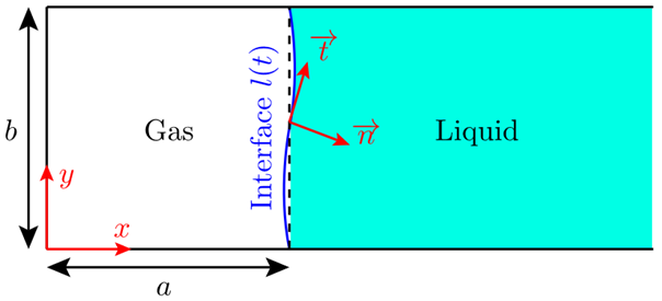
Figure 1: A schematic of the system under consideration. The base state and the deformed state of the interface are shown using dashed and curved line respectively.

In this work, our objective is to determine the resonant modes of a rectangular gas slug trapped at one end of a milli channel (Figure 1). We assume the gas liquid interface is flat and pinned at the base state. This can be achieved experimentally by having the milli-channel wall super hydrophilic where liquid is present and super hydrophobic where air is present. The surface can be maintained flat by controlling the gas pressure. The geometry considered mimics an acoustic micropump. The oscillations of the gas liquid interface which induces flow in the liquid are generated by ultrasound.

We restrict the analysis to two dimensions ($x$ and $y$) assuming the system extends to infinity in the z - direction. The deformation of the interface is explicitly specified as periodically oscillating function $l^{\star}(y^{\star},t^{\star})$. ($\star$ denotes that the variable has dimensions)

$$l^{\star}(y^{\star},t^{\star})=a(1-\varepsilon ih(y^{\star})e^{i\omega t^{\star}})$$ (1)

Here $a$ is the length of the undisturbed slug. $\varepsilon$ is the ratio of amplitude of oscillation to the base length of the slug. $h(y^{\star})$ is the yet to be determined deformation of the interface and $\omega$ denotes the angular frequency of oscillation of the bubble. We assume that the amplitude of deformation is much lower than the length of the slug ($\varepsilon<<1$). This enables us to analyse the system behavior using perturbation methods and matched asymptotics. We assume that the gas is inviscid, compressible and polytropic with $\Gamma$ as the polytropic coefficient. The liquid is assumed to be Newtonian and incompressible. The pinning of the interface implies $(h(0)=h(1)=0)$. These assumptions allow us to analyse the system in rectangular cartesian coordinates, while retaining the important physics.

II.1 Governing equation and characteristic scales

The dimensionless continuity Navier - Stokes equations are given as:

$$\frac{\partial u}{\partial t}+\varepsilon\mathbf{u}\cdot\nabla u=-\frac{\partial p}{\partial x}+\frac{1}{Re}\bigg{(}\frac{\partial^{2}}{\partial x^{2}}+k^{2}\frac{\partial^{2}}{\partial y^{2}}\bigg{)}u$$ (2)

$$\frac{\partial v}{\partial t}+\varepsilon\mathbf{u}\cdot\nabla v=-k^{2}\frac{\partial p}{\partial y}+\frac{1}{Re}\bigg{(}\frac{\partial^{2}}{\partial x^{2}}+k^{2}\frac{\partial^{2}}{\partial y^{2}}\bigg{)}v$$ (3)

Here $p,u,v$ are the dimensionless pressure, velocity components along $x$ and $y$ directions respectively in the liquid. All dimensionless variables are written without the $\star$ superscript. Also, $\mu$ and $\rho$ are the viscosity and density of the liquid respectively. The chosen characteristic length scales are, $x_{ch}=a$ and $y_{ch}=b$. We choose the time scale as $t_{ch}=1/\omega$ and the characteristic horizontal streaming velocity as $\varepsilon\omega a$. From continuity equation $(\nabla\cdot\mathbf{u}=0)$, we obtain the vertical characteristic velocity as, $v_{ch}=\varepsilon\omega b$.

Longuet Higgins [9] stated that cavitation microstreaming occurs at large Strouhal numbers $(Sl\simeq O(10^{2}))$. We define $\varepsilon=1/Sl=\frac{U_{ch}}{\omega a}$ as the smallness parameter, which will be used later for asymptotic analysis. $Re$ is the Reynolds number defined as $\frac{\omega a^{2}}{\nu}$. $p_{ch}=\varepsilon\rho\omega^{2}a^{2}$ is the characteristic pressure. $k$ is the aspect ratio of the rectangular bubble $(k=a/b)$. These equations are subject to the following dimensionless boundary conditions:

At walls:

$$\text{No slip and no penetration: }u=v=0\text{ at }y=0,1.$$ (4)

At liquid - gas interface:

$$\text{Zero tangential stress: }\mathbf{n}\cdot\mathbf{T}\cdot\mathbf{t}=0\text{ at }l(y,t)=1-\varepsilon ih(y)e^{i\omega t}.$$ (5)

$$\text{Kinematic condition: }\frac{\partial F}{\partial t}\frac{1}{|\nabla F|}\mathbf{u}\cdot\mathbf{n}=0\text{ at }x=l(y,t)$$ (6)

$$\text{Where, }F=x-l(y,t)\text{ represents the interface and }\mathbf{n}=\frac{\nabla F}{|\nabla F|}.$$

$$\text{Normal stress balance: }p_{i}-p+\frac{1}{Re}\tau_{xx}-\frac{1}{We}\kappa=0\text{ at }x=l(y,t).$$ (7)

Here $\mathbf{n}$ and $\mathbf{t}$ represent the normal and tangent vectors to the interface (Figure 1). $p_{i}$ and $p$ are the pressure in the gas phase and liquid phase respectively. $\tau_{xx}$ and $\kappa$ are the normal viscous stress and curvature of the interface. $\mathbf{T}$ represents the stress tensor at the interface. Also, $We$ is the Weber number, i.e., the ratio of inertial to surface tension forces $We=\frac{\rho\omega^{2}a^{2}}{\gamma/a}$.

III Method of solution

Our objective here is to obtain the resonant frequency of the system. Towards this, we solve the above system of dimensionless equations and obtain the surface modes on the interface. We seek solutions in the form of a perturbation series in $\varepsilon$ and use matched asymptotic expansions to account for boundary layer flow. We divide the domain into three regions: (i) an Inner region or Wall boundary layer and (ii) Outer region or Bulk and (iii) a Bubble boundary layer (near the gas liquid interface) as shown in Figure 2. The leading order velocity field is found separately in wall boundary layer and bulk region and matched to obtain a composite solution throughout the domain.

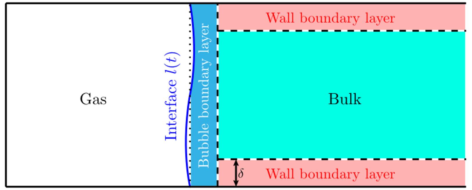
Figure 2: The bulk and wall boundary layer regions in the domain. The flow field is solved separately in these two regions and then matched to get the composite solution.

The solution to the governing system of equations is sought as a perturbation expansion in $\varepsilon$. Here velocity and pressure are expanded as a power series in $\varepsilon$ as:

$$u =u_{0}+\varepsilon u_{1}+O(\varepsilon^{2})$$

$$v =v_{0}+\varepsilon v_{1}+O(\varepsilon^{2})$$ (8)

$$p =p_{0}+\varepsilon p_{1}+O(\varepsilon^{2})$$

III.1 Zeroth order governing equations

Substituting the perturbation expansions (8) in the governing equations (2 and 3) and collecting the leading order terms yield:

$$\frac{\partial u_{0}}{\partial t} =-\frac{\partial p_{0}}{\partial x}+\frac{1}{Re}\bigg{(}\frac{\partial^{2}}{\partial x^{2}}+k^{2}\frac{\partial^{2}}{\partial y^{2}}\bigg{)}u_{0}$$

$$\frac{\partial v_{0}}{\partial t} =-k^{2}\frac{\partial p_{0}}{\partial y}+\frac{1}{Re}\bigg{(}\frac{\partial^{2}}{\partial x^{2}}+k^{2}\frac{\partial^{2}}{\partial y^{2}}\bigg{)}v_{0}$$ (9)

The subscript 0 in any variable throughout the paper denotes the zeroth/leading order solution. Exploiting the 2D nature of the flow field, we seek solutions to the above equations (9) using stream function formulation. The leading order velocity in terms of $\psi_{0}$ i.e., the leading order stream function is given by:

$$u_{0} =\frac{\partial\psi_{0}}{\partial y}$$

$$v_{0} =-\frac{\partial\psi_{0}}{\partial x}$$ (10)

After eliminating pressure, a modified biharmonic equation in $\psi_{0}$ is obtained:

$$\frac{\partial}{\partial t}\bigg{(}\frac{\partial^{2}}{\partial x^{2}}+k^{2}\frac{\partial^{2}}{\partial y^{2}}\bigg{)}\psi_{0}=\frac{1}{Re}\bigg{(}\frac{\partial^{2}}{\partial x^{2}}+k^{2}\frac{\partial^{2}}{\partial y^{2}}\bigg{)}^{2}\psi_{0}$$ (11)

The boundary conditions at the interface are defined for $x=l(y,t)$. We use domain perturbation around the steady flat interface to obtain the boundary conditions at $x=1$. This yields the dimensionless conditions:

$$\text{Kinematic boundary condition at the interface: }\frac{\partial\psi_{0}}{\partial y}\bigg{|}_{x=1}=h(y)e^{it}$$ (12)

$$\text{Tangential stress balance at interface: }\frac{\partial^{2}\psi_{0}}{\partial x^{2}}-k^{2}\frac{\partial^{2}\psi_{0}}{\partial y^{2}}\bigg{|}_{x=1}=0$$ (13)

$$\text{No slip and no penetration at the walls: }\frac{\partial\psi_{0}}{\partial y}=-\frac{\partial\psi_{0}}{\partial x}=0\text{ at }y=0,1.$$ (14)

$$\text{Normal stress balance at the interface: }p_{i}^{(0)}-p_{0}+\frac{1}{Re}\tau_{xx}^{(0)}-\frac{1}{\varepsilon We}\kappa\bigg{|}_{x=1}=0$$ (15)

We solve for the leading order problem using a semi–analytical approach. For this, we relax the no-slip condition at the walls and determine the horizontal slip velocity in the bulk region. This slip is matched with the horizontal velocity obtained by solving for the flow in the wall boundary layer.

III.1.1 Outer solution

The outer or bulk solution is valid in the region away from walls, where inertial effects are dominant. We seek solutions for the modified biharmonic equation, which are periodic in $y$ and $t$ as: $\psi_{0}=f(x)e^{i\lambda y}e^{it}$. The governing equation for $f$ is obtained by substituting this form of $\psi_{0}$ in the stream function equation (11)

$$f^{\prime\prime\prime\prime}(x)-(iRe+2k^{2}\lambda^{2})f^{\prime\prime}(x)+(k^{4}\lambda^{4}+iRek^{2}\lambda^{2})f(x)=0$$ (16)

$f^{\prime}(x)$ denotes first derivative of $f(x)$ w.r.t. x. The general solution to this equation (16) is :

$$f(x)=C_{1}e^{\xi x}+C_{2}e^{-\xi x}+C_{3}e^{-k\lambda x}+C_{4}e^{k\lambda x}$$ (17)

Here $\xi=\sqrt{iRe+k^{2}\lambda^{2}}$, which can also be written as $\xi=\sqrt{\alpha^{2}+k^{2}\lambda^{2}}$, where $\alpha=(1+i)/\delta$. The Reynolds number $Re$ is related to Stokes layer thickness $\delta$ as $Re=\frac{2}{\delta^{2}}$. The flow has to be bounded as $x\rightarrow\infty$. At high Reynolds numbers, $\frac{k^{2}\lambda^{2}}{Re}$ becomes a very small quantity. Hence the real part of $\xi$, $\Re(\xi)=\bigg{(}\frac{1}{4}+\frac{k^{4}\lambda^{4}}{4Re^{2}}\bigg{)}^{\frac{1}{4}}$ is a positive quantity. This implies the constants $C_{1}$ and $C_{4}$ must be zero so that $f(x)$ is bounded as $x\rightarrow\infty$. This implies:

$$f(x)=C_{2}e^{-\xi x}+C_{3}e^{-k\lambda x}$$ (18)

The no penetration boundary condition at the two walls yields $\lambda=n\pi$ for $n=0,1,2,3$. This gives us:

$$\psi_{0}=\sum_{n=0}^{\infty}(C_{2}e^{-\xi_{n}x}+C_{3}e^{-kn\pi x})\sin{n\pi y}\hskip 4.30554pte^{it}$$ (19)

The kinematic and tangential stress balance boundary condition (12, 13) gives the value of constants $C_{2}$ and $C_{3}$ as:

$$C_{2} =\sum_{n=0}^{\infty}A_{n}i\delta^{2}k^{2}n\pi e^{\xi_{n}}$$

$$C_{3} =\sum_{n=0}^{\infty}A_{n}\bigg{(}\frac{1}{n\pi}-i\delta^{2}k^{2}n\pi\bigg{)}e^{kn\pi}$$ (20)

Substituting these expressions in Equation 18, gives us:

$$\psi_{0}=\sum_{n=0}^{\infty}A_{n}\bigg{(}\frac{1}{n\pi}e^{-kn\pi s}+i\delta^{2}k^{2}n\pi(e^{-\xi_{n}s}-e^{-kn\pi s})\bigg{)}\sin{n\pi y}\hskip 4.30554pte^{it}$$ (21)

Here, $s=x-1$ and $A_{n}$ is the amplitude of the nth surface mode of the interface. The $O(\delta^{2})$ term in the expression represents the contribution from the bubble boundary layer as it decays much faster compared to the $O(1)$ term. We retain it in this formulation because it is multiplied by $k^{2}$.

While solving for this outer region, the no-slip boundary condition at the walls is not imposed. Instead, we obtain the horizontal slip velocity at $y=0,1$ from this bulk solution and match it with that obtained at the edge of the boundary layer to obtain the composite velocity field throughout the domain.

III.1.2 Inner solution close to the walls

To solve for the wall boundary layer, the $y$ variable is scaled as $\eta=y/\delta$ and $\eta=(1-y)/\delta$ near the bottom $(y=0)$ and top $(y=1)$ walls respectively. The stream function $\psi_{0}$ is also scaled as $\psi_{bl}=\frac{\psi_{0}}{\delta}$. This allows the flow in a small region close to the walls to be analyzed. This inner domain spans from $\eta=0$ at the walls to $\eta=\infty$ as $\delta<<1$. The rescaled stream function is governed by:

$$\frac{\partial}{\partial t}\bigg{(}\frac{\partial^{2}}{\partial x^{2}}+\frac{k^{2}}{\delta^{2}}\frac{\partial^{2}}{\partial\eta^{2}}\bigg{)}\psi_{bl}=\frac{1}{Re}\bigg{(}\frac{\partial^{2}}{\partial x^{2}}+\frac{k^{2}}{\delta^{2}}\frac{\partial^{2}}{\partial\eta^{2}}\bigg{)}^{2}\psi_{bl}$$ (22)

We seek $\psi_{bl}$ as $\psi_{bl}=g(x,\eta)e^{it}$ and impose the no slip and no penetration boundary conditions at the walls. As $\delta<<1$, the governing equation 22 reduces to:

$$\frac{2i}{k^{2}}\frac{\partial^{2}g}{\partial\eta^{2}}=\frac{\partial^{4}g}{\partial\eta^{4}}+O(\delta^{2})$$ (23)

Boundary conditions at the wall:

$$\text{No penetration: }\frac{\partial\psi_{bl}}{\partial x} =0\text{ at }\eta=0$$ (24)

$$\text{No slip: }\frac{\partial\psi_{bl}}{\partial\eta} =0\text{ at }\eta=0$$ .

We also consider that the horizontal velocity $(\partial\psi_{bl}/\partial\eta)$ is bounded as $\eta\rightarrow\infty$. Upon solving for $\psi_{bl}$, we get the expression:

$$\psi_{bl}=C(x)\bigg{(}\eta-\frac{1-i}{2}k\bigg{(}1-e^{-\frac{(1+i)\eta}{k}}\bigg{)}\bigg{)}e^{it}$$ (25)

Riley [2] analyzed the steady velocity induced close to a wall in the presence of a far-field oscillatory flow. Our solution matches with that of Riley when the aspect ratio, $k=1$. Our system that mimics a micro–pump can experimentally realize the boundary layer streaming described by Riley [2].

We match the dominant horizontal velocity at the edge of wall boundary layer with the bulk using Prandtl matching:

$$\frac{\partial\psi_{bl}}{\partial\eta}\bigg{|}_{\eta\rightarrow\infty}=\frac{\partial\psi_{0}}{\partial y}\bigg{|}_{y=0}\text{ for the lower and }\frac{\partial\psi_{bl}}{\partial\eta}\bigg{|}_{\eta\rightarrow\infty}=\frac{\partial\psi_{0}}{\partial y}\bigg{|}_{y=1}\text{ for the upper wall.}$$ (26)

This matching helps us determine $C(x)$. Using the value of $C(x)$ in Equation 25 gives the leading order stream function in the wall boundary layer:

$$\psi_{bl}=\sum_{n=0}^{\infty}A_{n}\big{(}e^{-kn\pi s}+i\delta^{2}k^{2}n^{2}\pi^{2}(e^{-\xi_{n}s}-e^{-kn\pi s})\big{)}\bigg{(}\eta-\frac{1-i}{2}k\bigg{(}1-e^{-\frac{(1+i)\eta}{k}}\bigg{)}\bigg{)}e^{it}$$ (27)

Here, $\eta=\frac{y}{\delta}$ for the bottom wall and $\eta=\frac{1-y}{\delta}$ for the top wall.

III.1.3 Composite leading order solution

We now determine the composite velocity field in the entire domain by combining the expression for flow in the bulk and boundary layer. For this, the ‘union’ of velocity field between bulk and boundary layers is determined. Since the velocity is continuous and purely horizontal at the edge of boundary layers, we add the bulk and boundary layer velocity fields and subtract the overlapping horizontal velocity magnitude to avoid double counting.

$$u_{comp} =u_{bulk}+u_{bl}-\big{(}u_{bulk}|_{y=0}+u_{bulk}|_{y=1}\big{)}$$

$$=\sum_{n=0}^{\infty}A_{n}\big{(}e^{-kn\pi s}+i\delta^{2}k^{2}n^{2}\pi^{2}(e^{-\xi_{n}s}-e^{-kn\pi s})\big{)}\big{(}\cos{n\pi y}-e^{\frac{-(1+i)y}{k\delta}}-e^{\frac{-(1+i)(1-y)}{k\delta}}\big{)}e^{it}$$ (28)

Note that here, the vertical velocity from the wall boundary layer $\big{(}\frac{\partial\psi_{bl}}{\partial x}\big{|}_{\eta\rightarrow\infty}\big{)}$ is neglected because it is of $O(\delta)$. It does not affect the composite solution as the vertical velocity that comes from the bulk at $y=0,1$ is also trivial. Substituting the horizontal composite velocity (28) in the leading order kinematic boundary condition (12) helps in determining the deformation $h(y)$ of the interface.

$$h(y)=\sum_{n=0}^{\infty}A_{n}\big{(}\cos{n\pi y}-e^{-\frac{(1+i)y}{k\delta}}-e^{-\frac{(1+i)(1-y)}{k\delta}}\big{)}e^{it}$$ (29)

The assumption of pinned interface implies, $h(y)$ must be zero at $y=0,1$. This implies $n$ must be even. We incorporate this by transforming $n\rightarrow 2n$. Hence, the velocity field and interface deformation is given as:

$$\mathbf{u_{0}}=\sum_{n=0}^{\infty}A_{n}\big{(}e^{-2kn\pi s}+4i\delta^{2}k^{2}n^{2}\pi^{2}(e^{-\xi_{n}s}-e^{-2kn\pi s})\big{)}\\ \bigg{(}\big{(}\cos{2n\pi y}-e^{\frac{-(1+i)y}{k\delta}}-e^{\frac{-(1+i)(1-y)}{k\delta}}\big{)}\mathbf{\hat{i}}+\sin{2n\pi y}\mathbf{\hat{j}}\bigg{)}e^{it}$$ (30)

$$h(y)=\sum_{n=0}^{\infty}A_{n}\big{(}\cos{2n\pi y}-e^{-\frac{(1+i)y}{k\delta}}-e^{-\frac{(1+i)(1-y)}{k\delta}}\big{)}e^{it}$$ (31)

Here $\xi_{n}=\sqrt{iRe+4k^{2}n^{2}\pi^{2}}$. The amplitudes of the overall deformation of the interface $A_{n}$s are determined using normal stress balance at the interface.

III.1.4 Finding the mode amplitudes of interface deformation

Our next objective is to find the amplitudes of each mode of interface oscillation ($A_{n}$). For this, we employ normal stress balance at the interface $x=l(t,y)$. Using domain perturbation in normal stress balance (15) results in:

$$p_{i}^{(0)}-p_{0}+\frac{1}{Re}\tau_{xx}^{(0)}-\frac{1}{\varepsilon We}\kappa\bigg{|}_{s=0}=0$$ (32)

This requires us to compute the dimensionless pressure inside ($p_{i}^{(0)}$) and outside ($p_{0}$) the bubble, curvature of interface ($\kappa$) and the dimensionless viscous stress ($\tau_{xx}^{(0)}$) at the interface. The liquid pressure just outside the interface ($p_{0}|_{s=0}$) is found by substituting the composite velocity field (30) into the leading order governing equation (11) and solving for pressure. This gives us the dimensionless pressure of the liquid just outside the interface to be:

$$p_{0}|_{s=0}=\bigg{(}\sum_{n=1}^{\infty}A_{n}i\bigg{(}\frac{4kn\pi}{\alpha^{2}}+\frac{1}{2kn\pi}\bigg{)}\cos{2n\pi y}+p_{0}^{\dagger}\bigg{)}e^{it}$$ (33)

Here $p_{0}^{\dagger}$ denotes the far-field non – dimensional oscillatory pressure amplitude observed as $s\rightarrow\infty$. We determine the dimensional pressure inside the gas bubble assuming that it undergoes polytropic expansion and contraction. We impose $PV_{initial}^{\Gamma}=PV_{final}^{\Gamma}$. Here $\Gamma$ is the polytropic coefficient. This gives us the pressure inside the bubble as:

$$p_{i}^{(0)}=p_{0}^{(i)}i\varepsilon\Gamma e^{it}\bigg{(}A_{0}+\sum_{n=1}^{\infty}\frac{2A_{n}k}{\alpha}\big{(}e^{\frac{-\alpha}{k}}-1\big{)}\bigg{)}$$ (34)

Here $p_{0}^{(i)}$ denotes the initial pressure inside the bubble. This is equal to the pressure close to the liquid at the base state. The dimensionless viscous stress tensor component ($\tau_{xx}$) is:

$$\tau_{xx}=\frac{\partial u_{comp}}{\partial x}=\sum_{n=0}^{\infty}A_{n}\big{(}-2kn\pi e^{-2kn\pi s}+4in^{2}\pi^{2}\delta^{2}k^{2}(-\xi_{n}e^{-\xi_{n}s}+2kn\pi e^{-2kn\pi s})\big{)}\\ \big{(}\cos{2n\pi y}-e^{-\frac{\alpha y}{k}}-e^{-\frac{\alpha(1-y)}{k}}\big{)}e^{it}$$ (35)

$$\tau_{xx}|_{s=0}=\sum_{n=0}^{\infty}A_{n}\big{(}-2kn\pi+4in^{2}\pi^{2}\delta^{2}k^{2}(-\xi_{n}+2kn\pi)\big{)}\bigg{(}\cos{2n\pi y}-e^{-\frac{\alpha y}{k}}-e^{-\frac{\alpha(1-y)}{k}}\bigg{)}e^{it}$$

The curvature $\kappa$ is found from the interface deformation $F=x-l(t,y)=0$ as:

$$\kappa=i\varepsilon e^{it}\sum_{n=0}^{\infty}A_{n}\bigg{(}-4n^{2}\pi^{2}\cos{2n\pi y}-\frac{\alpha^{2}}{k^{2}}\big{(}e^{-\frac{\alpha y}{k}}+e^{-\frac{\alpha(1-y)}{k}}\big{)}\bigg{)}$$ (36)

Substituting these expressions in (32) and collecting all the terms with $y$ dependency, we get a set of equations for $n=1$ to $\infty$ as:

$$\bigg{(}-\frac{\omega^{2}}{2n\pi k}\bigg{(}1+\frac{8k^{2}n^{2}\pi^{2}}{\alpha^{2}}\bigg{)}+\frac{2\mu i\omega kn\pi}{\rho a^{2}}+\frac{4n^{2}\pi^{2}\gamma k}{\rho a^{3}}\bigg{)}A_{n}\\ -\frac{2i\mu\omega}{\rho a^{2}}\bigg{(}\frac{4\alpha\big{(}1-e^{-\frac{\alpha}{k}}\big{)}}{4n^{2}\pi^{2}+\alpha^{2}}\bigg{)}\sum_{m=1}^{\infty}A_{m}m\pi\\ +\frac{\alpha^{2}\gamma}{\rho a^{3}k^{2}}\bigg{(}\frac{4\alpha\big{(}1-e^{-\frac{\alpha}{k}}\big{)}}{4n^{2}\pi^{2}+\alpha^{2}}\bigg{)}\sum_{m=0}^{\infty}A_{m}=0$$ (37)

We obtain another mathematical condition using the fact that the contact point must be stress-free for it to be pinned. This indicates that the stream function obtained from boundary layer ($\psi_{bl}$) must satisfy the tangential stress balance (13) at the surface. On simplifying, we obtain:

$$\sum_{n=0}^{\infty}A_{n}=O(\delta^{2})$$ (38)

$A_{n}$s are determined for a fixed set of $N+1$ modes. Here, $N$ stands for the maximum number of eigenmodes we use for computation. The value of $A_{n}$s decrease with increase in $n$ and so the higher modes have a lower contribution to the dynamics of the system. Equation (37) is divided by $\frac{\gamma k}{\rho a^{3}}$ to rewrite the normal stress balance in terms of dimensionless parameters.

$$\bigg{(}-\frac{\lambda^{2}}{2n\pi k^{2}}\bigg{(}1+\frac{8k^{2}n^{2}\pi^{2}}{\alpha^{2}}\bigg{)}+2ni\pi\lambda G+4n^{2}\pi^{2}\bigg{)}A_{n}\\ -\frac{i\lambda G}{k}\bigg{(}\frac{4\alpha\big{(}1-e^{-\frac{\alpha}{k}}\big{)}}{4n^{2}\pi^{2}+\alpha^{2}}\bigg{)}\sum_{m=1}^{N}A_{m}2m\pi\\ +\frac{\alpha^{2}}{k^{3}}\bigg{(}\frac{4\alpha\big{(}1-e^{-\frac{\alpha}{k}}\big{)}}{4n^{2}\pi^{2}+\alpha^{2}}\bigg{)}\sum_{m=0}^{N}A_{m}=0$$ (39)

$$\sum_{n=0}^{\infty}A_{n}=K\delta^{2}$$ (40)

Here, $\lambda=\frac{\omega}{\Omega}$ where $\Omega$ is a pre-factor used to non – dimensionalize angular frequency of surface mode oscillations. $G=\frac{\mu}{\sqrt{\rho a\gamma}}$ is the Ohnesorge number defined as the ratio of internal viscous dissipation to surface tension energy. $G$ determines the overall stability of bubble oscillation. Larger the $G$, lower will be the chances of bubble break off from the interface and lower will be the value of $A_{0}$ for a given frequency.

Equation 39 is a set of $N$ equations, such that $n$ goes from 1 to $N$. $A_{0}$ is obtained from equation 40 as $A_{0}=K\delta^{2}-\sum_{n=1}^{N}A_{n}$. $\delta$ is of the order of 0.1 for our system. $K$ is assumed to be a non – zero value $(K=0.1)$. It is seen in our calculations that changing the value of $K$ does not change the results obtained.

We express the interface deformation (31) in terms of a Fourier cosine series for determining the resonant frequency of various modes. This further facilitates comparison with experiments. For this, the interface deformation is rewritten as $\sum_{n=0}^{M}a_{n}e^{i\phi_{n}}\cos{2n\pi y}$. These $a_{n}$s indicate the amplitude of each surface mode. We determine the interface deformation for a range of driving frequencies ($\omega$) and obtain the corresponding $a_{n}$ values. The maxima of $a_{n}$ for each mode corresponds to the resonance frequency of that mode.

The zeroth order flow field obtained is purely oscillatory. In order to obtain the observable streaming in the system, we seek solutions to the first-order system.

III.2 First order analysis

The equation governing the flow field at the first order in $\varepsilon$ is similar to unsteady Stokes equation with a source term given by the Reynolds stress evaluated using zeroth order flow field.

$$\frac{\partial(E^{2}\psi_{1})}{\partial t}-\frac{\partial(\psi_{0},E^{2}\psi_{0})}{\partial(x,y)}=\frac{1}{Re}E^{4}\psi_{1}$$ (41)

$E^{2}$ is a modified Laplacian operator in the system given by $E^{2}=\frac{\partial^{2}}{\partial x^{2}}+k^{2}\frac{\partial^{2}}{\partial y^{2}}$. $\psi_{1}$ denotes the stream function describing the first order flow field. The Jacobian term in the equation denotes the Reynolds stress. This non – homogeneity in the system is of $O(\delta^{2})$ and is significant only very close to the interface.

$$\frac{\partial(\psi_{0},E^{2}\psi_{0})}{\partial(x,y)}=\frac{\partial\psi_{0}}{\partial x}\frac{\partial(E^{2}\psi_{0})}{\partial y}-\frac{\partial\psi_{0}}{\partial y}\frac{\partial(E^{2}\psi_{0})}{\partial x}$$ (42)

The solution ($\psi_{1}$) has a time periodic and a steady part. We seek the latter which contributes to the observable streaming in the system. Towards this, we time average Equation 41 over one cycle. Denoting the time average by $<>$, we obtain,

$$\bigg{<}\frac{\partial^{4}\psi_{1}}{\partial x^{4}}+2k^{2}\frac{\partial^{4}\psi_{1}}{\partial x^{2}\partial y^{2}}+k^{4}\frac{\partial^{4}\psi_{1}}{\partial y^{4}}\bigg{>}=-Re\bigg{<}\frac{\partial(\psi_{0},E^{2}\psi_{0})}{\partial(x,y)}\bigg{>}$$ (43)

These are subject to:

$$\text{Kinematic boundary condition at the interface: }\bigg{<}\frac{\partial\psi_{1}}{\partial y}\bigg{>}\bigg{|}_{s=0}=-\bigg{<}\frac{\partial\psi_{sd}}{\partial y}\bigg{>}$$

$$\text{Tangential stress balance at interface: }\bigg{<}\frac{\partial^{2}\psi_{1}}{\partial x^{2}}-k^{2}\frac{\partial^{2}\psi_{1}}{\partial y^{2}}\bigg{>}\bigg{|}_{s=0}=-\bigg{<}\frac{\partial^{2}\psi_{sd}}{\partial x^{2}}-k^{2}\frac{\partial^{2}\psi_{sd}}{\partial y^{2}}\bigg{>}$$ (44)

$$\text{No slip and no penetration at the walls: }\bigg{<}\frac{\partial\psi_{0}}{\partial y}\bigg{>}=-\bigg{<}\frac{\partial\psi_{0}}{\partial x}\bigg{>}=0\text{ at }y=0,1.$$

Stokes in 1847 [17] established that the time averaged Lagrangian and Eulerian velocities differ by a velocity magnitude called Stokes Drift. Here $\psi_{sd}$ denotes the stream function that corresponds to Stokes drift in the system. Lagrangian stream function quantifies the fluid particle velocity also known as the observable streaming velocity in the system. The Stokes drift is a correction to the Eulerian velocity for calculating this observable flow field $(\psi_{Lagrangian}=\psi_{Eulerian}+\psi_{Stokes\hskip 1.50694ptDrift})$. Here $\psi_{1}$ is the Eulerian stream function. Following Longuet Higgins [9], Stokes drift is given as:

$$\psi_{Stokes\hskip 3.01389ptDrift}=\bigg{<}\frac{\partial\psi_{0}}{\partial y}\int\frac{\partial\psi_{0}}{\partial x}dt\bigg{>}$$ (45)

According to Bruus et al. [18], the flow in the bulk is driven by two contributions. These are the Reynolds Stress appearing in the governing equation and the slip generated by the wall boundary layer. Our interest is in the flow field generated far away from the bubble. So, we neglect the contribution from the interface (Reynolds stress) and focus on finding the velocity field by assuming that the only contribution to the flow is from the wall boundary layer slip.

The time–averaged system is governed by Stokes flow with a slip at each of the walls. As a first step, we find the first order slip generated at the edge of the wall boundary layer.

III.2.1 Inner region close to the wall

The first order flow in the wall boundary layer is solved by rescaling the $y$ coordinate as $\eta=y/\delta$ at the bottom wall and $\eta=(1-y)/\delta$ at the top wall. The dependent variable is also rescaled as $\psi_{1,bl}=\psi_{1}/\delta$. Then the time-averaged first order governing equation simplifies to:

$$k^{2}\frac{\partial^{4}\big{<}\psi_{1,bl}\big{>}}{\partial\eta^{4}}=-2\bigg{(}\bigg{<}\frac{\partial\psi_{0,bl}}{\partial x}\frac{\partial\big{(}\frac{\partial^{2}\psi_{0,bl}}{\partial\eta^{2}}\big{)}}{\partial\eta}\bigg{>}-\bigg{<}\frac{\partial\psi_{0,bl}}{\partial\eta}\frac{\partial\big{(}\frac{\partial^{2}\psi_{0,bl}}{\partial\eta^{2}}\big{)}}{\partial x}\bigg{>}\bigg{)}$$ (46)

This is subject to :

$$\text{No slip and no penetration at the walls: }\bigg{<}\frac{\partial\psi_{1,bl}}{\partial\eta}\bigg{>}=0\text{ at }\eta=0.$$

$$\text{Flow being bounded far away from the wall: }\bigg{<}\frac{\partial\psi_{1,bl}}{\partial\eta}\bigg{>}\bigg{|}_{\eta\rightarrow\infty}=0.$$

For the time averaging of the Jacobian, we use the identity, $Ae^{it}Be^{it}=\frac{1}{2}A\overline{B}=\frac{1}{2}\overline{A}B$. Here $\overline{B}$ corresponds to the conjugate of $B$. We find the slip at the edge of the wall boundary layer as:

$$\frac{\partial\psi_{1,bl}}{\partial\eta}\bigg{|}_{\eta\rightarrow\infty}=\bigg{(}-\frac{5}{8}+\frac{11i}{8}\bigg{)}\overline{U}\frac{dU}{dx}+\bigg{(}-\frac{1}{8}+\frac{5i}{8}\bigg{)}\frac{d\overline{U}}{dx}U$$ (47)

Here $U(x)$ is obtained from $\psi_{0,bl}=U(x)(\eta-(1-i)/2k(1-e^{-(1+i)\eta/k}))e^{it}$. The real part of this expression simplifies to $-\frac{3}{8}\big{(}(1+i)U\frac{d\overline{U}}{dx}+(1-i)\overline{U}\frac{dU}{dx}\big{)}$, which is identical to the steady slip velocity found by Riley [2]. Riley found that the observable slip generated by the wall boundary layer when a far–field oscillatory flow given by $u(x)e^{it}$ acts on the bulk region is given by $-\frac{3}{8}\big{(}(1+i)u\frac{d\overline{u}}{dx}+(1-i)\overline{u}\frac{du}{dx}\big{)}$. In our system, $U(x)$ is the leading order horizontal velocity in bulk region at $y=0,1$. We neglect the $O(\delta^{2})$ term in $U(x)$ and this gives:

$$U(x)=\sum_{n=0}^{\infty}A_{n}e^{2kn\pi s}$$ (48)

Thus, the real part of slip at the edge of boundary layer (47) is given by:

$$\frac{\partial\psi_{1,bl}}{\partial\eta}\bigg{|}_{\eta\rightarrow\infty}=\sum_{n=0}^{\infty}\sum_{m\geq n}^{\infty}\frac{3}{2(1+\delta_{mn})}a_{m}a_{n}e^{-2k(m+n)\pi s}k\pi\big{(}(m+n)\cos{\psi_{m,n}}\\ +(m-n)\sin{\phi_{m,n}}\big{)}$$ (49)

Here $\delta_{mn}$ is the Kronecker delta function. Each mode amplitudes $A_{n}$ is rewritten in terms of the Fourier amplitudes ($a_{m}$) and phase angles $(\phi_{m})$ from the corresponding interface deformation $h(y)$. $\phi_{m,n}$ indicates the phase difference $\phi_{m}-\phi_{n}$. This slip (Equation 49) is the maximum observable Eulerian velocity attained in the bulk, far away from the bubble, and it drives the entire bulk flow.

III.2.2 Bulk lagrangian flow

Figure 3: The modified first-order system that we solve for in the bulk.

The governing equation for bulk flow are:

$$\bigg{<}\frac{\partial^{4}\psi_{1,e}}{\partial x^{4}}+2k^{2}\frac{\partial^{4}\psi_{1,e}}{\partial x^{2}\partial y^{2}}+k^{4}\frac{\partial^{4}\psi_{1,e}}{\partial y^{4}}\bigg{>}=0$$ (50)

This governing equation is subject to the slip given by equation 49 at $y=0,1$. To evaluate this, we first integrate the slip at the walls and obtain the stream function at $y=0,1$. We get:

$$\psi_{1,e}|_{y=0,1}=\sum_{n=0}^{\infty}\sum_{m\geq n}^{\infty}\frac{3}{4(1+\delta_{mn})}a_{m}a_{n}e^{-2k(m+n)\pi s}k\bigg{(}\cos{\phi_{m,n}}+\frac{m-n}{m+n}\sin{\phi_{m,n}}\bigg{)}$$ (51)

The slip is already in the form of an eigenfunction in $x$ direction for the governing equation 50. We can obtain a valid solution to the flow field by simply multiplying $\sin{2(m+n)\pi y}$. Thus, the stream function in the bulk is given by:

$$\psi_{1,e}|_{y=0,1}=\sum_{n=0}^{\infty}\sum_{m\geq n}^{\infty}\frac{3}{4(1+\delta_{mn})}a_{m}a_{n}e^{-2k(m+n)\pi s}k\\ \bigg{(}\cos{\phi_{m,n}}+\frac{m-n}{m+n}\sin{\phi_{m,n}}\bigg{)}\sin{2(m+n)\pi y}$$ (52)

The Stokes drift correction factor must be added to obtain the Lagrangian velocity in the bulk. The real part of Stokes drift can be calculated from Equation 45 as:

$$\psi_{sd}=\sum_{n=0}^{\infty}\sum_{m\geq n}^{\infty}-\frac{1}{4(1+\delta_{mn})}a_{m}a_{n}\big{(}\sin{\phi_{m,n}}k\delta\\ -2n\pi(\cos{\phi_{m,n}}-\sin{\phi_{m,n}})k^{2}\delta^{2}+O(\delta^{3})\big{)}\sin{2(m+n)\pi y}$$ (53)

Neglecting higher order terms, the Lagrangian stream function $(\psi_{L})$ is obtained by adding $\psi_{sd}$ and $\psi_{1,e}$:

$$\psi_{L}=\psi_{1,e}+\psi_{sd}=\\ \sum_{n=0}^{\infty}\sum_{m\geq n}^{\infty}\frac{k}{4(1+\delta_{mn})}a_{m}a_{n}\bigg{(}\bigg{(}-\delta+\frac{m-n}{m+n}e^{-2k(m+n)\pi s}\bigg{)}\sin{\phi_{m,n}}\bigg{)}\\ +e^{-2k(m+n)\pi s}\cos{\phi_{m,n}}\bigg{)}\sin{2(m+n)\pi y}$$ (54)

Notice that here, as $s\rightarrow\infty$ the slip generated by this flow is linear in $k$.

$$\frac{\partial\psi_{L}}{\partial y}\bigg{|}_{s\rightarrow\infty}=\sum_{n=0}^{\infty}\sum_{m\geq n}^{\infty}a_{m}a_{n}\sin{\phi_{m,n}}\frac{-k\delta(m+n)\pi}{2(1+\delta_{mn})}$$ (55)

This implies that the magnitude of observable slip generated linearly increases with increase in aspect ratio of bubble at large distances from the interface. This can be used by future experimentalists to fabricate their systems for a required flow rate by simply manipulating the size of the bubble. We see that the slip at the walls is negative, indicating a pulling effect near the walls. The pulling effect at the walls tends to push the bulk fluid away from the bubble, thereby creating a pumping effect. We next use numerical simulations to validate our findings from the analytical approach.

IV Numerical Analysis

The analytical approach helps determine the resonant frequency for each surface mode. We numerically simulate the system at these frequencies to obtain the observable flow field. We compare the numerically obtained observable slip at the walls with the result obtained theoretically. This helps us obtain an independent verification of the semi analytical results. To have an unbiased comparison, we use the far field pressure found analytically for the numerical simulations.

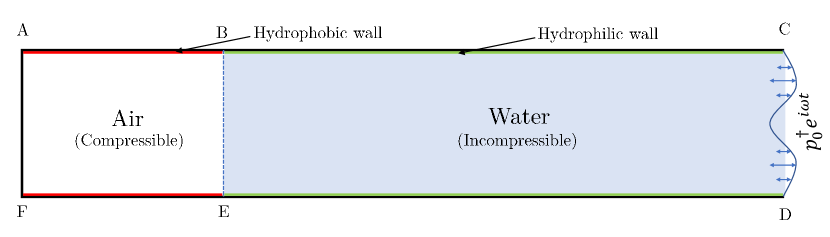
Figure 4: Two-dimensional ANSYS model used to simulate the oscillations of a pinned gas slug.

We model the system shown in Figure 4 using Volume of Fluid approach in ANSYS. The length of liquid in the channel (10 mm) is chosen much larger than the length of the gas slug to mimic its extending to infinity. We assign the pressure that was found theoretically from semi-analytical investigation, i.e., $p_{0}^{\dagger}e^{i\omega t}$ (Equation 32) at the right boundary of the domain as a pressure – inlet. Note that here, the magnitude of $p_{0}^{\dagger}$ is approximately 20 kPa with negligible change across different $k$ values. Air is assumed to be compressible and follows polytropic expansions and contractions. Water is assumed incompressible. Surface tension between the fluids is taken as 0.0725 N/m. The part of the wall exposed to air is assumed to be super hydrophobic, while the wall region wetted by the liquid is assigned as super hydrophilic. This is done to prevent horizontal movement of the contact line and hence ‘pin’ the interface to the wall.

Table 1: Settings used in Ansys Fluent

Description	Setting
Coordinates and Solver type	2D (Transient)
Model properties for air (Compressible)
Specific heat	1006.43 J/(kg K) (default)
Thermal conductivity	0.0242 W/(m K) (default)
Viscosity	1.7894 $\times$ $10^{-5}$ kg/(m s) (default)
Molecular weight	28.966 kg/mol (default)
Standard state enthalpy	0 J/kg mol (default)
Reference temperature	298.15 K (default)
Density	ideal – gas model
Model properties for water (Incompressible)
Specific heat	4182 J/(kg K) (default)
Thermal conductivity	0.6 W/(m K) (default)
Viscosity	0.001003 kg/(m s) (default)
Molecular weight	18.0152 kg/mol (default)
Standard state enthalpy	$-2.858\times 10^{8}$ J/kgmol (default)
Reference temperature	298 K(default)
Density	998.2 kg/$m^{3}$(default)
Mesh size, time step, and run initialization
Mesh resolution	3130 $\times$ 100 grids
Convergence criteria	$10^{-3}$
Maximum iterations	5000
Time step	$10^{-6}$ s
Model and boundary conditions
Models used	Multiphase (Volume of Fluid), Viscous (Transition SST)
Phase interaction	Constant surface tension = 0.0725 N/m. Continuum surface force modelling with wall adhesion.
Boundary conditions	Pressure inlet at side CD is given by Eq. 32 Walls AB, FE are hydrophobic with (Air – water contact angle $0^{0}$) Walls BC, ED are hydrophilic with (Air – water contact angle $180^{0}$) All walls also follow no slip and no penetration boundary condition except the pressure inlet CD.
Solution methods and discretization schemes
Pressure – velocity coupling scheme	PISO
Gradient	Green – Gauss Node Based
Pressure	PRESTO!
Density, Momentum, Turbulent Kinetic Energy, Specific Dissipation Rate, Intermittency, Momentum Thickness Re, Energy	Second Order Upwind
Volume Fraction	Geo Reconstruct
Particle injection data
Type of particle	Inert, Anthracite
Injection type	Along surface of the entire domain
Diameter of particles	2 $\mu m$ (uniform)
Start and stop time of injection	1 ms to 1.5 ms
DPM Model: Number of steps	20000
DPM Model: Type	Unsteady particle tracking

We run the simulation at the resonant frequencies obtained for different mode amplitudes. We also insert inert ‘anthracite’ particles of 2 $\mu m$ diameter into the stream using discrete particle model in Ansys FLUENT. This helps us to find the observable fluid velocity in the system. This enables us to compare the theoretically obtained Lagrangian slip with particle velocity obtained close to the wall.

V Results and discussions

V.1 Mode amplitudes as a function of driving frequency

The Fourier amplitude of mode $n$ ($a_{n}$) is plotted against the driving frequency to obtain the resonant frequency for each mode. For all computations, the total number of amplitude modes considered is $N$. $M$ is the maximum number of Fourier modes used to describe the interface deformation. In all simulations, we consider $N=20$ and $M=50$. The results are insensitive to the values of $N$, $M$ if they are above 5. Higher number of modes give better accuracy. In the supplementary material (Section 2), the results for different $N$ values are compared.

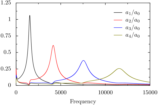
Figure 5: The amplitude modes for a slug of 1.6 mm length and 0.374 mm width with water as surrounding fluid, mimicking the experiments performed by Ryu et.al. [1] Maxima for each amplitude mode occur at 1.533 kHz, 4.161 kHz, 7.547 kHz, and 11.545 kHz respectively.

Figure 5 shows the different normalized mode amplitudes plotted against the driving frequency for a slug of 1.6 mm length and 0.374 mm width surrounded by water. These parameters are chosen to mimic the experiments of Ryu et al. [1] by using the height of interface from the left wall as $a$ and tube diameter as $b$. We see that the maximum amplitude of each succeeding mode is lower than the previous one. With an increase in frequency, the different surface modes of oscillation become more prominent. This is observed experimentally in both spherical [11] as well as semi – cylindrical [12] bubbles. The predicted resonance frequency of the second mode, 4.161 kHz, is comparable to that obtained experimentally by Ryu et al [1]. The experimental images of their work suggest oscillations corresponding to the second mode at approximately 4 kHz. Consequently, the resonant peak of the second mode obtained in our study coincides with the experimental resonance frequency observed in their study.

V.1.1 Leading order interface deformation

We now discuss the shape of the deformed interface for the first mode for illustration. At this mode, we expect the total number of maxima and minima of the interface to be 3. The peripheral maxima are a result of the exponential part of the interfacial deformation expression that causes pinning of the interface. The $A_{n}$ values are substituted in Equation 31 to determine the gas–liquid interface deformation at a frequency of 1.333 kHz.

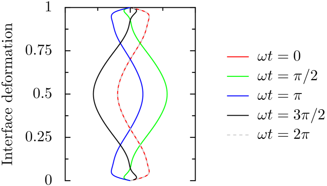
Figure 6: Purely oscillatory interface deformation calculated for a bubble of 1.6 mm length and 0.374 mm width, surrounded by water at $25^{0}$C and driven at 1.3 kHz.

Figure 6 shows snapshots at different time instants of the interface. This confirms the periodic nature of interface deformation for the second mode. The leading order interface oscillations are periodic with a time period of $2\pi/\omega$ which is explicitly specified in the model. The amplitude of interface deformation shown is scaled with $\varepsilon a$. The magnified version depicted in Figure 6 shows that the interface displacement is zero at the walls, thereby satisfying the pinning condition.

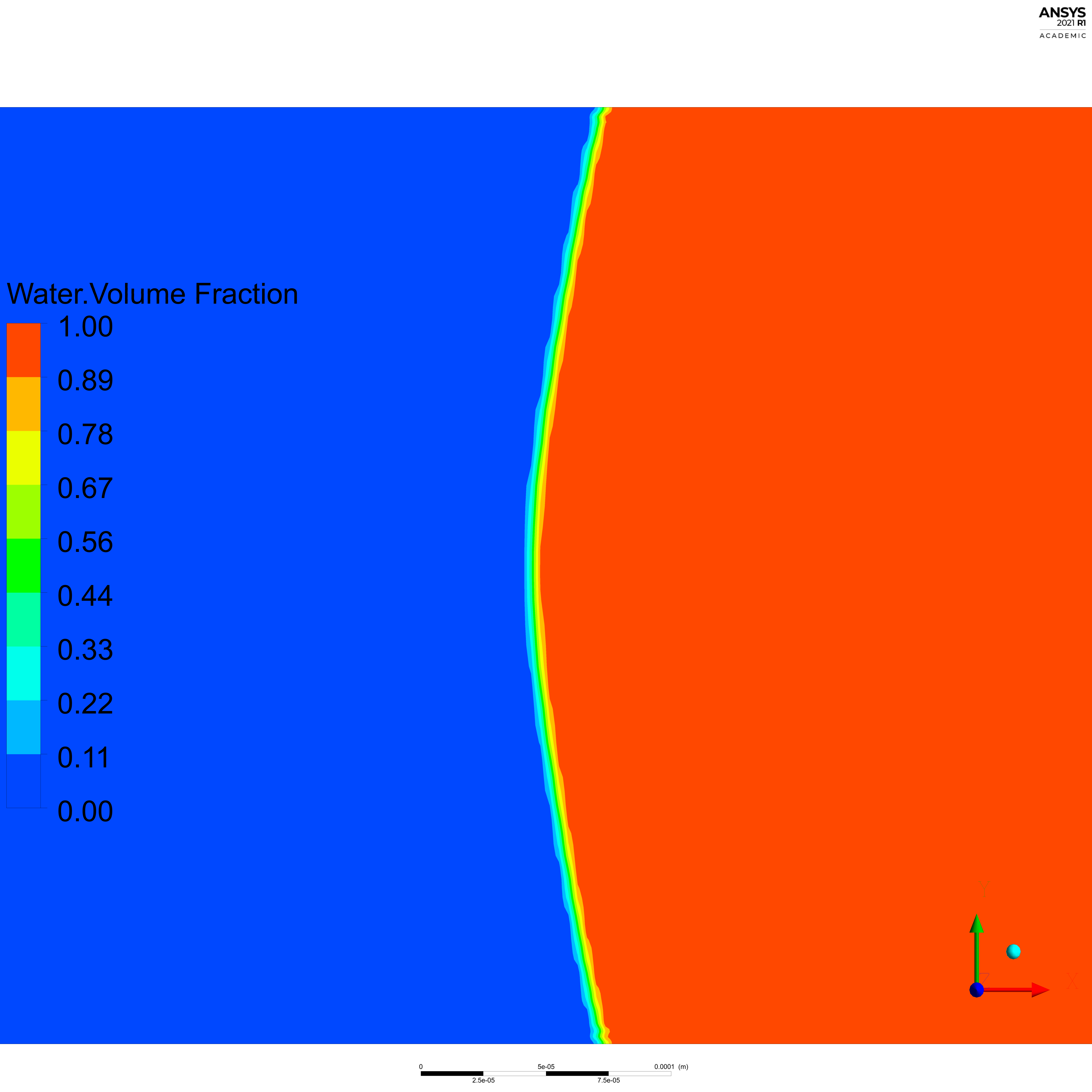
(a)

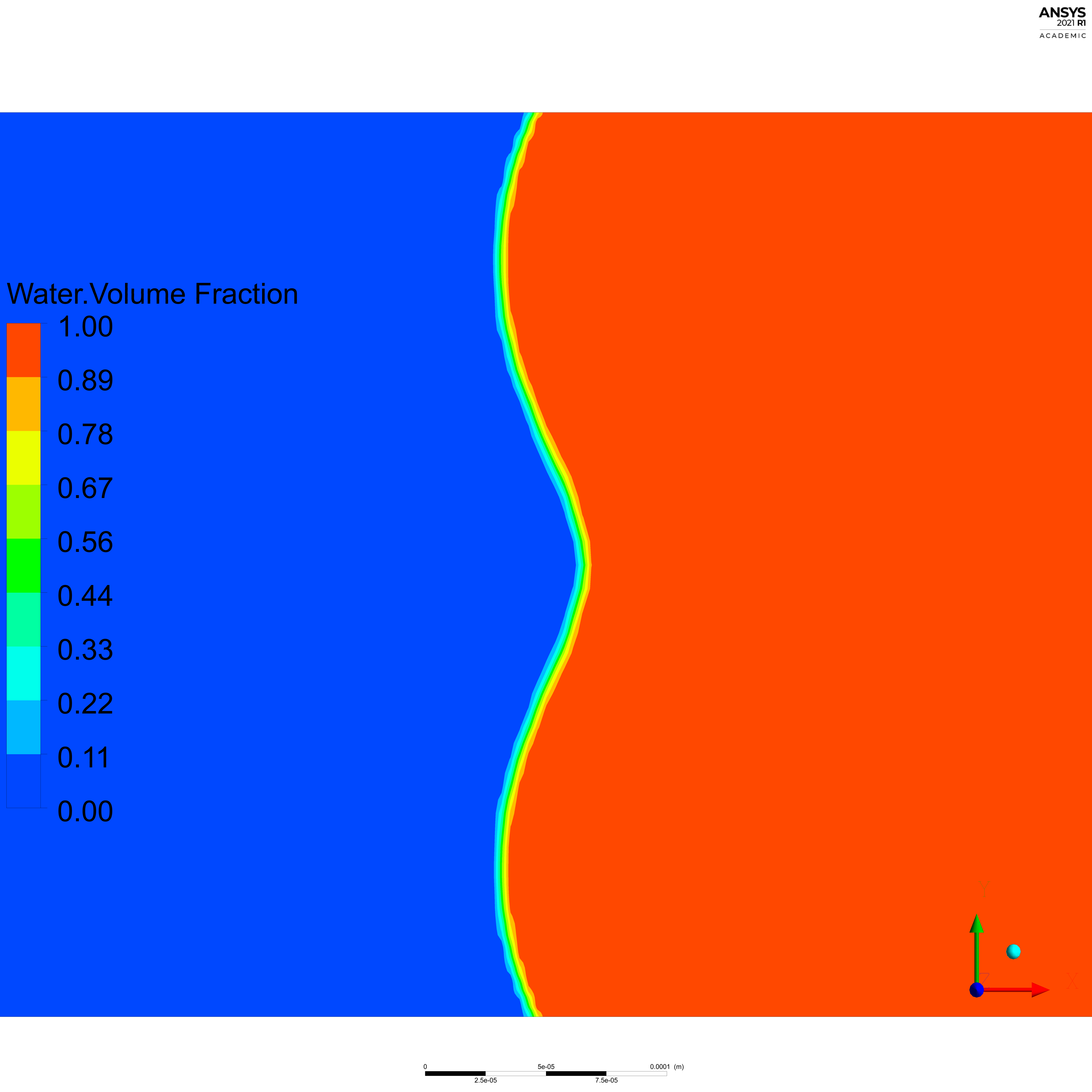
(b)

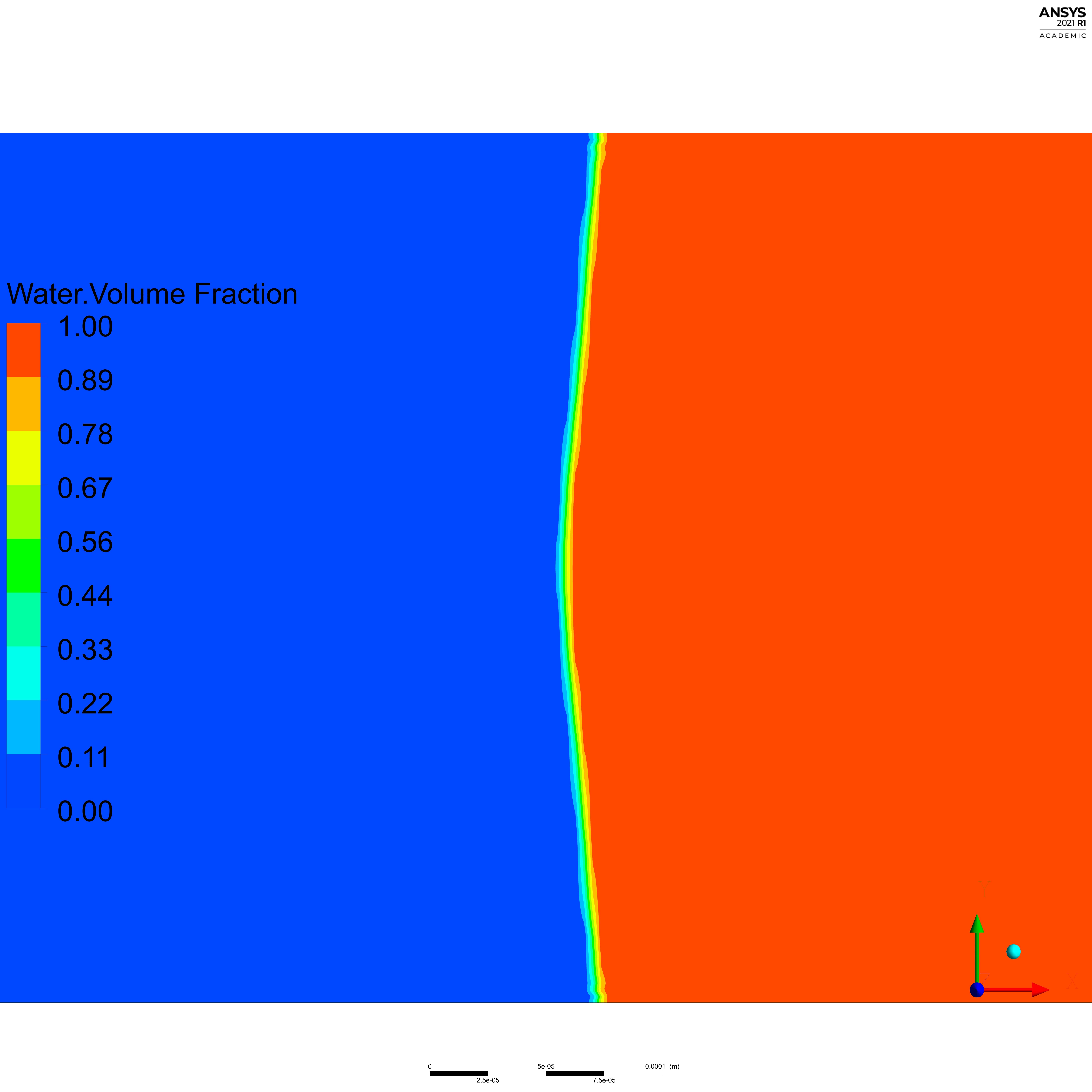
(c)

Figure 7: The three modes observed in numerical simulations, pertaining to (a) First mode: 1.333 kHz (b) Second mode: 4.161 kHz and (c) Third mode: 7.547 kHz respectively. The length of the bubble is 0.8 mm, and the width of the channel is 0.374 mm. All the other parameters are given in Table LABEL:ansystable

We depict the numerically obtained interface deformation from simulations in ANSYS in Figure 7. We see that there is good qualitative agreement at the resonant frequencies for the first and second modes. At the resonant frequency for the third mode, the gas slug exhibits volumetric expansion first. Three modes develop on the surface of the expanded gas slug. This can be seen in the video in supplementary (See section 3 in supplementary material). The numerical simulations confirm the occurrence of different modes at varying frequencies i.e., as the frequency is increased a higher number of modes is observed.

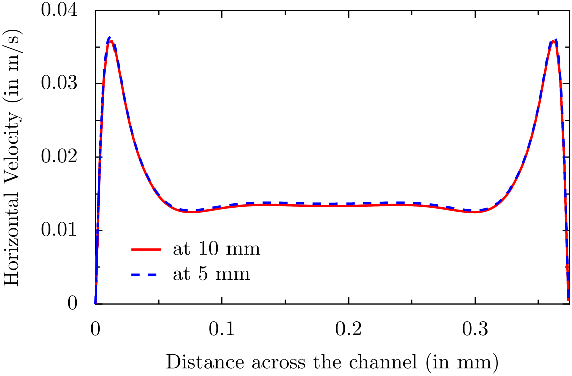
Figure 8: The horizontal Eulerian velocity across the width of the channel measured using ANSYS Fluent at distances 5 mm and 10 mm from the plane AF of the channel (See Figure 4). The pressure is oscillated at 7.547 kHz. (Peak corresponding to the third mode). The other parameters are mentioned in Table LABEL:ansystable.

In Figure 8, we depict the variation of the horizontal velocity across the width of the channel at two different axial locations. The peaking of velocity shows that there exists an Eulerian slip at the wall boundary layer which is persistent even at long distances from the slug. This is consistent with our finding that there exists an Eulerian slip at the wall boundary layer, which is persistent even at long distances from the slug. This is consistent with our finding that there is a zeroth order slip arising from the wall boundary layer. The distance of the peaks from the wall do not vary much with axial position. This indicates that the wall boundary layer thickness varies negligibly with distance from the interface.

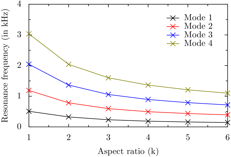
(a)

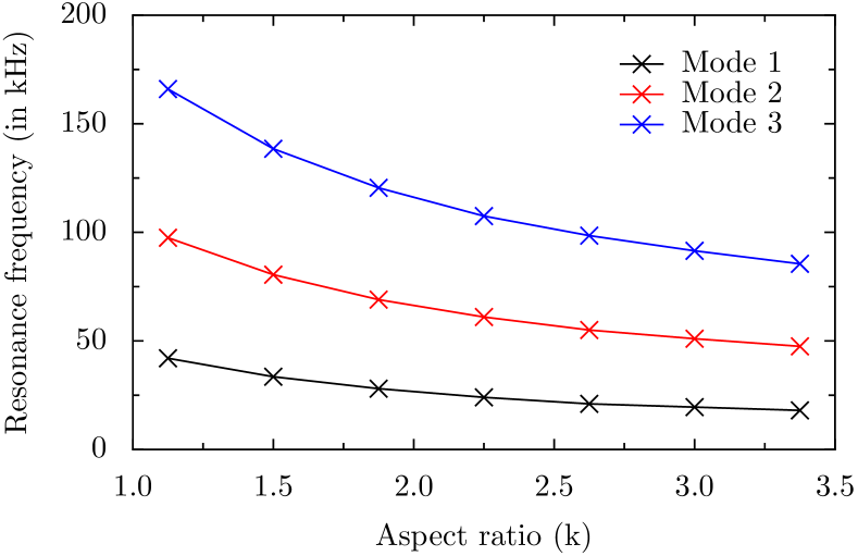
(b)

Figure 9: Resonance frequency variation with increase in aspect ratio for milli (a) and micro (b) channels. Fluid properties correspond to water at room temperature. The width of the channel ‘$b$’ values are (a) 1.6 mm and (b) 80 $\mu$m.

A control parameter that can be used to control the system behavior is the slug size. For milli and micro bubbles, the dependence of resonance frequency on the aspect ratio of the bubble was investigated analytically (See Figure 9). We see a decrease in resonance frequency with increase in aspect ratio of the bubble. This is similar to the trend for Minnaert frequency which decreases with increase in size of the bubble.

Figure 10: Comparison of theoretically obtained horizontal Lagrangian slip velocity at the walls (orange line) to the numerically obtained horizontal particle velocity close to the walls (blue line) for different aspect ratio of bubble.

In Figure 10, we compare the Lagrangian slip velocity at the edge of wall boundary layer obtained analytically (Equation 55) with the particle velocity obtained from ANSYS Fluent very close to the walls. Increasing the slug length for a fixed driving frequency increases the magnitude of observable streaming velocity generated in the fluid. This linear dependence arises mainly from the Stokes drift in the system. The magnitude of the velocity estimated analytically is of the same order of magnitude as that obtained numerically. The non – monotonic variation of the velocity with aspect ratio arises from the phase difference between the different modes. It must be borne in mind that we have neglected all direct contribution from the interface to the observable streaming in our analytical approach.

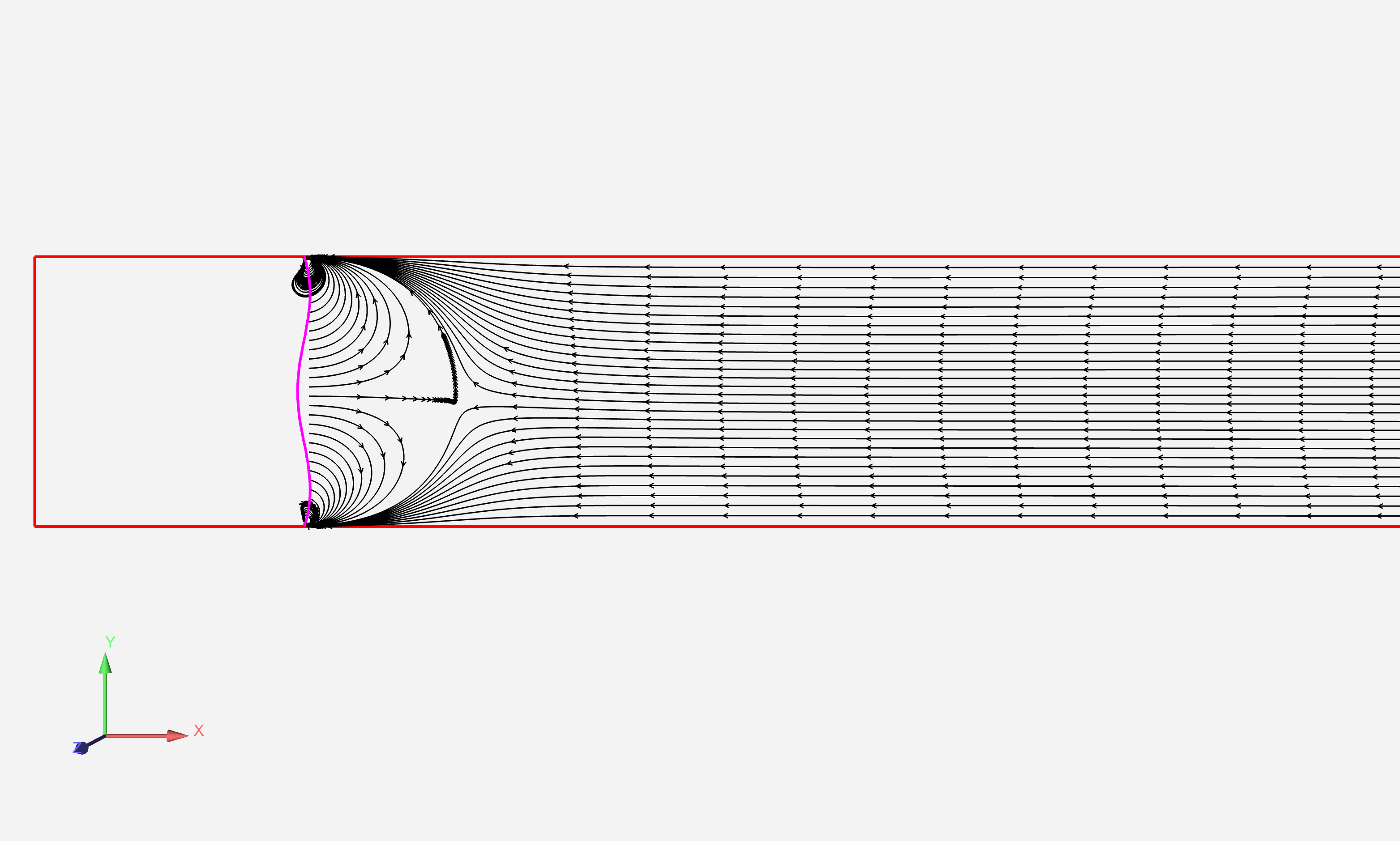
(a)

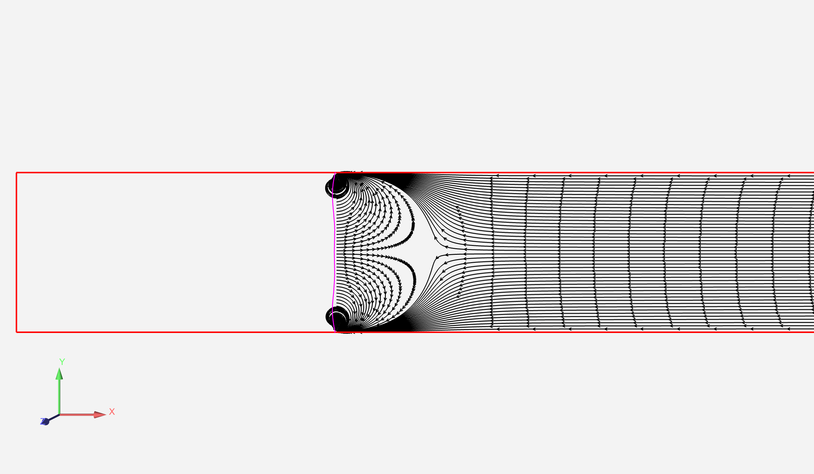
(b)

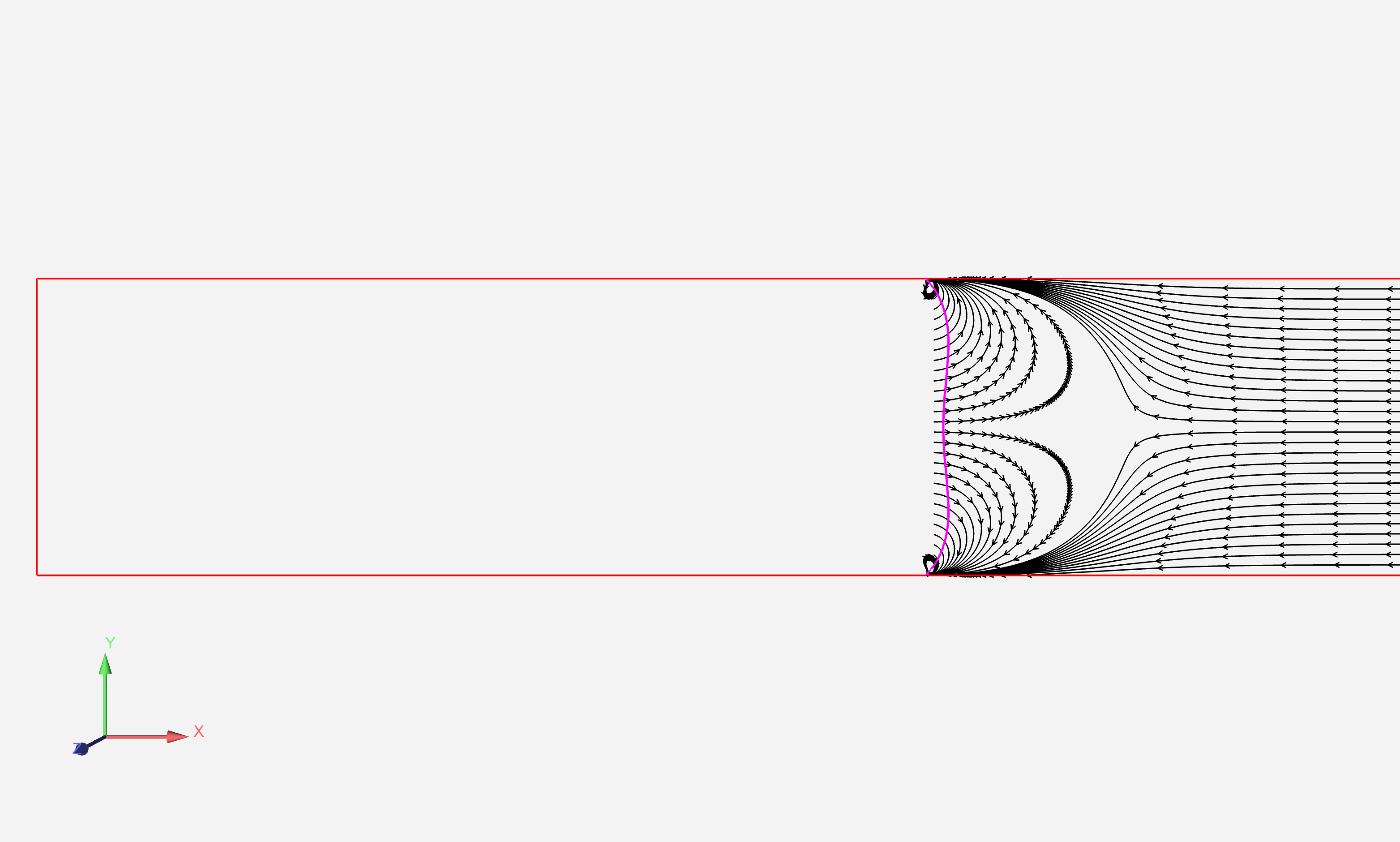
(c)

Figure 11: The trajectories of inert particles towards the interface when released at a distance of 5 mm from the left most wall AF in Figure 4. The width of the channel is 0.374 mm. Physical properties are mentioned in Table LABEL:ansystable. Aspect ratio ($k$) values are (a) 1 (b) 2 and (c) 3.

In Figure 11, we see that the particles get trapped in closed vortices very close to the interface. The size of the vortex in which these particles get trapped keeps reducing with increase in aspect ratio of channel. The presence of these vortices is also observed in experiments and has been exploited by researchers in particle segregation, and concentration. As predicted by theory, the particles move towards the interface closer to the stationary walls.

VI Conclusions

This work focusses on developing a theoretical framework to predict the resonance frequency of a trapped bubble in a milli channel. This system helps understand the behavior of an acoustic micropump/micromixer using mostly a leading order analysis. We show that a cartesian system is enough to predict the resonant frequency of a trapped gas slug system operating at high Strouhal numbers. By introducing different scaling along $x$ and $y$ coordinates, we have shown the effect of length of slug used for trapping the oscillating bubble in experiments. The effect of this length has been ignored in almost all analytical studies because of the predominant applications for sessile semi - cylindrical or spherical bubbles. However, our study shows that resonance frequency decreases with increase in slug length. The resonance frequency calculated from leading order analysis is in good agreement with that found in the experiments done by Ryu et.al. [1]

We use numerical simulations with ANSYS Fluent to confirm that the resonant frequencies obtained theoretically match with the numerical results by qualitatively comparing various interfacial modes that are observed on the bubble. It was also found that there exists a region close to the wall, where horizontal flow is maximum and that the thickness of this wall boundary layer does not change with distance from the interface. The steady streaming velocity obtained theoretically was found to match reasonably well with that obtained numerically. The dependency of the streaming velocity on the aspect ratio predicted by both analytical and numerical approaches is similar.

References

- Ryu et al. [2010] K. Ryu, S. K. Chung, and S. K. Cho, Micropumping by an acoustically excited oscillating bubble for automated implantable microfluidic devices, JALA: Journal of the Association for Laboratory Automation 15, 163 (2010).
- Riley [2001] N. Riley, Steady streaming, Annual Review of Fluid Mechanics 33, 43 (2001).
- Riley [1998] N. Riley, Acoustic streaming, Theoretical and Computational Fluid Dynamics 10, 349 (1998).
- Ding et al. [2012] X. Ding, S.-C. S. Lin, B. Kiraly, H. Yue, S. Li, I.-K. Chiang, J. Shi, S. J. Benkovic, and T. J. Huang, On-chip manipulation of single microparticles, cells, and organisms using surface acoustic waves, Proceedings of the National Academy of Sciences 109, 11105 (2012).
- Mohanty et al. [2021] S. Mohanty, J. Zhang, J. M. McNeill, T. Kuenen, F. P. Linde, J. Rouwkema, and S. Misra, Acoustically-actuated bubble-powered rotational micro-propellers, Sensors and Actuators B: Chemical 347, 130589 (2021).
- Ahmed et al. [2009] D. Ahmed, X. Mao, J. Shi, B. K. Juluri, and T. J. Huang, A millisecond micromixer via single-bubble-based acoustic streaming, Lab Chip 9, 2738 (2009).
- Hashmi et al. [2012] A. Hashmi, G. Yu, M. Reilly-Collette, G. Heiman, and J. Xu, Oscillating bubbles: a versatile tool for lab on a chip applications, Lab Chip 12, 4216 (2012).
- Davidson and Riley [1971] B. Davidson and N. Riley, Cavitation microstreaming, Journal of Sound and Vibration 15, 217 (1971).
- Longuet-Higgins [1998] M. S. Longuet-Higgins, Viscous streaming from an oscillating spherical bubble, Proceedings of the Royal Society of London. Series A: Mathematical, Physical and Engineering Sciences 454, 725 (1998).
- Elder [2005] S. A. Elder, Cavitation Microstreaming, The Journal of the Acoustical Society of America 31, 54 (2005).
- Tho et al. [2007] P. Tho, R. Manasseh, and A. Ooi, Cavitation microstreaming patterns in single and multiple bubble systems, Journal of Fluid Mechanics 576, 191–233 (2007).
- Wang et al. [2013] C. Wang, B. Rallabandi, and S. Hilgenfeldt, Frequency dependence and frequency control of microbubble streaming flows, Physics of Fluids 25, 10.1063/1.4790803 (2013), 022002.
- Thameem et al. [2016] R. Thameem, B. Rallabandi, and S. Hilgenfeldt, Particle migration and sorting in microbubble streaming flows, Biomicrofluidics 10, 014124 (2016).
- Rallabandi et al. [2014] B. Rallabandi, C. Wang, and S. Hilgenfeldt, Two-dimensional streaming flows driven by sessile semicylindrical microbubbles, Journal of Fluid Mechanics 739, 57–71 (2014).
- Etminan et al. [2021] A. Etminan, Y. S. Muzychka, and K. Pope, A review on the hydrodynamics of taylor flow in microchannels: Experimental and computational studies, Processes 9, 10.3390/pr9050870 (2021).
- Orbay et al. [2017] S. Orbay, A. S. Ozcelik, J. Lata, M. Kaynak, M. Wu, and T. J. Huang, Mixing high-viscosity fluids via acoustically driven bubbles, J Micromech Microeng 27 (2017).
- van den Bremer and Breivik [2018] T. S. van den Bremer and . Breivik, Stokes drift, Philosophical Transactions of the Royal Society A: Mathematical, Physical and Engineering Sciences 376, 20170104 (2018).
- Laurell and Lenshof [2014] T. Laurell and A. Lenshof, Microscale Acoustofluidics (The Royal Society of Chemistry, 2014).