Inertial domain wall characterization in layered multisublattice antiferromagnets

Abstract

The motion of a Néel-like ${180}^{\circ}$ domain wall induced by a time-dependent staggered spin-orbit field in the layered collinear antiferromagnet Mn₂Au is explored. Through an effective version of the two sublattice nonlinear $\sigma$-model which does not take into account the antiferromagnetic exchange interaction directed along the tetragonal c-axis, it is possible to replicate accurately the relativistic and inertial traces intrinsic to the magnetic texture dynamics obtained through atomistic spin dynamics simulations for quasistatic processes. In the case in which the steady-state magnetic soliton motion is extinguished due to the abrupt shutdown of the external stimulus, its stored relativistic exchange energy is transformed into a complex translational mobility, being the rigid domain wall profile approximation no longer suitable. Although it is not feasible to carry out a detailed follow-up of its temporal evolution in this case, it is possible to predict the inertial-based distance travelled by the domain wall in relation to its steady-state relativistic mass. This exhaustive dynamical characterization for different time-dependent regimes of the driving force is of potential interest in antiferromagnetic domain wall-based device applications.

I Introduction

In those spintronics devices that rely on domain walls (DW) as information carriers, the objective is to have ultrafast magnetization dynamics with minimal response times for reasonable external stimuli in order to optimize its operability. Antiferromagnetic (AFM) magnetic solitons can move at velocities of the order of tens of km/s in the special relativity framework Gomonay et al. (2016); Shiino et al. (2016), and superluminal-like regimes can be accessed for contracted magnetic textures whose extent is comparable to the atomic spacing Yang et al. (2019); Otxoa et al. (2020a). However, it is not only important how fast a magnetic texture can move, but also how long it takes for it to move stably at a certain speed. In particular, AFM show a low exchange-mediated static DW mass and a weak motion-based deformation tendency Kim et al. (2014); Tatara et al. (2020), therefore it is usually accurate to describe their dynamics through a Newton-like second-order differential equation of motion Tveten et al. (2013); Yuan et al. (2018). This being the case, in the presence of dissipation and external forces the precise magnetic soliton positioning is limited by inertial effects. In this context, it becomes essential to characterize in detail the DW evolution during acceleration and deceleration processes under different time-dependent stimuli. However, in the current literature there is a clear absence of analysis of inertial dynamic signatures of magnetic solitons in real AFM materials with invariant spin spaces where the complete set of interactions are taken into account, as well as certain controversy about the existence of claims about a hypothetical universal AFM DW-like massless behavior Selzer et al. (2016). Among the most interesting systems, it is possible to highlight the case of Mn₂Au and CuMnAs, two complex layered AFM that can be excited efficiently through current-induced spin-orbit (SO) fields Železnỳ et al. (2014); Wadley et al. (2016) and whose magnetic state can be characterized combining magnetoresistance effects with image characterization in real space Olejník et al. (2017); Grzybowski et al. (2017); Zhou et al. (2018); Bodnar et al. (2020). The experimental observation of DW in these type of materials Barthem et al. (2016); Sapozhnik et al. (2018); Kašpar et al. (2021), as well as proposals based on thermoelectric effects to characterize their positioning Janda et al. (2020); Otxoa et al. (2020b) and the possibility of extrapolating the usual characterization techniques used in ferromagnets (FM), motivates their theoretical exploration for potential AFM DW-based racetrack memories, all-spintronics architectures, or memristive-like neuromorphic computing approaches Yang et al. (2015); Lequeux et al. (2016); Luo et al. (2020).

In this work, we study the dynamics of a one-dimensional (1D) DW in one of the FM layers of the AFM Mn₂Au by means of staggered current-induced SO fields. For this purpose, the crystal and magnetic structure of Mn₂Au is introduced in Section II, as well as all the interactions present in the system. On the other hand, in Section III we discuss how it is possible to reduce the description of the system composed of four sublattices to a two sublattice nearest neighbours-based model through the inequivalence in symmetry of the magnetic and crystallographic unit cells. To analyze the magnetic soliton dynamics taking into account the real magnetic structure and interactions of Mn₂Au, we introduce an effective version of the nonlinear $\sigma$-model that does not take into account the AFM exchange interaction $\mathcal{J}_{2}$ along the tetragonal crystal axis, which has a null projection along the DW propagation direction, assumption that is supported by the atomistic spin dynamics simulations shown in Suppl. Notes I and II. Moreover, we demonstrate that it is possible, assuming that the magnetic texture behaves as a rigid entity during its motion, to reduce the Lorentz-invariant formalism to a Newton-like second-order differential equation of motion. To test our theoretical formalism, in Section IV we perform atomistic spin dynamics simulations that reveal the relativistic and inertial DW traces for SO field-based quasistatic processes. Notably, when the external stimulus is turned off abruptly interrupting the simulated steady-state motion, the magnetic soliton propagates further than expected via the rigid profile approximation. During the field-free deceleration regime, the relativistic exchange energy stored by the magnetic texture during its previous dynamic evolution is transformed into a complex translational mobility. In this line, we found a reproducible quasilinear correlation between the after-pulse distance travelled by the DW and its steady-state relativistic mass. Finally, the conclusions of our work are exposed in Section V.

II Physical system

We consider the layered collinear AFM Mn₂Au. This material is interesting because it is a good conductor, it has a strong magnetocrystalline anisotropy Shick et al. (2010); Barthem et al. (2013); Masrour et al. (2015), and a Néel temperature well above room temperature Khmelevskyi and Mohn (2008). To characterize the considered system, which is exposed in Fig. 1 (a) Wells and Smith (1970), we write down the interactions that configure the energy, $w$, for the conventional tetragonal unit cell of Mn₂Au Roy et al. (2016); Otxoa et al. (2020a), which is given by

$$w=-\sum_{\left<i,j\right>}\mathcal{J}_{ij}\,\boldsymbol{m}_{i}\cdot\boldsymbol{m}_{j}-K_{2\perp}\sum_{i}{\left(\boldsymbol{m}_{i}\cdot\boldsymbol{\hat{z}}\right)}^{2}$$

$$-K_{2\parallel}\sum_{i}{\left(\boldsymbol{m}_{i}\cdot\boldsymbol{\hat{y}}\right)}^{2}-\frac{K_{4\perp}}{2}\sum_{i}{\left(\boldsymbol{m}_{i}\cdot\boldsymbol{\hat{z}}\right)}^{4}$$

$$-\frac{K_{4\parallel}}{2}\sum_{i}\left[{\left(\boldsymbol{m}_{i}\cdot\boldsymbol{\hat{u}}_{1}\right)}^{4}+{\left(\boldsymbol{m}_{i}\cdot\boldsymbol{\hat{u}}_{2}\right)}^{4}\right]$$

$$-\mu_{0}\mu_{\mathrm{s}}\sum_{i}\boldsymbol{m}_{i}\cdot{\boldsymbol{H}}^{\textrm{SO}}_{i},$$ (1)

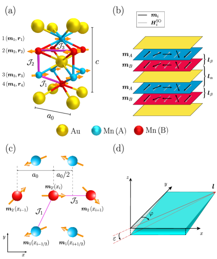
Figure 1: (a) Crystal and spin structure of the Mn₂Au tetragonal unit cell along with the types of atoms and sublattices present in the system, where the magnetic Mn-based layers are numbered and their corresponding unit magnetization vectors, $\boldsymbol{m}_{i}$, and position vectors, $\boldsymbol{r}_{i}$, are indicated. Distribution of the exchange bonds of AFM origin, $\mathcal{J}_{1}$ and $\mathcal{J}_{2}$, and the one of FM nature, $\mathcal{J}_{3}$, as well as the in-plane $xy$ basal lattice period $a_{0}$ and the out-of-plane height $c$ parameters. (b) Sketch of the distribution of the Néel-like DW magnetization, $\boldsymbol{m}_{i}$, and the SO field, $\boldsymbol{H}^{\mathrm{SO}}_{i}$, in each of the magnetic sublattices, denoted by A and B, together with the definition of two types of Néel order parameters involving different layers, $\boldsymbol{l}_{\alpha}=\left(\boldsymbol{m}_{3}-\boldsymbol{m}_{2}\right)/2$ and $\boldsymbol{l}_{\beta}=\left(\boldsymbol{m}_{1,3}-\boldsymbol{m}_{2,4}\right)/2$. (c) View from the top of the unit cell along the $z$-th spatial direction of the distribution of the first nearest neighbours of the Mn atom of layer 2 located at the position $x_{i}$ along the $x$-th axis, characterized by $\boldsymbol{m}_{2}(x_{i})$. Those neighbours of its same sublattice, at a distance $a_{0}$, are denoted by $\boldsymbol{m}_{2}(x_{i\pm 1})$, being mediated by the FM exchange interaction $\mathcal{J}_{3}$, and those from layer 1, located at an in-plane spacing $a_{0}/2$, are represented by $\boldsymbol{m}_{1}(x_{i\pm 1/2})$, and are connected through the AFM exchange contribution encoded by $\mathcal{J}_{1}$. (d) Description of the unit AFM vector, $\boldsymbol{l}=\left(\boldsymbol{m}_{\mathrm{A}}-\boldsymbol{m}_{\mathrm{B}}\right)/2$, in terms of the polar out-of-plane $\varepsilon$ and in-plane azimuthal $\varphi$ angles relative to the Cartesian coordinate system.

where the sum $\left<i,j\right>$ runs only over first nearest neighbours whose atomic positions are labeled by the indices $i,j$, being represented the unit magnetic moment in the $i$-th lattice position by $\boldsymbol{m}_{i}$. The symbols $\boldsymbol{\hat{x}}$, $\boldsymbol{\hat{y}}$, $\boldsymbol{\hat{z}}$ refer to the unit vectors along the $x$-, $y$-, and $z$-th spatial directions in the Cartesian coordinate system, while the unit vectors $\boldsymbol{\hat{u}}_{1,2}$ represent the in-plane $xy$-based directions $\boldsymbol{u}_{1}=\left[110\right]$ and $\boldsymbol{u}_{2}=\left[1\bar{1}0\right]$. Furthermore, as it can be seen in Fig. 1 (a), the lattice constant along the $x$- and $y$-th directions in the basal planes is represented by $a_{0}=3.328$ Å  while the size of the conventional unit cell along the $z$-th direction is given by $c=8.539$ Å  Khmelevskyi and Mohn (2008). Within the conventional unit cell there are two Mn atoms per each type of sublattice, A and B, giving rise to a total of four magnetic atoms. In fact, the magnetic moment of each of these Mn atoms, which coincides with the net contribution to each FM layer in the unit cell, would be given by $\mu_{\mathrm{s}}=4\mu_{\mathrm{B}}$ Barthem et al. (2013), where $\mu_{\mathrm{B}}$ is the Bohr magneton. Additionally, as it can be seen in Fig. 1 (a), there are three types of exchange contributions between magnetic moments $\boldsymbol{m}_{i}$ and $\boldsymbol{m}_{j}$ in the unit cell, which are represented by the exchange integrals $\mathcal{J}_{ij}$. This set is composed by the $\mathcal{J}_{1}$, $\mathcal{J}_{2}$, and $\mathcal{J}_{3}$ parameters, where the first two are AFM, being $\mathcal{J}_{1}=-\left(396\,\mathrm{K}\right)k_{\mathrm{B}}$ and $\mathcal{J}_{2}=-\left(532\,\mathrm{K}\right)k_{\mathrm{B}}$, and the third one is FM, being $\mathcal{J}_{3}=\left(115\,\mathrm{K}\right)k_{\mathrm{B}}$ Khmelevskyi and Mohn (2008); Barthem et al. (2013); Masrour et al. (2015), where $k_{\mathrm{B}}$ is the Boltzmann constant. On the other hand, it is possible to appreciate that there are two types of tetragonal anisotropies in the system, given by $K_{4\parallel}=1.8548\times 10^{-25}\,\mathrm{J}$ and $K_{4\perp}=2K_{4\parallel}$, and another two of uniaxial origin, denoted as $K_{2\perp}=-1.303\times 10^{-22}\,\mathrm{J}$ and $K_{2\parallel}=7K_{4\parallel}$ Shick et al. (2010); Otxoa et al. (2020a, b). The last term in Eq. (1) is the Zeeman-like contribution, where $\mu_{0}$ denotes the vacuum permeability and $\boldsymbol{H}^{\mathrm{SO}}_{i}$ expresses the staggered SO field on each $i$-th lattice site which, because the locally broken inversion symmetry occurs along the $z$-th spatial direction, is $\boldsymbol{H}^{\mathrm{SO}}_{\mathrm{A},\mathrm{B}}=\pm H^{\mathrm{SO}}_{y}\boldsymbol{\hat{y}}$ when the electric current density, $\boldsymbol{j}$, is injected along $\boldsymbol{j}\parallel\boldsymbol{\hat{x}}$, and $\boldsymbol{H}^{\mathrm{SO}}_{\mathrm{A},\mathrm{B}}=\mp H^{\mathrm{SO}}_{x}\boldsymbol{\hat{x}}$ when $\boldsymbol{j}\parallel\boldsymbol{\hat{y}}$ Železnỳ et al. (2014).

III Theoretical framework

In view of the different interactions present in the system, collected by Eq. (1), the magnetization is constrained in-plane for each Mn-based $xy$ FM layer. Thus, the type of magnetic texture that can be stabilized in each of these planes is a 1D $180^{\circ}$ Néel-like DW, as it is exposed in Fig. 1 (b). When proposing how it is possible to approach the analytical characterization of the dynamics of a 1D DW in Mn₂Au, it is worth noting that the conventional unit cell consists of four staggered magnetized layers along the $z$-th spatial direction connected through two types of AFM exchange contributions, $\mathcal{J}_{1}$ and $\mathcal{J}_{2}$, which makes it difficult to define a unique Néel order parameter in the system. However, it is feasible to reduce its characterization to a two sublattice single staggered vector-based description due to the symmetric inequivalence of the magnetic and crystallographic unit cells. To carry out this discussion, let us use the numbering of the Mn planes in accordance with Fig. 1 (a). This being the case, it is possible to differentiate two crystallographically identical Mn-based groups: one made up of planes 1 and 4, and the other by sheets 2 and 3. We note that, if an inversion transformation is carried out with respect to the unit cell center position, operation which would be characterized through their position vectors $\boldsymbol{r}_{i}$, it is possible to obtain that crystallographically the Mn atoms of plane 1 are transformed into those of the layer 4, and vice versa (this is, $\boldsymbol{r}_{1,4}\rightarrow-\boldsymbol{r}_{4,1}$). This can be extrapolated to the case of those Mn atoms that reside in the layers 2 and 3 (which would be represented by $\boldsymbol{r}_{2,3}\rightarrow-\boldsymbol{r}_{3,2}$). However, the crystallographic symmetry is not preserved if the AFM ordering of the magnetic moments in the Mn sites is taken into account because the magnetic moments that exist in the planes 1-4 and 2-3 are antiparallel with respect to each other within the exchange approximation. It is precisely this broken inversion symmetry that gives rise to the staggered SO field, $\boldsymbol{H}^{\mathrm{SO}}_{i}$, included in Eq. (1), in each type of magnetic sublattice, which allows to induce the AFM dynamics.

In this line, taking into account that Mn₂Au is a magnetically-based centro-asymmetric AFM, it is possible to introduce four vectors in the system, one FM vector, $\boldsymbol{m}_{\mathrm{a}}$, and three AFM vectors, $\boldsymbol{l}_{i}$, as linear combinations of the four sublattice magnetization vectors, $\boldsymbol{m}_{i}$, giving this as a result: $\boldsymbol{m}_{\mathrm{a}}=\left(\boldsymbol{m}_{1}+\boldsymbol{m}_{2}+\boldsymbol{m}_{3}+\boldsymbol{m}_{4}\right)/4$, $\boldsymbol{l}_{\mathrm{a}}=\left(\boldsymbol{m}_{1}-\right.$ $\left.\boldsymbol{m}_{2}-\boldsymbol{m}_{3}+\boldsymbol{m}_{4}\right)/4$, $\boldsymbol{l}_{\mathrm{b}}=\left(\boldsymbol{m}_{1}-\boldsymbol{m}_{2}+\boldsymbol{m}_{3}-\boldsymbol{m}_{4}\right)/4$, and $\boldsymbol{l}_{\mathrm{c}}=\left(\boldsymbol{m}_{1}+\boldsymbol{m}_{2}-\boldsymbol{m}_{3}-\boldsymbol{m}_{4}\right)/4$ Turov et al. (2010). In fact, one of these AFM vectors, namely $\boldsymbol{l}_{\mathrm{b}}$, can be chosen as the main one to define the system due to the specific magnetic symmetry of the Mn₂Au unit cell. At this point, we have to remember that planes 1-3 and 2-4 are magnetically identical, the relative magnetization direction being parallel to each other. Due to this, we can introduce a two sublattice model made up of Mn-based layers 2 and 3 (of type B and A represented in Fig. 1 (b), respectively) assuming that $\boldsymbol{m}_{1}=\boldsymbol{m}_{3}$ and $\boldsymbol{m}_{2}=\boldsymbol{m}_{4}$. This has a result that the AFM vectors are given now by $\boldsymbol{l}_{{\mathrm{a}},\mathrm{c}}=0$, $\boldsymbol{l}_{\mathrm{b}}=\left(\boldsymbol{m}_{3}-\boldsymbol{m}_{2}\right)/2$, while the FM vector is represented by $\boldsymbol{m}_{\mathrm{a}}=\left(\boldsymbol{m}_{3}+\boldsymbol{m}_{2}\right)/2$. This allows defining for Mn₂Au the main AFM vector as $\boldsymbol{l}_{\alpha}=\boldsymbol{l}_{\mathrm{b}}=\left(\boldsymbol{m}_{3}-\boldsymbol{m}_{2}\right)/2$ and the magnetization vector as $\boldsymbol{m}_{\alpha}=\boldsymbol{m}_{\mathrm{a}}=\left(\boldsymbol{m}_{3}+\boldsymbol{m}_{2}\right)/2$ Turov et al. (2010). In this way, it is possible to describe the dynamics in the layered AFM Mn₂Au through a two magnetic sublattice formalism taking into account only the two FM embedded layers 2 and 3, thus excluding from consideration the layers 1 and 4 for this purpose. We introduce also a more general definition of said variables in terms of the two types of magnetic layers of the system, A and B, as it is shown in Fig. 1 (b), with which we have that $\boldsymbol{l}=\left(\boldsymbol{m}_{\mathrm{A}}-\boldsymbol{m}_{\mathrm{B}}\right)/2$ and $\boldsymbol{m}=\left(\boldsymbol{m}_{\mathrm{A}}+\boldsymbol{m}_{\mathrm{B}}\right)/2$, respectively, which is consistent with the $\boldsymbol{l}_{\alpha}$ and $\boldsymbol{m}_{\alpha}$ characterization.

To address the analytical description of the system, it is necessary to evaluate how many nearest neighbours exchange-based bonds have an impact on the inhomogeneous DW transition. For this, as it can be seen in Fig. 1 (c), which shows a top view of the conventional unit cell, we will focus on the number of relevant first nearest neighbours for a Mn atom of layer 2 in an arbitrary position $x_{i}$ along the $x$-th spatial direction, which is characterized by the unit magnetization vector $\boldsymbol{m}_{2}\left(x_{i}\right)$. In this line, it is possible to observe that said atom has four intersublattice first neighbours on layer 1, at a distance $a_{0}/2$ along the $x$-th axis, which are shown through $\boldsymbol{m}_{1}(x_{i\pm 1/2})$, which are mediated by the interaction characterized by the AFM $\mathcal{J}_{1}$ parameter. Also, the aforementioned atomic position has two first intrasublattice neighbours along the $x$-th spatial direction, at a distance $a_{0}$, characterized by $\boldsymbol{m}_{2}(x_{i\pm 1})$, interacting through the FM exchange $\mathcal{J}_{3}$ contribution. It should be noted that both, the first intrasublattice neighbours in layer 2 along the $y$-th axis and the only intersublattice first nearest neighbour, mediated by the exchange interaction $\mathcal{J}_{2}$, of layer 3 along the $z$-th axis, are not taken into account because they do not impose any type of exchange penalty to determine the static or dynamic DW configuration in each of the sublattices of the system. In Suppl. Note I it can be found a simulations-based discussion about the role of the AFM exchange interaction $\mathcal{J}_{2}$ in this regard. On the other hand, due to the relative order of magnitude of the uniaxial magnetic anisotropy constants compared to the tetragonal ones, being given by $K_{2\perp}/K_{4\perp}=351$ and $K_{2\parallel}/K_{4\parallel}=7$, the fourth-order anisotropy constants will be neglected in the main approximation from now on.

In this way, we readjust the energy given by Eq. (1) for the case of a two sublattice-based description in terms of the orthogonal set of unit vectors defined by $\boldsymbol{l}$ and $\boldsymbol{m}$, which satisfy the conditions $\boldsymbol{m}^{2}+\boldsymbol{l}^{2}=1$ and $\boldsymbol{m}\cdot\boldsymbol{l}=0$. We take into account that even though these variables are constructed in terms of the magnetic sublattice types A and B, as discussed above, they refer from now on to the two FM embedded layers 2 and 3, in accordance with the definition of $\boldsymbol{m}_{\alpha}$ and $\boldsymbol{l}_{\alpha}$, the latter being explicitly represented in Fig. 1 (b). However, in our case we are interested in describing the dynamics of a single magnetic texture, which occurs entirely in a single sublattice of the system. Since the introduction of the AFM vectors $\boldsymbol{m}$ and $\boldsymbol{l}$ implicitly assumes that the motion of a single DW occurs across both magnetic sublattices, we must halve the resulting magnetic anisotropy and Zeeman-like energies. Therefore, the energy, $w$, can be rewritten, taking into account the construction of the exchange part of the energy exposed in Suppl. Note II within an effective version of the nonlinear $\sigma$-model framework Zvezdin (1979); Bar’yakhtar et al. (1985); Lifshitz and Pitaevskii (1980), due to the non-inclusion of the AFM exchange interaction along the c-axis of the system encoded by $\mathcal{J}_{2}$, in the exchange limit Papanicolaou (1995); Tveten et al. (2016), as follows

$$w=\frac{1}{2}\,A\,{\boldsymbol{m}}^{2}+\frac{1}{8}\,a\,{\left(\partial_{x}\boldsymbol{l}\right)}^{2}+w_{a}\left(\boldsymbol{l}\right)-2\gamma\hbar\,\,\boldsymbol{l}\cdot\boldsymbol{H}^{\mathrm{SO}},$$ (2)

where we introduced the homogeneous AFM exchange parameter, $A=16\absolutevalue{\mathcal{J}_{1}}$, and the inhomogeneous FM-like exchange constant, given by $a=8a^{2}_{0}\left(\mathcal{J}_{3}+\absolutevalue{\mathcal{J}_{1}}/2\right)$. Here the term $w_{a}\left(\boldsymbol{l}\right)$ encapsulates the uniaxial anisotropic contributions of the system, $w_{a}\left(\boldsymbol{l}\right)=\absolutevalue{K_{2\perp}}\,{\left(\boldsymbol{l}\cdot\boldsymbol{\hat{z}}\right)}^{2}-K_{2\parallel}\,{\left(\boldsymbol{l}\cdot\boldsymbol{\hat{y}}\right)}^{2}$, and $\partial_{x}$ expresses the variation of the order parameter along the $x$-th spatial direction. This last statement is because it has been chosen that the current is injected along $\boldsymbol{j}\parallel\boldsymbol{\hat{x}}$, so $\boldsymbol{H}^{\mathrm{SO}}=H^{\mathrm{SO}}_{y}\boldsymbol{\hat{y}}$, inducing the DW motion along the $x$-th spatial direction. Also, we have rewritten the Zeeman-like term of Eq. (1) taking into account that $\mu_{0}\mu_{s}=2\gamma\hbar$, where $\gamma$ represents the gyromagnetic ratio and $\hbar$ is the reduced Planck constant.

Along the same line, it is possible to introduce how the Landau-Lifshitz-Gilbert (LLG) equations of the magnetic sublattice magnetization motions look like in the terms of $\boldsymbol{l}$ and $\boldsymbol{m}$ vectors within the exchange limit Kosevich et al. (1990); Tveten et al. (2016), which are given by

$$\dot{\boldsymbol{l}}=\gamma\,\boldsymbol{H}^{\mathrm{eff}}_{\boldsymbol{m}}\times\boldsymbol{l},$$ (3)

$$\dot{\boldsymbol{m}}=\left(\gamma\,\boldsymbol{H}^{\mathrm{eff}}_{\boldsymbol{l}}-\alpha\,\dot{\boldsymbol{l}}\right)\times\boldsymbol{l},$$ (4)

where $\boldsymbol{H}^{\mathrm{eff}}_{\boldsymbol{l},\boldsymbol{m}}$ refers to the effective magnetic fields associated with the vector variables $\boldsymbol{l},\boldsymbol{m}$. These effective fields can be expressed as $\boldsymbol{H}^{\mathrm{eff}}_{\boldsymbol{l},\boldsymbol{m}}=-\frac{1}{2\gamma\hbar}\,\frac{\delta w}{\delta\left(\boldsymbol{l},\boldsymbol{m}\right)}$, where $\delta$ represents the functional derivative, $\alpha$ the phenomenological Gilbert damping parameter, which accounts for the dissipation processes, and the dot over a variable points out its derivative with respect to time, $t$. Through Eq. (3), it can be found that $\boldsymbol{m}=2\hbar\,\left(\dot{\boldsymbol{l}}\times\boldsymbol{l}\right)/A$, expression which can be substituted in Eq. (4) to obtain a second-order differential equation only in terms of the unit staggered AFM vector $\boldsymbol{l}$, which will be expressed by

$$\boldsymbol{l}\times\left[\left(\partial^{2}_{x}\,\boldsymbol{l}\right)-\frac{1}{v^{2}_{\mathrm{m}}}\,\ddot{\boldsymbol{l}}+\boldsymbol{h}-\frac{4}{a}\,\frac{\partial w_{a}\left(\boldsymbol{l}\right)}{\partial\boldsymbol{l}}-\eta\,\dot{\boldsymbol{l}}\right]=0,$$ (5)

where $v_{\mathrm{m}}$ represents the maximum magnon group velocity of the medium, which is given by $v_{\mathrm{m}}=\sqrt{aA}/\left(4\hbar\right)=2a_{0}\sqrt{2\absolutevalue{\mathcal{J}_{1}}\left(\mathcal{J}_{3}+\absolutevalue{\mathcal{J}_{1}}/2\right)}/\hbar=43.39$ km/s, $\boldsymbol{h}$ encodes the reduced SO field as $\boldsymbol{h}=8\gamma\hbar\,\boldsymbol{H}^{\mathrm{SO}}/a$, and $\eta$ denotes the dissipative parameter expressed as $\eta=8\alpha\hbar/a$. Interestingly, it has been predicted that an AFM exchange interaction like $\mathcal{J}_{2}$, perpendicular to the inhomogeneous DW transition, should govern the value of $v_{\mathrm{m}}$ related to the low-frequency acoustic branch, contrary to what is demonstrated in Suppl. Notes I, both within and outside of the standard nonlinear $\sigma$-model framework Zvezdin and Kostyuchenko (1999); Arana et al. (2017); Yuan et al. (2018).

In accordance with what it is shown in Fig. 1 (d), it is possible to parameterize through spherical coordinates the unit Néel order parameter taking into account which is the in-plane easy-axis direction, giving rise to $\boldsymbol{l}=\left(\sin\varphi\,\cos\varepsilon,\cos\varphi\,\cos\varepsilon,-\sin\varepsilon\right)$, where $\varphi$ represents the azimuthal angle, which accounts for the rotation of the magnetization in the $xy$ plane being measured from the $y$-th axis, while $\varepsilon$ expresses the polar angle, which describes the out-of-plane canting being characterized from the $xy$ plane. Because we are working on the exchange limit, it is possible to assume that $\varepsilon\simeq 0$, whereby the reduced AFM vector can be expressed as $\boldsymbol{l}\simeq\left(\sin\varphi,\cos\varphi,0\right)$. This being the case, it is possible to reduce Eq. (5) to a sine-Gordon wave-like equation Bar’yakhtar and Ivanov (1980); Andreev and Marchenko (1980), with the following functional form

$$\frac{1}{v^{2}_{\mathrm{m}}}\,\ddot{\varphi}-\left(\partial^{2}_{x}\varphi\right)+\frac{1}{2\Delta^{2}_{0}}\,\sin 2\varphi+h\,\sin\varphi=-\eta\,\dot{\varphi},$$ (6)

where $\Delta_{0}$ stands for the DW width at rest, which is given by $\Delta_{0}=\sqrt{a/\left(8K_{2\parallel}\right)}=a_{0}\sqrt{\left(\mathcal{J}_{3}+\absolutevalue{\mathcal{J}_{1}}/2\right)/K_{2\parallel}}=19.17$ nm, and where $h=8\gamma\hbar\,H^{\mathrm{SO}}_{y}/\,a$ denotes the reduced scalar SO field.

At this point, it is convenient to consider the magnetic texture dynamics within the framework of the well-known collective coordinates approach Rajaraman (1982). For this, it is usual to introduce what is known as Walker-like rigid profile through the angular variable that defines the spatio-temporal evolution of the magnetization, $\varphi\left(x,t\right)=2\,\arctan\,\mathrm{exp}\left[\left(x-q\left(t\right)\right)/\Delta\left(t\right)\right]$ Schryer and Walker (1974), with $q$ being the DW center position and $\Delta$ being the dynamic DW width. Due to the Lorentz invariance shown by Eqs. (5) and (6), the magnetic soliton dynamics in AFM shows emergent special relativity signatures. In particular, the DW width decreases as the velocity of the magnetic texture, $\dot{q}$, increases, which is given by the expression $\Delta\left(t\right)=\Delta_{0}\,\beta\left(t\right)$, where $\beta\left(t\right)=\sqrt{1-{\left(\dot{q}\left(t\right)/v_{\mathrm{m}}\right)}^{2}}$ represents the Lorentz factor. In order to avoid the excitation of internal modes of the magnetic texture, we focus on quasistatic processes, being its spatial extent variation governed entirely by the special relativity-based Lorentz factor, so we can neglect the time derivatives of the DW width $\Delta$. In this way, we obtain that

$$\frac{1}{\Delta\,v^{2}_{\mathrm{m}}}\,\ddot{q}+\frac{\eta}{\Delta}\,\dot{q}-h=0.$$ (7)

As it can be seen in Eq. (7), we have a Newton-like second-order differential equation for the time evolution of the DW center position, $q$, which explicitly shows the inertial nature of the magnetic texture Tveten et al. (2013); Yuan et al. (2018). In the particular case in which a constant SO field is applied, it is possible to access a steady-state-like DW motion regime after the accommodation of the soliton to its new dynamic state. In this sense, we can reduce the previous equation to a compact expression that accounts for the steady-state DW velocity, which we denote from now on as $v=\dot{q}$, which is given by

$$v=\frac{v_{\mathrm{m}}}{\sqrt{1+{\left(v_{\mathrm{m}}/v_{0}\right)}^{2}}}\,,$$ (8)

where $v_{0}=h\Delta_{0}/\eta$.

IV Relativistic and inertial domain wall dynamic signatures

To verify the predictions obtained above through our effective version of the nonlinear $\sigma$-model, we have performed atomistic spin dynamics simulations of the real crystallographic and magnetic conventional unit cell of Mn₂Au, as it is shown in Fig. 1 (a), taking into account all interactions of the system, as it is collected in Eq. (1). With this objective in mind, the system of the coupled LLG equations of motion of the local magnetic moments $\boldsymbol{m}_{i}$, being given by

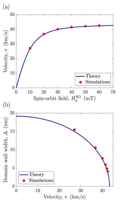
Figure 2: Comparison of the relativistic signatures for steady-state processes in Mn₂Au obtained through atomistic spin dynamics simulations and theory. (a) Saturation of the velocity, $v$, of the magnetic texture as the SO field, $H^{\mathrm{SO}}_{y}$, increases, being based the analytical formalism in Eq. (8). (b) DW width, $\Delta$, contraction as the speed $v$ of the magnetic soliton increases, the theoretical prediction coming from the combination of the relativistic expression $\Delta=\Delta_{0}\,\beta$ and Eq. (8).

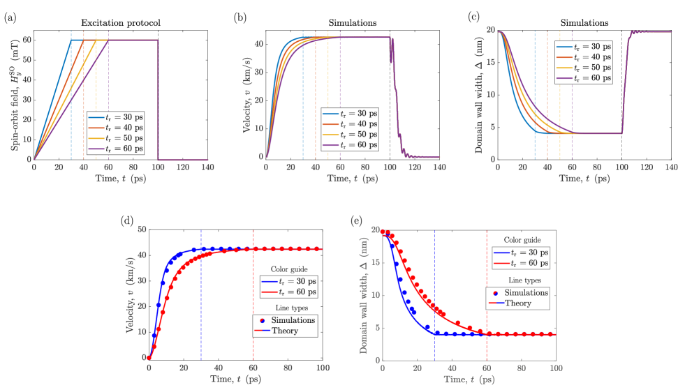
Figure 3: (a) Time-dependent staggered SO field-based excitation protocol, $H^{\mathrm{SO}}_{y}\left(t\right)$, applied in each Mn-based FM layer of Mn₂Au for different ramping times, $t_{\mathrm{r}}$. Dynamic time evolution of the DW velocity $v$ (b) and width $\Delta$ (c) obtained through atomistic spin dynamics simulations for different ramping times $t_{\mathrm{r}}$. Comparison of the dynamic time evolution of the velocity $v$ (d) and width $\Delta$ (e) of a Néel-like DW for atomistic spin dynamics simulations and the analytical expressions given by Eq. (7) and $\Delta=\Delta_{0}\,\beta$ for two ramping times, $t_{\mathrm{r}}=30$ and $60$ ps. Each vertical colored dashed line represents the end of the ramped process for the different ramping times $t_{\mathrm{r}}$, while the dashed black line denotes the instant $t=100$ ps at which the driving SO field $H^{\mathrm{SO}}_{y}$ is abruptly turned off.

$$\frac{\left(1+\alpha^{2}\right)}{\gamma}\,\dot{\boldsymbol{m}}_{i}=-\boldsymbol{m}_{i}\times\boldsymbol{H}^{\mathrm{eff}}_{i}-\alpha\,\boldsymbol{m}_{i}\times\left(\boldsymbol{m}_{i}\times\boldsymbol{H}^{\mathrm{eff}}_{i}\right),$$ (9)

is evaluated numerically site by site through a fifth-order Runge-Kutta method. Here, $\boldsymbol{H}^{\mathrm{eff}}_{i}$ represents the effective field at each lattice position, which depends on the interactions exposed in Eq. (1), as $\boldsymbol{H}^{\mathrm{eff}}_{i}=-\frac{1}{\mu_{0}\mu_{\mathrm{s}}}\frac{\delta w}{\delta\boldsymbol{m}_{i}}$, and the damping parameter is $\alpha=0.001$ Gomonay et al. (2018); Otxoa et al. (2020b, a). In this case, the computational domain consists of 60000 cells along the $x$-th propagation direction, one cell width with periodic boundary conditions along $y$-th direction, and one cell thick along the $z$-th direction cla . Due to their simple functional forms in terms of intrinsic parameters of the material, we can test the validity of our analytical formalism by comparing the values of the DW width at rest, $\Delta_{0}$, and the maximum magnon group velocity of the medium, $v_{\mathrm{m}}$, with the simulated ones. This being the case, we have found that the simulated values are $\Delta_{0}=19.78$ nm and $v_{\mathrm{m}}=43.3$ km/s. The theoretically-predicted DW width at rest $\Delta_{0}$ presents a good correspondence with the fitted rigid DW profile-based simulated value, differing only by a $3.1\%$, which possibly comes from the non-inclusion in the analytical model, for simplicity, of the in-plane tetragonal anisotropy contribution encoded by $K_{4\parallel}$. On the other hand, the maximum magnon group velocity $v_{\mathrm{m}}$ obtained analytically and by simulations coincide in a $99.93\%$. With this satisfactory correspondence between the theory and simulations, which supports the non-inclusion in our formalism of the AFM exchange interaction given by $\mathcal{J}_{2}$, we can explore the emergent special relativity signatures during steady-state DW dynamic processes. As it can be seen in Fig. 2, the saturation of the magnetic texture velocity, $v$, as it is predicted by Eq. (8), and the contraction of the DW width, $\Delta$, in correspondence with the expression $\Delta=\Delta_{0}\,\beta$, as the SO field, $H^{\mathrm{SO}}_{y}$, increases are verified.

To explore the inertial signatures on our system, we use the time-dependent SO field-based excitation regimes represented in Fig. 3 (a). As it can be seen, there are three well differentiated regions. In the first one, which covers the interval $t\in\left[\left.0,t_{\mathrm{r}}\right)\right.$, being $t_{\mathrm{r}}$ the time taken to reach a constant value of the field of $H^{\mathrm{SO}}_{y}=60$ mT, which we denote as ramping time, the rest state of the magnetic texture is disturbed through a SO field that increases linearly with time. We denote this regime as region I, and each colored dashed line in Fig. 3 corresponds to a certain $t_{\mathrm{r}}$ that defines the aforementioned domain. Consistently with Eq. (7), which implicitly shows the existence of a non-zero DW mass, the initial response of the magnetic texture to the external stimulus is fast, but not instantaneous, as it can be seen in Figs. 3 (b, c). At the time when a constant field value of $60$ mT is reached, that is, at $t=t_{\mathrm{r}}$, the magnetic soliton tends to a steady-state regime (region II), which covers the interval $t\in\left[\left.t_{\mathrm{r}},100\,\,\mathrm{ps}\right)\right.$. This upper limit is denoted by a black dashed line when appropriate in Fig. 3. Thus, it is possible to observe in Figs. 3 (b, c) that, in the region II, after a brief adaptation period to the new dynamic regime, which is a sample of the inertial nature of the process, the magnetic texture moves steadily at a speed of $v=42.56$ km/s. This is very close to the maximum magnon group velocity of the medium, denoting a $98\%$ of it, while shrinking to a width of $\Delta=4.08$ nm, which represents a contraction of $80\%$ with respect to the simulated DW width at rest. Finally, at a certain moment given by $t=100$ ps, the SO field is abruptly switched off. This makes it possible to observe that the magnetic texture is capable of initiating an after-pulse displacement in the absence of an external stimulus at the same time as its width expands until it stops completely, as it can be seen in Figs. 3 (b, c). We denote this regime as region III, and it covers the interval $t\in\left[100,140\right]$ ps.

The range of values considered for the ramping time $t_{\mathrm{r}}$ has been chosen to avoid the excitation of internal DW modes during the acceleration process, in such a way that the simulations were comparable to the scenario exposed in Section III through Eq. (7). As it can be seen in Figs. 3 (d, e), in these circumstances there is a great correspondence between the simulated and the theoretically-predicted velocity of the magnetic texture, $v$, and its spatial extent, $\Delta$, in regions I and II. However, if attention is paid to Figs. 3 (b, c) in the region III, it is possible to appreciate undulations once the SO field $H^{\mathrm{SO}}_{y}$ is turned off. These ripples observed in the simulated DW velocity and width in the region III cause longer decay times than those predicted through a simple Newton-like pseudoparticle behaviour. Therefore, we avoid the analytical evaluation of this region through Eq. (7) because the magnetic soliton is no longer fulfilling the imposed rigid profile constraint. However, the after-pulse displacement that the magnetic texture experiences in region III is related to the increase in the exchange-based relativistic DW mass obtained during the acceleration process in region I while its width shrinked. This is a purely inertial phenomenon, which is consistent with the massive pseudoparticle behavior captured by Eq. (7), in which the higher is the dynamic DW mass after turning off the external stimulus, the greater is the braking distance travelled by it. Interestingly, it is the fact that the magnetic soliton moves along a particular direction which sets how this stored relativistic exchange energy is transformed into a translational displacement, manifesting its massive particle-like behavior rather than being dissipated in a breather-like fashion or through the emission of spin waves without prolonging its mobility. For different values of the SO field during region II, we have found through simulations that there is a quasilinear relationship between the after-pulse distance travelled by the magnetic texture, $x$, normalized to the its steady-state DW width, $\Delta$, and its steady-state DW mass, $m_{\mathrm{DW}}$, normalized to its rest state value, $m^{0}_{\mathrm{DW}}$, this is, $m_{\mathrm{DW}}/m^{0}_{\mathrm{DW}}=1/\beta$ according to Eq. (7), which can be seen in Fig. 4 and can be expressed as

$$\frac{x}{\Delta}=b\,\,\frac{m_{\mathrm{DW}}}{m^{0}_{\mathrm{DW}}}+c,$$ (10)

where $b$ and $c$ are two fitting-dependent parameters, which are given, accompanied by their associated uncertainties, by $b=13.81(27)$ and $c=-13.92(89)$. It is remarkable that the DW is capable of undertaking exchange-based after-pulse displacements of the order of $4$ to $11$ times greater than the DW width at rest, $\Delta_{0}$, for SO fields between $10$-$60$ mT. This accurate prediction of the braking distance experienced by the magnetic soliton opens the door to implement low-energy consumption processes.

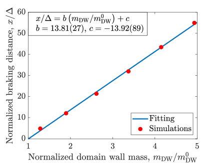
Figure 4: Quasilinear correspondence between the normalized relativistic DW mass, $m_{\mathrm{DW}}/m^{0}_{\mathrm{DW}}$, where $m_{\mathrm{DW}}$ and $m^{0}_{\mathrm{DW}}$ represent the aforementioned mass in steady-state and at rest, respectively, and the normalized braking distance, $x$, travelled by the magnetic texture once the SO field is turned off abruptly, $x/\Delta$, in terms of the steady-state DW width, $\Delta$, characterized by a linear fitting where $b$ and $c$ represent the adjustment parameters, together with their corresponding uncertainties.

V Conclusions

We addressed the theoretical characterization of the dynamic evolution of a 1D Néel-like DW in one of the FM sublattices of the layered collinear AFM Mn₂Au driven by the current-induced SO fields. Despite the complexity of the system, we have exploited the symmetric inequivalence between the crystallographic and the magnetic unit cell to reduce its description to a two-sublattice problem. Since the AFM exchange interaction directed along the c-axis of the system, which is encoded through $\mathcal{J}_{2}$, has a null projection along the 1D inhomogeneous magnetic texture transition, it has no impact on the temperature-independent standard nonlinear $\sigma$-model. Because of this, we have worked on within an effective theory framework avoiding its inclusion, methodology which can be extrapolated to layered multisublattice AFM with different exchange-oriented contributions. In the rigid profile approximation, we have shown that it is possible to reduce the dynamic description to a Newton-like second-order differential equation of motion. Comparing our formalism with atomistic spin dynamics simulations, we have been able to replicate with a high degree of precision the relativistic and inertial signatures of the magnetic texture motion during quasistatic dynamic processes within the framework of our effective model. After the abrupt shutdown of the SO field in simulations, the rigid DW profile approach is no longer supported and our analytical formalism fails to describe the after-pulse inertial dynamic regime. Interestingly, during the deceleration process the relativistic exchange energy accumulated during the previous dynamic evolution of the magnetic texture is converted into translational mobility, rather than being released in a breather-like fashion or through the emission of spin waves with non-associated displacement. We have found a quasilinear relationship that allows us to predict, for the range of simulated SO fields, the value of the braking distance travelled by the DW through the knowledge of its relativistic mass before turning off the external stimulus. This detailed dynamic characterization of the 1D magnetic texture in the complex multisublattice antiferromagnet Mn₂Au is of potential interest for AFM DW-based technology applications.

REFERENCES

- Gomonay et al. (2016) O. Gomonay, T. Jungwirth, and J. Sinova, Phys. Rev. Lett. 117, 017202 (2016).
- Shiino et al. (2016) T. Shiino, S.-H. Oh, P. M. Haney, S.-W. Lee, G. Go, B.-G. Park, and K.-J. Lee, Phys. Rev. Lett. 117, 087203 (2016).
- Yang et al. (2019) H. Yang, H. Y. Yuan, M. Yan, H. W. Zhang, and P. Yan, Phys. Rev. B 100, 024407 (2019).
- Otxoa et al. (2020a) R. M. Otxoa, P. E. Roy, R. Rama-Eiroa, J. Godinho, K. Y. Guslienko, and J. Wunderlich, Commun. Phys. 3, 190 (2020a).
- Kim et al. (2014) S. K. Kim, Y. Tserkovnyak, and O. Tchernyshyov, Phys. Rev. B 90, 104406 (2014).
- Tatara et al. (2020) G. Tatara, C. A. Akosa, and R. M. Otxoa, Phys. Rev. Res. 2, 043226 (2020).
- Tveten et al. (2013) E. G. Tveten, A. Qaiumzadeh, O. A. Tretiakov, and A. Brataas, Phys. Rev. Lett. 110, 127208 (2013).
- Yuan et al. (2018) H. Y. Yuan, W. Wang, M.-H. Yung, and X. R. Wang, Phys. Rev. B 97, 214434 (2018).
- Selzer et al. (2016) S. Selzer, U. Atxitia, U. Ritzmann, D. Hinzke, and U. Nowak, Phys. Rev. Lett. 117, 107201 (2016).
- Železnỳ et al. (2014) J. Železnỳ, H. Gao, K. Vỳbornỳ, J. Zemen, J. Mašek, A. Manchon, J. Wunderlich, J. Sinova, and T. Jungwirth, Phys. Rev. Lett. 113, 157201 (2014).
- Wadley et al. (2016) P. Wadley, B. Howells, J. Železnỳ, C. Andrews, V. Hills, R. P. Campion, V. Novák, K. Olejník, F. Maccherozzi, S. S. Dhesi, et al., Science 351, 587 (2016).
- Olejník et al. (2017) K. Olejník, V. Schuler, X. Martí, V. Novák, Z. Kašpar, P. Wadley, R. P. Campion, K. W. Edmonds, B. L. Gallagher, J. Garcés, et al., Nat. Commun. 8, 15434 (2017).
- Grzybowski et al. (2017) M. Grzybowski, P. Wadley, K. Edmonds, R. Beardsley, V. Hills, R. Campion, B. Gallagher, J. S. Chauhan, V. Novak, T. Jungwirth, et al., Phys. Rev. Lett. 118, 057701 (2017).
- Zhou et al. (2018) X. Zhou, J. Zhang, F. Li, X. Chen, G. Shi, Y. Tan, Y. Gu, M. Saleem, H. Wu, F. Pan, et al., Phys. Rev. Appl. 9, 054028 (2018).
- Bodnar et al. (2020) S. Y. Bodnar, Y. Skourski, O. Gomonay, J. Sinova, M. Kläui, and M. Jourdan, Phys. Rev. Appl. 14, 014004 (2020).
- Barthem et al. (2016) V. M. T. S. Barthem, C. V. Colin, R. Haettel, D. Dufeu, and D. Givord, J. Magn. Mat. 406, 289 (2016).
- Sapozhnik et al. (2018) A. A. Sapozhnik, M. Filianina, S. Y. Bodnar, A. Lamirand, M.-A. Mawass, Y. Skourski, H.-J. Elmers, H. Zabel, M. Kläui, and M. Jourdan, Phys. Rev. B 97, 134429 (2018).
- Kašpar et al. (2021) Z. Kašpar, M. Surỳnek, J. Zubáč, F. Krizek, V. Novák, R. P. Campion, M. S. Woernle, P. Gambardella, X. Marti, P. Němec, et al., Nat. Electr. 4, 30 (2021).
- Janda et al. (2020) T. Janda, J. Godinho, T. Ostatnicky, E. Pfitzner, G. Ulrich, A. Hoehl, S. Reimers, Z. Šobáň, T. Metzger, H. Reichlova, et al., Phys. Rev. Mat. 4, 094413 (2020).
- Otxoa et al. (2020b) R. M. Otxoa, U. Atxitia, P. E. Roy, and O. Chubykalo-Fesenko, Commun. Phys. 3, 31 (2020b).
- Yang et al. (2015) S.-H. Yang, K.-S. Ryu, and S. Parkin, Nat. Nanotechnol. 10, 221 (2015).
- Lequeux et al. (2016) S. Lequeux, J. Sampaio, V. Cros, K. Yakushiji, A. Fukushima, R. Matsumoto, H. Kubota, S. Yuasa, and J. Grollier, Sci. Rep. 6, 1 (2016).
- Luo et al. (2020) Z. Luo, A. Hrabec, T. P. Dao, G. Sala, S. Finizio, J. Feng, S. Mayr, J. Raabe, P. Gambardella, and L. J. Heyderman, Nature 579, 214 (2020).
- Shick et al. (2010) A. B. Shick, S. Khmelevskyi, O. N. Mryasov, J. Wunderlich, and T. Jungwirth, Phys. Rev. B 81, 212409 (2010).
- Barthem et al. (2013) V. M. T. S. Barthem, C. V. Colin, H. Mayaffre, M.-H. Julien, and D. Givord, Nat. Commun. 4, 2892 (2013).
- Masrour et al. (2015) R. Masrour, E. K. Hlil, M. Hamedoun, A. Benyoussef, A. Boutahar, and H. Lassri, J. Magn. Mat. 393, 600 (2015).
- Khmelevskyi and Mohn (2008) S. Khmelevskyi and P. Mohn, Appl. Phys. Lett. 93, 162503 (2008).
- Wells and Smith (1970) P. Wells and J. H. Smith, Acta Crystallogr. Sect. A 26, 379 (1970).
- Roy et al. (2016) P. E. Roy, R. M. Otxoa, and J. Wunderlich, Phys. Rev. B 94, 014439 (2016).
- Turov et al. (2010) E. A. Turov, A. V. Kolchanov, V. V. Men’shenin, I. F. Mirsaev, and V. V. Nikolaev, Symmetry and Physical Properties of Antiferromagnets (Cambridge International Science Publishing, Cambridge, 2010).
- Zvezdin (1979) A. K. Zvezdin, JETP Lett. 29, 553 (1979).
- Bar’yakhtar et al. (1985) V. G. Bar’yakhtar, B. A. Ivanov, and M. V. Chetkin, Sov. Phys. Uspekhi 28, 563 (1985).
- Lifshitz and Pitaevskii (1980) E. M. Lifshitz and L. P. Pitaevskii, Statistical Physics, Course of Theoretical Physics, Vol. 9 (Pergamon Press, Oxford, 1980).
- Papanicolaou (1995) N. Papanicolaou, Phys. Rev. B 51, 15062 (1995).
- Tveten et al. (2016) E. G. Tveten, T. Müller, J. Linder, and A. Brataas, Phys. Rev. B 93, 104408 (2016).
- Kosevich et al. (1990) A. M. Kosevich, B. A. Ivanov, and A. S. Kovalev, Phys. Rep. 194, 117 (1990).
- Zvezdin and Kostyuchenko (1999) A. K. Zvezdin and V. V. Kostyuchenko, J. Exp. Theor. Phys. 89, 734 (1999).
- Arana et al. (2017) M. Arana, F. Estrada, D. S. Maior, J. B. S. Mendes, L. E. Fernandez-Outon, W. A. A. Macedo, V. M. T. S. Barthem, D. Givord, A. Azevedo, and S. M. Rezende, Appl. Phys. Lett. 111, 192409 (2017).
- Bar’yakhtar and Ivanov (1980) I. V. Bar’yakhtar and B. A. Ivanov, Solid State Commun. 34, 545 (1980).
- Andreev and Marchenko (1980) A. F. Andreev and V. I. Marchenko, Sov. Phys. Uspekhi 23, 21 (1980).
- Rajaraman (1982) R. Rajaraman, Solitons and Instantons (North-Holland, Amsterdam, 1982).
- Schryer and Walker (1974) N. L. Schryer and L. R. Walker, J. Appl. Phys. 45, 5406 (1974).
- Gomonay et al. (2018) O. Gomonay, T. Jungwirth, and J. Sinova, Phys. Rev. B 98, 104430 (2018).
- (44) It should be noted that the absence of periodicity along the -th spatial direction in the simulated ultrathin film does not guarantee the condition used in Section III, which allowed us to reduce the system description to a two-sublattice-based nonlinear -model.