High-Accuracy Absolute Magnetometry with Application to the Fermilab Muon $g-2$ Experiment

Abstract

We present details of a high-accuracy absolute scalar magnetometer based on pulsed proton NMR. The $B$-field magnitude is determined from the precession frequency of proton spins in a cylindrical sample of water after accounting for field perturbations from probe materials, sample shape, and other corrections. Features of the design, testing procedures, and corrections necessary for qualification as an absolute scalar magnetometer are described. The device was tested at $B=1.45$ T but can be modified for a range exceeding 1–3 T. The magnetometer was used to calibrate other NMR magnetometers and measure absolute magnetic field magnitudes to an accuracy of 19 parts per billion as part of a measurement of the muon magnetic moment anomaly at Fermilab.

1 Introduction

The accurate measurement of magnetic fields is a common requirement in atomic, nuclear, and particle physics experiments. However, most experiments have a unique set of requirements on field resolution, bandwidth, spatial resolution, field magnitude and measurement range, vector versus scalar measurement, and desired accuracy. To meet differing needs, many types of magnetometers have been developed and are in broad use, including Hall sensors, fluxgate magnetometers, rotating coil, optically-pumped alkali vapor magnetometers, Faraday rotation magnetometers, magnetoresistive devices, SQUIDS, and nuclear magnetic resonance (NMR) magnetometers.

For many experiments investigating the fundamental properties of particles, atoms, or molecules in magnetic fields, high accuracy absolute scalar magnetometers are required to determine the magnitude of the magnetic induction $B\left(\vec{r},t\right)=\left|\vec{B}\left(\vec{r},t\right)\right|$ in terms of a standard such as the Tesla. Ideally, all calibrated absolute scalar magnetometers should report the same value of $B$ when inserted in the same field, regardless of the kind of magnetometer.

The highest accuracy scalar magnetometers typically use the NMR signal of a nuclear spin precessing in an external $B$ field. The spin angular precession frequency $\omega_{N}$ of a bare nucleus $N$ is directly related to the external field magnitude $B$ through the Larmor relation $\omega_{N}=\gamma_{N}B$ where $\gamma_{N}$ is the gyromagnetic ratio of the bare nuclear spin in units of radians per second per Tesla.

Since bare nuclei are difficult to work with, most practical magnetometers use nuclei shielded in an atom or molecule. One complication is that the field at the nucleus is reduced from the field to be measured by the diamagnetic shielding of the atomic electrons and other effects [1]. The reduction is directly proportional to the external field and of order 25 parts per million (ppm) for protons in molecular hydrogen or water. For shielded nuclei, the Larmor relation is modified to $\omega^{\prime}_{N}=\gamma^{\prime}_{N}B$, where the shielded gyromagnetic ratios $\gamma^{\prime}_{N}$ are typically less than the bare gyromagnetic ratios $\gamma_{N}$. Despite this complication, the gyromagnetic ratios for shielded nuclei of practical interest for magnetometers, namely protons shielded in water $\gamma^{\prime}_{p}$, and the ³He nucleus (helion) shielded in the ³He atom $\gamma^{\prime}_{h}$, are known at the level of 11 and 12 ppb respectively [2, 3, 4]. Thus in principle absolute field measurements can be made with these systems to 11–12 ppb absolute accuracy. This should be compared with the limits of other common approaches such as Hall sensors, where the proportionality constant between the Hall voltage and the external field $B$ depends on the applied Hall current and sensor properties such as electron and hole densities and mobilities. These latter factors are not easily known or stable below the ppm level, setting a limit on the absolute accuracy.

The potential for high absolute accuracy of NMR magnetometers can only be realized with careful construction and analysis of signals. For instance, the magnetization of materials used in the magnetometer construction will necessarily perturb the local field. When accuracies better than a part per million are sought, careful choice of materials and shapes is necessary to reduce this field perturbation, which must be measured. Trade-offs between absolute accuracy and resolution are also typically necessary. For instance, the RF coil used for detecting the precessing nuclear magnetic moments should be close to the NMR sample to maximize signal size and signal resolution. However, the magnetic field perturbation from the coil increases with proximity to the NMR sample, and fields from currents in the coil induced by the precessing nuclear magnetic moments, also perturbs the local field. Thus RF coil design is optimized differently for absolute magnetometry compared to magnetometers optimized for high precision. These and other design considerations, testing procedures, and corrections that should be considered for an absolute scalar magnetometer are discussed below.

1.1 Overview of the Paper

In Sec. 2, the design and performance of our calibration probe is presented. The magnetic correction terms are identified in Sec. 3. In Sec. 4, we present applications of absolute magnetometry in particle physics. The magnetic corrections for our magnetometer are quantified in Sec. 5. An extensive cross-checking program against other absolute magnetometers is discussed in Sec. 6.

2 Design and Performance

Our design choices for the absolute magnetometer (hereafter referred to as the calibration probe) are guided by the desire to minimize the magnetic perturbation of the probe on the magnetic field. A highly-symmetric construction using combinations of paramagnetic and diamagnetic materials minimize the magnetic perturbations. On the other hand, the NMR sample shape presents a non-negligible correction for $\omega_{p}^{\prime}$. Due to the difficulties associated with building an NMR sample with a spherical shape with aberrations far below the percent level, we use a cylindrical NMR sample shape since glass tubes with high symmetry are easily obtainable.

2.1 Operating Principles: Pulsed NMR

The probe is operated using pulsed NMR. When placed in an external magnetic field, proton magnetic moments build up a net polarization according to the Boltzmann distribution. A short-duration radio-frequency (RF) pulse at the resonant Larmor frequency is applied across the NMR sample using an excitation coil, generating an RF field perpendicular to the external magnetic field $\vec{B}=|B|\hat{y}$. For instance, at the magnetic field $|B|=1.45$ T used for testing this probe, the resonant frequency is 61.79 MHz. At a specific duration, the RF pulse tips the magnetization of the proton ensemble perpendicular to $\vec{B}$, known as a $\pi/2$ pulse, see Fig. 1. The proton spins then precess in the horizontal $xz$ plane and induce excitation currents in the coil due to the changing magnetic flux. The magnetization relaxes back to being aligned with $\vec{B}$, with time constant $T_{1}$. Simultaneously, spin-spin interactions and magnetic field gradients across the NMR sample cause these spins to dephase, damping out the oscillatory signal. The time over which these effects occur is known as the $T_{2}^{*}$ time, written as:

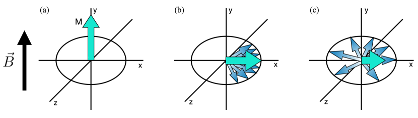
Figure 1: An illustration of the proton spin ensemble at various times relative to the $\pi/2$ pulse. The large arrow represents the magnetization $M$ of the NMR sample and the smaller arrows represent individual proton spins. Panel (a) is immediately before the $\pi/2$ pulse, panel (b) is shortly after, and panel (c) is several seconds later.

$$\frac{1}{T_{2}^{*}}=\frac{1}{T_{2}}+\frac{1}{T_{2}^{\dagger}},$$ (1)

where $T_{2}$ describes pure spin-spin interactions, and $1/T_{2}^{\dagger}\propto\gamma\Delta B$ denotes the decay time due to magnetic field gradients $\Delta B$ for an NMR sample with a gyromagnetic ratio $\gamma$. The $T_{2}^{*}$ time is necessarily less than or equal to twice the $T_{1}$ time [5, 6]. This decaying oscillatory signal is known as the free-induction decay (FID) signal.

To extract the frequencies of the probe’s FIDs, we apply a zero-crossing counting algorithm; the zero crossings and their neighboring data samples were fit to a line to determine the $i^{\text{th}}$ crossing time $t_{0}^{i}$. This in turn allows the reconstruction of the phase of the FID signal as a function of time. Fitting the phase to a seventh-order odd-polynomial [7, 8] and taking the first derivative evaluated at zero time gives the frequency of the FID. In the analysis, the baseline of the signal is treated carefully; a time-varying baseline could potentially bias the extracted frequency. We correct the baseline as follows: the algorithm first subtracts a constant baseline from the signal to center it on 0 V. The residual slope of the signal is then minimized by comparing neighboring pairs of zero crossings. We compute an iterative correction by applying the Newton-Raphson method [9] to find the roots of the residual baseline as a function of the average time difference of all pairwise zero crossings. The correction converges in about 4–5 iterations, and varied between 0 and 1 mV in magnitude. The correction had a negligible impact on the extracted frequency of the FID. The frequency analysis algorithm has been verified to be accurate to $<$1 ppb when tested against a simulation of the probe’s NMR signal. The simulation computes the voltage response of the NMR coil and accounts for its construction as well as the capacitance and inductance of the full resonant circuit (Sec. 2.2.2). The simulation also incorporates the probe’s geometry and materials, and is performed in a variety of magnetic field gradients up to 20 ppb/mm across the probe’s active volume [8].

2.2 Calibration Probe Design

2.2.1 Mechanical Construction

The design of the probe is shown in Fig. 2, and its physical assembly is given in Fig. 3. It features a near-zero magnetic susceptibility RF coil; it is a 0.97-mm outer-diameter (OD) copper tube filled with aluminum such that its effective magnetic susceptibility is 8% that of copper. The coil was wound to a length of 1 cm with 5.5 turns and 2-mm pitch. It is mounted on a $(15.065\pm 0.008)$ mm OD, $(13.470\pm 0.013)$ mm inner-diameter (ID) high-precision glass tube, with limits on concentricity of 38 $\mu$m and camber of 13 $\mu$m. This provides rigid, symmetric placement of the coil relative to the water sample, which is located at the center of the probe. We utilize an ultra-pure ASTM Type-1 water sample, housed in a $(4.9635\pm 0.0065)$ mm OD, $(4.2065\pm 0.0065)$ mm ID glass tube that has limits on concentricity of 51 $\mu$m and camber of 25 $\mu$m. The tube is held at the center of the probe via insertion into a hole in the Macor™ support on the electronics end of the probe (left side of Fig. 2). The opposite end of the water sample is held in place by a plastic adapter that slip-fits inside the 8-mm opening of the Macor™ support at the far end of the probe (right side of Fig. 2). The Macor™ parts have machining tolerances of 0.05 mm. The RF coil leads travel down opposite sides of the glass support tube, pass through 2-mm diameter holes in the Macor™ support, and are soldered to an electronics board. The outer shell of the probe is 25.4-mm OD, 1.0-mm wall aluminum alloy 2024. This shell is connected to the ground of the probe’s circuit via a copper wire, see Fig. 3.

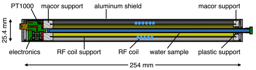
Figure 2: Design drawing for the calibration probe. Tunable capacitors and a temperature sensor are housed in the section at the far left end of the device. The straight leads of the RF coil are not drawn. Figure reproduced from Ref. [10].

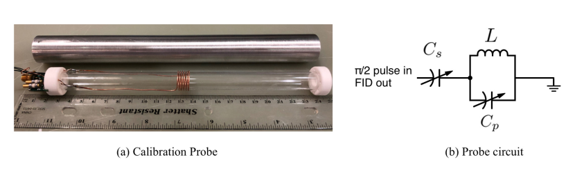
Figure 3: (a) The internal assembly of the probe with its aluminum shield. The RF coil and its leads are visible, along with the electronics board on the left. (b) A schematic depiction of the probe circuit. The series and parallel tunable capacitances $C_{s}$ and $C_{p}$, and coil inductance $L$ are indicated. The probe shell is also connected to ground (not drawn).

2.2.2 Electrical Circuitry

The RF coil, which has an inductance of 0.5 $\mu$H, is connected in parallel to a variable capacitor with a range of 1–12 pF. This LC combination is connected in series to another variable capacitor of the same range. This series capacitor is then connected in series to an SMA connector with the cable that attaches to the electronics unit that delivers the $\pi/2$ pulse and receives the FID signal (described in the following section). The physical implementation of the circuitry is shown in Fig. 3, where all components are mounted on a 22-mm wide by 18-mm long electronics PC board. A PT1000 temperature sensor is mounted on the reverse side of the board for temperature monitoring, and was determined to be in thermal equilibrium with the water sample. The PT1000 is read out over four wires by a digital multimeter (DMM). The DMM was calibrated against a precision 1 k$\Omega$ resistor, and was operated with a readout range of 10 k$\Omega$ to minimize self-heating effects. When comparing various PT1000 sensors against one another, we found the sensor stability to be better than $\pm 0.5^{\circ}$C.

2.3 NMR Data Acquisition and Readout

In order to read out the calibration probe NMR signals, we designed an NMR data acquisition system. The schematic design for the system is shown in Fig. 4. The $\pi/2$ pulse is provided by a frequency synthesizer (F1) and a 250-W amplifier (A1). This amplified signal (up to 10 W, with durations between 30–50 $\mu$s) is delivered to the NMR probe through a single-pole, double-throw RF switch (SW). The FID signal (typically 50–75 $\mu$V in amplitude) is acquired by toggling the RF switch to a pre-amplifier (A2). After amplification, this signal is band-pass filtered (BP, $(61.79\pm 2.5)$ MHz), and mixed down to $\approx$10 kHz (MX). The local oscillator signal for the mixer is provided by another frequency synthesizer (F2). Both F1 and F2 use the same clock input, a GPS-disciplined 10 MHz reference clock. The mixed-down FID is sent through additional filtering (LP1 and LP2, with cutoff frequencies of 130 kHz and 35 kHz, respectively) and amplification (OA with a gain of $\approx$28 dB). The signal amplitude is $\approx$1 V, which is digitized at 10 MHz (DG).

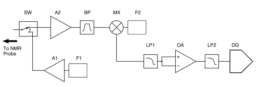
Figure 4: Signal processing schematic diagram. Item SW is an RF switch. The amplifiers are indicated by A1 and A2. Frequency synthesizer units are indicated by F1 and F2. The band-pass filter is indicated by BP and low-pass filters LP1 and LP2. The frequency mixer is indicated by MX. The operational amplifier is denoted by OA, and the digitizer is indicated by DG. For more details, see text.

In order to operate the system, we utilize a number of transistor-transistor logic pulses. These signals are obtained via a field-programmable gate array (FPGA) unit with timing precision at the nanosecond scale, exceeding our requirements of microsecond-scale timing. The pulse characteristics are managed by data acquisition software written in C++ and running on Linux.

The power required for the operation of the SW, A2, and OA components is provided by a separate power supply unit, which houses a 3.3 V, $\pm$5 V, and 12 V linear power supplies. The digitizer DG and FPGA units are powered and operated through a VME interface.

2.4 Performance

The probe has peak amplitudes of $\approx$1 V with a noise baseline of $\approx$5.5 $\mu$V/$\sqrt{\text{Hz}}$ over a bandwidth of 35 kHz for signal-to-noise ratios of $\approx$1000. A typical FID signal and its Fourier transform are shown in Fig. 5. In our test magnet facility at Argonne National Laboratory (ANL) and in-situ at Fermilab, we have achieved signal lengths of at least 400 ms, where the amplitude of the signal drops to $1/e$ of its initial maximum value.

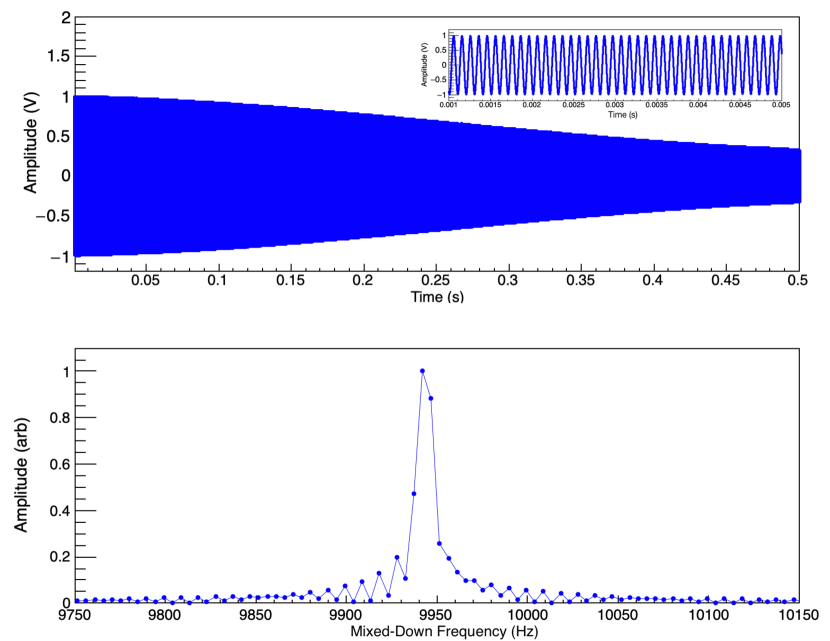
Figure 5: A typical FID recorded by the calibration probe when placed in the test magnet at ANL. Top panel: The NMR signal in the time domain; the inset shows a zoomed-in portion of the signal. Bottom panel: Fourier transform of the signal, with its spectrum normalized to its peak value. The frequency scale shown is that of the mixed-down frequency.

The testing of the probe was performed at ANL at a test solenoid facility, which uses a large-bore magnetic resonance imaging (MRI) superconducting magnet in persistent mode. In this magnet, we have achieved a frequency resolution of $\lesssim$100 parts-per-trillion (ppt) per single FID, due in part to our abilities to shim the MRI solenoid magnet to extremely high uniformity with gradients at the $\approx$1 ppb/mm level, and to measure magnetic field drifts of $\approx$9 ppb/hr. A typical data set is shown in Fig. 6. In the Fermilab Muon $g-2$ magnet, the achievable magnetic field gradients are 10–20 ppb/mm and the field stability is not as good, which reduces the single-FID frequency resolution to 10 ppb on average.

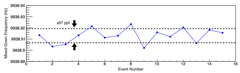
Figure 6: A typical data set showing the sensitivity of the calibration probe at ANL in the test magnet. The data acquisition system is triggered once every 5 seconds. The one-sigma band is indicated by the dashed lines, representing a standard deviation of 97 ppt.

3 Magnetic Perturbations and Their Corrections

An NMR probe is sensitive not only to the field it is immersed in, but also to the various magnetic aspects of the probe itself. This includes the NMR sample molecular structure and physical shape, and the probe material composition, geometry, and radiation damping. The magnetic field written in terms of the NMR frequency of the protons in the sample is:

$$\omega_{p}^{\prime}(T)=\omega_{p}^{\text{cp}}(T)\times\left[1+\delta^{b}\left(\text{H}_{2}\text{O},T\right)+\delta^{t}\right],$$ (2)

where $\omega_{p}^{\text{cp}}(T)$ denotes the measured frequency of the calibration probe at a temperature $T$, $\delta^{b}\left(\text{H}_{2}\text{O},T\right)$ the bulk magnetic susceptibility of water, and $\delta^{t}$ the corrections to the field due to the probe materials and other effects:

$$\delta^{t}=\delta^{s}+\delta^{p}+\delta^{\text{RD}}+\delta^{d}.$$

The quantity $\delta^{s}$ characterizes corrections due to the probe material and geometry, $\delta^{p}$ represents the correction due to paramagnetic impurities in the water sample and asymmetries in the water sample holder, $\delta^{\text{RD}}$ and $\delta^{d}$ correspond to dynamic effects relating to radiation damping and proton dipolar fields, respectively. Each of these terms will be discussed in Sec. 5.

The bulk magnetic susceptibility $\delta^{b}$ depends on the geometry and volume magnetic susceptibility of the NMR sample, given as:

$$\delta^{b}\left(\text{H}_{2}\text{O},T\right)=\left(\varepsilon-\frac{1}{3}\right)\chi\left(\text{H}_{2}\text{O},T\right),$$ (3)

where $\varepsilon$ denotes the shape factor of the NMR sample, given as $1/3$ for a perfect sphere and $1/2$ for a perfect and infinite cylinder with its long axis perpendicular to $\vec{B}$ [11]. The volume magnetic susceptibility $\chi$ for water has been parameterized based on a compilation of measurements [12]:

$$\chi\left(\text{H}_{2}\text{O},T\right)=\chi\left(\text{H}_{2}\text{O},20^{\circ}\text{C}\right)\times\left[1+a_{1}\left(T-20^{\circ}\text{C}\right)+a_{2}\left(T-20^{\circ}\text{C}\right)^{2}+a_{3}\left(T-20^{\circ}\text{C}\right)^{3}\right],$$ (4)

where $\chi\left(\text{H}_{2}\text{O},20^{\circ}\text{C}\right)=-9032\times 10^{-9}$ [13]. We assign an uncertainty of $30\times 10^{-9}$ by comparing with a measurement taken at an unknown temperature, $\chi\left(\text{H}_{2}\text{O}\right)=-9060(3)\times 10^{-9}$ [14]. The terms $a_{i}$ are $a_{1}=1.39\times 10^{-4}/^{\circ}\text{C}$, $a_{2}=-1.27\times 10^{-7}/\left({}^{\circ}\text{C}\right)^{2}$, and $a_{3}=8.09\times 10^{-10}/\left({}^{\circ}\text{C}\right)^{3}$ [12].

3.1 The Free-Proton Larmor-Precession Frequency

To extract the free proton precession frequency, there is a temperature-dependent diamagnetic shielding correction $\sigma$:

$$\omega_{p}^{\text{free}}(T)=\omega_{p}^{\prime}(T)\times\left[1+\sigma\left(\text{H}_{2}\text{O},T\right)\right],$$ (5)

where $\sigma$ takes the form:

$$\sigma\left(\text{H}_{2}\text{O},T\right)=\sigma\left(\text{H}_{2}\text{O},25^{\circ}\text{C}\right)+\frac{d\sigma\left(\text{H}_{2}\text{O}\right)}{dT}\left(25^{\circ}\text{C}-T\right).$$ (6)

The quantity $\sigma\left(\text{H}_{2}\text{O},25^{\circ}\text{C}\right)=25\text{ }691(11)\times 10^{-9}$ [15] and $d\sigma\left(\text{H}_{2}\text{O}\right)/dT=-10.36(30)\times 10^{-9}/^{\circ}\text{C}$ [16, 2, 17].

4 Applications of Absolute Magnetometry in Particle Physics

Proton NMR has been used in muonium hyperfine experiments at Los Alamos [18] and the Brookhaven National Lab (BNL) E821 Muon $g-2$ Experiment [19, 20]. This absolute magnetometer used the pulsed-NMR technique (Sec. 2.1), and featured a spherical water sample encased in a long cylindrical aluminum shield. This device achieved an accuracy of 34 ppb [21]. The leading limiting factors in its performance were the magnetic perturbation of its materials and the asphericity of the spherical glass water sample holder.

A similar magnetometer design will be used in the upcoming experiment MuSEUM at J-PARC [22], but features a cylindrical water sample [23]. This absolute magnetometer uses continuous-wave (CW) NMR and has been evaluted to be accurate to 18 ppb, where the uncertainty is dominated by the magnetic perturbations of the materials used in the magnetometer.

Absolute magnetometry is not limited to using water-based NMR samples; a ³He-based absolute magnetometer that uses pulsed NMR has been constructed recently [24, 25]. Studies presented in Ref. [25] show the ³He magnetometer agrees with the BNL E821 water-based magnetometer to within 32 ppb when placed in the same magnetic field. The uncertainty is dominated by corrections due to the materials of the ³He magnetometer.

4.1 Overview of Magnetic Field Measurements for Muon $g-2$ Experiments

NMR has been used to quantify the magnetic field in a number of muon $g-2$ experiments, including BNL E821 in the early 2000s [19, 20], the ongoing experiment at Fermi National Accelerator Laboratory (Fermilab) E989 [26], and will be used for the upcoming experiment under construction at J-PARC [27].

The magnetic moment of the positive muon is written:

$$\vec{\mu}_{\mu}=g_{\mu}\left(\frac{e}{2m_{\mu}}\right)\vec{s},$$

where $e$ denotes the electric charge of the muon, $m_{\mu}$ its mass, $\vec{s}$ its spin, and $g_{\mu}=2\left(1+a_{\mu}\right)$. The quantity $a_{\mu}$ is the muon magnetic anomaly, representing radiative corrections due to interactions of the muon with virtual fields in the quantum-mechanical vacuum. There is a 4.2$\sigma$ discrepancy between the theoretical prediction [28] and the experimental measurements [26, 20], hinting at new physics beyond the Standard Model.

The quantity $a_{\mu}$ is determined experimentally as a ratio of two angular frequencies. The intensity variation of high-energy positrons from muon decays encodes the difference between the muon spin precession and cyclotron frequencies in the magnetic field of a storage ring denoted by $\omega_{a}$. The storage ring magnetic field magnitude $B$ is measured using proton NMR and calibrated in terms of the spin precession frequency of protons shielded in a spherical water sample $\omega_{p}^{\prime}$ at a reference temperature $T_{r}=34.7^{\circ}$C. The quantity $a_{\mu}$ is extracted by combining these measurements with the quantities $\mu_{p}^{\prime}(T_{r})/\mu_{e}(H)$, $\mu_{e}(H)/\mu_{e}$, $m_{\mu}/m_{e}$ [2, 29, 3] and $g_{e}$ [30]:

$$a_{\mu}=\frac{\omega_{a}}{\tilde{\omega}_{p}^{\prime}(T_{r})}\frac{\mu_{p}^{\prime}(T_{r})}{\mu_{e}(H)}\frac{\mu_{e}(H)}{\mu_{e}}\frac{m_{\mu}}{m_{e}}\frac{g_{e}}{2},$$

where the tilde indicates that the magnetic field is weighted by the muon beam intensity distribution across the cicular cross section of the toroidal muon storage volume and averaged over the storage ring azimuthal angle.

The previous muon $g-2$ experiment (BNL E821) and the current experiment (Fermilab E989) utilize the same 14.2-m diameter superconducting storage ring magnet that produces a 1.45 T magnetic dipole field across its 18-cm gap [31]. The magnetic field around the ring is mapped using a motorized cart dubbed the “trolley” [32], which houses 17 NMR probes that contain petroleum jelly NMR samples. A single magnetic field map takes roughly 70 minutes. The muon beam is stopped every 2–3 days for this measurement. While the muon beam is circulating in the superconducting magnetic storage ring, the field is continuously monitored by “fixed” NMR probes installed in grooves machined into the walls of the main vacuum chamber above and below the muon storage region. These fixed probe measurements are tied to those of the trolley during the trolley maps, and are subsequently used to track magnetic field changes over time in the beam storage region.

To establish the absolute scale of the magnetic field seen by the trolley, a well-understood standard calibration probe is required. The magnetic characteristics of the calibration probe are measured accurately so they can be accounted for in the frequency measurements to extract the shielded precession frequency of protons in a water sample, $\omega_{p}^{\prime}$. A dedicated comparison of measurements between the standard calibration probe and the trolley in-situ at Fermilab is performed to transform trolley measurements into calibrated magnetic field maps. This program produces a correction for each trolley probe to account for the magnetic perturbation of the trolley on the field measurements [10]. For Fermilab E989, the procedure entails the in-vacuum comparison of the trolley magnetic field measurements to those of the calibration probe at a specific location in azimuth in the storage ring. As such, the calibration probe must be vacuum compatible, necessitating the use of low-outgassing materials in the probe construction (see Sec. 2).

The level of precision achieved for the magnetic field calibration in BNL E821 was 90 ppb [20], with a separate 50 ppb attributed to the calibration probe [21]. The total uncertainty budget for the magnetic field measurements in E989 is 70 ppb, with 35 ppb allotted to the calibration probe [33]. We have designed, built, and deployed a calibration probe in Fermilab E989 with an accuracy of 15 ppb.

5 Magnetic Characteristics of the High-Accuracy Calibration Probe

The magnetic characteristics of the calibration probe affect the field experienced by the protons in the water sample. The correction $\delta^{t}$ associated with this must be quantified to high precision in order to accurately extract the shielded proton Larmor frequency $\omega_{p}^{\prime}$. The magnetic effects are categorized into intrinstic and configuration-specific terms, discussed in detail in the following subsections.

5.1 Intrinsic Effects

Intrinsic effects relate to the perturbation of the external magnetic field due to the presence of the probe materials, quantified as a correction $\delta^{s}$, the impurity of the water sample, $\delta^{p}$, the shape of the water sample, $\delta^{b}$, and dynamic effects including radiation damping $\delta^{\text{RD}}$ and magnetic fields from the precessing proton spins $\delta^{d}$. In the following we quantify each term.

5.1.1 Material Effects

Material effects enter due to the magnetization of all materials surrounding the NMR sample. For a perfectly symmetric probe, perturbations arise as the square of the magnetic susceptibility and are much smaller than 1 ppb. However, the probe is not perfectly symmetric; we therefore quantify the material correction $\delta^{s}$ as:

$$\delta^{s}\left(\theta_{\text{roll}},\theta_{\text{pitch}}\right)=\delta^{\text{roll}}\left(\theta_{\text{roll}}\right)+\delta^{\text{pitch}}\left(\theta_{\text{pitch}}\right),$$ (7)

where $\delta^{\text{roll}}$ denotes the correction due to the probe materials dependent upon the probe’s roll angle $\theta_{\text{roll}}$; that is, how the probe is oriented about its long axis relative to the magnetic field axis. The term $\delta^{\text{pitch}}$ represents the correction for effects due to the angular orientation $\theta_{\text{pitch}}$ of the probe relative to the magnetic field axis. These angles are defined in Fig. 7.

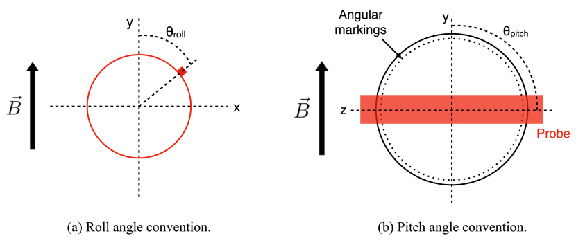
Figure 7: (a) End view of the calibration probe, illustrating the roll angle for material perturbation studies. The roll angle is the angle between the ground screw of the probe (filled square) and the magnetic field axis. (b) Top-down view of the setup used for determining the material perturbation due to the pitch angle of the calibration probe. The probe is mounted on a rotational stage using small pieces of double-sided tape (not shown). The dotted markings indicate the angular position of the probe axis. Drawing is not to scale.

The quantity $\delta^{s}$ was determined by comparing measurements inside the calibration probe with a fixed test probe and with the calibration probe removed. The calibration probe was constructed specifically so that a test probe can fit inside it. The test probe was mounted on a rigid stand and locked to a single location in the magnet with a repeatability of $<$1 mm. This ensures that uncertainties due to coupling between 1 ppb/mm field gradients and alignment errors are limited to be less than 1 ppb. Figure 8 shows the typical setup. Three sets of measurements with and without the calibration probe were used to correct for linear magnetic field drift in time [34]. The net change with and without the calibration probe is the correction $\delta^{s}$.

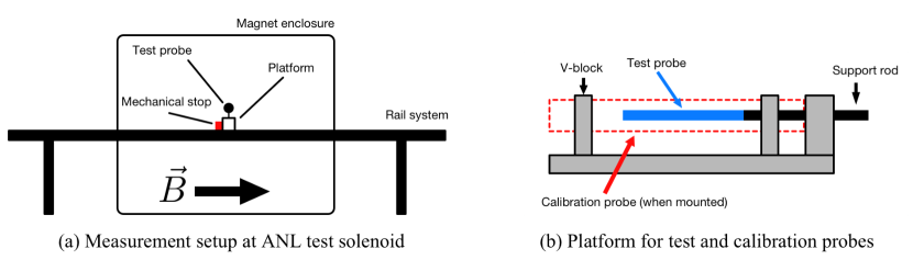
Figure 8: The setup for measuring $\delta^{s}$ for the calibration probe at ANL. (a) The test probe (long axis coming out of the page) is mounted on a retractable platform and secured by a mechanical stop for repeatability of the setup. (b) A side view of the platform on which the test probe is mounted. The dotted red rectangle indicates the calibration probe position when mounted on the platform, such that the test probe is inside the calibration probe. The test probe and calibration probe active volumes are aligned.

To quantify $\delta^{s}$ as a function of the probe’s roll angle $\theta_{\text{roll}}$, we took measurements of the magnetic field of the test solenoid at ANL with the test probe inserted in the calibration probe (c.f., Fig. 8). We compared magnetic field measurements when rotating the calibration probe 0^∘, $\ldots$, 315^∘ in steps of 45^∘, see Fig. 9. The roll angle of 0^∘ is defined such that the grounding screw of the probe is parallel to the magnetic field. Overall, we found that the test probe field measurements vary between $-2.4$ ppb and 19.5 ppb, depending on the roll angle of the calibration probe. The data are well described by a simple symmetrical form:

$$f\left(\theta_{r}\right)=p_{0}+p_{1}\left[3\cos^{2}\left(\theta_{r}+p_{2}\right)-1\right],$$

where $p_{i}$ are determined from the fit to the data. In particular, we find $\delta^{s}(0,0)=(-1.4\pm 4.0)$ ppb.

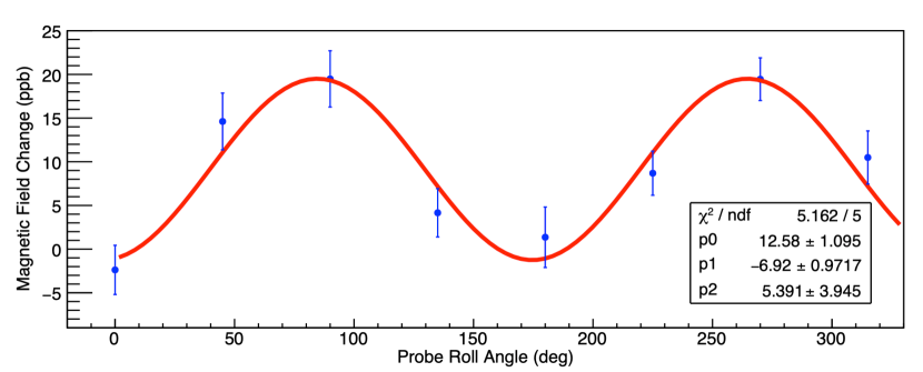
Figure 9: The results of the measured change in the field (in parts per billion) seen by the test probe when the roll angle of the calibration probe is changed. The error bars represent the uncorrelated uncertaintes of the measurements. The red curve represents the fit described in the text.

We must also consider the pitch angle $\theta_{\text{pitch}}$ of the calibration probe relative to the external magnetic field axis. To assess this effect, we mounted the probe on a rotational stage that allows for angular rotation of the probe as illustrated in Fig. 7. We performed measurements with the probe oriented at angles of 2.5^∘ and 5^∘ relative to its nominal orientation perpendicular to the magnetic field. The field as measured by the calibration probe was lower by ($16.2\pm 2.5$) ppb for the 2.5^∘ orientation, and lower by ($50\pm 1$) ppb for the 5^∘ orientation.

The results of the studies above are used in Sec. 5.2 to quantify the perturbations of the calibration probe when installed at Fermilab.

5.1.2 Bulk Magnetic Susceptibility

Possible asymmetries and field perturbations due to the water sample geometry affect the bulk magnetic susceptibility $\delta^{b}$ (Eq. (3)). To evaluate this term and its uncertainty, we examine the shape factor.

The length of the water NMR sample also has an effect on the magnetic field; if the sample were an infinitely long cylinder, then no perturbation due to edge effects would be present. However, the water sample has a finite length $L=\left(228.6\pm 1.0\right)$ mm, with a diameter $D=(4.2065\pm 0.0065)$ mm. To quantify how much the geometry of the sample affects the magnetic field, we evaluate the shape factor $\varepsilon$ characterizing the NMR sample magnetization as a surface integral [35]. Due to the symmetry of the NMR sample and its alignment relative to the magnetic field, the quantity $\varepsilon$ can be expressed as:

$$\varepsilon\approx\frac{1}{2}\frac{1}{\sqrt{1+4R^{2}/L^{2}}}.$$ (8)

Evaluating this expression using the values stated above for $L$ and $D=2R$, we find $\varepsilon=0.499\text{ }915\text{ }37(26)$. The uncertainty is dominated by the uncertainty of the long length $L$ with a sub-dominant contribution from the diameter $D$ of the sample tube.

To confirm the magnetic perturbation due to our water sample length, we took a series of measurements retracting the water sample from its seated position in the probe by 5 mm, compared to measurements with the water sample fully inserted in the probe. We found that the field as measured by the calibration probe increases by $(0.2\pm 0.2)$ ppb. This is consistent with the change in the field expected from evaluating $\varepsilon$ using Eq. (8) for a length $L$ shorter by 5 mm compared to using the nominal value for $\varepsilon$ when inserted into the bulk magnetic susceptibility $\delta^{b}$ (Eq. (3)).

To determine the uncertainty on $\delta^{b}$, we combine the uncertainties on the water magnetic susceptibility $\chi$ (Eq. (4)) and the uncertainty on $\varepsilon$ to obtain an uncertainty of 6.0 ppb. The magnitude of $\delta^{b}$ will change with temperature; evaluating Eq. (3) at $T=25^{\circ}$C, we determine $\delta^{b}=(-1505.6\pm 6.0)$ ppb.

5.1.3 Water Sample

While we utilize an ASTM Type-1 ultra-pure water sample in a highly-symmetric glass tube, we need to quantify any magnetic impurities or imperfections that can manifest as perturbations to our magnetic field measurements. These are encapsulated in the term $\delta^{p}$, given as:

$$\delta^{p}=\delta^{\text{O}_{2}}+\delta^{w}+\delta^{c},$$

where $\delta^{\text{O}_{2}}$ denotes the correction due to dissolved oxygen in the water sample; $\delta^{w}$ accounts for how much the measured field changes due to a water sample obtained from a different vendor; $\delta^{c}$ quantifies the correction due to the camber of the water sample tube (c.f., Sec. 2.2.1).

Oxygen is paramagnetic, and thus can perturb the magnetic field if it is dissolved in the NMR sample. We directly measure this effect by preparing a water sample that has been boiled to remove any dissolved oxygen, effectively degassing it. The preparation consisted of heating both the sample tube and the water so that when the water was poured into the tube using a syringe, the glass would not shatter. We then performed field measurements with the nominal sample with no special preparation and the degassed sample, swapping the two samples back and forth. We measured a total of three trials, where a trial consists of a measurement with the nominal sample and the degassed sample. We find $\delta^{\text{O}_{2}}=(1.4\pm 1.0)$ ppb. This result is consistent with expectations. An approximate dissolved oxygen concentration at 25^∘C of 8.2 mg/L corresponds to a number density $N=1.55\times 10^{17}$ cm^-3 in water. The volume susceptibility is roughly $\chi_{\text{O}_{2}}=4\pi N(g_{e}\mu_{B})^{2}(S(S+1))/3k_{B}T\approx 1.2\times 10^{-8}$ where $S=1$ for oxygen [5]. This suggests a correction to the shape-dependent bulk susceptibility of $(1/6)\times\chi_{\text{O}_{2}}\approx 2\times 10^{-9}$.

For the term $\delta^{w}$, we studied the change in the NMR frequency when comparing water samples from different vendors. For this test, we prepare two NMR water samples from different vendors and use different glass tubes for each sample. We measure the magnetic field using the calibration probe and each of the prepared NMR water samples, and repeat this process for a total of three trials. We find $\delta^{w}=(-0.4\pm 1.4)$ ppb.

We did not measure the magnetic perturbation of the water sample glass tube. This is negligible if the tube is infinitely long and perfectly symmetric (i.e., concentric construction with no camber). However, the water sample tube has finite length and non-zero camber (c.f., Sec. 2.2.1), and so we estimate the correction $\delta^{c}$. We considered how much the measured frequency depends on the roll angle of the water sample by taking consecutive measurements using the calibration probe. We rotated the water sample by 90^∘ for each measurement for a total sample rotation of 360^∘. Across all measurements, we found that the measured field changed by 1 ppb, leading to a correction $\delta^{c}=(-1\pm 1)$ ppb.

Combining the terms $\delta^{\text{O}_{2}}$, $\delta^{w}$, and $\delta^{c}$ together in quadrature, we determined $\delta^{p}=(0\pm 2)$ ppb.

5.1.4 Radiation Damping

Radiation damping arises when the current induced in the RF coil due to the precessing proton spins produces its own RF magnetic field that acts to rotate the spins back to being pointed along the external magnetic field, artificially reducing the length of the signal. This phenomenon is proportional to the relative difference of the resonant frequency of the probe $f_{0}$ and the Larmor frequency $f_{L}$ of the proton spins. Radiation damping is also dependent on the $z$ component of the magnetization of the NMR sample as a function of time $M_{z}(t)$ [36]. To estimate the magnitude of the radiation damping effect, we considered the calibration probe’s sensitivity to its tune and the sensitivity to the change in $M_{z}$.

To assess how much the magnetic field measurement depends on the probe tune, we measured the magnetic field at the nominal tune of the ANL test solenoid magnetic field, and compared that to a measurement where we detune the probe using its on-board capacitors by $\approx$100 kHz. We find no systematic shift larger than 1 ppb.

We estimated the contribution from the proton spin magnetization $M_{z}(t)$ by varying the $\pi/2$ pulse duration and observed how the extracted frequency changed. We found the effect to be less than 2 ppb over a large range of RF pulse durations from 5–50 $\mu$s.

For a conservative estimate, we combine the calibration probe’s sensitivity to the RF pulse duration and the resonant tune in quadrature to find a correction factor $\delta^{\text{RD}}=(0\pm 3)$ ppb.

5.1.5 Proton Dipolar Field

Dipolar coupling of spins of distant molecules in the NMR sample can produce a non-zero contribution to the measured magnetic field and must be evaluated. We estimate the contribution by considering a coupling of a given proton spin to a classical dipolar magnetic field due to the other protons as described in Ref. [37]. We also approximate the effect as a modification of the molecular electrons’ magnetizations, which changes the bulk magnetic susceptibility of oxygen (c.f., Eq. (3)). We found the two calculations to be consistent with one another and assigned a correction $\delta^{d}=\left(0\pm 2.5\right)$ ppb.

5.2 Effects Specific to the Muon $g-2$ Experiment at Fermilab

There are perturbations unique to the configuration at Fermilab when the probe was installed in-situ for the calibration program with the trolley system. Figure 10 shows the configuration at Fermilab. The probe was mounted on a 0.8-m long rod affixed to a 3-dimensional translation stage, which allows aligning the calibration probe’s sensitive volume to overlap with the trolley probes’ sensitive volumes. With this setup, Eq. (7) has to be modified to:

$$\delta^{s,\text{config}}=\delta^{s}(0,0)+\delta^{\text{mag}}+\delta^{\text{roll}}+\delta^{\text{pitch}}+\delta^{\text{cable}}+\delta^{\text{vac}}+\delta^{T},$$ (9)

where we use $\delta^{s}(0,0)$ (Eq. (7)) since the probe is installed at Fermilab with $\theta_{\text{roll}}=\theta_{\text{pitch}}\approx 0^{\circ}$; $\delta^{\text{mag}}$ is the correction due to magnetic images of the probe induced in the $g-2$ magnet pole pieces; $\delta^{\text{roll}}$ denotes the correction due to a non-zero roll angle of the probe; $\delta^{\text{pitch}}$ is due to a non-zero pitch angle of the probe; $\delta^{\text{cable}}$ denotes the correction due to the SMA cable that delivers the $\pi/2$ signal and receives the FID signal; $\delta^{\text{vac}}$ denotes the correction factor to account for measurements being performed in air as opposed to in vacuum. In the following, we address each term. Note that $\delta^{s}(0,0)$ and $\delta^{\text{mag}}$ have been evaluated together as a single term, see Sec. 5.2.1.

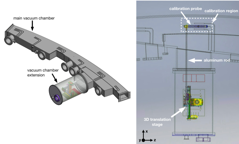
Figure 10: The assembly of the calibration probe on its 3-dimensional translation stage system at Fermilab. Left: Assembly with respect to the main vacuum chamber of the experiment. Right: Top-down, wireframe view of the assembly. The magnetic field axis is pointed along the $y$ axis.

5.2.1 Magnetic Images

When the probe is placed in the magnetic storage ring at Fermilab, it induces magnetic images in the upper and lower pole pieces, see Fig. 11. To determine the correction due to the calibration probe materials and magnetic images, $\delta^{s}(0,0)+\delta^{\text{mag}}$, we need to evaluate the correction for the probe oriented with the roll and pitch angle of $0^{\circ}$ inside the muon storage ring magnet. We accomplish this by measuring the image effect at ANL in the test solenoid. To check our results, we also measured the effect in-situ at Fermilab.

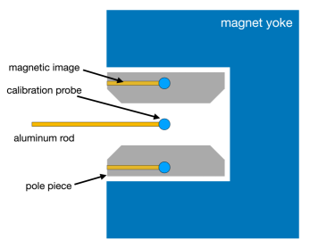
Figure 11: An illustration of magnetic images of the calibration probe and its aluminum rod in the steel pole pieces of the Muon $g-2$ storage ring magnet.

To measure the magnetic image effect in the test solenoid at ANL, we measured the change in the magnetic field seen by a test probe with and without the presence of the calibration probe placed one image distance (18 cm) away. We performed six trials of test probe readings with and without the calibration probe placed at its image location. We find the calibration probe increases the test probe magnetic field reading by $(3.0\pm 2.7)$ ppb. In the Muon $g-2$ magnet, there is a magnetic image above and below the calibration probe location; by symmetry, this doubles the magnitude of the measured effect at ANL, resulting in a magnetic image of $(6.0\pm 5.4)$ ppb. The measured value of the probe material perturbation for $\theta_{\text{roll}}=\theta_{\text{pitch}}=0^{\circ}$ is $\delta^{s}(0,0)=(-1.4\pm 4.0)$ ppb (Sec. 5.1.1). The perturbation of the adapter was measured separately to be $(-8.0\pm 3.5)$ ppb. Combining these terms together, we determine the correction $\delta^{s}(0,0)+\delta^{\text{mag}}=\left(3.4\pm 7.6\right)$ ppb.

The general setup at Fermilab is shown in Fig. 12. The measurements were performed at the center of the magnet gap using the same procedure discussed in Sec. 5.1.1. This procedure was repeated for 8 pairs of measurements with the calibration probe installed and not installed on the stage. To correct for field drift, we stationed the trolley roughly 124 cm downstream in azimuth in the storage ring to take data simultaneously with our test probe measurements. Averaging over all trials, we find good agreement with the value measured at ANL. The magnetically noisier environment at Fermilab makes it very difficult to obtain results with uncertainties smaller than 8 ppb.

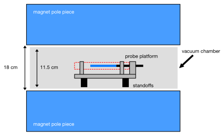
Figure 12: The setup at Fermilab for the measurement of the magnetic images of the calibration probe induced in the magnet pole pieces. The dotted red rectangle indicates the calibration probe position when mounted. The probe’s adapter that connects it to its support rod was included in this study (not drawn). The pole-pole separation of 18 cm is indicated. The vacuum chamber that fits in between the pole pieces is represented by the large light gray band between the magnet pole pieces. The clearance into this enclosure is roughly 11.5 cm. Drawing is not to scale.

To build confidence in our measurements, we also calculate the magnetic images of the probe and its support rod numerically. The magnetic image of an object in a nearby material with relative magnetic permeability $\mu_{r}$ is written [38]:

$$\Delta B^{\prime}\approx\left(\frac{\mu_{r}-1}{\mu_{r}+1}\right)\Delta B\left(x,y,z^{\prime}\right)\approx\Delta B\left(x,y,z^{\prime}\right).$$

This approximation follows because $\mu_{r}=1450$ for the ultra-pure magnet steel at 1.45 T [31]. As such, to evaluate the magnetic image of the material, we compute the magnetic perturbation of the calibration probe at a vertical height $z^{\prime}$ that describes the distance from the probe active volume to the image location in a given pole piece. This calculation is performed for both the upper and lower pole piece, where the calibration probe is located at the center of the magnet gap. To determine the magnetic image of the probe, we compute the magnetic image of each component of the probe, following:

$$\Delta\vec{B}\left(\vec{r}\right)=\int_{V}d^{3}\vec{r}\,^{\prime}\left[\frac{3\left[\vec{m}\left(\vec{r}\,^{\prime}\right)\cdot\left(\vec{r}-\vec{r}\,^{\prime}\right)\right]\left(\vec{r}-\vec{r}\,^{\prime}\right)}{|\vec{r}-\vec{r}\,^{\prime}|^{5}}-\frac{\vec{m}\left(\vec{r}\,^{\prime}\right)}{|\vec{r}-\vec{r}\,^{\prime}|^{3}}\right],$$ (10)

where the magnetic moment $d\vec{m}=\chi\vec{B}_{\text{ext}}\left(\vec{r}\,^{\prime}\right)dV$ for a given material. We sum over all materials in the probe, including its adapter that connects the probe to the support rod; we do not include the effect due to the water and its glass tube, which we estimate to be small. The computed effect is consistent with our measurements at ANL.

We evaluate the magnetic perturbation and image of the calibration probe support rod separately because of its very different geometry compared to the calibration probe. We did not make a measurement at ANL since the rod is too large to fit into the test magnet; due to the magnetically-noisy environment at Fermilab, measurements were difficult to perform. Following the same general prescription above, we compute $\left(\delta^{s}(0,0)+\delta^{\text{mag}}\right)_{\text{calc}}^{\text{rod}}=\left(8.0\pm 5.0\right)$ ppb. We used the commercial software OPERA for finite-element calculations of the magnetic field to account for the field falloff near the pole piece edges.

To evaluate the term $\delta^{s}(0,0)+\delta^{\text{mag}}$ for the calibration probe and support rod, we combine the measurement at ANL for the probe and the calculation for the support rod and find $\delta^{s}(0,0)+\delta^{\text{mag}}=\left(11.4\pm 9.0\right)$ ppb.

5.2.2 Probe Roll Angle

As discussed in Sec. 5.1.1, the probe roll angle may change the size of the correction; as such, we must use a specific value from our measurements based on what the roll angle is in the installed setup at Fermilab. The probe is installed such that its ground screw (see Fig. 3) is pointed along the magnetic field, and we have measured the roll angle of the probe to be $\ll$1^∘ under the roll angle convention adopted for the study. Therefore, we give a conservative estimate of the effect due to this asymmetry to be $\delta^{\text{roll}}=(0\pm 1)$ ppb based on our results in Sec. 5.1.1.

5.2.3 Probe Pitch Angle

The pitch of the calibration probe when installed in-situ at Fermilab was measured to be 0.68^∘. We therefore make a conservative estimate that the pitch angle acts to reduce the field by $\delta^{\text{pitch}}=(4.4\pm 4.4)$ ppb, where we linearly scale down the value measured at the 2.5^∘ angle at ANL (Sec. 5.1.1).

5.2.4 SMA Cable

The magnetic properties of the SMA cable that connects to the probe must also be considered. We measured its perturbation in the ANL test solenoid by placing the SMA connector roughly 12.7 cm from the active volume of our test probe. We maintain the same distance and relative orientation between the SMA connector and the active volume of the calibraton probe. Comparing field measurements with the cable set up and with it removed, we find that the field is lowered due to the presence of the cable. The corresponding correction value is $\delta^{\text{cable}}=(1.4\pm 3.0)$ ppb.

5.2.5 Vacuum Effect

When the studies in Secs. 5.1.1 and 5.2.1 were conducted, the results effectively describe the field perturbation of the calibration probe relative to an equivalent calibration probe made of air. In the Muon $g-2$ Experiment, the perturbation of the calibration probe must be known in a vacuum environment.

To evaluate this effect, we compute the perturbation (Eq. 10) for a hypothetical calibration probe that has a magnetic susceptibility defined as $\chi^{\prime}=\chi-0.2\chi_{\text{O}_{2}}$, where $\chi_{\text{O}_{2}}$ is the magnetic susceptibility of oxygen. We find that the perturbation of the probe turns out to be 2 ppb smaller when evaluating Eq. (10) using $\chi^{\prime}$ for each material. In the Muon $g-2$ analysis, we account for this using a correction $\delta^{\text{vac}}=\left(-2\pm 2\right)$ ppb. This correction is accounted for in our calculation of the magnetic perturbation and image effect in Sec. 5.2.1.

5.2.6 Temperature Effect

When extracting the shielded proton precession frequency from NMR measurements, we account for the temperature dependence of the diamagnetic shielding of water (c.f., Eq. (6)). As such, the stability of our temperature readout is considered. The stability of 0.5^∘C as described in Sec. 2 results in a temperature correction $\delta^{T}=(0\pm 5)$ ppb.

5.2.7 Summary of Probe Perturbations and Uncertainties at Fermilab

The results of the studies above are given in Table 1. The material correction of the probe in-situ at Fermilab has been measured to be:

$$\delta^{s,\text{config}}=\delta^{s}(0,0)+\delta^{\text{mag}}+\delta^{\text{roll}}+\delta^{\text{pitch}}+\delta^{\text{cable}}+\delta^{\text{vac}}+\delta^{T}=(15.2\pm 12.0)\text{ ppb}.$$

Table 1: The calibration probe magnetic corrections due to the probe materials and other effects specific to the setup at Fermilab. The total uncertainty in the final row is the quadrature sum of each uncertainty.

Source	Symbol	Magnitude (ppb)	Uncertainty (ppb)
Material + Images	$\delta^{s}(0,0)+\delta^{\text{mag}}$	$11.4$	$9.0$
Roll Angle	$\delta^{\text{roll}}(\theta_{\text{roll}}=0^{\circ})$	$0$	$1$
Pitch Angle	$\delta^{\text{pitch}}(\theta_{\text{pitch}}=0.68^{\circ})$	$4.4$	$4.4$
SMA Cable	$\delta^{\text{cable}}$	$1.4$	$3.0$
Vacuum Effect	$\delta^{\text{vac}}$	$-2$	$2$
Water Sample Temperature	$\delta^{T}$	$0$	$5$
Total Material Correction	$\delta^{s,\text{config}}$	$15.2$	$12.0$

This includes effects due to the probe’s SMA cable and its support rod. We additionally account for the presence of oxygen in our measurements.

For the Muon $g-2$ Experiment, the probe’s magnetic corrections sum to (at $T=25^{\circ}$C):

$$\delta^{t,\text{config}}=\delta^{s,\text{config}}+\delta^{p}+\delta^{\text{RD}}+\delta^{d}=(15.2\pm 12.7)\text{ ppb}.$$

The correction due to water sample paramagnetic impurities is $\delta^{p}=(0\pm 2)$ ppb (Sec. 5.1.3). The radiation damping term is estimated to be $\delta^{\text{RD}}=(0\pm 3)$ ppb (Sec. 5.1.4), while the contributions to the dipole field due to the precessing protons in the water are estimated as $\delta^{d}=(0\pm 2.5)$ ppb (Sec. 5.1.5). These numbers are summarized in Table 2. Combining the uncertainty on the probe total correction $\delta^{t,\text{config}}$ with that of the bulk magnetic susceptibility $\delta^{b}$, the calibration probe is accurate to 15 ppb in extracting the shielded proton frequency $\omega_{p}^{\prime}$ for the Muon $g-2$ Experiment at Fermilab.

Table 2: The calibration probe magnetic corrections due to intrinsic properties $\delta^{p}$, $\delta^{\text{RD}}$, and $\delta^{d}$, and configuration-specific effects $\delta^{s,\text{config}}$ relevant to the Muon $g-2$ Experiment at Fermilab. The contribution from the bulk magnetic susceptibility $\delta^{b}$ is also listed and evaluated at 25^∘C. The last row shows the total correction, $\delta^{b}+\delta^{t,\text{config}}$, evaluated at 25^∘C.

Source	Symbol	Magnitude (ppb)	Uncertainty (ppb)
Material Correction (Fermilab)	$\delta^{s,\text{config}}$	$15.2$	$12.0$
Water Impurity	$\delta^{p}$	$0$	$2$
Radiation Damping	$\delta^{\text{RD}}$	0	$3$
Proton Dipolar Field	$\delta^{d}$	0	$2.5$
Bulk Magnetic Susceptibility	$\delta^{b}\left(\text{H}_{2}\text{O},T=25^{\circ}\text{C}\right)$	$-1505.6$	$6.0$
Total Correction	—	$-1490.4$	$14.1$

6 Cross Checks

In addition to quantifying the various correction terms $\delta$ for the calibration probe, we have performed extensive cross-checks against other calibration standards used for muon $g-2$ experiments; in particular, the E821 spherical water probe [21], the newly-constructed ³He probe [24, 25], and a water-based continuous-wave (CW) NMR probe to be used for the future J-PARC muon $g-2$ experiment [23]. All cross-check measurements were performed in the test magnet at ANL.

6.1 Comparison to E821

We performed a direct comparison against the E821 probe, using a platform similar to the one shown in Fig. 8. The calibration probe was placed on the stage and measured the magnetic field at the center of the solenoid; the E821 probe was swapped into the same location and the measurement for that probe was also performed. We conducted three pairs of measurements. The measured difference between the spherical (E821) and cylindrical (calibration) probes was $\delta^{b}_{\text{sph.}-\text{cyl.}}=(1514\pm 15)$ ppb, where the uncertainty is dominated by the asphericity of the E821 water sample. This difference is in agreement with Eq. (3), which gives 1506 ppb for the water magnetic susecptibility $\chi\left(\text{H}_{2}\text{O},T=25^{\circ}\text{C}\right)=-9038\times 10^{-9}$ and the shape factor $\varepsilon=1/3$ for a perfect sphere and 1/2 for an infinite cylinder with its long axis perpendicular to $\vec{B}$.

6.2 Comparison to ³He

The cross check against the ³He probe is sensitive to very different systematic effects due to the very different probe constructions and different NMR samples. A similar measurement scheme to the one presented in the previous section was used to compare the ³He and E821 probes. This work is described in Ref. [24]. After applying corrections for the material perturbations of the E821 probe and ³He probe, and correcting the E821 probe to $T=25^{\circ}$C, the ratio of the ³He to the E821 probe frequencies was measured to be $0.761\text{ }786\text{ }139(29)$ (38 ppb). This agrees with a previous measurement of the ratio of frequencies from ³He and water in a spherical sample, $0.761\text{ }786\text{ }1313(33)$ (4.3 ppb) [4]. This result indirectly calibrates the calibration probe to the ³He probe via the E821 probe; the calibration probe is validated to $(10\pm 38)$ ppb.

6.3 Comparison to the J-PARC Calibration Probe

The magnetic field team at J-PARC has built a water-based CW-NMR probe [23] for the future muon $g-2$ experiment at J-PARC [22]. We have undertaken an extensive cross-calibration program comparing our pulsed NMR probe with their CW NMR probe. While both probes have similar construction materials and geometries, the NMR measurement approach is very different, and thus sensitive to different systematic effects. The cross-calibration program was carried out at $|\vec{B}|=1.45$ T and 1.7 T, where we have constructed an additional calibration probe to function at 1.7 T. The analysis of the data from that program is ongoing. A future cross-calibration program is planned at 3 T, for which we have constructed a calibration probe.

7 Conclusion

We have presented the design, performance, and magnetic characteristics and their associated uncertainties for a highly accurate water-based NMR calibration magnetometer. The probe has demonstrated a single-FID resolution of better than 100 ppt in a highly-uniform test solenoid at ANL; in-situ at Fermilab, the probe has a resolution of 10 ppb.

The probe’s intrinsic magnetic characteristics $\delta^{s}$, $\delta^{p}$, $\delta^{\text{RD}}$, and $\delta^{d}$ were studied and quantified. In the probe’s deployment in the Muon $g-2$ Experiment at Fermilab to calibrate the trolley probe magnetic field measurements, configuration-specific perturbations $\delta^{s,\text{config}}$ were quantified. The probe was found to be accurate to 15 ppb in extracting the shielded-proton Larmor precession frequency $\omega_{p}^{\prime}$ from the NMR magnetic field measurements, exceeding the 35 ppb goal for the experiment.

We have performed a careful validation program comparing the calibration probe to the E821 probe and to a novel ³He-based probe that has been recently developed. We found excellent agreement with the BNL probe after accounting for Eq. (3), and via an indirect approach, found agreement with the ³He probe at the $(10\pm 38)$ ppb level.

The absolute magnitude of the magnetic field may be extracted using the calibration probe when accounting for the water diamagnetic shielding term $\sigma$. Incorporating the uncertainty on $\sigma$ of 11 ppb [15], the calibration probe is accurate with a precision of 18.6 ppb in determining the free-proton Larmor precession frequency from water NMR measurements.

8 Acknowledgements

We would like to thank our colleague K. Sasaki for many useful discussions, and R. Reimann for carefully reading the manuscript and providing helpful comments. We gratefully acknowledge the engineering and technical support received at both Argonne National Lab and Fermilab in the process of building the probe and executing the various measurement programs. This work is supported by the U.S. Department of Energy, Office of High Energy Physics under contracts DE-FG02-88ER40415 (University of Massachusetts), DE-AC02-06CH11357 (Argonne National Laboratory), and DE-FG02-97ER41020 (University of Washington), Department of Energy, Office of Nuclear Physics under contract DE-AC05-06OR23177 (Thomas Jefferson National Accelerator Facility), and NSF grant PHY-1812314 (University of Michigan).

Appendix A Component Listings

In this section we provide tables of the various components and their corresponding manufacturer and part number details. Table 3 contains the parts for the calibration probe and Tables 4 and 5 contains the parts used in the data acquisition system.

Table 3: Components in the NMR calibration probe.

Part	Manufacturer	Model	Link
RF coil	Doty Scientific™	90179	https://dotynmr.com
15-mm OD glass tube	Wilmad LabGlass™	515-7PP-9	https://customglassparts.com
5-mm OD glass tube	Wilmad LabGlass™	507-PP-9	https://customglassparts.com
Water sample	Cole Parmer™	8005496	https://coleparmer.com/i/labchem-water-deionized-acs-grade-astm-type-i-1-l/8005496
Capacitors	Knowles Voltronics™	NMA1J12HVS	https://www.digikey.com/en/products/detail/knowles-voltronics/NMA1J12HVS/6362741
Temperature sensor	TE Connectivity™	NB-PTCO-165	https://www.te.com/usa-en/product-NB-PTCO-165.html

Table 4: Components in the NMR data acquistion system. The column Diagram Label refers to those in Fig. 4.

Diagram Label	Manufacturer	Model	Link
F1 and F2	Stanford Research Systems™	SG380	https://www.thinksrs.com/products/sg380.html
A1	Tomco™	BT00250-Gamma	https://www.everythingrf.com/products/microwave-rf-amplifiers/tomco-technologies/567-503-bt00250-gamma
SW	Mini-Circuits™	ZSW2-63DR+	https://www.minicircuits.com/WebStore/dashboard.html?model=ZSW2-63DR%2B
A2	Pasternack™	15A1013	https://www.pasternack.com/50-db-gain-1000-mhz-low-noise-high-gain-amplifier-sma-pe15a1013-p.aspx
BP	Lark Engineering™	Custom	https://www.bench.com/lark
MX	Mini-Circuits™	ZAD-3H+	https://www.minicircuits.com/WebStore/dashboard.html?model=ZAD-3H%2B
LP1 and LP2	KR Electronics™	Custom	http://www.krelectronics.com
OA	Analog Devices™	AD797	https://www.analog.com/en/products/ad797.html
DG	Struck Innovative Systeme™	SIS3316	https://www.struck.de/sis3316.html

Table 5: Additional components in the NMR data acquisition system. Also included are the power supplies used in the power supply unit. These items are not shown in Fig. 4.

Part	Manufacturer	Model	Link
FPGA	Acromag™	IP-EP201	https://www.acromag.com/shop/embedded-i-o-processing-solutions/pcie-products/pcie-carrier-boards/mezzanine-i-o-modules-for-pcie-carriers/fpga-i-o-support-for-pcie-carriers/ip-ep200-cyclone-ii-fpga-with-digital-i-o-jtag-configured/?attribute_part-number=IP-EP201%3A+48+TTL+bidirectional+I%2FO
VME crate	Wiener™	6U VME 6023	https://www.wiener-d.com/product/6u-vme64x-6023-full-size-chassis/
Digital multimeter	Keithley™	2100	https://www.tek.com/en/products/keithley/digital-multimeter/2100-series
3.3 V power supply	Acopian™		https://www.acopian.com/single-l-screw-m.html
$\pm$5 V power supply	Bel Power Solutions™	HAA5-1.5/OVP-AG	https://belfuse.com/product/part-details?partn=HAA5-1.5/OVP-AG
12 V power supply	Bel Power Solutions™	HB12-1.7-AG	https://belfuse.com/product/part-details?partn=HB12-1.7-AG

References

- [1] N. F. Ramsey, Magnetic shielding of nuclei in molecules, Phys. Rev. 78 (1950) 699.
- [2] W. D. Phillips, W. E. Cooke and D. Kleppner, Magnetic Moment of the Proton in H2O in Bohr Magnetons, Metrologia 13 (1977) 179.
- [3] E. Tiesinga, P. J. Mohr, D. B. Newell and B. N. Taylor, “The 2018 CODATA recommended values of the fundamental physical constants (Web Version 8.1).” \urlhttps://physics.nist.gov/cuu/Constants/.
- [4] J. L. Flowers, B. W. Petley and M. G. Richards, A measurement of the nuclear magnetic moment of the helium-3 atom in terms of that of the proton, Metrologia 30 (1993) 75.
- [5] A. Abragam, Principles of Nuclear Magnetism. Oxford University Press, 1961.
- [6] D. D. Traficante, Relaxation. Can , be longer than ?, Concepts in Magnetic Resonance 3 (1991) 171.
- [7] B. Cowan, Asymmetric NMR lineshapes and precision magnetometry, Meas. Sci. Technol. 7 (1996) 690.
- [8] R. Hong et al., Systematic and Statistical Uncertainties of the Hilbert-Transform Based High-precision FID Frequency Extraction Method, J. Mag. Res. 329 (Aug, 2021) 107020 [physics.ins-det/2101.08412].
- [9] J. Raphson, Analysis Æequationum Universalis. London: Thomas Bradyll, 2 ed., 1697, https://doi.org/10.3931/e-rara-13516.
- [10] T. Albahri et al., Magnetic-field measurement and analysis for the Muon g-2 Experiment at Fermilab, Phys. Rev. A 103 (2021) 042208 [hep-ex/2104.03201].
- [11] J. A. Osborn, Demagnetizing factors of the general ellipsoid, Phys. Rev. 67 (1945) 351.
- [12] J. S. Philo and J. M. Fairbank, Temperature dependence of the diamagnetism of water, J. Chem. Phys. 72 (1980) 4429.
- [13] J. F. Schenck, The role of magnetic susceptibility in magnetic resonance imaging: MRI magnetic compatibility of the first and second kinds, Med. Phys. 23 (1996) 815.
- [14] B. H. Blott and G. J. Daniell, The determination of magnetic moments of extended samples in a SQUID magnetometer, Meas. Sci. Technol. 4 (1993) 462.
- [15] P. J. Mohr, B. N. Taylor and D. B. Newell, CODATA Recommended Values of the Fundamental Physical Constants: 2010, Rev. Mod. Phys. 84 (2012) 1527 [physics.atom-ph/1203.5425].
- [16] B. W. Petley and R. W. Donaldson, The temperature dependence of the diamagnetic shielding correction for proton NMR in water, Metrologia 20 (1984) 81.
- [17] Y. I. Neronov and N. N. Seregin, Precision determination of the difference in shielding by protons in water and hydrogen and an estimate of the absolute shielding by protons in water, Metrologia 51 (2014) 54.
- [18] W. Liu et al., High Precision Measurements of the Ground State Hyperfine Structure Interval of Muonium and of the Muon magnetic moment, Phys. Rev. Lett. 82 (1999) 711.
- [19] G. W. Bennett et al., Measurement of the Negative Muon Anomalous Magnetic Moment to 0.7 ppm, Phys. Rev. Lett. 92 (2004) 161802 [hep-ex/0401008].
- [20] G. W. Bennett et al., Final Report of the Muon E821 Anomalous Magnetic Moment Measurement at BNL, Phys. Rev. D 73 (2006) 072003 [hep-ex/0602035].
- [21] X. Fei, V. W. Hughes and R. Prigl, Precision measurement of the magnetic field in terms of the free-proton NMR frequency, Nucl. Instrum. Meth. A 394 (1997) 349.
- [22] MuSEUM collaboration, H. A. Torii et al., Precise Measurement of Muonium HFS at J-PARC MUSE, JPS Conf. Proc. 8 (2015) 025018.
- [23] H. Yamaguchi et al., Development of a CW-NMR Probe for Precise Measurement of Absolute Magnetic Field, IEEE Trans. Appl. Supercond. 29 (2019) 9000904.
- [24] M. Farooq, Absolute Magnetometry with 3He: Cross Calibration with Protons in Water. PhD thesis, University of Michigan, 2019.
- [25] M. Farooq, T. Chupp, J. Grange, A. Tewsley-Booth, D. Flay, D. Kawall et al., Absolute Magnetometry with He3, Phys. Rev. Lett. 124 (2020) 223001.
- [26] B. Abi et al., Measurement of the Positive Muon Anomalous Magnetic Moment to 0.46 ppm, Phys. Rev. Lett. 126 (2021) 141801 [hep-ex/2104.03281].
- [27] M. Abe et al., A New Approach for Measuring the Muon Anomalous Magnetic Moment and Electric Dipole Moment, physics.ins-det/1901.03047.
- [28] T. Aoyama et al., The anomalous magnetic moment of the muon in the Standard Model, Phys. Rep. 887 (2020) 1.
- [29] W. Liu, M. G. Boshier, S. Dhawan, O. van Dyck, P. Egan, X. Fei et al., High precision measurements of the ground state hyperfine structure interval of muonium and of the muon magnetic moment, Phys. Rev. Lett. 82 (1999) 711.
- [30] D. Hanneke, S. Fogwell Hoogerheide and G. Gabrielse, Cavity control of a single-electron quantum cyclotron: Measuring the electron magnetic moment, Phys. Rev. A 83 (2011) 052122.
- [31] G. T. Danby et al., The Brookhaven muon storage ring magnet, Nucl. Instrum. Meth. A 457 (2001) 151.
- [32] S. Corrodi, P. D. Lurgio, D. Flay, J. Grange, R. Hong, D. Kawall et al., Design and performance of an in-vacuum, magnetic field mapping system for the muon g-2 experiment, JINST 15 (2020) P11008.
- [33] J. Grange et al., Muon (g-2) Technical Design Report, physics.ins-det/1501.06858.
- [34] E. Swanson and S. Schlamminger, Removal of zero-point drift from AB data and the statistical cost, Meas. Sci. Technol. 21 (2010) 115104.
- [35] R. E. Hoffman, Measurement of magnetic susceptibility and calculation of shape factor of NMR samples, J. Mag. Res. 178 (2006) 237.
- [36] A. Vlassenbroek, J. Jeener and P. Broekaert, Radiation damping in high resolution liquid NMR: A simulation study, J. Chem. Phys. 103 (1995) 5886.
- [37] J. Jeener, A. Vlassenbroek and P. Broekaert, Unified derivation of the dipolar field and relaxation terms in the Bloch-Redfield equations of liquid NMR, J. Chem. Phys. 103 (1995) 1309.
- [38] J. D. Jackson, Classical Electrodynamics. John Wiley and Sons, 3 ed., 1999.