Cluster Assembly Times as a Cosmological Test

Abstract

The abundance of galaxy clusters in the low-redshift universe provides an important cosmological test, constraining a product of the initial amplitude of fluctuations and the amount by which they have grown since early times. The degeneracy of the test with respect to these two factors remains a limitation of abundance studies. Clusters will have different mean assembly times, however, depending on the relative importance of initial fluctuation amplitude and subsequent growth. Thus, structural probes of cluster age such as concentration, shape or substructure may provide a new cosmological test that breaks the main degeneracy in number counts. We review analytic predictions for how mean assembly time should depend on cosmological parameters, and test these predictions using cosmological simulations. Given the overall sensitivity expected, we estimate the cosmological parameter constraints that could be derived from the cluster catalogues of forthcoming surveys such as Euclid, the Nancy Grace Roman Space Telescope, eROSITA, or CMB-S4. We show that by considering the structural properties of their cluster samples, such surveys could easily achieve errors of $\Delta\sigma_{8}=0.01$ or better.

1 Introduction

The ‘concordance’ $\Lambda$-Cold Dark Matter ($\Lambda$CDM) cosmological model is now well established as a single theoretical framework that is consistent with many different observational tests. The present-day abundance of dark matter and dark energy and the statistical properties of the matter distribution are increasingly well constrained, as expressed by cosmological parameters with gradually decreasing uncertainties (e.g. Planck Collaboration et al., 2020). As the uncertainties in parameter values shrink; however, they reveal tension in several places in the model. Most notably, the Hubble parameter $H_{0}$ appears to differ significantly between high-redshift and low-redshift tests, with the tension in independent measurements of this parameter now exceeding $4\sigma$ (Riess et al. 2019; see Verde et al. 2019 for a review). In addition to the $H_{0}$ tension, there is also growing evidence that the amplitude of the matter fluctuations (typically expressed as $\sigma_{8}$, the r.m.s. of fluctuations in the matter density on a scale of $8h^{-1}$Mpc) may display a similar tension at the 2–3$\sigma$ level (or $\sim 0.1$ in this parameter, e.g. Battye et al., 2015; Douspis et al., 2019; To et al., 2021; Heymans et al., 2021). More generally, the fundamental natures of dark energy and dark matter remain unknown, raising the possibility of new, exotic physics not yet included in the standard cosmological model.

Given the evidence for tension in the current results, multiple, independent tests of the standard cosmological model are needed, on different mass and length scales and at different redshifts, to either reconcile the current results, or to reveal the physical origin of the disagreements. Current and forthcoming space missions, including Euclid, the Nancy Grace Roman Space Telescope (Roman), and eROSITA (Pillepich et al., 2012), together with data from large ground-based surveys such as UNIONS (Chambers et al., 2020), DESI (DESI Collaboration et al., 2016) or Rubin LSST (LSST Science Collaboration et al., 2009), or experiments such as CMB-S4 (Abazajian et al., 2019), will provide remarkable new datasets, mapping out structure over a significant fraction of the observable universe, out to redshifts of a few. Given, on the one hand, the enormous potential of this data, and, on the other hand, the exacting precision required to resolve current parameter tensions, there is a need for new tests of the cosmological model that make full use of our growing understanding of structure formation.

The measured abundance of massive galaxy clusters is a classic cosmological test. Cluster abundance has been estimated using samples detected in the X-ray (e.g. Henry et al., 2009; Mantz et al., 2010; Böhringer et al., 2014), via the Sunyaev-Zel’dovich (SZ) effect (e.g. de Haan et al., 2016; Planck Collaboration et al., 2020), in optical galaxy redshift surveys (e.g. Abdullah et al., 2020), in weak lensing surveys (Kacprzak et al., 2016), or using combinations of these techniques (e.g. Abbott et al., 2020; Costanzi et al., 2021). These rare objects evolve from peaks in the matter distribution present at early times, and their present-day abundance places a tight constraint on the function $S=\sigma_{8}\Omega_{\rm m}^{\gamma}$, where $\Omega_{\rm m}$ is the present-day matter density parameter, and $\gamma\approx 0.5$ is the growth index. Cluster abundance measurements alone do not place very tight constraints on $\Omega_{\rm m}$ or $\sigma_{8}$ individually, due to the degeneracy between them. Simply counting clusters does not leverage the full potential of the underlying datasets, however. The structural properties of clusters — their projected shape, central concentration, substructure and non-axisymmetry — are all related to their degree of dynamical relaxation, which in turn traces their formation history (see Taylor, 2011, for a review). Thus, measurements of these properties provide a separate constraint on the growth rate. While measurements of structural parameters in individual clusters may be noisy, the sheer number of systems expected in forthcoming surveys should allow us to make robust measurements of the average trends, using the expertise developed in fields like weak lensing.

The idea of using the structural properties of clusters to constrain cosmological parameters is not new (e.g. Richstone et al., 1992; Evrard et al., 1993; Mohr et al., 1995), but the context for these tests has changed radically in the 30 years since the idea was first proposed. First, the size of the datasets has grown enormously, giving better statistics. Second, our understanding of the systematics in individual structural measurements has developed considerably. Third, there is increasing sophistication in understanding and exploiting large, complex datasets. In particular, fields such as cosmic shear have illustrated how it is possible to extract parameter constraints from large sets of noisy measurements, even when the link between parameters and observables is indirect and non-linear. Finally, simulations of structure formation have progressed dramatically, allowing us to calibrate some aspects of non-linear structure formation at the per cent level, even if other aspects remain uncertain. Thus, it seems high time to reconsider cosmological tests based on the internal structure of haloes.

In this paper, we consider the possibility of estimating from their structural properties the mean assembly time or formation epoch for a large sample of galaxy clusters. This measurement of mean ‘age’ would leverage the same data already collected for cluster abundance studies, providing an independent constraint on the cosmological parameters. We focus in particular on the parametric dependence of halo age, and its sensitivity to the parameters $\Omega_{\rm m}$ and $\sigma_{8}$; in a subsequent paper, we will consider the (non-trivial) path to developing practical observational tests based on age estimates. The outline of the paper is as follows. In Section 2, we review theoretical models of cluster abundance and age, and use them to predict how these properties vary as a function of the cosmological parameters. Given the approximate nature of the theoretical estimates, in Section 3 we test these predictions using catalogues from several different N-body simulations. We show that with some careful analysis, we can reconcile the analytic and numerical results to reasonable accuracy. In Section 4, we estimate the sensitivity a realistic observational program could achieve, using concentration as a proxy for age. Finally, in Section 5, we review and summarize our results. The details of the analytic calculations and the dependence of several important quantities on the cosmological parameters are discussed in the appendices. We consider a range of cosmologies throughout the paper, but assume flatness ($\Omega_{\rm m}+\Omega_{\Lambda}=1$), and take a model with $\Omega_{\rm m}=0.3$ as the fiducial case.

2 Cosmological Sensitivity of Halo Abundance and Halo Age

We will begin by estimating the potential sensitivity of age tests, using theoretical predictions of how cluster abundance and age depend on the cosmological parameters. We use analytic models of abundance and age based on the extended Press & Schechter formalism, and calculated using standard tools and techniques summarized in Appendix A.

2.1 Analytic Models of the Halo Mass Function

The Press–Schechter (PS – Press & Schechter, 1974; Bond et al., 1991) and extended Press–Schechter (EPS – Lacey & Cole, 1993) formalisms provide a convenient analytic framework for computing the number density of dark matter haloes and their growth rate, given a background cosmological model. The basic expression for the halo mass function, derived assuming spherical collapse, is

$$n(M)dM=\sqrt{\frac{2}{\pi}}\frac{\rho_{0}}{M}\frac{\delta_{c}}{\sigma^{2}}\exp\left(-\frac{\delta_{c}^{2}}{2\sigma^{2}}\right)\left|\frac{d\sigma}{dM}\right|dM\,,$$ (1)

where $\rho_{0}$ is the matter density at the redshift of interest, $\sigma=\sigma(M)$ is the r.m.s. amplitude of fluctuations in the density field smoothed on mass scale $M$, and $\delta_{c}$ is the threshold for collapse to a virialized halo. Although fluctuations grow in amplitude as $z$ decreases to zero, the condition for collapse by redshift $z$ can also be considered at some fixed, early redshift, taking $\sigma(M)$ to be a function of mass only, and $\delta_{c}=\delta_{c}(z)$ to be a function of the collapse redshift.

The mass function can also be written in a more compact form as

$$n(M,t)dM=\frac{\rho_{0}}{M}f_{PS}(\nu)\left|\frac{d\nu}{dM}\right|dM\,,$$ (2)

where $\nu(M,z)\equiv\delta_{c}(z)/\sigma(M)$ is the height of the collapse threshold at redshift $z$, relative to typical fluctuations on mass scale $M$, and

$$f_{\rm PS}(\nu)=\sqrt{\frac{2}{\pi}}\exp\left(-\frac{\nu^{2}}{2}\right)$$ (3)

is the mass fraction that has collapsed per unit interval of $\nu$.

It is well known, however, that this basic form of the mass function fails to reproduce the halo abundance found in N-body simulations, particularly for low-mass haloes (Sheth & Tormen, 1999, 2002; Jenkins et al., 2001). This failure is due to several simplifying assumptions made in the model, the most important one being a fixed threshold for (spherical) collapse $\delta_{c}$ that is independent of mass and environment. To solve this problem, Sheth & Tormen (1999, ST hereafter) considered a mass-dependent collapse threshold (or ‘moving barrier’), to derive a functional form that better fits the mass function from simulations

$$f_{ST}(\nu)=A\sqrt{\frac{2a}{\pi}}\left(1+\frac{1}{\left(\sqrt{a}\nu\right)^{2p}}\right)\exp\left(-\frac{a\nu^{2}}{2}\right)\,,$$ (4)

with $A=0.322$, $a=0.707$ and $p=0.3$.

A number of subsequent studies have improved our understanding of the mass function. Tinker et al. (2008) demonstrated that the HMF is not completely universal, but evolves with redshift; allowing the parameters $A$, $a$, and $p$ in the fit to evolve as a power-law of $1+z$ provides a better match to simulations. This non-universality has since been confirmed by other groups (e.g. Watson et al., 2013). Despali et al. (2016), argued that it is in fact, an artifact of the halo mass definition, and that the common choices of overdensity of 200 or 178 times the critical density induce much of the non-universality. Finally, several authors (Velliscig et al., 2014; Bocquet et al., 2016; Castro et al., 2021) have studied the impact of baryonic effects on the HMF by measuring halo masses, profiles, and abundance in hydrodynamic simulations. These improvements to the HMF fit are required in precision applications, but are generally secondary in importance ($\leq 20$% – Tinker et al. 2008; Velliscig et al. 2014; Bocquet et al. 2020), relative to the large variations in abundance with cosmology shown below. Thus, for simplicity in what follows, we will assume the ST form of the collapsed fraction (Eq. 4), in order to study how abundance and age depend on cosmology. We discuss the possible effect of baryons on the internal structure of haloes in Section 4.4 below.

2.2 Cosmological Dependence of Halo Abundance

Cluster abundance depends on the cosmological parameters both through the cluster mass function and through the survey volume. Within a survey volume subtending a solid angle $\Delta\Omega$, the expected number of clusters in the mass bin $i$: $[M^{i},M^{i+1}]$ and redshift bin $j$: $[z_{j},z_{j+1}]$ is

$$N(M_{i},z_{j})=\frac{\Delta\Omega}{4\pi}\int_{z_{j}}^{z_{j+1}}dz\frac{dV}{dz}\int_{M_{i}}^{M_{i+1}}\frac{dn}{dM}\,dM\,,$$ (5)

where $dn/dM$ is the HMF given above and $dV/dz$ is the volume element per unit solid angle and per unit redshift. As discussed previously, the HMF is calculated as a fraction of the material in a region that has collapsed to form haloes on some mass scale. Thus, rather than relating the halo abundance to the volume probed by the survey, we can express it in terms of the total mass $M_{V}$ of material in the survey volume:

$$N(M_{i},z_{j})=\frac{\Delta\Omega}{4\pi}\int_{z_{j}}^{z_{j+1}}dz\frac{dM_{V}}{dz}\int_{M_{i}}^{M_{i+1}}f(\nu)\frac{d\nu}{dM}dM\,.$$ (6)

The advantage of this form is that we can now separate the cosmological dependence of the first factor, the total mass $M_{V}$ probed by the survey in a given redshift range $\Delta z$, from that of the second factor, which is the fraction $f(\nu)\Delta\nu$ of that mass that has collapsed to form haloes in the mass range $\Delta\nu=(d\nu/dM)\Delta M$ by that redshift.

To make explicit the cosmological dependence of the HMF, in Appendices B and C we consider each of these factors separately. Over a realistic range of ($\Omega_{\rm m}$, $\sigma_{8}$), the survey mass $M_{V}$ varies by a factor of $\lesssim 2$, while the collapsed fraction can vary by several orders of magnitude, and thus dominates the parametric dependence of the HMF.

As demonstrated in Appendix C, the peak height $\nu$ varies approximately as $\nu(M,z)\propto(\sigma_{8})^{-1}\Omega_{\rm m}^{\alpha(z)}\Omega_{\rm m}^{-\beta(M)}\,$. The resulting behaviour in the $\Omega_{\rm m}$–$\sigma_{8}$ plane is shown in Fig. 1, for several mass/redshift combinations. We see that peak height depends mainly on $\sigma_{8}$; variations in $\Omega_{\rm m}$ introduce a slight tilt in the contours, that goes from negative at low mass/redshift, where $\beta(M)>\alpha(z)$, to slightly positive at high mass/redshift (and low $\Omega_{\rm m}$), where $\alpha(z)>\beta(M)$ (see also Appendix C, and the lower right panel of Fig. 12, which shows the dependence on $\Omega_{\rm m}$ for fixed $\sigma_{8}$, at several different masses and redshifts).

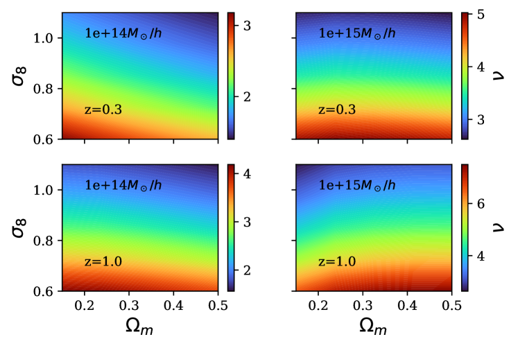
Figure 1: Variation of the peak height $\nu$, for a halo of the mass and redshift indicated, in the $\Omega_{\rm m}$–$\sigma_{8}$ plane.

In both spherical collapse (PS – Eq. 3) and ellipsoidal collapse (ST – Eq. 4) models, the collapsed fraction exhibits power-law growth for $\nu<1$, and an exponential decay for $\nu>1$. Thus, there are two main regimes, the first where the abundance of haloes increases with $\nu$, and the second where it decreases rapidly. The effect of the cosmological parameters on the two regimes is shown, for instance, in Fig. 14. The amplitude of fluctuations $\sigma_{8}$ controls the mass at which the transition between regimes occurs, while $\Omega_{\rm m}$ controls the sharpness of the transition. In the case of clusters, we are generally in the second regime, where increases in $\nu$ produce an exponential decrease in abundance. Thus, the parametric dependence of the collapsed fraction (shown in the right panel of Fig. 11) is very similar to the corresponding figure for peak height, Fig. 1, but with an inverted and logarithmic colour scale, since $f(\nu)\propto\exp(-\nu^{2}/2)$ implies that in a log scale, $\ln(f)\propto-\nu^{2}/2$.

Finally, we can combine the parametric dependence of the survey volume and the collapsed fraction (shown in the left and right panels of Fig. 11 respectively) to plot the dependence of number counts on $\Omega_{\rm m}$ and $\sigma_{8}$. This is shown in Fig. 2, for the same mass/redshift combinations considered previously. We note that the variation of the total mass within the survey volume has a minimal effect, and aside from the change in the overall scale, the contours are almost identical to those for the collapsed fraction.

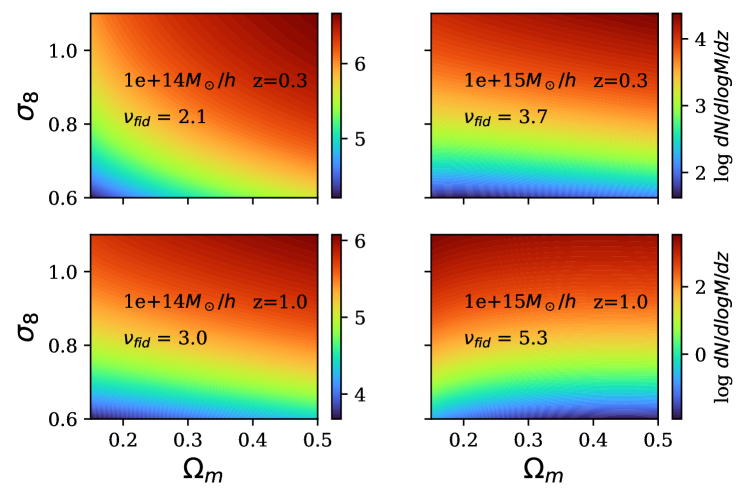
Figure 2: The cosmological dependence of the differential cluster number counts, per unit log mass and per unit redshift. The colour scale is logarithmic. The value of the peak height at different masses and redshifts for our fiducial cosmology ($\Omega_{m}=0.3$, $\sigma_{8}=0.8$) is shown to illustrate the dependence of the contour shapes on peak height.

2.3 Theoretical Estimates of Halo Assembly Time

In CDM cosmologies, dark matter haloes grow through repeated, stochastic mergers, gradually assembling their mass from a large number of smaller progenitors. Thus, deciding when a given halo has ‘formed’ is rather arbitrary. Most definitions in the literature are based on the Mass Accretion History (MAH) (van den Bosch, 2002). This is calculated by tracing the growth of the halo backwards in time and selecting the largest progenitor of each merger, to produce a single monotonic growth sequence $M(z)$; the MAH is then defined as the relative value $M(z)/M(0)$. Given a MAH, the formation epoch is often defined as the redshift by which a halo has reached some fixed fraction $f$ of its final mass (e.g. $z_{50}$ for $f=0.5$ – Lacey & Cole 1993).

As for the HMF, the EPS formalism provides an analytic framework for exploring the cosmological dependence of halo age. We will first consider the predicted $z_{50}$ distribution derived by Lacey & Cole (1993) assuming spherical collapse, and then give two different models of the ellipsoidal collapse equivalent, derived by Sheth & Tormen (2002) and Zhang et al. (2008) respectively.

Given a halo of mass $M_{0}$ at redshift $z_{0}$, the fraction of its mass that was in progenitor haloes of mass $M_{1}\pm dM_{1}/2$ at redshift $z_{1}$, is given by the conditional probability

$$\begin{gathered}f_{SC}(M_{1},z_{1}|M_{0},z_{0})dM_{1}=\frac{1}{\sqrt{2\pi}}\frac{\delta_{c}(z_{1})-\delta_{c}(z_{0})}{(S(M_{1})-S(M_{0}))^{3/2}}\\ \times\exp{\left(-\frac{\left(\delta_{c}(z_{1})-\delta_{c}(z_{0})\right)^{2}}{2(S(M_{1})-S(M_{0}))}\right)}dS_{1}\,,\end{gathered}$$ (7)

where $S(M)=\sigma^{2}(M)$, and the other variables are as in Section 2.1

Multiplying by the factor $M_{0}/M_{1}$, we get the progenitor mass function (PMF), that is the number of progenitors of mass $M_{1}$

$$PMF(M_{1},z_{1}|M_{0},z_{o})dM_{1}=\frac{M_{0}}{M_{1}}f(M_{1},z|M_{0},z_{0})dM_{1}\,.$$ (8)

Following Lacey & Cole (1993), if we integrate the PMF from masses $M_{0}/2$ to $M_{0}$, we are calculating the average number of progenitors at redshift $z_{1}$ that have more than half the final halo mass at $z_{0}$. Since the halo cannot have more than one progenitor with more than half of its final mass, this quantity is also the probability that the halo had built up at least half of its mass in a single progenitor by redshift $z_{1}$. Thus, it gives the cumulative distribution of the formation redshift $z_{50}$:

$$P(z_{50}>z|M_{0},z_{0})\equiv\int_{M_{0}/2}^{M_{0}}\frac{M_{0}}{M}f(M,z|M_{0},z_{0})dM\,.$$ (9)

(We note that this approach only works for formation redshifts $z_{f}$ with $f\geq 0.5$; there is no simple analytic way to obtain the distribution of $z_{f}$ for $f<0.5$.)

As with the HMF, this estimate of halo formation redshift is limited by the assumption of spherical collapse. Sheth & Tormen (2002) provided a version of the conditional mass function using a Taylor expansion of their moving barrier from (Sheth & Tormen, 1999) that can be used to calculate $z_{50}$ (e.g. Giocoli et al., 2007). Their conditional probability is

$$\begin{gathered}f_{c,ST}(M_{1},z_{1}|M_{0},z_{0})=\frac{\left|T(M_{1},z_{1}|M_{0},z_{0})\right|}{\sqrt{2\pi\left(S(M1)-S(M_{0})\right)^{3}}}\\ \times\exp{\left(-\frac{\left(B(M_{1},z_{1})-B(M_{0},z_{0})\right)^{2}}{2(S(M_{1})-S(M_{0})}\right)}\,,\end{gathered}$$ (10)

where $B$ is the moving barrier

$$B(M,z)=\sqrt{a}\delta_{c}(z)\left[1+\beta\left(\frac{S(M)}{a(\delta_{c}(z))^{2}}\right)^{\gamma}\right]\,,$$ (11)

with parameters $a=0.7$, $\beta=0.485$ and $\gamma=0.615$, while T is the first terms of a Taylor expansion of the function $B$

$$T(M_{1},z_{1}|M_{0},z_{0})=\sum_{0}^{5}\frac{(S_{0}-S_{1})^{n}}{n!}\frac{\partial^{n}\left[B(M_{1},z_{1})-B(M_{0},z_{0})\right]}{\partial S^{n}(M_{1})}\,.$$ (12)

Inspired by the ellipsoidal collapse model, Zhang et al. (2008) also developed a fitting function for the conditional probability based on ellipsoidal collapse:

$$\begin{gathered}f_{EC}(M_{1},z_{1}|M_{0},z_{0})dM_{1}=\frac{A_{0}}{\sqrt{2\pi}}\frac{\delta_{c}(z_{1})-\delta_{c}(z_{0})}{(S(M_{1})-S(M_{0}))^{3/2}}\exp{\left(-\frac{A_{1}^{2}}{2}\tilde{S}\right)}\\ \times\left\{\exp{\left(-A_{3}\frac{\left(\delta_{c}(z_{1})-\delta_{c}(z_{0})\right)^{2}}{2(S(M_{1})-S(M_{0}))}\right)}+A_{2}\tilde{S}^{3/2}\left(1+2A\sqrt{\frac{\tilde{S}}{\pi}}\right)\right\}dM_{1}\,,\end{gathered}$$ (13)

where $A_{0}=0.8661(1-0.133\nu_{0}^{-0.615})$, $A_{1}=0.308\nu_{0}^{-0.115}$, $A_{2}=0.0373\nu_{0}^{-0.115}$, $A_{3}=A_{0}^{2}+2A_{0}A_{1}\sqrt{\Delta S\tilde{S}}/\Delta\omega$, $\nu_{0}=\omega_{0}^{2}/S(M_{0})$, $\tilde{S}=\Delta S/S(M_{0})$, $\Delta S=S(M_{1})-S(M_{0})$ and $\omega_{i}\equiv\delta_{c}(z_{i})$.

The probability distributions obtained using the three models (Eqs. 7,  10 and 13) in Eq. 9 are shown in Fig. 3. The ellipsoidal collapse models predict earlier formation times $z_{50}$ at all masses, although the difference is largest at low mass. The figure also illustrates a well-known feature of hierarchical structure formation, that massive haloes have formed more recently. The predictions of the two ellipsoidal collapse models are very similar, so we will use the model from Zhang et al. (2008) as our base model in what follows, as it is slightly faster to calculate.

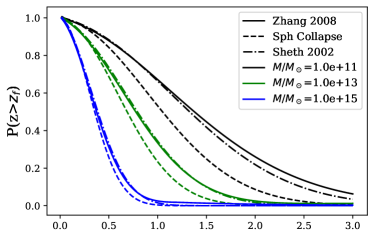
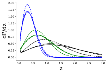
Figure 3: Cumulative (top panel) and differential (bottom panel) distributions of the formation redshift $z_{50}$ in our fiducial cosmology, for the SC model (Lacey & Cole, 1993, dashed lines), and the EC models from Sheth & Tormen (2002, dot-dashed lines) and Zhang et al. (2008, solid lines).

2.4 Cosmological Dependence of Halo Assembly Time

Given a prediction for the distribution of halo formation redshifts, we can study how it varies with cosmological parameters. We have tested the dependence of three quantities in particular:

• The median formation redshift, defined as $\left<z_{50}\right>=z_{m}$ such that $P(Z>z_{m})=0.5$

• The peak of the differential probability distribution, $z_{p}=\rm{max}\left[\frac{dP}{dz}(z)\right]$

• The average formation redshift, $z_{a}=\int_{z_{obs}}^{\infty}z\,\frac{dP}{dz}dz$ .

Of these three, we will focus on the median formation redshift, noting that the average formation redshift is slightly higher.

Both spherical and ellipsoidal collapse models predict the same behaviour of the median formation time, as shown in Fig. 4. Haloes form earlier in high–$\sigma_{8}$ cosmologies, since a greater mean fluctuation amplitude causes typical peaks in the density field to cross the threshold for collapse earlier in the process of structure formation. The $\Omega_{\rm m}$-dependence is less trivial and differs between low-mass and high-mass haloes. As explained in Appendix C, high-$\Omega_{\rm m}$ cosmologies have more power on small scales relative to large ones. Thus at fixed $\sigma_{8}$, low-mass haloes form earlier in higher $\Omega_{\rm m}$ universes, while high mass haloes form slightly later. This agrees with the previous findings of Giocoli et al. (2012).

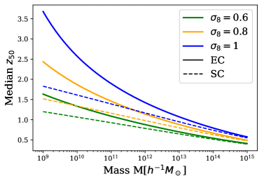
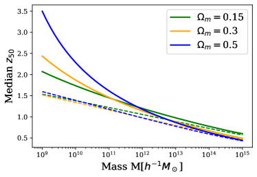
Figure 4: Mass dependence of the median formation redshift $\left<z_{50}\right>$, for haloes at $z=0.15$, and for different values of $\sigma_{8}$ (left panel) and $\Omega_{\rm m}$ (right panel). Solid lines show the ellipsoidal collapse predictions; dashed lines show the spherical collapse predictions.

The general dependence of formation epoch $z_{50}$ on $\Omega_{\rm m}$ and $\sigma_{8}$ is shown in Fig. 5. The main trend is for age to increase with $\sigma_{8}$; since the masses shown here are all beyond the cross-over point in Fig. 4, median age also decreases slightly with $\Omega_{\rm m}$, particularly at large masses. We explore how the dependence of $z_{50}$ on $\Omega_{\rm m}$ and $\sigma_{8}$ arises in more detail in Appendix D.

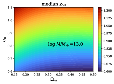
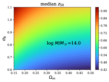
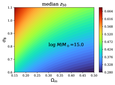
Figure 5: Median $z_{50}$ for present-day haloes of the mass indicated, as a function of $\Omega_{\rm m}$ and $\sigma_{8}$. Calculations assume the EC model (cf. Sec.2.3).

Comparing Figs. 2 and 5 closely, we note an important feature of halo age relative to halo abundance: for lower mass haloes and/or at lower redshift, the contours for the two are fairly orthogonal over much of the $\Omega_{\rm m}$–$\sigma_{8}$ plane. To highlight this point, Fig. 6 shows the two sets of contours superimposed, for the ranges of mass and redshift accessible to large cluster surveys. In the region of particular interest, around the concordance model ($\Omega_{\rm m}=0.3$, $\sigma_{8}=0.8$), the two sets of contours are almost exactly orthogonal for lower masses and/or redshifts, where $\nu\sim$2–3 (top and middle left hand panels). They only become similar for the most massive clusters, at $z\geq 1$, where $\nu\sim 4$–6 (bottom right panel). This implies that age or age proxies, measured for clusters with masses $M<5\times 10^{14}M_{\odot}$ at $z<1$, can potentially break the main degeneracy in cluster abundance measurements.

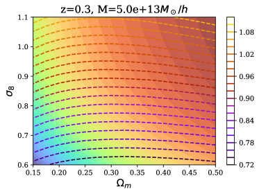
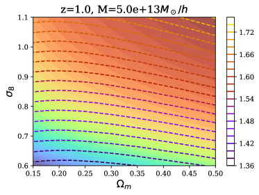
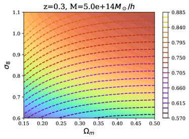
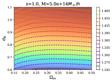
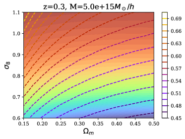
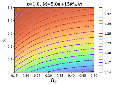
Figure 6: A comparison of age and abundance contours in the $\Omega_{\rm m}$–$\sigma_{8}$ plane, for the halo mass and redshift indicated at the top of each panel. Filled contours show curves of constant number density per unit log $M$. Dashed lines show curves of constant $z_{50}$, with the scale given by the colorbar.

3 Comparison to simulations

3.1 Simulation Data

In Section 2.3, we provided analytic EPS estimates of how the halo formation time $z_{50}$ depends on $\Omega_{\rm m}$ and $\sigma_{8}$. Given the approximations made in these models, it is worth testing the accuracy of their predictions in N-body simulations.

Previous work has demonstrated that different merger tree algorithms can produce significantly different MAHs (Avila et al., 2014; Srisawat et al., 2013). The exact value of $z_{50}$ may be particularly sensitive to these differences, as discussed in Srisawat et al. (2013). In particular, some merger tree algorithms allow fragmentation events, where haloes lose mass with time, such that MAHs are not always monotonic. Our previous EPS estimates assume strictly hierarchical growth, and thus we anticipate that the numerical results may disagree with them to some degree. To test the effect of different methods of analysis, we consider three sets of simulations (two public, and one of our own), that employed three different merger tree algorithms:

• The Illustris TNG simulation, (Nelson et al., 2019) using the Sublink merger tree algorithm (Rodriguez-Gomez et al., 2015).

• The Bolshoi/BolshoiP simulation, (Klypin et al., 2011) using the Rockstar halo finder (Behroozi et al., 2013a) and the Consistent Trees merger tree code (Behroozi et al., 2013b). (Note that Bolshoi uses WMAP cosmological parameters, whereas BolshoiP uses Planck ones.)

• Our own set of 9 cosmological simulations, spanning a range of cosmological parameters, and analyzed using the AHF halo finder and merger tree code (Knollmann & Knebe, 2009; Gill et al., 2004). These will be labelled MxSy, where $x=25/3/35$ indicates the value of $\Omega_{\rm m}$, and $y=7/8/9$ indicates the value of $\sigma_{8}$.

The simulation parameters are summarized in Table 1. Data from the TNG and Bolshoi simulations were obtained directly from their respective websites. In particular, we used the Rockstar merger tree data available for the Bolshoi simulation. For the TNG and MxSy simulations, mass accretion histories were calculated using the Sublink and AHF codes, respectively. For the Bolshoi simulations, they were generated by following the main progenitor sequence in the Rockstar files.

Simulation	$\Omega_{\rm m}$	$\sigma_{8}$	particle mass [$M_{\odot}/h$]	$N_{\rm part}$	merger tree	$N_{\rm snap}$
Illustris TNG	0.31	0.81	$3\times 10^{9}$	$625^{3}$	Sublink	100
Bolshoi	0.27	0.82	$1.35\times 10^{8}$	$2048^{3}$	Consistent Trees	181
BolshoiP	0.31	0.82	$1.55\times 10^{8}$	$2048^{3}$	Consistent Trees	178
MxSy	0.25/0.3/0.35	0.7/0.8/0.9	$4\times 10^{9}$	$512^{3}$	Amiga Halo Finder	44

Table 1: Summary of the simulations used and their main parameters, including cosmological parameters, particle mass, total number of particles $N_{\rm part}$, merger tree code, and the number of snapshots $N_{\rm snap}$ used to make the merger trees. The MxSy simulations are a set of 9 of our own simulations that span a range of different values of $\Omega_{\rm m}$ and $\sigma_{8}$.

3.2 Formation Time Distributions Compared

In each numerical MAH, we define $z_{50}$ to be the lowest redshift at which the mass of the halo has dropped to less than half of the mass at $z=0$. Fig. 7 compares the distribution of these formation redshifts to the analytic (EC) predictions. For all three simulations considered, but particularly for the Bolshoi and M3S8 simulations, we see a clear offset between the numerical results and the EC predictions, that is largest at small masses. In general, the numerical formation redshifts are larger than predicted, by up to 0.1–0.2 on average.

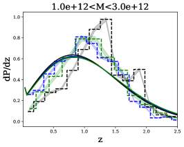
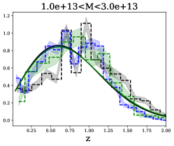
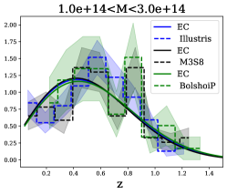
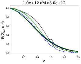
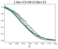
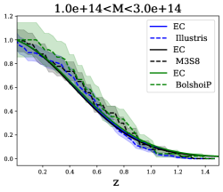
Figure 7: Differential (top) and cumulative (bottom) distributions of $z_{50}$ in our fiducial cosmology, for three different ranges of halo mass. Smooth curves show the (EC) analytic prediction, while dashed lines with shading show the numerical results and associated Poisson uncertainties.

One possible explanation for this shift lies in the different definitions of merger time assumed. Given a particular merger event, EPS theory takes the corresponding collapse redshift (that is, roughly, the time by which newly-accreted mass has first fallen to the centre of the halo) to be the moment at which a halo’s virial mass is said to increase. In contrast, numerical group finders may link haloes when their outer virial surfaces first touch. Thus, numerical mergers may occur up to one infall time earlier than analytic ones. Adding a delay equal to the infall time to the numerical results, we obtain the $z_{50}$ distributions in Fig. 8. The discrepancy between the numerical and analytic results is greatly reduced, although some differences remain, as seen most clearly in the cumulative distributions.

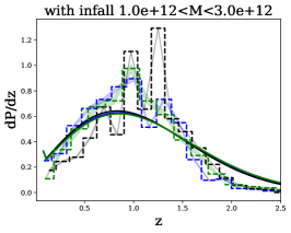
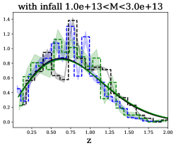
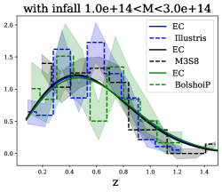
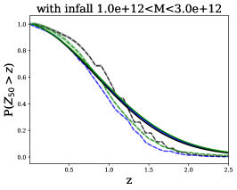
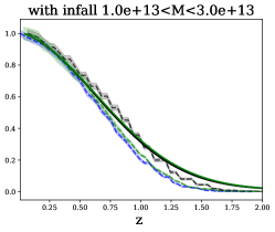
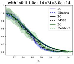
Figure 8: Differential and cumulative $z_{50}$ distributions, as in Fig. 7, after taking into account the delay due to infall.

The remaining differences may have several possible explanations. There are slight offsets between the distributions for the three simulations, suggesting that the different halo finders and merger tree algorithms used to analyze them affect the results. A detailed comparison of halo finders and merger tree algorithms, including AHF, Rockstar/ConsistentTrees and Subfind/Sublink, was presented in Knebe et al. (2011). They highlight a number of significant differences between methods, notably in how they treat fragmentation events and non-monotonic MAHs. We note that the discrepancy between numerical and analytic results is greatest at low mass, so resolution may also play a role. Finally, even the revised EC version of EPS remains an approximate theory, so its predictions may be inaccurate at some level.

We summarize the comparison between numerical and analytic results in Fig. 9, which shows the median $z_{50}$ of each of the simulations, together with the uncertainty (points with errorbars), compared to the analytical predictions from the EC model of Zhang et al. (2008). As discussed in Section 2.4, age is most sensitive to the amplitude of fluctuations $\sigma_{8}$, and depends only weakly on $\Omega_{\rm m}$. At high mass, the numerical results agree well with the analytic prediction, at least in terms of the median value of $z_{50}$. Since this mass range is the one relevant for cluster surveys, we conclude that our previous analytic estimates are reasonably valid, although the details of the halo age distribution require further study in future work.

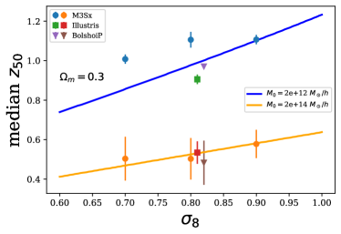
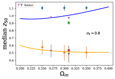
Figure 9: Median value of $z_{50}$ for present-day haloes, as a function of $\sigma_{8}$ (left panel) and $\Omega_{\rm m}$ (right panel). Smooth curves show the EC prediction; points with error bars show the numerical results and Poisson uncertainties, corrected for infall time. Each symbol represents a different set of simulations and different point colors represent different masses. Note that on the right panel two versions of Bolshoi are shown, one with Planck cosmology and one with WMAP cosmology. See Table 1.

4 Observational prospects

A number of ongoing and future surveys are expected to produce very large samples of galaxy clusters, with $O(10^{5})$ significant detections, out to redshifts of $z=1$ or higher (e.g. Pillepich et al., 2012; Sartoris et al., 2016; Abazajian et al., 2019). Supposing such a sample were available, with age information based on one or more observational proxies, we can ask what sensitivity this dataset would have to the cosmological parameters, or equivalently how large a sample would be needed to provide significant improvement on parameter constraints.

To estimate age observationally, we need a structural proxy for age (as expressed, say, by the formation epoch $z_{50}$). There are several known examples of structural properties that correlate with $z_{50}$ Wong & Taylor (2012), including concentration (Zhao et al., 2003; Wang et al., 2020), shape (as a product of major mergers -Drakos et al. 2019a), substructure (e.g. Gao et al., 2004; Taylor & Babul, 2005; Diemand et al., 2007), or overall degree of relaxation, as measured by a centre-of-mass offset (Macciò et al., 2007; Power et al., 2012). We will take concentration as an example here, as its age dependence is the best studied. We note that on some mass scales and at some redshifts, baryons may have an important effect on halo structure, and on concentration specifically. We will start by discussing concentration measurements ignoring these possible effects, but then consider them separately in Section 4.4 below.

4.1 Mean Concentration versus $z_{50}$

Since the discovery of the universal density profile (Navarro et al., 1997, NFW hereafter), the value of the concentration parameter $c=r_{\rm vir}/r_{\rm s}$ has been linked to the halo’s formation history. In NFW, concentration depends on how early a critical fraction of the final mass was first assembled into (any number of) progenitors. Subsequent models (e.g. Bullock et al., 2001; Wechsler et al., 2002; Zhao et al., 2003, 2009; Ludlow et al., 2014; Correa et al., 2015a) related concentration instead to the growth history of a single main progenitor, as expressed by the mass accretion history (MAH). In the simplest picture (Wechsler et al., 2002; Zhao et al., 2003), $c\simeq$ $c_{0}(a_{0}/a_{r})$ where $a_{r}$ is the scale factor at the end of the period of rapid growth in the MAH, and $c_{0}\sim 3$–4 is the concentration of newly-formed systems at this time. In these models, there is, therefore, a direct correlation between $c$ and $z_{50}$, or any similar estimate of the formation epoch $z_{\rm f}$ (Wong & Taylor, 2012).

All of these models focus on the relation between the average growth rate and the mean concentration of a sample of haloes of a given range of mass and redshift (although Ludlow et al. 2013 does consider the connection between individual MAHs and concentration values.) Major mergers can lead to large variations in concentration, however, depending on the net input of (orbital) energy (Drakos et al., 2019b). Most recently, Wang et al. (2020) have shown that the measured value of the concentration parameter oscillates during major mergers, and that these fluctuations may dominate the statistics of the average values measured for large ensembles. Clearly, the subject is complicated and requires further study; we will not consider it in further detail here, but will assume a correlation between $c$ and $z_{50}$, that makes mean concentration measurements sensitive to mean age.

Fig. 10 shows this correlation in practice, as measured from our grid of MxSy simulations for different cosmological parameters (we have chosen a lower halo mass range, 1–3$\times 10^{12}M_{\odot}$, to reduce Poisson noise in the figure). The basic pattern is similar for each set of cosmological parameters, and has been explored extensively in the literature (e.g. Wechsler et al., 2002; Zhao et al., 2003, 2009; Giocoli et al., 2012; Correa et al., 2015b; Ludlow et al., 2013), though interestingly, there is also a slight change in the mean relation over the range of parameters explored. In particular, the intercept of the linear regression relation between $\log c$ and $\log(1+z)$ increases monotonically, both with $\Omega_{m}$, and with $\sigma_{8}$. This indicates that the concentration has an additional cosmological sensitivity, beyond its main dependence on formation history. Here too, there is clearly further complexity to explore in the concentration-mass-redshift relation; in future work, we will focus on understanding and calibrating the mean $c(z,M)$ and $c$–$z_{50}$ relationships, and consider more generally the links between concentration, mass accretion history, and cosmology. For the purpose of our present calculations, we will assume a power-law correlation with a fiducial scatter of 30%, which provides a reasonable fit to the results from all nine cosmologies.

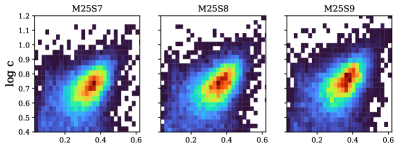
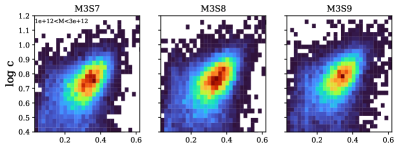
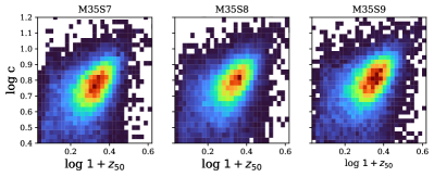
Figure 10: Concentration versus $z_{50}$ for present-day haloes with masses between $10^{12}M_{\odot}$ and $3\times 10^{12}M_{\odot}$, in the 9 MxSy simulations.

4.2 Measured Concentration versus Mean Concentration

From the preceding results, the actual 3D concentration of an individual halo should scatter by $\sim 30$% for a given value of $z_{50}$. This actual concentration can be estimated in various ways, including weak lensing convergence, detailed modelling of the lensing potential in strong lensing systems, X-ray or SZ emission, or even the galaxy distribution within a group or cluster. Each of these techniques will add observational errors and biases; see, for instance, Groener et al. (2016), which provides a fairly recent review of individual concentration estimates in clusters. Generally, the observational errors are 0.1 or 0.2 dex, i.e. 25–60%, for each individual system. There are also systematic uncertainties, both identified and unidentified, associated with each method. In principle, future work with large samples, dedicated simulations, and comparison between observational modalities may help reduce these. Overall, we will assume typical errors of either 30% or 50% in going from an actual 3D concentration to an observational estimate.

Combining these errors with the intrinsic scatter in the $c$–$z_{50}$ relation, we expect a net scatter of $\epsilon_{z_{50}}=$ 40–60% in the relation between an observational estimate of concentration and the formation epoch $z_{50}$. This large uncertainty makes individual measurements relatively uninteresting; we can compare the situation to weak gravitational lensing, however, where shape measurements for individual galaxies are extremely noisy, but careful averaging extracts the mean value in an unbiased way.

4.3 $z_{50}$ versus Cosmology

The remaining factor in our calculation is the connection between an estimate of the mean value of $z_{50}$ and the values of the cosmological parameters. From Fig. 9, to achieve a nominal precision of 0.01 in $\sigma_{8}$, we need 0.55% precision in the estimate of $\langle z_{50}\rangle$. Assuming unbiased averaging over a sample of $N$ clusters, $\sigma\langle z_{50}\rangle=\epsilon_{z}/\sqrt{N}$. Solving, we get $N=(0.40/0.0055)^{2}$–$(0.60/0.0055)^{2}\sim$ 5,000–12,000. Thus, with low-precision but unbiased concentration measurements for $O$(10,000) clusters, we could obtain constraints on the value of $\sigma_{8}$ that correspond to 1/10 or less of the current range of uncertainty in this parameter.

4.4 Baryonic Corrections

A major uncertainty in the preceding calculations is the net effect of baryons on cluster concentrations. Baryons may alter the halo density profile, increasing halo concentration via adiabatic contraction, or reducing it through outflows driven by stellar or AGN feedback. These effects are complex, and depend on mass, redshift, and radius within the halo. Overall, these processes can affect halo concentration and masses significantly (Debackere et al., 2021). Although simulations suggest that baryonic effects are largest in galaxy-scale haloes (e.g. Velliscig et al., 2014), they may still be significant when measuring concentration or internal structure in clusters – Debackere et al. (2021), for instance, find a 10% bias in estimates of the scale length $r_{s}$ at masses of 5$\times 10^{14}h^{-1}M_{\odot}$.

Baryonic effects are not yet well enough understood to include in our predictions; in particular, their detailed dependence on the cosmological parameters is not yet known. We can point out a few possible avenues, however, to calibrating and correcting for their effects on structural measurements. First, simulations now model these effects with increasing accuracy, allowing the potential for calibration of any net bias in structural properties. Second, observations of nearby, well-studied systems allow verification of the simulations, independent of the samples used for cosmological tests. Third, as pointed out in Section 2.4, over some mass and redshift ranges, cluster age and abundance are predicted to vary almost identically with the cosmological parameters $\Omega_{\rm m}$ and $\sigma_{8}$. This should provide an independent test of any assumed concentration-mass relationships, at least for this range of mass and redshift, as the constraint in the $\Omega_{\rm m}$–$\sigma_{8}$ plane derived from age/concentration measurements must agree with the one derived from abundance, and since the contours for the two are parallel, there is little room for bias in one relative to the other.

A final, and basic, reason for optimism is the differential nature of structural tests, whether based on concentration or on other structural properties. These would depend on the relative distribution of structural properties, measured across a population of systems. A simple proxy for the mean age of the sample, for instance, might be the number of high-concentration systems, relative to low-concentration ones. Thus, to lowest order, a net shift in concentration for the whole population would largely cancel out, reducing the bias in the final results. At the same time, the shape of the measured concentration distribution for the whole sample would provide another test of the consistency of the method, and any biases or effects due to sample selection.

Overall, it is clear that the impact of baryonic effects on halo structure requires much more detailed study, to see whether and to what degree they would compromise structural tests of cosmology, for a given survey and methodology.

4.5 What is Achievable?

In summary, in previous sections, we have shown that with low-precision but unbiased concentration estimates for $O(10^{4})$ clusters, one could obtain excellent constraints on $\sigma_{8}$, assuming the net effect of baryons is small, or can be corrected using simulations. While measuring concentration observationally is challenging, our method does not require particularly accurate measurements for individual systems – given the intrinsic scatter in the $c$–$z_{50}$ relation, the errors in individual estimates need only be accurate at the $\sim$30% level.

We can consider this goal in more detail for a particular survey. The Euclid mission is a 1.2m space telescope, operating in the visible and near-infrared (NIR). As part of its wide survey, it will image 15,000 deg² of the sky in one optical and three NIR bands, detecting galaxies down to an AB magnitude of 24 or fainter. Photo-zs will be derived for these objects, using ancillary data from ground-based surveys such as UNIONS (Chambers et al., 2020). The Euclid wide survey should provide large catalogues of clusters detected photometrically (that is by clustering in projection and in photo-z space), and also as peaks in weak lensing maps. Based on the forecasts of (Sartoris et al., 2016), the photometric detections should include all clusters with masses $M\gtrsim 10^{14}M_{\odot}$ out to redshift $z\sim 2$. Below redshift z = 0.5, the wide survey is expected to detect 1.5 million clusters at 3$\sigma$ or greater significance, and 200,000 clusters at 5$\sigma$ significance. Extrapolating from these predictions, the number of 7$\sigma$ detections is in excess of 20,000 (with half that number at redshifts $z<0.7$). Admittedly, these objects may be slightly more massive than the example considered above in section 4.3 ($3.5\times 10^{14}M_{\odot}/h$, versus $2\times 10^{14}M_{\odot}/h$) but they are close enough that the slope of the $\langle z_{50}\rangle$–$\sigma_{8}$ relation should be similar.

The Roman Space Telescope mission is a 2.4m wide-field space telescope, with optical/NIR imaging and slitless spectroscopy capabilities. Its High Latitude Survey will image $\sim$2000 deg² of sky in four NIR bands, reaching depths 1–2 AB magnitudes deeper than Euclid Wide, as well as providing slitless spectroscopy of brighter targets. This deeper data over a smaller area should produce a cluster sample that extends to lower masses and higher redshifts, and thus provides an interesting counterpoint to Euclid data. In particular, we note that at high redshift, the complementarity of age and abundance is reduced (cf. the left-hand panels of Fig. 6). This could provide an important consistency check on age estimates, as discussed previously. Finally, a number of other forthcoming experiments expect to detect large numbers of clusters, including eROSITA (Pillepich et al., 2012) in the X-ray, CMB-S4 (Abazajian et al., 2019) in the mm, and the ground-based UNIONS (Chambers et al., 2020), DESI (DESI Collaboration et al., 2016), and Rubin LSST (LSST Science Collaboration et al., 2009) surveys.

Overall, we conclude that multiple samples of $O(10^{4})$ clusters with sufficient signal-to-noise ratio (SNR) to allow structural measurements should become available in the near future. One could imagine using a large, uniform survey such as Euclid for the low-redshift sample selection, together with other complementary observations to make structural measurements on individual clusters. A high-redshift sample could then be used to test and calibrate age proxies, as mentioned above. It might also be possible to stack clusters to use a mean projected density profile, measured at high SNR, to derive constraints. We will consider these and other approaches in future work.

As in weak lensing studies, the challenge of averaging over large numbers of low SNR measurements will be in controlling for and reducing systematics. Beyond the baryonic effects discussed in the previous section, systematics related to basic structure formation could also affect sample selection (e.g. by preferentially highlighting or neglecting disturbed systems); they could bias individual mass estimates (although the slope of the concentration-mass relation is fairly shallow, so accurate masses are less important than in abundance studies); or they could bias concentration measurements, e.g. by biasing the sample selection towards objects with a particular 3D shape, or with a disturbed IGM (if the confirmation or structural measurements are performed in the X-ray). In lensing-based studies, false peaks and projections could be a particular problem, as these may look less regular and have lower concentrations, biasing the average. Environment can also have an impact on formation time through assembly bias, as simulations have shown that haloes form earlier in dense environments (Gao et al., 2005; Wechsler et al., 2006; Harker et al., 2006), so unbiased sampling of large volumes is important. Here again, there is much future work to be done considering the the possible biases for different observational modalities and survey strategies.

5 Conclusion

The enormous success of CMB analyses and large cosmological surveys over the last few decades has been driven, for the most part, by a robust and detailed understanding of structure formation in the linear regime. Cluster number counts are an important exception, but they only probe one limited aspect of non-linear structure formation. As cluster catalogues grow by several orders of magnitude in size over the next decade, it is worth considering what other cosmological information we might extract from them. Measurements of internal halo structure can, in principle, tell us about the rate of non-linear structure formation, and are worth considering as a next-generation cosmological test.

Previous work has established that as haloes grow through hierarchical merging, this process leaves structural signatures that can last for many dynamical times, that is, for many Gyr at low redshift. As a result, structural measurements provide several different avenues to estimate cluster assembly times or “ages”. In this paper, we have shown that for typical clusters at $z<1$, age varies almost orthogonally to abundance in the space of the cosmological parameters $\Omega_{\rm m}$ and $\sigma_{8}$. The same datasets that provide abundance constraints could be used to estimate mean values for structural parameters, and thus age, providing significantly tighter parameter constraints from a single set of observations.

Of course, given the accuracy of current constraints from the CMB, it may seem less interesting to invest further in other techniques. A survey of current results hints at tension between the different measurements, however, emphasizing the importance of redundant cosmological tests, over different ranges of redshift, mass and/or spatial scale. To resolve the deep mysteries of dark energy and dark matter, and to rule out yet-undiscovered variations on the current cosmological model, we need to test it as sensitively as possible, across as broad as possible a range of parameter space. In pursuit of this goal, our growing understanding of non-linear structure formation will open up many exciting possibilities for new tests and new tools.

Data Availability

N-body simulation data from the Bolshoi simulation is publicly available (after registration) at https://www.cosmosim.org/. N-body simulation data from the Illustris TNG simulation is publicly available (after registration) at https://www.tng-project.org/. The rest of the data underlying this article will be shared on reasonable request to the corresponding author.

Appendix A Details of the Analytic Calculations

We use standard tools and techniques for the analytic calculations in Section 2. In particular, the growth factor $g(z)$ is calculated using the approximation given by Carroll et al. (1992), which is accurate to a few percent:

$$g(z)\approx\frac{5\Omega_{m}(z)}{2\left[\Omega_{m}^{4/7}(z)-\Omega_{\Lambda}(z)+(1+\Omega_{m}(z)/2)(1+\Omega_{\Lambda}(z)/70)\right]}\,.$$ (14)

The critical overdensity $\delta_{c}$ is the value a linearly-extrapolated density perturbation needs to reach to collapse and form a virialized object, and can be estimated using the spherical collapse model. Its present-day value varies weakly with $\Omega_{m}$ (Mo et al., 2010):

$$\delta_{c}=\frac{3}{5}\left(\frac{3\pi}{2}\right)^{2/3}\Omega_{m}^{0.0055}\approx 1.686\Omega_{m}^{0.0055}\,.$$ (15)

The linear matter power spectrum

$$P(k)=Ak^{n_{s}}T(k)$$ (16)

is computed using the approximation to the transfer function $T(k)$ given by Equation 16 in Eisenstein & Hu (1998). We take the primordial amplitude to be A=1 initially, and then adjust this value retroactively to set the correct value for $\sigma_{8}$. The index of the primordial spectrum is taken to be $n_{s}=0.965$.

The variance of the density fluctuation field, $\sigma^{2}$, is computed numerically by convolving the power spectrum $P(k)$ with a top hat smoothing filter:

$$\sigma^{2}(R)=\frac{1}{2\pi^{2}}\int_{0}^{\infty}k^{2}P(k)\widetilde{W}_{R}^{2}(k)dk\,,$$ (17)

where

$$\widetilde{W}_{R}(k)=3\frac{\sin(kR)-kR\cos(kR)}{(kR)^{3}}$$ (18)

We have compared our derived values of $P(k)$ and $\sigma(M)$ to values calculated using the Colossus python package (Diemer, 2018), and find good agreement.

Appendix B Survey mass versus $\Omega_{\rm m}$

Halo abundance depends on the total mass of material sampled in a survey volume, $M_{V}$, and on the collapsed fraction $f$ at that scale and redshift. The survey mass obviously depends on the mean matter density $\rho_{m}$ and thus on $\Omega_{m}$ directly, but it also depends on $\Omega_{m}$ indirectly, through the volume sampled for a given solid angle and redshift range. The left panel of Fig. 11 shows the total mass contained within a survey volume per unit redshift per unit solid angle at two different redshifts, as a function of the cosmological parameter $\Omega_{\rm m}$. While the volume element is a decreasing function of $\Omega_{\rm m}$ for flat $\Lambda$CDM cosmologies (since volume at a given redshift grows as $\Lambda$ increases), the total mass enclosed increases overall, with the greatest $\Omega_{\rm m}$ sensitivity at low redshift.

In the end, however, the total mass $M_{V}$ has relatively little influence on the overall shape of the abundance contours in the $\Omega_{m}$–$\sigma_{8}$ plane, because its variation is of order a factor 2 or less, while the collapsed fraction varies over several orders of magnitude as $\Omega_{m}$ changes (right panel of Fig. 11; see Appendix C for a discussion of the parametric dependence of the collapsed fraction).

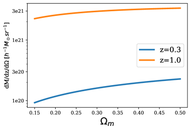
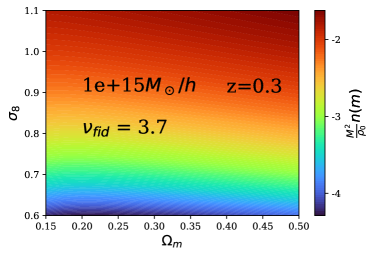
Figure 11: Left : total mass $M_{V}$ contained within a survey volume, per unit solid angle and per unit redshift interval, as a function of $\Omega_{\rm m}$, at redshifts 0.3 and 1 (note a flat $\Lambda$CDM cosmology is assumed). Right : Variation of the (EC) collapsed fraction $f_{\rm ST}$ in the $\Omega_{\rm m}$–$\sigma_{8}$ plane, for the particular choice of halo mass and redshift indicated. Note the similarity to the dependence of peak height (Fig. 1), although the colour scale here is now inverted, and logarithmic.

Appendix C Peak Height and collapsed fraction versus $\Omega_{\rm m}$ and $\sigma_{\rm 8}$

We can write peak height as the product of three factors:

$$\nu=\frac{\delta_{c}(z)}{\sigma(M)}=\frac{\delta_{c}(z)}{\sigma_{8}\Gamma(M)}\,,$$ (19)

where we have defined $\Gamma(M)\equiv\sigma(M)/\sigma_{8}$. The redshift evolution of the collapse threshold stems from the linear growth of fluctuations

$$\delta_{c}(z)=\delta_{c}(0)\frac{D(0)}{D(z)}=\delta_{c}(0)\frac{a_{0}g(0)}{ag(z)}\,,$$ (20)

where $D$ is the fluctuation amplitude, $g$ is the linear growth factor, and $a$ is the scale factor. Combining these,

$$\nu=\frac{(1+z)}{\sigma_{8}}\frac{1}{\Gamma(M)}\frac{\delta_{c}(0)}{g(z)/g(0)}\,.$$ (21)

Thus, while peak height scales simply as $1/\sigma_{8}$, the dependence on $\Omega_{\rm m}$ is through both the shape of the matter power spectrum $\Gamma(M)$ and the relative growth factor $g(z)/g(0)$. We consider each of these in turn.

C.0.1 $\Gamma(M)$

The function $\Gamma(M)$ describes the shape of the amplitude of fluctuations as a function of mass, $\sigma(M)$, independent of its normalization $\sigma_{8}$. This shape will depend on the value of the matter density parameter $\Omega_{\rm m}$. More specifically, in cosmologies with larger matter densities, matter-radiation equality occurs sooner. Growth is suppressed by radiation on all scales below the horizon scale at recombination, but these scales are smaller and spend less time inside the horizon when $\Omega_{\rm m}$ is larger. Thus, for a fixed amplitude $A$ of the primordial power spectrum, small-scale power at recombination will increase with $\Omega_{\rm m}$ (dashed curves in the top left panel of Fig. 12).

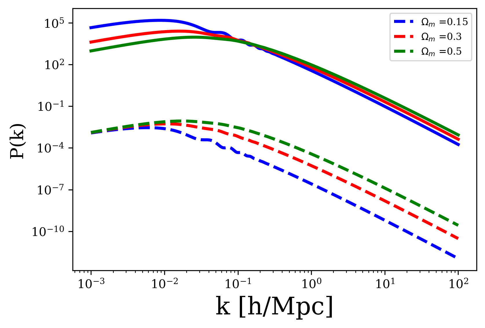
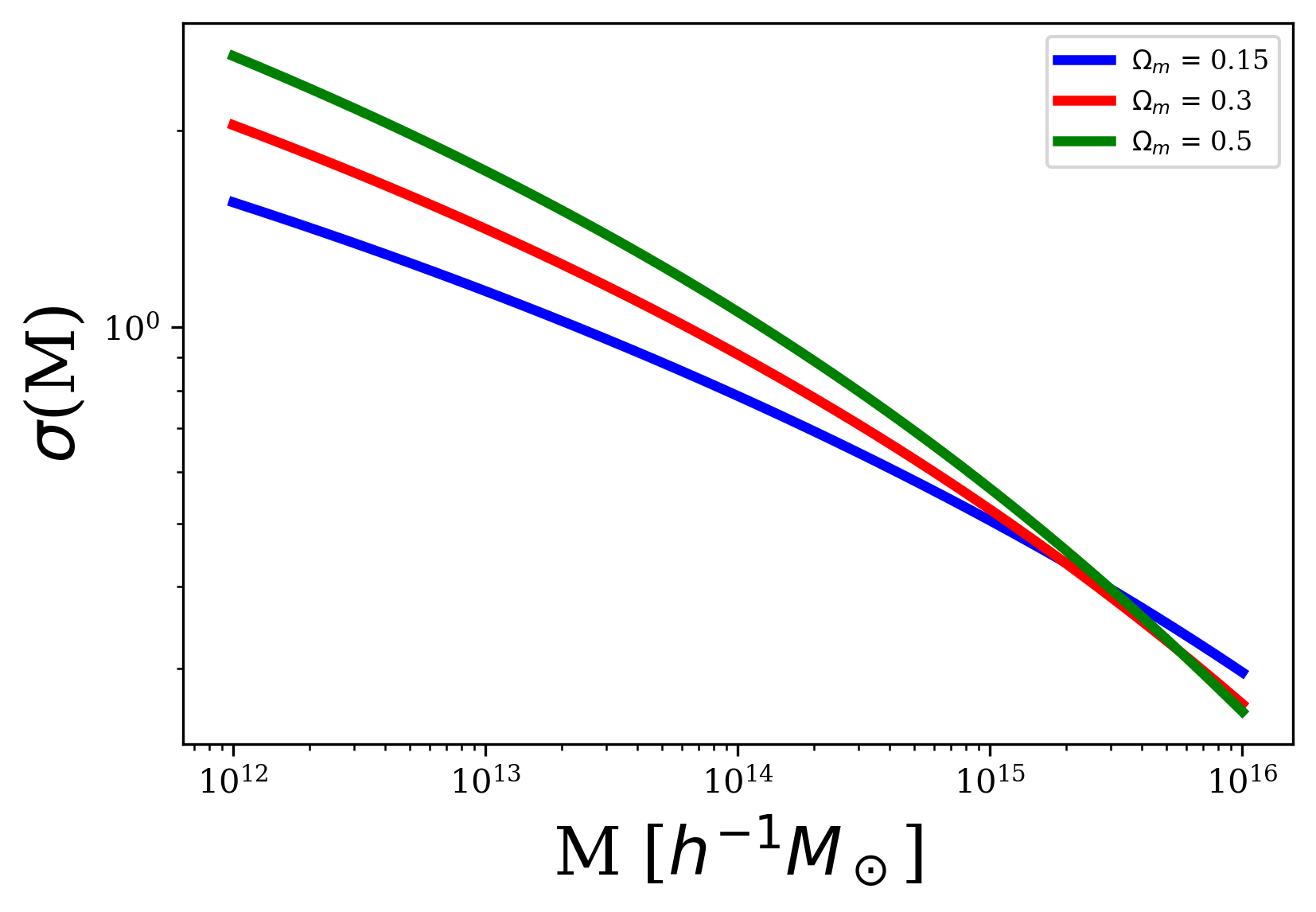
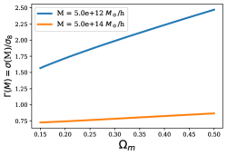
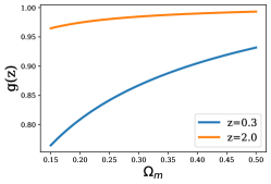
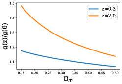
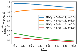
Figure 12: Upper left: Variation of the power-spectrum $P(k)$ with $\Omega_{\rm m}$ at fixed primordial amplitude (dashed lines) and for fixed $\sigma_{8}$ (solid lines). The upper middle and upper right panels show how $\sigma(M)$ and $\Gamma(M)$ depend on $\Omega_{\rm m}$. The lower left and lower middle panels show how the growth factor and the normalized growth factor vary with $\Omega_{\rm m}$. The lower right panel shows how, as a consequence of these dependencies, the peak height $\nu$ varies with $\Omega_{\rm m}$ at fixed $\sigma_{8}$, following Eq. 25.

Fixing $\sigma_{8}$, the amplitude of fluctuations at scales of $8h^{-1}$Mpc, reduces some of the difference in power (solid curves in the top left panel of Fig. 12), but the shape of $\sigma(M)$ remains steeper in cosmologies with larger values of $\Omega_{\rm m}$ (top middle panel of Fig. 12). Thus, over the range of interest, the ratio $\Gamma=\sigma(M)/\sigma_{8}$ increases with $\Omega_{\rm m}$, especially at lower mass (top left panel of Fig. 12). We can model this dependence as

$$\Gamma(M)\sim\Omega_{\rm m}^{\beta(M)}\,,$$ (22)

where $\beta(M)$ decreases with mass, and becomes negative at $M=M_{8}\approx 2\times 10^{15}M_{\odot}/h$ where $\sigma(M)=\sigma_{8}$.

C.0.2 Growth factor

The lower panels of Fig. 12 show how $g(z)$ and $g(z)/g(0)$ vary with $\Omega_{\rm m}$. In a flat $\Lambda$CDM model, the growth factor $g(z)$ at a fixed redshift $z$ is reduced for low $\Omega_{\rm m}$, as dark energy suppresses the growth of fluctuations. The relative amplitude of the effect is greater for very low values of $\Omega_{\rm m}$, or for large redshift ranges, and thus the ratio $g(z)/g(0)$ is largest for low $\Omega_{\rm m}$ and/or high redshift (middle panel). Mathematically, we can estimate the dependence on the density parameter by using the approximation $g(z)\propto\Omega_{\rm m}^{3/7}(z)$ (Carroll et al., 1992):

$$\frac{g(z)}{g(0)}\propto\left(\frac{\Omega(z)}{\Omega_{0}}\right)^{3/7}\propto\left(\frac{{\bar{\rho}_{m}}(z)\rho_{c}(0)}{{\bar{\rho}_{0}}\rho_{c}(z)}\right)^{3/7}\propto\frac{((1+z)^{3})^{3/7}}{E(z)^{3/7}}\propto\Omega_{\rm m}^{-\alpha(z)}\,,$$ (23)

where

$$E(z)=\frac{H(z)}{H(0)}\sim\sqrt{(1+z)^{3}\Omega_{\rm m}+\Omega_{\Lambda}}$$ (24)

is the Hubble ratio. The index $0<\alpha(z)<1$ is an increasing function of $z$, and approaches the value $3/14$ at high redshift.

C.0.3 Peak Height

Given these results, the overall dependence of the peak height on $\Omega_{\rm m}$ and $\sigma_{8}$ can be written

$$\nu(M,z)\propto\frac{1}{\sigma_{8}}\Omega_{\rm m}^{\alpha(z)}\Omega_{\rm m}^{-\beta(M)}\,,$$ (25)

where $\alpha>0$ and increases with redshift to the limiting value $3/14$, while $\beta(M)$ is a decreasing function of mass, and is negative at large masses. Combining the positive slope of $\Gamma$ with the negative slope of $g(z)/g(0)$, the bottom right-hand panel of Fig. 12 shows how $\nu$ generally decreases with $\Omega_{\rm m}$, but can increase for large masses and high redshifts. This explains the slight $\nu$-dependence seen in Fig. 1. The summary of how the peak height varies with mass and redshift for different values of $\Omega_{m}$ and $\sigma_{8}$ is shown in Fig. 13.

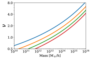
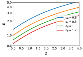
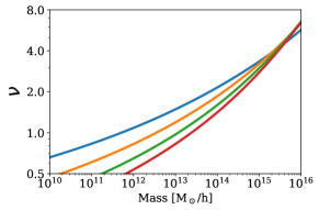
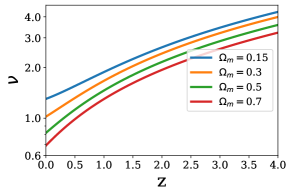
Figure 13: Variation of the peak height $\nu$ with mass (left panels) and redshift (right panels), for different values of the cosmological parameters. The two top panels show the dependence on $\sigma_{8}$ at fixed $\Omega_{\rm m}=0.3$, while the bottom panels show the dependence on $\Omega_{\rm m}$ at fixed $\sigma_{8}=0.8$.

C.0.4 Collapsed Fraction

Combining the peak height dependence described above with the functional form of the collapsed fraction as a function of peak height (Eqs. 3 or 4) we obtain the collapsed fraction as a function of mass for different values of $\sigma_{8}$ and $\Omega_{m}$, shown in the left and right panels of Fig. 14 respectively. It shows two regimes, a power-law increase at low masses, followed by an exponential decrease for cluster mass haloes. The figure also shows why the collapsed fraction sensitivity to $\sigma_{8}$ and $\Omega_{m}$ varies with mass, and the transition between the two regimes occurs at different masses for different values of $\sigma_{8}$.

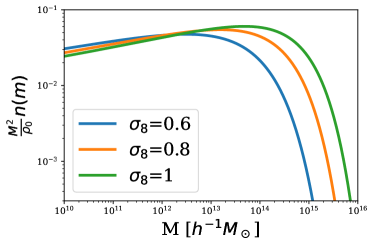
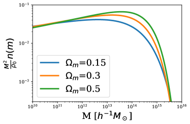
Figure 14: Variation of the collapsed fraction with $\sigma_{8}$ (left) and $\Omega_{\rm m}$ (right). The collapsed fraction increases slowly for low values of $\nu$, but then drops exponentially at high values; $\sigma_{8}$ changes the mass at which the transition to exponential behaviour occurs, while $\Omega_{\rm m}$ changes the sharpness of the transition.

Appendix D Parametric Dependence of the Formation Time

To understand the dependence of formation time on the cosmological parameters $\Omega_{\rm m}$ and $\sigma_{8}$, we consider the simplest, SC or Press-Schechter (PS) expression for $z_{50}$:

$$P_{PS}(z_{50}>z|M_{0},z_{0})\equiv\int_{M_{0}/2}^{M_{0}}\frac{M_{0}}{M}f_{PS}(M,z|M_{0},z_{0})dM\,,$$ (26)

where

$$\begin{gathered}f_{PS}(M_{1},z_{1}|M_{0},z_{0})dM_{1}=\frac{1}{\sqrt{2\pi}}\frac{\delta_{c}(z_{1})-\delta_{c}(z_{0})}{(S(M_{1})-S(M_{0}))^{3/2}}\\ \times\exp{\left(-\frac{\left(\delta_{c}(z_{1})-\delta_{c}(z_{0})\right)^{2}}{2(S(M_{1})-S(M_{0}))}\right)}dS_{1}\,.\end{gathered}$$ (27)

We can express $f_{PS}$ as a function of a single variable

$$D\nu\equiv\frac{\delta_{c}(z_{1})-\delta_{c}(z_{0})}{\sqrt{S(M_{1})-S(M_{0})}}\,,$$

as follows:

$$f_{PS}(M_{1},z_{1}|M_{0},z_{0})dM_{1}=\sqrt{\frac{2}{\pi}}\exp{\left(-\frac{(D\nu)^{2}}{2}\right)}|d(D\nu)|\,.$$ (28)

Thus, we see that the conditional probability has the same form as the unconditional one, but with the argument $D\nu$ rather than $\nu$.

The formation redshift distribution is proportional to the average value of the PMF between $M_{0}/2$ and $M_{0}$, and since the factor $M_{0}/M$ does not vary much over this range, it is also approximately equal to the conditional probability evaluated around the middle of the range. This probability $f_{PS}$ in turn goes as $\exp[-(D\nu)^{2}/2]$, so we expect the parametric dependence of $\langle z_{50}\rangle$ to resemble an inverted, logarithmic version of the dependence for $D\nu$.

Fig. 15 shows $\nu$ as a function of mass and redshift, while the top 4 panels of Fig. 16 show the value of $D\nu$ as a function of $z_{1}$ and mass fraction $M_{1}/M_{0}$, for various values of $M_{0}$ and $z_{0}$. We see that the shape of the $D\nu$ contours is generally similar to those for $\nu$, except when $z_{1}$ is close to $z_{0}$ (bottom of the plot), or when the mass fraction is close to 1 (right hand side of the plot).

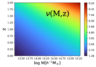
Figure 15: Peak height $\nu$ as a function of mass and redshift, in our fiducial ($\Omega_{\rm m}=0.3,\Omega_{\Lambda}=0.7$) cosmology.

The second set of 4 panels in Fig. 16 shows the value of the conditional probability. As expected, the conditional probability is similar to an inverse, logarithmic mapping of $D\nu$.

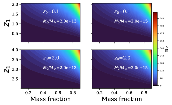
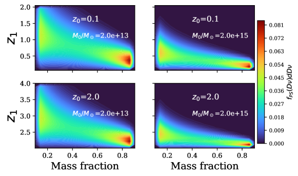
Figure 16: Top 4 panels: The variable $D\nu$ as a function of mass fraction $M_{1}/M_{0}$ and $z_{1}$, for the values of $(M_{0},z_{0})$ indicated, in our fiducial cosmology. Bottom 4 panels: corresponding conditional probability $f_{PS}(D\nu)d(D\nu)$.

Finally, we can consider the behaviour of $D\nu$ and the PMF in the $\Omega_{\rm m}$–$\sigma_{8}$ plane. The top 4 panels of Fig. 17 show the value of $D\nu$ in this plane, for the values of $(M_{0},z_{0})$ indicated, a mass fraction $M_{1}/M_{0}=0.5$, and $\Delta z=z_{1}-z_{0}=0.1$. The overall pattern is very similar to that of $\nu$ (cf. Fig. 1). The bottom four panels show the value of the PMF, for the same choices of $(z_{0},z_{1},M_{0},M_{1})$. Relative to the top panels, we see that the colour scale is inverted and logarithmic, as expected. The overall behaviour explains the shape of the contours in Fig. 5, and their relative orthogonality to abundance contours in the same plane.

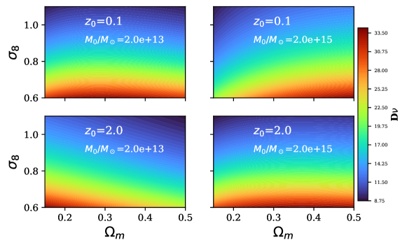
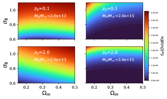
Figure 17: Top : $D\nu$ as a function of $\Omega_{\rm m}$ and $\sigma_{8}$, for the values of $(M_{0},z_{0})$ indicated, a mass fraction $M_{1}/M_{0}=0.5$, and $\Delta z=z_{1}-z_{0}=0.1$. Bottom: The corresponding conditional probability $f_{PS}(D\nu)d(D\nu)$ values as a function of $\Omega_{\rm m}$ and $\sigma_{8}$.

References

- Abazajian et al. (2019) Abazajian K., et al., 2019, arXiv e-prints, p. arXiv:1907.04473
- Abbott et al. (2020) Abbott T. M. C., et al., 2020, Phys. Rev. D, 102, 023509
- Abdullah et al. (2020) Abdullah M. H., Klypin A., Wilson G., 2020, ApJ, 901, 90
- Avila et al. (2014) Avila S., et al., 2014, MNRAS, 441, 3488
- Battye et al. (2015) Battye R. A., Charnock T., Moss A., 2015, Phys. Rev. D, 91, 103508
- Behroozi et al. (2013a) Behroozi P. S., Wechsler R. H., Wu H.-Y., 2013a, ApJ, 762, 109
- Behroozi et al. (2013b) Behroozi P. S., Wechsler R. H., Wu H.-Y., Busha M. T., Klypin A. A., Primack J. R., 2013b, ApJ, 763, 18
- Bocquet et al. (2016) Bocquet S., Saro A., Dolag K., Mohr J. J., 2016, MNRAS, 456, 2361
- Bocquet et al. (2020) Bocquet S., Heitmann K., Habib S., Lawrence E., Uram T., Frontiere N., Pope A., Finkel H., 2020, ApJ, 901, 5
- Böhringer et al. (2014) Böhringer H., Chon G., Collins C. A., 2014, A&A, 570, A31
- Bond et al. (1991) Bond J. R., Cole S., Efstathiou G., Kaiser N., 1991, ApJ, 379, 440
- Bullock et al. (2001) Bullock J. S., Kolatt T. S., Sigad Y., Somerville R. S., Kravtsov A. V., Klypin A. A., Primack J. R., Dekel A., 2001, MNRAS, 321, 559
- Carroll et al. (1992) Carroll S. M., Press W. H., Turner E. L., 1992, ARA&A, 30, 499
- Castro et al. (2021) Castro T., Borgani S., Dolag K., Marra V., Quartin M., Saro A., Sefusatti E., 2021, MNRAS, 500, 2316
- Chambers et al. (2020) Chambers K., Unions Team Including Pan-Starrs Team CFIS Team 2020, in American Astronomical Society Meeting Abstracts #235. p. 154.04
- Correa et al. (2015a) Correa C. A., Wyithe J. S. B., Schaye J., Duffy A. R., 2015a, MNRAS, 450, 1514
- Correa et al. (2015b) Correa C. A., Wyithe J. S. B., Schaye J., Duffy A. R., 2015b, MNRAS, 452, 1217
- Costanzi et al. (2021) Costanzi M., et al., 2021, Phys. Rev. D, 103, 043522
- DESI Collaboration et al. (2016) DESI Collaboration et al., 2016, arXiv e-prints, p. arXiv:1611.00036
- Debackere et al. (2021) Debackere S. N. B., Schaye J., Hoekstra H., 2021, MNRAS, 505, 593
- Despali et al. (2016) Despali G., Giocoli C., Angulo R. E., Tormen G., Sheth R. K., Baso G., Moscardini L., 2016, MNRAS, 456, 2486
- Diemand et al. (2007) Diemand J., Kuhlen M., Madau P., 2007, ApJ, 667, 859
- Diemer (2018) Diemer B., 2018, ApJS, 239, 35
- Douspis et al. (2019) Douspis M., Salvati L., Aghanim N., 2019, arXiv e-prints, p. arXiv:1901.05289
- Drakos et al. (2019a) Drakos N. E., Taylor J. E., Berrouet A., Robotham A. S. G., Power C., 2019a, MNRAS, 487, 993
- Drakos et al. (2019b) Drakos N. E., Taylor J. E., Berrouet A., Robotham A. S. G., Power C., 2019b, MNRAS, 487, 1008
- Eisenstein & Hu (1998) Eisenstein D. J., Hu W., 1998, ApJ, 496, 605
- Evrard et al. (1993) Evrard A. E., Mohr J. J., Fabricant D. G., Geller M. J., 1993, ApJ, 419, L9
- Gao et al. (2004) Gao L., White S. D. M., Jenkins A., Stoehr F., Springel V., 2004, MNRAS, 355, 819
- Gao et al. (2005) Gao L., Springel V., White S. D. M., 2005, MNRAS, 363, L66
- Gill et al. (2004) Gill S. P. D., Knebe A., Gibson B. K., 2004, MNRAS, 351, 399
- Giocoli et al. (2007) Giocoli C., Moreno J., Sheth R. K., Tormen G., 2007, MNRAS, 376, 977
- Giocoli et al. (2012) Giocoli C., Tormen G., Sheth R. K., 2012, MNRAS, 422, 185
- Groener et al. (2016) Groener A. M., Goldberg D. M., Sereno M., 2016, MNRAS, 455, 892
- Harker et al. (2006) Harker G., Cole S., Helly J., Frenk C., Jenkins A., 2006, MNRAS, 367, 1039
- Henry et al. (2009) Henry J. P., Evrard A. E., Hoekstra H., Babul A., Mahdavi A., 2009, ApJ, 691, 1307
- Heymans et al. (2021) Heymans C., et al., 2021, A&A, 646, A140
- Jenkins et al. (2001) Jenkins A., Frenk C. S., White S. D. M., Colberg J. M., Cole S., Evrard A. E., Couchman H. M. P., Yoshida N., 2001, MNRAS, 321, 372
- Kacprzak et al. (2016) Kacprzak T., et al., 2016, MNRAS, 463, 3653
- Klypin et al. (2011) Klypin A. A., Trujillo-Gomez S., Primack J., 2011, ApJ, 740, 102
- Knebe et al. (2011) Knebe A., et al., 2011, MNRAS, 415, 2293
- Knollmann & Knebe (2009) Knollmann S. R., Knebe A., 2009, ApJS, 182, 608
- LSST Science Collaboration et al. (2009) LSST Science Collaboration et al., 2009, arXiv e-prints, p. arXiv:0912.0201
- Lacey & Cole (1993) Lacey C., Cole S., 1993, MNRAS, 262, 627
- Ludlow et al. (2013) Ludlow A. D., et al., 2013, MNRAS, 432, 1103
- Ludlow et al. (2014) Ludlow A. D., Navarro J. F., Angulo R. E., Boylan-Kolchin M., Springel V., Frenk C., White S. D. M., 2014, MNRAS, 441, 378
- Macciò et al. (2007) Macciò A. V., Dutton A. A., van den Bosch F. C., Moore B., Potter D., Stadel J., 2007, MNRAS, 378, 55
- Mantz et al. (2010) Mantz A., Allen S. W., Rapetti D., Ebeling H., 2010, MNRAS, 406, 1759
- Mo et al. (2010) Mo H., van den Bosch F., White S., 2010, Galaxy Formation and Evolution. Cambridge University Press, doi:10.1017/CBO9780511807244
- Mohr et al. (1995) Mohr J. J., Evrard A. E., Fabricant D. G., Geller M. J., 1995, ApJ, 447, 8
- Navarro et al. (1997) Navarro J. F., Frenk C. S., White S. D. M., 1997, ApJ, 490, 493
- Nelson et al. (2019) Nelson D., et al., 2019, Computational Astrophysics and Cosmology, 6, 2
- Pillepich et al. (2012) Pillepich A., Porciani C., Reiprich T. H., 2012, MNRAS, 422, 44
- Planck Collaboration et al. (2020) Planck Collaboration et al., 2020, A&A, 641, A6
- Power et al. (2012) Power C., Knebe A., Knollmann S. R., 2012, MNRAS, 419, 1576
- Press & Schechter (1974) Press W. H., Schechter P., 1974, ApJ, 187, 425
- Richstone et al. (1992) Richstone D., Loeb A., Turner E. L., 1992, ApJ, 393, 477
- Riess et al. (2019) Riess A. G., Casertano S., Yuan W., Macri L. M., Scolnic D., 2019, ApJ, 876, 85
- Rodriguez-Gomez et al. (2015) Rodriguez-Gomez V., et al., 2015, MNRAS, 449, 49
- Sartoris et al. (2016) Sartoris B., et al., 2016, MNRAS, 459, 1764
- Sheth & Tormen (1999) Sheth R. K., Tormen G., 1999, MNRAS, 308, 119
- Sheth & Tormen (2002) Sheth R. K., Tormen G., 2002, MNRAS, 329, 61
- Srisawat et al. (2013) Srisawat C., et al., 2013, MNRAS, 436, 150
- Taylor (2011) Taylor J. E., 2011, Advances in Astronomy, 2011, 604898
- Taylor & Babul (2005) Taylor J. E., Babul A., 2005, MNRAS, 364, 515
- Tinker et al. (2008) Tinker J., Kravtsov A. V., Klypin A., Abazajian K., Warren M., Yepes G., Gottlöber S., Holz D. E., 2008, ApJ, 688, 709
- To et al. (2021) To C., et al., 2021, Phys. Rev. Lett., 126, 141301
- Velliscig et al. (2014) Velliscig M., van Daalen M. P., Schaye J., McCarthy I. G., Cacciato M., Le Brun A. M. C., Dalla Vecchia C., 2014, MNRAS, 442, 2641
- Verde et al. (2019) Verde L., Treu T., Riess A. G., 2019, Nature Astronomy, 3, 891
- Wang et al. (2020) Wang K., Mao Y.-Y., Zentner A. R., Lange J. U., van den Bosch F. C., Wechsler R. H., 2020, MNRAS, 498, 4450
- Watson et al. (2013) Watson W. A., Iliev I. T., D’Aloisio A., Knebe A., Shapiro P. R., Yepes G., 2013, MNRAS, 433, 1230
- Wechsler et al. (2002) Wechsler R. H., Bullock J. S., Primack J. R., Kravtsov A. V., Dekel A., 2002, ApJ, 568, 52
- Wechsler et al. (2006) Wechsler R. H., Zentner A. R., Bullock J. S., Kravtsov A. V., Allgood B., 2006, ApJ, 652, 71
- Wong & Taylor (2012) Wong A. W. C., Taylor J. E., 2012, ApJ, 757, 102
- Zhang et al. (2008) Zhang J., Fakhouri O., Ma C.-P., 2008, MNRAS, 389, 1521
- Zhao et al. (2003) Zhao D. H., Jing Y. P., Mo H. J., Börner G., 2003, ApJ, 597, L9
- Zhao et al. (2009) Zhao D. H., Jing Y. P., Mo H. J., Börner G., 2009, ApJ, 707, 354
- de Haan et al. (2016) de Haan T., et al., 2016, ApJ, 832, 95
- van den Bosch (2002) van den Bosch F. C., 2002, MNRAS, 331, 98