Motility switching and front-back synchronisation in polarized cells

Abstract

The combination of protrusions and retractions in the movement of polarized cells leads to understand the effect of possible synchronisation between the two ends of the cells. This synchronisation, in turn, could lead to different dynamics such as normal and fractional diffusion. Departing from a stochastic single cell trajectory, where a “memory effect” induces persistent movement, we derive a kinetic-renewal system at the mesoscopic scale. We investigate various scenarios with different levels of complexity, where the two ends of the cell move either independently or with partial or full synchronisation. We study the relevant macroscopic limits where we obtain diffusion, drift-diffusion or fractional diffusion, depending on the initial system. This article clarifies the form of relevant macroscopic equations that describe the possible effects of synchronised movement in cells, and sheds light on the switching between normal and fractional diffusion.

Introduction

Mathematical modelling of cell motility has been largely studied, specially through the use of partial differential equations (PDEs). Depending on the biological context, cell trajectories can be described by a persistent random walk [21], where the individual tends to keep moving in the same direction as observed in [15, 10]. Often, directional persistence is also described as a correlated random walk where the direction of previous steps influences the direction of next ones.

This type of movement was studied in [12] where, due to the synchronisation of protrusions and retractions in the front and back of metastatic cells, the authors observed a strong presence of long runs, interspersed by a sequence of short steps. These characteristics are analogous to Lévy walk trajectories, where the probability of a long run, i.e. a trajectory in the same direction for a long time, is non negligible. It was also observed that in non-metastatic cells the front and back movements are independent and then they follow a classical random walk. In contrast to a Brownian motion, where the distribution of the individuals’ trajectories follows a Gaussian, Lévy walk trajectories asymptotically follow a power-law distribution [19, 30]. Moreover, while for the Brownian case the mean square displacement $\langle x^{2}\rangle$ grows linearly with respect to time ($\langle x^{2}\rangle\sim t$), for the Lévy walk case we have $\langle x^{2}\rangle\sim t^{\zeta}$ where $\zeta\in(1,2)$. The exponent $\zeta=2$ corresponds to ballistic transport while $\zeta=1$ corresponds to normal diffusion. When $\zeta\in(1,2)$ we are in the superdiffusive regime. For the ubiquitous appearance of Lévy walk models in biological systems we refer to [1, 11, 14] at the cellular level, [29, 27, 25, 7, 26] for animals and [23, 24] for humans.

In this work, we start from the most general description: when front and back can make independent, non-synchronised steps to the right and to the left. In this setting, the model records the persistence time in each direction, thus leading to a complex system which can better be understood in terms of cell elongation and movement of the center of gravity.

To reduce the complexity, we assume that the cell length is fixed at the mesoscopic scale under investigation; the model is now amenable to multi-scale analysis and depending on the switching rates of both ends, we compute a diffusion coefficient at the macroscopic scale. Such a model with a given cell length can also be derived from the full system assuming fast switches in the dynamics of cell elongation compared to those for the movement. We also investigate the synchronisation between back and front, where we can observe a full range of behaviours. With low persistence, normal diffusion occurs, possibly with a drift and explicit formulas are computed. They show the possibility of a “backward diffusion” regime which can be interpreted as instability of the constant steady state at the kinetic (mesoscopic) scale. More interesting is when persistence is higher, then fractional diffusion occurs exhibiting the phenomena of long excursions which motivates our study.

When going back to individual cell (microscopic) dynamics, we perform numerical simulations and, as explained earlier, the long time behaviour quantifies the fractional diffusion in accordance to the developed theory.

To motivate our modelling, we are going to describe, based on biological evidence presented in [12], two systems where none or full synchronisation of front and back leads to diffusive or superdiffusive dynamics, respectively.

Cell persistent movement through front-back synchronisation

As previously introduced, the full synchronisation in space and time of the front and back movements of cells leads to Lévy walk dynamics, as observed in [12] for the case of metastatic cancer cells. On the other hand, when the cells’ front and back movements are independent, the trajectories follow a normal diffusion.

The synchronisation is translated into a persistence of the movement in a given direction. This means that at a given time step, the ends of the cell move forward or backwards simultaneously. The non-synchronisation is the result of independent movements in the front and back which might result in an intermittent cell movement pattern, where the cell length can vary. Hence, we assume that when the steps are not independent, and the cell keeps some “memory” of previous steps (non-Markovian process), the distribution of persistence length corresponds to a power-law and the movement is described by a Lévy walk. If the steps are independent, then the trajectories correspond to a diffusive movement. A more detailed description of this persistent and non-persistent movement is given in Section 1 (see also Supplementary Information in [12]).

The aim of this article is to derive macroscopic equations that characterise these dynamics, starting from a kinetic description of the individual movement. To study this behaviour we propose the following setting. We consider that a cell is approximated by a one dimensional system of two identical point masses attached by an elastic cord. Each point mass is going to represent the front and back of the cell and the elastic cord represents the cell length. We aim to describe the trajectories of the whole system as in Figure 1. Each mass is considered as a material point that takes discrete (in space and time) infinitesimally small steps to the left or to the right with a certain probability. For the non-synchronisation case (Figure 1a) we consider the independent movement of the front (represented by $y$) and back (represented by $x$) and the cell length change, where $\ell_{c}$ is the length at rest (see Subsection 2.1). While studying the synchronised movement leading to superdiffusion, since the front and back simultaneously move in the same direction at each time, we only consider the change in position of the centre of mass, represented by $x$ in Figure 1b. Since the cell length is fixed in this case, we do not take it into account.

Outline of the paper

In Section 1 we present a detailed description of the individual movement as well as the main modelling assumptions. In Section 2 we introduce a general model where front and back movements are not synchronised. We also discuss some general notions as conservation of particles and realistic cell length for the model. Section 3 presents a simplified version of the previous model where we fix the cell length at the mesoscopic scale. We derive macroscopic equations depending on the switching rates at the ends of the cell. This model is also obtained by considering a fast switching dynamics in the full system as described in Subsection 3.1. In Section 4 we consider the system with synchronised front and back movement. We study the diffusive regime, when the persistence is low, and the superdiffusive regime in the opposite case (Section 5). Here we also show the possibility of a “backwards diffusion” regime. Finally, in Section 6 we perform numerical simulations at the individual level to compare with the developed theory.

1 Description of mathematical model

Front-back non-synchronisation

In this case, the front and back movements are independent but with probabilities sampled from the same probability distribution. We consider that the front ($y$) gives a step $k_{y}$ of size $\delta$ at a given time $\tau$, and similarly for the back $x$. The cell length is given by $|y-x|$ where $\ell_{c}$ denotes the equilibrium length. If the whole system is moving to the right initially, the cell front is allowed to reverse direction and move to $y-\delta$ with probability $q_{k_{y}}=\tau p_{k_{y}}$ or it can keep moving in the same direction with probability $\tilde{q}_{k_{y}}=1-\tau p_{k_{y}}$. Similarly, the back of the cell can move in the positive direction $x+\delta$ with probability $\tilde{q}_{k_{x}}=1-\tau p_{k_{x}}$ or reverse direction with probability $q_{k_{x}}=\tau p_{k_{x}}$. The length of the cell varies in a specific range so that we preserve the physical properties, as described later in Section 2.1.

Front-back synchronisation

For this case, since the front and back of the cell move simultaneously, i.e. at each time step they move to the left or to the right one step size with the same probability, the cell length is fixed at all times and we can consider the whole system as a point particle. The elastic cord can be considered as a solid road of fixed length and we study the movement of the center of mass only as in Figure 1b.

Analogous to the previous description, if we assume that the system is initially moving to the right, then it can reverse direction to $x-\delta$ with probability $q_{k}=\tau p_{k}$ or it can keep moving forward to $x+\delta$ with a probability $\tilde{q}_{k}=1-\tau p_{k}$. Every time the cell changes direction we set $k=0$ and we start counting again. The probability of keep moving without reversing will algebraically decrease with $k$.

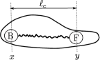
(a) Non-synchronisation.

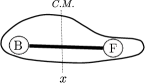
(b) Synchronisation

Figure 1: Schematics of the front-back cell movement.

Note: From now on, we use the notation $p_{k}$ when $k$ is discrete (see also Subsection 6.1) and $p(k)$ when $k$ is continuous.

Reversing direction probability

As described earlier, the rate at which the cell changes direction from left to right movement, given by $p_{k}$, depends on the number of steps $k$ given in that direction. The reversing rate is associated with a probability $\psi(k)$, which is given by

$$\psi(k)=e^{-\int_{0}^{k}p(k^{*})\mathop{}\!\mathrm{d}k^{*}}\ .$$ (1)

This function $\psi$ is often referred to as the survival probability, i.e., it gives the probability that the event of interest, in this case the reverse in direction, has not occurred for $k$ steps. Equation (1) means that the probability of moving for $k$ steps without changing is equal to the exponential of the cumulative reversing frequency. As indicated in [12], for the case of metastatic cells this probability decays algebraically with $k$, therefore, here we consider that

$$\psi(k)=\Bigl{(}\frac{k_{0}}{k_{0}+k}\Bigr{)}^{\mu}\ \ \ \textnormal{for}\ \ \mu\in(1,3)\ .$$ (2)

The reversing direction rate $p(k)$ can also be expressed as the ratio

$$p(k)=\frac{\phi(k)}{\psi(k)}=\frac{-\partial_{k}\psi(k)}{\psi(k)}\ ,$$ (3)

where $\phi(k)$ is a probability density function. The above expression means that the reversing rate at step $k$ equals the density of the event divided by the probability of keep moving in the same direction for $k$ steps.

2 Non-synchronised movement description

We assume that the probabilities of the protrusions and retractions are independent from each other and therefore we have four different scenarios as in Figure 2. We denote by $\alpha(t,x,y,k_{x},k_{y})$ and $\beta(t,x,y,k_{x},k_{y})$ the cells that are moving to the right and left, respectively, and by $\delta(t,x,y,k_{x},k_{y})$ and $\gamma(t,x,y,k_{x},k_{y})$ the cells that only change their length by elongation and contraction. Moreover, the steps at the cell front, denoted by $k_{y}$, are independent from the steps at the back, $k_{x}$, and consequently, we have to take into account the rates $p^{\alpha}_{x}$, $p^{\alpha}_{y}$, $p^{\beta}_{x}$, $p^{\beta}_{y}$, $p^{\gamma}_{x}$, $p^{\gamma}_{y}$, $p^{\delta}_{x}$ and $p^{\delta}_{y}$. These rates do not only depend on $k_{x}$ and $k_{y}$ but also on the distance $|x-y|$ to preserve the cell physical size, as we discuss in Section 2.1. When the front and back of the cell change direction simultaneously, $p_{x}=p_{y}$, we denote the corresponding switching rates as $p^{\alpha},\ p^{\beta},\ p^{\gamma},\ p^{\delta}$.

Note that cases (a) and (b) in Figure 2 are analogous to the synchronisation case later discussed in Section 4.

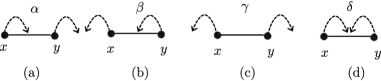
Figure 2: Non-synchronised movement where the cell moves to the right (a), to the left (b) or changes its length by stretching (c) and shrinking (d).

In full generality, the number density of each cell population is described by the following systems coupled through the boundary terms,

$$\begin{cases}&(\partial_{t}+v\partial_{x}+v\partial_{y}+\partial_{k_{x}}+\partial_{k_{y}})\alpha=-(p_{x}^{\alpha}+p_{y}^{\alpha})\alpha{-p^{\alpha}\alpha}\ ,\\ &\alpha(t,x,y,k_{x}=0,k_{y})=\int_{0}^{\infty}p_{x}^{\gamma}\gamma\mathop{}\!\mathrm{d}k_{x}\ ,\\ &\alpha(t,x,y,k_{x},k_{y}=0)=\int_{0}^{\infty}p_{y}^{\delta}\delta\mathop{}\!\mathrm{d}k_{y}\ ,\\ &\alpha(t,x,y,k_{x}=0,k_{y}=0)=\int_{0}^{\infty}\int_{0}^{\infty}p^{\beta}\beta\mathop{}\!\mathrm{d}k_{x}\mathop{}\!\mathrm{d}k_{y}\ ,\end{cases}$$ (4)

$$\begin{cases}&(\partial_{t}-v\partial_{x}-v\partial_{y}+\partial_{k_{x}}+\partial_{k_{y}})\beta=-(p_{x}^{\beta}+p^{\beta}_{y})\beta{-p^{\beta}\beta}\ ,\\ &\beta(t,x,y,k_{x}=0,k_{y})=\int_{0}^{\infty}p_{x}^{\delta}\delta\mathop{}\!\mathrm{d}k_{x}\ ,\\ &\beta(t,x,y,k_{x},k_{y}=0)=\int_{0}^{\infty}p_{y}^{\gamma}\gamma\mathop{}\!\mathrm{d}k_{y}\ ,\\ &\beta(t,x,y,k_{x}=0,k_{y}=0)=\int_{0}^{\infty}\int_{0}^{\infty}p^{\alpha}\alpha\mathop{}\!\mathrm{d}k_{x}\mathop{}\!\mathrm{d}k_{y}\ ,\end{cases}$$ (5)

$$\begin{cases}&(\partial_{t}-v\partial_{x}+v\partial_{y}+\partial_{k_{x}}+\partial_{k_{y}})\gamma=-(p_{x}^{\gamma}+p_{y}^{\gamma})\gamma{-p^{\gamma}\gamma}\ ,\\ &\gamma(t,x,y,k_{x}=0,k_{y})=\int_{0}^{\infty}p_{x}^{\alpha}\alpha\mathop{}\!\mathrm{d}k_{x}\ ,\\ &\gamma(t,x,y,k_{x},k_{y}=0)=\int_{0}^{\infty}p_{y}^{\beta}\beta\mathop{}\!\mathrm{d}k_{y}\ ,\\ &\gamma(t,x,y,k_{x}=0,k_{y}=0)=\int_{0}^{\infty}\int_{0}^{\infty}p^{\delta}\delta\mathop{}\!\mathrm{d}k_{x}\mathop{}\!\mathrm{d}k_{y}\ ,\end{cases}$$ (6)

$$\begin{cases}&(\partial_{t}+v\partial_{x}-v\partial_{y}+\partial_{k_{x}}+\partial_{k_{y}})\delta=-(p_{x}^{\delta}+p^{\delta}_{y})\delta{-p^{\delta}\delta}\ ,\\ &\delta(t,x,y,k_{x}=0,k_{y})=\int_{0}^{\infty}p_{x}^{\beta}\beta\mathop{}\!\mathrm{d}k_{x}\ ,\\ &\delta(t,x,y,k_{x},k_{y}=0)=\int_{0}^{\infty}p_{y}^{\alpha}\alpha\mathop{}\!\mathrm{d}k_{y}\ ,\\ &\delta(t,x,y,k_{x}=0,k_{y}=0)=\int_{0}^{\infty}\int_{0}^{\infty}p^{\gamma}\gamma\mathop{}\!\mathrm{d}k_{x}\mathop{}\!\mathrm{d}k_{y}\ .\end{cases}$$ (7)

The above systems of equations describe the different jumping combinations represented in Figure 2. For instance, in the case of population $\alpha$, if $x$ changes direction with certain rate $p_{x}^{\alpha}$, then we have a transition from population $\alpha$ to $\gamma$ (Figure 2 (a)$\to$(c)), which is given by $\gamma(t,x,y,k_{x}=0,k_{y})$. Similarly, if $y$ changes direction in population $\alpha$ we have a change from $\alpha$ to $\delta$, and the individuals that leave population $\alpha$ appear in $\delta(t,x,y,k_{x},k_{y}=0)$. The reverse process also happens and transitions from population $\gamma$ to $\alpha$ (cells appear at $\alpha(t,x,y,k_{x}=0,k_{y})$) and from $\delta$ to $\alpha$ (cells appear at $\alpha(t,x,y,k_{x},k_{y}=0)$) are also considered. When the jumping direction changes at $x$ and $y$ simultaneously then it always happens that populations switch directly from $\alpha\longleftrightarrow\beta$ and $\gamma\longleftrightarrow\delta$.

Notation: For simplicity of notation, in the rest of the paper we use

$$\iint\limits(\cdot)=\int_{0}^{\infty}\int_{0}^{\infty}(\cdot)\mathop{}\!\mathrm{d}k_{x}\mathop{}\!\mathrm{d}k_{y}\ .$$

In the following we are going to check some physical properties that the systems (4)-(7) must satisfy.

Coordinates of the center of mass and cell elongation

At a first stage, a desirable property is that cell polarization is preserved, that means $x<y$ all along the movement assuming it is true initially. To examine the conditions which enforce this property it is easier to use the coordinates of the center of mass and the distance between back and front. For that we let $\frac{x+y}{2}=X$ and $y-x=z$, the cell length. From now on, and for simplicity in the notation, we keep the same functions $\alpha,\ \beta,\ \gamma,\ \delta$ that will depend on the new variables $(t,X,z,k_{x},k_{y})$. From the system (4)-(7) we get

$$(\partial_{t}+2v\partial_{X}+\partial_{k_{x}}+\partial_{k_{y}}){\alpha} =-(p_{x}^{\alpha}+p^{\alpha}_{y}){\alpha}-p^{\alpha}{\alpha}\ ,$$ (8)

$$(\partial_{t}-2v\partial_{X}+\partial_{k_{x}}+\partial_{k_{y}}){\beta} =-(p_{x}^{\beta}+p_{y}^{\beta}){\beta}-p^{\beta}{\beta}\ ,$$ (9)

$$(\partial_{t}+v\partial_{z}+\partial_{k_{x}}+\partial_{k_{y}}){\gamma} =-(p_{x}^{\gamma}+p_{y}^{\gamma}){\gamma}-p^{\gamma}{\gamma}\ ,$$ (10)

$$(\partial_{t}-\ v\partial_{z}+\partial_{k_{x}}+\partial_{k_{y}}){\delta} =-(p_{x}^{\delta}+p_{y}^{\delta}){\delta}-p^{\delta}{\delta}\ ,$$ (11)

with the boundary conditions in $k_{x}$, $k_{y}$,

$${\alpha}(\cdot,k_{x}=0,k_{y})=\int_{0}^{\infty}p_{x}^{\gamma}{\gamma}\mathop{}\!\mathrm{d}k_{x}\ ,\quad{\alpha}(\cdot,k_{x},k_{y}=0)=\int_{0}^{\infty}p_{y}^{\delta}{\delta}\mathop{}\!\mathrm{d}k_{y}\ ,\quad{\alpha}(\cdot,k_{x}=0,k_{y}=0)=\iint\limits p^{\beta}{\beta}\ ,$$ (12)

$${\beta}(\cdot,k_{x}=0,k_{y})=\int_{0}^{\infty}p_{x}^{\delta}{\delta}\mathop{}\!\mathrm{d}k_{x}\ ,\quad{\beta}(\cdot,k_{x},k_{y}=0)=\int_{0}^{\infty}p_{y}^{\gamma}{\gamma}\mathop{}\!\mathrm{d}k_{y}\ ,\quad{\beta}(\cdot,k_{x}=0,k_{y}=0)=\iint\limits p^{\alpha}{\alpha}\ ,$$ (13)

$${\gamma}(\cdot,k_{x}=0,k_{y})=\int_{0}^{\infty}p_{x}^{\alpha}{\alpha}\mathop{}\!\mathrm{d}k_{x}\ ,\quad{\gamma}(\cdot,k_{x},k_{y}=0)=\int_{0}^{\infty}p_{y}^{\beta}{\beta}\mathop{}\!\mathrm{d}k_{y}\ ,\quad{\gamma}(\cdot,k_{x}=0,k_{y}=0)=\iint\limits p^{\delta}{\delta}\ ,$$ (14)

$${\delta}(\cdot,k_{x}=0,k_{y})=\int_{0}^{\infty}p_{x}^{\beta}{\beta}\mathop{}\!\mathrm{d}k_{x}\ ,\quad{\delta}(\cdot,k_{x},k_{y}=0)=\int_{0}^{\infty}p_{y}^{\alpha}{\alpha}\mathop{}\!\mathrm{d}k_{y}\ ,\quad{\delta}(\cdot,k_{x}=0,k_{y}=0)=\iint\limits p^{\gamma}{\gamma}\ .$$ (15)

Here $(\cdot)$ denotes the dependence on $(t,X,z)$. In order to guarantee that $z>0$ is preserved, we also need to ensure that ${\delta}(X,z=0,k_{x},k_{y})=0$ (similarly $\gamma(X,z=0,k_{x},k_{y})=0$), which means that the jump rate $p^{\delta}_{x}+p^{\delta}_{y}\to\infty$ as $z\to 0$ and $\int_{0}^{\cdot}(p^{\delta}_{x}+p^{\delta}_{y})(z)\mathop{}\!\mathrm{d}z=\infty$. Using the notation in (19), this means that $\int_{0}^{\cdot}\mu_{\delta}(z)\mathop{}\!\mathrm{d}z=\infty$.

Conservation of particles

Integrating with respect to $k_{x}$ and $k_{y}$ we define the macroscopic density

$$\bar{{\alpha}}(t,X,z)=\iint\limits{\alpha}(\cdot,k_{x},k_{y})\ ,$$ (16)

and similarly for $\bar{\beta},\ \bar{\gamma}$ and $\bar{\delta}$. Moreover, integrating with respect to $k_{x}$ and $k_{y}$ equations (8)-(11) and adding them together we obtain the following macroscopic conservation equation

$$\partial_{t}(u+w)+2v\partial_{X}j+v\partial_{z}m=0\ .$$ (17)

Here $u(t,X,z)=\bar{{\alpha}}+\bar{{\beta}}$ is the moving population, $w(t,X,z)=\bar{{\gamma}}+\bar{{\delta}}$ is the resting population, $j(t,X,z)=\bar{{\alpha}}-\bar{{\beta}}$ is the mean direction of motion and $m(t,X,z)=\bar{{\gamma}}-\bar{{\delta}}$ is the mean extension rate.

2.1 Biologically relevant switching probabilities

The switching rate is not going to depend only on the persisting steps $k_{x}$ and $k_{y}$ but also on the cell length $z$. Using (2) and (3) we can write the general expression

$$p(k)=\frac{\mu}{1+k}\ .$$ (18)

For the non-synchronised movement this rate is given by, for population $\alpha$ (and similarly for the rest),

$$p_{x}^{\alpha}(k_{x})=\frac{\mu_{\alpha}(z)}{1+k_{x}}\ ,\qquad p_{y}^{\alpha}(k_{y})=\frac{\mu_{\alpha}(z)}{1+k_{y}}\ .$$ (19)

The dependence of $\mu$ on $z$ guarantees that we keep a realistic cell length as we will discuss below. For the synchronised case, since the cell does not change shape, we consider the switching rate given by (18).

As described in [12] the length of a cell can only vary in a certain range. Considering that the resting length is $\ell_{c}=|y-x|$, we define $L_{\textnormal{max}}=3.5\ell_{c}$ and $L_{\textnormal{min}}=0.5\ell_{c}$ and the switching rates satisfy the following properties,

$$p_{x}^{\alpha}=\begin{cases}\epsilon&\textnormal{if}\ z\gg L_{\textnormal{max}}\ ,\\ \frac{\mu_{\alpha}(z)}{1+k_{x}}&\textnormal{if}\ z\ll L_{\textnormal{min}}\ ,\end{cases}\ \ \ \ p_{y}^{\alpha}=\begin{cases}\frac{\mu_{\alpha}(z)}{1+k_{y}}&\textnormal{if}\ z\gg L_{\textnormal{max}}\ ,\\ \epsilon&\textnormal{if}\ z\ll L_{\textnormal{min}}\ ,\end{cases}$$ (20)

$$p_{x}^{\beta}=\begin{cases}\frac{\mu_{\beta}(z)}{1+k_{x}}&\textnormal{if}\ z\gg L_{\textnormal{max}}\ ,\\ \epsilon&\textnormal{if}\ z\ll L_{\textnormal{min}}\ ,\end{cases}\ \ \ \ p_{y}^{\beta}=\begin{cases}\epsilon&\textnormal{if}\ z\gg L_{\textnormal{max}}\ ,\\ \frac{\mu_{\beta}(z)}{1+k_{y}}&\textnormal{if}\ z\ll L_{\textnormal{min}}\ ,\end{cases}$$ (21)

and finally,

$$p^{\gamma}_{x}=\begin{cases}\frac{\mu_{\gamma}(z)}{1+k_{x}}&\textnormal{if}\ z\gg L_{\textnormal{max}}\ ,\\ \epsilon&\textnormal{if}\ z\ll L_{\textnormal{min}}\ ,\end{cases}\ \ \ \ p^{\gamma}_{y}=\begin{cases}\frac{\mu_{\gamma}(z)}{1+k_{y}}&\textnormal{if}\ z\gg L_{\textnormal{max}}\ ,\\ \epsilon&\textnormal{if}\ z\ll L_{\textnormal{min}}\ ,\end{cases}$$ (22)

$$p^{\delta}_{x}=\begin{cases}\epsilon&\textnormal{if}\ z\gg L_{\textnormal{max}}\ ,\\ \frac{\mu_{\delta}(z)}{1+k_{x}}&\textnormal{if}\ z\ll L_{\textnormal{min}}\ ,\end{cases}\ \ \ \ p^{\delta}_{y}=\begin{cases}\epsilon&\textnormal{if}\ z\gg L_{\textnormal{max}}\ ,\\ \frac{\mu_{\delta}(z)}{1+k_{y}}&\textnormal{if}\ z\ll L_{\textnormal{min}}\ .\end{cases}$$ (23)

Here $\epsilon$ is a small parameter. Let us take for instance the case when cells are moving right (population $\alpha$). In the limit when $z\gg L_{\textnormal{max}}$, since we want to preserve the physical length of the cell, the front has to change direction with a higher rate ($p_{y}^{\alpha}$) while the back should keep moving in the same direction (small $p_{x}^{\alpha}$). On the other hand, in the limit when $z\ll L_{\textnormal{min}}$ the back of the cell has to switch direction ($p_{x}^{\alpha}$) while the front should keep moving without changing (small $p_{y}^{\alpha}$). The opposite happens when the cell is moving to the left (population $\beta$).

For the case when the cell is at rest ($\gamma$ and $\delta$), if $z\gg L_{\textnormal{max}}$ for the case of the population $\gamma$, the switching rate has to be very high at both ends so that the cell recovers the resting length $\ell_{c}$. If $z\ll L_{\textnormal{min}}$, then $p^{\gamma}_{x}$, $p_{y}^{\gamma}$ are very small. The opposite happens in the case of the population $\delta$.

3 Simplified system with resting population

The systems (8)-(11) are very complex to analyse since they involve different dynamics such as left and right movement for four different populations, and additionally, the change in cell length. Therefore, in this section we consider a simplified model of three populations: cells moving left ($\beta$), cells moving right ($\alpha$) and resting cells ($\gamma_{0}$). The population $\gamma_{0}$ represents the average of the populations $\gamma$ and $\delta$ described before assuming the mean cell length is constant, thus ignoring the variable $z$. The dynamics are described now by

$$\begin{cases}&\varepsilon^{2}\partial_{t}\alpha_{\varepsilon}+\varepsilon v\partial_{x}\alpha_{\varepsilon}+\partial_{k}\alpha_{\varepsilon}=-{p}(k)\alpha_{\varepsilon}\ ,\\ &\alpha_{\varepsilon}(t,0,x)=\zeta^{\beta}\int_{0}^{\infty}{p}(k)\beta_{\varepsilon}\mathop{}\!\mathrm{d}k+\zeta^{\gamma}\gamma^{\varepsilon}_{0}(t,x,0)\ ,\end{cases}$$ (24)

$$\begin{cases}&\varepsilon^{2}\partial_{t}\beta_{\varepsilon}-\varepsilon v\partial_{x}\beta_{\varepsilon}+\partial_{k}\beta_{\varepsilon}=-{p}(k)\beta_{\varepsilon}\ ,\\ &\beta_{\varepsilon}(t,0,x)=\zeta^{\alpha}\int_{0}^{\infty}{p}(k)\alpha_{\varepsilon}\mathop{}\!\mathrm{d}k+(1-\zeta^{\gamma})\gamma^{\varepsilon}_{0}(t,x,0)\ ,\end{cases}$$ (25)

$$\begin{cases}&\varepsilon^{2}\partial_{t}\gamma^{\varepsilon}_{0}-\partial_{k}\gamma_{0}^{\varepsilon}=(1-\zeta^{\alpha}){p}(k)\alpha_{\varepsilon}+(1-\zeta^{\beta}){p}(k)\beta_{\varepsilon}\ .\end{cases}$$ (26)

The switching rate ${p}(k)$ describes both the change in direction of the center of mass and transition to rest state $\gamma_{0}$ where memory is gradually lost. This replaces the movement of the front and the back of the cell as in Section 2 and is given by (18). Since we are not considering front and back movements then $\alpha$, $\beta$ and $\gamma_{0}$ depend only on $(t,x,k)$. In the above system, $\zeta\in(0,1)$ is a probability and note that we have introduced a diffusive scaling $(t,x)\mapsto(\bar{t}/\varepsilon^{2},\bar{x}/\varepsilon)$. The individuals from population $\alpha$ that switch direction with rate ${p}(k)$ either start moving in the opposite direction with probability $\zeta^{\alpha}$, represented by the first term in $\beta_{\varepsilon}(t,x,0)$, or they go into a resting phase with probability $1-\zeta^{\alpha}$, given by the first term in the right hand side of (26). A similar dynamic is followed by individuals in population $\beta$. On the other hand, individuals that are at rest, population $\gamma_{0}$, start to move to the right, with probability $\zeta^{\gamma}$, or to the left with probability $1-\zeta^{\gamma}$.

As for the systems (4)-(7), we can easily check that (24)-(26) preserves the number density of individuals.

When the rate ${p}(k)$ is large enough for large $k$, more precisely when $ke^{-\int_{0}^{k}{p}(k^{*})\mathop{}\!\mathrm{d}k^{*}}$ is integrable, then the large scale dynamics is normal diffusion. To explain this, we define the survival probability $\psi$ as

$$\psi(k)=Ze^{-\int_{0}^{k}{p}(k^{*})\mathop{}\!\mathrm{d}k^{*}},\qquad Z^{-1}:=\int_{0}^{\infty}e^{-\int_{0}^{k}{p}(k^{*})\mathop{}\!\mathrm{d}k^{*}}\mathop{}\!\mathrm{d}k\ ,\qquad\int_{0}^{\infty}{p}(k)\psi(k)\mathop{}\!\mathrm{d}k=Z\ .$$ (27)

For ${p}(k)=\frac{\mu}{1+k}$ with $\mu>2$, then indeed $ke^{-\int_{0}^{k}{p}(k^{*})\mathop{}\!\mathrm{d}k^{*}}=\frac{k}{(1+k)^{\mu}}$ is integrable.

The first question is to determine under which conditions diffusion occurs in the small scale regime for $\varepsilon$. To do that, we compute the limiting $\alpha$, $\beta$, $\gamma_{0}$ as $\varepsilon\to 0$, using the solution of

$$\begin{cases}&\partial_{k}\alpha=-{p}(k)\alpha\ ,\\ &\alpha(t,x,0)=\zeta^{\beta}\int_{0}^{\infty}{p}(k)\beta\mathop{}\!\mathrm{d}k+\zeta^{\gamma}\gamma_{0}(t,x,0)\ ,\\[10.0pt] &\partial_{k}\beta=-{p}(k)\beta\ ,\\ &\beta(t,x,0)=\zeta^{\alpha}\int_{0}^{\infty}{p}(k)\alpha\mathop{}\!\mathrm{d}k+(1-\zeta^{\gamma})\gamma_{0}(t,x,0)\ ,\\[10.0pt] &-\partial_{k}\gamma_{0}=(1-\zeta^{\alpha}){p}(k)\alpha+(1-\zeta^{\beta}){p}(k)\beta\ .\end{cases}$$ (28)

Therefore, we obtain the limits

$$\alpha(t,x,k) =\alpha(t,x,0)\frac{\psi(k)}{Z}=\bar{\alpha}(t,x)\psi(k)\ ,\qquad\beta(t,x,k)=\beta(t,x,0)\frac{\psi(k)}{Z}=\bar{\beta}(t,x)\psi(k)\ ,$$ (29)

$$\gamma_{0}(t,x,k) =(1-\zeta^{\alpha})\bar{\alpha}(t,x)\psi(k)+(1-\zeta^{\beta})\bar{\beta}(t,x)\psi(k)\ ,$$

where $\bar{\alpha}(t,x)=\int_{0}^{\infty}\alpha\mathop{}\!\mathrm{d}k$ and $\bar{\beta}(t,x)=\int_{0}^{\infty}\beta\mathop{}\!\mathrm{d}k$. The $\gamma_{0}(t,x,0)$ is given by

$$\gamma_{0}(t,x,0)=(1-\zeta^{\alpha})\bar{\alpha}(t,x)\psi(0)+(1-\zeta^{\beta})\bar{\beta}(t,x)\psi(0)\ .$$ (30)

With these expressions, we can compute a relation between $\bar{\alpha}(t,x)$ and $\bar{\beta}(t,x)$ starting from

$$\bar{\alpha}(t,x) =\frac{\alpha(t,x,0)}{Z}=\frac{\zeta^{\beta}}{Z}\int_{0}^{\infty}{p}(k)\beta(t,x,k)\mathop{}\!\mathrm{d}k+\frac{\zeta^{\gamma}}{Z}\gamma_{0}(t,x,0)$$

$$=\zeta^{\beta}\bar{\beta}(t,x)+\zeta^{\gamma}[(1-\zeta^{\alpha})\bar{\alpha}(t,x)+(1-\zeta^{\beta})\bar{\beta}(t,x)]\ ,$$

that finally gives $\bar{\alpha}(t,x)=\frac{\zeta^{\beta}+\zeta^{\gamma}(1-\zeta^{\beta})}{1-\zeta^{\gamma}(1-\zeta^{\alpha})}\bar{\beta}(t,x).$ Therefore, the condition for a diffusive limit, i.e., $\bar{\alpha}(t,x)=\bar{\beta}(t,x)$ turns out to be

$$\zeta^{\gamma}=\frac{1-\zeta^{\beta}}{2-\zeta^{\alpha}-\zeta^{\beta}}\ .$$ (31)

Then, the second question is to compute the diffusion coefficient. The macroscopic conservation equation is obtained using

$$\partial_{t}(\bar{\alpha}_{\varepsilon}+\bar{\beta}_{\varepsilon}+\bar{\gamma}_{0}^{\varepsilon})+v\partial_{x}J_{\varepsilon}=0\ ,\quad\textnormal{where}\quad J_{\varepsilon}\coloneqq\frac{\bar{\alpha}_{\varepsilon}-\bar{\beta_{\varepsilon}}}{\varepsilon}\ .$$

The difficulty here is to compute the flux $J_{\varepsilon}$ when ${p}(k)$ is not constant. In the following we are going to compute the diffusive limit under the condition (31), i.e., such that, as $\varepsilon\to 0$

$$\bar{\alpha}(t,x)=\bar{\beta}(t,x)\ ,\ \textnormal{for}\ \ \zeta^{\gamma}=\frac{1-\zeta^{\beta}}{2-\zeta^{\alpha}-\zeta^{\beta}}\ ,\ \textnormal{and}\ \ J_{\varepsilon}\to-Dv\partial_{x}\bar{\beta}(t,x)\ .$$

We start by computing the Taylor expansion of $\alpha_{\varepsilon}$ using the equation

$$\varepsilon^{2}\partial_{t}\frac{\alpha_{\varepsilon}(t,k,x)}{\psi(k)}+\varepsilon v\partial_{x}\frac{\alpha_{\varepsilon}(t,k,x)}{\psi(k)}+\partial_{k}\frac{\alpha_{\varepsilon}(t,k,x)}{\psi(k)}=0\ .$$

Integrating with respect to $k$ we find,

$$\frac{\alpha_{\varepsilon}(t,x,k)}{\psi(k)} =\frac{\alpha_{\varepsilon}(t,x,0)}{\psi(0)}-\varepsilon v\partial_{x}\int_{0}^{k}\frac{\alpha_{\varepsilon}(t,x,k^{*})}{\psi(k^{*})}\mathop{}\!\mathrm{d}k^{*}+\mathcal{O}(\varepsilon^{2})=\frac{\alpha_{\varepsilon}(t,x,0)}{\psi(0)}-\varepsilon kv\partial_{x}\frac{\alpha_{\varepsilon}(t,x,0)}{\psi(0)}+\mathcal{O}(\varepsilon^{2})$$

$$=\frac{\alpha_{\varepsilon}(t,x,0)}{\psi(0)}-\varepsilon kv\partial_{x}\bar{\alpha}_{\varepsilon}+\mathcal{O}(\varepsilon^{2})\ ,$$

since, integrating in $k$ after multiplying by $\psi(k)$, we find $\bar{\alpha}_{\varepsilon}=\frac{\alpha_{\varepsilon}(t,x,0)}{\psi(0)}+\mathcal{O}(\varepsilon)$. For $\beta_{\varepsilon}$, we obtain

$$\frac{\beta_{\varepsilon}(t,x,k)}{\psi(k)} =\frac{\beta_{\varepsilon}(t,x,0)}{\psi(0)}+\varepsilon kv\partial_{x}\bar{\beta}_{\varepsilon}+\mathcal{O}(\varepsilon^{2})\ .$$ (32)

From the above equations the aim is to compute

$$J_{\varepsilon} =\frac{\bar{\alpha}_{\varepsilon}-\bar{\beta_{\varepsilon}}}{\varepsilon}=\int_{0}^{\infty}\psi(k)\frac{\alpha_{\varepsilon}(t,x,0)-\beta_{\varepsilon}(t,x,0)}{\varepsilon\psi(0)}\mathop{}\!\mathrm{d}k-v\partial_{x}\int_{0}^{\infty}k\psi(k)(\bar{\alpha}_{\varepsilon}+\bar{\beta}_{\varepsilon})\mathop{}\!\mathrm{d}k+\mathcal{O}(\varepsilon)$$

$$=\frac{\alpha_{\varepsilon}(t,x,0)-\beta_{\varepsilon}(t,x,0)}{\varepsilon\psi(0)}-v\partial_{x}(\bar{\alpha}_{\varepsilon}+\bar{\beta}_{\varepsilon})\int_{0}^{\infty}k\psi(k)\mathop{}\!\mathrm{d}k+\mathcal{O}(\varepsilon)\ .$$ (33)

In order to compute the term $\alpha_{\varepsilon}(t,x,0)-\beta_{\varepsilon}(t,x,0)$, we first multiply by ${p}(k)\psi(k)$ in (32) and integrate in $k$. This gives, using that $\int_{0}^{\infty}k{p}(k)\psi(k)\mathop{}\!\mathrm{d}k=1$,

$$\int_{0}^{\infty}{p}(k)\beta_{\varepsilon}(t,x,k)\mathop{}\!\mathrm{d}k =\beta_{\varepsilon}(t,x,0)+\varepsilon v\partial_{x}\bar{\beta}_{\varepsilon}\int_{0}^{\infty}k{p}(k)\psi(k)\mathop{}\!\mathrm{d}k+\mathcal{O}(\varepsilon^{2})$$

$$=\beta_{\varepsilon}(t,x,0)+\varepsilon v\partial_{x}\bar{\beta}_{\varepsilon}+\mathcal{O}(\varepsilon^{2})\ .$$ (34)

The boundary condition $\alpha_{\varepsilon}(t,x,0)$ in (24) can be written as, after using (30) and (34),

$$\alpha_{\varepsilon}(t,x,0) =(\zeta^{\beta}+\zeta^{\gamma}(1-\zeta^{\beta}))\int_{0}^{\infty}{p}(k)\beta_{\varepsilon}(t,x,k)\mathop{}\!\mathrm{d}k+\zeta^{\gamma}(1-\zeta^{\alpha})\int_{0}^{\infty}{p}(k)\alpha_{\varepsilon}(t,x,k)\mathop{}\!\mathrm{d}k$$

$$=(\zeta^{\beta}+\zeta^{\gamma}(1-\zeta^{\beta}))[\beta_{\varepsilon}(t,x,0)+\varepsilon v\partial_{x}\bar{\beta}_{\varepsilon}]+\zeta^{\gamma}(1-\zeta^{\alpha})[\alpha_{\varepsilon}(t,x,0)-\varepsilon v\partial_{x}\bar{\alpha}_{\varepsilon}]+\mathcal{O}(\varepsilon^{2})\ ,$$

and we obtain, for $c:=\frac{1}{1-\zeta^{\gamma}(1-\zeta^{\alpha})}=\frac{1}{\zeta^{\beta}+\zeta^{\gamma}(1-\zeta^{\beta})}$ thanks to (31),

$$\alpha_{\varepsilon}(t,x,0) =\beta_{\varepsilon}(t,x,0)+\varepsilon v\partial_{x}\bar{\beta}_{\varepsilon}-c\zeta^{\gamma}(1-\zeta^{\alpha})\varepsilon v\partial_{x}\bar{\alpha}_{\varepsilon}+\mathcal{O}(\varepsilon^{2})$$

$$=\beta_{\varepsilon}(t,x,0)+\varepsilon v\partial_{x}\bar{\beta}_{\varepsilon}+(1-c)\varepsilon v\partial_{x}\bar{\alpha}_{\varepsilon}+\mathcal{O}(\varepsilon^{2})\ .$$

From here we obtain, with $\bar{\alpha}=\bar{\beta}$ the limits of $\bar{\alpha_{\varepsilon}}$ and $\bar{\beta_{\varepsilon}}$,

$$\lim_{\varepsilon\to 0}\frac{\alpha_{\varepsilon}(t,x,0)-\beta_{\varepsilon}(t,x,0)}{\varepsilon} =(2-c)v\partial_{x}\bar{\alpha}\ .$$

Finally, we write (33) and compute the diffusion coefficient

$$J =-v\partial_{x}\bar{\alpha}(t,x)\Bigl{(}2\int_{0}^{\infty}\psi(k)k\mathop{}\!\mathrm{d}k-\frac{2-c}{Z}\Bigr{)},\qquad D=2\int_{0}^{\infty}\psi(k)k\mathop{}\!\mathrm{d}k-\frac{2-c}{Z}\ .$$ (35)

Note that, by opposition to the formalism developed in [8], this diffusion coefficient is not always positive. This is because the authors also rescale $k$ in such a way to give more weights to the large values of $k$. When $D$ is negative, some instability arises for the kinetic model, which is analysed in Section 4.2.

3.1 Partial synchronisation limit

We may also assume that moving forward is more effective than elongating and shortening. To represent that, we may derive a partial synchronisation limit starting from (8)-(11). This limit consists on introducing fast transition rates for conformations $\gamma$ and $\delta$ so that the whole system approximately converges to the two moving populations $\alpha$ and $\beta$ (as in (50) and (51) in Section 4). We start by introducing the following scaling

$$(\partial_{t}+v\partial_{z}+\partial_{k_{x}}+\partial_{k_{y}}){\gamma} =-\frac{1}{\varepsilon}(p_{x}^{\gamma}+p_{y}^{\gamma}){\gamma}-p^{\gamma}{\gamma}\ ,$$ (36)

$$(\partial_{t}-\ v\partial_{z}+\partial_{k_{x}}+\partial_{k_{y}}){\delta} =-\frac{1}{\varepsilon}(p_{x}^{\delta}+p_{y}^{\delta}){\delta}-p^{\delta}{\delta}\ ,$$ (37)

and we change accordingly the boundary conditions (12) and (13). With this scaling, we find ${\gamma}\to 0$ and ${\delta}\to 0$ as $\varepsilon\to 0$. The difficulty is to compute the limiting contribution to the boundary terms

$${\alpha}(\cdot,k_{x}=0,k_{y})=\frac{1}{\varepsilon}\int_{0}^{\infty}p_{x}^{\gamma}{\gamma}(\cdot,k_{x},k_{y})\mathop{}\!\mathrm{d}k_{x}\ .$$

To do so, we use the method of characteristics in (10) and (11) and neglect the initial contribution which is immediately absorbed due to our scaling. We find, respectively,

$${\gamma}(\cdot,k_{x},k_{y})=\begin{cases}{\gamma}(t-k_{x},X,z-vk_{x},k_{x}=0,k_{y}-k_{x})e^{-\int_{0}^{k_{x}}\Bigl{(}\frac{p_{x}^{\gamma}+p_{y}^{\gamma}}{\varepsilon}+p^{\gamma}\Bigr{)}\mathop{}\!\mathrm{d}k_{x}^{*}}\quad\text{for}\quad k_{x}<k_{y}\ ,\\ {\gamma}(t-k_{y},X,z-vk_{y},k_{x}-k_{y},k_{y}=0)e^{-\int_{0}^{k_{y}}\Bigl{(}\frac{p_{x}^{\gamma}+p^{\gamma}_{y}}{\varepsilon}+p^{\gamma}\Bigr{)}\mathop{}\!\mathrm{d}k_{y}^{*}}\quad\text{for}\quad k_{y}<k_{x}\ ,\end{cases}$$ (38)

$${\delta}(\cdot,k_{x},k_{y})=\begin{cases}{\delta}(t-k_{x},X,z+vk_{x},k_{x}=0,k_{y}-k_{x})e^{-\int_{0}^{k_{x}}\Bigl{(}\frac{p_{x}^{\delta}+p_{y}^{\delta}}{\varepsilon}+p^{\delta}\Bigr{)}\mathop{}\!\mathrm{d}k_{x}^{*}}\quad\text{for}\quad k_{x}<k_{y}\ ,\\ {\delta}(t-k_{y},X,z+vk_{y},k_{x}-k_{y},k_{y}=0)e^{-\int_{0}^{k_{y}}\Bigl{(}\frac{p_{x}^{\delta}+p_{y}^{\delta}}{\varepsilon}+p^{\delta}\Bigr{)}\mathop{}\!\mathrm{d}k_{y}^{*}}\quad\text{for}\quad k_{y}<k_{x}\ .\end{cases}$$ (39)

We may estimate these quantities thanks to the Laplace approximation in the regime where $\varepsilon\to 0$,

$$\frac{1}{\varepsilon}\int_{0}^{\infty}p_{x}^{\gamma}\gamma(\cdot,k_{x}=0,k_{y})e^{-\int_{0}^{k_{x}}\Bigl{(}\frac{p_{x}^{\gamma}+p_{y}^{\gamma}}{\varepsilon}+p^{\gamma}\Bigr{)}\mathop{}\!\mathrm{d}k_{x}^{*}}\mathop{}\!\mathrm{d}k_{x}\to\frac{p_{x}^{\gamma}(k_{x}=0)}{p_{x}^{\gamma}(k_{x}=0)+p_{y}^{\gamma}}\gamma(\cdot,k_{x}=0,k_{y})\ ,$$ (40)

$$\frac{1}{\varepsilon}\int_{0}^{\infty}p_{x}^{\gamma}\gamma(\cdot,k_{x},k_{y}=0)e^{-\int_{0}^{k_{y}}\Bigl{(}\frac{p_{x}^{\gamma}+p_{y}^{\gamma}}{\varepsilon}+p^{\gamma}\Bigr{)}\mathop{}\!\mathrm{d}k_{y}^{*}}\mathop{}\!\mathrm{d}k_{x}\to{\delta_{0}(k_{y})}\int_{0}^{\infty}\frac{p_{x}^{\gamma}}{p_{x}^{\gamma}+p_{y}^{\gamma}(k_{y}=0)}\gamma(\cdot,k_{x},k_{y}=0)\mathop{}\!\mathrm{d}k_{x}\ .$$

Note that $\delta_{0}(k_{y})$ represents a Dirac delta function in $k_{y}$ while $\delta(\cdot,k_{x},k_{y})$ is the density of individuals moving as in Figure 2. Substituting these expressions into the first equation in (12) and using (14), we find the boundary condition

$${\alpha}(\cdot,k_{x}=0,k_{y}) \to\frac{p_{x}^{\gamma}(k_{x}=0)}{p_{x}^{\gamma}(k_{x}=0)+p_{y}^{\gamma}}{\gamma}(\cdot,k_{x}=0,k_{y})+{\delta_{0}(k_{y})}\int_{0}^{\infty}\frac{p_{x}^{\gamma}}{p_{x}^{\gamma}+p_{y}^{\gamma}(k_{y}=0)}{\gamma}(\cdot,k_{x},k_{y}=0)\mathop{}\!\mathrm{d}k_{x}$$

$$=\frac{p_{x}^{\gamma}(k_{x}=0)}{p_{x}^{\gamma}(k_{x}=0)+p_{y}^{\gamma}}\int_{0}^{\infty}p_{x}^{\alpha}\alpha\mathop{}\!\mathrm{d}k_{x}+{\delta_{0}(k_{y})}\int_{0}^{\infty}\frac{p_{x}^{\gamma}}{p_{x}^{\gamma}+p_{y}^{\gamma}(k_{y}=0)}\int_{0}^{\infty}p_{y}^{\beta}\beta\mathop{}\!\mathrm{d}k_{y}\mathop{}\!\mathrm{d}k_{x}\ .$$ (41)

Similarly, we obtain from the second equation in (12)

$${\alpha}(\cdot,k_{x},k_{y}=0)={\delta_{0}(k_{x})}\int_{0}^{\infty}\frac{p_{y}^{\delta}}{p_{x}^{\delta}(k_{x}=0)+p_{y}^{\delta}}\int_{0}^{\infty}p_{x}^{\beta}\beta\mathop{}\!\mathrm{d}k_{x}\mathop{}\!\mathrm{d}k_{y}+\frac{p_{y}^{\delta}(k_{y}=0)}{p_{x}^{\delta}+p_{y}^{\delta}(k_{y}=0)}\int_{0}^{\infty}p_{y}^{\alpha}\alpha\mathop{}\!\mathrm{d}k_{y}\ .$$ (42)

We can simplify the above expressions by using the following notation

$$\mathcal{P}_{x}^{\gamma}=\frac{p_{x}^{\gamma}}{p_{x}^{\gamma}+p_{y}^{\gamma}(k_{y}=0)}\ ,\qquad\mathcal{P}_{y}^{\gamma}=\frac{p_{x}^{\gamma}(k_{x}=0)}{p_{x}^{\gamma}(k_{x}=0)+p_{y}^{\gamma}}\ ,$$ (43)

$$\mathcal{P}_{x}^{\delta}=\frac{p_{y}^{\delta}(k_{y}=0)}{p_{y}^{\delta}(k_{y}=0)+p_{y}^{\delta}}\ ,\qquad\mathcal{P}_{y}^{\delta}=\frac{p_{y}^{\delta}}{p_{x}^{\delta}(k_{x}=0)+p_{x}^{\delta}}\ .$$

For the population ${\beta}$, we follow the same steps, starting from ${\beta}(\cdot,k_{x}=0,k_{y})=\frac{1}{\varepsilon}\int_{0}^{\infty}p_{x}^{\delta}{\delta}\mathop{}\!\mathrm{d}k_{x}\ .$ Using (40) we have

$${\beta}(\cdot,k_{x}=0,k_{y}) =\frac{p_{x}^{\delta}(k_{x}=0)}{p_{x}^{\delta}(k_{x}=0)+p_{y}^{\delta}}\int_{0}^{\infty}p_{x}^{\beta}{\beta}\mathop{}\!\mathrm{d}k_{x}+\delta_{0}(k_{y})\int_{0}^{\infty}\frac{p_{x}^{\delta}}{p_{x}^{\delta}+p_{y}^{\delta}(k_{y}=0)}\int_{0}^{\infty}p_{y}^{\alpha}{\alpha}\mathop{}\!\mathrm{d}k_{y}\mathop{}\!\mathrm{d}k_{x}\ ,$$ (44)

$${\beta}(\cdot,k_{x},k_{y}=0) =\delta_{0}(k_{x})\int_{0}^{\infty}\frac{p_{y}^{\gamma}}{p_{x}^{\gamma}(k_{x}=0)+p_{y}^{\gamma}}\int_{0}^{\infty}p_{x}^{\alpha}{\alpha}\mathop{}\!\mathrm{d}k_{x}\mathop{}\!\mathrm{d}k_{y}+\frac{p_{y}^{\gamma}(k_{y}=0)}{p_{y}^{\gamma}(k_{y}=0)+p_{x}^{\gamma}}\int_{0}^{\infty}p_{y}^{\beta}{\beta}\mathop{}\!\mathrm{d}k_{y}\ .$$ (45)

Here, we similarly define

$$\bar{\mathcal{P}}_{x}^{\gamma}=\frac{p_{y}^{\gamma}(k_{y}=0)}{p_{x}^{\gamma}+p_{y}^{\gamma}(k_{y}=0)}\ ,\qquad\bar{\mathcal{P}}_{y}^{\gamma}=\frac{p_{y}^{\gamma}}{p_{x}^{\gamma}(k_{x}=0)+p_{y}^{\gamma}}\ ,$$ (46)

$$\bar{\mathcal{P}}_{x}^{\delta}=\frac{p_{x}^{\delta}}{p_{y}^{\delta}(k_{y}=0)+p_{y}^{\delta}}\ ,\qquad\bar{\mathcal{P}}_{y}^{\delta}=\frac{p_{x}^{\delta}(k_{x}=0)}{p_{x}^{\delta}(k_{x}=0)+p_{x}^{\delta}}\ .$$

Using (41), (42), (44) and (45) and integrating with respect to $k_{x},\ k_{y}$ in (8) and (9) we obtain

$$(\partial_{t} +2v\partial_{X})\bar{{\alpha}}=-\iint\limits P_{1}(k_{x},k_{y})\alpha(\cdot,k_{x},k_{y})+\iint\limits P_{2}(k_{x},k_{y})\beta(\cdot,k_{x},k_{y})\ ,$$ (47)

$$(\partial_{t} -2v\partial_{X})\bar{{\beta}}=-\iint\limits P_{3}(k_{x},k_{y})\beta(\cdot,k_{x},k_{y})+\iint\limits P_{4}(k_{x},k_{y})\alpha(\cdot,k_{x},k_{y})\ ,$$ (48)

where $P_{1},\ P_{2},\ P_{3},\ P_{4}$ are expressed in terms of (43) and (46). This system is analogous to (50)-(51) below that describes the left and right movement only, corresponding to the synchronisation case, with a modified jumping rate $p(k)$ coming form the populations $\gamma$ and $\delta$.

To achieve conservation of particles we add (47) and (48) to obtain

$$\partial_{t}u+2v\partial_{X}j=\iint\limits(-1+\mathcal{P}_{y}^{\gamma}+\bar{\mathcal{P}}_{y}^{\gamma})p_{x}^{\alpha}{\alpha} +\iint\limits(-1+\mathcal{P}^{\delta}_{x}+\bar{\mathcal{P}}_{x}^{\delta})p_{y}^{\alpha}{\alpha}+\iint\limits(-1+\mathcal{P}_{x}^{\gamma}+\bar{\mathcal{P}}_{x}^{\gamma})p_{y}^{\beta}{\beta}$$

$$+\iint\limits(-1+\mathcal{P}^{\delta}_{y}+\bar{\mathcal{P}}_{y}^{\delta})p_{x}^{\beta}{\beta}=0\ ,$$ (49)

since the terms inside the brackets cancel out.

In conclusion, assuming fast transition in the “asynchronous states” $\gamma$ and $\delta$, we recover a simplified system where only the states $\alpha$, $\beta$ occur, that is the back and front are always synchronized. The new phenomena is the possibility of two fast transitions $\alpha\to\beta\to\alpha$ (or symmetrically exchanging $\beta$ and $\alpha$) which modifies the boundary conditions compared to the model initially postulated.

4 Synchronised movement description

When the front and back movement of cells are synchronised, as described in Section 1, the system is much simpler but still can exhibit several remarkable features as oriented drift, instability or superdiffusive movement. As before, we denote by $\alpha(t,x,k)$ the probability that the cell moves to the right and by $\beta(t,x,k)$ the probability that the cell moves to the left. The rate of changing the direction is denoted by $p(k)$, defined in (18). The system of equations that describes the synchronisation movement was derived in Appendix 6.1 from a discrete description and is given by

$$\begin{cases}&\partial_{t}\alpha(t,x,k)+v\partial_{x}\alpha(t,x,k)+\partial_{k}\alpha(t,x,k)=-p(k)\alpha(t,x,k)\ ,\\ &\alpha(t,x,0)=\int_{0}^{\infty}p(k)\beta(t,x,k)\mathop{}\!\mathrm{d}k\ ,\end{cases}$$ (50)

$$\begin{cases}&\partial_{t}\beta(t,x,k)-v\partial_{x}\beta(t,x,k)+\partial_{k}\beta(t,x,k)=-p(k)\beta(t,x,k)\ ,\\ &\beta(t,x,0)=\int_{0}^{\infty}p(k)\alpha(t,x,k)\mathop{}\!\mathrm{d}k\ .\end{cases}$$ (51)

4.1 Normal diffusion limit of the synchronised system

We first study the scale in the memory term $p(k)$ which leads to a usual diffusion equation, following the lines of Section 3. Because of the simplicity of the system, we may analyse the drift-diffusion behaviour in a more general context. To do so we re-scale (50)-(51) as follows,

$$\begin{cases}&\varepsilon^{2}\partial_{t}\alpha_{\varepsilon}(t,x,k)+\varepsilon\,v\partial_{x}\alpha_{\varepsilon}(t,x,k)+\partial_{k}\alpha_{\varepsilon}(t,k,x)=-{(p(k)+\varepsilon p^{\alpha}(k))}\alpha_{\varepsilon}(t,x,k)\ ,\\[5.0pt] &\varepsilon^{2}\partial_{t}\beta_{\varepsilon}(t,x,k)-\varepsilon\,v\partial_{x}\beta_{\varepsilon}(t,x,k)+\partial_{k}\beta_{\varepsilon}(t,x,k)=-{(p(k)+\varepsilon p^{\beta}(k))}\beta_{\varepsilon}(t,x,k)\ ,\\[5.0pt] &\alpha_{\varepsilon}(t,x,0)=\int_{0}^{\infty}{(p(k)+\varepsilon p^{\beta}(k))}\beta_{\varepsilon}\mathop{}\!\mathrm{d}k,\quad\beta_{\varepsilon}(t,x,0)=\int_{0}^{\infty}{(p(k)+\varepsilon p^{\alpha}(k))}\alpha_{\varepsilon}\mathop{}\!\mathrm{d}k\ .\end{cases}$$ (52)

The drift-diffusion limit is obtained using again the identity

$$\partial_{t}(\bar{\alpha}_{\varepsilon}+\bar{\beta}_{\varepsilon})+\partial_{x}J_{\varepsilon}=0\ ,\qquad J_{\varepsilon}:=\frac{\bar{\alpha_{\varepsilon}}-\bar{\beta_{\varepsilon}}}{\varepsilon}\ ,$$ (53)

where we need to compute the $x$-flux $J_{\varepsilon}$. We are going to compute the constants $V$ and $\tilde{D}$ such that, as $\varepsilon\to 0$,

$$\bar{\alpha}(t,x)=\bar{\beta}(t,x)\ ,\quad\text{and}\quad J_{\varepsilon}\to V\bar{\alpha}(t,x)-\tilde{D}v\partial_{x}\bar{\alpha}(t,x)\ .$$ (54)

We complete the system (52) with initial data such that $\alpha_{\varepsilon}(0,x,k)=\beta_{\varepsilon}(0,x,k)$, this is because the definition of the flux $J_{\varepsilon}$ requires a bounded quantity $\frac{\bar{\alpha}_{\varepsilon}-\bar{\beta}_{\varepsilon}}{\varepsilon}$.

As $\varepsilon$ vanishes, we find limits that we denote by $\alpha,\;\beta$ and that satisfy

$$\begin{cases}\partial_{k}\alpha(t,x,k)=-p(k)\alpha(t,x,k)\ ,\qquad\alpha(t,x,0)=\int_{0}^{\infty}p(k)\beta(t,x,k)\mathop{}\!\mathrm{d}k\ ,\\[5.0pt] \partial_{k}\beta(t,x,k)=-p(k)\beta(t,x,k)\ ,\qquad\beta(t,x,0)=\int_{0}^{\infty}p(k)\alpha(t,x,k)\mathop{}\!\mathrm{d}k\ ,\end{cases}$$

which means that the limits are given by (27) and (29). Consequently, we deduce that

$$\bar{\alpha}(t,x)=\frac{\alpha(t,x,0)}{\psi(0)}=\frac{1}{\psi(0)}\int_{0}^{\infty}p(k)\beta(t,x,k)\mathop{}\!\mathrm{d}k=\bar{\beta}(t,x)\ .$$

To compute the flux $J_{\varepsilon}$ we follow the steps in Section 3 and we write

$$\frac{\alpha_{\varepsilon}(t,x,k)}{\psi(k)}=\frac{\alpha_{\varepsilon}(t,x,0)}{\psi(0)}-\varepsilon\int_{0}^{k}p^{\alpha}(k^{*})\frac{\alpha_{\varepsilon}(t,x,k^{*})}{\psi(k^{*})}\mathop{}\!\mathrm{d}k^{*}-\varepsilon\,v\partial_{x}\int_{0}^{k}\frac{\alpha_{\varepsilon}(t,x,k^{*})}{\psi(k^{*})}\mathop{}\!\mathrm{d}k^{*}+\mathcal{O}(\varepsilon^{2})\ ,$$

which can be re-arranged as

$$\alpha_{\varepsilon}(t,x,k)=\psi(k)\frac{\alpha_{\varepsilon}(t,x,0)}{\psi(0)}-\varepsilon\psi(k)\int_{0}^{k}p^{\alpha}(k^{*})\mathop{}\!\mathrm{d}k^{*}\frac{\alpha_{\varepsilon}(t,x,0)}{\psi(0)}-\varepsilon\,k\psi(k)v\partial_{x}\frac{\alpha_{\varepsilon}(t,x,0)}{\psi(0)}+\mathcal{O}(\varepsilon^{2})\ .$$ (55)

Arguing in a similar way for $\beta_{\varepsilon}$, and using the expression for $\alpha_{\varepsilon}(t,x,0)$ in (52) we find

$$\alpha_{\varepsilon}(t,x,0)= \int_{0}^{\infty}{(p(k)+\varepsilon p^{\beta}(k))}\beta_{\varepsilon}\mathop{}\!\mathrm{d}k=\beta_{\varepsilon}(t,x,0)\Bigl{(}1+\varepsilon\frac{Z^{\beta}}{\psi(0)}\Bigr{)}$$

$$\qquad-\varepsilon\frac{\beta_{\varepsilon}(t,x,0)}{\psi(0)}Y^{\beta}+\varepsilon v\partial_{x}\frac{\beta_{\varepsilon}(t,x,0)}{\psi(0)}\ \int_{0}^{\infty}kp(k)\psi(k)\mathop{}\!\mathrm{d}k+\mathcal{O}(\varepsilon^{2})\ .$$ (56)

Here we have used the normalization of $\psi(k)$ introduced in (27) and

$$Z^{\alpha}:=\int_{0}^{\infty}p^{\alpha}(k)\psi(k)\mathop{}\!\mathrm{d}k,\quad\ Z^{\beta}:=\int_{0}^{\infty}p^{\beta}(k)\psi(k)\mathop{}\!\mathrm{d}k,\quad Y^{\alpha,\beta}:=\int_{0}^{\infty}p(k)\psi(k)\int_{0}^{k}p^{\alpha,\beta}(k^{*})\mathop{}\!\mathrm{d}k^{*}\mathop{}\!\mathrm{d}k.$$

We can further notice that $\int_{0}^{\infty}kp(k)\psi(k)\mathop{}\!\mathrm{d}k=1$ as before.

Writing an analogous expression of (56) but for $\beta_{\varepsilon}(t,x,0)$ we can compute

$$\alpha_{\varepsilon}(t,x,0)- \beta_{\varepsilon}(t,x,0)=\beta_{\varepsilon}(t,x,0)-\alpha_{\varepsilon}(t,x,0)+\varepsilon\frac{Z^{\beta}}{\psi(0)}\beta_{\varepsilon}(t,x,0)-\varepsilon\frac{Z^{\alpha}}{\psi(0)}\alpha_{\varepsilon}(t,x,0)$$

$$-\varepsilon\left[\frac{\beta_{\varepsilon}(t,x,0)}{\psi(0)}Y^{\beta}-\frac{\alpha_{\varepsilon}(t,x,0)}{\psi(0)}Y^{\alpha}\right]+\varepsilon v\partial_{x}\left[\frac{\beta_{\varepsilon}(t,x,0)}{\psi(0)}+\frac{\alpha_{\varepsilon}(t,x,0)}{\psi(0)}\right]+\mathcal{O}(\varepsilon^{2})\ .$$

This shows that in the limit $\alpha(t,x,0)=\beta(t,x,0)$, $\bar{\alpha}(t,x)=\bar{\beta}(t,x)$ and thus $\alpha(t,x,k)=\beta(t,x,k)$, giving

$$2\lim_{\varepsilon\to 0}\frac{\alpha_{\varepsilon}(t,x,0)-\beta_{\varepsilon}(t,x,0)}{\varepsilon} =(Z^{\beta}-Z^{\alpha})\bar{\alpha}(t,x)-\bar{\alpha}(t,x)(Y^{\beta}-Y^{\alpha})+2v\partial_{x}\bar{\alpha}(t,x)$$

$$=2v\partial_{x}\bar{\alpha}(t,x)\ ,$$

since (and the same argument shows that $Y^{\beta}=Z^{\beta}$),

$$Y^{\alpha} =-\int_{0}^{\infty}\frac{d\psi(k)}{dk}\int_{0}^{k}p^{\alpha}(k^{*})\mathop{}\!\mathrm{d}k^{*}=\int_{0}^{\infty}\psi(k)p^{\alpha}(k)\mathop{}\!\mathrm{d}k=Z^{\alpha}.$$

Back to (55), using (29), we find, with $V=\int_{0}^{\infty}\psi(k)\left(\int_{0}^{k}(p^{\alpha}(k^{*})-p^{\beta}(k^{*}))\mathop{}\!\mathrm{d}k^{*}\right)\mathop{}\!\mathrm{d}k$,

$$\lim_{\varepsilon\to 0}J_{\varepsilon} =\lim_{\varepsilon\to 0}\frac{\alpha_{\varepsilon}(t,x,0)-\beta_{\varepsilon}(t,x,0)}{\varepsilon\psi(0)}-\bar{\alpha}(t,x)\int_{0}^{\infty}\psi(k)\left(\int_{0}^{k}(p^{\alpha}(k^{*})-p^{\beta}(k^{*}))\mathop{}\!\mathrm{d}k^{*}\right)\mathop{}\!\mathrm{d}k$$

$$\quad-2v\partial_{x}\bar{\alpha}(t,x)\int_{0}^{\infty}k\psi(k)\mathop{}\!\mathrm{d}k=V\bar{\alpha}(t,x)-2v\partial_{x}\bar{\alpha}(t,x)\int_{0}^{\infty}k\psi(k)\left(1-\frac{p(k)}{2Z}\right)\mathop{}\!\mathrm{d}k\ .$$

We finally obtain the transport coefficients $V$ and $\widetilde{D}$

$$\lim_{\varepsilon\to 0}J_{\varepsilon}=V\bar{\alpha}-v\widetilde{D}\partial_{x}\bar{\alpha}(t,x),\qquad\widetilde{D}=2\int_{0}^{\infty}k\psi(k)\mathop{}\!\mathrm{d}k-\frac{1}{Z}\ .$$

We recover the result of Section 3 when $p^{\alpha,\beta}=0$, and $\zeta^{\alpha,\beta}=1$, then we find $V=0$, $c=1$ and $D=\widetilde{D}$. The same comment on the positivity of $\widetilde{D}$ applies here.

Remark 4.1.

When $\psi(k)$ is given by (2), then for $k_{0}=1$ we have that $\int_{0}^{\infty}k\psi(k)\mathop{}\!\mathrm{d}k=\frac{1}{(\mu-2)(\mu-1)}>0$ for $\mu>2$. Moreover, it holds that

$$\frac{1}{(\mu-2)(\mu-1)}>\frac{1}{2Z}\qquad\textnormal{for}\qquad\mu\in(2,3)\$$

and the diffusion coefficient $\tilde{D}>0$.

4.2 Stability analysis

Consider, for simplicity, the system (52). When the above diffusion coefficient is negative, $\widetilde{D}<0$, we expect instability for the kinetic system when $\varepsilon$ small enough. This phenomena has been already observed for chemotaxis and semilinear parabolic equations in [22, 20] and we explain it in the present context.

To study the stable/unstable modes, we consider a simple Fourier mode $\alpha(t,x,k)=\bar{\alpha}(t,x)+a_{n}(k)e^{\lambda t}e^{inx}$ that we substitute in the equation for $\alpha$ in (52). We get

$$\varepsilon^{2}\lambda a_{n}(k)+\varepsilon vina_{n}(k)+\partial_{k}a_{n}(k)+p(k)a_{n}(k)=0\ ,$$

which we can solve to obtain

$$\begin{cases}a_{n}(k)=a_{n}(0)e^{-\int_{0}^{k}(p(k^{*})+\varepsilon^{2}\lambda+\varepsilon ivn)\mathop{}\!\mathrm{d}k^{*}}\ ,\\[5.0pt] a_{n}(0)=\int_{0}^{\infty}p(k)b_{n}(k)\mathop{}\!\mathrm{d}k\ .\end{cases}$$

Hence we have

$$a_{n}(k) =\int_{0}^{\infty}p(k)b_{n}(k)\mathop{}\!\mathrm{d}k\ e^{-\int_{0}^{k}(p(k^{*})+\varepsilon^{2}\lambda+\varepsilon ivn)\mathop{}\!\mathrm{d}k^{*}}\ ,$$

$$b_{n}(k) =\int_{0}^{\infty}p(k)a_{n}(k)\mathop{}\!\mathrm{d}k\ e^{-\int_{0}^{k}(p(k^{*})+\varepsilon^{2}\lambda-\varepsilon ivn)\mathop{}\!\mathrm{d}k^{*}}\ .$$

Substituting $b_{n}(k)$ into $a_{n}(k)$, multiplying by $p(k)$ and integrating we obtain the dispersion relation

$$1=\int_{0}^{\infty}p(k)e^{-\int_{0}^{k}(p(k^{*})+\varepsilon^{2}\lambda+\varepsilon ivn)\mathop{}\!\mathrm{d}k^{*}}\mathop{}\!\mathrm{d}k\int_{0}^{\infty}p(k)e^{-\int_{0}^{k}(p(k^{*})+\varepsilon^{2}\lambda-\varepsilon ivn)\mathop{}\!\mathrm{d}k^{*}}\mathop{}\!\mathrm{d}k\ .$$ (57)

For $\varepsilon$ very small, we use a Taylor expansion and re-write (57) as

$$1 =\int_{0}^{\infty}p(k)e^{-\int_{0}^{k}p(k^{*})\mathop{}\!\mathrm{d}k^{*}}(1-\varepsilon ivnk-\varepsilon^{2}\lambda k-\frac{\varepsilon^{2}}{2}n^{2}k^{2}v^{2})\mathop{}\!\mathrm{d}k$$

$$\ \ \ \times\int_{0}^{\infty}p(k)e^{-\int_{0}^{k}p(k^{*})\mathop{}\!\mathrm{d}k^{*}}(1+\varepsilon ivnk-\varepsilon^{2}\lambda k-\frac{\varepsilon^{2}}{2}n^{2}k^{2}v^{2})\mathop{}\!\mathrm{d}k\ .$$

As before, see (27), we may use that $\int_{0}^{\infty}p(k)e^{-\int_{0}^{k}p(k^{*})\mathop{}\!\mathrm{d}k^{*}}\mathop{}\!\mathrm{d}k=1$, $\int_{0}^{\infty}kp(k)e^{-\int_{0}^{k}p(k^{*})\mathop{}\!\mathrm{d}k^{*}}\mathop{}\!\mathrm{d}k=\frac{1}{Z}$. Thus the terms of order $1$ and $\varepsilon$ cancel and the second order terms give

$$\frac{2}{Z}\lambda=-n^{2}v^{2}\int_{0}^{\infty}p(k)e^{-\int_{0}^{k}p(k^{*})\mathop{}\!\mathrm{d}k^{*}}k^{2}\mathop{}\!\mathrm{d}k+\frac{1}{Z^{2}}v^{2}n^{2}\ .$$

Computing $\int_{0}^{\infty}p(k)\psi(k)k^{2}\mathop{}\!\mathrm{d}k=2\int_{0}^{\infty}\psi(k)k\mathop{}\!\mathrm{d}k$, we obtain

$$\lambda=\frac{n^{2}v^{2}}{2}\left(\frac{1}{Z}-2\int_{0}^{\infty}\psi(k)k\mathop{}\!\mathrm{d}k\right)=-\widetilde{D}\ .$$ (58)

This condition shows that when $\widetilde{D}<0$, for $\varepsilon$ small, the kinetic model is Turing unstable as in [22, 20].

5 Fractional equation for the synchronised movement

In the context of system (50)-(51), using an appropriate scaling, we obtain a macroscopic fractional diffusion equation describing the persistent movement of the total population when the front and back of the cell are synchronised. When $\psi(k)$ has a “fat tail”, meaning $\mu\in(1,2)$ for $p(k)=\frac{\mu}{1+k}$, fractional diffusion occurs as already pointed out in [9]. We also recall that superdiffusion regimes are well established in different contexts of purely kinetic theory since the seminal works [13, 18].

5.1 Kinetic system

We start by integrating (50) and (51) with respect to $k$, taking into account the boundary condition at $k=0$,

$$\partial_{t}\bar{\alpha}(t,x)+v\partial_{x}\bar{\alpha}(t,x) =-\int_{0}^{t}p(k)\alpha(t,x,k)\mathop{}\!\mathrm{d}k+\int_{0}^{t}p(k)\beta(t,x,k)\mathop{}\!\mathrm{d}k\ ,$$ (59)

$$\partial_{t}\bar{\beta}(t,x)-v\partial_{x}\bar{\beta}(t,x) =-\int_{0}^{t}p(k)\beta(t,x,k)\mathop{}\!\mathrm{d}k+\int_{0}^{t}p(k)\alpha(t,x,k)\mathop{}\!\mathrm{d}k\ ,$$ (60)

where $\bar{\alpha}(t,x)=\int_{0}^{t}\alpha(t,x,k)\mathop{}\!\mathrm{d}k$ and $\bar{\beta}(t,x)=\int_{0}^{t}\beta(t,x,k)\mathop{}\!\mathrm{d}k\ .$ We also consider initial conditions $\beta^{0}(0,x,k)=\bar{\beta}^{0}(x)\delta(k)$ and $\alpha^{0}(0,x,k)=\bar{\alpha}^{0}(x)\delta(k)$.

Now the aim is to write the right hand side of (59)-(60) in terms of the macroscopic densities $\bar{\alpha}(t,x)$ and $\bar{\beta}(t,x)$. For that purpose we follow some steps from [3] and [4]. Using the method of characteristics we find the solution of (50) and (51) for $k<t$ where we neglect the initial data:

$$\alpha(t,x,k) =\alpha(t-k,x-vk,0)e^{-\int_{0}^{k}p(k^{*})\mathop{}\!\mathrm{d}k^{*}}\ ,$$ (61)

$$\beta(t,x,k) =\beta(t-k,x+vk,0)e^{-\int_{0}^{k}p(k^{*})\mathop{}\!\mathrm{d}k^{*}}\ .$$ (62)

Next, from (59) let us define the escape and arrival rates of individuals at position $x$ at time $t$ as

$$j_{\alpha}(t,x)=\int_{0}^{t}p(k)\alpha(t,x,k)\mathop{}\!\mathrm{d}k\ ,\qquad j_{\beta}(t,x)=\int_{0}^{t}p(k)\beta(t,x,k)\mathop{}\!\mathrm{d}k\ .$$ (63)

Recalling the definitions (1) and (3) and following the steps in Appendix A-I we write

$$j_{\alpha}(t,x) =\int_{0}^{t}\phi(t-s)e^{-v(t-s)\partial_{x}}\alpha(s,x,0)\mathop{}\!\mathrm{d}s+{\alpha}^{0}(x-vk)\phi(k)\ ,$$ (64)

$$j_{\beta}(t,x) =\int_{0}^{t}\phi(t-s)e^{v(t-s)\partial_{x}}\beta(s,x,0)\mathop{}\!\mathrm{d}s+{\beta}^{0}(x+vk)\phi(k)\ .$$ (65)

Using the Laplace transform $\mathcal{L}[f](t)=\hat{f}(\lambda)$ where $\lambda$ is the Laplace variable, we have

$$\hat{j}_{\alpha}(\lambda,x)=\hat{\phi}(\lambda+v\partial_{x})\hat{\alpha}(\lambda,x,0)\,+{\alpha}^{0}\hat{\phi}(\lambda+v\partial_{x})\ .$$ (66)

Moreover, using the Laplace transform of the characteristic solution (61) and the definition of $\bar{\alpha}(t,x)$ we write

$$\hat{\bar{\alpha}}(\lambda,x)=\hat{\alpha}(\lambda,x,0)\hat{\psi}(\lambda+v\partial_{x})+{\alpha}^{0}\hat{\psi}(\lambda+v\partial_{x})\ .$$ (67)

Substituting $\hat{\alpha}(\lambda,x,0)$ from (67) into (66) we finally get

$$\hat{j}_{\alpha}(\lambda,x)=\frac{\hat{\phi}(\lambda+v\partial_{x})}{\hat{\psi}(\lambda+v\partial_{x})}\hat{\bar{\alpha}}(\lambda,x)\,=\hat{Q}(\lambda+v\partial_{x})\hat{\bar{\alpha}}(\lambda,x)\,\ .$$ (68)

The operator $\hat{Q}(\lambda+v\partial_{x})$ can be explicitly computed in the Laplace space. Transforming back to the $(t,x)$-space we have, for $j_{\alpha}$ and $j_{\beta}$,

$$j_{\alpha}(t,x) =\int_{0}^{t}{Q}(t-s)\bar{\alpha}(s,x-v(t-s))\mathop{}\!\mathrm{d}s\ ,$$ (69)

$$j_{\beta}(t,x) =\int_{0}^{t}Q(t-s)\bar{\beta}(s,x+v(t-s))\mathop{}\!\mathrm{d}s\ .$$ (70)

Using the expressions (69) and (70) we write the system (59)-(60) in term of the macroscopic quantities $\bar{\alpha}$ and $\bar{\beta}$. In the following we obtain explicit expressions for $j_{\beta}$ and $j_{\alpha}$ by using the distribution of persistence steps $k$ given in (2).

5.2 Left and right persistent movement

Using the results from the previous section we write the kinetic system as follows

$$\partial_{t}\bar{\alpha}+v\partial_{x}\bar{\alpha} =-j_{\alpha}+j_{\beta}\ ,$$ (71)

$$\partial_{t}\bar{\beta}-v\partial_{x}\bar{\beta} =-j_{\beta}+j_{\alpha}\ ,$$ (72)

where $j_{\alpha}$ and $j_{\beta}$ are given by (69) and (70), respectively.

The quantities in the right hand side of (71) and (72) are best expressed in the Fourier-Laplace space, where the Fourier-Laplace transform is defined as

$$\mathcal{FL}[f](t,x)=\tilde{f}(\lambda,\xi)=\int_{\mathds{R}}\int_{0}^{\infty}e^{i\xi x-\lambda t}f(t,x)\mathop{}\!\mathrm{d}t\mathop{}\!\mathrm{d}x\ .$$

Transforming the system (71)-(72) we write

$$\lambda\tilde{\bar{\alpha}}+\alpha^{0}+vi\xi\tilde{\bar{\alpha}}=-\tilde{j}_{\alpha}+\tilde{j}_{\beta}\ ,$$ (73)

$$\lambda\tilde{\bar{\beta}}+\beta^{0}-vi\xi\tilde{\bar{\beta}}=-\tilde{j}_{\beta}+\tilde{j}_{\alpha}\ ,$$

where $\tilde{j}_{\alpha}=\tilde{Q}(\lambda+vi\xi)\tilde{\bar{\alpha}}(\lambda,\xi)$ and $\tilde{j}_{\beta}=\tilde{Q}(\lambda-vi\xi)\tilde{\bar{\beta}}(\lambda,\xi)$. To obtain $\tilde{Q}(\lambda\pm vi\xi)$ we first have to compute the quantities $\tilde{\phi}(\lambda\pm vi\xi)$ and $\tilde{\psi}(\lambda\pm vi\xi)$, previously defined in (2) and (3). Letting $\lambda_{\pm}=\lambda\pm vi\xi$, $\tilde{\phi}^{\pm}=\tilde{\phi}(\lambda_{\pm})$ and $\tilde{\psi}^{\pm}=\tilde{\psi}(\lambda_{\pm})$ we write,

$$\tilde{\psi}^{\pm}=k_{0}^{\mu}\lambda_{\pm}^{\mu+1}e^{k_{0}\lambda_{\pm}}\Gamma(-\mu+1,k_{0}\lambda_{\pm})\ ,\qquad\tilde{\phi}^{\pm}=\mu(k_{0}\lambda_{\pm})^{\mu}\Gamma(-\mu,k_{0}\lambda_{\pm})e^{k_{0}\lambda_{\pm}}\ .$$

Using an asymptotic expansion of the Gamma function [2] and following the steps in [3] we get

$$\tilde{\psi}^{\pm} =-\frac{k_{0}}{1-\mu}-\frac{k_{0}^{2}\lambda_{\pm}}{(1-\mu)(2-\mu)}+k_{0}^{\mu}\lambda_{\pm}^{\mu-1}\Gamma(-\mu+1)+\mathcal{O}(k_{0}^{3}\lambda_{\pm}^{2})\ ,$$ (74)

$$\tilde{\phi}^{\pm} =1+\frac{k_{0}\lambda_{\pm}}{1-\mu}+k_{0}^{\mu}\lambda_{\pm}^{\mu}+\mathcal{O}(k_{0}^{\mu+1}\lambda_{\pm}^{\mu+1})\ .$$

Using (74) we can write

$$\tilde{Q}(\lambda\pm vi\xi)\simeq\frac{\mu-1}{k_{0}}-\frac{\lambda\pm vi\xi}{2-\mu}-k_{0}^{\mu-2}(\lambda\pm vi\xi)^{\mu-1}(\mu-1)\Gamma(-\mu+1)\ .$$ (75)

Hence, system (73) is now written in the $(t,x)$-space, for $b=k_{0}^{\mu-1}(\mu-1)\Gamma(-\mu+1)$,

$$\partial_{t}\bar{\alpha}+v\partial_{x}\bar{\alpha} =-\frac{\mu-1}{k_{0}}(\bar{\alpha}-\bar{\beta})+\frac{\partial_{t}+v\partial_{x}}{2-\mu}\bar{\alpha}-\frac{\partial_{t}-v\partial_{x}}{2-\mu}\bar{\beta}+b\Bigl{(}(\partial_{t}+v\partial_{x})^{\mu-1}\bar{\alpha}-(\partial_{t}-v\partial_{x})^{\mu-1}\bar{\beta}\Bigr{)}\ ,$$

$$\partial_{t}\bar{\beta}-v\partial_{x}\bar{\beta} =-\frac{\mu-1}{k_{0}}(\bar{\beta}-\bar{\alpha})+\frac{\partial_{t}-v\partial_{x}}{2-\mu}\bar{\beta}-\frac{\partial_{t}+v\partial_{x}}{2-\mu}\bar{\alpha}+b\Bigl{(}(\partial_{t}-v\partial_{x})^{\mu-1}\bar{\beta}-(\partial_{t}+v\partial_{x})^{\mu-1}\bar{\alpha}\Bigr{)}\ .$$

Here we have used the fact that

$$\mathcal{FL}\Bigl{[}\Bigl{(}\partial_{t}\pm v\partial_{x}\Bigr{)}^{\mu-1}f\Bigr{]}=(\lambda\pm vi\xi)^{\mu-1}\tilde{f}\ .$$

Remark 5.1.

The tempered fractional material derivative [28, 4], defined as

$$\Bigl{(}\partial_{t}\pm v\partial_{x}\Bigr{)}^{\mu-1}f(t,x)={}_{0}D^{\mu-1}_{t}f(t,x\pm vt)\ ,$$

generalises the standard material derivative $\frac{\mathop{}\!\mathrm{d}}{\mathop{}\!\mathrm{d}t}f(t,x\pm vt)=(\partial_{t}\pm v\partial_{x})f$ for $\mu=2$ through the introduction of the Riemann-Liouville operator [28].

5.3 Macroscopic PDE for the total population

We may now write a macroscopic equation for the total density $\rho(t,x)=\bar{\alpha}(t,x)+\bar{\beta}(t,x)$. From the definitions of $j_{\alpha}$ and $j_{\beta}$ in (63) we know that

$$j_{\alpha}(t,x)=\beta(t,x,0)\ \ \textnormal{and}\ \ j_{\beta}(t,x)=\alpha(t,x,0)\ ,$$ (76)

and therefore, using (61) and (62) we have

$$\alpha(t,x,k)=j_{\beta}(t-k,x-vk)\psi(k)\ ,\ \ \ \beta(t,x,k)=j_{\alpha}(t-k,x+vk)\psi(k)\ .$$ (77)

Hence, from (77) we can write

$$j_{\alpha}(t,x) =\int_{0}^{t}p(k)\alpha(t,x,k)\mathop{}\!\mathrm{d}k=\int_{0}^{t}\phi(k)j_{\beta}(t-k,x-vk)\mathop{}\!\mathrm{d}k+{\alpha}^{0}(x-vk)\phi(k)\ ,$$ (78)

$$j_{\beta}(t,x) =\int_{0}^{t}p(k)\beta(t,x,k)\mathop{}\!\mathrm{d}k=\int_{0}^{t}\phi(k)j_{\alpha}(t-k,x+vk)\mathop{}\!\mathrm{d}k+{\beta}^{0}(x+vk)\phi(k)\ .$$ (79)

On the other hand we have

$$\bar{\alpha}(t,x) =\int_{0}^{t}\alpha(t,x,k)\mathop{}\!\mathrm{d}k=\int_{0}^{t}j_{\beta}(t-k,x-vk)\psi(k)\mathop{}\!\mathrm{d}k+{\alpha}^{0}(x-vk)\psi(k)\ ,$$ (80)

$$\bar{\beta}(t,x) =\int_{0}^{t}\beta(t,x,k)\mathop{}\!\mathrm{d}k=\int_{0}^{t}j_{\alpha}(t-k,x+vk)\psi(k)\mathop{}\!\mathrm{d}k+{\beta}^{0}(x+vk)\psi(k)\ .$$ (81)

Next we apply the Fourier-Laplace transform to (78)-(81) to obtain

$$\tilde{j}_{\alpha}(\lambda,\xi) =\tilde{\phi}(\lambda+iv\xi)\Bigl{(}\tilde{j}_{\beta}(\lambda,\xi)+\tilde{\alpha}^{0}(\xi)\Bigr{)}\ ,\ \ \tilde{j}_{\beta}(\lambda,\xi)=\tilde{\phi}(\lambda-iv\xi)\Bigl{(}\tilde{j}_{\alpha}(\lambda,\xi)+\tilde{\beta}^{0}(\xi)\Bigr{)}\ ,$$ (82)

$$\vspace{0.1cm}\tilde{\bar{\alpha}}(\lambda,\xi) =\Bigl{(}\tilde{j}_{\beta}(\lambda,\xi)+\tilde{\alpha}^{0}(\xi)\Bigr{)}\tilde{\psi}(\lambda+iv\xi)\ ,\ \ \tilde{\bar{\beta}}(\lambda,\xi)=\Bigl{(}\tilde{j}_{\alpha}(\lambda,\xi)+\tilde{\beta}^{0}(\xi)\Bigr{)}\tilde{\psi}(\lambda-iv\xi)\ .$$ (83)

Re-arranging the above expressions and using the notation introduced in Section 5.2 for $\psi^{\pm}$ and $\phi^{\pm}$ we get

$$\tilde{\bar{\alpha}}(\lambda,\xi)=\Bigl{(}\frac{\tilde{\phi}^{-}}{\tilde{\psi}^{-}}\tilde{\bar{\beta}}(\lambda,\xi)+\tilde{\alpha}^{0}\Bigr{)}\tilde{\psi}^{+}\ ,\ \ \tilde{\bar{\beta}}(\lambda,\xi)=\Bigl{(}\frac{\tilde{\phi}^{+}}{\tilde{\psi}^{+}}\tilde{\bar{\alpha}}(\lambda,\xi)+\tilde{\beta}^{0}\Bigr{)}\tilde{\psi}^{-}\ ,$$ (84)

or equivalently,

$$\tilde{\bar{\alpha}}(\lambda,\xi)=\frac{\tilde{\phi}^{-}\tilde{\beta}^{0}\tilde{\psi}^{+}+\tilde{\alpha}^{0}\tilde{\psi}^{+}}{1-\tilde{\phi}^{+}\tilde{\phi}^{-}}\ ,\ \ \tilde{\bar{\beta}}(\lambda,\xi)=\frac{\tilde{\phi}^{+}\tilde{\alpha}^{0}\tilde{\psi}^{-}+\tilde{\beta}^{0}\tilde{\psi}^{-}}{1-\tilde{\phi}^{-}\tilde{\phi}^{+}}\ .$$ (85)

Note that if we substitute the $\tilde{j}_{\alpha}$ from the expression for $\tilde{\bar{\beta}}$ in (83) into $\tilde{j}_{\beta}=\tilde{\phi}^{-}\tilde{j}_{\alpha}+\tilde{\beta}^{0}\tilde{\phi}^{-}$ we obtain the relation (68) in Section 5.

Fractional scaling

We consider the following scaling

$$(t_{n},k_{n},x_{n})\mapsto(t/\varepsilon^{\theta},\ k/\varepsilon^{\kappa},\ x/\varepsilon^{\nu})\ ,$$ (86)

where $\theta,\ \kappa,\ \nu>0$. We introduce the scaling in the expressions (2) and (3)

$$\psi_{\varepsilon}(k)=\Bigl{(}\frac{\varepsilon^{\kappa}k_{0}}{\varepsilon^{\kappa}k_{0}+k}\Bigr{)}^{\mu}\ ,\ \ \ \phi_{\varepsilon}(k)=\frac{\mu(\varepsilon^{\kappa}k_{0})^{\mu}}{(\varepsilon^{\kappa}k_{0}+k)^{\mu+1}}\ ,\ \ \ p_{\varepsilon}(k)=\frac{\mu\varepsilon^{\kappa}}{\varepsilon^{\kappa}k_{0}+k}\ ,$$ (87)

and from now on, we take $a=\varepsilon^{\kappa}k_{0}$.

Now consider the case when the cell starts to move to the right at $t=0$ from the point $x=0$, then ${\alpha}^{0}=\varepsilon^{v}\delta(x)$ where $v>0$ is a constant and ${\beta}^{0}(x)=0$. Since $\tilde{\rho}=\tilde{\bar{\alpha}}+\tilde{\bar{\beta}}$ we have, in the Fourier-Laplace space, using (84),

$$\tilde{\psi}^{+}_{\varepsilon}\,\tilde{\psi}_{\varepsilon}^{-}\,(\tilde{\rho}-\varepsilon^{v})\,=\,\tilde{\psi}_{\varepsilon}^{+}\,\tilde{\phi}^{-}\,\tilde{\bar{\beta}}\,\tilde{\psi}_{\varepsilon}^{+}\,+\,\tilde{\psi}_{\varepsilon}^{-}\,\tilde{\phi}_{\varepsilon}^{+}\,\tilde{\bar{\alpha}}\,\tilde{\psi}_{\varepsilon}^{-}\ .$$ (88)

Using the expansions (74) and following the steps in Appendix A-II the above expression can be written as

$$\varepsilon^{v}+a\lambda_{-}\Bigl{(}\frac{\tilde{\bar{\beta}}}{1-\mu}+\frac{\tilde{\bar{\alpha}}}{2-\mu}\Bigr{)}+a\lambda_{+}\Bigl{(}\frac{\tilde{\bar{\beta}}}{2-\mu}+\frac{\tilde{\bar{\alpha}}}{1-\mu}\Bigr{)}=a^{\mu-1}\Gamma(-\mu+1)(1-\mu)(\lambda^{\mu-1}_{+}\tilde{\bar{\beta}}+\lambda^{\mu-1}_{-}\tilde{\bar{\alpha}})\ .$$ (89)

Replacing $\lambda_{\pm}=\lambda\pm iv\xi$ and including the scaling we have

$$\varepsilon^{v} +k_{0}(\varepsilon^{\theta+\kappa}\lambda-\varepsilon^{\nu+\kappa}iv\xi)\Bigl{(}\frac{\tilde{\bar{\beta}}}{1-\mu}+\frac{\tilde{\bar{\alpha}}}{2-\mu}\Bigr{)}+k_{0}(\varepsilon^{\theta+\kappa}\lambda+\varepsilon^{\nu+\kappa}iv\xi)\Bigl{(}\frac{\tilde{\bar{\beta}}}{2-\mu}+\frac{\tilde{\bar{\alpha}}}{1-\mu}\Bigr{)}$$

$$=k_{0}^{\mu-1}\varepsilon^{(\kappa+\nu)(\mu-1)}\Gamma(-\mu+1)(1-\mu)\Bigl{(}(iv\xi)^{\mu-1}\tilde{\bar{\beta}}+(-iv\xi)^{\mu-1}\tilde{\bar{\alpha}}\Bigr{)}\ .$$ (90)

Note that on the right hand side we have used a quasi-static approximation $(\varepsilon^{\theta}\lambda\pm\varepsilon^{\nu}iv\xi)^{\mu-1}\simeq\varepsilon^{\nu(\mu-1)}(\pm iv\xi)^{\mu-1}$, assuming $\theta>\nu$. Grouping terms and using the definitions for the macroscopic density and the local flux $\tilde{\rho}=\tilde{\bar{\alpha}}+\tilde{\bar{\beta}}\ ,\,\tilde{J}_{\varepsilon}=\frac{\tilde{\bar{\alpha}}-\tilde{\bar{\beta}}}{\varepsilon}\$ respectively, we obtain

$$\varepsilon^{\theta+\kappa}\lambda\tilde{\rho}-c_{\mu}\varepsilon^{v}+\frac{1}{(3-2\mu)}\varepsilon^{\nu+\kappa+1}iv\xi\tilde{J}_{\varepsilon}=d_{\mu}\varepsilon^{(\kappa+\nu)(\mu-1)}\Bigl{(}(iv\xi)^{\mu-1}\tilde{\bar{\beta}}+(-iv\xi)^{\mu-1}\tilde{\bar{\alpha}}\Bigr{)}\ ,$$ (91)

where

$$c_{\mu}=-\frac{(1-\mu)(2-\mu)}{k_{0}(3-2\mu)}>0\ ,\quad d_{\mu}=k_{0}^{\mu-2}\frac{(1-\mu)^{2}(2-\mu)}{(3-2\mu)}>0\quad\textnormal{for}\quad 1<\mu<3/2\ .$$ (92)

Choosing $\theta=\kappa(\mu-2)+\nu(\mu-1)$, $v=(\kappa+\nu)(\mu-1)$ and noting that $\nu+\kappa+1>(\kappa+\nu)(\mu-1)$ (which means that the normal diffusion is of lower order) for $\mu<2+\frac{1}{\kappa+\nu}$ we get

$$\lambda\tilde{\rho}-{c_{\mu}}=d_{\mu}\Bigl{(}(iv\xi)^{\mu-1}\tilde{\bar{\beta}}+(-iv\xi)^{\mu-1}\tilde{\bar{\alpha}}\Bigr{)}\ .$$ (93)

Using $\mathcal{FL}[\partial_{t}\rho(t,x)]=\lambda\tilde{\rho}(\lambda,\xi)-\rho^{0}(0)\ ,$ where we assume that $c_{\mu}=\rho^{0}(0)$ and the following relations for $s\in(0,1)$ [5, 6]

$$\mathcal{F}[\mathds{D}^{s}_{-}f]=(i\xi)^{s}\tilde{f}\ ,\ \ \ \mathcal{F}[\mathds{D}^{s}_{+}f]=(-i\xi)^{s}\tilde{f}\ ,$$

we have

$$\partial_{t}\rho=d_{\mu}(\mathds{D}_{-}^{\mu-1}{\bar{\beta}}+\mathds{D}_{+}^{\mu-1}{\bar{\alpha}})\qquad\textnormal{for}\quad\mu\in(1,\ 3/2)\ .$$

Here $\mathds{D}^{s}_{-}$ and $\mathds{D}^{s}_{+}$ are Riemann-Liouville fractional derivatives defined as

$$\mathds{D}^{s}_{-}f=\frac{-1}{\Gamma(1-s)}\frac{\partial}{\partial x}\int_{x}^{\infty}\frac{f(y)}{(y-x)^{s}}\mathop{}\!\mathrm{d}y\ ,\quad\mathds{D}^{s}_{+}f=\frac{1}{\Gamma(1-s)}\frac{\partial}{\partial x}\int_{-\infty}^{x}\frac{f(y)}{(x-y)^{s}}\mathop{}\!\mathrm{d}y\ .$$

Following the steps in Appendix A-III we finally write the macroscopic equation as

$$\partial_{t}\rho(t,x)={C}\Bigl{(}-\frac{\mathop{}\!\mathrm{d}^{2}}{\mathop{}\!\mathrm{d}x^{2}}\Bigr{)}^{\frac{\mu-1}{2}}\rho(t,x)\ ,$$ (94)

where ${C}={d_{\mu}}\frac{\mu-1}{2\Gamma(2-\mu)}\frac{1}{c(1,\frac{\mu-1}{2})}>0\ .$

6 Numerical results

We present some numerical results for the discrete synchronised system where we show the diffusive and superdiffusive regimes, in agreement with the results in Sections 4 and 5.

We start with the discrete description of the synchronised movement, which leads, in the limit, to (50)-(51).

6.1 Discrete description of the fully synchronised cell movement

The system (50)-(51) can be derived from a point particle when the probability of moving depends on previous steps taken in the same direction. We only treat the full synchronisation case, this derivation can be extended to the non-synchronised system.

As before, we denote by $\alpha(N,x,k)$ the probability that the cell moves to the right. Here $N$ is the total number of steps, $k$ are the number of steps given by the cell in the same direction, and $x$ is the position. Analogously, we denote by $\beta(N,x,k)$ the probability that the cell moves to the left. We recall that the probability of changing the direction is denoted by $q_{k}=\tau p_{k}$ where $\tau$ is a small time step. Therefore the probability of keep moving in the same direction is $\tilde{q}_{k}=1-\tau p_{k}$. Since the cell has “memory” of the direction of the previous steps, we assume that the probability of changing direction decreases with the number of steps $k$ according to a power-law. This models the directional persistence observed in experiments in [12].

At each time a particle makes a step to the left or to the right according to its status, and then decides to keep moving in the same direction or reverse direction.

Discrete jumping

We first consider a cell moving to the right, after $N$ steps, where it gave $k$ steps in this direction. In the previous step $N-1$, this cell had done $k-1$ steps to the right and thus the probability of keep moving to the right is

$$\alpha(N,x,k)=(1-\tau p_{k})\alpha(N-1,x-\delta,k-1)\ .$$ (95)

We also have to consider the events when the cell was moving to the left at step $N-1$, described by $\beta(N-1,x,k)$ and reverses direction with probability $\tau p_{k}$. Since the particle changed direction, it is set at $k=0$ moving to the right, and thus we have

$$\alpha(N,x,0)=\tau\sum_{k=1}^{N-1}p_{k}\beta(N-1,x-\delta,k)\ .$$ (96)

From (95) we can write, after dividing by $\tau$

$$\frac{\alpha(N,x,k)-\alpha(N-1,x-\delta,k-1)}{\tau}=-p_{k}\alpha(N-1,x{-}\delta,k-1)\ .$$ (97)

In the limit, for $\tau,\delta\to 0$ and $v=\delta/\tau$ we get,

$$\partial_{t}\alpha(t,x,k)+\partial_{k}\alpha(t,x,k)+v\partial_{x}\alpha(t,x,k) =-p(k)\alpha(t,x,k)\ ,$$ (98)

$$\alpha(t,x,0) =\int_{0}^{\infty}p(k)\beta(t,x,k)\mathop{}\!\mathrm{d}k\ .$$

The second relation in (50) is obtained from (96), in the limit.

Following the same steps for the left movement of the particle we start from

$$\beta(N,x,k) =(1-\tau p_{k})\beta(N-1,x+\delta,k-1)\ ,$$

$$\beta(N,x,0) =\tau\sum_{k=1}^{N-1}p_{k}\alpha(N-1,x{+\delta},k)\ ,$$ (99)

and in the limit we obtain

$$\partial_{t}\beta(t,x,k)+\partial_{k}\beta(t,x,k)-v\partial_{x}\beta(t,x,k) =-p(k)\beta(t,x,k)\ ,$$ (100)

$$\beta(t,x,0) =\int_{0}^{\infty}p(k)\alpha(t,x,k)\mathop{}\!\mathrm{d}k\ .$$

6.2 Numerical set up and main numerical results

We consider a discrete velocity jump model which describes the left and right movement as in Section 6.1, in an infinite one dimensional domain. We assume that the speed of the cell is constant given by $v=\pm 1$ and the probability of changing direction from left to right is governed by (2). To decide whether the cell changes direction or not, we use the rejection method. We randomly generate a number between $(0,1)$, if that number is bigger than a probability $P=\frac{\psi(k)}{\psi(k-1)}$, then the cell changes direction, otherwise it keeps moving without changing. The steps $k$ are updated in each iteration and therefore $P$, where we always start with $k=1$. The cell updates its position according to $x(t_{i+1})=x(t_{i})+v$. This same description can be extended for the non-synchronisation case, where the movement of the front ($y$) and the back ($x$) are independent. Every time the cell changes direction we count the number of steps $k$ given in the same direction. For the non-synchronisation case we take into account the biologically relevant switching probabilities given in Section 2.1 to preserve the realistic cell length.

With this toy example we are able to compute the mean square displacement (MSD) $\langle x^{2}\rangle$ of the cells. As stated in the Introduction, normal diffusion processes are characterised by $\langle x^{2}\rangle\sim t$, while for the case of superdiffusion $\langle x^{2}\rangle\sim t^{\zeta}$ for $\zeta\in(1,2)$, where $\zeta=\mu/2$.

In Figure 3 we have the average of the MSD where this average is taken over $10\ 000$ runs and the trajectories of the cell follows the discrete velocity jump process described before. As obtained in (92), the superdiffusion movement for the synchronised case is observed when $\mu\in(1,3/2)$ which agrees with the results in Figure 3a. On the other hand, we consider the normal diffusion limit of the synchronised system derived in Section 4.1 where we observed normal diffusion for $\mu\in(2,3)$. From Figure 3b, we see that the slope of the MSD is approximately $1$, corresponding to the normal diffusion case.

Moreover, these findings are in agreement with [12], where the authors observed superdiffusion for Lévy exponents ${\mu}=1.39,\ 1.58,\ 1.50$ and normal diffusion for $\mu=2.17,\ 2.36,\ 3.57$ (see Table 1 in [12]).

Finally, for completeness we also present the numerical results for the non-synchronised case in Figure 4. Here we observe a similar behaviour as for the synchronised with the difference that now the superdiffusion is “weaker” in the sense that even for very small values of $\mu$ the slope of the MSD is close to one.

(a)

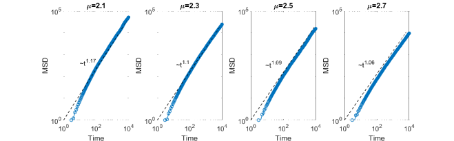
(b)

Figure 3: Average of the MSD taken from 10000 individual trajectories when we let them run for $t=10000$. (a) describes the superdiffusive regime while (b) gives the normal diffusion case.

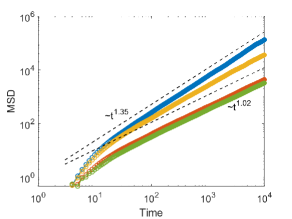
Figure 4: MSD for the non-synchronised case. The blue and yellow lines are for $\mu=1.3$ and $1.5$ respectively, and the orange and green are for the cases $\mu=2.3$ and $2.5$.

7 Conclusion and perspectives

We developed a formalism allowing to take into account how eukariotic cells move by protrusions (front of the cell) and retractions (back of the cell), keeping the simplicity of one space dimension for motion. Full generality, assuming that back and front are independent leads to a mathematical model hardly amenable to analysis, but various synchronisation levels lead to simpler models for which macroscopic effects can be observed. Among them we found normal drift-diffusion but more interestingly, instability can occur and, in the fully synchronised case, fractional diffusion characterised by long jumps. This is in accordance with experimental observations in [12] where the trajectories of metastatic cells, which move in a synchronised way, followed a power-law distribution, characteristic of a superdiffusion process.

From a modelling and analytical point of view, several questions are left open. For instance, a better understanding of the full model and of possible model reduction. Also, the introduction of more biological details, for example, in the switching direction probability (2). We could tailor this function to a specific system by knowing the internal mechanisms that leads to synchronisation in cells. Moreover, we could extend our model to several dimensions and connect it to models of cell polarisation such as [16, 17]. Finally, it would be interesting to look at the effect of the interactions with the environment and collective effects.

Appendix A Miscellaneous

(I) We compute the escape and arrival rates introduced in (63) by using the characteristic solutions (61) and (62). We start from

$$j_{\beta}(t,x)=\int_{0}^{t}p(k)\beta(t,x,k)\mathop{}\!\mathrm{d}x$$

which, by using (3) and (62), can be re-written as

$$j_{\beta}(t,x) =\int_{0}^{t}\phi(k)\beta(t-k,x+vk,0)\mathop{}\!\mathrm{d}k+{\bar{\beta}^{0}(x+vk)\phi(k)}$$

$$=\int_{0}^{t}\phi(t-s)e^{v(t-s)\partial_{x}}\beta(s,x,0)\mathop{}\!\mathrm{d}s\,+{\bar{\beta}^{0}(x+vk)\phi(k)}\ .$$ (101)

The last equality is obtained using the change of variables $k=t-s$ along with the following Taylor expansion

$$e^{v(t-s)\partial_{x}}f(x) =\sum_{m=0}^{\infty}\frac{(v(t-s)\partial_{x})^{m}}{m!}f(x)$$

$$=\sum_{m=0}^{\infty}\frac{1}{m!}(v(t-s))^{m}\partial_{x}^{m}f(x)=f(x+v(t-s))\ .$$

Analogously we can obtain (64) for $j_{\alpha}(t,x)$.

(II) Now we aim to derive the expression (88). From (84) we write, after multiplying both sides by ${\tilde{\psi}}^{+}{\tilde{\psi}}^{-}$

$${\tilde{\psi}}^{+}\,{\tilde{\psi}}^{-}\,\tilde{\rho}\,=\,{\tilde{\psi}}^{+}\,{\tilde{\phi}}^{-}\,\tilde{\bar{\beta}}\,+\,\tilde{\alpha}^{0}\,{\tilde{\psi}}^{+}\,{\tilde{\psi}}^{-}\,+\,{\tilde{\psi}}^{-}\,{\tilde{\phi}}^{+}\,\tilde{\bar{\alpha}}\,{\tilde{\psi}}^{-}\,+\,\tilde{\beta}^{0}\,{\tilde{\psi}}^{-}\,{\tilde{\psi}}^{+}\ .$$ (102)

Using the initial conditions ${\alpha}_{\varepsilon}^{0}=\varepsilon^{z}\delta(x)$ and ${\beta}^{0}(x)=0$ we obtain (88). Now, we introduce the scaling to (74) and we write

$${\tilde{\psi}}^{\pm} =-\frac{a}{1-\mu}-\frac{a^{2}\lambda_{\pm}}{(1-\mu)(2-\mu)}+a^{\alpha}\lambda_{\pm}^{\mu-1}\Gamma(-\mu+1)+\mathcal{O}(a^{3}\lambda_{\pm}^{2})\ ,$$

$${\tilde{\phi}}^{\pm} =1+\frac{a\lambda_{\pm}}{1-\mu}+a^{\mu}\lambda_{\pm}^{\mu}+O(\lambda^{\mu+1})\ .$$

Hence from here we compute

$${\tilde{\psi}}^{+}{\tilde{\phi}}^{-} =-\frac{a}{1-\mu}-\frac{a^{2}\lambda_{+}}{(1-\mu)(2-\mu)}+a^{\mu}\lambda_{+}^{\mu-1}\Gamma(-\mu+1)-\frac{a^{2}\lambda_{-}}{(1-\mu)^{2}}+\mathcal{O}(a^{\mu+1})\ ,$$

$${\tilde{\psi}}^{-}{\tilde{\phi}}^{+} =-\frac{a}{1-\mu}-\frac{a^{2}\lambda_{-}}{(1-\mu)(2-\mu)}+a^{\mu}\lambda_{-}^{\mu-1}\Gamma(-\mu+1)-\frac{a^{2}\lambda_{+}}{(1-\mu)^{2}}+\mathcal{O}(a^{\mu+1})\ ,$$

$${\tilde{\psi}}^{+}{\tilde{\psi}}^{-} =\frac{a^{2}}{(1-\mu)^{2}}-a^{\mu+1}\frac{\Gamma(\mu+1)}{1-\mu}(\lambda_{-}^{\mu-1}+\lambda^{\mu-1}_{+})+\mathcal{O}(a^{3})\ .$$

Substituting these three quantities in (102) we arrive at (89).

(III) Finally, we are going to work only with the fractional operators. Following [5, 6] we have

$$\mathds{D}_{-}^{\mu-1}\bar{\beta} =\frac{-1}{\Gamma(2-\mu)}\frac{\partial}{\partial x}\int_{x}^{\infty}\frac{\bar{\beta}(s)}{(s-x)^{\mu-1}}\mathop{}\!\mathrm{d}s=\frac{\mu-1}{\Gamma(2-\mu)}\int_{0}^{\infty}\frac{\bar{\beta}(x)-\bar{\beta}(x+s)}{s^{\mu}}\mathop{}\!\mathrm{d}s$$

$$\mathds{D}_{+}^{\mu-1}\bar{\alpha} =\frac{1}{\Gamma(2-\mu)}\frac{\partial}{\partial x}\int^{x}_{-\infty}\frac{\bar{\alpha}(s)}{(s-x)^{\mu-1}}\mathop{}\!\mathrm{d}s=\frac{\mu-1}{\Gamma(2-\mu)}\int_{0}^{\infty}\frac{\bar{\alpha}(x)-\bar{\alpha}(x-s)}{s^{\mu}}\mathop{}\!\mathrm{d}s\ .$$

The above relation is true if $\bar{\alpha},\bar{\beta}\in C^{1}(\mathds{R})$ and $\bar{\alpha},\bar{\beta}=o(|x|^{\mu-2-\epsilon})$, $x\to+\infty$ for $\epsilon>0$ (equivalence between Marchaud derivative and Riemann-Liuoville derivative).

Now we are going to use the fact that the sum $\mathds{D}_{-}^{\mu-1}f+\mathds{D}^{\mu-1}_{+}f$ gives the fractional Laplace operator in one dimension, also known as the Riesz derivative,

$$\mathds{D}_{-}^{\mu-1}\bar{\beta}+\mathds{D}_{+}^{\mu-1}\bar{\alpha} =\frac{\mu-1}{\Gamma(2-\mu)}\Bigl{(}\int_{0}^{\infty}\frac{\bar{\beta}(x)-\bar{\beta}(x+s)}{s^{\mu}}\mathop{}\!\mathrm{d}s+\int_{0}^{\infty}\frac{\bar{\alpha}(x)-\bar{\alpha}(x-s)}{s^{\mu}}\mathop{}\!\mathrm{d}s\Bigr{)}$$

$$=\frac{\mu-1}{\Gamma(2-\mu)}\Bigl{(}\int_{-\infty}^{0}\frac{\bar{\beta}(x)-\bar{\beta}(x-s)}{|s|^{\mu}}\mathop{}\!\mathrm{d}s+\int_{0}^{\infty}\frac{\bar{\alpha}(x)-\bar{\alpha}(x-s)}{s^{\mu}}\mathop{}\!\mathrm{d}s\Bigr{)}$$

$$=\frac{\mu-1}{2\Gamma(2-\mu)}\int_{-\infty}^{\infty}\frac{\bar{\beta}(x)+\bar{\alpha}(x)-\bar{\beta}(x-s)-\bar{\alpha}(x-s)}{|s|^{\mu}}\mathop{}\!\mathrm{d}s$$

$$=\frac{\mu-1}{2\Gamma(2-\mu)}\int_{-\infty}^{\infty}\frac{\rho(x)-\rho(x-s)}{|s|^{\mu}}\mathop{}\!\mathrm{d}s=\frac{\mu-1}{2\Gamma(2-\mu)}\frac{1}{c(1,\frac{\mu-1}{2})}\Bigl{(}-\frac{\mathop{}\!\mathrm{d}^{2}}{\mathop{}\!\mathrm{d}x^{2}}\Bigr{)}^{\frac{\mu-1}{2}}\rho(t,x)\ ,$$

where $c(1,\frac{\mu-1}{2})$ is a normalization constant.

References

- [1] G. Ariel, A. Rabani, S. Benisty, J. D. Partridge, R. M. Harshey, and A. Be’Er. Swarming bacteria migrate by Lévy walk. Nature Communications, 6(1):1–6, 2015.
- [2] NIST Digital Library of Mathematical Functions. http://dlmf.nist.gov/, Release 1.0.14 of 2016-12-21. F. W. J. Olver, A. B. Olde Daalhuis, D. W. Lozier, B. I. Schneider, R. F. Boisvert, C. W. Clark, B. R. Miller and B. V. Saunders, eds.
- [3] G. Estrada-Rodriguez, H. Gimperlein, and K. J. Painter. Fractional Patlak–Keller–Segel equations for chemotactic superdiffusion. SIAM Journal on Applied Mathematics, 78(2):1155–1173, 2018.
- [4] S. Fedotov, A. Tan, and A. Zubarev. Persistent random walk of cells involving anomalous effects and random death. Physical Review E, 91(4):042124, 2015.
- [5] F. Ferrari. Some nonlocal operators in the first Heisenberg group. Fractal and Fractional, 1(1):15, 2017.
- [6] F. Ferrari. Weyl and Marchaud derivatives: A forgotten history. Mathematics, 6(1):6, 2018.
- [7] S. Focardi, P. Montanaro, and E. Pecchioli. Adaptive Lévy walks in foraging fallow deer. PLoS One, 4(8):e6587, 2009.
- [8] M. Frank and T. Goudon. On a generalized Boltzmann equation for non-classical particle transport. Kinetic and Related Models, 3(3):395–407, 2010.
- [9] M. Frank and W. Sun. Fractional diffusion limits of non-classical transport equations. Kinetic and Related Models, 11(6):1503–1526, 2018.
- [10] G. M. Fricke, K. A. Letendre, M. E. Moses, and J. L. Cannon. Persistence and adaptation in immunity: T cells balance the extent and thoroughness of search. PLoS Computational Biology, 12(3):e1004818, 2016.
- [11] T. H. Harris, E. J. Banigan, D. A. Christian, C. Konradt, E. D. T. Wojno, K. Norose, E. H. Wilson, B. John, W. Weninger, A. D. Luster, et al. Generalized lévy walks and the role of chemokines in migration of effector cd8+ t cells. Nature, 486(7404):545–548, 2012.
- [12] S. Huda, B. Weigelin, K. Wolf, K. V. Tretiakov, K. Polev, G. Wilk, M. Iwasa, F. S. Emami, J. W. Narojczyk, M. Banaszak, et al. Lévy-like movement patterns of metastatic cancer cells revealed in microfabricated systems and implicated in vivo. Nature Communications, 9(1):1–11, 2018.
- [13] M. Jara, T. Komorowski, and S. Olla. Limit theorems for additive functionals of a Markov chain. The Annals of Applied Probability, 19(6):2270–2300, 2009.
- [14] E. Korobkova, T. Emonet, J. M. Vilar, T. S. Shimizu, and P. Cluzel. From molecular noise to behavioural variability in a single bacterium. Nature, 428(6982):574–578, 2004.
- [15] L. Li, S. F. Nørrelykke, and E. C. Cox. Persistent cell motion in the absence of external signals: a search strategy for eukaryotic cells. PLoS One, 3(5):e2093, 2008.
- [16] N. Loy and L. Preziosi. Kinetic models with non-local sensing determining cell polarization and speed according to independent cues. Journal of Mathematical Biology, 80(1):373–421, 2020.
- [17] N. Loy and L. Preziosi. Modelling physical limits of migration by a kinetic model with non-local sensing. Journal of Mathematical Biology, 80(6):1759–1801, 2020.
- [18] A. Mellet, S. Mischler, and C. Mouhot. Fractional diffusion limit for collisional kinetic equations. Arch. Ration. Mech. Anal., 199(2):493–525, 2011.
- [19] R. Metzler and J. Klafter. The random walk’s guide to anomalous diffusion: a fractional dynamics approach. Physics Reports, 339(1):1–77, 2000.
- [20] A. Moussa, B. Perthame, and D. Salort. Backward parabolicity, cross-diffusion and Turing instability. J. Nonlinear Sci., 29(1):139–162, 2019.
- [21] H. G. Othmer, S. R. Dunbar, and W. Alt. Models of dispersal in biological systems. Journal of Mathematical Biology, 26(3):263–298, 1988.
- [22] B. Perthame and S. Yasuda. Stiff-response-induced instability for chemotactic bacteria and flux-limited Keller-Segel equation. Nonlinearity, 31(9):4065–4089, 2018.
- [23] D. A. Raichlen, B. M. Wood, A. D. Gordon, A. Z. Mabulla, F. W. Marlowe, and H. Pontzer. Evidence of Lévy walk foraging patterns in human hunter–gatherers. Proceedings of the National Academy of Sciences, 111(2):728–733, 2014.
- [24] A. Reynolds, E. Ceccon, C. Baldauf, T. Karina Medeiros, and O. Miramontes. Lévy foraging patterns of rural humans. PLoS One, 13(6):e0199099, 2018.
- [25] A. Reynolds, G. Santini, G. Chelazzi, and S. Focardi. The weierstrassian movement patterns of snails. Royal Society open science, 4(6):160941, 2017.
- [26] A. M. Reynolds, A. D. Smith, R. Menzel, U. Greggers, D. R. Reynolds, and J. R. Riley. Displaced honey bees perform optimal scale-free search flights. Ecology, 88(8):1955–1961, 2007.
- [27] D. W. Sims, E. J. Southall, N. E. Humphries, G. C. Hays, C. J. Bradshaw, J. W. Pitchford, A. James, M. Z. Ahmed, A. S. Brierley, M. A. Hindell, et al. Scaling laws of marine predator search behaviour. Nature, 451(7182):1098–1102, 2008.
- [28] I. M. Sokolov and R. Metzler. Towards deterministic equations for Lévy walks: The fractional material derivative. Physical Review E, 67(1):010101, 2003.
- [29] G. M. Viswanathan, V. Afanasyev, S. V. Buldyrev, E. Murphy, P. Prince, and H. E. Stanley. Lévy flight search patterns of wandering albatrosses. Nature, 381(6581):413–415, 1996.
- [30] V. Zaburdaev, S. Denisov, and J. Klafter. Lévy walks. Reviews of Modern Physics, 87(2):483, 2015.