Vector-Valued Control Variates

Abstract

Control variates are variance reduction tools for Monte Carlo estimators. They can provide significant variance reduction, but usually require a large number of samples, which can be prohibitive when sampling or evaluating the integrand is computationally expensive. Furthermore, there are many scenarios where we need to compute multiple related integrals simultaneously or sequentially, which can further exacerbate computational costs. In this paper, we propose vector-valued control variates, an extension of control variates which can be used to reduce the variance of multiple Monte Carlo estimators jointly. This allows for the transfer of information across integration tasks, and hence reduces the need for a large number of samples. We focus on control variates based on kernel interpolants and our novel construction is obtained through a generalised Stein identity and the development of novel matrix-valued Stein reproducing kernels. We demonstrate our methodology on a range of problems including multifidelity modelling, Bayesian inference for dynamical systems, and model evidence computation through thermodynamic integration.

1 Introduction

A significant computational challenge in statistics and machine learning is the approximation of intractable integrals. Examples include the computation of posterior moments, the model evidence (or marginal likelihood), Bayes factors, or integrating out latent variables. This challenge has lead to the development of a wide range of Monte Carlo (MC) methods; see (Green et al., 2015) for a review. Let $f:\mathbb{R}^{d}\rightarrow\mathbb{R}$ denote some integrand of interest, and $\Pi$ some distribution with Lebesgue density $\pi$ known up to an intractable normalisation constant. The integration task we consider can be expressed as estimating

$$\textstyle\Pi[f]:=\int_{\mathbb{R}^{d}}f(x)\pi(x)\mathrm{d}x$$

using evaluations of the integrand at some points in the domain: $\{x_{i},f(x_{i})\}_{i=1}^{n}$. These evaluations are usually combined to create an estimate of $\Pi[f]$ of the form $\hat{\Pi}[f]=\frac{1}{n}\sum_{i=1}^{n}f(x_{i})$. For example, when realisations are independent and identically distributed (IID), this corresponds to a MC estimator. In that case, assuming that $f$ is square-integrable with respect to $\Pi$ (i.e. $\Pi[f^{2}]<\infty$), we can use the central limit theorem (CLT) to show that such estimators converge to $\Pi[f]$ as $n\rightarrow\infty$, and this convergence is then controlled by the asymptotic variance of the integrand $f$. Analogous results can also be obtained for Markov chain Monte Carlo (MCMC) realisations (Jones, 2004), in which case $\{x_{i}\}_{i=1}^{n}$ are realisations from a Markov Chain with invariant distribution $\Pi$, or for randomised quasi-Monte Carlo (Hickernell et al., 2005), in which case $\{x_{i}\}_{i=1}^{n}$ form some lattice or sequence filling some hypercube domain.

The main insight behind the concept of control variate (CV) is that it is instead often possible to use an estimator of $\Pi[f-g]$ for some $g:\mathbb{R}^{d}\rightarrow\mathbb{R}$. This is justified if $\Pi[g]$ is known in closed form, in which case we may use $\hat{\Pi}^{\text{CV}}[f]:=\hat{\Pi}[f-g]+\Pi[g]$. Furthermore, if $g$ is chosen appropriately, the variance of the CLT for this new estimator will be much smaller than that of the original, and a smaller number of samples will be required to approximate $\Pi[f]$ at a given level of accuracy.

Suppose now that $n=(n_{1},\ldots,n_{T})\in\mathbb{N}^{T}$ ($T\in\mathbb{N}_{+}$) is a multi-index. In this paper, we will focus on cases where we have not just one integral, but a sequence of integrands $f_{t}:\mathbb{R}^{d}\rightarrow\mathbb{R}$ and distributions $\Pi_{t}$ for which we would like to use $\{\{x_{tj},f_{t}(x_{tj})\}_{j=1}^{n_{t}}\}_{t=1}^{T}$ to estimate

$$\textstyle\Pi_{t}[f_{t}]:=\int_{\mathbb{R}^{d}}f_{t}(x)\pi_{t}(x)\mathrm{d}x\quad\text{for }t\in[T],$$ (1)

where $[T]=\{1,\ldots,T\}$. This is a common situation in practice; for example, our paper considers the case of multifidelity modelling (Peherstorfer et al., 2018) where $f_{1},\ldots,f_{T}$ may be a computationally expensive physical model $f$, and we might be interested in expectations of that model with respect to unknown parameters. Another example we will also study is when $\pi_{1},\ldots,\pi_{T}$ are closely related posterior distributions, such as in the case of power posteriors (Friel & Pettitt, 2008).

Of course, the estimation of integrals in 1 could be tackled individually, and this is in fact the most common approach. However, the main insight from this paper is that if both the integrands and distributions are related across tasks, we can improve on this by sharing computation across these tasks. We propose to construct a CV to jointly reduce the variance of estimators for these integrals and hence obtain a more accurate approximation. We will call such a function a vector-valued control variate (vv-CV). In order to encode the relationship between integration tasks, we will propose a flexible class of CV s based on interpolation in reproducing kernel Hilbert space of vector-valued functions (vv-RKHS). More precisely, we generalise existing constructions of Stein reproducing kernels to derive novel vv-RKHS s with the property that each output has mean zero.

We note that very few methods exist to tackle multiple integrals jointly. One exception is (Xi et al., 2018), which also proposes an algorithm based on vv-RKHS s. However, that work is limited to cases where the integral of the kernel is known in closed-form, which is rarely possible in practice. In contrast, our vv-CV s are applicable so long as $\pi_{t}$ is known up to an unknown constant and $\nabla_{x}\log\pi_{t}$ can be evaluated pointwise for all $t\in[T]$ (where $\nabla_{x}=(\partial/\partial x_{1},\ldots,\partial/\partial x_{d})^{\top}$). This will usually be satisfied in Bayesian statistics, and is a requirement for the implementation of most gradient-based MCMC algorithms.

The remainder is as follows. In Section 2, we review existing CV s based on Stein’s method. In Section 3, we introduce vv-CV s, then in Section 4 we show how to find an optimal vv-CV. Finally, in Section 5, we demonstrate the advantage of our approach on problems in multifidelity modelling, Bayesian inference for differential equations and model evidence computation through thermodynamic integration.

Notation

Vectors $x\in\mathbb{R}^{d}$ are column vectors, $\|x\|_{q}=(\sum_{i=1}^{d}x_{i}^{q})^{1/q}$ for $q\in\mathbb{N}$, and $\boldsymbol{1}_{d}=(1,\ldots,1)^{\top}\in\mathbb{R}^{d}$. For a multi-index $m\in\mathbb{N}^{d}$, we write $|m|=\sum_{i=1}^{d}m_{i}$ for its total degree. For a matrix $M\in\mathbb{R}^{p\times q}$, $M_{ij}$ denotes the entry in row $i$ and column $j$, $\|M\|_{F}^{2}=\sum_{i=1}^{p}\sum_{j=1}^{q}M_{ij}^{2}$ is the Frobenius squared-norm, $\text{Tr}(M)=\sum_{i=1}^{m}M_{ii}$ is the trace, and $M^{\dagger}$ is the pseudo-inverse. $I_{m}$ denotes the $m$-dimensional identity matrix, and $S^{m}_{+}$ the set of symmetric strictly positive definite matrices in $\mathbb{R}^{m\times m}$. We denote by $C^{j}$ the set of functions whose mixed partial derivatives of order at most $j$ are continuous, and given a differentiable function $g$ on $\mathbb{R}^{d_{1}}\times\mathbb{R}^{d_{2}}$, $\partial^{r}_{x}g(x,y)$ denotes its partial derivative in the $r^{th}$-coordinate of its first entry evaluated at $(x,y)$.

2 Background

We now briefly review existing constructions for Stein-based CV s for a single integration problem.

The first step consists of constructing a set of functions $\mathcal{G}$ which all integrate to a known value against $\Pi$. This can generally be challenging since $\pi$ may not be computationally tractable, e.g., involving an unknown normalisation constant. Without loss of generality, we will discuss the construction of functions which integrate to zero, but notice that we can obtain functions with mean equal to any constant $\beta\in\mathbb{R}$ by simply adding this constant $\beta$ to a zero-mean function.

Zero-Mean Functions through Stein Operators

One way of constructing zero-mean functions is to use Stein’s method (Anastasiou et al., 2023). The main ingredients of Stein’s method are a function class and an operator acting on this class. More precisely, a Stein class of $\Pi$ is a class of functions $\mathcal{U}$ associated to an operator $\mathcal{S}$, called Stein operator, such that a Stein identity holds: $\Pi[\mathcal{S}[u]]=0$ $\forall u\in\mathcal{U}$. An obvious choice for the class of zero-mean functions $\mathcal{G}$ is to consider all functions of the form $g=\mathcal{S}[u]$ for $u\in\mathcal{U}$. To ensure such $g$ has finite variance, we assume that all functions in $\mathcal{G}$ are square-integrable with respect to $\Pi$. This can be guaranteed under weak regularity conditions on $\mathcal{U}$ and $\mathcal{S}$; see Theorem 3.2. Note also that $\mathcal{S}$ depends implicitly on $\Pi$, but we only make this explicit in our notation (i. e. $\mathcal{S}_{\Pi}$) when it is helpful for clarity.

The most common choice of Stein operator is the Langevin Stein operator, which acts on differentiable vector-valued functions (vv-functions) $u:\mathbb{R}^{d}\rightarrow\mathbb{R}^{d}$:

$$\textstyle\mathcal{L}[u](x):=\nabla_{x}\cdot u(x)+u(x)\cdot\nabla_{x}\log\pi(x).$$ (2)

The advantage of $\mathcal{L}$ is that it only requires knowledge of $\Pi$ through evaluations of $\nabla_{x}\log\pi$, which does not require the normalisation constant of $\pi$. Indeed, let $\pi=\tilde{\pi}/C$ for some unknown $C\in\mathbb{R}$, then $\nabla_{x}\log\pi=\nabla_{x}\log\tilde{\pi}$. For more general Stein operators, see (Anastasiou et al., 2023).

Parametric Spaces

$\mathcal{G}$ is usually chosen to be a parametric space and we will hence write it $\mathcal{G}_{\Theta}$, where $\Theta$ denotes the space of parameter values. Most existing CV s can be obtained by taking $g_{\theta}=\mathcal{S}[u_{\theta}]$ for some $u_{\theta}\in\mathcal{U}_{\Theta}$ where $\mathcal{U}_{\Theta}$ is another parametric class. However, note that there might not be a unique $u_{\theta}$ leading to $g_{\theta}$. For the remainder of the paper, $\theta$ will hence be a parameter indexing $g_{\theta}$ directly as opposed to an element of the Stein class. Examples of parametric CV s are the polynomial-based CV s of (Mira et al., 2013) (see also (Assaraf & Caffarel, 1999; Papamarkou et al., 2014; Oates et al., 2016)), in which case the Stein class is parametrised directly by coefficients of a polynomial. Using a space of neural networks has also been studied in (Wan et al., 2019; Si et al., 2021). This later choice can be advantageous due to the flexibility of this function class, but is much more challenging to implement because selecting a CV becomes a non-convex problem.

Another example are kernel interpolants, which will be the main focus of our paper. This class is nonparametric, but it is often convenient to fix the dataset size and parametrise it. Let $\mathcal{H}_{k}$ denote a reproducing kernel Hilbert space (RKHS) with kernel $k:\mathbb{R}^{d}\times\mathbb{R}^{d}\rightarrow\mathbb{R}$ (Berlinet & Thomas-Agnan, 2011), so that $k$ is symmetric ($k(x,y)=k(y,x)$ $\forall x,y\in\mathbb{R}^{d}$) and positive semi-definite ($\forall m\in\mathbb{N}_{+}$, $\sum_{i,j=1}^{m}c_{i}c_{j}k(x_{i},x_{j})\geq 0$ $\forall c_{1},\ldots,c_{m}\in\mathbb{R}$ and $\forall x_{1},\ldots,x_{m}\in\mathbb{R}^{d}$). The kernel could be a squared-exponential kernel $k(x,y)=\exp(-\|x-y\|_{2}^{2}/2l^{2})$ with lengthscale $l>0$, or a polynomial kernel $k(x,y)=(x^{\top}y+c)^{l}$ where $c\in\mathbb{R}$ and $l\in\mathbb{N}$ is the degree of the polynomial. Oates et al. (2017) noticed that the image of $\mathcal{U}=\mathcal{H}_{k}^{d}:=\mathcal{H}_{k}\times\ldots\times\mathcal{H}_{k}$ under $\mathcal{L}$ is a RKHS with kernel

$$\textstyle k_{0}(x,y) \textstyle:=\nabla_{x}\cdot\nabla_{y}k(x,y)+\nabla_{x}\log\pi(x)\cdot\nabla_{y}k(x,y)$$

$$\textstyle\quad+\nabla_{y}\log\pi(y)\cdot\nabla_{x}k(x,y)$$

$$\textstyle\quad+(\nabla_{x}\log\pi(x)\cdot\nabla_{y}\log\pi(y))k(x,y),$$ (3)

see also Thm 2.6 Barp et al. (2022b) for a more general result. Given $m$ observations, it is known that the optimal interpolant in $\mathcal{H}_{k_{0}}$ is of the form $g_{\theta}(x)=\sum_{i=1}^{m}\theta_{i}k_{0}(x,x_{i})$ where $\theta_{i}\in\mathbb{R}$ for all $i\in[m]$. This therefore provides a natural parametrisation for practical implementation. Oates et al. (2017) called this class of CV s control functionals (CF); see also (Briol et al., 2017; Oates et al., 2019; South et al., 2022a) for more details.

Selecting a CV

In order to select a CV, we will pick the “best” element from $\mathcal{G}_{\Theta}$, where “best” will refer to minimising MC variance:

$$\textstyle J(\theta)=\text{Var}_{\Pi}[f-g_{\theta}]:=\Pi[(f-g_{\theta}-\Pi[f])^{2}],$$ (4)

Following the framework of empirical risk minimisation, this can be approximated with $\{x_{j},f(x_{j})\}_{j=1}^{m}$ as follows:

$$\textstyle J_{m}(\theta,\beta) \textstyle=\frac{1}{m}\sum_{j=1}^{m}(f(x_{j})-g_{\theta}(x_{j})-\beta)^{2}+\lambda\|g_{\theta}\|^{2},$$

where $\beta\in\mathbb{R}$ is an additional parameter which tends to $\Pi[f]$ as $m\rightarrow\infty$ and $\lambda\rightarrow 0$. Here, $\lambda\geq 0$ is a regularisation parameter and $\|g_{\theta}\|$ can be any suitable norm. For example, $\|g_{\theta}\|=\|\theta\|_{2}$ or $\|g_{\theta}\|=\|g_{\theta}\|_{\mathcal{H}_{k}}$ for some kernel $k$. Assuming that $\Theta\subseteq\mathbb{R}^{p}$, this objective can then be minimised by the solution to a linear system when $\theta\mapsto g_{\theta}$ is linear and $\theta\mapsto\|g_{\theta}\|^{2}$ is quadratic. In more general cases, it can be minimised using stochastic optimisation (Si et al., 2021). In that case, we initialise $\theta^{(0)}$ and $\beta^{(0)}$, then iteratively take gradient steps with minibatches of size $\tilde{m}\ll m$.

There are two particular perspectives which motivate the objective in (4). Firstly, it can be interpreted as a least-squares objective for the function $f-\Pi[f]$ (Leluc et al., 2021). Secondly, by noticing that for any square-integrable function $h$ and MC estimator with $n$ samples we have $\text{Var}_{\Pi}[\hat{\Pi}^{\text{MC}}[h]]=\text{Var}_{\Pi}[h]/n$, we can notice that $J(\theta)$ fully determines the CLT variance of a MC estimator of $\Pi[f-g_{\theta}]$, which makes it particularly well suited for these estimators. This latter viewpoint has also motivated alternative objectives based on the variance of the randomised quasi-Monte Carlo or MCMC CLT; see e.g. Hickernell et al. (2005); Oates & Girolami (2016); Dellaportas & Kontoyiannis (2012); Mijatovic & Vogrinc (2018). The MCMC case is briefly discussed in Section A.1, but the remainder of the paper will focus on the objective in (4) for simplicity.

The CV Estimator

Recall that a CV estimator takes the form $\hat{\Pi}^{\text{CV}}[f]:=\hat{\Pi}[f-g]+\Pi[g]$ for some CV $g$. Once a function $g_{\hat{\theta}}$ has been selected through the procedure in the previous subsection, the only part missing is therefore an estimator for $\Pi[f-g_{\hat{\theta}}]$. We present two possible approaches below. A first option is to create an estimator based on the remainder of the data $\{x_{i},f(x_{i})\}_{i=m+1}^{m+n}$:

$$\textstyle\hat{\Pi}[f-g_{\hat{\theta}}]=\frac{1}{n}\sum_{i=m+1}^{m+n}(f(x_{i})-g_{\hat{\theta}}(x_{i})).$$

This estimator is unbiased whenever $\hat{\Pi}[f-g_{\hat{\theta}}]$ is unbiased. This is the case when using a MC estimator, but not when using a MCMC estimator. The question of how to select $m$ is of practical importance for the quality of the estimator. When $m$ is small, most of the function evaluations are used for the MC estimator, whereas when $m$ is large, most of the evaluations are used to construct the CV.

Due to the difficulty of choosing $m$, a second option is to use all of the data for selecting $g_{\hat{\theta}}$ (i.e. $n=0$). More precisely, denoting by $(\hat{\theta},\hat{\beta})$ the minimiser of $J_{m}(\theta,\beta)$, we could use $\hat{\Pi}[f-g_{\hat{\theta}}]=\hat{\beta}$. This estimator will be biased, but will also be more accurate than the first estimator if the least-squares problem can be solved at a fast rate than the MC CLT.

3 Methodology

We will now extend existing CV s to the case where multiple related integration problems are tackled jointly. This will be done through a multi-task learning approach (Micchelli & Pontil, 2005; Evgeniou et al., 2005), where each integral corresponds to a task and the relationship between tasks will be modelled explicitly. This will allow us to share information across integration tasks, and hence improve accuracy when the number of integrand evaluations is limited.

3.1 Vector-Valued Functions using Stein’s Method

For the remainder of this paper, we consider integrands corresponding to the outputs of a vector-valued function $f:\mathbb{R}^{d}\rightarrow\mathbb{R}^{T}$ so that $f(x)=(f_{1}(x),\ldots,f_{T}(x))^{\top}$. Our objective is to approximate $\Pi[f]=(\Pi_{1}[f_{1}],\ldots,\Pi_{T}[f_{T}])^{\top}$, and we shall assume that $f_{t}$ is square-integrable with respect to $\Pi_{t}$ $\forall t\in[T]$. Formally, $\Pi$ is known as a vector probability distribution. To approximate $\Pi[f]$, we will construct a class of zero-mean vv-functions through Stein’s method. This can be done by considering a Stein class $\mathcal{U}$ whose image $\mathcal{G}$ under the Stein operator $\mathcal{S}^{\text{vv}}:\mathcal{U}\rightarrow\mathcal{G}$ is a class of $\mathbb{R}^{T}$-valued functions on $\mathbb{R}^{d}$. We will need a generalised form of Stein identity for vv-functions:

$$\textstyle\Pi_{t}[g_{t}]=\Pi_{t}[(\mathcal{S}^{\text{vv}}[u])_{t}]=0,~{}~{}\forall u\in\mathcal{U}\text{ and }\forall t\in[T].$$ (5)

In other words, each output of the vv-function should integrate to zero against the corresponding probability distribution. Of course, the ordering of the sequence of integrands and distributions matters here, as we do not guarantee that $\Pi_{t}[g_{t^{\prime}}]=0$ for $t\neq t^{\prime}$. The property above can be obtained by constructing an operator $\mathcal{S}^{\text{vv}}$ through a sequence of Stein operators $\mathcal{S}^{\text{sv}}_{\Pi_{t}}$ for $t\in[T]$ whose images are scalar-valued functions integrating to zero under $\Pi_{t}$. These can then be applied in an element-wise fashion as follows

$$\textstyle g=\mathcal{S}^{\text{vv}}[u]=(\mathcal{S}^{\text{sv}}_{\Pi_{1}}[u_{1}],\ldots,\mathcal{S}^{\text{sv}}_{\Pi_{T}}[u_{T}])^{\top}.$$ (6)

Once again, $\mathcal{G}$ can be parametrised and we will denote it $\mathcal{G}_{\Theta}$. We can then use an objective based on the variances $f-g_{\theta}$ to select an optimal element:

$$\textstyle J^{\text{vv}}(\theta)=\|\text{Var}_{\Pi}[f-g_{\theta}]\| \textstyle=\|\Pi[(f-g_{\theta}-\Pi[f])^{2}]\|,$$ (7)

where $g_{\theta}\in\mathcal{G}_{\Theta}$. In the above $\text{Var}_{\Pi}$ should be thought of as applying $\text{Var}_{\Pi_{t}}$, the variance under $\Pi_{t}$, to the $t^{\text{th}}$ element of the vv-function. The norm could be any norm on $\mathbb{R}^{T}$, but we will usually make use of the $1$-norm so as to interpret this objective as the sum of variances on each integrand. For this objective to make sense, we require $(g_{\theta})_{t}$ to be squared-integrable with respect to $\Pi_{t}$ $\forall t\in[T]$. Similarly to the $T=1$ case, we are focusing on a least-squares objective, which directly controls the variance of MC estimators, but this could be adapted to other estimators as previously discussed.

Let $m=(m_{1},\ldots,m_{T})\in\mathbb{N}_{+}^{T}$. Once again, the objective can be approximated via MC estimates based on the dataset $\mathcal{D}=\{\{x_{1j},f_{1}(x_{1j})\}_{j=1}^{m_{1}},\ldots,\{x_{Tj},f_{T}(x_{Tj})\}_{j=1}^{m_{T}}\}$ following the framework of empirical risk minimisation. For example, when the norm above is a $1$-norm, the objective is simply the sum of individual variances:

$$\textstyle L^{\text{vv}}_{m}(\theta,\beta):=J^{\text{vv}}_{m}(\theta,\beta)+\lambda\|g_{\theta}\|^{2}$$ (8)

$$\textstyle=\sum_{t=1}^{T}\frac{1}{m_{t}}\sum_{j=1}^{m_{t}}(f_{t}(x_{tj})-(g_{\theta}(x_{tj}))_{t}-\beta_{t})^{2}+\lambda\|g_{\theta}\|^{2},$$

where $\lambda\geq 0$ and now $\beta=(\beta_{1},\ldots,\beta_{T})\in\mathbb{R}^{T}$. Once again, the second term is used to regularise $J^{\text{vv}}_{m}$, but the norm acts on vv-functions. For $\mathcal{U}$, we could take a class of polynomials, kernels or neural networks, but will usually require flexible classes of vv-functions in order to encode relationships between tasks. Assuming that each $\Pi_{t}$ has a $C^{1}$ and strictly positive density $\pi_{t}$ with respect to the Lebesgue measure, we will also be able to use the Langevin Stein operators $\mathcal{L}$, which only require access to the score functions for each distribution $\Pi_{1},\ldots,\Pi_{T}$. For this purpose, we now define $l:\mathbb{R}^{d}\rightarrow\mathbb{R}^{T\times d}$ to be the matrix-valued function with entries $l_{ij}(x)=\partial^{j}\log\pi_{i}(x)$.

3.2 Kernel-based Vector-Valued CV s

The main choice of Stein class $\mathcal{U}$ studied in this paper is vv-RKHS s (Carmeli et al., 2006, 2010; Álvarez et al., 2012). This choice is particularly convenient as it allows us to build on the rich literature in statistical learning theory which considers kernels encoding relationships between tasks. A main contribution of this section will be the design of novel Stein reproducing kernels specifically for numerical integration, a task not commonly tackled in statistical learning theory.

A vv-RKHS $\mathcal{H}_{K}$ is a Hilbert space of functions mapping from $\mathbb{R}^{d}$ to $\mathbb{R}^{T}$ with an associated matrix-valued reproducing kernel (mv-kernel) $K:\mathbb{R}^{d}\times\mathbb{R}^{d}\rightarrow\mathbb{R}^{T\times T}$ which is symmetric ($K(x,y)=K(y,x)^{\top}$ $\forall x,y\in\mathbb{R}^{d}$) and positive semi-definite ($\forall m\in\mathbb{N}_{+}$, $\sum_{i,j=1}^{m}c_{i}^{\top}K(x_{i},x_{j})c_{j}\geq 0$ for all $c_{1},\ldots,c_{m}\in\mathbb{R}^{T}$ and $x_{1},\ldots,x_{m}\in\mathbb{R}^{d}$). Any vv-RKHS satisfies a reproducing property, so that $\forall f\in\mathcal{H}_{K}$, $f(x)^{\top}c=\langle f,K(\cdot,x)c\rangle_{\mathcal{H}_{K}}$ and $K(\cdot,x)c\in\mathcal{H}_{K}$ $\forall x\in\mathbb{R}^{d}$ and $\forall c\in\mathbb{R}^{T}$. The reproducing kernels discussed in Section 2 are a special case which can be recovered when $T=1$. We say that $K$ is $C^{r,r}(\mathbb{R}^{d}\times\mathbb{R}^{d})$ provided that $\partial^{\alpha}_{x}\partial^{\alpha}_{y}K(x,y)$ is continuous for all multi-indices $\alpha=(\alpha_{1},\ldots,\alpha_{d})$ with $\alpha_{1}+\cdots+\alpha_{d}\leq r$, and that $K$ is bounded with bounded derivatives if there exists $C\geq 0$ for which $\|\partial_{x}^{\alpha}\partial_{y}^{\alpha}K(x,y)\|_{F}\leq C$ for all $x,y\in\mathbb{R}^{d}$ and multi-indices $\alpha$ with $\alpha_{1}+\cdots+\alpha_{d}\leq 1$.

To construct vv-CV s, a natural approach is to construct a mv-kernel $K_{0}$ using another mv-kernel $K$ and an operator $\mathcal{S}^{\text{vv}}$. Then, assuming we have access to such a $K_{0}$ and to data $\mathcal{D}$, a natural generalisation of the scalar valued case is:

$$\textstyle g_{\theta}(x)=\sum_{t=1}^{T}\sum_{j=1}^{m_{t}}K_{0}(x,x_{tj})\theta_{tj},$$ (9)

where $\theta_{tj}\in\mathbb{R}^{T}$, for all $t\in[T],j\in[m_{t}]$. The remainder of this section will hence focus on how to obtain $K_{0}$. Our construction is based on the CF s of (Oates et al., 2017, 2019), which use a scalar-valued kernel $k_{0}$ obtained through a tensor product structure $\mathcal{U}=\mathcal{H}_{k}^{d}$. The initial motivation for introducing vv-functions in this setting was that $\mathcal{L}$ requires inputs which are vv-functions which can be thought of as introducing a dummy dimension for convenience, and is in no way related to the multitask setting in this paper. We now illustrate the natural extension of $k_{0}$ to a mv-kernel.

Theorem 3.1.

Consider $\mathcal{H}_{K}$ which is a vv-RKHS with mv-kernel $K:\mathbb{R}^{d}\times\mathbb{R}^{d}\rightarrow\mathbb{R}^{T\times T}$, and suppose that $K\in C^{1,1}(\mathbb{R}^{d}\times\mathbb{R}^{d})$. Furthermore, assuming $u=(u_{1},\ldots,u_{T})\in\mathcal{H}_{K}$, let $\mathcal{S}^{\text{vv}}[u]=(\mathcal{L}_{\Pi_{1}}[u_{1}],\ldots,\mathcal{L}_{\Pi_{T}}[u_{T}])^{\top}$. Then, the image of $\mathcal{H}_{K}^{d}=\mathcal{H}_{K}\times\ldots\times\mathcal{H}_{K}$ under $\mathcal{S}^{\text{vv}}$ is a vv-RKHS with kernel $K_{0}:\mathbb{R}^{d}\times\mathbb{R}^{d}\rightarrow\mathbb{R}^{T\times T}$ with:

$$\textstyle(K_{0}(x,y))_{tt^{\prime}}=\sum_{r=1}^{d}\partial^{r}_{x}\partial^{r}_{y}K(x,y)_{tt^{\prime}}+l_{t^{\prime}r}(y)\partial^{r}_{x}K(x,y)_{tt^{\prime}}$$

$$\textstyle\qquad\qquad+l_{tr}(x)\partial_{y}^{r}K(x,y)_{tt^{\prime}}+l_{tr}(x)l_{t^{\prime}r}(y)K(x,y)_{tt^{\prime}},$$

The proof is in Section B.1. Notice that $(K_{0}(x,y))_{tt^{\prime}}$ depends only on the score function of $\Pi_{t}$ and $\Pi_{t^{\prime}}$, and so we (once again) do not require knowledge of normalisation constants. However, in order to evaluate $K_{0}(x,y)$ for some $x,y\in\mathbb{R}^{d}$, we will require pointwise evaluation of $\nabla_{x}\log\pi_{t}(x)$ and $\nabla_{y}\log\pi_{t}(y)$ for all $t\in[T]$. Finally, another interesting point is that $(K_{0}(x,y))_{tt^{\prime}}$ is a scalar-valued kernel when $t=t^{\prime}$, but this is not the case for $t\neq t^{\prime}$ since it is not symmetric in that case.

To use elements of this RKHS as vv-CV s, we will require that the least-squares objective in 7 is well-defined. This can be guaranteed when the elements of the RKHS are square-integrable, and the theorem below, proved in Section B.2, provides sufficient conditions for this to hold.

Theorem 3.2.

Suppose that $K$ is bounded with bounded derivatives, and $\Pi_{t}[\|\nabla_{x}\log\pi_{t}\|_{2}^{2}]<\infty$ for all $t\in[T]$. Then, for any $g\in\mathcal{H}_{K_{0}}$, $g_{t}$ is square-integrable with respect to $\Pi_{t}$ for all $t\in[T]$.

Now the mv-kernel in Theorem 3.1 takes a very general form as it has minimal requirements on $K$ or $\Pi_{1},\ldots,\Pi_{T}$. This is convenient as it can be applied in a wide range of settings, but this generality comes at the cost of computational complexity. We will now study several special cases which will often be sufficient for applications.

Special Case I: Separable kernel $K$

For simplicity, the literature on multi-task learning often focuses on the case of separable kernels. We say a mv-kernel $K$ is separable if it can be written as $K(x,y)=Bk(x,y)$, where $k$ is a scalar valued kernel and $B\in S^{T}_{+}$. The advantage of this formulation is that it decouples the model for individual outputs (as given by $k$) from the model of their relationship, as given by the components of the matrix $B$, which can be thought of as a covariance matrix for tasks. As we will see in Section 4, this can be particularly advantageous for selecting the hyperparameters of vv-CV s. Using such a kernel $K$, the kernel $K_{0}$ in Theorem 3.1 becomes:

$$\textstyle(K_{0}(x,y))_{tt^{\prime}} \textstyle=B_{tt^{\prime}}\sum_{r=1}^{d}\partial^{r}_{x}\partial^{r}_{y}k(x,y)+l_{t^{\prime}r}(y)\partial^{r}_{x}k(x,y)$$

$$\textstyle\quad+l_{tr}(x)\partial_{y}^{r}k(x,y)+l_{tr}(x)l_{t^{\prime}r}(y)k(x,y),$$

for $\forall t,t^{\prime}\in[T]$. This expression is interesting because it reduces the choice of $K$ to the choice of a matrix $B$ and a kernel $k$, and this matrix $B$ has a natural interpretation in that $B_{tt^{\prime}}$ denotes the covariance between $f_{t}$ and $f_{t}^{\prime}$. See Section E.1 for illustrations of such $K_{0}$.

Special Case II: Separable kernel $K$ with one target distribution

A further simplification of the kernel is possible when $K$ is separable and all distributions are the same: $\Pi_{1}=\cdots=\Pi_{T}\equiv\Pi$. In this case $K_{0}$ itself becomes a separable kernel of the form: $(K_{0}(x,y))_{tt^{\prime}}=B_{tt^{\prime}}k_{0}(x,y)$ $\forall t,t^{\prime}\in[T]$, where $k_{0}$ is given in Section 2. The scalar case can then be recovered by taking $T=1$ and $B=1$.

Selecting a Base Kernel and Alternative Constructions

The base kernel $K$ needs to be chosen by the user. As for the scalar case, we expect that the performance of our approach will depend on whether the smoothness of $K_{0}$ closely matches the smoothness of the integrand $f$, and the smoothness of $K$ should therefore be chosen accordingly. We also suggest selecting the hyperparameters of $K$ through either cross validation or through maximisation of the log-marginal likelihood of a zero-mean multi-output Gaussian process with kernel $K_{0}$; see Section D.2 for details. Furthermore, see Appendix C for alternative constructions, including vv-CV s derived from the second-order matrix-valued Stein kernels and vv-CV s based on other parametric spaces such as polynomials and neural networks.

4 Selecting a Vector-Valued CV

We will now derive both a closed-form expression for the optimal parameters of these kernel-based vv-CV s and a stochastic optimisation scheme to approximate it.

Closed-form Solutions

We start with a theorem which provides a result akin to the RKHS representer theorem, but which focuses specifically on the function which minimises the objective in 8. This theorem shows that there exists a unique parameter minimising the variance objective.

Theorem 4.1.

Let $\mathcal{D}=\{\{x_{1j},f_{1}(x_{1j})\}_{j=1}^{m_{1}},\ldots,\{x_{Tj},f_{T}(x_{Tj})\}_{j=1}^{m_{T}}\}$. The function which minimises the objective in 8 where $\|g_{\theta}\|:=\|g_{\theta}\|_{\mathcal{H}_{K_{0}}}$ and $\beta\in\mathbb{R}^{T}$ is of the form:

$$\textstyle g_{\theta}(x)=\sum_{t=1}^{T}\sum_{j=1}^{m_{t}}\theta_{tj}^{\top}K_{0}(x,x_{tj}),\theta_{tj}\in\mathbb{R}^{T}$$

with optimal parameter $\theta^{*}$ given by the solution of this convex linear system of equations:

$$\textstyle\sum_{t^{\prime}}\sum_{j^{\prime}}\Big{(}\sum_{t}\frac{1}{m_{t}}\sum_{j}K_{0}(x_{t^{\prime\prime}j^{\prime\prime}},x_{tj})_{\cdot t}K_{0}(x_{tj},x_{t^{\prime}j^{\prime}})_{t\cdot}$$

$$\textstyle\qquad\qquad+\lambda K_{0}(x_{t^{\prime\prime}j^{\prime\prime}},x_{t^{\prime}j^{\prime}})\Big{)}\theta_{t^{\prime}j^{\prime}}^{*}$$

$$\textstyle=\sum_{t}\frac{1}{m_{t}}\sum_{j}K_{0}(x_{t^{\prime\prime}j^{\prime\prime}},x_{tj})_{\cdot t}(f_{t}(x_{tj})-\beta_{t}),$$

$\forall t^{\prime\prime}\in[T],j^{\prime\prime}\in[m_{T}]$.

Furthermore, if $K_{0}$ is strictly positive definite and the points $x_{tj}$ are distinct, then the system is strictly convex and $\theta^{*}$ is unique.

See Section B.3 for the proof. Theorem 4.1 assumes that $\beta$ is known and fixed, which may not be the case in practice. However, given a fixed $g_{\theta}$ the objective 8 is a quadratic in $\beta$ with the optimal value $\beta^{*}_{t}=\frac{1}{m_{t}}\sum_{j=1}^{m_{t}}f_{t}(x_{tj})-(g_{\theta}(x_{tj}))_{t}$. This naturally leads to the use of block coordinate descent approaches which iterate between optimising $\beta$ and $\theta$. This could be either directly implemented using the closed-form solutions, or through the use of numerical optimisers such as the stochastic optimisation approaches we will now present. The next paragraph highlights how this can be implemented for special case I and II. We remark that the use of stochastic optimisation tools will be essential in most applications due to the size of the linear systems leading exact solutions to being intractable in practice.

Algorithm 1 Block-coordinate descent for vv-CV s with unknown task relationship

  Input: $\mathcal{D},\tilde{m},L,\lambda,\beta^{(0)},\theta^{(0)}$ and $B^{(0)}$

  for iteration $l=1$ to $L$ do

     Select a mini-batch $\mathcal{D}_{\tilde{m}}$ of size $\tilde{m}=(\tilde{m}_{1},\ldots,\tilde{m}_{T})^{\top}$

     $\big{(}\theta^{(l)},\beta^{(l)}\big{)}\leftarrow\textsc{Update}_{\theta,\beta}(\theta^{(l-1)},\beta^{(l-1)},B^{(l-1)};\mathcal{D}_{\tilde{m}}\big{)}$

     $B^{(l)}\leftarrow\textsc{Update}_{B}\big{(}\theta^{(l)},\beta^{(l)},B^{(l-1)};\mathcal{D}_{\tilde{m}}\big{)}$.

  end for

  Return: $\theta^{(L)}$, $\beta^{(L)}$ and $B^{(L)}$

Unknown Task Relationship

We now extend our approach to account for simultaneously estimating $\beta$, $\theta$, but also the matrix $B$. In this setting, we will use the same objective as in 8, but penalised by the norm of $B$:

$$\textstyle\bar{L}^{\text{vv}}_{m}(\theta,\beta,B)=J^{\text{vv}}_{m}(\theta,\beta,B)+\lambda\|g_{\theta}\|^{2}+\|B\|^{2},$$ (10)

We now use $J^{\text{vv}}_{m}(\theta,\beta,B)$ to denote $J^{\text{vv}}_{m}(\theta,\beta)$ in order to emphasise the dependence on $B$. A second regularisation parameter is unnecessary as this would be equivalent to rescaling $k$. The objective in 10 is a natural extension to 8 and can be straightforwardly minimised through stochastic optimisation; see Algorithm 1. To ensure $B$ is strictly positive definite, we can take $B=LL^{\top}$, where $L$ is a lower triangular matrix with diagonal elements forced to be greater than zero via an exponential transformation. The pseudo-code in Algorithm 1 presents this abstractly as a function Update. This is because different choices of vv-CV s might benefit from different updates. For example, pre-conditioners for the gradients could be used when readily available, or when these can be estimated from data. In Section 5, we will exclusively be using the Adam optimiser (Kingma & Ba, 2015), a first-order method with estimates of lower-order moments. Additionally, we study the convex case when $B$ is known and only $\beta$ and $\theta$ are required to be estimated in Section A.2.

Computational Complexity

Although vv-CV s can be beneficial from an accuracy viewpoint, they also incur a significant computational cost. Whether they should be used will therefore depend on the computational budget available. In particular, when evaluations of $f$ or $\nabla\log\pi$ are expensive, the higher cost of using vv-CV s may be negligible. Table 1 provides the computational complexity of all approaches considered in the paper. We emphasise the impact of $T$, the number of tasks. In the case of existing kernel-based CV s, the dependence is $\mathcal{O}(T)$. In contrast, the computational cost of vv-CV s is between $\mathcal{O}(T^{4})$ and $\mathcal{O}(T^{6})$. Table 1 also highlights the difference in computational complexity between obtaining closed form solutions of $\theta$ and $\beta$ by solving the linear system of equations in Theorem 4.1, and using the stochastic-optimisation approaches in Section A.2 and Section 4. Here, the difference is mainly in terms of powers of $T$, $m_{t}$ and $\tilde{m}_{t}$. As we can see the exact solutions usually come with an $\mathcal{O}(m_{t}^{3})$ cost, whereas the stochastic optimisation approach is associated with a $\mathcal{O}(m_{t}\tilde{m}_{t}L)$ cost. In this case, whenever $\tilde{m}_{t}L$ is small relative to $m_{t}$, this will lead to computational gains.

In all applications considered, both $m_{t}$ and $T$ were small so the overall cost is controlled. However, this computational complexity can be further significantly reduced in special cases. When using a kernel corresponding to a finite-dimensional RKHS (e.g. a polynomial kernel), the scaling becomes linear in $m_{t}$, but is $\mathcal{O}(q^{3})$ instead of $\mathcal{O}(m_{t}^{3})$, where $q\ll m_{t}$ is the dimensionality of the RKHS. Alternatively, for certain choices of point sets and kernels, it is possible to reduce the computational complexity to $\mathcal{O}(m_{t}\log m_{t})$ instead of $\mathcal{O}(m_{t}^{3})$ by using scalable kernel methods such as fast Fourier features or inducing points. When the integrands are evaluated at the same set of points and the separable kernel is used, the computational cost in $T$ also becomes $\mathcal{O}(T^{2})$ instead of $\mathcal{O}(T^{6})$, once again significantly reducing the computational complexity.

Table 1: Computational complexity of kernel-based CV s and vv-CV s as a function of $d,m,\tilde{m},L$ and $T$. We assume that $m_{t}$ is the same $\forall t\in[T]$ up to additive or multiplicative constants (and similarly for all $\tilde{m}_{t}$ with $t\in[T]$). The cost of stochastic optimisation algorithms is assumed to only scale with the cost of stochastic estimates of the gradient of $J^{\text{vv}}$.

Method	CV	vv-CV
Exact solution	$\mathcal{O}((dm_{t}^{2}+m_{t}^{3})T)$	$\mathcal{O}(dm_{t}^{2}T^{4}+m_{t}^{3}T^{6})$
Stochastic optim.	$\mathcal{O}(d\tilde{m}_{t}m_{t}LT)$	$\mathcal{O}(d\tilde{m}_{t}m_{t}LT^{4})$

5 Experimental Results

We now illustrate our method on a range of problems including multi-fidelity models, computation of the model evidence for dynamical systems through thermodynamic integration and Bayesian inference for the abundance of preys using a Lotka-Volterra system. See Appendix E for additional experiments including illustrations of matrix-valued Stein kernels $K_{0}$ in Section E.1 and a synthetic example when the Stein kernel matches the smoothness of integrands in Section E.2. Since we are interested in gains obtained from the CV s, we fix $n=0$ which means we are using all the data to construct vv-CV s. The code to reproduce our results is available at: https://github.com/jz-fun/Vector-valued-Control-Variates-Code.

5.1 Multidelity Modelling in the Physical Sciences

Many problems in the engineering and physical sciences can be tackled with multiple models of a single system of interest. These models are often associated with varying computational costs and levels of accuracy, and their combination to solve a task is usually called multi-fidelity modelling; see (Peherstorfer et al., 2018) for a review. We will consider a high-fidelity model $f_{H}$ and a low-fidelity model $f_{L}$, and will attempt to estimate the integral of $f_{H}$ with our vv-CV s and using function evaluations from both the high- and low-fidelity models. For clarity, we will now denote the function $f=(f_{L},f_{H})$ and the vector-probability distribution $\Pi=(\Pi_{L},\Pi_{H})$. We note that this is a special case of the problem considered in our paper since we use evaluations of multiple functions but are only interested in $\Pi_{H}[f_{H}]$ (whereas $\Pi_{L}[f_{L}]$ is not of interest).

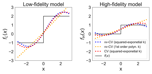
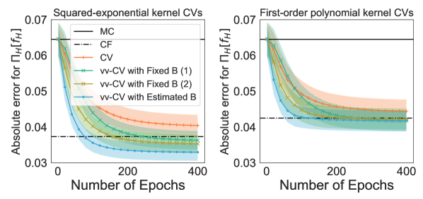
Figure 1: Numerical integration of univariate discontinuous multifidelity model. Upper: fitted CVs for both functions. Lower Left: performance of CV s based on a squared-exponential kernel for the high-fidelity function as a number of epochs of the optimisation algorithm. The lines provide the mean over $100$ repetitions of the experiment, whereas the shaded areas provide one standard deviation above and below the mean. Lower Right: same experiment for a polynomial kernel for the high-fidelity function.

Univariate Step Function

The first example considered is a toy problem from the multi-fidelity literature (Xi et al., 2018). The low-fidelity function is $f_{\text{L}}(x)=2~{}\text{if}~{}x\geq 0$ and $-1~{}\text{otherwise}$. The high-fidelity function is $f_{\text{H}}(x)=1~{}\text{if}~{}x\geq 0$ and $0~{}\text{otherwise}$. In this example, $K_{0}$ is smoother than $f_{1}$ and $f_{2}$, which are both discontinuous. The integral is over the real line and taken against $\Pi=\mathcal{N}(0,1)$, and we fix the sample sizes to $m=(m_{\text{L}},m_{\text{H}})=(40,40)$.

Results with a squared-exponential and 1${}^{\text{st}}$ order polynomial kernel $k$ can be found in Figure 1. The upper plots clearly show that the approximations are not of very high-quality, but the lower plots show that all CV s can still lead to an order of two gain in accuracy over MC methods. We also observe that vv-CV s can lead to further gains over existing CV s by leveraging evaluations of $f_{L}$. For both kernels, we provide three different versions of the vv-CV s with separable structure to highlight the impact of the matrix $B$. The first two cases use Algorithm 2 with a fix value of $B$. In the first instance, $B_{11}=B_{22}=0.1,B_{12}=B_{21}=0.01$, whereas in the second instance $B_{11}=B_{22}=0.5,B_{12}=B_{21}=0.01$. The third case is based on estimating $B$ through Algorithm 1. Clearly, $B$ can have a significant impact on the performance of the vv-CV, and estimating a good value from data can provide further gains. The choice of $k$ is also significant: all CV s based on the squared-exponential kernel significantly outperform the CV s based on a 1${}^{\text{st}}$ order polynomial kernel. It is also found that even when the model is mis-specified, the proposed method still perform better than standard scalar-valued CV s.

Modelling of Waterflow through a Borehole

A more complex example often used to assess multifidelity methods is the following model of water flow passing through a borehole (Xiong et al., 2013; Kandasamy et al., 2016; Park et al., 2017). Both $f_{L}$ and $f_{H}$ have $d=8$ inputs representing a range of parameters influencing the geometry and hydraulic conductivity of the borehole, as well as transmissivity of the aquifer. Prior distributions have been elicited from scientists over input parameters to account for uncertainties about their exact value. See Section E.4 for the details of each input and the multi-fidelity models. One quantity of interest here is the expected water flow under these distributions, and we hence have $\Pi_{L}=\Pi_{H}$.

Table 2: Expected values of the flow of water through a borehole. The numbers provided give the mean absolute integration error for $100$ repetition of the task of estimating $\Pi_{H}[f_{H}]$, and the numbers in brackets provide the sample standard deviation. To provide the absolute error, the true value ($72.8904$) is estimated by a MC estimator with $5\times 10^{5}$ samples.

$m$	vv-CV- Est. B	vv-CV-Fix. B	CF	MC
$10$	3.72 (0.27)	1.94 (0.15)	2.24 (0.16)	6.42 (0.44)
$20$	1.29 (0.10)	1.35 (0.10)	1.96 (0.10)	4.31 (0.31)
$50$	1.04 (0.06)	1.77 (0.12)	1.76 (0.07)	2.63 (0.17)
$100$	1.07 (0.06)	1.65 (0.14)	1.71 (0.05)	1.83 (0.15)
$150$	0.85 (0.05)	1.30 (0.09)	1.67 (0.04)	1.42 (0.10)

Results of our simulation study are presented in Table 2. We compare a standard MC estimator with a kernel-based CV fitted with a closed form solution (denoted CF) and two kernel-based vv-CV s corresponding to special case II in Section 3. The first with $B_{11}=B_{22}=5\times 10^{-4}$ and $B_{12}=B_{21}=5\times 10^{-5}$, and the second with $B$ estimated using Algorithm 1. The kernel used is a tensor product of squared-exponential kernels with a separate lengthscale for each dimension. Clearly, vv-CV s significantly outperform MC in the large majority of cases, and estimating $B$ can lead to significant gains over using a fixed $B$. The worst performance for vv-CV s with estimated $B$ is when values of $m$ are the lowest. This is because $m$ is not large enough to learn a good $B$. See Section E.4 for further details.

5.2 Model Evidence for Dynamical Systems

We now consider Bayesian inference for non-linear differential equations such as dynamical systems, which can be particularly challenging due to the need to compute the model evidence. This is usually a computationally expensive task since sampling from the posterior repeatedly requires the use of a numerical solver for differential equations which needs to be used at a fine resolution.

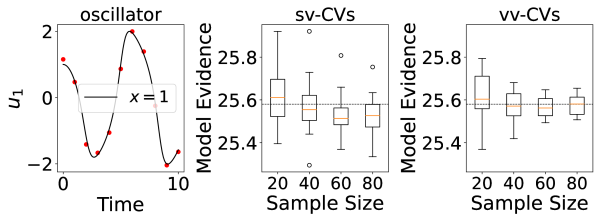
Figure 2: Model evidence computation through thermodynamic integration. Left: Illustration of the van der Poll oscillator model (black line) and corresponding observations (red dots). Center: Estimates of the model evidence as a function of the number of posterior samples for kernel-based CV s. The box-plots were created by repeating the experiment $20$ times and the black line gives an estimate of the truth obtained from (Oates et al., 2017) ($25.58$). Right: Same experiment but with kernel-based vv-CV s.

In (Calderhead & Girolami, 2009), the authors propose to use thermodynamic integration (TI) (Friel & Pettitt, 2008) to tackle this problem, and (Oates et al., 2016, 2017) later showed that CV s can lead to significant gains in accuracy in this context. TI introduces a path from the prior $p(x)$ to the posterior $p(x|y)$, where $y$ and $x$ represent the observations and the unknown parameters respectively. This is accomplished by the power posterior $p(x|y,t)\propto p(y|x)^{t}p(x)$, where $t\in[0,1]$ is called the inverse temperature. When $t=0$, $p(x|y,t)=p(x)$, whereas when $t=1$, $p(x|y,t)=p(x|y)$. The standard TI formula for the model evidence has a simple form which can be approximated using second-order quadrature over a discretised temperature ladder $0=t_{1}\leq\cdots\leq t_{w}=1$ (Friel et al., 2014). It takes the following form

$$\textstyle\log p(y)=\int_{0}^{1}\left[\int_{\mathcal{X}}\log p(y|x)p(x|y,t)d\theta\right]dt$$

$$\textstyle\qquad\approx\sum_{i=1}^{w}\frac{t_{i+1}-t_{i}}{2}(\mu_{i+1}+\mu_{i})-\frac{(t_{i+1}-t_{i})^{2}}{12}(v_{i+1}-v_{i}),$$

where $\mu_{i}$ is the mean and $v_{i}$ the variance of the integrand $f(x):=\log p(y|x)$ with respect to $\pi_{i}(x):=p(x|y,t_{i})$. To estimate $\{\mu_{i},v_{i}\}_{i=1}^{w}$, we need to sample from all power posteriors on the ladder, then use a MCMC estimator which can be enhanced through CV s. This gives $T=2w$ integrals which are related: $w$ integrals to compute means and $w$ integrals to compute variances, each against different power posteriors. As we will see, this structure will allow vv-CV s to provide significant gains in accuracy.

Our experiments will focus on the van der Poll oscillator, which is an oscillator $u:\mathbb{R}_{+}\times\mathcal{X}\rightarrow\mathbb{R}$ (where $x\in\mathbb{R}$) given by the solution of $d^{2}u/ds^{2}-x(1-u^{2})du/ds+u=0$, where $s$ represents the time index. For this experiment, we will follow the exact setup of (Oates et al., 2017) and transform the equation into a system of first order equations: $\nicefrac{{du_{1}}}{{ds}}=u_{2},\nicefrac{{du_{2}}}{{ds}}=x(1-u_{1}^{2})u_{2}-u_{1}$, which can be tackled with ODE solvers. Our data will consist of noisy observation of $u_{1}$ (the first component of that system) given by $y(s)=\mathcal{N}(u_{1}(s;x),\sigma^{2})$ with $\sigma=0.1$ at each point $s\in\{0,1,\ldots,10\}$; see the left-most plot of Figure 2 for an illustration. We will take a ladder of size $w=31$ with $t_{i}=((i-1)/30)^{5}$ for $i\in\{1,\ldots,31\}$. This gives a total of $T=62$ integrals will need to be computed simultaneously, which is likely to be too computationally expensive for vv-CV s in their full generality. As a result, we chose $B$ to be a block diagonal matrix which puts integrands in groups of $4$ means or $4$ variances (except one group of 3 for mean and variance). To sample from the power-posteriors, we use population MC with the manifold Metropolis-adjusted Langevin algorithm (Girolami & Calderhead, 2011). Due to the high computational cost of using ODE solvers, our number of samples will be limited to less than $100$ per integrand and this number will be the same for each integration task.

Our results are presented in Figure 2. The kernel parameters were taken to be identical to those in (Oates et al., 2017). As observed in the centre plot, kernel-based CV s provide relatively accurate estimates of the model evidence. As the sample size increases, we notice less variability in these estimates, but the central $50\%$ of the runs are contained in an interval which excludes the true value. In comparison, the right-most plot shows that kernel-based vv-CV s can provide significant further reduction in variance. The distribution of estimates is also much more concentrated and centered around the true value.

5.3 Bayesian Inference of Lotka-Volterra System

We now consider another model: the Lotka-Volterra system (Lotka, 1925; Volterra, 1926; Lotka, 1927) of ordinary differential equations. This system is given by: $\nicefrac{{dv_{1}(s)}}{{ds}}=\alpha v_{1}(s)-\beta v_{1}(s)v_{2}(s),\nicefrac{{dv_{2}(s)}}{{ds}}=\delta v_{1}(s)v_{2}(s)-\gamma v_{2}(s)$. Here, $s\in[0,S]$ for some $S\in\mathbb{R}_{+}$ denotes the time, and $v_{1}(s)$ and $v_{2}(s)$ are the numbers of preys and predators, respectively. The system has initial conditions $v_{1}(0)$ and $v_{2}(0)$. We have access to noisy observations of $v=(v_{1},v_{2})$ at points $s_{1},\ldots,s_{m}\in[0,S]$ denoted $y_{1j},y_{2j}$ and which are both observed with log-normal noise with standard deviation $\sigma_{y_{1}}$ and $\sigma_{y_{2}}$ respectively for all $j\in\{1,\ldots,m\}$, given some unknown parameter value $x^{*}=(\alpha^{*},\beta^{*},\delta^{*},\gamma^{*},v_{1}(0)^{*},v_{2}(0)^{*},\sigma_{y_{1}}^{*},\sigma_{y_{2}}^{*})^{\top}$. In practice, we reparameterise $x$ such that the model parameters are defined in $\mathbb{R}^{8}$; see Section E.6 for details. Given these observations, we can construct a posterior $\Pi$ on the value of $x^{*}$. We will then be interested in computing posterior expectations of $v_{1}$ at a set of time points $s^{\prime}_{1},\ldots,s^{\prime}_{T}$, and hence have $T$ integrands of the form $f_{t}(x)=v_{1}(s_{t}^{\prime};x)$ where $x$ highlights the dependence on the parameter $x$. CV s were previously considered for individual tasks in this context by Si et al. (2021). However, these $T$ integrands are related when $s^{\prime}_{1},\ldots,s^{\prime}_{T}$ are close to each other.

We use the dataset of snowshoe hares (preys) and Canadian lynxes (predators) from Hewitt (1921), and implement Bayesian inference on model parameters $x$ by using no-U-turn sampler (NUTS) in Stan (Carpenter et al., 2017). For sv-CVs, we estimate each individual $\Pi[f_{t}]$ separately; while for vv-CV s, we estimate a collection these tasks $\Pi[f]:=(\Pi[f_{1}],\ldots,\Pi[f_{T}])^{\top}$ jointly. See Section E.6 for experimental details. In Table 3, we compare kernel vv-CV s (special case II) with standard MCMC estimators and CF estimators. We consider two cases of vv-CV s: the first is the case when $B$ is with $B_{tt}=5\times 10^{-4}$ for all $t$ and $B_{tt^{\prime}}=5\times 10^{-5}$ for $\forall t\neq t^{\prime}$, and the second with $B$ estimated using Algorithm 2. The kernel used is a tensor product of squared-exponential kernels with a separate lengthscale for each dimension. We increase the number of tasks from $T=2$ to $T=10$. Once again, vv-CV s significantly outperforms MCMC, especially for large $T$, and estimating $B$ provides further gains over using a fixed $B$.

Table 3: Posterior Expected Abundance of Preys. The numbers provided give the sum of the mean absolute integration error for $10$ repetition of each task. To provide the absolute error, the true values of the associated expectations are estimated by MCMC estimators with $8\times 10^{5}$ posterior samples.

$T$	$m$	vv-CV- Est. B	vv-CV-Fix. B	CF	MCMC
$2$	$500$	0.462	0.404	0.666	0.568
$5$	$500$	0.393	0.419	0.521	0.987
$10$	$500$	0.938	1.031	2.540	2.663

6 Conclusion

This paper considered variance reduction techniques that share information across related integration problems. The proposed solution, vector-valued control variates, was shown to lead to significant variance reduction for problems in multi-fidelity modelling and Bayesian computation. Our approach is, to the best of our knowledge, the first algorithm able to perform multi-task learning for numerical integration by using only evaluation of the score functions of the corresponding target distributions. It is also the first algorithm which can simultaneously learn the relationship between integrands and provide estimates of the corresponding integrals without the requirement of a tractable kernel mean as in (Xi et al., 2018).

On an algorithmic level, further work will be needed to make the method more computationally practical and efficient. One particular line of research which could be considered is how special cases of our matrix-valued Stein kernels in Theorem 3.1 can be selected to reduce the computational cost whilst still producing a rich class of vv-CV s. Since a preprint version of this paper appeared online, it has been shown that approaches based on meta-learning could be competitive for very large $T$; see Sun et al. (2023).

On a theoretical level, we could also look at the question of when transferring information across tasks will lead to sufficient gains in accuracy to warrant the additional computational cost. In addition, it could be of interest to understand the negative transfer problems which can arise when the integrands are not in RKHS $\mathcal{H}_{K_{0}}$ or when the sample size is too small to estimate $B$ well.

Appendix

We now complement the main text with additional details. Firstly, we provide additional methodology in Appendix A, including alternative objectives based on the variance of MCMC, stochastic optimisation algorithm for vv-CV s when the task relationship $B$ is known (under special case I and II) and the calculation of the computational complexity that is presented in Table 1. Secondly, in Appendix B, we provide the proofs of all the theoretical results in the main text. Then, in Appendix C, we present alternative constructions of vv-CV s. These constructions include a more general form of kernel-based vv-CV s as well as some polynomial-based CV s. Finally, in Appendix D and Appendix E, we provide additional details on our implementation of vv-CV s and provide additional numerical experiments.

Appendix A Additional Methodology

In this first appendix, we will present additional methodology for Section 3. We briefly discuss an alternative objective based on the variance of the MCMC case in Section A.1. The selection of vv-CV s under special case I and II when $B$ is known and the corresponding algorithm is presented in Section A.2.

A.1 Alternative Objectives based on the Variance of MCMC

We present an alternative objective based on the variance of MCMC here, which is given by the following remark.

Remark 1.

Given $\{X_{i}\}_{i=1}^{\infty}$ an ergodic Markov chain with invariant distribution $\Pi$, the variance of the MCMC CLT is proportional to

$$\textstyle J(\theta)+2\sum_{i=1}^{\infty}\text{Cov}_{\Pi}[f(X_{1})-g_{\theta}(X_{1}),f(X_{i})-g_{\theta}(X_{i})]$$

where the second term accounts for the correlation in the Markov chain. Given some realisation of the Markov chain $\{x_{j}\}_{j=1}^{m}$ and the corresponding evaluations $\{f(x_{j})\}_{j=1}^{m}$, this can be approximated as:

$$\textstyle J_{m}(\theta,\beta)+2\sum_{s=1}^{m-1}\frac{1}{m}\sum_{i=1}^{m-s}(f(x_{i})-g_{\theta}(x_{i})-\hat{\Pi}^{\text{MC}}[f-g_{\theta}])(f(x_{i+s}-g_{\theta}(x_{i+s})-\hat{\Pi}^{\text{MC}}[f-g_{\theta}])).$$

A.2 Stochastic Optimisation with a Known Task Relationship

In this section, we discuss the selection of vv-CV s under special case I and II when $B$ is known and give the corresponding algorithm in Algorithm 2.

In this case, we will assume that $B\in S_{+}^{T}$ is known. The proposed algorithm is a stochastic optimisation algorithm which we run for $L$ time steps; pseudo-code is provided in Algorithm 2. We propose to initialise the algorithm at $\theta^{(0)}=(0,\ldots,0)\in\mathbb{R}^{p}$, since this is equivalent to having $g_{\theta}(x)=0$ (i.e. having no CV) for both the kernel- and polynomial-based vv-CV s. We also suggest initialising the parameter $\beta\in\mathbb{R}^{T}$ with any estimate of $\Pi[f]$. This is a natural initialisation since we expect $\beta_{t}$ to equal $\Pi[f_{t}]$ for all $t\in[T]$ when $m_{1},\ldots,m_{T}\rightarrow\infty$. For example, when the data consists of IID realisations from $\Pi_{1},\ldots,\Pi_{T}$, a natural initialisation point is $\beta^{(0)}=(\hat{\Pi}^{\text{MC}}_{1}[f_{1}],\ldots,\hat{\Pi}^{\text{MC}}_{T}[f_{T}])^{\top}$.

For each iteration, we take mini-batches of size $\tilde{m}\in\mathbb{N}^{T}$ where $|\tilde{m}|\leq|m|$. Note here that $\tilde{m}=(\tilde{m}_{1},\ldots,\tilde{m}_{T})^{\top}$ is a multi-index giving the size of the mini-batch for each of the $T$ datasets. This formulation allows for the use of different datasets across integrands, but also different mini-batch sizes for each task (which may be useful if the datasets are of different size for each integrand). An epoch consists of having gone through all data points for all $T$ tasks, and we randomly shuffle the indices for mini-batches after each epoch. As default, we propose to take $\tilde{m}_{t}\propto m_{t}/(\sum_{t=1}^{T}m_{t})$ for all $t\in[T]$. This choice guarantees that the number of samples for each integrand in the mini-batches is proportional to the proportion of samples for that integrand in the full dataset.

Once a mini-batch has been selected, we update our current estimate of the parameters $\theta$ and $\beta$ using steps based on the gradient of our loss function: $\nabla_{(\theta,\beta)}L^{\text{vv}}_{\tilde{m}}(\theta,\beta)$. The pseudo-code in Algorithm 2 presents this abstractly as a function $\textsc{Update}_{\theta,\beta}(\theta,\beta,B;\mathcal{D})$, which takes in the current estimates of the parameters, the value of $B$ and the dataset (or minibatch) used for the update; this is because different choices of vv-CV s might benefit from different updates. For example, pre-conditioners for the gradients could be used when readily available, or when these can be estimated from data. In Section 5, we will exclusively be using the Adam optimiser (Kingma & Ba, 2015), a first order method with estimates of lower-order moments.

For the penalisation term, it would be natural to take the RKHS norm $\|g_{\theta}\|=\|g_{\theta}\|_{\mathcal{H}_{K_{0}}}$ since this would lead to the objective used in Theorem 4.1. However, this can be impractical from a computational viewpoint since this norm depends on kernel evaluations for all of the training points. For this reason, we follow the recommendation of (Si et al., 2021) and use instead the Euclidean norm: $\|g_{\theta}\|=\|\theta\|_{2}$. This still leads to a convex objective since the objective remains quadratic in $\theta$.

Algorithm 2 is a natural approach to minimising our objective since our kernel-based vv-CV s are linear in $\theta$ and $L^{\text{vv}}_{m}$ is convex in $(\theta,\beta)$. Many stochastic optimisation methods, such as stochastic gradient descent, will hence converge to a global minimum under regularity conditions (Bottou et al., 2018). However, note that Algorithm 2 naturally applies to other vv-CV s whether linear or not.

Algorithm 2 Stochastic optimisation for vv-CV s with known task relationship

  Input: $\mathcal{D}$, $\tilde{m}$, $L$, $\lambda$, $\beta^{(0)}$ and $\theta^{(0)}$.

  for iterations $l$ from $1$ to $L$ do

     Select a mini-batch $\mathcal{D}_{\tilde{m}}$ of size $\tilde{m}$

     $\big{(}\theta^{(l)},\beta^{(l)}\big{)}\leftarrow\textsc{Update}_{\theta,\beta}(\theta^{(l-1)},\beta^{(l-1)},B;\mathcal{D}_{\tilde{m}}\big{)}$

  end for

  Return: $\theta^{(L)}$, $\beta^{(L)}$

A.3 Calculation of Computational Complexity

In this section, we derive the computational complexity reported in Table 1. Suppose we have $m_{t}$ samples for each of $T$ tasks and similarly for all $\tilde{m}_{t}$ with $t\in[T]$.

Computational cost of CV:

• Exact solution: For each task, we need to compute $k_{0}(\cdot,\cdot)$ for all pairs, which results in a cost of $\mathcal{O}(dm_{t}^{2})$ per task. To compute the exact solution of kernel-based control variates, it takes $\mathcal{O}(m_{t}^{3})$ per task. So, in total, the computational cost of the exact solution of CV is $\mathcal{O}((dm_{t}^{2}+m_{t}^{3})T)$.

• Stochastic optimisation: To use stochastic optimisation, suppose we use $L$ epochs. At each iteration of one epoch, we need to compute $k_{0}(\cdot,\cdot)$ for $\tilde{m}_{t}m_{t}$ pairs, which costs $\mathcal{O}(d\tilde{m}_{t}m_{t})$. We need to do this for all $L$ iterations. This results in $\mathcal{O}(d\tilde{m}_{t}m_{t}L)$ per task. Hence, in total, the computational cost of stochastic optimisation of CV is $\mathcal{O}(d\tilde{m}_{t}m_{t}LT)$ for all $T$ tasks.

Computational cost of vv-CV:

• Exact solution: There are $m_{t}T$ samples (i.e. $m_{t}^{2}T^{2}$ pairs) in total and we are using mv-Stein kernels. Thus, the computational cost of computing $K_{0}(\cdot,\cdot)$ is $\mathcal{O}(d(m_{t}T)^{2}T^{2})=\mathcal{O}(dm_{t}^{2}T^{4})$. To compute the exact solution of vv-CV, we can re-arrange the Gram tensor of all samples into a matrix of size $m_{t}T^{2}\times m_{t}T^{2}$. Hence, the computational cost of computing the exact solution of vv-CV is $\mathcal{O}((m_{t}T^{2})^{3})=\mathcal{O}(m_{t}^{3}T^{6})$. Thus, in total, the computational cost of computing the exact solution of vv-CV is $\mathcal{O}(dm_{t}^{2}T^{4}+m_{t}^{3}T^{6})$.

• Stochastic optimisation: At each iteration, one mini-batch of the stochastic optimisation of vv-CV has $\tilde{m_{t}}T$ samples. We need to compute $K_{0}(\cdot,\cdot)$ for these samples with all $m_{t}T$ samples. This leads to a cost of $\mathcal{O}(\tilde{m}_{t}Tm_{t}TdT^{2})=\mathcal{O}(d\tilde{m}_{t}m_{t}T^{4})$ per iteration. Note that we need to do this for all $L$ iterations. So, in total, the computational cost of stochastic optimisation of vv-CV is $\mathcal{O}(d\tilde{m}_{t}m_{t}LT^{4})$.

Appendix B Proofs of the Main Theoretical Results

In this second appendix, we recall the proofs of the theoretical results in the main text. The derivation of the mv-kernel $K_{0}$ from Theorem 3.1 can be found in Section B.1. The proof that kernel-based vv-CV s are square-integrable (Theorem 3.2) is in Section B.2. Finally, the proof of the existence of the optimal parameters as the solution to a linear system (Theorem 4.1) is given in Section B.3.

B.1 Proof of Theorem 3.1

Proof.

We will show $K_{0}$ is a kernel and derive its matrix components by constructing an appropriate feature map. The first order Stein operator maps matrix-valued functions $u=(u_{1},u_{2}\ldots,u_{T}):\mathbb{R}^{d}\to\mathbb{R}^{d\times T}$ to the vv-function $\mathcal{S}^{\text{vv}}[u]:\mathbb{R}^{d}\to\mathbb{R}^{T}$ given by

$$\textstyle\mathcal{S}^{\text{vv}}[u] \textstyle=\left(\mathcal{L}_{\Pi_{1}}\left[u_{1}\right],\ldots,\mathcal{L}_{\Pi_{T}}\left[u_{T}\right]\right)^{\top}$$

$$\textstyle\text{ where }\quad\mathcal{L}_{\Pi_{t}}[u_{t}](x) \textstyle=\nabla_{x}\cdot u_{t}(x)+\nabla_{x}\log\pi_{t}(x)\cdot u_{t}(x)\quad\forall t\in[T].$$

Since $K\in C^{1,1}(\mathbb{R}^{d}\times\mathbb{R}^{d})$, we can use Corollary 4.36 of (Steinwart & Christmann, 2008) to conclude that $\mathcal{H}_{K}$ is a vector-valued RKHS of continuously differentiable functions from $\mathbb{R}^{d}$ to $\mathbb{R}^{T}$, hence the tensor product $\mathcal{H}_{K}^{d}$ consists of suitable functions $u\in\mathcal{H}_{K}^{d}$, with components $u^{i}=(u_{1}^{i},\ldots,u_{T}^{i})\in\mathcal{H}_{K}$ for $i\in[d]$. Now since the RKHS consists of differentiable functions, we have by Lemma C.8 in Barp et al. (2022b):

$$\textstyle\left<\partial^{j}_{x}K(\cdot,x)e_{t},u^{i}\right>_{\mathcal{H}_{K}}=e_{t}\cdot\partial^{j}u^{i}(x)=\partial^{j}u_{t}^{i}(x)\equiv\frac{\partial u_{t}^{i}}{\partial x^{j}}(x)\quad\forall t\in[T]$$

where $e_{t}\in\mathbb{R}^{T}$ is a vector of zeros with value $1$ in the $t^{\text{th}}$ component. Then, writing $K^{e_{t}}_{x}\equiv K(\cdot,x)e_{t}$,

$$\textstyle\mathcal{S}^{\text{vv}}[u](x) \textstyle=\sum_{t=1}^{T}\sum_{r=1}^{d}(\partial^{r}_{x}u_{t}^{r}(x)+\partial^{r}_{x}\log\pi_{t}\,u_{t}^{r}(x))e_{t}$$

$$\textstyle=\sum_{t=1}^{T}\sum_{r=1}^{d}\left<\partial^{r}_{x}K_{x}^{e_{t}}+l_{tr}(x)K_{x}^{e_{t}},u^{r}\right>_{\mathcal{H}_{K}}e_{t}$$

$$\textstyle=\sum_{t=1}^{T}\left<\partial^{\bullet}_{x}K_{x}^{e_{t}}+l_{t\bullet}(x)K_{x}^{e_{t}},u\right>_{\mathcal{H}_{K}^{d}}e_{t},$$

where $l_{tr}(x)=\partial^{r}_{x}\log\pi_{t}(x)$, and $\partial_{x}^{\bullet}K_{x}^{e_{t}}$ and $l_{t\bullet}(x)$ denote respectively the tuples $(\partial_{x}^{1}K_{x}^{e_{t}},\ldots,\partial_{x}^{d}K_{x}^{e_{t}})\in\mathcal{H}_{K}^{d}$ and $(l_{t1}(x),\ldots,l_{td}(x))\in\mathbb{R}^{d}$.

We have thus obtained a feature map, i.e., a map $\gamma:\mathbb{R}^{d}\to\mathcal{B}(\mathcal{H}_{K}^{d},\mathbb{R}^{T})$, where $\mathcal{B}(\mathcal{H}_{K}^{d},\mathbb{R}^{T})$ denotes the space of bounded linear maps from $\mathcal{H}_{K}^{d}$ to $\mathbb{R}^{T}$, via the relation

$$\textstyle\gamma(x)[u]=\mathcal{S}^{\text{vv}}[u](x),$$

with adjoint $\gamma(x)^{*}=\sum_{t=1}^{T}(\partial^{\bullet}_{x}K_{x}^{e_{t}}+l_{t\bullet}(x)K_{x}^{e_{t}})e_{t}$. Recall the adjoint map $\gamma(y)^{*}\in\mathcal{B}(\mathbb{R}^{T},\mathcal{H}_{K}^{d})$ to $\gamma(y)$, is defined for any $a\in\mathbb{R}^{T},u\in\mathcal{H}_{K}^{d}$ by the relation

$$\textstyle\left<\gamma(y)^{*}[a],u\right>_{\mathcal{H}_{K}^{d}}=\gamma(y)[u]\cdot a.$$

In particular, by Proposition 1 of Carmeli et al. (2010) we have that

$$\textstyle K_{0}(x,y)\equiv\gamma(x)\circ\gamma(y)^{*}\in\mathbb{R}^{T\times T}$$

will then be the kernel associated to the “feature operator” (that is, a surjective partial isometry whose image is $\mathcal{H}_{K_{0}}$) $\mathcal{S}^{\text{vv}}:\mathcal{H}_{K}^{d}\to\mathcal{H}_{K_{0}}$. Subbing in the expressions for the feature map and its adjoint derived above, and using the equalities

$$\textstyle\left<\partial^{s}_{x}K(\cdot,x)e_{t},\partial_{y}^{r}K(\cdot,y)e_{t^{\prime}}\right>_{\mathcal{H}_{K}}=e_{t}\cdot\partial^{s}_{x}\partial_{y}^{r}K(x,y)e_{t^{\prime}}=(\partial^{s}_{x}\partial_{y}^{r}K(x,y))_{tt^{\prime}}\qquad\forall t,t^{\prime}\in[T]$$

$$\textstyle\text{and }\qquad\left<\partial^{ss}_{x}K(\cdot,x)e_{t},\partial_{y}^{r}K(\cdot,y)e_{t^{\prime}}\right>_{\mathcal{H}_{K}}=(\partial^{ss}_{x}\partial_{y}^{r}K(x,y))_{tt^{\prime}}\qquad\forall t,t^{\prime}\in[T],$$

which hold for any differentiable matrix-valued kernel (Barp et al., 2022b), we obtain the following expression for the components of $K_{0}$

$$\textstyle(K_{0}(x,y))_{tt^{\prime}} \textstyle=\sum_{r=1}^{d}(\partial^{r}_{x}\partial^{r}_{y}K(x,y))_{tt^{\prime}}+l_{t^{\prime}r}(y)(\partial^{r}_{x}K(x,y))_{tt^{\prime}}$$

$$\textstyle\qquad+l_{tr}(x)\partial_{y}^{r}(K(x,y))_{tt^{\prime}}+l_{tr}(x)l_{t^{\prime}r}(y)(K(x,y))_{tt^{\prime}}.$$

In particular for separable kernels (i.e. $K(x,y)=Bk(x,y)$) we have

$$\textstyle(K_{0}(x,y))_{tt^{\prime}}=B_{tt^{\prime}}\sum_{r=1}^{d}\partial^{r}_{x}\partial^{r}_{y}k(x,y)+l_{t^{\prime}r}(y)\partial^{r}_{x}k(x,y)+l_{tr}(x)\partial_{y}^{r}k(x,y)+l_{tr}(x)l_{t^{\prime}r}(y)k(x,y).$$

∎

B.2 Proof of Theorem 3.2

Proof.

Recall that if a scalar kernel $k$ satisfies $\int_{\mathbb{R}^{d}}k(x,x)\mathrm{d}\mu(x)<\infty$, then its RKHS consists of square $\mu$-integrable functions (for any finite measure $\mu$) (Steinwart & Christmann, 2008, Theorem 4.26).

If $g\in\mathcal{H}_{K_{0}}$ then $g_{t}$ belongs to the RKHS with scalar-valued kernel (this follows from (Carmeli et al., 2010, Prop. 1), using as feature operator the dot product with respect to $e_{t}$, where $e_{t}$ is defined in Section B.1)

$$\textstyle(K_{0}(x,y))_{tt} \textstyle=\sum_{r=1}^{d}(\partial^{r}_{x}\partial^{r}_{y}K(x,y))_{tt}+l_{tr}(y)\partial^{r}_{x}(K(x,y))_{tt}$$

$$\textstyle\quad+l_{tr}(x)\partial_{y}^{r}(K(x,y))_{tt}+l_{tr}(x)l_{tr}(y)(K(x,y))_{tt}\qquad\forall t\in[T].$$

In particular since $K$ is bounded with bounded derivatives, and

$$\textstyle\Pi_{t}\left[|l_{tr}|\right]+\Pi_{t}\left[|l_{tr}|^{2}\right]\leq\sqrt{\Pi_{t}\left[|l_{tr}|^{2}\right]}+\Pi_{t}\left[|l_{tr}|^{2}\right]\qquad\forall t\in[T],r\in[d]$$

then $\int_{\mathbb{R}^{d}}(K_{0}(x,x))_{tt}\mathrm{d}\Pi_{t}(x)<\infty$ if $\|\nabla_{x}\log\pi_{t}(x)\|_{2}$ is square integrable with respect to $\Pi_{t}$, and the result follows. ∎

B.3 Proof of Theorem 4.1

Proof.

We want to find

$$\textstyle\operatorname*{arg\,min}_{g\in\mathcal{H}_{K_{0}}}L^{\text{vv}}_{m}(g,\beta)$$

$$\textstyle\text{ where }\qquad L^{\text{vv}}_{m}(g,\beta) \textstyle:=\sum_{t=1}^{T}\frac{1}{m_{t}}\sum_{j=1}^{m_{t}}(f_{t}(x_{tj})-g_{t}(x_{tj})-\beta_{t})^{2}+\lambda\|g\|^{2}_{\mathcal{H}_{K_{0}}}.$$

Note that the objective is the same as that in 8, with the only difference being that the first input is now a function as opposed to the parameter value parameterising this function. We will abuse notation by using the same mathematical expression for both objectives.

By Ciliberto et al. (2015, Section 2.1), any solution of the minimization problem has the form $\hat{g}(\cdot)\equiv\sum_{t^{\prime}=1}^{T}\sum_{j^{\prime}=1}^{m_{t^{\prime}}}K_{0}(\cdot\,,x_{t^{\prime}j^{\prime}})\theta_{t^{\prime}j^{\prime}}$. Subbing this solution into $L^{\text{vv}}_{m}(g,\beta)$ yields

$$\textstyle L^{\text{vv}}_{m}(\hat{g},\beta) \textstyle=\sum_{t=1}^{T}\frac{1}{m_{t}}\sum_{j=1}^{m_{t}}(f_{t}(x_{tj})-(\sum_{t^{\prime}=1}^{T}\sum_{j^{\prime}=1}^{m_{t^{\prime}}}K_{0}(x_{tj},x_{t^{\prime}j^{\prime}})_{t}\theta_{t^{\prime}j^{\prime}}-\beta_{t})^{2}$$

$$\textstyle\qquad+\lambda\sum_{t^{\prime},t^{\prime\prime}=1}^{T}\sum_{j^{\prime}=1}^{m_{t^{\prime}}}\sum_{j^{\prime\prime}=1}^{m_{t^{\prime\prime}}}\theta_{t^{\prime}j^{\prime}}^{T}K_{0}(x_{t^{\prime}j^{\prime}},x_{t^{\prime\prime}j^{\prime\prime}})\theta_{t^{\prime\prime}j^{\prime\prime}}$$

$$\textstyle=\lambda\sum_{t^{\prime},t^{\prime\prime}=1}^{T}\sum_{j^{\prime}=1}^{m_{t^{\prime}}}\sum_{j^{\prime\prime}=1}^{m_{t^{\prime\prime}}}\theta_{t^{\prime}j^{\prime}}^{T}K_{0}(x_{t^{\prime}j^{\prime}},x_{t^{\prime\prime}j^{\prime\prime}})\theta_{t^{\prime\prime}j^{\prime\prime}}$$

$$\textstyle\qquad+\sum_{t=1}^{T}\frac{1}{m_{t}}\sum_{j=1}^{m_{t}}\Big{(}y_{tj}^{2}+(\sum_{t^{\prime}=1}^{T}\sum_{j^{\prime}=1}^{m_{t^{\prime}}}K_{0}(x_{tj},x_{t^{\prime}j^{\prime}})_{t}\theta_{t^{\prime}j^{\prime}})^{2}$$

$$\textstyle\qquad\qquad\qquad\qquad\qquad\qquad-2\sum_{t^{\prime}=1}^{T}\sum_{j^{\prime}=1}^{m_{t^{\prime}}}y_{tj}K_{0}(x_{tj},x_{t^{\prime}j^{\prime}})_{t}\theta_{t^{\prime}j^{\prime}}\Big{)},$$

where $y_{tj}\equiv f_{t}(x_{tj})-\beta_{t}$. The problem thus becomes a minimization problem over the coefficients $\theta$,

$$\textstyle\operatorname*{arg\,min}_{\theta\in\mathbb{R}^{|\mathcal{D}|}}\lambda \textstyle\sum_{t^{\prime},t^{\prime\prime}=1}^{T}\sum_{j^{\prime}=1}^{m_{t^{\prime}}}\sum_{j^{\prime\prime}=1}^{m_{t^{\prime\prime}}}\theta_{t^{\prime}j^{\prime}}^{T}K_{0}(x_{t^{\prime}j^{\prime}},x_{t^{\prime\prime}j^{\prime\prime}})\theta_{t^{\prime\prime}j^{\prime\prime}}$$

$$\textstyle-2\sum_{t,t^{\prime}=1}^{T}\frac{1}{m_{t}}\sum_{j=1}^{m_{t}}\sum_{j^{\prime}=1}^{m_{t^{\prime}}}\theta_{t^{\prime}j^{\prime}}^{T}K_{0}(x_{t^{\prime}j^{\prime}},x_{tj})_{\cdot t}y_{tj}+\sum_{t=1}^{T}\frac{1}{m_{t}}\sum_{j=1}^{m_{t}}y_{tj}^{2}$$

$$\textstyle+\sum_{t,t^{\prime},t^{\prime\prime}=1}^{T}\sum_{j=1}^{m_{t}}\sum_{j^{\prime}=1}^{m_{t^{\prime}}}\sum_{j^{\prime\prime}=1}^{m_{t^{\prime\prime}}}\theta_{t^{\prime}j^{\prime}}^{T}K_{0}(x_{t^{\prime}j^{\prime}},x_{tj})_{\cdot t}\frac{1}{m_{t}}K_{0}(x_{tj},x_{t^{\prime\prime}j^{\prime\prime}})_{t\cdot}\theta_{t^{\prime\prime}j^{\prime\prime}}.$$

Since the quadratic terms are positive definite, the resulting objective is a convex function of $\theta$, thus, by differentiating it, we obtain that the solution $\theta$ is the solution to

$$\textstyle\sum_{t^{\prime}=1}^{T}\sum_{j^{\prime}=1}^{m_{t^{\prime}}}\Big{(}\sum_{t=1}^{T}\frac{1}{m_{t}} \textstyle\sum_{j=1}^{m_{t}}K_{0}(x_{t^{\prime\prime}j^{\prime\prime}},x_{tj})_{\cdot t}K_{0}(x_{tj},x_{t^{\prime}j^{\prime}})_{t\cdot}+\lambda K_{0}(x_{t^{\prime\prime}j^{\prime\prime}},x_{t^{\prime}j^{\prime}})\Big{)}\theta_{t^{\prime}j^{\prime}}$$

$$\textstyle=\sum_{t}^{T}\frac{1}{m_{t}}\sum_{j=1}^{m_{t}}K_{0}(x_{t^{\prime\prime}j^{\prime\prime}},x_{tj})_{\cdot t}(f_{t}(x_{tj})-\beta_{t}),\qquad\forall t^{\prime\prime}\in[T],j^{\prime\prime}\in[m_{T}].$$

Finally, generalising the scalar case, we say that a matrix-valued reproducing kernel $K_{0}$ is strictly positive definite if for any finite set of $\gamma_{s}\in\mathbb{R}^{T}$ and distinct points $y_{s}\in\mathbb{R}^{d}$ we have $\sum_{s,\ell}\gamma^{\top}_{s}K_{0}(y_{s},y_{\ell})\gamma_{\ell}=0$ implies each $\gamma_{s}$ is zero – this means that the mean embedding of $K_{0}$ is injective (or characteristic) over the set of linear functionals of the form $\delta_{y}^{\gamma}:f\mapsto\sum_{t}f_{t}(y)\gamma_{t}$. It follows that the map $\mathbb{R}^{\mathcal{D}_{x}}\times\mathbb{R}^{T}\to\mathbb{R}^{\mathcal{D}_{x}}\times\mathbb{R}^{T}$, where $\mathcal{D}_{x}=\{x_{1j},\ldots,x_{Tm_{T}}\}$, defined as

$$\theta\mapsto\left(\sum_{t=1}^{T}\sum_{j=1}^{m_{t}}K_{0}(x_{1j},x_{tj})\theta_{tj}\,,\ldots,\sum_{t=1}^{T}\sum_{j=1}^{m_{t}}K_{0}(x_{Tm_{T}},x_{tj})\theta_{tj}\right)$$

is injective between vector spaces of the same dimension, and thus invertible by the rank theorem. Hence, since by above the quadratic term is positive definite, the linear system may be inverted to find $\theta^{*}$. ∎

Appendix C Alternative Constructions

In this third appendix, we will now provide alternative constructions to those presented in the main text. First, in Section C.1, we present kernel-based vv-CV s derived from the second order Langevin Stein operator. Then, in Section C.2 and Section C.3 we point out how these constructions can lead to polynomial-based vv-CV s.

C.1 Kernel-based vv-CV s from Second-Order Langevin Stein Operators

The Langevin Stein operator can also be adapted to apply to the derivative of twice differentiable scalar-valued functions $u:\mathbb{R}^{d}\rightarrow\mathbb{R}$, in which case it is called the second-order Langevin Stein operator:

$$\textstyle\mathcal{L}^{\prime}[u](x):=\Delta_{x}u(x)+\nabla_{x}u(x)\cdot\nabla_{x}\log\pi(x),$$ (11)

where $\Delta_{x}=\nabla_{x}\cdot\nabla_{x}$.

In this section we will consider the second-order Langevin Stein operator which acts on scalar-valued functions. The following theorem provides a characterisation of the class of vv-functions obtained when applying this operator to functions in a vv-RKHS.

Theorem C.1.

Consider $\mathcal{H}_{K}$ which is a vv-RKHS with mv-kernel $K:\mathbb{R}^{d}\times\mathbb{R}^{d}\rightarrow\mathbb{R}^{T\times T}$, and suppose that $K\in C^{2,2}(\mathbb{R}^{d}\times\mathbb{R}^{d})$. Furthermore, for suitably regular vv-functions $u=(u_{1},\ldots,u_{T}):\mathbb{R}^{d}\rightarrow\mathbb{R}^{T}$ define the differential operator

$$\textstyle\mathcal{S}^{\text{vv}}[u]=(\mathcal{L}^{\prime}_{\Pi_{1}}[u_{1}],\ldots,\mathcal{L}^{\prime}_{\Pi_{T}}[u_{T}])^{\top}.$$

Then, the image of $\mathcal{H}_{K}$ under $\mathcal{S}^{\text{vv}}$ is a vv-RKHS with reproducing kernel $K_{0}:\mathbb{R}^{d}\times\mathbb{R}^{d}\rightarrow\mathbb{R}^{T\times T}$:

$$\textstyle(K_{0}(x,y))_{tt^{\prime}} \textstyle=\sum_{r,s=1}^{d}\partial^{ss}_{x}\partial^{rr}_{y}(K(x,y))_{tt^{\prime}}+l_{t^{\prime}r}(y)\partial^{ss}_{x}\partial^{r}_{y}(K(x,y))_{tt^{\prime}}$$

$$\textstyle\qquad+l_{ts}(x)\partial^{s}_{x}\partial^{rr}_{y}(K(x,y))_{tt^{\prime}}+l_{ts}(x)l_{t^{\prime}r}(y)\partial^{s}_{x}\partial^{r}_{y}(K(x,y))_{tt^{\prime}}\qquad\forall t,t^{\prime}\in[T].$$

We note that this theorem is very similar to Theorem 3.1, and recovers the kernel of (Barp et al., 2022a) when $T=1$, provided we use the manifold analog of 11. Indeed, one advantage of 11 is that the associated Theorem C.1 can be easily extended to manifolds (more generally, we can obtain a similar result for any generators of measure-preserving diffusion given in Corollary 5.3 of Barp et al. (2021)). However, one particular disadvantage of this construction from a computational viewpoint is that it requires higher-order derivatives of the kernel $K$. It also requires the evaluation of a double sum, which significantly increases computational cost relative to our construction in the main text. For this reason, we did not explore this construction in more details.

Proof.

We proceed as for the proof of Theorem 3.1 and shall derive a feature map for $K_{0}$. Recall that $g=\mathcal{S}^{\text{vv}}[u]=(\mathcal{L}_{\Pi_{1}}^{\prime}[u_{1}],\ldots,\mathcal{L}_{\Pi_{T}}^{\prime}[u_{T}])^{\top}$, where $\mathcal{L}_{\Pi_{i}}^{\prime}$ is the second-order Stein operator, which maps scalar functions to scalar functions. Here $u$ belongs to a RKHS of $\mathbb{R}^{T}$-valued functions with matrix kernel $K$. From the differentiability assumption on $K$, we have $\mathcal{H}_{K}\subset C^{2}$, i.e., it is a space of twice continuously differentiable functions. Note that (here $\partial^{jj}=\partial^{j}\partial^{j}=\frac{\partial^{2}}{\partial x_{j}\partial x_{j}}$)

$$\textstyle\left<\partial^{jj}_{x}K(\cdot,x)e_{t},u\right>_{\mathcal{H}_{K}}=\partial^{jj}u_{t}(x)\equiv\frac{\partial^{2}u_{t}}{\partial x_{j}\partial x_{j}}(x)\qquad\forall t\in[T],$$

where $e_{t}$ is the $t^{th}$ standard basis vector of $\mathbb{R}^{T}$ as before. Thus

$$\textstyle\mathcal{L}_{\Pi_{t}}^{\prime}[u_{t}](x) \textstyle=\Delta_{x}u_{t}(x)+\nabla_{x}\log\pi_{t}(x)\cdot\nabla_{x}u_{t}(x)$$

$$\textstyle=\sum_{s=1}^{d}\partial^{ss}u_{t}(x)+\sum_{s=1}^{d}l_{ts}(x)\partial^{s}u_{t}(x)$$

$$\textstyle=\sum_{s=1}^{d}\left<\partial^{ss}_{x}K(\cdot,x)e_{t},u\right>_{\mathcal{H}_{K}}+\sum_{s=1}^{d}\left<l_{ts}(x)\partial^{s}_{x}K(\cdot,x)e_{t},u\right>_{\mathcal{H}_{K}}$$

$$\textstyle=\sum_{s=1}^{d}\left<\partial^{ss}_{x}K(\cdot,x)e_{t}+l_{ts}(x)\partial^{s}_{x}K(\cdot,x)e_{t},u\right>_{\mathcal{H}_{K}}\qquad\qquad\qquad\qquad\forall t\in[T].$$

Hence

$$\textstyle\mathcal{S}^{\text{vv}}[u](x)=\begin{pmatrix}\left<\sum_{s=1}^{d}\partial^{ss}_{x}K(\cdot,x)e_{1}+l_{1s}(x)\partial^{s}_{x}K(\cdot,x)e_{1},u\right>_{\mathcal{H}_{K}}\\ \vdots\\ \left<\sum_{s=1}^{d}\partial^{ss}_{x}K(\cdot,x)e_{T}+l_{Ts}(x)\partial^{s}_{x}K(\cdot,x)e_{T},u\right>_{\mathcal{H}_{K}}\end{pmatrix}\in\mathbb{R}^{T}.$$

Note that for each $x\in\mathbb{R}^{d}$, each component of the above is a bounded linear operator $\mathcal{H}_{K}\to\mathbb{R}$ (i.e., the map $u\mapsto(\mathcal{S}^{\text{vv}}(u)(x))_{s}\in\mathbb{R}$ to the $s$-component is a bounded linear operator), then we have obtained a a feature map, i.e., a map $\gamma:\mathbb{R}^{d}\to\mathcal{B}(\mathcal{H}_{K},\mathbb{R}^{T})$, where $\mathcal{B}(\mathcal{H}_{K},\mathbb{R}^{T})$ denotes the space of bounded linear maps from $\mathcal{H}_{K}$ to $\mathbb{R}^{T}$. Specifically

$$\textstyle\gamma(x)\equiv\mathcal{S}^{\text{vv}}[\cdot](x)\in\mathcal{B}(\mathcal{H}_{K},\mathbb{R}^{T}).$$

In particular, as before

$$\textstyle K_{0}(x,y)\equiv\gamma(x)\circ\gamma(y)^{*}\in\mathcal{B}(\mathbb{R}^{T},\mathbb{R}^{T})$$

will thus be the kernel associated to the “feature operator” $\mathcal{S}^{\text{vv}}:\mathcal{H}_{K}\to\mathcal{H}_{K_{0}}$. Recall that $\gamma(y)^{*}\in\mathcal{B}(\mathbb{R}^{T},\mathcal{H}_{K})$ is the adjoint map to $\gamma(y)$, i.e., it satisfies for any $a\in\mathbb{R}^{T},u\in\mathcal{H}_{K}$:

$$\textstyle\left<\gamma(y)^{*}[a],u\right>_{\mathcal{H}_{K}}=\gamma(y)[u]\cdot a.$$

From this we obtain

$$\textstyle\gamma(y)^{*}:a\mapsto\sum_{r=1}^{d}\sum_{t=1}^{T}a_{t}\left(\partial^{rr}_{y}K(\cdot,y)e_{t}+l_{tr}(y)\partial^{r}_{y}K(\cdot,y)e_{t}\right)\in\mathcal{H}_{K}.$$

From $K_{0}(x,y)a=\gamma(x)\circ\gamma(y)^{*}[a]$ for all $a\in\mathbb{R}^{T}$ and the above expressions we can finally calculate $K_{0}$. We have

$$\textstyle K_{0}(x,y)a=\mathcal{S}^{\text{vv}}[\gamma(y)^{*}a](x)=\begin{pmatrix}\left<\sum_{s=1}^{d}\partial^{ss}_{x}K(\cdot,x)e_{1}+l_{1s}(x)\partial^{s}_{x}K(\cdot,x)e_{1},\gamma(y)^{*}a\right>_{\mathcal{H}_{K}}\\ \vdots\\ \left<\sum_{s=1}^{d}\partial^{ss}_{x}K(\cdot,x)e_{T}+l_{Ts}(x)\partial^{s}_{x}K(\cdot,x)e_{T},\gamma(y)^{*}a\right>_{\mathcal{H}_{K}}\end{pmatrix}.$$

We obtain that $K_{0}(x,y)a$ is a vector with components:

$$\textstyle(K_{0}(x,y)a)_{t}=\sum_{r,s=1}^{d}\sum_{t^{\prime}=1}^{T}a_{t^{\prime}}\Big{(} \textstyle(\partial^{ss}_{x}\partial^{rr}_{y}K(x,y))_{tt^{\prime}}+l_{t^{\prime}r}(y)(\partial^{ss}_{x}\partial^{r}_{y}K(x,y))_{tt^{\prime}}$$

$$\textstyle+l_{ts}(x)(\partial^{s}_{x}\partial^{rr}_{y}K(x,y))_{tt^{\prime}}+l_{ts}(x)l_{t^{\prime}r}(y)(\partial^{s}_{x}\partial^{r}_{y}K(x,y))_{tt^{\prime}}\Big{)}\quad\forall t\in[T].$$

Thus the components of $K_{0}(x,y)\in\mathbb{R}^{T\times T}$ are

$$\textstyle(K_{0}(x,y))_{tt^{\prime}} \textstyle=\sum_{r,s=1}^{d}(\partial^{ss}_{x}\partial^{rr}_{y}K(x,y))_{tt^{\prime}}+l_{t^{\prime}r}(y)(\partial^{ss}_{x}\partial^{r}_{y}K(x,y))_{tt^{\prime}}$$

$$\textstyle+l_{ts}(x)(\partial^{s}_{x}\partial^{rr}_{y}K(x,y))_{tt^{\prime}}+l_{ts}(x)l_{t^{\prime}r}(y)(\partial^{s}_{x}\partial^{r}_{y}K(x,y))_{tt^{\prime}}\qquad\forall t,t^{\prime}\in[T].$$

∎

Analogously to the mv-kernel in Theorem 3.1, there are several cases of practical interest. The first is when $K(x,y)=Bk(x,y)$ is a separable kernel, in which case:

$$\textstyle(K_{0}(x,y))_{tt^{\prime}} \textstyle=B_{tt^{\prime}}\sum_{r,s=1}^{d}\partial^{ss}_{x}\partial^{rr}_{y}k(x,y)+l_{t^{\prime}r}(y)\partial^{ss}_{x}\partial^{r}_{y}k(x,y)$$

$$\textstyle\quad\qquad+l_{ts}(x)\partial^{s}_{x}\partial^{rr}_{y}k(x,y)+l_{ts}(x)l_{t^{\prime}r}(y)\partial^{s}_{x}\partial^{r}_{y}k(x,y)\qquad\forall t,t^{\prime}\in[T].$$

The second is when $K$ is separable and $\Pi_{1}=\ldots=\Pi_{T}$, in which case $l_{r}(x):=l_{1r}(x)=\ldots=l_{Tr}(x)$ $\forall r\in[d]$ and:

$$\textstyle(K_{0}(x,y))_{tt^{\prime}} \textstyle=B_{tt^{\prime}}\sum_{r,s=1}^{d}\partial^{ss}_{y}\partial^{rr}_{x}k(x,y)+l_{r}(x)~{}\partial^{ss}_{y}\partial^{r}_{x}k(x,y)$$

$$\textstyle\quad\qquad+l_{s}(y)~{}\partial^{s}_{y}\partial^{rr}_{x}k(x,y)+l_{s}(y)l_{r}(x)\partial^{s}_{y}\partial^{r}_{x}k(x,y)\qquad\forall t,t^{\prime}\in[T].$$

C.2 Alternative Constructions beyond Kernels

Although kernels are a natural way of constructing functions for multi-task problems, it is also possible to generalise constructions based on other parametric families such as polynomials or neural networks. We will not explore this avenue in detail in the present paper, but now provide brief comments on how such generalisations could be obtained.

Firstly, $u_{\theta}$ could be based on any additive model such as a polynomial or wavelet expansion. In that case, it is straightforward to construct vv-CV s with a separable structure as follows:

$$\textstyle(u_{\theta}(x))_{t}=\sum_{i}\sum_{t^{\prime}=1}^{T}B_{tt^{\prime}}\theta_{i}\phi_{i}(x),\quad(g_{\theta}(x))_{t}=\sum_{i}\sum_{t^{\prime}=1}^{T}B_{tt^{\prime}}\theta_{i}\mathcal{S}^{\text{sv}}_{\Pi_{t}}[\phi_{i}(x)]\quad\forall t\in[T],$$ (12)

where $B\in S^{T}_{+}$ and $\phi_{i}:\mathbb{R}^{d}\rightarrow\mathbb{R}$ is a (sufficiently regular) basis function. In particular, taking the basis functions to be of the form $x^{\alpha}$ for $\alpha\in\mathbb{N}^{d}$ recovers the polynomial-based CV s of (Mira et al., 2013). We also note that any model of this form leads to a quadratic MC variance objective, whose solution can be obtained in closed form under mild regularity conditions on the basis functions.

Secondly, we could use non-linear models for $u_{\theta}$. In that case, one approach would be to use a separable structure of the form:

$$\textstyle(u_{\theta}(x))_{t}=\sum_{t^{\prime}=1}^{T}B_{tt^{\prime}}\phi_{\theta}(x),\quad(g_{\theta}(x))_{t}=\sum_{t^{\prime}=1}^{T}B_{tt^{\prime}}\mathcal{S}^{\text{sv}}_{\Pi_{t}}[\phi_{\theta}(x)]\quad\forall t\in[T].$$ (13)

where $\phi_{\theta}(x)$ is a non-linear function of the parameters $\theta$. The above is a generalisation of the neural networks-based CV s of (Wan et al., 2019; Si et al., 2021) whenever $\phi_{\theta}$ is a neural network. Unfortunately the MC variance objective will usually be non-convex in those cases, and we therefore have no guarantees of recovering the optimal parameter value when using most numerical optimisers.

C.3 Polynomial vv-CV s

In Section C.2, we have discussed a construction for vv-CV s based on polynomials which recovers the work of (Mira et al., 2013). However, it is also possible to obtain polynomial-based vv-CV s directly through our kernel constructions in Theorem 3.1 and Section C.1. In particular, one option would be to take $K(x,y)=Bk(x,y)$ where $B\in S_{+}^{T}$ and $k(x,y)=(x^{\top}y+c)^{l}$ where $c\in\mathbb{R}$ and $l\in\mathbb{N}$. Firstly, using the first-order Langevin Stein operator and setting $l=1$, we obtain:

$$\textstyle\left(K_{0}(x,y)\right)_{tt^{\prime}} \textstyle=B_{tt^{\prime}}\sum_{r=1}^{d}\left[1+l_{t^{\prime}r}(y)y_{r}+l_{tr}(x)x_{r}+l_{tr}(x)l_{t^{\prime}r}(y)\left(x^{\top}y+c\right)\right]\qquad\forall t\in[T].$$

Similarly when $l=2$, we get:

$$\textstyle\left(K_{0}(x,y)\right)_{tt^{\prime}} \textstyle=B_{tt^{\prime}}\sum_{r=1}^{d}\Big{[}2x_{r}y_{r}+2\left(x^{\top}y+c\right)+2y_{r}l_{t^{\prime}r}(y)\left(x^{\top}y+c\right)$$

$$\textstyle\qquad\qquad+2x_{r}l_{tr}(x)\left(x^{\top}y+c\right)+l_{tr}(x)l_{t^{\prime}r}\left(x^{\top}y+c\right)^{2}\Big{]}\qquad\forall t\in[T].$$

These two choices were considered in the experiments in Section 5. An alternative would be to consider this same kernel, but using the construction based on second-order Langevin Stein operators. Again, taking $l=1$, we obtain:

$$\textstyle(K_{0}(x,y))_{tt^{\prime}}=\sum_{r=1}^{d}l_{tr}(x)l_{t^{\prime}r}(y)B_{tt^{\prime}}\qquad\forall t\in[T].$$

Similarly, when $l=2$, we get:

$$\textstyle(K_{0}(x,y))_{tt^{\prime}} \textstyle=B_{tt^{\prime}}\Big{[}4\left(d+\sum_{r=1}^{d}l_{t^{\prime}r}(y)y_{r}+l_{tr}(x)x_{r}\right)$$

$$\textstyle\quad+2\left(\sum_{r=1}^{d}l_{tr}(x)l_{t^{\prime}r}(y)\left(x^{\top}y+c\right)+\sum_{r,s=1}^{d}l_{ts}(x)l_{t^{\prime}r}(y)x_{r}y_{s}\right)\Big{]}\qquad\forall t\in[T].$$

Appendix D Implementation Details

In this appendix, we focus on implementation details which may be helpful for implementing the algorithms in the main text. Firstly, in Section D.1 we derive the derivatives of several common kernels; this is essential for the implementation of Stein reproducing kernels. Then, in Section D.2, we provide details on how to select hyperparameters. Finally, in Section D.3, we discuss how to turn the problem of estimating $B$ from data into a sequence of convex optimisation problems.

D.1 Kernels and Their Derivatives

We now provide details of all the kernels used in the paper, as well as expressions for their derivatives.

Polynomial Kernel

The polynomial kernel $k_{l}(x,y)=(x^{\top}y+c)^{l}$ with constant $c\in\mathbb{R}$ and power $l\in\mathbb{N}$ has derivatives given by

$$\textstyle\nabla_{x}k_{l}(x,y) \textstyle=l(x^{\top}y+c)^{l-1}y,\quad\nabla_{y}k_{l}(x,y)=l(x^{\top}y+c)^{l-1}x,$$

$$\textstyle\nabla_{x}\cdot\nabla_{y}k_{l}(x,y) \textstyle=\sum_{j=1}^{d}\frac{\partial^{2}}{\partial x_{j}\partial y_{j}}k_{l}(x,y)=\sum_{j=1}^{d}\frac{\partial}{\partial x_{j}}\left[l(x^{\top}y+c)^{l-1}x_{j}\right]$$

$$\textstyle=\sum_{j=1}^{d}l(l-1)(x^{\top}y+c)^{l-2}y_{j}x_{j}+l(x^{\top}y+c)^{l-1}$$

$$\textstyle=l(l-1)(x^{\top}y+c)^{l-2}x^{\top}y+dl(x^{\top}y+c)^{l-1}.$$

Squared-Exponential Kernel

The squared-exponential kernel (sometimes called Gaussian kernel) $k(x,y)=\exp(-\frac{\|x-y\|_{2}^{2}}{2\lambda})$ with lengthscale $\lambda>0$ has derivatives given by

$$\textstyle\nabla_{x}k(x,y) \textstyle=-\frac{(x-y)}{\lambda}k(x,y),\qquad\nabla_{y}k(x,y)=\frac{(x-y)}{\lambda}k(x,y),$$

$$\textstyle\nabla_{x}\cdot\nabla_{y}k(x,y) \textstyle=\sum_{j=1}^{d}\frac{\partial^{2}}{\partial y_{j}\partial x_{j}}k(x,y)=\sum_{j=1}^{d}\frac{\partial}{\partial y_{j}}\left[-\frac{(x_{j}-y_{j})}{\lambda}k(x,y)\right]$$

$$\textstyle=\sum_{j=1}^{d}\left[\frac{1}{\lambda}-\frac{(x_{j}-y_{j})^{2}}{\lambda^{2}}\right]k(x,y)=\left[\frac{d}{\lambda}-\frac{(x-y)^{\top}(x-y)}{\lambda^{2}}\right]k(x,y).$$

Preconditioned Squared-Exponential Kernel

Following Oates et al. (2017), we also considered a preconditioned squared-exponential kernel:

$$\textstyle k(x,y) \textstyle=\frac{1}{(1+\alpha\|x\|_{2}^{2})(1+\alpha\|y\|_{2}^{2})}\exp\left(-\frac{\|x-y\|_{2}^{2}}{2\lambda^{2}}\right).$$

with lengthscale $\lambda>0$ and preconditioner parameter $\alpha>0$. This kernel has derivatives given by:

$$\textstyle\nabla_{x}k(x,y) \textstyle=\left[\frac{-2\alpha x}{1+\alpha\|x\|_{2}^{2}}-\frac{(x-y)}{\lambda^{2}}\right]k(x,y),\quad\nabla_{y}k(x,y)=\left[\frac{-2\alpha y}{1+\alpha\|y\|_{2}^{2}}+\frac{(x-y)}{\lambda^{2}}\right]k(x,y),$$

$$\textstyle\nabla_{x}\cdot\nabla_{y}k(x,y) \textstyle=\sum_{j=1}^{d}\frac{\partial^{2}}{\partial x_{j}\partial y_{j}}k(x,y)=\sum_{j=1}^{d}\frac{\partial}{\partial y_{j}}\left[\left(\frac{-2\alpha x_{j}}{1+\alpha\|x\|_{2}^{2}}-\frac{(x_{j}-y_{j})}{\lambda^{2}}\right)k(x,y)\right]$$

$$\textstyle=\sum_{j=1}^{d}\left(\frac{1}{\lambda^{2}}k(x,y)+\left[\frac{-2\alpha x_{j}}{1+\alpha\|x\|_{2}^{2}}-\frac{(x_{j}-y_{j})}{\lambda^{2}}\right]\frac{\partial}{\partial y_{j}}k(x,y)\right)$$

$$\textstyle=\sum_{j=1}^{d}\left(\frac{1}{\lambda^{2}}k(x,y)+\left[\frac{-2\alpha x_{j}}{1+\alpha\|x\|_{2}^{2}}-\frac{(x_{j}-y_{j})}{\lambda^{2}}\right]\left[\frac{-2\alpha y_{j}}{1+\alpha\|y\|_{2}^{2}}+\frac{(x_{j}-y_{j})}{\lambda^{2}}\right]k(x,y)\right)$$

$$\textstyle=k(x,y)\left[\frac{4\alpha^{2}x^{\top}y}{(1+\alpha\|x\|_{2}^{2})(1+\alpha\|y\|_{2}^{2})}+\frac{2\alpha(x-y)^{\top}y}{\lambda^{2}(1+\alpha\|y\|_{2}^{2})}-\frac{2\alpha(x-y)^{\top}x}{\lambda^{2}(1+\alpha\|x\|_{2}^{2})}+\frac{d}{\lambda^{2}}-\frac{(x-y)^{\top}(x-y)}{\lambda^{4}}\right].$$

Product of Kernels

Finally, some of our examples will also use products of well-known kernels. Consider the kernel $k(x,y)=\prod_{j=1}^{d}k_{j}(x_{j},y_{j})$. The derivatives of this kernel can be expressed in terms of the components of the product and their derivates as follows:

$$\textstyle\nabla_{x}k(x,y) \textstyle=\left(\frac{\partial k_{1}(x_{1},y_{1})}{\partial x_{1}}\prod_{j\neq 1}k_{j}(x_{j},y_{j}),\ldots,\frac{\partial k_{d}(x_{d},y_{d})}{\partial x_{d}}\prod_{j\neq d}k_{j}(x_{j},y_{j})\right)^{\top}$$

$$\textstyle\nabla_{y}k(x,y) \textstyle=\left(\frac{\partial k_{1}(x_{1},y_{1})}{\partial y_{1}}\prod_{j\neq 1}k_{j}(x_{j},y_{j}),\ldots,\frac{\partial k_{d}(x_{d},y_{d})}{\partial y_{d}}\prod_{j\neq d}k_{j}(x_{j},y_{j})\right)^{\top}$$

$$\textstyle\nabla_{y}\cdot\nabla_{x}k(x,y) \textstyle=\sum_{j=1}^{d}\frac{\partial^{2}}{\partial x_{j}\partial y_{j}}k(x,y)=\sum_{j=1}^{d}\frac{\partial}{\partial y_{j}}\left(\frac{\partial k_{j}(x_{j},y_{j})}{\partial x_{j}}\prod_{i\neq j}k_{i}(x_{i},y_{i})\right)$$

$$\textstyle=\sum_{j=1}^{d}\left[\frac{\partial^{2}k_{j}(x_{j},y_{j})}{\partial y_{j}\partial x_{j}}\prod_{i\neq j}k_{i}(x_{i},y_{i})\right].$$

D.2 Hyper-parameters Selection

Most kernels (whether scalar- or matrix-valued) will have hyperparameters which we will have to select. For example, the squared-exponential kernel will often have a lengthscale or amplitude parameter, and these will have a significant impact on the performance.

We propose to select kernel hyperparameters through a marginal likelihood objective by noticing the equivalence between the optimal vv-CV based on the objective in 8 and the posterior mean of a zero-mean Gaussian process model with covariance matrix $K_{0}(x,y)$; see (Oates et al., 2017) for a discussion in the sv-CV case. Unfortunately, computing the marginal likelihood in the general case can be prohibitively expensive due to the need to take inverses of large kernel matrices; the exact issue we were attempting to avoid through the use of the stochastic optimisation approaches. For simplicity, we instead maximise the marginal likelihood corresponding to $B=I_{T}$:

$$\textstyle\nu^{*}:=\operatorname*{arg\,max}_{\nu}-\frac{1}{2}\sum_{t=1}^{T} \textstyle\left(\sum_{j,j^{\prime}=1}^{m_{t}}f_{t}(x_{tj})(K_{\Pi_{t}}(\nu)+\lambda I_{m_{t}})^{-1}_{jj^{\prime}}f_{t}(x_{tj^{\prime}})+\log\det[K_{\Pi_{t}}(\nu)+\lambda I_{m_{t}}]\right).$$

where $K_{\Pi_{t}}(\nu)$ is a matrix with entries $K_{\Pi_{t}}(\nu)_{ij}=k_{\Pi_{t}}(x_{ti},x_{tj};\nu)$ where $k_{\Pi_{t}}$ is a Stein reproducing kernel of the form in Section 2 specialised to $\Pi_{t}$ which has hyperparameters given by some vector $\nu$. This form is not optimal when $B\neq I_{T}$, but we found that it tend to perform well in our numerical experiments. The regularisation parameter $\lambda$ can also be selected through the marginal likelihood. However, in practice we are in an interpolation setting and therefore choose $\lambda$ as small as possible whilst still being large enough to guarantee numerically stable computation of the matrix inverses above.

D.3 Convex Optimisation for Estimating $B$

As discussed in Section 4, estimating the matrix $B$ for a separable kernel from data leads to a non-convex optimisation problem. Thankfully, we can approximate the optimum using a sequence of convex problems by extending the work of Dinuzzo et al. (2011); Ciliberto et al. (2015) together with Theorem 4.1 above. For this, we will require that the kernel $K_{0}$ is separable, and shall thus restrict ourselves to the case where we have a single target distribution (i.e. special case II).

Theorem D.1.

Suppose that $\Pi_{t}=\Pi$ for $t\in[T]$ and $K(x,y)=Bk(x,y)$ so that $K_{0}(x,y)=Bk_{0}(x,y)$ where $k_{0}$ is defined in Section 2. Then the following objective is convex in $(\theta,\beta,B)$ for any value of $\delta>0$:

$$\textstyle\bar{L}^{\text{vv}}_{m,\delta}(\theta,\beta,B)=J^{\text{vv}}_{m}(\theta,\beta,I_{T})+\lambda\sum_{t,t^{\prime}=1}^{T}\sum_{j=1}^{m_{t}}\sum_{j^{\prime}=1}^{m_{t^{\prime}}}\mathrm{Tr}\left[B^{\dagger}\left(k_{0}(x_{tj},x_{t^{\prime}j^{\prime}})\theta_{tj}\theta_{t^{\prime}j^{\prime}}^{\top}+\delta^{2}I_{T}\right)\right]+\|B\|^{2},$$

and for each $\beta$ and any sequence $\delta_{\ell}\rightarrow 0$, the associated sequence of minimisers $(\theta_{\ell},B_{\ell})$ converges to $(\theta_{*},B_{*})$ s.t., $(\theta_{*}B_{*}^{\dagger},B_{*})$ minimises the objective in 10.

Proof.

Since the kernel $K_{0}$ is separable, the objective 10 may be written in the form of Ciliberto et al. (2015, Problem $(\mathcal{Q})$). Has shown therein, $\sum_{t,t^{\prime}=1}^{T}\sum_{j=1}^{m_{t}}\sum_{j^{\prime}=1}^{m_{t^{\prime}}}\text{Tr}\left[B^{\dagger}\left(k_{0}(x_{tj},x_{t^{\prime}j^{\prime}})\theta_{tj}\theta_{t^{\prime}j^{\prime}}^{\top}\right)\right]$ is jointly convex in $B$ and $\theta$, and since the first term in $L^{\text{vv}}_{m,\delta}(\theta,\beta,B)$ is convex in $\beta$ and $\theta$ jointly, $L^{\text{vv}}_{m,\delta}(\theta,\beta,B)$ is jointly convex in $(\theta,B,\beta)$. Moreover, by Theorem 3.1 & 3.3 in (Ciliberto et al., 2015), when $\delta\rightarrow 0$, $(\theta,B)$ converges in Frobenius norm to $(\theta_{*},B_{*})$, where $(\theta_{*}B^{\dagger}_{*},B_{*})$ a minimiser of 10, where $B^{\dagger}_{*}$ denotes the pseudoinverse of $B_{*}$. ∎

This theorem could therefore be used to construct an approach based on convex optimisation algorithms which are used iteratively for a decreasing sequence of penalisation parameters in order to converge to an optimum approaching the global optimum. However, this approach is limited to the case where all distributions are identical, and is hence not as widely applicable as Algorithm 1.

Appendix E Additional Details for the Experimental Study

This last Appendix provides additional experiments including: an illustration plot of matrix-valued Stein reproducing kernel in Section E.1; a synthetic example from (South et al., 2022b) when the Stein kernel matches the smoothness of integrands in Section E.2; extra experiments for physical modelling of waterflow when having unbalanced datasets in Section E.4.2.

Meanwhile, additional details of our numerical experiments in Section 5 of the main paper are provided: multifidelity univariate step functions in Section E.3; multifidelity modelling of waterflow in Section E.4, model evidence for dynamic systems in Section E.5 and Bayesian inference of Lotka-Volterra system in Section E.6.

E.1 Illustration of Matrix-valued Stein Kernels

An illustration of matrix-valued Stein kernels $K_{0}$ is demonstrated in Figure 3 for the case $T=2$. As observed, the choice of kernel $k$ can have significant impacts on $K_{0}$. Moreover, $K_{0}$ possesses a well-known property of Stein kernels: even when $k$ is translation-invariant (see the top row) this may not be the case for $K_{0}$. This is due to the fact that $K_{0}$ depends on $l$. Finally, we can also observe that the two outputs of $1^{\top}K_{0}(x,y)$ are correlated, a property which will be key when it comes to vv-CV s.

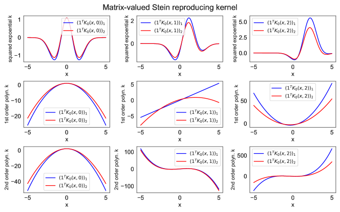
Figure 3: Illustration of a separable mv-kernel $K_{0}$ for $T=2$ through projections with $\bm{1}=(1,1)$. Here, $\Pi_{1}=\mathcal{N}(0,1)$, $\Pi_{2}=\mathcal{N}(0,1.25)$, $B_{11}=B_{22}=1$ and $B_{12}=B_{21}=0.1$. The first row corresponds to taking $k$ to be a squared-exponential kernel, whereas the second and third row correspond to taking a polynomial kernel $k(x,y)=(x^{\top}y+1)^{l}$ with $l=1$ and $l=2$ respectively.

E.2 Additional Experiment: A Synthetic Example

Here is a synthetic example selected from (South et al., 2022b) (denoted $f_{2}$), and to make the problem fit into our framework we introduced another similar integrand (denoted $f_{1}$):

$$\textstyle f_{1}(x)=1.5+x+1.5x^{2}+1.75\sin(\pi x)\exp(-x^{2}),$$

$$\textstyle f_{2}(x)=1+x+x^{2}+\sin(\pi x)\exp(-x^{2}).$$

For this problem, we trained all CV s through stochastic optimisation and use $m=(50,50)$ MC samples. This synthetic example was originally used by (South et al., 2022b) to show one of the drawbacks of kernel-based CV s, namely that the fitted CV will usually tend to $\beta$ in parts of the domain where we do not have any function evaluations. This phenomenon can be observed on the red lines in Figure 4 (left and center) which gives a CV based on a squared-exponential kernel. This behaviour is clearly one of the biggest drawbacks of existing kernel-based approaches. However, the blue curve, representing a kernel-based vv-CV with separable kernel where $B$ was inferred through optimisation, partially overcomes this issue by using evaluations of both integrands, hence clearly demonstrating potential advantages of sharing function values across integration tasks.

The right-most plot in Figure 4 presents several box plots for the sum of squared errors for each integration problem calculated over $100$ repetitions of the experiment. The different box plots show the impact of the difference in $\Pi_{1}$ and $\Pi_{2}$. As we observed, vv-CV s tend to outperform CV s, although this difference in performance is more stark when $\Pi_{2}$ has a larger tail than $\Pi_{1}$. This reinforces the previous point, since a more disperse $\Pi_{2}$ means that the second integrand will be evaluated more often at more extreme areas of the domain, which will help obtain a better vv-CV by improving the fit at the tails of the distribution.

In this experiment, the choice of $k$ as a squared-exponential kernel was motivated by the fact that this makes $k_{0}$ infinitely differentiable, and hence matching the smoothness of both $f_{1}$ and $f_{2}$.

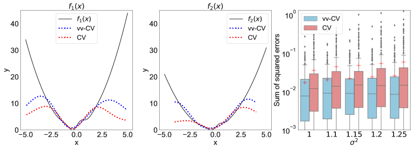
Figure 4: Numerical integration of problem from (South et al., 2022b). Left and center: Illustration of $f_{1}$ and $f_{2}$, as well as the corresponding kernel-based CV s and vv-CV s obtained through stochastic optimisation when $\Pi_{1}=\mathcal{N}(0,1)$ and $\Pi_{2}=\mathcal{N}(0,1.25)$. Right: Sum of the squared errors in estimating $\Pi_{1}[f_{1}]$ and $\Pi_{2}[f_{2}]$. Here, $\Pi_{1}=\mathcal{N}(0,1)$ whilst $\Pi_{2}=\mathcal{N}(0,\sigma^{2})$ where $\sigma^{2}\in\{1,1.1,1.15,1.2,1.25\}$.

The experiment was replicated $100$ times for all methods. The exact details of the implementation are as follows.

• CV

  • Sample size: $50$.

  • Hyper-parameter tuning: batch size $5$; learning rate $0.05$; total number of epochs $30$.

  • Base kernel: squared exponential kernel

  • Optimisation: $\lambda=0.001$; batch size is $5$; learning rate is $0.001$; total number of epochs $400$.

• vv-CV (estimated $B$)

  • Sample size: $(50,50)$ from $(\Pi_{1},\Pi_{2})$ for $(f_{1},f_{2})$.

  • Hyper-parameter tuning: batch size $5$ ($10$ in total for $(f_{1},f_{2})$); learning rate $0.05$; total number of epochs $30$.

  • Base kernel: squared exponential kernel

  • Optimisation: $B^{(0)}$ is initialized at the identity matrix $I_{2}$. $\lambda=0.001$; batch size is $5$ ($10$ in total for $(f_{1},f_{2})$); learning rate is $0.001$; total number of epochs $400$.

E.3 Experimental details of Multi-fidelity Univariate Step Functions

The experiment is replicated $100$ times for all methods. Details of their implementation is given below:

• Squared-exponential kernel

  • CV

    • Sample size: $40$.

    • Base kernel: squared exponential kernel.

    • Hyper-parameter tuning: batch size is $10$; learning rate $0.02$; total number of epochs $15$.

    • Optimisation: $\lambda=1e-5$; batch size is $10$; learning rate is $3e-4$; total number of epochs $400$.

  • vvCV (estimated B/fixed B)

    • Sample size: $(40,40)$ from $(\text{Normal}(0,1),\text{Normal}(0,1))$ for $(f_{L},f_{H})$.

    • Hyper-parameter tuning: batch size is $5$ ($10$ in total for $(f_{L},f_{H})$); learning rate $0.02$; total number of epochs $15$.

    • Base kernel: squared exponential kernel.

    • Optimisation: When $B$ is fixed, we set $B_{11}=B_{22}=0.5,B_{12}=B_{21}=0.01$; otherwise, $B^{(0)}$ is initialized at the identity matrix $I_{2}$. $\lambda=1e-5$; batch size is $5$ ($10$ in total for $(f_{L},f_{H})$); learning rate is $3e-4$; total number of epochs $400$.

• First-order polynomial kernel

  • CV

    • Sample size: $40$.

    • Base kernel: first order polynomial kernel.

    • Optimisation: $\lambda=10^{-5}$; batch size is $10$; learning rate is $3\times 10^{-4}$; total number of epochs $400$.

  • vv-CV (estimating B/fixed B)

    • Sample size: $(40,40)$ from $(\text{Normal}(0,1),\text{Normal}(0,1))$ for $(f_{L},f_{H})$.

    • Base kernel: first order polynomial kernel.

    • Optimisation: When $B$ is fixed, we set $B_{11}=B_{22}=0.5,B_{12}=B_{21}=0.01$; otherwise, $B^{(0)}$ is initialized at the identity matrix $I_{2}$. $\lambda=10^{-5}$; batch size is $5$ ($10$ in total for $(f_{L},f_{H})$); learning rate is $3\times 10^{-4}$; total number of epochs $400$.

The empirical computational cost for all tasks is as follows. Scalar-valued CVs take approximately $2.4$ seconds for either choice of kernels; vv-CV s with fixed $B$ take around $3.3$ seconds with a squared-exponential kernel or around $3.1$ seconds with a $1$st order polynomial kernel; vv-CV s with estimated $B$ take around $6.6$ seconds with a squared-exponential kernel or around $6.2$ seconds with a $1$st order polynomial kernel.

E.4 Experimental Details of the Physical Modelling (Borehole) of Waterflow

Table 4: Prior Distributions for the inputs of the Borehole function.

Random variable	Distributions	Random variable	Distributions
$r_{w}$	$\text{Normal}(0.1,0.0161812^{2})$	$r$	$\text{Normal}(100,0.01)$
$T_{u}$	$\text{Normal}(89335,20)$	$T_{l}$	$\text{Normal}(89.55,1)$
$H_{u}$	$\text{Normal}(1050,1)$	$H_{l}$	$\text{Normal}(760,1)$
$L$	$\text{Normal}(1400,10)$	$K_{w}$	$\text{Normal}(10950,30)$

In this section, we provide details on the Borehole example from the main paper, and provide complementary experiments. The distributions with respect to which the integral is taken is an eight-dimensional Gaussian with independent marginals provided in Table 4. The low-fidelity model and high-fidelity model of water flow (Xiong et al., 2013) is given by,

$$\textstyle f_{L}(x)=\frac{5T_{u}(H_{u}-H_{l})}{\log\left(\frac{r}{r_{w}}\right)\Big{(}1.5+\frac{2LT_{u}}{\log\left(\frac{r}{r_{w}}\right)r_{w}^{2}K_{w}}+\frac{T_{u}}{T_{l}}\Big{)}}$$

$$\textstyle f_{H}(x)=\frac{2\pi T_{u}(H_{u}-H_{l})}{\log\left(\frac{r}{r_{w}}\right)\Big{(}1+\frac{2LT_{u}}{\log\left(\frac{r}{r_{w}}\right)r_{w}^{2}K_{w}}+\frac{T_{u}}{T_{l}}\Big{)}}.$$

where $x=(r_{w},r,T_{u},T_{l},H_{u},H_{l},L,K_{w})$.

E.4.1 Experiment in the main text: Balanced vv-CVs

The number of replications is $100$ for all methods. Details of their implementation is given below:

• Base kernel: Instead of using $k(x,x^{\prime})=\exp(-\|x-x^{\prime}\|_{2}^{2}/2\nu)$ with $l>0$ which implicitly assumes that the length-scales are identical in all directions, we now allow that each dimension can have its own length-scale. That is,

  $$\textstyle k(x,x^{\prime}):=\prod_{j=1}^{d}k_{j}(x_{j},x^{\prime}_{j})\qquad\text{ where }\qquad k_{j}(x_{j},x^{\prime}_{j})=\exp\left(-\frac{(x_{j}-x^{\prime}_{j})_{2}^{2}}{2\nu_{j}}\right).$$

  Each of the components has its own length-scale $\nu_{j}>0$ to be determined.

• Since $\pi(x)=\prod_{j=1}^{d}\pi_{j}(x_{j})$, the score function is $\nabla_{x}\log\pi(x)=\left(\frac{\partial\log\pi_{1}(x)}{\partial x_{1}},\ldots,\frac{\partial\log\pi_{d}(x)}{\partial x_{d}}\right)^{\top}.$

• Hyper-parameter tuning: batch size $5$ ($10$ in total for $(f_{L},f_{H})$); learning rate of tuning $0.05$; epochs of tuning $20$.

• Optimisation (estimated B/pre-fixing B): When $B$ is fixed, we set $B_{11}=B_{22}=5e-4,B_{12}=B_{21}=5e-5$; otherwise, $B^{(0)}$ is initialized at $1e-5\times I_{2}$. $\lambda=1e-5$; batch size $5$ ($10$ in total for $(f_{L},f_{H})$); learning rate for the cases when sample sizes are $(10,20,50,100,150)$ are $(0.09,0.06,0.012,0.0035,0.002)$, respectively.

The empirical computational cost (measured in seconds) of this example is: when $m=(10,10)$, it takes CF, vv-CV s with fixed B and vv-CV s with estimated B around $0.03$, $1.2$ and $2.6$ seconds, respectively; when $m=(20,20)$, it takes CF, vv-CV s with fixed B and vv-CV s with estimated B around $0.1$, $3$ and $5$ seconds, respectively; when $m=(50,50)$, it takes CF, vv-CV s with fixed B and vv-CV s with estimated B around $0.7$, $7.5$ and $13.5$ seconds, respectively; when $m=(100,100)$, it takes CF, vv-CV s with fixed B and vv-CV s with estimated B around $2.7$, $17$ and $27.6$ seconds, respectively; when $m=(150,150)$, it takes CF, vv-CV s with fixed B and vv-CV s with estimated B around $6$, $29$ and $49$ seconds, respectively.

E.4.2 Additional Experiment: Unbalanced Data-sets for Physical Modelling of Waterflow

In Figure 5, we present the results of vv-CVs when the sample sizes are unbalanced; that is, we have a different number of samples for the low-fidelity and high-fidelity models. The exact setup is given below, and we replicated the experiment $100$ times.

• Sample size: $m_{H}$ is fixed to be $20$, while $m_{L}\in\{20,40,60\}$.

• Base kernel: product of squared exponential kernels. $k(x,x^{\prime}):=\prod_{j=1}^{d}k_{j}(x_{j},x^{\prime}_{j})$, where each $k_{j}(x_{j},x^{\prime}_{j})=\exp(-(x_{j}-x^{\prime}_{j})_{2}^{2}/2\nu_{j})$ has its own length-scale $\nu_{j}>0$ to be determined.

• Hyperparameter tuning: batch size of tuning $5$ ($10$ in total for $(f_{L},f_{H})$); learning rate of tuning is $0.05$; epochs of tuning is $20$.

• Optimisation (estimated B/pre-fixing B): When $B$ is fixed, we set $B_{11}=B_{22}=5\times 10^{-4},B_{12}=B_{21}=5\times 10^{-5}$; otherwise, $B^{(0)}$ is initialized at $10^{-5}\times I_{2}$. $\lambda=10^{-5}$; learning rate is $(0.06,0.04,0.02)$ when $m_{L}\in\{20,40,60\}$, respectively.

Interestingly, we notice that not much is gained when increasing the number of samples for the low-fidelity model. In fact, in the case of a fixed $B$, the performance tends to decrease with a larger $m_{L}$. This is likely due to the “negative transfer” phenomenon which is well-known in machine learning. This phenomenon can occur when two tasks are not similar enough to provide any gains in accuracy. In this case, there is clearly no advantage in using a larger $m_{L}$ since this increases computational cost and does not provide any gains in accuracy.

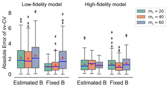
Figure 5: Performance of vv-CVs with unbalanced sample sizes. Here we fix $m_{H}=20$, and changing $m_{L}$ to be $20,40,60$. Each experiment is repeated 100 times.

E.5 Experimental Details of the Computation of the Model Evidence through Thermodynamic Integration

To implement our vv-CV s, we need to derive the corresponding score functions. For a power posterior, the score function is of the form:

$$\textstyle\nabla_{\theta}\log p(\theta|y,t)=t\nabla_{\theta}\log p(y|\theta)+\nabla_{\theta}\log p(\theta)$$

where $\nabla_{\theta}\log p(\theta)$ is the score function corresponding to the prior. In our case, the prior is a log-normal distribution $\log\theta\sim\mathcal{N}(\mu,\sigma^{2})$ (where $\sigma=0.25$), and its score function is given by:

$$\textstyle\nabla_{\theta}\log p(\theta) \textstyle=-\frac{1}{\theta}-\frac{\log\theta-\mu}{x\sigma^{2}}.$$

The score functions for all temperatures are plotted in Figure 6; as observed, temperatures consecutive score functions are very similar to one another.

In order to keep the computational cost manageable, we split the $T=62$ integration problems into groups of closely related problems. In particular, we jointly estimate the means in terms of $4$ consecutive temperatures on the ladder ( group 1 is $\mu_{1},\mu_{2},\mu_{3},\mu_{4}$, group 2 is $\mu_{5},\mu_{6},\mu_{7},\mu_{8}$, etc…). Since $31$ is not divisible by $4$, our last group consists of three means $\mu_{29},\mu_{30},\mu_{31}$. Then, the same approach is taken to create groups of 4 (or 3 for the last group) variances.

The number of replications was $20$ for each method. Details are given below:

• CV

  • Base kernel: Preconditioned squared-exponential kernel (Oates et al., 2017).

  • Hyperparameter tuning: we use the values $(0.1,3)$ in (Oates et al., 2017).

  • Optimisation: $\lambda=10^{-3}$; batch size is $5$; total number of epochs is $400$.

• vv-CV(estimated B)

  • Base kernel: Preconditioned squared-exponential kernel (Oates et al., 2017).

  • Hyperparameter tuning: we use the values $(0.1,3)$ in (Oates et al., 2017).

  • Optimisation: $\lambda=10^{-3}$; batch size is $5$; learning rate is $0.01$; number of epochs is $400$.

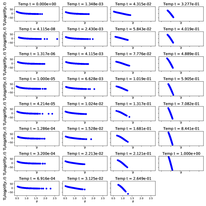
Figure 6: Score functions corresponding to the power posteriors at different temperatures on the temperature ladder.

E.6 Experimental Details of the Lotka-Volterra System

We implement $\log$-$\exp$ transform on model parameters and avoid constrained parameters on the ODE directly. Lotka—Volterra system can be re-parameterized as,

$$\textstyle\frac{dv_{1}(s)}{ds} \textstyle=\tilde{\alpha}v_{1}(s)-\tilde{\beta}v_{1}(s)v_{2}(s)$$

$$\textstyle\frac{dv_{2}(s)}{ds} \textstyle=\tilde{\delta}v_{1}(s)v_{2}(s)-\tilde{\gamma}v_{2}(s),$$

where

$$\textstyle\tilde{\alpha}=\exp(\alpha),\tilde{\beta}=\exp(\beta),$$

$$\textstyle\tilde{\delta}=\exp(\delta),\tilde{\gamma}=\exp(\gamma),$$

where $v_{1}$ and $v_{2}$ represents the number of preys and predators, respectively.

The model is,

$$\textstyle y_{10}\sim\text{Log-Normal}(\log\tilde{v}_{1}(0),\tilde{\sigma}_{y_{1}})$$

$$\textstyle y_{20}\sim\text{Log-Normal}(\log\tilde{v}_{2}(0),\tilde{\sigma}_{y_{2}})$$

$$\textstyle y_{1s}\sim\text{Log-Normal}(\log v_{1}(s),\tilde{\sigma}_{y_{1}})$$

$$\textstyle y_{2s}\sim\text{Log-Normal}(\log v_{2}(s),\tilde{\sigma}_{y_{2}})$$

where

$$\textstyle\tilde{v}_{1}(0):=\exp(v_{1}(0)),\tilde{v}_{2}(0):=v_{2}(0)$$

$$\textstyle\tilde{\sigma}_{y_{1}}:=\exp(\sigma_{y_{1}}),\tilde{\sigma}_{y_{2}}=\exp(\sigma_{y_{2}}).$$

By doing so, $x:=(\alpha,\beta,\delta,\gamma,v_{1}(0),v_{2}(0),\sigma_{x},\sigma_{y})^{\top}$ can be defined on the whole $\mathbb{R}^{8}$ as the exponential transformation will make sure they larger than zero, and thus can be assigned priors on $\mathbb{R}^{8}$, e.g., Gaussian. As a result, the expectations asscoiated with $\pi(x)$ are defined on $\mathbb{R}^{8}$ and Stan will return the scores of these parameters directly as these 8 parameters $x$ themselves are unconstrained through manually reparameterisation.

Priors are,

$$\textstyle\alpha,\gamma \textstyle\sim\text{Normal}(0,0.5^{2})$$

$$\textstyle\beta,\delta \textstyle\sim\text{Normal}(-3,0.5^{2})$$

$$\textstyle\sigma_{x},\sigma_{y} \textstyle\sim\text{Normal}(-1,1^{2})$$

$$\textstyle v_{1}(0),v_{2}(0) \textstyle\sim\text{Normal}(\log 10,1^{2})$$

The fitting for predators $y_{1s}$ and $v_{1}(s)$ at points $s_{1},\ldots,s_{m}$ are shown in Figure 7. The fitting for predators $y_{2s}$ and $v_{2}(s)$ at points $s_{1},\ldots,s_{m}$ are shown in Figure 8.

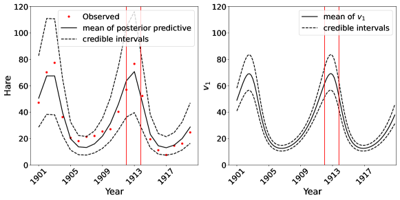
Figure 7: Bayesian inference of abundance of preys of Lotka-Volterra system. Dots are observations; lines are the posterior means while dotted lines are the corresponding $95\%$ credible intervals. Tasks are chosen in the area between the two vertical red lines.

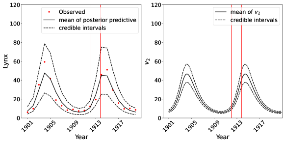
Figure 8: Bayesian inference of abundance of predators of Lotka-Volterra system. Dots are observations; lines are the posterior means while dotted lines are the corresponding $95\%$ credible intervals. Tasks are chosen in the area between the two vertical red lines.

The number of replications is $10$ for each method and for each task. Details are given below:

• Tasks $\Pi[f_{t}]$ at time $s_{1}^{\prime},\ldots,s_{T}^{\prime}$ (the base unit is $1$ year):

  • $T=2$: $1913.,1913.2$;

  • $T=5$: $1912.,1912.2,1912.4,1912.6,1912.8$;

  • $T=10$: $1912.,1912.2,1912.4,1912.6,1912.8,1913.,1913.2,1913.4,1913.6,1913.8$.

• Base kernel: same one as in E.4: product of squared-exponential kernels.

• Hyperparameter tuning: batch size is $10$; learning rate $0.01$; total number of epochs $10$.

• Optimisation: $\lambda=10^{-5}$; batch size $10$; learning rate $10^{-3}$; total number of epochs $400$.

The empirical computational cost (measured in seconds) of this example is: when $T=2$, it takes CF, scalar-valued CVs, vv-CV s with fixed B and vv-CV s with estimated B around $67$, $80$, $150$ and $159$ seconds respectively for all $T$ tasks; when $T=5$, it takes CF, scalar-valued CVs, vv-CV s with fixed B and vv-CV s with estimated B around $170$, $200$, $854$ and $882$ seconds respectively for all $T$ tasks; when $T=10$, it takes CF, scalar-valued CVs, vv-CV s with fixed B and vv-CV s with estimated B around $340$, $400$, $3435$ and $3469$ seconds respectively for all $T$ tasks.

E.6.1 Addition Experiments for Bayesian inference of abundance of preys of Lotka-Volterra system

We present additional experiments in Table 5 under the same settings as those in the above section. We consider to estimate $\Pi[f_{t}]$ at time $s_{1}^{\prime},\ldots,s_{T}^{\prime}$ (the base unit is $1$ year),

• $T=2$: $1915.,1915.2$;

• $T=5$: $1915.,1915.2,1915.4,1915.6,1915.8$;

• $T=10$: $1914.,1914.2,1914.4,1914.6,1914.8,1915.,1915.2,1915.4,1915.6,1915.8$.

Table 5: Additional Experiments for the Bayesian inference of the Lotka-Volterra system: Sum of mean absolute error of each task.

$T$	$m$	vv-CV- Estimated B	vv-CV-Fixed B	CF	MC
2	$500$	0.169	0.144	0.242	0.275
5	$500$	0.322	0.245	1.246	0.661
10	$500$	0.916	0.792	5.835	1.797

References

- Álvarez et al. (2012) Álvarez, M. A., Rosasco, L., and Lawrence, N. D. Kernels for vector-valued functions: A review. Foundations and Trends in Machine Learning, 4(3):195–266, 2012.
- Anastasiou et al. (2023) Anastasiou, A., Barp, A., Briol, F.-X., Ebner, B., Gaunt, R. E., Ghaderinezhad, F., Gorham, J., Gretton, A., Ley, C., Liu, Q., Mackey, L., Oates, C. J., Reinert, G., and Swan, Y. Stein’s method meets Statistics: A review of some recent developments. Statistical Science, 38(1):120–139, 2023.
- Assaraf & Caffarel (1999) Assaraf, R. and Caffarel, M. Zero-variance principle for Monte Carlo algorithms. Physical Review Letters, 83(23):4682, 1999.
- Barp et al. (2021) Barp, A., Takao, S., Betancourt, M., Arnaudon, A., and Girolami, M. A unifying and canonical description of measure-preserving diffusions. arXiv preprint arXiv:2105.02845, 2021.
- Barp et al. (2022a) Barp, A., Oates, C. J., Porcu, E., and Girolami, M. A riemann–stein kernel method. Bernoulli, 28(4):2181–2208, 2022a.
- Barp et al. (2022b) Barp, A., Simon-Gabriel, C.-J., Girolami, M., and Mackey, L. Targeted separation and convergence with kernel discrepancies. arXiv preprint arXiv:2209.12835, 2022b.
- Berlinet & Thomas-Agnan (2011) Berlinet, A. and Thomas-Agnan, C. Reproducing Kernel Hilbert Spaces in Probability and Statistics. Springer Science & Business Media, 2011.
- Bottou et al. (2018) Bottou, L., Curtis, F. E., and Nocedal, J. Optimization methods for large-scale machine learning. SIAM Review, 60(2):223–311, 2018. ISSN 00361445. doi: 10.1137/16M1080173.
- Briol et al. (2017) Briol, F.-X., Oates, C. J., Cockayne, J., Chen, W. Y., and Girolami, M. On the sampling problem for kernel quadrature. In Proceedings of the International Conference on Machine Learning, pp. 586–595, 2017.
- Calderhead & Girolami (2009) Calderhead, B. and Girolami, M. Estimating Bayes factors via thermodynamic integration and population MCMC. Computational Statistics and Data Analysis, 53(12):4028–4045, 2009.
- Carmeli et al. (2006) Carmeli, C., De Vito, E., and Toigo, A. Vector valued reproducing kernel Hilbert spaces of integrable functions and Mercer theorem. Analysis and Applications, 4(4):377–408, 2006.
- Carmeli et al. (2010) Carmeli, C., De Vito, E., Toigo, A., and Umanita, V. Vector valued reproducing kernel Hilbert spaces and universality. Analysis and Applications, 8(1):19–61, 2010.
- Carpenter et al. (2017) Carpenter, B., Gelman, A., Hoffman, M. D., Lee, D., Goodrich, B., Betancourt, M., Brubaker, M., Guo, J., Li, P., and Riddell, A. Stan: A probabilistic programming language. Journal of statistical software, 76(1), 2017.
- Ciliberto et al. (2015) Ciliberto, C., Mroueh, Y., Poggio, T., and Rosasco, L. Convex learning of multiple tasks and their structure. In International Conference on Machine Learning, pp. 1548–1557, 2015.
- Dellaportas & Kontoyiannis (2012) Dellaportas, P. and Kontoyiannis, I. Control variates for estimation based on reversible Markov chain Monte Carlo samplers. Journal of the Royal Statistical Society Series B: Statistical Methodology, 74(1):133–161, 2012.
- Dinuzzo et al. (2011) Dinuzzo, F., Ong, C. S., Gehler, P. V., and Pillonetto, G. Learning output kernels with block coordinate descent. In International Conference on Machine Learning, 2011.
- Evgeniou et al. (2005) Evgeniou, T., Micchelli, C. A., and Pontil, M. Learning multiple tasks with kernel methods. Journal of Machine Learning Research, 6:615–637, 2005.
- Friel & Pettitt (2008) Friel, N. and Pettitt, A. N. Marginal likelihood estimation via power posteriors. Journal of the Royal Statistical Society: Series B (Statistical Methodology), 70(3):589–607, 2008.
- Friel et al. (2014) Friel, N., Hurn, M., and Wyse, J. Improving power posterior estimation of statistical evidence. Statistics and Computing, 24(5):709–723, 2014.
- Girolami & Calderhead (2011) Girolami, M. and Calderhead, B. Riemann manifold Langevin and Hamiltonian Monte Carlo methods. Journal of the Royal Statistical Society Series B: Statistical Methodology, 73(2):123–214, 2011.
- Green et al. (2015) Green, P., Latuszyski, K., Pereyra, M., and Robert, C. Bayesian computation: a summary of the current state, and samples backwards and forwards. Statistics and Computing, 25:835–862, 2015.
- Hewitt (1921) Hewitt, C. G. The conservation of the wild life of Canada. New York: C. Scribner, 1921.
- Hickernell et al. (2005) Hickernell, F. J., Lemieux, C., and Owen, A. B. Control variates for quasi-Monte Carlo. Statistical Science, 20(1):1–31, 2005.
- Jones (2004) Jones, G. L. On the Markov chain central limit theorem. Probability Surveys, 1:299–320, 2004.
- Kandasamy et al. (2016) Kandasamy, K., Dasarathy, G., Oliva, J., Schneider, J., and Poczos, B. Gaussian process optimisation with multi-fidelity evaluations. In Neural Information Processing Systems, pp. 992–1000, 2016.
- Kingma & Ba (2015) Kingma, D. P. and Ba, J. L. Adam: A method for stochastic optimization. In International Conference on Learning Representations, 2015.
- Leluc et al. (2021) Leluc, R., Portier, F., and Segers, J. Control variate selection for monte carlo integration. Statistics and Computing, 31(4):1–27, 2021.
- Lotka (1925) Lotka, A. J. Elements of physical biology. Williams & Wilkins, 1925.
- Lotka (1927) Lotka, A. J. Fluctuations in the abundance of a species considered mathematically. Nature, 119(2983):12–12, 1927.
- Micchelli & Pontil (2005) Micchelli, C. A. and Pontil, M. On learning vector-valued functions. Neural Computation, 17(1):177–204, 2005.
- Mijatovic & Vogrinc (2018) Mijatovic, A. and Vogrinc, J. On the Poisson equation for Metropolis-Hastings chains. Bernoulli, 24(3):2401–2428, 2018. ISSN 13507265.
- Mira et al. (2013) Mira, A., Solgi, R., and Imparato, D. Zero variance Markov chain Monte Carlo for Bayesian estimators. Statistics and Computing, 23(5):653–662, 2013.
- Oates & Girolami (2016) Oates, C. J. and Girolami, M. Control functionals for quasi-Monte Carlo integration. In Proceedings of the International Conference on Artificial Intelligence and Statistics, volume 51, pp. 56–65, 2016.
- Oates et al. (2016) Oates, C. J., Papamarkou, T., and Girolami, M. The controlled thermodynamic integral for Bayesian model comparison. Journal of the American Statistical Association, 111(514):634–645, 2016.
- Oates et al. (2017) Oates, C. J., Girolami, M., and Chopin, N. Control functionals for Monte Carlo integration. Journal of the Royal Statistical Society: Series B (Statistical Methodology), 79(3):695–718, 2017.
- Oates et al. (2019) Oates, C. J., Cockayne, J., Briol, F.-X., Girolami, M., et al. Convergence rates for a class of estimators based on Stein’s method. Bernoulli, 25(2):1141–1159, 2019.
- Papamarkou et al. (2014) Papamarkou, T., Mira, A., and Girolami, M. Zero variance differential geometric Markov chain Monte Carlo algorithms. Bayesian Analysis, 9(1):97–128, 2014.
- Park et al. (2017) Park, C., Haftka, R. T., and Kim, N. H. Remarks on multi-fidelity surrogates. Structural and Multidisciplinary Optimization, 55(3):1029–1050, 2017.
- Peherstorfer et al. (2018) Peherstorfer, B., Willcox, K., and Gunzburger, M. Survey of multifidelity methods in uncertainty propagation, inference, and optimization. SIAM Review, 60(3):550–591, 2018.
- Si et al. (2021) Si, S., Oates, C. J., Duncan, A. B., Carin, L., and Briol, F.-X. Scalable control variates for Monte Carlo methods via stochastic optimization. Proceedings of the 14th Conference on Monte Carlo and Quasi-Monte Carlo Methods. arXiv:2006.07487, 2021.
- South et al. (2022a) South, L. F., Karvonen, T., Nemeth, C., Girolami, M., and Oates, C. J. Semi-exact control functionals from Sard’s method. Biometrika, 109(2):351–367, 2022a.
- South et al. (2022b) South, L. F., Riabiz, M., Teymur, O., and Oates, C. J. Post-Processing of MCMC. Annual Review of Statistics and Its Application, 2022b.
- Steinwart & Christmann (2008) Steinwart, I. and Christmann, A. Support vector machines. Springer Science & Business Media, 2008.
- Sun et al. (2023) Sun, Z., Oates, C. J., and Briol, F.-X. Meta-learning control variates: Variance reduction with limited data. arXiv:2303.04756, to appear at UAI, 2023.
- Volterra (1926) Volterra, V. Variazioni e fluttuazioni del numero d’individui in specie animali conviventi. Società anonima tipografica” Leonardo da Vinci”, 1926.
- Wan et al. (2019) Wan, R., Zhong, M., Xiong, H., and Zhu, Z. Neural control variates for variance reduction. Joint European Conference on Machine Learning and Knowledge Discovery in Databases, pp. 533–547, 2019.
- Xi et al. (2018) Xi, X., Briol, F.-X., and Girolami, M. Bayesian quadrature for multiple related integrals. In International Conference on Machine Learning, pp. 5373–5382, 2018.
- Xiong et al. (2013) Xiong, S., Qian, P. Z. G., and Wu, C. F. J. Sequential design and analysis of high-accuracy and low-accuracy computer codes. Technometrics, 55(1):37–46, 2013.