Complex Temporal Question Answering on Knowledge Graphs

Abstract.

Question answering over knowledge graphs (KG-QA) is a vital topic in IR. Questions with temporal intent are a special class of practical importance, but have not received much attention in research. This work presents Exaqt, the first end-to-end system for answering complex temporal questions that have multiple entities and predicates, and associated temporal conditions. Exaqt answers natural language questions over KGs in two stages, one geared towards high recall, the other towards precision at top ranks. The first step computes question-relevant compact subgraphs within the KG, and judiciously enhances them with pertinent temporal facts, using Group Steiner Trees and fine-tuned BERT models. The second step constructs relational graph convolutional networks (R-GCNs) from the first step’s output, and enhances the R-GCNs with time-aware entity embeddings and attention over temporal relations. We evaluate Exaqt on TimeQuestions, a large dataset of $16k$ temporal questions we compiled from a variety of general purpose KG-QA benchmarks. Results show that Exaqt outperforms three state-of-the-art systems for answering complex questions over KGs, thereby justifying specialized treatment of temporal QA.

1. Introduction

Motivation. Questions and queries with temporal information needs (Kanhabua and Anand, 2016; Alonso et al., 2011; Alonso et al., 2007; Berberich et al., 2010; Campos et al., 2014) represent a substantial use case in search. For factual questions, knowledge graphs (KGs) like Wikidata (Vrandečić and Krötzsch, 2014), YAGO (Suchanek et al., 2007), or DBpedia (Auer et al., 2007), have become the go-to resource for search engines, tapping into structured facts on entities. While question answering over KGs (Bast and Haussmann, 2015; Bhutani et al., 2019; Saha Roy and Anand, 2020; Yahya et al., 2013; Abujabal et al., 2018; Vakulenko et al., 2019; Berant et al., 2013; Yih et al., 2015; Diefenbach et al., 2019) has been a major topic, little attention has been paid to the case of temporal questions. Such questions involve explicit or implicit notions of constraining answers by associated timestamps in the KG. This spans a spectrum, starting from simpler cases such as when was obama born?, where did obama live in 2001?, and where did obama live during 9/11? to more complex temporal questions like:

where did obama’s children study when he became president?

Complex questions must consider multi-hop constraints (Barack Obama $\mapsto$ child $\mapsto$ Malia Obama, Sasha Obama $\mapsto$ educated at $\mapsto$ Sidwell Friends School), and reason on the overlap of the intersection of time points and intervals (the start of the presidency in 2009 with the study period at the school, 2009 – 2016). A simplified excerpt of the relevant zone in the Wikidata KG necessary for answering the question, is shown in Fig. 1. This paper addresses these challenges that arise for complex temporal questions.

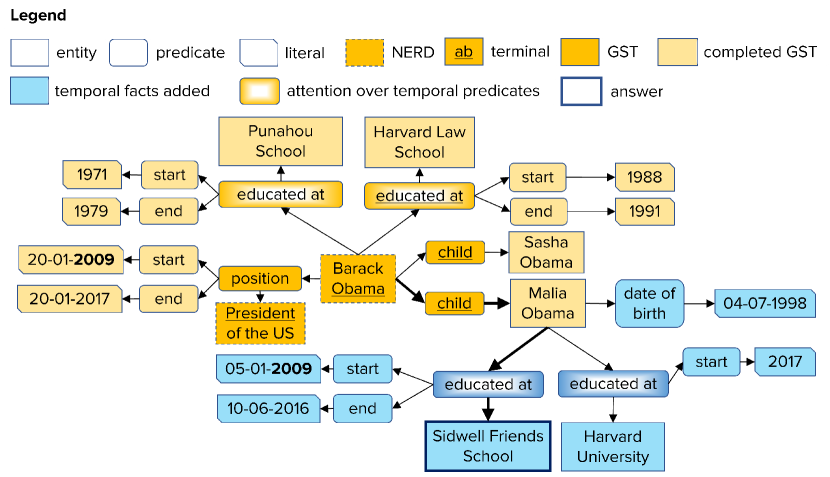
Figure 1. Wikidata excerpt showing the relevant KG zone for the question where did obama’s children study when he became president? with answer Sidwell Friends School.

Limitations of state-of-the-art. Early works on temporal QA over unstructured text sources (Harabagiu and Bejan, 2005; Ahn et al., 2006; Schilder and Habel, 2003; Bruce, 1972; Uzaaman et al., 2012; Pustejovsky et al., 2002; Saquete et al., 2009) involve various forms of question and document parsing, but do not carry over to KGs with structured facts comprised of entities and predicates. The few works specifically geared for time-aware QA over KGs include (Jia et al., 2018b; Costa et al., 2020; Wu et al., 2020). (Jia et al., 2018b) uses a small set of hand-crafted rules for question decomposition and temporal reasoning. This approach needs human experts for the rules and does not cope with complex questions. (Costa et al., 2020) creates a QA collection for KGs that capture events and their timelines. A key-value memory network in (Wu et al., 2020) includes time information from KGs for answering simple questions.

Approach. We present Exaqt: EXplainable Answering of complex Questions with Temporal intent, a system that does not rely on manual rules for question understanding and reasoning. Exaqt answers complex temporal questions in two steps:

• Identifying a compact, tractable answer graph that contains all cues required for answering the question, based on dense-subgraph algorithms and fine-tuned BERT models; and

• A relational graph convolutional network (R-GCN) (Sun et al., 2018) to infer the answer in the graph, augmented with signals about time.

The two stages work as follows (partly illustrated in Fig. 1).

Stage 1: Answer graph construction. Exaqt fetches all KG facts of entities mentioned in the question (Barack Obama, President of the United States: dashed outline boxes), as detected by off-the-shelf NERD systems (Ferragina and Scaiella, 2010; Hoffart et al., 2011; Li et al., 2020). The resulting noisy set of facts is distilled into a tractable set by means of a fine-tuned BERT model (admitting information about the children Malia and Sasha, but not Michelle Obama). To construct a KG subgraph of all question-relevant KG items and their interconnections from this set, Group Steiner Trees (GST) (Shi et al., 2020; Lu et al., 2019; Chanial et al., 2018) are computed (dark orange nodes, terminals or keyword matches underlined: “obama”, “president”, “child”, “educated at”) and completed (light orange nodes). The last and decisive step at this point augments this candidate answer graph with pertinent temporal facts, to bring in cues (potentially multiple hops away from the question entities) about relevant dates, events and time-related predicates. To this end, we use an analogous BERT model for identifying question-relevant temporal facts (blue nodes: educational affiliations of Malia and Sasha and their dates). The resulting answer graph is the input of the second stage.

Stage 2: Answer prediction by R-GCN. Inspired by the popular GRAFT-Net model (Sun et al., 2018) and related work (Schlichtkrull et al., 2018; Sun et al., 2019), we construct an R-GCN that learns entity embeddings over the answer graph and casts answer prediction into a node classification task. However, R-GCNs as used in prior works are ignorant of temporal constraints (Allen, 1983). To overcome this obstacle, we augment the R-GCN with time-aware entity embeddings, attention over temporal relations, and encodings of timestamps (Zhang et al., 2020), temporal signals (Setzer, 2002), and temporal question categories (Jia et al., 2018b). In our running example, temporal attention helps Exaqt focus on educated at as a question-relevant relation (partly shaded nodes). The time-enhanced representation of Barack Obama flows through the R-GCN (thick edges) and boosts the likelihood of Sidwell Friends School as the answer (node with thick borders), which contains 2009 (in bold) among its temporal facts. By producing such concise KG snippets for each question (as colored in Fig. 1), Exaqt yields explainable evidence for its answers.

Contributions. This work makes the following contributions:

• We propose Exaqt, the first end-to-end system for answering complex temporal questions over large-scale knowledge graphs;

• Exaqt applies fine-tuned BERT models and convolutional graph networks to solve the specific challenges of identifying relevant KG facts for complex temporal questions;

• We compile and release TimeQuestions, a benchmark of about $16k$ temporal questions (examples in Table 1);

• Experiments over the full Wikidata KG show the superiority of Exaqt over three state-of-the-art complex KG-QA baselines. All resources from this project are available at https://exaqt.mpi-inf.mpg.de/ and https://github.com/zhenjia2017/EXAQT.

2. Concepts and notation

Category	Question
	who won oscar for best actress 1986?
Explicit	which movie did jaco van dormael direct in 2009?
	what currency is used in germany 2012?
	who was king of france during the ninth crusade?
Implicit	what did thomas jefferson do before he was president?
	what club did cristiano ronaldo play for after manchester united?
	what was the first film julie andrews starred in?
Ordinal	what was the second position held by pierre de coubertin?
	who is elizabeth taylor’s last husband?
	what year did lakers win their first championship?
Temp. Ans.	when was james cagney’s spouse born?
	when was the last time the orioles won the world series?

Table 1. Sample temporal questions from TimeQuestions.

We now define the salient concepts that underlie Exaqt.

Knowledge graph. A knowledge graph (aka knowledge base) is a collection of facts $F$ organized as a set of <subject, predicate, object> triples. It can be stored as an RDF database of such triples, or equivalently as a graph with nodes and edges. Examples are Wikidata (Vrandečić and Krötzsch, 2014), YAGO (Suchanek et al., 2007), DBpedia (Auer et al., 2007), Freebase (Bollacker et al., 2008) and industrial KGs. When stored as a graph, edges are directed: subject $\mapsto$ predicate $\mapsto$ object. Subjects and objects are always nodes, while predicates (aka relations) often become edge labels.

Fact. A fact $f\in F$ can either be binary, containing a subject and an object connected by a predicate, or $n$-ary, combining multiple items via main predicates and qualifier predicates. An example of a binary fact is <Barack Obama, child, Malia Obama>, where subjects are entities (Barack Obama), and objects may be entities (Malia Obama), literals (constants such as dates in <Malia Obama, date of birth, 04-07-1998¿), or types aka classes (private school in <Sidwell Friends School, type, private school>). We use the terms predicate and relation interchangeably in this text.

An $n$-ary fact combines several triples that belong together, such as <Barack Obama, position held, President of the US; start date, 20-01-2009; end date, 20-01-2017> (see Fig. 1). position held is the main predicate, President of the US is the main object, while the remaining data are ¡qualifier predicate, qualifier object¿ pairs. $n$-ary facts are of vital importance in temporal QA, with a large fraction of temporal information in modern KGs being stored as qualifiers. One way of representing qualifiers in a KG is shown in Fig. 1, via paths from the main predicate to the qualifier predicate and on to the qualifier object.

Temporal fact. We define a temporal fact $tf\in F$ as one where the main object or any of the qualifier objects is a timestamp. Examples are <Vietnam War, end date, 30-04-1975> (binary), or, <Steven Spielberg, award received, Academy Award for Best Director; for work, Schindler’s List; point in time, 1993> ($n$-ary).

Temporal predicate. We define a temporal predicate as one that can have a timestamp as its direct object or one of its qualifier objects. Examples are date of birth and position held.

Temporal question. A temporal question is one that contains a temporal expression or a temporal signal, or whose answer is of temporal nature (Jia et al., 2018a). Examples of temporal expressions are “in the year 1998”, “Obama’s presidency”, “New Year’s Eve”, etc. which indicate explicit or implicit temporal scopes (Kuzey et al., 2016). Temporal signals (Setzer, 2002) are markers of temporal relations (BEFORE, AFTER, OVERLAP, ...) (Allen, 1983) and are expressed with words like “prior to, after, during, …” that indicate the need for temporal reasoning. In our models, a question $q$ is represented as a set of keywords ¡$q_{1},q_{2},\ldots q_{|q|}$¿.

Temporal question categories. Temporal questions fall into four basic categories (Jia et al., 2018a): (i) containing explicit temporal expressions (“in 2009”), (ii) containing implicit temporal expressions (“when Obama became president”), (iii) containing temporal ordinals (“first president”), and (iv) having temporal answers (“When did …”). Table 1 gives several examples of temporal questions. A question may belong to multiple categories. For example, what was the first film julie andrews starred in after her divorce with tony walton? contains both an implicit temporal expression and a temporal ordinal.

Answer. An answer to a temporal question is a (possibly singleton) set of entities or literals, e. g., {Chicago University Lab School, Sidwell Friends School} for Where did Malia Obama study before Harvard?, or {08-2017} for When did Malia start at Harvard?

Answer graph. An answer graph is a subset of the KG that contains all the necessary facts for correctly answering the question.

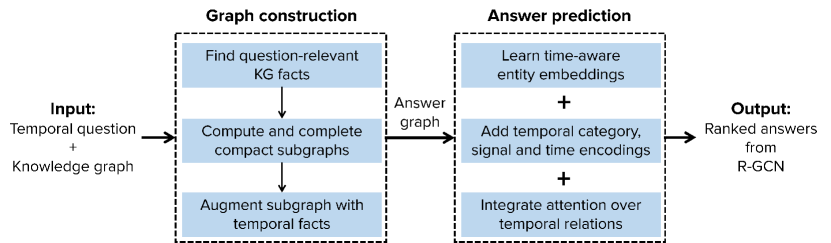
Figure 2. An overview of the two-stage Exaqt pipeline.

3. Constructing answer graphs

Fig. 2 is an overview of Exaqt, with two main stages: (i) answer graph construction (Sec. 3), and (ii) answer prediction (Sec. 4).

3.1. Finding question-relevant KG facts

NERD for question entities. Like most QA pipelines (Qiu et al., 2020; Bhutani et al., 2019), we start off by running named entity recognition and disambiguation (NERD) (Li et al., 2020; van Hulst et al., 2020; Hoffart et al., 2011) on the input question (where did obama’s children study when he became president?). NERD systems identify spans of words in the question as mentions of entities (“obama”, “president”), and link these spans to KG items or Wikipedia articles (which can easily be mapped to popular KGs). The facts of these linked entities (Barack Obama, President of the United States) provide us with a zone in the KG to start looking for the answer. NERD is a critical cog in the QA wheel: entity linking errors leave the main QA pipeline helpless with respect to answer detection. To mitigate this effect, we use two different systems, TagMe and ELQ (Ferragina and Scaiella, 2010; Li et al., 2020), to boost answer recall. Complex questions often contain multiple entity mentions, and accounting for two NERD systems, we could easily have $2-4$ different entities per question. The total number of associated facts can thus be several hundreds or more. To reduce this large and noisy set of facts to a few question-relevant ones, we fine-tune BERT (Devlin et al., 2019) as follows.

Training a classifier for question-relevant facts. For each question in our training set, we run NERD and retrieve all KG facts of the detected entities. We then use a distant supervision mechanism: out of these facts, the ones that contain the gold answer(s) are labeled as positive instances. While several complex questions may not have their answer in the facts of the question entities (multi-hop cases), the ones that do, comprise a reasonable amount of training data for our classifier for question-relevance. Note that facts with qualifiers are also retrieved for the question entities (complete facts where the question entity appears as a subject, object, or qualifier object): this increases our coverage for obtaining positive examples.

For each positive instance, we randomly sample five negative instances from the facts that do not contain the answer. Sampling question-specific negative instances helps learn a more discriminative classifier, as all negative instances are guaranteed to contain at least one entity from the question (say, <Barack Obama, spouse, Michelle Obama>). Using all facts that do not contain an answer would result in severe class imbalance, as this is much higher than the number of positive instances.

We then pool together the ¡question, fact¿ paired positive and negative instances for all training questions. The fact in this pair is now verbalized as a natural language sentence by concatenating its constituents; qualifier statements are joined using “and” (Oguz et al., 2021). For example, the full fact for Obama’s marriage (a negative instance) is: <Barack Obama, spouse, Michelle Obama; start date, 03-10-1992; place of marriage, Trinity United Church of Christ>. This has two qualifiers, and would be verbalized as “Barack Obama spouse Michelle Obama and start date 03-10-1992 and place of marriage Trinity United Church of Christ.”. The questions paired with the verbalized facts, along with the binary ground-truth labels, are fed as training input to a sequence pair classification model for BERT.

Applying the classifier. Following (Devlin et al., 2019), the question and the fact are concatenated with the special separator token [SEP] in between, and the special classification token [CLS] is added in front of this sequence. The final hidden vector corresponding to [CLS], denoted by $\boldsymbol{C}\in\mathbb{R}^{H}$ ($H$ is the size of the hidden state), is considered to be the accumulated representation. Weights $\boldsymbol{W}$ of a classification layer are the only parameters introduced during fine-tuning, where $\boldsymbol{W}\in\mathbb{R}^{K\times H}$, where $K$ is the number of class labels ($K=2$ here, fact is question-relevant or not). $\log(\text{softmax}(\boldsymbol{CW^{T}}))$ is used as the classification loss function. Once the classifier is trained, given a new ¡question, fact¿ pair, it outputs the probability (and the label) of the fact being relevant for the question. We make this prediction for all candidate facts pertinent to a question, and sort them in descending order of this question relevance likelihood. We pick the top scoring facts $\{f_{qrel}\}$ from here as our question-relevant set.

3.2. Computing compact subgraphs

The set of facts $\{f_{qrel}\}$ contains question-relevant facts but is not indicative as to which are a set of coherent KG items that matter for this question, and how they are connected. To this end, we induce a graph as shown in Fig. 1, from the above set of facts where each KG item (entity, predicate, type, literal) becomes a node of its own. Edges run between components of the same fact in the direction mandated in the KG: subject $\mapsto$ predicate $\mapsto$ object for the main fact, and subject $\mapsto$ predicate $\mapsto$ qualifier predicate $\mapsto$ qualifier object for (optional) qualifiers.

Injecting connectivity. BERT selects $\{f_{qrel}\}$ from the facts of a number of entities as detected by our NERD systems. These entities may not be connected to each other via shared KG facts. However, a connected graph is needed so that our subsequent GST and R-GCN algorithms can produce the desired effects. To inject connectivity in the graph induced from BERT facts, we compute the shortest KG path between every pair of question entities, and add these paths to our graph. In case of multiple paths of same length between two entities, they are scored for question-relevance as follows. A KG path is set of facts: a path of length one is made up of one fact (Barack Obama $\mapsto$ position held $\mapsto$ President of the United States), a path of length two is made up of two facts (Barack Obama $\mapsto$ country $\mapsto$ United States of America $\mapsto$ office held by head of state $\mapsto$ President of the United States), and so on. Each candidate path is verbalized as a set of facts (a period separating two facts) and encoded with BERT (Kaiser et al., 2021), and so is the question. These BERT encodings are stored in corresponding [CLS] tokens. We compute the cosine similarity of [CLS](question) with [CLS](path), and add the path with the highest cosine similarity to our answer graph.

GST model. Computing Group Steiner Trees (GST) (Shi et al., 2020; Sun et al., 2021; Pramanik et al., 2021; Lu et al., 2019) has been shown to be an effective mechanism in identifying query-specific backbone structures in larger graphs, for instance, in keyword search over database graphs (Aditya et al., 2002; Ding et al., 2007). Given a subset of nodes in the graph, called terminals, the Steiner Tree (ST) is the lowest-cost tree that connects all terminals. This reduces to the minimum spanning tree problem when all nodes of the graph are terminals, and to the shortest path problem when there are only two terminals. The GST models a more complex situation where the terminals are arranged into groups or sets, and it suffices to find a Steiner Tree that connects at least one node from each group. This scenario fits our requirement perfectly, where each question keyword can match multiple nodes in the graph, and naturally induces a terminal group. Finding a tree that runs through each and every matched node is unrealistic, hence the group model.

Edge costs. An integral part of the GST problem is how to define edge costs. Since edges emanate from KG facts, we leverage question-relevance scores assigned by the classifier of Sec. 3.1: $BERT(f_{qrel})\in[0,1]$, converted to edge costs $1-BERT(f_{qrel})\in[0,1]$.

GST algorithm. There are good approximation algorithms for GSTs (Li et al., 2016; Sun et al., 2021), but QA needs high precision. Therefore, we adopted the fixed-parameter-tractable exact algorithm by Ding et al. (Ding et al., 2007). It iteratively grows and merges smaller trees over the bigger graph to arrive at the minimal trees. Only taking the best tree can be risky in light of spurious connections potentially irrelevant to the question. Thus, we used a top-$k$ variant that is naturally supported by the dynamic programming algorithm of (Ding et al., 2007).

GST completion. As shown in Fig. 1, the GST yields a skeleton connecting the most relevant question nodes. To transform this into a coherent context for the question, we need to complete it with facts from where this skeleton was built. Nodes introduced due to this step are shown in light orange in the figure: dates about the presidency, Obama’s children, and the (noisy) fact about Obama’s education. In case the graph has multiple connected components (still possible as our previous connectivity insertions worked only pairwise over entities), top-$k$ GSTs are computed for each component and the union graph is used for this fact completion step.

Example. We show a simplified example in Fig. 1, where the node Barack Obama matches the question keyword “Obama”, child matches “children”, educated at matches “study”, and President of the United States matches “president”. The educated at nodes connected to Malia and Sasha do not feature here as they are not contained in the facts of Barack Obama, and do not yet feature in our answer graph. We consider exact matches, although not just in node labels but also in the set of aliases present in the KG that list common synonyms of entities, predicates and types. This helps us consider relaxed matches without relying on models like word2vec (Mikolov et al., 2013) or GloVe (Pennington et al., 2014), that need inconvenient thresholding on similarity values as a noisy proxy for synonyms. The GST is shown using dark orange nodes with the associated question keyword matches underlined (denoting the terminal nodes). In experiments, we only consider as terminals NERD matches for entities, and keyword matches with aliases for other KG items. The GST naturally includes the internal nodes and edges necessary to connect the terminals. Note that the graph is considered undirected (equivalently, bidirectional) for the purpose of GST computation.

3.3. Augmenting subgraphs with temporal facts

The final step towards the desired answer graph is to enhance it with temporal facts. Here, we add question-relevant temporal facts of entities in the completed GST. This pulls in temporal information necessary for answering questions that need evidence more than one hop away from the question entities (blue nodes in Fig. 1): <Malia Obama, educated at, Sidwell Friends School; start date, 05-01-2009> (+ noise like Malia’s date of birth). The rationale behind this step is to capture facts necessary for faithfully answering the question, where faithful refers to arriving at the answer not by chance but after satisfying all necessary constraints in the question. For example, the question which oscar did leonardo dicaprio win in 2016? can be answered without temporal reasoning, as he only won one Oscar. We wish to avoid such cases in faithful answering.

To this end, we first retrieve from the KG all temporal facts of each entity in the completed GST. We then use an analogously fine-tuned BERT model for question-relevance of temporal facts. The model predicts, for each temporal fact, its likelihood of containing the answer. It is trained using temporal facts of question entities that contain the answer as positive examples, while negative examples are chosen at random from these temporal facts. To trap multi-hop temporal questions in our net, we explore 2-hop facts of question entities for ground truth answers. A larger neighborhood was not used during the first fine-tuning as the total number of facts in two hops of question entities is rather large, but the count of 2-hop temporal facts is a much more tractable number. Moreover, this is in line with our focus on complex temporal questions. Let the likelihood score for a temporal fact $tf$ of an entity in the completed GST be $BERT(tf_{qrel})$. As before, we take the top scoring $\{tf_{qrel}\}$, add them to the answer graph, that is then passed on to Stage 2.

4. Predicting answers with R-GCN

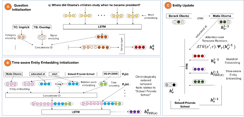
Figure 3. Architecture of the R-GCN model in Exaqt, that includes several signals of temporal information.

R-GCN basics. The answer prediction method of Exaqt is inspired by the Relational Graph Convolution Network model (Schlichtkrull et al., 2018), an extension of GCNs (Duvenaud et al., 2015) tailored for handling large-scale relational data such as knowledge graphs. Typically, a GCN convolves the features (equivalently, representations or embedding vectors) of nodes belonging to a local neighborhood and propagates them to their nearest neighbors. The learned entity representations are used in node classification. Here, this classification decision is whether a node is an answer to the input question or not.

In this work, we use the widely popular GRAFT-Net model (Sun et al., 2018) that adapted R-GCNs to deal with heterogeneous QA over KGs and text (Bhutani and Jagadish, 2019; Oguz et al., 2021). In order to apply such a mechanism for answer prediction in our setup, we convert our answer graph from the previous step into a directed relational graph and build upon the $KG$-only setting of GRAFT-Net. In a relational graph, entities, literals, and types become nodes, while predicates (relations) become edge labels. Specifically, we use the KG RDF dump that contains normal SPO triples for binary facts by employing reification (Hernández et al., 2015). Reified triples can then be straightforwardly represented as a directed relational graph (Sun et al., 2018). Exaqt introduces four major extensions over the R-GCN in GRAFT-Net to deal with the task of temporal QA:

• we embed temporal facts to enrich representations of entity nodes, creating time-aware entity embeddings (TEE);

• we encode temporal question categories (TC) and temporal signals (TS) to enrich question representations;

• we employ time encoding (TE) to obtain the vector representations for timestamps;

• we propose attention over temporal relations (ATR) to distinguish the same relation but with different timestamps as objects.

In the following, we describe how we encode and update the node representations and perform answer prediction in our extended R-GCN architecture for handling temporal questions. Our neural architecture is shown in Fig. 3, while Table 2 summarizes notation for the salient concepts used in this phase.

4.1. Question representation

4.1.1. Initialization

To encode a temporal question, we first determine its temporal category and extract temporal signals (Sec. 2).

Temporal category encoding (TCE). We adopt a noisy yet effective strategy for labeling categories for temporal questions, and leave more sophisticated (multi-label) classification as future work. We use a four-bit multi-hot (recall that a question can belong to multiple categories) vector where each bit indicates whether the question falls into that category. Our tagger works as follows:

• A question is tagged with the “EXPLICIT” category if the annotators SUTime (Chang and Manning, 2012) or HeidelTime (Strötgen and Gertz, 2010) detect an explicit temporal expression inside it;

• A question is tagged with the “IMPLICIT” category if it contains any of the temporal signal words (we used the dictionary compiled by (Setzer, 2002)), and satisfies certain part-of-speech patterns;

• A question is of type “TEMPORAL ANSWER” if it starts with phrases like “when …”, “in which year …”, and “on what date …”;

• A question is tagged with the “ORDINAL” category if it contains an ordinal tag as labeled by the Stanford CoreNLP system (Angeli et al., 2015), along with certain keywords and part-of-speech patterns.

Temporal signal encoding (TSE). There are $13$ temporal relations defined in Allen’s interval algebra for temporal reasoning (Allen, 1983), namely: “equals”, “before”, “meets”, “overlaps”, “during”, “starts”, and “finishes”, with respective inverses for all of them except “equals”. We simplify these relations and adapt the strategy in (Jia et al., 2018a) into $7$ broad classes of temporal signals:

• “before” and “meets” relations are treated as “BEFORE” signals;

• “before-inverse” and “meet-inverse” relations are collapsed into “AFTER” signals;

• “starts” and “finishes” relations are respectively mapped to “START” and “FINISH” signals;

• words with ordinal tags and “last” are mapped to “ORDINAL”;

• all other relations are treated as “OVERLAP” signals;

• absence of any signal word triggers the “NO SIGNAL” case.

We map signal words to temporal signals in questions using a dictionary. We then encode these signals using a $7$-bit (a question can contain multiple signals) vector, where each bit indicates the presence or absence of a particular temporal signal.

Along with these temporal categories and temporal signals, we use a Long Short-Term Memory Network (LSTM) to model the words in the question as a sequence (see block A in Fig. 3). Overall, we represent a question $q$ with $|q|$ words as:

(1) $$\boldsymbol{h^{0}_{q}}=FFN({\boldsymbol{TCE(q)}}\oplus{\boldsymbol{TSE(q)}}\oplus LSTM(\boldsymbol{w_{1}},...,\boldsymbol{w_{|q|}}))$$

Here $\boldsymbol{TCE(q)}$ and $\boldsymbol{TSE(q)}$ are multi-hot vectors encoding the temporal categories and temporal signals present in $q$, and $\boldsymbol{w_{i}}$ represent the pre-trained word embeddings (from Wikipedia2Vec (Yamada et al., 2020)) of the $i^{th}$ word in $q$. We concatenate ($\oplus$) the $\boldsymbol{TCE(q)}$ and $\boldsymbol{TSE(q)}$ vectors with the output vector from the final state of the LSTM. Finally, we pass this concatenated vector through a Feed Forward Network (FFN) and obtain the initial embedding of $q$, denoted as $\boldsymbol{h^{0}_{q}}$.

4.1.2. Update

In subsequent layers, the embedding of the question gets updated with the embeddings of the entities belonging to it (i.e. the question entities obtained from NERD) as follows:

(2) $$\boldsymbol{h^{l}_{q}}=FFN(\sum_{e\in NERD(q)}\boldsymbol{h^{l-1}_{e}})$$

where $NERD(q)$ contains the entities for question $q$ and $\boldsymbol{h^{l-1}_{e}}$ denotes the embedding of an entity $e$ at layer $l-1$.

4.2. Entity representation

4.2.1. Initialization

For initializing each entity $e$ in the relational graph, we use fixed-size pre-trained embeddings $\boldsymbol{x_{e}}$, also from Wikipedia2Vec (Yamada et al., 2020). Along with conventional skip-gram and context models, Wikipedia2Vec utilizes the Wikipedia link graph that learns entity embeddings by predicting neighboring entities in the Wikipedia graph, producing more reliable entity embeddings:

(3) $$\boldsymbol{h^{0}_{e}}=\boldsymbol{x_{e}}$$

4.2.2. Update

Prior to understanding the update rule for the entities in subsequent layers, we need to introduce the following concepts: (i) Time encoding (TE); (ii) Time-aware entity embeddings (TEE); and (iii) Attention over temporal relations (ATR).

Time encoding (TE). Time as an ordering sequence has an inherent similarity to positions of words in text: we thus employ a sinusoidal position encoding method (Vaswani et al., 2017; Zhang et al., 2020) to represent a timestamp $ts$. Here, the $k^{th}$ position (day, month, etc.) in $ts$ will be encoded as:

(4) $$TE(k,j)=\begin{cases}\sin(k/{10000^{\frac{2i}{d}}}),&\text{if}\ j=2i\\ \cos(k/{10000^{\frac{2i}{d}}}),&\text{if}\ j=2i+1\end{cases}$$

where $d$ is the dimension of the time encoding and $j$ is the (even/odd) position in the $d$-dimensional vector. Further, we represent $\boldsymbol{TE(ts)}$, i.e. the time encoding of $ts$, as the summation of the encodings of each of its corresponding positions. This time encoding method provides an unique encoding to each timestamp and ensures sequential ordering among the timestamps (Zhang et al., 2020), that is vital for reasoning signals like before and after in temporal questions.

Time-aware entity embedding (TEE). An entity $e$ present in the relational graph is associated with a number of temporal facts $tf^{e}_{1},tf^{e}_{2},...tf^{e}_{n}$ (Sec. 2) in our answer graph. A temporal fact $tf^{e}$ is said to be associated with an entity $e$ if $e$ is present in any position of the fact (subject, object or qualifier object). We encode each $tf^{e}$ as the concatenation of its entity embeddings, relation embeddings (averaged) and time encodings of the timestamps (as shown in block B of Fig. 3). Further, we arrange each fact in $\{tf^{e}\}$ in a chronological order and pass them through an LSTM network. Finally, the output from the final state of the LSTM can be used as the time-aware entity representation of $e$, TEE($e$), that is vital for reasoning through the R-GCN model:

(5) $$\boldsymbol{h^{0}_{TEE(e)}}=LSTM(\boldsymbol{h^{0}_{tf^{e}_{1}}},\boldsymbol{h^{0}_{tf^{e}_{2}}},...,\boldsymbol{h^{0}_{tf^{e}_{n}}})$$

In subsequent layers, the embedding of $TEE(e)$ will be updated as the embeddings of its constituent entities get updated.

Attention over temporal relations (ATR). In temporal QA, we need to distinguish entities associated with the same relation but having different timestamps (facts with same temporal predicate but different objects, like several educated at facts for a person). We thus introduce the concept of temporal attention here, adapting the more general notion of attention over relations in GRAFT-Net (Sun et al., 2018).

While computing temporal attention over a relation $r$ connected with entity $e$, we concatenate the corresponding relation embedding with the time encoding of its timestamp object and compute its similarity with the question embedding at that stage:

(6) $$ATR(e,r)=softmax({\boldsymbol{x_{r}}\oplus\boldsymbol{TE({ts}_{r})}}^{T}\boldsymbol{h^{(l-1)}_{q}})$$

where the softmax normalization is over all outgoing edges from $e$, $\boldsymbol{x_{r}}$ is the pre-trained relation vector embedding for relation $r$ (Wikipedia2Vec embeddings averaged over each word of the KG predicate), and $\boldsymbol{TE({ts}_{r})}$ is the time encoding of the timestamp associated with the relation $r$. For relations not connected with any timestamp, we use a random vector for $\boldsymbol{TE({ts}_{r})}$.

Putting it together. We are now in a position to specify the update rule for entity nodes which involves a single-layer FFN over the concatenation of the following four states (see block C of Fig. 3):

(7) $$\boldsymbol{h^{l}_{e}}=FFN\left(\left[\begin{array}[]{ccc}\boldsymbol{h^{l-1}_{e}}&\\ \boldsymbol{h^{l-1}_{q}}&\\ \boldsymbol{h^{l-1}_{TEE(e)}}&\\ \sum_{r}\sum_{e^{\prime}\in{nbd_{r}(e)}}(ATR(e^{\prime},r).\boldsymbol{\psi_{r}(h^{l-1}_{e^{\prime}})})&\end{array}\right]\right)$$

Here, (i) the first term corresponds to the entity’s representation from the previous layer; (ii) the second term denotes the question’s representation from the previous layer; (iii) the third term denotes the previous layer’s representation of the time-aware entity representation $TEE(e)$; and (iv) the fourth term aggregates the states from the entity $e$’s neighbors. In the fourth term, the relation-specific neighborhood $nbd_{r}$ corresponds to the set of entities connected to $e$ via relation $r$, $ATR(e^{\prime},r)$ is the attention over temporal relations, and $\boldsymbol{\psi_{r}(h^{l-1}_{e^{\prime}})}$ is the relation-specific transformation depending on the type and direction of an edge:

(8) $$\boldsymbol{\psi_{r}(h^{l-1}_{e^{\prime}})}=PPR^{l-1}_{e^{\prime}}\cdot FFN(\boldsymbol{x_{r}},\boldsymbol{h^{l-1}_{e^{\prime}}})$$

Here $PPR^{l-1}_{e^{\prime}}$ is a Personalized PageRank (Haveliwala, 2003) score obtained in the same way as in GRAFT-Net (Sun et al., 2018) to control the propagation of embeddings along paths starting from the question entities.

4.3. Answer prediction

The final entity representations ($\boldsymbol{h^{l}_{e}}$) obtained at layer $l$, are then used in a binary classification setup to select the answers. For each entity $e$, we define its probability to be an answer to $q$:

(9) $$Pr(e\in\{a\}_{q}|RG_{q},q)=\sigma(\boldsymbol{w^{T}}\boldsymbol{h^{l}_{e}}+\boldsymbol{b})$$

where $\{a\}_{q}$ is the set of ground truth answers for question $q$, ${RG}_{q}$ is the relational graph built for answering $q$ from its answer graph, and $\sigma$ is the sigmoid activation function. $\boldsymbol{w}$ and $\boldsymbol{b}$ are respectively the weight and bias vectors corresponding to the classifier which is trained using binary cross-entropy loss over these $Pr$ probabilities.

Notation	Concept
$\boldsymbol{h^{l}_{e}}$	Representation of entity $e$ at layer $l$
$\boldsymbol{h^{l}_{q}}$	Representation of question $q$ at layer $l$
$\boldsymbol{TCE(q)}$	Temporal category encoding for question $q$
$\boldsymbol{TSE(q)}$	Temporal signal encoding for question $q$
$NERD(q)$	Question entities obtained from NERD
$\boldsymbol{x_{e}}$, $\boldsymbol{x_{r}}$	Pre-trained entity ($e$) and relation ($r$) embeddings
$\boldsymbol{TE(ts)}$	Time encoding for timestamp $ts$
$tf^{e}_{1},tf^{e}_{2},\ldots$	Chronologically ordered temporal facts for $e$
$\boldsymbol{h^{l}_{tf^{e}_{i}}}$	Representation of the $i^{th}$ temporal fact for $e$ at $l$
$\boldsymbol{h^{l}_{TEE(e)}}$	Time-aware entity representation of $e$ at $l$
$ATR(e,r)$	Attention over temporal relation $r$ connected with $e$
$\boldsymbol{\psi_{r}(h^{l}_{e})}$	Relation $r$-specific transformation of $h^{l}_{e}$
$PPR^{l}_{e}$	Personalized PageRank score for entity $e$ at $l$

Table 2. Notation for concepts in the R-GCN of Exaqt.

5. Experimental Setup

5.1. Benchmark

Category	Explicit	Implicit	Temp. Ans.	Ordinal	Total
Free917 (Cai and Yates, 2013)	$44$	$4$	$76$	$11$	$135$
WebQ (Berant et al., 2013)	$315$	$77$	$283$	$113$	$788$
ComplexQ (Bao et al., 2016)	$217$	$131$	$43$	$33$	$424$
GraphQ (Su et al., 2016)	$264$	$30$	$13$	$42$	$349$
ComplexWebQ (Talmor and Berant, 2018)	$1356$	$224$	$595$	$315$	$2490$
ComQA (Abujabal et al., 2019)	$669$	$355$	$1180$	$1587$	$3791$
LC-QuAD (Trivedi et al., 2017b)	$122$	$19$	$0$	$26$	$167$
LC-QuAD 2.0 (Dubey et al., 2019)	$3534$	$636$	$3726$	$819$	$8715$
Total	$6521$	$1476$	$5916$	$2946$	$16859$

Table 3. Distribution of question types by source in TimeQuestions. The sum $16859$ exceeds the number of questions $16181$ as some questions belong to multiple categories.

Previous collections on temporal questions, TempQuestions (Jia et al., 2018a) and Event-QA (Costa et al., 2020) contain only about a thousand questions each, and are not suitable for building neural models. We leverage recent community efforts in QA benchmarking, and we search through eight KG-QA datasets for time-related questions. The result is a new compilation, TimeQuestions, with $16,181$ questions, that we release with this paper (details in Table 3). Since some of these previous benchmarks were over Freebase or DBpedia, we used Wikipedia links in these KGs to map them to Wikidata, the largest and most actively growing public KG today, and the one that we use in this work. Questions in each benchmark are tagged for temporal expressions using SUTime (Chang and Manning, 2012) and HeidelTime (Strötgen and Gertz, 2010), and for signal words using a dictionary compiled by (Setzer, 2002). Whenever a question is found to have at least one temporal expression or signal word, it becomes a candidate temporal question. This candidate set (ca. $20k$ questions) was filtered for false positives by the authors. For each of these questions, the authors manually verified the correctness of the answer, and if incorrect, replaced it with the right one. Moreover, each question is manually tagged with its temporal question category (explicit, implicit, temporal answer, or ordinal) that may help in building automated classifiers for temporal questions, a sub-problem interesting in its own right. We split our benchmark in a $60:20:20$ ratio for creating the training ($9708$ questions), development ($3236$) and test ($3237$) sets.

5.2. Baselines

We use the following recent methods for complex KG-QA as baselines to compare Exaqt with. All baselines were trained and fine-tuned using the train and dev sets of TimeQuestions, respectively. They are the most natural choice of baselines as Exaqt is inspired by components in these methods for building its pipeline: while Uniqorn (Pramanik et al., 2021) showed the effectiveness of GSTs in complex KG-QA, GRAFT-Net (Sun et al., 2018) and PullNet (Sun et al., 2019) showed the value of R-GCNs for answer prediction. These techniques are designed for dealing with heterogeneous answering sources (KGs and text), and we use their KG-only variants:

• Uniqorn (Pramanik et al., 2021): This is a method for answering complex questions using Group Steiner Trees, and is an extension of (Lu et al., 2019);

• GRAFT-Net (Sun et al., 2018): This was the first technique to adapt R-GCNs for QA over heterogeneous sources;

• PullNet (Sun et al., 2019): This algorithm extended the GRAFT-Net classifier to the scenario of multi-hop questions. We used a reimplementation as the code is not public.

5.3. Metrics

All systems return a ranked list of answers, consisting of KG entities or literals associated with unique identifiers. We thus use the following metrics for evaluating Exaqt and the baselines, averaged over questions in the benchmark:

• P@1: Precision at the top rank is one if the highest ranked answer is correct, and zero otherwise.

• MRR: This is the reciprocal of the first rank where we have a correct answer. If the correct answer does not feature in the ranked list, MRR is zero.

• Hit@5: This is set to one if a correct answer appears in the first five positions, and zero otherwise.

5.4. Initialization

Configuration. We use the Wikidata KG dump (https://dumps.wikimedia.org/wikidatawiki/entities/) in NTriples format from April 2020, comprising $12B$ triples and taking $2$ TB when uncompressed on disk. We subsequently removed language tags, external IDs, schema labels and URLs from the dump, leaving us with about $2B$ triples with $340$ GB disk space consumption.

For BERT fine-tuning, positive and negative instances were created from the TimeQuestions train and dev sets in the ratio $1:5$. These instances were combined and split in the ratio $80:20$ (test set not needed), where the first split was used for training and the second for hyperparameter selection, respectively, for BERT fine-tuning. We use the BERT-base-cased model for sequence pair classification (https://bit.ly/3fRVqAG). Best parameters for fine-tuning were: accumulation $=512$, number of epochs $=2$, dropout $=0.3$, mini-batch size $=50$ and weight decay $=0.001$. We use AdamW as the optimizer with a learning rate of $3\times 10^{-5}$. During answer graph construction, we use top-$25$ question-relevant facts ($|\{f_{qrel}\}|=25$), top-$25$ GSTs ($k=25$), and top-$25$ temporal facts ($|\{tf_{qrel}\}|=25$).

R-GCN model training. 100-dimensional embeddings for question words, relation (KG predicate) words and entities, are obtained from Wikipedia2Vec (Yamada et al., 2020), and learned from the Wikipedia dump of March 2021. Dimensions of TCE, TSE, TE and TEE (Sec. 4) were all set to $100$ as well. The last hidden states of LSTMs were used as encodings wherever applicable. This was trained on an Nvidia Quadro RTX 8000 GPU server. Hyperparameter values were tuned on the TimeQuestions dev set: number of GCN layers = $3$, number of epochs = $100$, mini-batch size = $25$, gradient clip = $1$, learning rate = $0.001$, LSTM dropout = $0.3$, linear dropout = $0.2$, and fact dropout = $0.1$. The ReLU activation function was used.

6. Key findings

Category	Overall			Explicit			Implicit			Temp. Ans.			Ordinal
Method	P@1	MRR	Hit@5	P@1	MRR	Hit@5	P@1	MRR	Hit@5	P@1	MRR	Hit@5	P@1	MRR	Hit@5
Uniqorn (Pramanik et al., 2021)	$0.331$	$0.409$	$0.538$	$0.318$	$0.406$	$0.536$	$0.316$	$0.415$	$0.545$	$0.392$	$0.472$	$0.597$	$0.202$	$0.236$	$0.356$
GRAFT-Net (Sun et al., 2018)	$0.452$	$0.485$	$0.554$	$0.445$	$0.478$	$0.531$	$0.428$	$0.465$	$0.525$	$0.515$	$0.568$	$0.660$	$0.322$	$0.313$	$0.371$
PullNet (Sun et al., 2019)	$0.105$	$0.136$	$0.186$	$0.022$	$0.043$	$0.075$	$0.081$	$0.123$	$0.192$	$0.234$	$0.277$	$0.349$	$0.029$	$0.049$	$0.083$
Exaqt	$\boldsymbol{0.565}$*	$\boldsymbol{0.599}$*	$\boldsymbol{0.664}$*	$\boldsymbol{0.568}$*	$\boldsymbol{0.594}$*	$\boldsymbol{0.636}$*	$\boldsymbol{0.508}$*	$\boldsymbol{0.567}$*	$\boldsymbol{0.633}$*	$\boldsymbol{0.623}$*	$\boldsymbol{0.672}$*	$\boldsymbol{0.756}$*	$\boldsymbol{0.420}$*	$\boldsymbol{0.432}$*	$\boldsymbol{0.508}$*

Statistical significance of Exaqt over the strongest baseline (GRAFT-Net), under the $2$-tailed paired $t$-test, is marked with an asterisk (*) ($p<0.05$).

Table 4. Performance comparison of Exaqt with three complex QA baselines over the TimeQuestions test set.

Answering performance of Exaqt and baselines are in Table 4 (best value in column in bold). Main observations are as follows.

Exaqt outperforms baselines. The main observation from Table 4 is the across-the-board superiority of Exaqt over the baselines. Statistically significant results for each category, baseline and metric, indicate that general-purpose complex QA systems are not able to deal with the challenging requirements of temporal QA, and that temporally augmented methods are needed. Outperforming each baseline offers individual insights, as discussed below.

GSTs are not enough. GSTs are a powerful mechanism for complex QA that identify backbone skeletons in KG subsets and prune irrelevant information from noisy graphs. While this motivated the use of GSTs as a building block in Exaqt, outperforming the Uniqorn (Pramanik et al., 2021) method shows that non-terminals (internal nodes) in GSTs, by themselves, are not enough to answer temporal questions.

Augmenting R-GCNs with time information works well. The fact that R-GCNs are a powerful model is clear from the fact that GRAFT-Net, without any explicit support for temporal QA, emerges as the strongest baseline in this challenging setup. A core contribution of our work is to extend R-GCNs with different kinds of temporal evidence. Improving over GRAFT-Net shows that our multi-pronged mechanism (with TEE, ATR, TCE, TSE, and TE) succeeds in advancing the scope of R-GCN models to questions with temporal intent. Ablation studies (Sec. 7) show that each of these “prongs” play active roles in the overall performance of Exaqt.

Not every question is multi-hop. PullNet is a state-of-the-art system for answering multi-hop chain-join questions (where was Obama’s father born?). It may appear strange that PullNet, offered as an improvement over GRAFT-Net, falls short in our setup. Inspecting examples makes the reason for this clear: PullNet has an assumption that all answers are located on a $2$-hop circumference of the question entities (ideally, $T$-hop, where $T$ is a variable that needs to be fixed for a benchmark: $1$ is an oversimplification, while $3$ is intractable for a large KG, and hence our choice of $2$ for TimeQuestions). When this is not the case (for instance, the slightly tricky situation when an answer is in a qualifier of a 2-hop fact: when did obama’s children start studying at sidwell friends school? or the question is simple: when was obama born?), PullNet cannot make use of this training point as it relies on shortest KG paths between question and answer entities. This uniform $T$-hop assumption is not always practical, and does not generalize to situations beyond what PullNet was trained and evaluated on.

Temporal categories vary by difficulty. We use manual ground-truth labels of question categories from our benchmark to drill down on class-wise results (the noisy tagger from Sec. 4.1.1 has $\simeq 90\%$ accuracy). Questions with temporal answers are clearly the easiest. Note that this includes questions starting with “when”, that many models tackle with dedicated lexical answer types (Bast and Haussmann, 2015; Abujabal et al., 2017), analogous to location-type answers for “where …?” questions. Questions with explicit temporal expressions are the next rung of the ladder: while they do require reasoning, explicit years often make this matching easier (who became president of south africa in 1989?). Questions with implicit expressions are more challenging: we believe that this is where the power of R-GCNs truly shine, as GST-based Uniqorn clearly falls short. Finally, questions with temporal ordinals seem to be beyond what implicit reasoning in graph neural networks can handle: with P@1 $<0.5$, they pose the biggest research challenge. We believe that this calls for revisiting symbolic reasoning, ideally plugged into neural GCN architectures.

7. In-depth analysis

NERD	Recall	#Question entities
TagMe	$0.682$	$2.9$
ELQ	$0.716$	$1.7$
AIDA	$0.541$	$2.8$
TagMe + ELQ	$\boldsymbol{0.758}$	$3.5$
AIDA + ELQ	$0.729$	$3.5$
TagMe + AIDA	$0.701$	$4.3$

Table 5. Comparing various NERD methods on the test set.

NERD variants. We experimented with TagMe (Ferragina and Scaiella, 2010), AIDA (Hoffart et al., 2011), and ELQ (Li et al., 2020), going by the most popular to the most recent choices. Effects of various choices are in Table 5. Our best configuration is TagMe + ELQ. TagMe (used without threshold on pruning entities) and ELQ (run with default parameters) nicely complement each other, since one is recall-oriented (TagMe) and the other precision-biased (ELQ). Answer recall measures the fraction of questions for which at least one gold answer was present in the final answer graph (test set). AIDA + ELQ detects a similar number of entities per question, but is slightly worse w.r.t. answer recall.

Step in Exaqt pipeline	Recall	#Candidates
All KG facts of NERD entities	$0.758$	$2491$
Facts selected by BERT	$0.719$	$48$
Shortest paths injected for connectivity	$0.720$	$49$
GSTs on largest component	$0.613$	$13$
Union of GSTs from all components	$0.640$	$14$
Completed GSTs from all components	$0.671$	$21$
Temporal facts added by BERT	$0.724$	$67$

Table 6. Understanding the recall-oriented Stage 1 of Exaqt.

Understanding Stage 1. Traversing over the steps in the recall-oriented graph construction phase of Exaqt, we try to understand where we gain (and lose) answers to temporal questions (Table 6, test set). First, we see that even two NERD systems cannot guarantee perfect answer recall ($75.8\%$). The fall from Row 1 to 2 is expected, as one cannot compute graph algorithms efficiently over such large graphs as induced by all facts from Row 1. Adding shortest paths (Row 3), while making the answer graph more connected (before: $1.58$ connected components per question, after: $1.16$), also marginally helps in bringing correct answers into the graph. From Rows 4 and 5, we see that taking a union of top-$k$ ($k=25$) GSTs from each connected component proves worthwhile (increase from 0.613 to 0.640), and so does completing the GSTs (further rise to $0.671$). Finally, adding temporal facts provides a critical boost, taking the answer recall at the end of Stage 1 to a respectable $72.4\%$. This translates to $2343$ questions having answers in the graph passed on to the R-GCN (cf. $1989$ answers are present in the PPR-based answer graph of GRAFT-Net), out of which $1830$ are answered correctly at the end. The second column, that counts the average number of entities and literals in the answer graph (answer candidates) is highly insightful to get an idea of the graph size at each step, and its potential trade-off with respect to answer recall.

Category	Overall	Explicit	Implicit	Temp. Ans.	Ordinal
Exaqt (Full)	$\boldsymbol{0.565}$	$\boldsymbol{0.568}$	$\boldsymbol{0.508}$	$\boldsymbol{0.623}$	$\boldsymbol{0.420}$
Exaqt - TCE	$0.545$	$0.556$	$0.481$	$0.590$	$0.406$
Exaqt - TSE	$0.543$	$0.545$	$0.465$	$0.598$	$0.411$
Exaqt - TEE	$0.556$	$0.564$	$0.475$	$0.614$	$0.413$
Exaqt - TE	$0.553$	$0.556$	$0.495$	$0.613$	$0.398$
Exaqt - ATR	$0.534$	$0.527$	$0.465$	$0.594$	$0.411$

Table 7. Inspecting the precision-oriented Stage 2 of Exaqt.

Understanding Stage 2. We performed ablation studies to understand the relative influence of the individual temporal components in the precision-oriented Stage 2 of Exaqt: the R-GCN answer classifier. Table 7 shows P@1 results on the test set, where the full model achieves the best results overall and also for each category. The amount of drop from the full model (Row 1) indicates the degree of importance of a particular component. The most vital enhancement is the attention over temporal relations (ATR). All other factors offer varying degrees of assistance. An interesting observation is that TCE, while playing a moderate role in most categories, is of the highest importance for questions with temporal answers: even knowing that a question belongs to this category helps the model.

what did abraham lincoln do before he was president?

who was the king of troy when the trojan war was going on?

what films are nominated for the oscar for best picture in 2009?

where did harriet tubman live after the civil war?

when did owner bill neukom’s sports team last win the world series?

Table 8. Anecdotal examples that Exaqt answered correctly.

Anecdotal examples. Table 8 shows samples of test questions that are successfully processed by Exaqt but none of the baselines.

8. Related Work

Temporal QA in IR. Supporting temporal intent in query and document processing has been a long-standing research topic in IR (Setzer, 2002; Campos et al., 2014; Kanhabua and Anand, 2016; Alonso et al., 2011; Berberich et al., 2010; Navarro-Colorado and Saquete, 2015). This includes work inside the specific use case of QA over text (Harabagiu and Bejan, 2005; Saquete et al., 2009; Ahn et al., 2006; Lloret et al., 2011). Most of these efforts require significant preprocessing and markup of documents. There is also onus on questions to be formulated in specific ways so as to conform to carefully crafted parsers. These directions often fall short of realistic settings on the Web, where documents and questions are both formulated ad hoc. Moreover, such corpus markup unfortunately does not play a role in structured knowledge graphs. Notable effort in temporal QA includes work of (Saquete et al., 2009), which decompose complex questions into simpler components, and recompose answer fragments into responses that satisfy the original intent. Such approaches have bottlenecks from parsing issues. Exaqt makes no assumptions on how questions are formulated.

Temporal QA over KGs. Questions with temporal conditions have not received much attention in the KG-QA literature. The few works that specifically address temporal questions include (Jia et al., 2018b; Costa et al., 2020; Wu et al., 2020). Among these, (Jia et al., 2018b) relies on hand-crafted rules with limited generalization, whereas Exaqt is automatically trained with distant supervision and covers a much wider territory of questions. (Costa et al., 2020) introduces the task of event-centric QA, which overlaps with our notion of temporal questions, and introduces a benchmark collection. (Wu et al., 2020) presents a key-value memory network to include KG information about time into a QA pipeline. The method is geared for simple questions, as present in the WebQuestions benchmark.

Temporal KGs. Of late, understanding large KGs as a dynamic body of knowledge has gained attention, giving rise to the notion of temporal knowledge graphs or temporal knowledge bases (Dhingra et al., 2021; Trivedi et al., 2017a). Here, each edge (corresponding to a fact) is associated with a temporal scope or validity (Leblay and Chekol, 2018), with current efforts mostly focusing on the topic of temporal KG completion (Garcia-Duran et al., 2018; Lacroix et al., 2020; Goel et al., 2020). A very recent approach has explored QA over such temporal KGs, along with the creation of an associated benchmark (Saxena et al., 2021).

9. Conclusions

Temporal questions have been underexplored in QA, and so has temporal information in KGs, despite their importance for knowledge workers like analysts or journalists as well as advanced information needs of lay users. This work on the Exaqt method has presented a complete pipeline for filling this gap, based on a judicious combination of BERT-based classifiers and graph convolutional networks. Most crucially, we devised new methods for augmenting these components with temporal signals. Experimental results with a large collection of complex temporal questions demonstrate the superiority of Exaqt over state-of-the-art general-purpose methods for QA over knowledge graphs.

Acknowledgements. We thank Philipp Christmann and Jesujoba Alabi from the MPI for Informatics for useful inputs at various stages of this work. Zhen Jia was supported by (i) China Academy of Railway Sciences Corporation Limited (2019YJ106); and (ii) Sichuan Science and Technology Program (2020YFG0035).

References

- (1)
- Abujabal et al. (2018) Abdalghani Abujabal, Rishiraj Saha Roy, Mohamed Yahya, and Gerhard Weikum. 2018. Never-ending learning for open-domain question answering over knowledge bases. In WWW.
- Abujabal et al. (2019) Abdalghani Abujabal, Rishiraj Saha Roy, Mohamed Yahya, and Gerhard Weikum. 2019. ComQA: A Community-sourced Dataset for Complex Factoid Question Answering with Paraphrase Clusters. In NAACL-HLT.
- Abujabal et al. (2017) Abdalghani Abujabal, Mohamed Yahya, Mirek Riedewald, and Gerhard Weikum. 2017. Automated template generation for question answering over knowledge graphs. In WWW.
- Aditya et al. (2002) B Aditya, Gaurav Bhalotia, Soumen Chakrabarti, Arvind Hulgeri, Charuta Nakhe, S Sudarshanxe, et al. 2002. BANKS: Browsing and keyword searching in relational databases. In VLDB.
- Ahn et al. (2006) David Ahn, Steven Schockaert, Martine De Cock, and Etienne Kerre. 2006. Supporting temporal question answering: Strategies for offline data collection. In ICoS-5.
- Allen (1983) James F Allen. 1983. Maintaining knowledge about temporal intervals. CACM 26, 11 (1983).
- Alonso et al. (2007) Omar Alonso, Michael Gertz, and Ricardo Baeza-Yates. 2007. On the value of temporal information in information retrieval. In SIGIR Forum.
- Alonso et al. (2011) Omar Alonso, Jannik Strötgen, Ricardo Baeza-Yates, and Michael Gertz. 2011. Temporal Information Retrieval: Challenges and Opportunities. TWAW 11 (2011).
- Angeli et al. (2015) Gabor Angeli, Melvin Jose Johnson Premkumar, and Christopher D. Manning. 2015. Leveraging linguistic structure for open domain information extraction. In ACL.
- Auer et al. (2007) Sören Auer, Christian Bizer, Georgi Kobilarov, Jens Lehmann, Richard Cyganiak, and Zachary Ives. 2007. DBpedia: A nucleus for a Web of open data. In ISWC.
- Bao et al. (2016) Junwei Bao, Nan Duan, Zhao Yan, Ming Zhou, and Tiejun Zhao. 2016. Constraint-based question answering with knowledge graph. In COLING.
- Bast and Haussmann (2015) Hannah Bast and Elmar Haussmann. 2015. More accurate question answering on Freebase. In CIKM.
- Berant et al. (2013) Jonathan Berant, Andrew Chou, Roy Frostig, and Percy Liang. 2013. Semantic parsing on freebase from question-answer pairs. In EMNLP.
- Berberich et al. (2010) Klaus Berberich, Srikanta Bedathur, Omar Alonso, and Gerhard Weikum. 2010. A language modeling approach for temporal information needs. In ECIR.
- Bhutani and Jagadish (2019) Nikita Bhutani and H. V. Jagadish. 2019. Online Schemaless Querying of Heterogeneous Open Knowledge Bases. In CIKM.
- Bhutani et al. (2019) Nikita Bhutani, Xinyi Zheng, and HV Jagadish. 2019. Learning to Answer Complex Questions over Knowledge Bases with Query Composition. In CIKM.
- Bollacker et al. (2008) Kurt Bollacker, Colin Evans, Praveen Paritosh, Tim Sturge, and Jamie Taylor. 2008. Freebase: A collaboratively created graph database for structuring human knowledge. In SIGMOD.
- Bruce (1972) Bertram C Bruce. 1972. A model for temporal references and its application in a question answering program. Artificial intelligence 3 (1972).
- Cai and Yates (2013) Qingqing Cai and Alexander Yates. 2013. Large-scale semantic parsing via schema matching and lexicon extension. In ACL.
- Campos et al. (2014) Ricardo Campos, Gaël Dias, Alípio M Jorge, and Adam Jatowt. 2014. Survey of temporal information retrieval and related applications. CSUR 47, 2 (2014).
- Chang and Manning (2012) Angel X. Chang and Christopher D Manning. 2012. SUTime: A library for recognizing and normalizing time expressions. In LREC.
- Chanial et al. (2018) Camille Chanial, Rédouane Dziri, Helena Galhardas, Julien Leblay, Minh-Huong Le Nguyen, and Ioana Manolescu. 2018. ConnectionLens: Finding Connections Across Heterogeneous Data Sources. In VLDB.
- Costa et al. (2020) Tarcísio Souza Costa, Simon Gottschalk, and Elena Demidova. 2020. Event-QA: A Dataset for Event-Centric Question Answering over Knowledge Graphs. In CIKM.
- Devlin et al. (2019) Jacob Devlin, Ming-Wei Chang, Kenton Lee, and Kristina Toutanova. 2019. BERT: Pre-training of deep bidirectional transformers for language understanding. In NAACL-HLT.
- Dhingra et al. (2021) Bhuwan Dhingra, Jeremy R Cole, Julian Martin Eisenschlos, Daniel Gillick, Jacob Eisenstein, and William W Cohen. 2021. Time-Aware Language Models as Temporal Knowledge Bases. In arXiv.
- Diefenbach et al. (2019) Dennis Diefenbach, Pedro Henrique Migliatti, Omar Qawasmeh, Vincent Lully, Kamal Singh, and Pierre Maret. 2019. QAnswer: A Question Answering prototype bridging the gap between a considerable part of the LOD cloud and end-users. In WWW.
- Ding et al. (2007) Bolin Ding, Jeffrey Xu Yu, Shan Wang, Lu Qin, Xiao Zhang, and Xuemin Lin. 2007. Finding top-k min-cost connected trees in databases. In ICDE.
- Dubey et al. (2019) Mohnish Dubey, Debayan Banerjee, Abdelrahman Abdelkawi, and Jens Lehmann. 2019. LC-QuAD 2.0: A large dataset for complex question answering over Wikidata and DBpedia. In ISWC.
- Duvenaud et al. (2015) David Duvenaud, Dougal Maclaurin, Jorge Aguilera-Iparraguirre, Rafael Gómez-Bombarelli, Timothy Hirzel, Alán Aspuru-Guzik, and Ryan P Adams. 2015. Convolutional networks on graphs for learning molecular fingerprints. In NIPS.
- Ferragina and Scaiella (2010) Paolo Ferragina and Ugo Scaiella. 2010. TAGME: On-the-fly annotation of short text fragments (by Wikipedia entities). In CIKM.
- Garcia-Duran et al. (2018) Alberto Garcia-Duran, Sebastijan Dumančić, and Mathias Niepert. 2018. Learning Sequence Encoders for Temporal Knowledge Graph Completion. In EMNLP.
- Goel et al. (2020) Rishab Goel, Seyed Mehran Kazemi, Marcus Brubaker, and Pascal Poupart. 2020. Diachronic embedding for temporal knowledge graph completion. In AAAI.
- Harabagiu and Bejan (2005) Sanda Harabagiu and Cosmin Adrian Bejan. 2005. Question answering based on temporal inference. In AAAI Workshop on inference for textual question answering.
- Haveliwala (2003) Taher H Haveliwala. 2003. Topic-sensitive pagerank: A context-sensitive ranking algorithm for Web search. TKDE 15, 4 (2003).
- Hernández et al. (2015) Daniel Hernández, Aidan Hogan, and Markus Krötzsch. 2015. Reifying RDF: What works well with Wikidata?. In SSWS@ISWC.
- Hoffart et al. (2011) Johannes Hoffart, Mohamed Amir Yosef, Ilaria Bordino, Hagen Fürstenau, Manfred Pinkal, Marc Spaniol, Bilyana Taneva, Stefan Thater, and Gerhard Weikum. 2011. Robust disambiguation of named entities in text. In EMNLP.
- Jia et al. (2018a) Zhen Jia, Abdalghani Abujabal, Rishiraj Saha Roy, Jannik Strötgen, and Gerhard Weikum. 2018a. TempQuestions: A benchmark for temporal question answering. In HQA.
- Jia et al. (2018b) Zhen Jia, Abdalghani Abujabal, Rishiraj Saha Roy, Jannik Strötgen, and Gerhard Weikum. 2018b. TEQUILA: Temporal Question Answering over Knowledge Bases. In CIKM.
- Kaiser et al. (2021) Magdalena Kaiser, Rishiraj Saha Roy, and Gerhard Weikum. 2021. Reinforcement Learning from Reformulations in Conversational Question Answering over Knowledge Graphs. In SIGIR.
- Kanhabua and Anand (2016) Nattiya Kanhabua and Avishek Anand. 2016. Temporal information retrieval. In SIGIR.
- Kuzey et al. (2016) Erdal Kuzey, Vinay Setty, Jannik Strötgen, and Gerhard Weikum. 2016. As time goes by: Comprehensive tagging of textual phrases with temporal scopes. In WWW.
- Lacroix et al. (2020) Timothée Lacroix, Guillaume Obozinski, and Nicolas Usunier. 2020. Tensor Decompositions for temporal knowledge base completion. In ICLR.
- Leblay and Chekol (2018) Julien Leblay and Melisachew Wudage Chekol. 2018. Deriving validity time in knowledge graph. In TempWeb.
- Li et al. (2020) Belinda Z. Li, Sewon Min, Srinivasan Iyer, Yashar Mehdad, and Wen-tau Yih. 2020. Efficient One-Pass End-to-End Entity Linking for Questions. In EMNLP.
- Li et al. (2016) Rong-Hua Li, Lu Qin, Jeffrey Xu Yu, and Rui Mao. 2016. Efficient and progressive group steiner tree search. In SIGMOD.
- Lloret et al. (2011) Elena Lloret, Hector Llorens, Paloma Moreda, Estela Saquete, and Manuel Palomar. 2011. Text summarization contribution to semantic question answering: New approaches for finding answers on the web. International Journal of Intelligent Systems 26, 12 (2011), 1125–1152.
- Lu et al. (2019) Xiaolu Lu, Soumajit Pramanik, Rishiraj Saha Roy, Abdalghani Abujabal, Yafang Wang, and Gerhard Weikum. 2019. Answering complex questions by joining multi-document evidence with quasi knowledge graphs. In SIGIR.
- Mikolov et al. (2013) Tomas Mikolov, Ilya Sutskever, Kai Chen, Greg S Corrado, and Jeff Dean. 2013. Distributed representations of words and phrases and their compositionality. In NIPS.
- Navarro-Colorado and Saquete (2015) Borja Navarro-Colorado and Estela Saquete. 2015. Combining temporal information and topic modeling for cross-document event ordering. In arXiv.
- Oguz et al. (2021) Barlas Oguz, Xilun Chen, Vladimir Karpukhin, Stan Peshterliev, Dmytro Okhonko, Michael Schlichtkrull, Sonal Gupta, Yashar Mehdad, and Scott Yih. 2021. UniK-QA: Unified Representations of Structured and Unstructured Knowledge for Open-Domain Question Answering. In arXiv.
- Pennington et al. (2014) Jeffrey Pennington, Richard Socher, and Christopher Manning. 2014. GloVe: Global vectors for word representation. In EMNLP.
- Pramanik et al. (2021) Soumajit Pramanik, Jesujoba Alabi, Rishiraj Saha Roy, and Gerhard Weikum. 2021. UNIQORN: Unified Question Answering over RDF Knowledge Graphs and Natural Language Text. In arXiv.
- Pustejovsky et al. (2002) James Pustejovsky, Janyce Wiebe, and Mark Maybury. 2002. Multiple-perspective and temporal question answering. In Question Answering: Strategy and Resources Workshop Program.
- Qiu et al. (2020) Yunqi Qiu, Yuanzhuo Wang, Xiaolong Jin, and Kun Zhang. 2020. Stepwise Reasoning for Multi-Relation Question Answering over Knowledge Graph with Weak Supervision. In WSDM.
- Saha Roy and Anand (2020) Rishiraj Saha Roy and Avishek Anand. 2020. Question Answering over Curated and Open Web Sources. In SIGIR.
- Saquete et al. (2009) Estela Saquete, J Luis Vicedo, Patricio Martínez-Barco, Rafael Munoz, and Hector Llorens. 2009. Enhancing QA systems with complex temporal question processing capabilities. JAIR 35 (2009).
- Saxena et al. (2021) Apoorv Saxena, Soumen Chakrabarti, and Partha Talukdar. 2021. Question Answering Over Temporal Knowledge Graphs. In ACL.
- Schilder and Habel (2003) Frank Schilder and Christopher Habel. 2003. Temporal Information Extraction for Temporal Question Answering. In New Directions in Question Answering, AAAI Technical Report.
- Schlichtkrull et al. (2018) Michael Schlichtkrull, Thomas N Kipf, Peter Bloem, Rianne Van Den Berg, Ivan Titov, and Max Welling. 2018. Modeling relational data with graph convolutional networks. In ESWC.
- Setzer (2002) Andrea Setzer. 2002. Temporal information in newswire articles: An annotation scheme and corpus study. Ph.D. Dissertation. University of Sheffield.
- Shi et al. (2020) Yuxuan Shi, Gong Cheng, and Evgeny Kharlamov. 2020. Keyword Search over Knowledge Graphs via Static and Dynamic Hub Labelings. In WWW.
- Strötgen and Gertz (2010) Jannik Strötgen and Michael Gertz. 2010. HeidelTime: High quality rule-based extraction and normalization of temporal expressions. In SemEval.
- Su et al. (2016) Yu Su, Huan Sun, Brian Sadler, Mudhakar Srivatsa, Izzeddin Gür, Zenghui Yan, and Xifeng Yan. 2016. On generating characteristic-rich question sets for QA evaluation. In EMNLP.
- Suchanek et al. (2007) Fabian Suchanek, Gjergji Kasneci, and Gerhard Weikum. 2007. YAGO: A core of semantic knowledge. In WWW.
- Sun et al. (2019) Haitian Sun, Tania Bedrax-Weiss, and William Cohen. 2019. PullNet: Open Domain Question Answering with Iterative Retrieval on Knowledge Bases and Text. In EMNLP-IJCNLP.
- Sun et al. (2018) Haitian Sun, Bhuwan Dhingra, Manzil Zaheer, Kathryn Mazaitis, Ruslan Salakhutdinov, and William Cohen. 2018. Open Domain Question Answering Using Early Fusion of Knowledge Bases and Text. In EMNLP.
- Sun et al. (2021) Yahui Sun, Xiaokui Xiao, Bin Cui, Saman Halgamuge, Theodoros Lappas, and Jun Luo. 2021. Finding group Steiner trees in graphs with both vertex and edge weights. In VLDB.
- Talmor and Berant (2018) Alon Talmor and Jonathan Berant. 2018. The Web as a Knowledge-Base for Answering Complex Questions. In NAACL-HLT.
- Trivedi et al. (2017b) Priyansh Trivedi, Gaurav Maheshwari, Mohnish Dubey, and Jens Lehmann. 2017b. LC-QuAD: A corpus for complex question answering over knowledge graphs. In ISWC.
- Trivedi et al. (2017a) Rakshit Trivedi, Hanjun Dai, Yichen Wang, and Le Song. 2017a. Know-Evolve: Deep temporal reasoning for dynamic knowledge graphs. In ICML.
- Uzaaman et al. (2012) Naushad Uzaaman, Hector Llorens, and James Allen. 2012. Evaluating temporal information understanding with temporal question answering. In ICSC.
- Vakulenko et al. (2019) Svitlana Vakulenko, Javier David Fernandez Garcia, Axel Polleres, Maarten de Rijke, and Michael Cochez. 2019. Message Passing for Complex Question Answering over Knowledge Graphs. In CIKM.
- van Hulst et al. (2020) Johannes M. van Hulst, Faegheh Hasibi, Koen Dercksen, Krisztian Balog, and Arjen P. de Vries. 2020. REL: An entity linker standing on the shoulders of giants. In SIGIR.
- Vaswani et al. (2017) Ashish Vaswani, Noam Shazeer, Niki Parmar, Jakob Uszkoreit, Llion Jones, Aidan N Gomez, Lukasz Kaiser, and Illia Polosukhin. 2017. Attention is All you Need. In NIPS.
- Vrandečić and Krötzsch (2014) Denny Vrandečić and Markus Krötzsch. 2014. Wikidata: A free collaborative knowledge base. CACM 57, 10 (2014).
- Wu et al. (2020) Wenqing Wu, Zhenfang Zhu, Qiang Lu, Dianyuan Zhang, and Qiangqiang Guo. 2020. Introducing External Knowledge to Answer Questions with Implicit Temporal Constraints over Knowledge Base. Future Internet 12, 3 (2020), 45.
- Yahya et al. (2013) Mohamed Yahya, Klaus Berberich, Shady Elbassuoni, and Gerhard Weikum. 2013. Robust question answering over the web of linked data. In CIKM.
- Yamada et al. (2020) Ikuya Yamada, Akari Asai, Jin Sakuma, Hiroyuki Shindo, Hideaki Takeda, Yoshiyasu Takefuji, and Yuji Matsumoto. 2020. Wikipedia2Vec: An Efficient Toolkit for Learning and Visualizing the Embeddings of Words and Entities from Wikipedia. In EMNLP.
- Yih et al. (2015) Wen-tau Yih, Ming-Wei Chang, Xiaodong He, and Jianfeng Gao. 2015. Semantic Parsing via Staged Query Graph Generation: Question Answering with Knowledge Base. In ACL-IJCNLP.
- Zhang et al. (2020) Xuchao Zhang, Wei Cheng, Bo Zong, Yuncong Chen, Jianwu Xu, Ding Li, and Haifeng Chen. 2020. Temporal Context-Aware Representation Learning for Question Routing. In WSDM.