Solving infinite-horizon Dec-POMDPs
using Finite State Controllers within JESP

Abstract

This paper looks at solving collaborative planning problems formalized as Decentralized POMDPs (Dec-POMDPs) by searching for Nash equilibria, i.e., situations where each agent’s policy is a best response to the other agents’ (fixed) policies. While the Joint Equilibrium-based Search for Policies (JESP) algorithm does this in the finite-horizon setting relying on policy trees, we propose here to adapt it to infinite-horizon Dec-POMDPs by using finite state controller (FSC) policy representations. In this article, we (1) explain how to turn a Dec-POMDP with $N-1$ fixed FSCs into an infinite-horizon POMDP whose solution is an $N^{\text{th}}$ agent best response; (2) propose a JESP variant, called Inf-JESP, using this to solve infinite-horizon Dec-POMDPs; (3) introduce heuristic initializations for JESP aiming at leading to good solutions; and (4) conduct experiments on state-of-the-art benchmark problems to evaluate our approach.

[Note: This extended version of the ICTAI 2021 submission contains supplemental material in appendices.]

I Introduction

Decentralized Partially Observable Markov Decision Problems (Dec-POMDPs) represent multi-agent sequential decision problems where the objective is to derive the policies of multiple agents so that their decentralized execution maximizes the average cumulative reward. Each agent policy can rely only on his individual history, namely the sequence of his past actions and observations.

Solving a finite-horizon Dec-POMDP has been proven to be NEXP in the worst case [1], even for two agents, constraining the possible efficiency of optimal solvers for generic Dec-POMDPs. The main difficulties of solving a Dec-POMDP lie in two facts: (i) the state of the system evolves according to the actions of all the agents; and (ii) the action performed by each agent should be based only on his own history. Thus, all policies are interdependent: each agent’s optimal decision depends on the other agents’ possible current histories and future policies.

To circumvent these interdependencies during the optimization process, the JESP algorithm (Joint Equilibrium-Based Search for Policies) [2] searches for Nash equilibrium solutions, i.e., each agent’s policy being a best response to the other agents’ policies. It does so in the finite-horizon setting (relying on tree representations for policies) by individually optimizing each agent’s policy one after the other, while fixing the other agent’s policies, until convergence, i.e., repeating the process until no improvement is possible. However, this algorithm faces two main drawbacks: (1) the resulting Nash equilibria are local, not global, optima; and (2) it addresses only finite-horizon problems.

In this paper, we address this second drawback and propose a way to solve infinite-horizon problems through a JESP approach, called Inf-JESP (infinite-horizon JESP). Its starting point is to rely not on policy trees, but on finite state controllers. To that end, we provide a way to build the POMDP faced by some agent when fixing the other agents’ FSC policies. From there, we use a POMDP solver to find individual best-response FSCs, and integrate this step into a JESP algorithmic scheme.

To be more precise, we extend and improve the JESP method on three aspects: (1) tree representations are replaced by FSC representations to address infinite-horizon problems and to build each intermediate POMDP without having to consider distributions over the possible histories of the other agents (but only the internal nodes of their FSCs); (2) current state-of-the-art POMDP solvers are used at each step (in this paper, we used SARSOP [3]) to approximate the optimal value function of a POMDP, and an FSC is derived from the resulting approximation [4]; (3) two novel (deterministic) heuristic initialization methods for JESP are provided, where individual FSCs are extracted from a joint policy obtained by solving a simpler Multi-agent POMDP (MPOMDP) [5] in which all agents are controlled by a common entity that has access to all received observations. By following these directions, we expect that using FSCs will help to build policies which both (i) have compact representations and (ii) are easier to execute and to understand (as in [4]) than in classic JESP.

In Section II, we discuss related works about finite state controllers and existing Dec-POMDP solution methods. Sec. III formally defines Dec-POMDPs and FSCs. Sec. IV (1) explains how to combine FSCs with a Dec-POMDP to generate the POMDP required at each Inf-JESP iteration; (2) then describes the overall Inf-JESP algorithm dedicated to solving infinite-horizon Dec-POMDPs; and (3) presents a heuristic initialization method for the JESP family of algorithms. Finally, Sec. V presents empirical results and analyses before concluding.

II Related Work

Dec-POMDP techniques

A first type of approach for solving Dec-POMDPs consists in transforming the Dec-POMDP problem into a deterministic shortest path problem, as in Multi-Agent A* (MAA*) [6], or even a Markov decision process with a state space of sufficient statistics, as in FB-HSVI [7] and PBVI-BB [8], which both rely on point-based solvers. These approaches can give solutions as close to optimal as wanted, but the size of the state space for the corresponding problem blows up as the number of actions and observations grows, requiring a lot of computational resources.

A second type of approach consists in exploring the joint policy space by simultaneously optimizing the parametrized policies of all the agents. For infinite-horizon Dec-POMDPs, these approaches represent each agent’s (bounded-memory) policy compactly as an FSC, making it possible to directly search in a space of fixed-size FSCs. [9] proposed to directly optimize the FSC parameters through a non-linear programming (NLP) problem. Using FSCs in the form of Mealy machines instead of Moore machines led to the improved MealyNLP solver [10]. Other approaches [11, 12, 13] address Dec-POMDPs as an inference problem consisting in estimating the best parameters of the FSCs to maximize the probability of generating rewards, leading to sub-optimal joint policies (due to limitations of Expectation-Maximization). In particular, PeriEM [13] works with periodic FSCs (as does Peri, a policy-graph improvement algorithm). As policy-gradient algorithms for POMDPs (i) naturally extend to Dec-POMDPs [14], and (ii) can serve to optimize the parameters of an FSC [15, 16], they would allow optimizing multiple FSCs in a multi-agent setting as well.

A third type of approach uses heuristics to build a joint policy, as JESP (Joint Equilibrium-Based Search for Policies) [2], which is based on the observation that optimal joint policies are Nash equilibria. JESP proposes to search for Nash equilibria by optimizing one agent’s policy at a time, fixing the policies of the other agents, until no more improvement is possible. At each iteration, a (single-agent) partially observable Markov decision process (POMDP) is faced, combining the dynamics of the Dec-POMDP and the known policies of the other agents. The hidden state of this problem combines the environment state and other agents’ internal state. By turning the original problem into a sequence of single-agent problems, JESP highly reduces the complexity of the resolution, but may fall in local optima. Moreover, in JESP, POMDP solving was performed by either an exhaustive search or dynamic programming with policies represented by policy trees. In this case, the other agents’ internal states are their observation histories, so that the POMDP state space grows exponentially with the (necessarily finite) horizon. We adapt JESP to infinite-horizon problems by using an FSC policy representations.

Among Dec-POMDP approaches, Dec-BPI (Decentralized Bounded Policy Iteration) [17, 18] is closely related to our proposal. It uses a stochastic FSC representation with an added correlation device allowing the agents to share the same pseudo-random numbers, and proposes an approach similar to JESP by improving the parameters of one FSC node (or the correlation device) at a time through linear programming. We instead propose to build at each iteration a totally new FSC for one of the agents.

FSC policy representation and evaluation

This section discusses other related works, focusing on FSC representations for infinite-horizon POMDP policies.

One of the main contributions in this context is policy iteration for POMDPs [19, 20]. In these papers, Hansen proposes a policy iteration algorithm based on FSC policies (as well as a heuristic search). Following the policy iteration algorithmic scheme, policy iteration for POMDPs relies on two steps: (i) an evaluation step consisting in assessing the value of the current FSC policy, and (ii) an improvement step upgrading the FSC policy based on this evaluation through the addition of new nodes and the pruning or replacement of dominated ones. It must be noted that, while the policy improvement step can be very time-consuming, the policy evaluation step can be done efficiently by solving a system of linear equations [19]. In the present article, we reuse the exact same technique to assess the value of the FSCs we obtain at each JESP iteration.

Note that policy gradients can also be applied to optimize a parameterized (stochastic) FSC of fixed-size [15, 16].

More recently, Grześ et al. [4] explained how to derive (and compress) an FSC from a value function. This allows to use state-of-the-art POMDP solvers to build a value function while expressing the final policy as an FSC. Here, we use similar techniques to (i) build, at each iteration of Inf-JESP, an FSC from a solution $\alpha$-vector set (Sec. IV-C), and (ii) equip the agents with initial policies (Sec. IV-D).

III Background

III-A Dec-POMDPs

The problem of finding optimal collaborative behaviors for a group of agents under stochastic dynamics and partial observability is typically formalized as a decentralized partially observable Markov decision process (Dec-POMDP).

Definition 1.

A Dec-POMDP with $|{\cal I}|$ agents is represented as a tuple $M\equiv\langle{\cal I},{\cal S},{\cal A},\Omega,T,O,R,b_{0},H,\gamma\rangle$, where: ${\cal I}=\{1,\dots,|{\cal I}|\}$ is a finite set of agents; ${\cal S}$ is a finite set of states; ${\cal A}=\bigtimes_{i}{\cal A}^{i}$ is the finite set of joint actions, with ${\cal A}^{i}$ the set of agent $i$’s actions; $\Omega=\bigtimes_{i}\Omega^{i}$ is the finite set of joint observations, with $\Omega^{i}$ the set of agent $i$’s observations; $T:{\cal S}\times{\cal A}\times{\cal S}\to{\mathbb{R}}$ is the transition function, with $T(s,a,s^{\prime})$ the probability of transiting from $s$ to $s^{\prime}$ if $a$ is performed; $O:{\cal A}\times{\cal S}\times\Omega\to{\mathbb{R}}$ is the observation function, with $O(a,s^{\prime},o)$ the probability of observing $o$ if $a$ is performed and the next state is $s^{\prime}$; $R:{\cal S}\times{\cal A}\to\mathbb{R}$ is the reward function, with $R(s,a)$ the immediate reward for executing $a$ in $s$; $b_{0}$ is the initial probability distribution over states; $H\in\mathbb{N}\cup\{\infty\}$ is the (possibly infinite) time horizon; $\gamma\in(0,1)$ is the discount factor applied to future rewards.

An agent’s $i$ action policy $\pi^{i}$ maps its possible action-observation histories to actions. The objective is then to find a joint policy $\pi=\langle\pi^{1},\dots,\pi^{|{\cal S}|}\rangle$ that maximizes the expected discounted return from $b_{0}$:

$$V^{\pi}_{H}(b_{0}) \stackrel{{\scriptstyle{\textrm{\rm\tiny def}}}}{{=}}\mathbb{E}\left[\sum_{t=0}^{H-1}\gamma^{-t}r(S_{t},A_{t})\mid S_{0}\sim b_{0},\pi\right].$$

III-B POMDPs

In this work, we rely on optimal Dec-POMDP solutions being equilibria, i.e., situations where each agent $i$ follows a best-response policy given the other agents’ fixed policies noted $\pi^{\neq i}$, what induces a single-agent Dec-POMDP, i.e., a POMDP. In a POMDP, an optimal policy $\pi^{*}$ exists whose input is the belief $b$, i.e., the probability distribution over states (or belief $b$) given the current action-observation history. For finite $h$, the optimal value function (which allows deriving $\pi^{*}$) is recursively defined as:

$$V^{*}_{h}(b) =\max_{a}\left[r(b,a)+\gamma\sum_{o}Pr(o\mid b,a)V^{*}_{h-1}(b^{a,o})\right].$$

where (i) $r(b,a)=\sum_{s}b(s)\cdot r(s,a)$, (ii) $Pr(o|b,\pi(b))$ depends on the dynamics, and (iii) $b^{a,o}$ is the belief updated upon performing $a$ and perceiving $o$. For finite $h$, $V^{*}_{h}$ is known to be piece-wise linear and convex (PWLC) in $b$. For infinite $h$, $V^{*}(=V^{*}_{\infty})$ can thus be approximated by an upper envelope of hyperplanes—called $\alpha$-vectors $\alpha\in\Gamma$.

III-C Finite State Controllers

In POMDPs as in Dec-POMDPs, solution policies can also be sought for in the form of finite state controllers (FSC) (also called policy graphs [15]), i.e., automata whose transitions from one internal state to the next depend on the received observations and generate the actions to be performed.

Definition 2.

For some POMDP’s sets ${\cal A}$ and $\Omega$, an FSC is represented as a tuple $fsc\equiv\langle N,\eta,\psi\rangle$, where:

• $N$ is a finite set of (internal) nodes, with $n_{0}$ the start node;

• $\eta:N\times\Omega\times N\to{\mathbb{R}}$ is the transition function between nodes of the FSC; $\eta(n,o,n^{\prime})$ is the probability of moving from node $n$ to $n^{\prime}$ if $o^{\prime}$ is observed; the notation $n^{\prime}=\eta(n,o)$ is also used when this transition is deterministic;

• $\psi:N\times{\cal A}\to{\mathbb{R}}$ is the action selection function of the FSC; $\psi(n,a)$ is the probability to choose action $a\in{\cal A}$ in node $n$; the notation $a=\psi(n)$ is also used when this function is deterministic.

A deterministic FSC’s value function (i.e., $\eta$ and $\psi$ being both deterministic) is the solution of the following system of linear equations, with one $\alpha$-vector per node $n$ [19]:

$$\alpha_{s}^{n} =R(s,a_{n})+\gamma\sum_{s^{\prime},o}T(s,a_{n},s^{\prime})O(a_{n},s^{\prime},o)\alpha_{s^{\prime}}^{\eta(n,o)},$$ (1)

where $a_{n}\stackrel{{\scriptstyle{\textrm{\rm\tiny def}}}}{{=}}\psi(n)$. Using the fixed point theorem, a solution can be found using an iterative process typically stopped when the Bellman residual (the largest change in value) is less than a threshold $\epsilon$, so that the estimation error is less than $\epsilon\over{1-\gamma}$.

IV Infinite-horizon JESP

Inf-JESP relies on a main local search, which is typically randomly restarted multiple times to converge to different local optima. This local search, presented in Sec. IV-A, relies on iteratively (i) defining a POMDP for each agent based on other agents’ policies (Sec. IV-B), and (ii) solving it to extract and evaluate an associated FSC (Sec. IV-C). We present heuristic initializations for Inf-JESP in Sec. IV-D.

IV-A Main Algorithm

Each agent’s policy is represented as a deterministic FSC (of which there is a finite number). To control the computational cost at each iteration, the size of solution FSCs is bounded by a parameter $K\in\mathbb{N}^{*}$. The local search thus starts with $|{\cal I}|$ randomly generated $K$-FSCs in $\mathit{fsc}$. Then, it loops over the agents, each iteration attempting to improve an agent $i$’s policy by finding (line 1) a $K$-FSC $\mathit{fsc}^{\prime}_{i}$ that is a best response to the current (fixed) FSCs $\mathit{fsc}_{\neq i}$ of the $|{\cal I}|-1$ other agents (denoted $\neq i$). Line 1 relies on Eq. 1 to evaluate $\langle\mathit{fsc}^{\prime}_{i},\mathit{fsc}_{\neq i}\rangle$ at $b_{0}$, unless the POMDP solver at line 1 provides this information. Then, if an improved solution has been found, $\mathit{fsc}^{\prime}_{i}$ replaces $\mathit{fsc}_{i}$ in $\mathit{fsc}$. The process stops if the number of consecutive iterations without improvement, $\#ni$, reaches $|{\cal I}|$.

1

2

3

4[Input:] $K$: FSC size $\mid$ $\mathit{fsc}$: initial FSCs

5Fct LocalSearch($K,\mathit{fsc}\stackrel{{\scriptstyle{\textrm{\rm\tiny def}}}}{{=}}\langle\mathit{fsc}_{1},\dots,\mathit{fsc}_{|{\cal I}|}\rangle$ )

6     $v_{bestL}\leftarrow eval(\mathit{fsc})$

     $\#ni\leftarrow 0$

      // #(iterations w/o improvement)

     $i\leftarrow 1$

      // Id of current agent

7     repeat

8         $\mathit{fsc}^{\prime}_{i}\leftarrow$Solve2FSC($\mathit{fsc}_{\neq i}$, $K$)

9         $v\leftarrow eval(\mathit{fsc}^{\prime}_{i},fsc_{\neq i})$

10         if $v>v_{bestL}$ then

11             $fsc_{i}\leftarrow\mathit{fsc}^{\prime}_{i}$

12             $v_{bestL}\leftarrow v$

13             $\#ni\leftarrow 0$

14            

15        else

16             $\#ni\leftarrow\#ni+1$

17            

18        $i\leftarrow(i\mod|{\cal I}|)+1$

19        

20    until $\#ni=|{\cal I}|$

21    return $\langle\mathit{fsc},v_{bestL}\rangle$

22

Algorithm 1 $\infty$-horizon JESP

Properties

For agent $i$, each of its $K$ nodes is attached to an action in ${\cal A}_{i}$, and each of its $K\times|\Omega|$ edges is attached to a node, so that the number of deterministic FSCs $|\mathcal{FSC}_{i}|$ is at most $|{\cal A}_{i}|^{K}\cdot K^{K\times|\Omega|}$. Thus, assuming an optimal POMDP solver leads to the following properties.

Proposition 1.

Inf-JESP’s local search converges in finitely many iterations to a Nash equilibrium.

Proof.

The search only accepts increasingly better solutions, so that the number of iterations (over all agents) is at most the number of possible solutions: $|\mathcal{FSC}|=\prod_{i}|\mathcal{FSC}_{i}|$.

The search stops when each agent’s FSC is a best response to the other agents’ FSCs, i.e., in a Nash equilibrium. ∎

While these equilibria are only local optima, allowing for infinitely many random restarts guarantees converging to a global optimum with probability $1$. Of course, the set of Nash equilibria depends on the set of policies at hand, thus on the parameter $K$ in our setting. Increasing $K$ just allows for more policies, and thus possibly better Nash equilibria.

In practice (see Sec. IV-B), we use a sub-optimal POMDP solver in Solve2FSC (line 1) in which FSC sizes are implicitly bounded ($K$ is not actually used) because the solving time is bounded. If this POMDP solver returns a solution $\mathit{fsc}^{\prime}_{i}$ worse than $\mathit{fsc}_{i}$, it will be ignored, so that monotonic improvements are preserved, and the search still necessarily terminates in finite time. Final solutions may be close to Nash equilibria if the POMDP solver returns $\epsilon$-optimal solutions.

IV-B Best-Response POMDP For Agent $i$

Finite-horizon Solution (JESP)

In JESP, when reasoning about an agent $i$’s policy while considering that other agent’s policies $\pi_{\neq i}$ are known and fixed, agent $i$ maintains a belief $b^{t}_{JESP}$ over its own state $e^{t}\stackrel{{\scriptstyle{\textrm{\rm\tiny def}}}}{{=}}\langle s^{t},\vec{\omega}_{\neq i}^{t}\rangle$, with $s^{t}$ the current state and $\vec{\omega}_{\neq i}^{t}$ the observation histories of other agents. This belief is a sufficient statistics for planning as it allows predicting the system’s evolution (including other agents) as well as future expected rewards.

However, in infinite-horizon problems, the number of observation histories $\vec{\omega}_{\neq i}^{t}$ grows exponentially with time, making for an infinite state space. With FSC policies, agent $i$ can reason about other agents’ internal nodes instead.

Infinite-horizon Solution

Multiple best-response POMDPs can be designed (see Appendix A on page A). Here, the extended state $e^{t}\in{\cal E}$ contains (i) $s^{t}$, the current state of the Dec-POMDP problem, (ii) $n_{\neq i}^{t}\equiv\langle n_{1}^{t},\dots,n_{i-1}^{t},n_{i+1}^{t},\dots,n_{n}^{t}\rangle$, the nodes of the $|{\cal I}|-1$ other agents’ (agents $\neq i$) FSCs at the current time step, and (iii) $o_{i}^{t}$, agent $i$’s current observation. We thus have ${\cal E}\stackrel{{\scriptstyle{\textrm{\rm\tiny def}}}}{{=}}{\cal S}\times N_{\neq i}\times\Omega_{i}$. Given an action $a_{i}^{t}$, the extended state $e^{t}\equiv\langle s^{t},n_{\neq i}^{t},o_{i}^{t}\rangle$ evolves according to the following steps (see Figure 1): (1) each agent $j\neq i$ selects its action $a_{j}$ based on its current node; (2) $s^{t}$ transitions to $s^{t+1}$ according to $T$ under joint action $a^{t}\equiv\langle a_{i}^{t},a_{\neq i}^{t}\rangle$; and the FSC nodes of agents $j$ (including $i$) evolve jointly (possibly not independently) according to their observations $o_{j}^{t+1}$, which depend on $s^{t+1}$ and the joint action $a^{t}$.

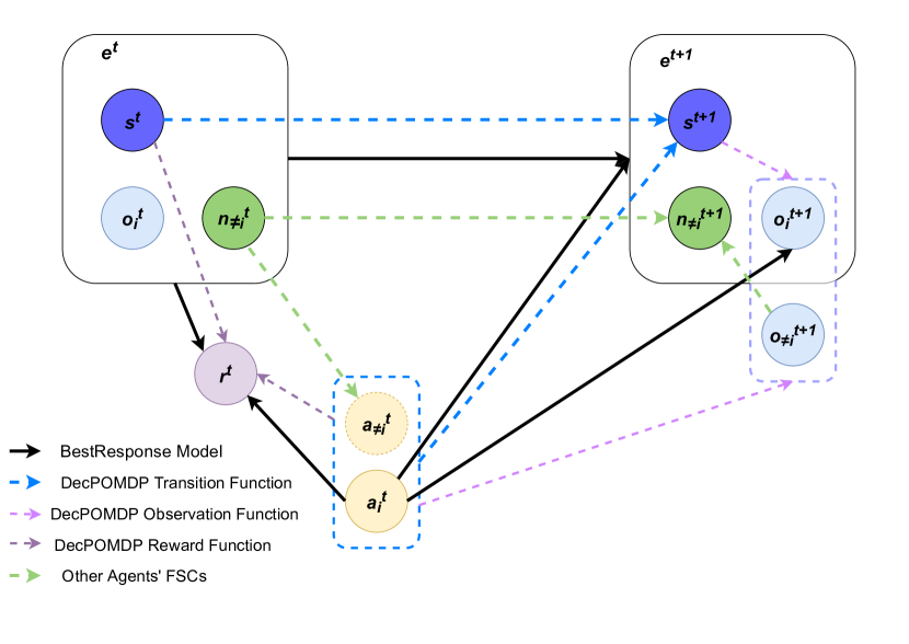
Figure 1: The decision-making structure for the best-response POMDP: The black arrows give a standard POMDP model; The purple dashed arrows show the transition function $T$ of the Dec-POMDP, i.e., the probability of next state $s^{t+1}$ given on current state $s^{t}$ and joint action $\langle a_{\neq i}^{t},a^{t}_{i}\rangle$; The blue dashed arrows show the observation function $O$ of the Dec-POMDP, i.e., the probability of joint observations $\langle o^{t+1}_{\neq i},o^{t+1}_{i}\rangle$ given the next state $s^{t+1}$ and joint action $\langle a_{\neq i}^{t},a^{t}_{i}\rangle$; The pink dashed arrows show the reward function; The green arrows show the evolution of agents $\neq i$’ FSC nodes.

This design choice for $e^{t}$ induces a POMDP because of the following properties: (i) it induces a Markov process controlled by the action (see dynamics below); (ii) the observation $o^{t}_{i}$ depends on $a^{t}_{i}$ and $e^{t+1}$; and (iii) the reward depends on $e^{t}$ and $a^{t}_{i}$. Indeed, deriving the transition, observation and reward functions for this POMDP (cf. App. A ) leads to:

$$T_{e}(e^{t},a^{t}_{i},e^{t+1})=Pr(e^{t+1}|e^{t},a^{t}_{i})$$

$$\quad=\sum_{o^{t+1}_{\neq i}}T(s^{t},\langle\psi_{\neq i}(n_{\neq i}^{t}),a^{t}_{i}\rangle,s^{t+1})\cdot\eta_{\neq i}(n_{\neq i}^{t},o^{t+1}_{\neq i},n_{\neq i}^{t+1})$$

$$\qquad\cdot O(s^{t+1},\langle\psi_{\neq i}(n_{\neq i}^{t}),a^{t}_{i}\rangle,\langle o^{t+1}_{\neq i},o^{t+1}_{i}\rangle),$$

$$O_{e}(a^{t}_{i},e^{t+1}_{i},o^{t+1}_{i})=Pr(o^{t+1}_{i}|a^{t}_{i},e^{t+1}_{i})$$

$$\quad=Pr(o^{t+1}_{i}|a^{t}_{i},\langle s^{t+1},n^{t+1}_{\neq i},\tilde{o}^{t+1}_{i}\rangle)=\mathbf{1}_{o^{t+1}_{i}=\tilde{o}^{t+1}_{i}},$$

$$r_{e}(e^{t},a^{t}_{i})=r(s^{t},a^{t}_{i},\psi_{\neq i}(n_{\neq i}^{t})),$$

where $\eta_{\neq i}(n_{\neq i}^{t},o^{t+1}_{\neq i},n_{\neq i}^{t+1})=\prod_{j\neq i}\eta(n_{j}^{t},\tilde{o}_{j}^{t+1},n_{j}^{t+1})$ and $\psi_{\neq i}(n_{\neq i}^{t})=a^{t}_{\neq i}$.

Note that the full observability of state variables such as $o^{t}_{i}$ can be exploited [21, 22], what we leave to the POMDP solver. Also, we make ${\cal E}$ smaller through state elimination, i.e., only keeping extended states reachable from the initial belief.

IV-C Obtaining and Evaluating $\mathit{fsc}_{i}$

Solve2FSC could rely on a solver that directly returns an FSC [19]. Instead, we choose to rely on a modern point-based approach (e.g., PBVI, HSVI or SARSOP [23, 24, 3]) returning an $\alpha$-vector set $\Gamma$ that approximates the optimal value function.

Algorithm

We use Algorithm 2, which is similar to Grześ et al.’s Alpha2FSC, to turn an $\alpha$-vector set $\Gamma$ into an FSC, where each node $n\stackrel{{\scriptstyle{\textrm{\rm\tiny def}}}}{{=}}\langle\alpha,a,b,w\rangle$ contains an $\alpha$-vector $\alpha$ with its (sometimes omitted) action $a$, and a representative belief $b$ (weighted average of the encountered beliefs mapped to this node) with its positive weight $w$ (which tries to capture the importance of this node). It first creates a start node $n_{0}$ from $b_{0}$ and $\Gamma$ with $w=1$ (line 2), and adds it to both the new FSC ($N$) and an open list ($G)$. Then, each $n$ in $G$ is processed (in fifo order) with each observation $o_{i}$ as follows ($0$-probability observations induce a self-loop (line 2)). Lines 2–2 compute the updated belief $b_{a_{i}}^{o_{i}}$, and the associated $w^{\prime}$ and $\alpha_{i}$. The node $n^{\prime}\in N$ that contains $\alpha_{i}$ is extracted if it exists and $b_{a_{i}}^{o_{i}}$ is merged into its representative belief (lines 2–2), otherwise a new node $n^{\prime}\stackrel{{\scriptstyle{\textrm{\rm\tiny def}}}}{{=}}\langle\alpha_{i},b_{a_{i}}^{o_{i}},w^{\prime}\rangle$ is created (line 2) and added to both $N$ and $G$. An edge $n\to n^{\prime}$, labeled with $o_{i}$, is then added (line 2).

As in Grześ et al.’s work, self-loops are added when an impossible observation $Pr(o_{i}|b,a_{i})=0$ is received. This may happen because, when building the FSC, each node $n_{i}$ is associated to a tuple $\langle\alpha_{i},b_{i}\rangle$, and outgoing edges from $n_{i}$ will be created only for observations that have non-zero probability in $b_{i}$. Yet, during execution $n_{i}$ may be reached while in a different belief $b^{\prime}$ from which $a_{i}$ (the action attached to $\alpha_{i}$, thus $n_{i}$) may induce “unexpected” observations. Adding self-loops is a way to equip the agent with a default strategy when such an unexpected observation occurs.

However, there are three differences in our method compared with Grześ et al.’s work: First, in [4], each input $\alpha$-vector comes with an associated beliefs, while we instead try to compute a belief representative of the reachable beliefs “attached” to the vector. Second, in [4], each $\alpha$-vector induces an FSC node ($|N|=|\Gamma|$), while we only consider $\alpha$-vectors reachable by the algorithm from $b_{0}$. Third, in our JESP setting, we have another reason for adding self-loops. Indeed, each agent $i$’s FSC is obtained considering fixed agent $\neq i$’s FSCs; yet, changing other agents’ FSCs will induce a new POMDP from $i$’s point of view, potentially with new possible observations when in certain nodes of $\mathit{fsc}_{i}$.

1

2

3[Input:] $\Gamma$: $\alpha$-vector set

4Start node $n_{0}\leftarrow node(\langle\operatorname*{arg\,max}_{\alpha\in\Gamma}(\alpha\cdot b_{0}),b_{0},1\rangle)$

5 $N\leftarrow\{n_{0}\}$

6 $G.pushback(n_{0})$

7 while $|G|>0$ do

8     $n\leftarrow G.popfront()$

9     $\langle b,a_{i},w\rangle\leftarrow\langle n.b,\psi(n),n.w\rangle$

10     forall $o_{i}\in\Omega_{i}$ do

11         if $Pr(o_{i}|b,a_{i})>0$  then

12             $b_{a_{i}}^{o_{i}}\leftarrow beliefUpdate(b,a_{i},o_{i})$

13             $w^{\prime}\leftarrow w\cdot Pr(o_{i}|b,a_{i})$

14             $\alpha_{i}\leftarrow argmax_{\alpha\in\Gamma}(\alpha\cdot b_{a_{i}}^{o_{i}})$

15             if $\alpha_{i}\notin N$  then

16                 $n^{\prime}\leftarrow node(\langle\alpha_{i},b_{a_{i}}^{o_{i}},w^{\prime}\rangle)$

17                 $N\leftarrow N\cup\{n^{\prime}\}$

18                 $G.pushback(n^{\prime})$

19                

20            else

21                 $n^{\prime}\leftarrow N(\alpha_{i})$

22                 $n^{\prime}.b\leftarrow\frac{n^{\prime}.w}{n^{\prime}.w+w^{\prime}}\cdot n^{\prime}.b+\frac{w^{\prime}}{n^{\prime}.w+w^{\prime}}\cdot b_{a_{i}}^{o_{i}}$

23                 $n^{\prime}.w\leftarrow n^{\prime}.w+w^{\prime}$

24            

25        else

26             $n^{\prime}\leftarrow n$

27            

28        $\eta(n,o_{i})\leftarrow n^{\prime}$

29        

30    

31

return $\langle N,\eta,\psi\rangle$

Algorithm 2 Extract FSC $\langle N,\eta,\psi\rangle$ from set $\Gamma$

Note that this algorithm does not bound the resulting number of internal nodes. Instead, we rely on (i) SARSOP returning finitely many $\alpha$-vectors, and (ii) the FSC extraction producing (significantly) less than $|\Gamma|$ internal nodes.

Once $\mathit{fsc}_{i}$ is obtained, the next step is to evaluate all agents’ policies in the Dec-POMDP. To that end, it is sufficient to evaluate $\mathit{fsc}_{i}$ in the corresponding best-response POMDP, since the latter combines in a single model the Dec-POMDP and the FSCs for agents $\neq i$. Here we used the FSC evaluation technique described in Sec. III-C.

IV-D MPOMDP Initializations

As previously mentioned, Inf-JESP’s initialization is important. Random initializations may often lead to poor local optima. Thus, we want to investigate if some non-random heuristic initializations allow to find good solutions quickly and reliably. Our method relies on solving an MPOMDP [5], i.e., assuming that observations are public. We extract individual FSCs from this MPOMDP policy as detailed below, and use them to initialize Inf-JESP.

MPOMDP-based Stochastic Initial FSC (M-S)

Algorithm 3 describes how to extract a policy $\mathit{fsc}_{i}$ for agent $i$ from an MPOMDP policy. This approach is similar to Algorithm 2, the main difference being that agent $\neq i$’s observations and actions should also be considered to compute a next belief. Yet, this is not actually feasible since agent $i$ is not aware of them. To address this issue, given agent $i$, let us consider a current node $n=\langle\alpha,b\rangle$ and an individual observation $o_{i}$ (i.e., with non-zero occurrence probability). The MPOMDP solution specifies a joint action $a=\langle a_{i},a_{\neq i}\rangle$ at $b$, $a_{i}$ being the action attached to $\alpha$. We arbitrarily assume that (i) each possible stochastic transition of the FSC (from $n$ and coming with observation $o_{i}$) corresponds to a possible joint observation $o_{\neq i}$ of the other agents, (ii) such a transition occurs with probability $Pr(o_{\neq i}\mid b,a,o_{i})$, and (iii) it “leads” to a new belief $b_{a}^{\langle o_{i},o_{\neq i}\rangle}$ and thus a node $n^{\prime}$ attached to the dominating MPOMDP $\alpha$-vector ($\alpha_{i}$, cf. line 3) at this point. As only one FSC node should correspond to a given $\alpha$-vector, a new $n^{\prime}$ attached to $\alpha_{i}$ is created only if necessary (lines 3, 3 and 3). As multiple joint observations $o_{\neq i}$ may lead to the same $n^{\prime}$, the corresponding transition probabilities are cumulated in $\eta(n,o_{i},n^{\prime})$ (line 3). $0$-probability joint observations $o_{\neq i}$ given $b$, $a$ and $o_{i}$ are ignored. $0$-probability individual observations $o_{i}$ given $b$ and $a$ induce the creation of a self-loop (line 3). Note that the resulting FSCs are stochastic, and some of them may never be improved on, so that, in this case, the solution returned by Inf-JESP may contain stochastic FSCs.

MPOMDP-based Deterministic Initial FSC (M-D)

A very simple variant of this method is to assume that the only possible transition from $n$ under $o_{i}$ corresponds to the most probable joint observation $o_{\neq i}$ of the other agents. Node transitions are then deterministic ($\eta(n,o_{i},n^{\prime})=1$).

Notes: (1) As both (i) these heuristic initializations and (ii) Inf-JESP’s local search are deterministic, using a deterministic procedure to derive best-response FSCs induces a deterministic algorithm for which restarts are useless. (2) These heuristic initializations can be also adapted to JESP’s finite-horizon setting by using policy trees.

1

2

3[Input:] $i$: agent $\mid$ $\Gamma$: MPOMDP $\alpha$-vector set

4Start node $n_{0}\leftarrow node(\langle argmax_{\alpha\in\Gamma}\alpha\cdot b_{0},b_{0},1\rangle)$

5 $N\leftarrow\{n_{0}\}$

6 $G.pushback(n_{0})$

7 while $|G|>0$ do

8     $n\leftarrow G.popfront()$

9     $\langle b,a,w\rangle\leftarrow\langle n.b,\psi(n),n.w\rangle$

10     forall  $o_{i}\in\Omega_{i}$  do

11         if $Pr(o_{i}|b,a)>0$ then

12             forall  $o_{\neq i}\in\Omega_{\neq i}$ do

13                 if $Pr(o_{\neq i}|o_{i},b,a)>0$  then

14                     $b_{a_{i}}^{\langle o_{i},o_{\neq i}\rangle}\leftarrow beliefUpdate(b,a_{i},\langle o_{i},o_{\neq i}\rangle)$

15                     $w^{\prime}\leftarrow w\cdot Pr(\langle o_{i},o_{\neq i}\rangle|b,a_{i})$

16                     $\alpha_{i}\leftarrow argmax_{\alpha}(b_{a}^{\langle o_{i},o_{\neq i}\rangle},\Gamma)$

17                     if $\alpha_{i}\notin N$  then

18                         $n^{\prime}\leftarrow node(\langle\alpha_{i},b_{a},w^{\prime}\rangle)$

19                         $N\leftarrow N\cup\{n^{\prime}\}$

20                         $G.pushback(n^{\prime})$

21                    else

22                         $n^{\prime}\leftarrow N(\alpha_{i})$

23                         $n^{\prime}.b\leftarrow\frac{n^{\prime}.w}{n^{\prime}.w+w^{\prime}}\cdot n^{\prime}.b+\frac{w^{\prime}}{n^{\prime}.w+w^{\prime}}\cdot b_{a_{i}}^{o_{i}}$

24                         $n^{\prime}.w\leftarrow n^{\prime}.w+w^{\prime}$

25                    $\eta(n,o_{i},n^{\prime})\leftarrow\eta(n,o_{i},n^{\prime})+Pr(o_{\neq i}|o_{i},b,a)$

26                

27            

28        else

29             $\eta(n,o_{i},n)\leftarrow 1$

30        

31    

return $\langle N,\eta,\psi\rangle$

Algorithm 3 Extract $FSC_{i}$ from MPOMDP set $\Gamma$

V Experiments

In this section, we evaluate variants of Inf-JESP and other state-of-the-art solvers on various Dec-POMDP benchmarks.

V-A Comparison method

The standard Dec-POMDP benchmark problems we use are: DecTiger, Recycling, Meeting in a 3$\times$3 grid, Box Pushing, and Mars Rover (cf. http://masplan.org/problem).

We compare the different variants of Inf-JESP with state-of-the-art Dec-POMDP algorithms, namely: FB-HSVI [7], Peri [13], PeriEM [13], PBVI-BB [8] and MealyNLP [10]. We ignore JESP as it only handles finite horizons. Dec-BPI is compared separately because we can only estimate values from empirical graphs on some benchmark problems [18].

V-B Algorithm settings

SARSOP [3] is our POMDP solver, with a $0.001$ Bellman residual (also for FSC evaluation) and a $5$ s timeout.

We have tested 4 variants of Inf-JESP. IJ(M-D) and IJ(M-S) are Inf-JESP initialized with the M-D and M-S heuristics (Sec. IV-D) and without restarts (because they behave deterministically). IJ(R-$1$) and IJ(R-$100$) are Inf-JESP with random initializations (at most 5 nodes per FSC) and, respectively, 1 (re)start and 100 restarts. Each restart has a timeout of $7200$ s. Due to the limited time, we did not perform random restart tests on the Box-Pushing and Mars Rover domains. IJ(R-$x_{y}$) denotes $y$ runs of IJ(R-$x$) used to compute statistics.

The experiments with Inf-JESP were conducted on a laptop with an i5-1.6 GHz CPU and 8 GB RAM. The source code is available at https://gitlab.inria.fr/ANR_FCW/InfJESP .

V-C Results

V-C1 Comparison with state-of-the-art algorithms

Table I: Comparison of different algorithms in terms of final FSC size, number of iterations, time and value, on five infinite-horizon benchmark problems with $\gamma=0.9$ for all domains.
R-$R_{N}$ = $N$ runs with $R$ random restarts each. M-S and M-D = deterministic initializations with stochastic extracted FSCs and deterministic extracted FSCs from a MPOMDP solution.

Alg.	FSC size	#Iterations	Time (s)	Value
DecTiger ($|{\cal I}|=2,|{\cal S}|=2,|{\cal A}^{i}|=3,|{\cal Z}^{i}|=2$)
FB-HSVI			$153.7$	$13.448$
PBVI-BB				$13.448$
Peri			$220$	$13.45$
IJ(R-$100_{5}$)	$9{\scriptstyle\pm 3}\times 8{\scriptstyle\pm 4}$	$33$$\!\!{\scriptstyle\pm 1}$	$12\,417.6$	$13.44$
IJ(M-D)	$6\times 6$	$36$	$201$	$13.44$
IJ(M-S)	$6\times 6$	$27$	$213$	$13.44$
PeriEM			$6450$	$9.42$
MealyNLP			$29$	$-1.49$
IJ(R-$1_{500}$)	$29{\scriptstyle\pm 55}\times 32{\scriptstyle\pm 54}$	$21$$\!\!{\scriptstyle\pm 14}$	$124.18$	$-35.47$
Recycling ($|{\cal I}|=2,|{\cal S}|=4,|{\cal A}^{i}|=3,|{\cal Z}^{i}|=2$)
FB-HSVI			$2.6$	$31.929$
PBVI-BB				$31.929$
MealyNLP			$0$	$31.928$
Peri			$77$	$31.84$
PeriEM			$272$	$31.80$
IJ(R-$100_{10}$)	$2{\scriptstyle\pm 0}\times 2{\scriptstyle\pm 0}$	$3$$\!\!{\scriptstyle\pm 0}$	$3.1$	$31.62$
IJ(R-$1_{1000}$)	$3{\scriptstyle\pm 2}\times 3{\scriptstyle\pm 2}$	$3$$\!\!{\scriptstyle\pm 0}$	$0.03$	$30.60$
IJ(M-S)	$8\times 8$	$3$	$0$	$26.57$
IJ(M-D)	$4\times 4$	$3$	$0$	$25.65$
Grid3*3 ($|{\cal I}|=2,|{\cal S}|=81,|{\cal A}^{i}|=5,|{\cal Z}^{i}|=9$)
IJ(M-D)	$8\times 10$	$3$	$2$	$5.81$
IJ(M-S)	$9\times 17$	$3$	$9$	$5.81$
IJ(R-$100_{5}$)	$\ 13{\scriptstyle\pm 6}\times 9{\scriptstyle\pm 0}$	$4$$\!\!{\scriptstyle\pm 0}$	$413.8$	$5.81$
FB-HSVI			$67$	$5.802$
IJ(R-$1_{500}$)	$11{\scriptstyle\pm 18}\times 11{\scriptstyle\pm 18}$	$3$$\!\!{\scriptstyle\pm 1}$	$4.14$	$5.79$
Peri			$9714$	$4.64$
Box-pushing ($|{\cal I}|=2,|{\cal S}|=100,|{\cal A}^{i}|=4,|{\cal Z}^{i}|=5$)
FB-HSVI			$1715.1$	$224.43$
PBVI-BB				$224.12$
IJ(M-S)	$250\times 408$	$6$	$963$	$220.25$
IJ(M-D)	$\ 274\times 342$	$8$	$1436$	$203.41$
Peri			$5675$	$148.65$
MealyNLP			$774$	$143.14$
PeriEM			$7164$	$106.65$
Mars Rover ($|{\cal I}|=2,|{\cal S}|=256,|{\cal A}^{i}|=6,|{\cal Z}^{i}|=8$)
FB-HSVI			$74.31$	$26.94$
IJ(M-D)	$125\times 183$	$6$	$122$	$26.91$
IJ(M-S)	$84\times 64$	$5$	$66$	$24.17$
Peri			$6088$	$24.13$
MealyNLP			$396$	$19.67$
PeriEM			$7132$	$18.13$

Table I presents the results for the 5 problems. For IJ(R-$x_{y}$), in each run we kept the highest value among the restarts, and then computed the average of this value over the various runs. The columns provide: (Alg.) the different algorithms at hand, (N) the final FSCs’ sizes (for Inf-JESPs), (I) the number of iterations required to converge (for Inf-JESPs), (Time) the running time, (Value) the final value (lower bounds for Inf-JESPs, the true value being at most 0.01 higher).

In terms of final value achieved, Inf-JESP variants find good to very good solutions in most cases, often very close to FB-HSVI’s near-optimal solutions. Comparing with estimated values obtained by Dec-BPI on the DecTiger, Grid and Box-Pushing problems (using the figures in [18, p. 123]), Inf-JESP outperforms Dec-BPI in these three problems. Note also that Dec-BPI’s results highly depend on the size of the considered FSCs and that Dec-BPI faces difficulties with large FSCs, e.g., in the DecTiger problem [18].

Regarding the solving time, Inf-JESP variants have different behaviors depending on the problem at hand. For example, in DecTiger, IJ(M-S) and IJ(M-D) have almost the same solving time, and both of them require more time than IJ(R-$1_{500}$). However, in other problems, IJ(M-D) and IJ(M-S) may require very different solving times. Overall, IJ(M-D) and IJ(M-S) can give good solutions within an acceptable amount of time.

V-C2 Study of Inf-JESP

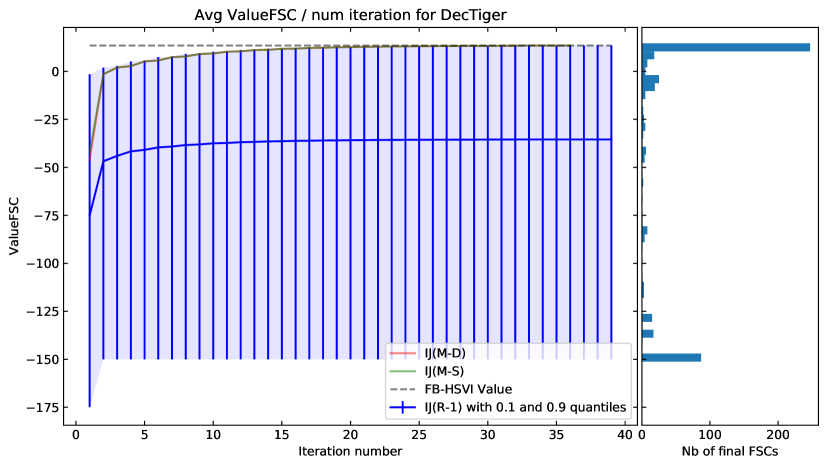
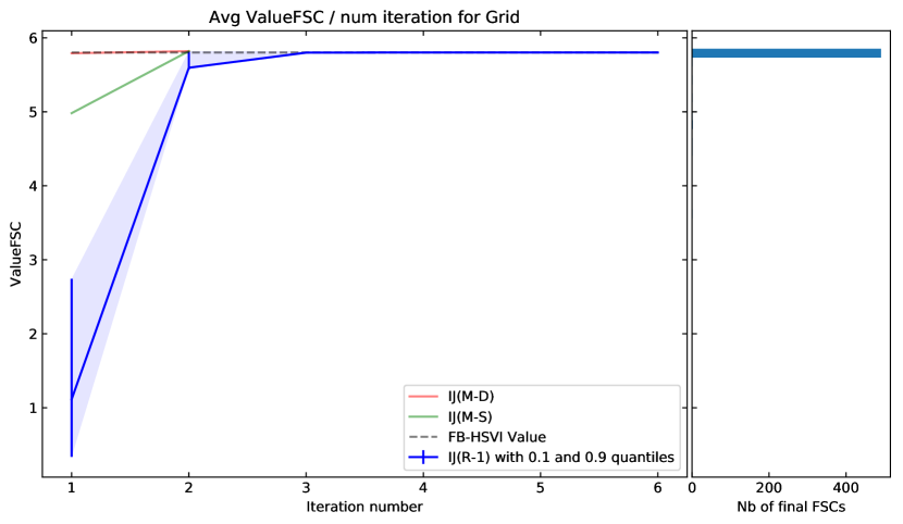
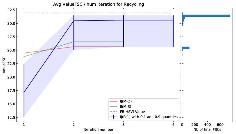
Figure 2: Values of the joint policy for the DecTiger, Grid and Recycling problems (from top to bottom). The left part of each figure presents the evolution (during a run) of the value of the joint policy at each iteration of: IJ(R-$1$) (avg + 10th and 90th percentiles in blue), and the deterministic IJ(M-D) (in red) and IJ(M-S) (in green). The dashed line represents FB-HSVI’s final value. The right part presents the value distribution after convergence of IJ(R-$1$).

Fig. 2 (right) presents the distribution over final values of IJ(R-$1$). In the three problems at hand, most runs end with (near-) globally optimal values, despite initial FSCs limited to 5 nodes. Other local optima turn out to be rarely obtained, except in DecTiger. These distributions show that few restarts are needed to reach a global optimum with high probability.

Fig. 2 (left) presents the evolution of the FSC values during a JESP run as a function of the iteration number for IJ(R-$1$) (avg + 10th and 90th percentiles in blue), IJ(M-D) (in green) and IJ(M-S) (in red). For random initialization, at each iteration the average is computed over all runs, even if they have already converged. This figure first shows that (i) Inf-JESP’s solution quality monotonically increases during a run, and (ii) most runs converge to local optima in few iterations. It also illustrates that MPOMDP initializations are rather good heuristics compared to random ones but, as expected, do not always lead to a global optimum (cf. the Recycling problem).

V-C3 Complementary results

The experiments also showed (cf. detailed results in App. B) that IJ(R-$1$) exhibits different behaviors depending on the problem at hand. For instance, removing unreachable extended states (Sec. IV-B) divides their number on average by 1 in DecTiger (which is expected since, in this case, any observation can be received from any state), 50 in Grid3*3, and 5 in Recycling. We also observed that final FSCs with the highest values are not obtained with the more iterations and do not contain the more nodes. Small FSCs seem sufficient to obtain good solutions, opening an interesting research direction to combine Inf-JESP with FSC compression.

VI Conclusion

We proposed a new infinite-horizon Dec-POMDP solver, Inf-JESP, which is based on JESP, but using FSC representations for policies instead of trees. FSCs allow not only to handle infinite horizons, but also to possibly derive compact policies. Any restart of the ideal algorithm provably converges to a Nash optimum, and, despite the existence of local optima, experiments show frequent convergence close to global optima in five standard benchmark problems. One ingredient, the derivation of a POMDP from $|{\cal I}|-1$ fixed FSCs, could also be useful in other settings where other agents’ behaviors are defined independently, as games [25] or Human-Robot interactions [26].

We also provided a method to extract individual policies (FSCs) from an MPOMDP solution $\alpha$-vector set $\Gamma$ to initialize Inf-JESP. This approach can be easily adapted to JESP for the finite-horizon setting. Empirical results showed that this initialization method could, in some cases, reach good solutions with a value higher than the average answer of Inf-JESP with random initialization. However, this approach does not always work. In the Recycling problem, it is worse than the average Inf-JESP value with random initializations. How to derive (possibly randomly) better heuristic initializations from MPOMDP policies remains an open question.

Future work includes experimenting with (i) bounded FSC sizes (to enforce compactness of policies); (ii) different best-response POMDP formalizations; (iii) different timeouts for SARSOP; (iv) parallelized restarts.

Appendix A Notes about the Candidate POMDP Formalizations

We here look in more details at how, given the Dec-POMDP and FSCs for all agents but $i$, one can derive a valid best-response POMDP from agent $i$’s point of view. First, note that, in the POMDP formalization:

• we have no choice for the observation ($o^{t}_{i}$) and for the action ($a^{t}_{i}$), which are pre-requisites;

• the only choice that can be made is that of the variables put in the (extended) state $e^{t}_{i}$;

• the transition, observation and reward functions are consequences of this choice.

Also, note that, in a POMDP formalization, the state and observation variables need be distinguished. One cannot write that $X$ is an observed state variable (contrary to the MOMDP formalism). In the following, it is thus important to distinguish the different types of random variables. In particular,

• $O^{t}_{i}$ always denotes (of course) the observation variable, yet

• $\tilde{O}^{t}_{i}$ denotes either an intermediate variable or a state variable (which, in both cases, is strongly dependent on observation variable $O^{i}_{t}$ since their values are always equal).

The main issue when designing our BR POMDP is to verify that the dependencies in the transition, observation, and reward functions are the appropriate ones (see Fig. 3 (top left)). In the following paragraphs, we consider 3 choices for the extended state of the POMDP, check whether they indeed induce valid POMDPs, and derive the induced transition, observation and reward functions when appropriate.

$e^{t}=\langle s^{t},n^{t}_{\neq i}\rangle$ ?

To show that $e^{t}=\langle s^{t},n^{t}_{\neq i}\rangle$ does not induce a proper POMDP, let us write the transition function:

$$T_{e}(e^{t},a^{t}_{i},e^{t+1})\stackrel{{\scriptstyle{\textrm{\rm\tiny def}}}}{{=}}Pr(e^{t+1}|e^{t},a^{t}_{i})$$

$$=Pr(s^{t+1},n_{\neq i}^{t+1}|s^{t},n_{\neq i}^{t},a^{t}_{i})$$

$$=\sum_{\tilde{o}^{t+1}}Pr(s^{t+1},n_{\neq i}^{t+1},\tilde{o}^{t+1}|s^{t},n_{\neq i}^{t},a^{t}_{i})$$

$$=\sum_{\tilde{o}^{t+1}}Pr(n_{\neq i}^{t+1}|s^{t},n_{\neq i}^{t},a^{t}_{i},s^{t+1},\tilde{o}^{t+1})$$

$$\quad\cdot Pr(s^{t+1},\tilde{o}^{t+1}|s^{t},n_{\neq i}^{t},a^{t}_{i})$$

$$=\sum_{\tilde{o}^{t+1}}Pr(n_{\neq i}^{t+1}|s^{t},n_{\neq i}^{t},a^{t}_{i},s^{t+1},\tilde{o}^{t+1})$$

$$\quad\cdot Pr(\tilde{o}^{t+1}|s^{t},n_{\neq i}^{t},a^{t}_{i},s^{t+1})\cdot Pr(s^{t+1}|s^{t},n_{\neq i}^{t},a^{t}_{i})$$

$$=\sum_{\tilde{o}^{t+1}}\left(\prod_{j\neq i}\eta(n_{j}^{t},\tilde{o}_{j}^{t+1},n_{j}^{t+1})\right)$$

$$\cdot O(\langle\psi_{\neq i}(n_{\neq i}^{t}),a^{t}_{i}\rangle,s^{t+1},\tilde{o}^{t+1})\cdot T(s^{t},\langle\psi_{\neq i}(n_{\neq i}^{t}),a^{t}_{i}\rangle,s^{t+1}),$$

where $\tilde{O}^{t+1}$ is a temporary variable, not a state or an observation variable. Here, as illustrated by Fig. 3 (top right), the issue is that the actual observation variable $O_{i}^{t+1}$ is not independent on $E^{t}$ given $E^{t+1}$ and $A^{t}$.

$e^{t}=\langle s^{t},n^{t}_{\neq i},\tilde{o}^{t}_{i}\rangle$ ?

We correct the first attempt by adding a state variable $\tilde{O}^{t}_{i}$, thus defining $e^{t}=\langle s^{t},n^{t}_{\neq i},\tilde{o}^{t}_{i}\rangle$, hence:

$$T_{e}(e^{t},a^{t}_{i},e^{t+1})\stackrel{{\scriptstyle{\textrm{\rm\tiny def}}}}{{=}}Pr(e^{t+1}|e^{t},a^{t}_{i})$$

$$=Pr(s^{t+1},n_{\neq i}^{t+1},\tilde{o}_{i}^{t+1}|s^{t},n_{\neq i}^{t},\tilde{o}_{i}^{t},a^{t}_{i})$$

$$=\sum_{o^{t+1}_{\neq i}}Pr(s^{t+1},n_{\neq i}^{t+1},o^{t+1}_{i-1},\tilde{o}_{i}^{t}|s^{t},n_{\neq i}^{t},\tilde{o}_{i}^{t},a^{t}_{i})$$

$$=\sum_{o^{t+1}_{\neq i}}Pr(n_{\neq i}^{t+1}|s^{t},n_{\neq i}^{t},\tilde{o}_{i}^{t},a^{t}_{i},s^{t+1},o^{t+1})$$

$$\quad\cdot Pr(s^{t+1},o^{t+1}_{\neq i},\tilde{o}_{i}^{t+1}|s^{t},n_{\neq i}^{t},\tilde{o}_{i}^{t},a^{t}_{i})$$

$$=\sum_{o^{t+1}_{\neq i}}Pr(n_{\neq i}^{t+1}|s^{t},n_{\neq i}^{t},\tilde{o}_{i}^{t},a^{t}_{i},s^{t+1},o^{t+1})$$

$$\cdot Pr(o^{t+1}_{\neq i},\tilde{o}_{i}^{t+1}|s^{t},n_{\neq i}^{t},\tilde{o}_{i}^{t},a^{t}_{i},s^{t+1})\cdot Pr(s^{t+1}|s^{t},n_{\neq i}^{t},\tilde{o}_{i}^{t},a^{t}_{i})$$

$$=\sum_{o^{t+1}_{\neq i}}\Big{(}\prod_{j\neq i}\eta(n_{j}^{t},o_{j}^{t+1},n_{j}^{t+1})\Big{)}$$

$$\cdot O(\langle\psi_{\neq i}(n_{\neq i}^{t}),a^{t}_{i}\rangle,s^{t+1},o^{t+1})\cdot T(s^{t},\langle\psi_{\neq i}(n_{\neq i}^{t}),a^{t}_{i}\rangle,s^{t+1}).$$

The formula above does not raise the same issue as $$\tilde{O}^{t}_{i} O^{t}_{i}$$ is a state variable, and the observation variable now does not depend on the previous state given the new one and the action (cf. Fig. 3 (bottom right)). Also, we have the following observation function:

$$O_{e}(a^{t}_{i},e^{t+1}_{i},o^{t+1}_{i})\stackrel{{\scriptstyle{\textrm{\rm\tiny def}}}}{{=}}Pr(o^{t+1}_{i}|a^{t}_{i},e^{t+1}_{i})$$

$$=Pr(o^{t+1}_{i}|a^{t}_{i},\langle s^{t+1},n^{t+1}_{\neq i},\tilde{o}^{t+1}_{i}\rangle)=\mathbf{1}_{o^{t+1}_{i}=\tilde{o}^{t+1}_{i}},$$

and the trivial reward function:

$$r_{e}(e^{t},a^{t}_{i})=r(s^{t},a^{t}_{i},\psi_{\neq i}(n_{\neq i}^{t})).$$

$e^{t}=\langle s^{t},n^{t-1}_{\neq i},\tilde{o}^{t}_{\neq i}\rangle$ ?

In this work, we have also considered a third choice for the extended state, defined as $e^{t}=\langle s^{t},n^{t-1}_{\neq i},\tilde{o}^{t}_{\neq i}\rangle$, where $\tilde{O}^{t}_{\neq i}$ is a state variable (not an observation variable) corresponding to other agents’ observations at time $t$:

$$T_{e}(e^{t},a^{t}_{i},e^{t+1})\stackrel{{\scriptstyle{\textrm{\rm\tiny def}}}}{{=}}Pr(e^{t+1}|e^{t},a^{t}_{i})$$

$$=Pr(s^{t+1},n_{\neq i}^{t},\tilde{o}_{\neq i}^{t+1}|s^{t},n_{\neq i}^{t-1},\tilde{o}_{\neq i}^{t},a^{t}_{i})$$

$$=Pr(\tilde{o}_{\neq i}^{t+1}|s^{t+1},n_{\neq i}^{t},s^{t},n_{\neq i}^{t-1},\tilde{o}_{\neq i}^{t},a^{t}_{i})$$

$$\quad\cdot Pr(s^{t+1},n_{\neq i}^{t}|s^{t},n_{\neq i}^{t-1},\tilde{o}_{\neq i}^{t},a^{t}_{i})$$

$$=Pr(\tilde{o}_{\neq i}^{t+1}|s^{t+1},n_{\neq i}^{t},s^{t},n_{\neq i}^{t-1},\tilde{o}_{\neq i}^{t},a^{t}_{i})$$

$$\quad\cdot Pr(s^{t+1}|n_{\neq i}^{t},s^{t},n_{\neq i}^{t-1},\tilde{o}_{\neq i}^{t},a^{t}_{i})$$

$$\quad\cdot Pr(n_{\neq i}^{t}|s^{t},n_{\neq i}^{t-1},\tilde{o}_{\neq i}^{t},a^{t}_{i})$$

$$=Pr(s^{t+1}|s^{t},n_{\neq i}^{t},a^{t}_{i})\cdot Pr(n_{\neq i}^{t}|n_{\neq i}^{t-1},\tilde{o}_{\neq i}^{t})$$

$$\quad\cdot Pr(\tilde{o}_{\neq i}^{t+1}|s^{t+1},n_{\neq i}^{t},a^{t}_{i})$$

$$=Pr(s^{t+1}|s^{t},n_{\neq i}^{t},a^{t}_{i})\cdot Pr(n_{\neq i}^{t}|n_{\neq i}^{t-1},\tilde{o}_{\neq i}^{t})$$

$$\quad\cdot\sum_{\tilde{o}^{t+1}_{i}}Pr(\tilde{o}_{\neq i}^{t+1},\tilde{o}^{t+1}_{i}|s^{t+1},n_{\neq i}^{t},a^{t}_{i})$$

$$=T(s^{t},\langle\psi_{\neq i}(n_{\neq i}^{t}),a^{t}_{i}\rangle,s^{t+1})\cdot\prod_{j\neq i}\eta(n_{j}^{t-1},o_{j}^{t},n_{j}^{t})$$

$$\quad\cdot\sum_{\tilde{o}^{t+1}_{i}}O(\langle\psi_{\neq i}(n_{\neq i}^{t}),a^{t}_{i}\rangle,s^{t+1},\langle\tilde{o}_{\neq i}^{t+1},\tilde{o}^{t+1}_{i}\rangle).$$

The formula above does not raise issues. As illustrated by Fig. 3 (bottom right), the actual observation variable $$O_{i}^{t+1} E^{t} E^{t+1} A^{t}$$ is independent on given and . Also, we have the following observation function:

$$O_{e}(a^{t}_{i},e^{t+1}_{i},o^{t+1}_{i})\stackrel{{\scriptstyle{\textrm{\rm\tiny def}}}}{{=}}Pr(o^{t+1}_{i}|a^{t}_{i},e^{t+1}_{i})$$

$$=Pr(o^{t+1}_{i}|a^{t}_{i},\langle s^{t+1},n^{t}_{\neq i},\tilde{o}^{t+1}_{\neq i}\rangle)$$

$$=\frac{Pr(\tilde{o}^{t+1}_{\neq i},o^{t+1}_{i},s^{t+1},n^{t}_{\neq i},a^{t}_{i})}{Pr(\tilde{o}^{t+1}_{\neq i},s^{t+1},n^{t}_{\neq i},a^{t}_{i})}$$

$$=\frac{Pr(\tilde{o}^{t+1}_{\neq i},o^{t+1}_{i}|s^{t+1},n^{t}_{\neq i},a^{t}_{i})}{\sum_{o^{t+1}_{i}}Pr(\tilde{o}^{t+1}_{\neq i},o^{t+1}_{i}|s^{t+1}n^{t}_{\neq i},a^{t}_{i})}$$

$$=\frac{O(\langle\psi_{\neq i}(n_{\neq i}^{t}),a^{t}_{i}\rangle,s^{t+1},\langle\tilde{o}_{\neq i}^{t+1},o^{t+1}_{i}\rangle)}{\sum_{\tilde{o}^{t+1}_{i}}O(\langle\psi_{\neq i}(n_{\neq i}^{t}),a^{t}_{i}\rangle,s^{t+1},\langle\tilde{o}_{\neq i}^{t+1},\tilde{o}^{t+1}_{i}\rangle)}.$$

We can see that the denominator is identical to the last part of the transition function. In practice, when computing transition probabilities, we will store the values for $$\sum_{\tilde{o}^{t+1}_{i}}O(\langle\psi_{\neq i}(n_{\neq i}^{t}),a^{t}_{i}\rangle,s^{t+1},\langle\tilde{o}_{\neq i}^{t+1},\tilde{o}^{t+1}_{i}\rangle)$$ so as to reuse them when computing the observation function. In the end, the reward function is obtained with:

$$r_{e}(e^{t},a^{t}_{i})=r(\langle s^{t},n^{t-1}_{\neq i},\tilde{o}^{t}_{\neq i}\rangle,a^{t}_{i})$$

$$=\sum_{n^{t}_{\neq i}}Pr(n^{t}_{\neq i}|n^{t-1}_{\neq i},\tilde{o}^{t}_{\neq i})\cdot r(s^{t},n^{t-1}_{\neq i},a^{t}_{i})$$

$$=\sum_{n^{t}_{\neq i}}\Big{(}\prod_{j\neq i}\eta(n_{j}^{t-1},\tilde{o}_{j}^{t},n_{j}^{t})\Big{)}\cdot r(s^{t},\langle\psi_{\neq i}(n_{\neq i}^{t}),a^{t}_{i}\rangle).$$

Different formalizations lead to different state spaces with different sizes, so that the time and space complexities of the generation of this best-response POMDP or of its solving will depend on the choice of formalization. Which choice is best shall depend on the Dec-POMDP at hand, and possibly on the current FSCs. We have opted for the simplest of the two formalizations presented above (which we call the “MOMDP formalization” because one state variable is fully observed), but observed little differences in practice in our experiments.

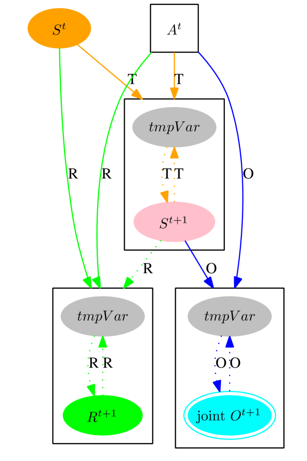
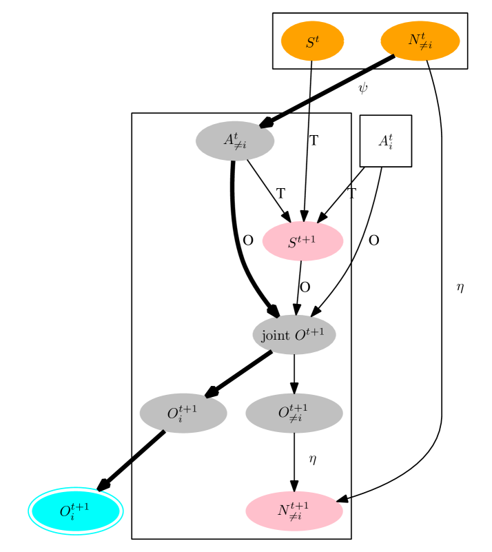
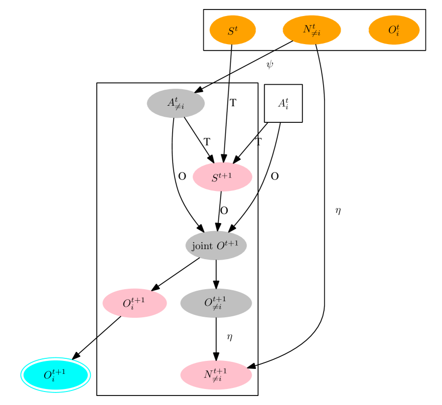
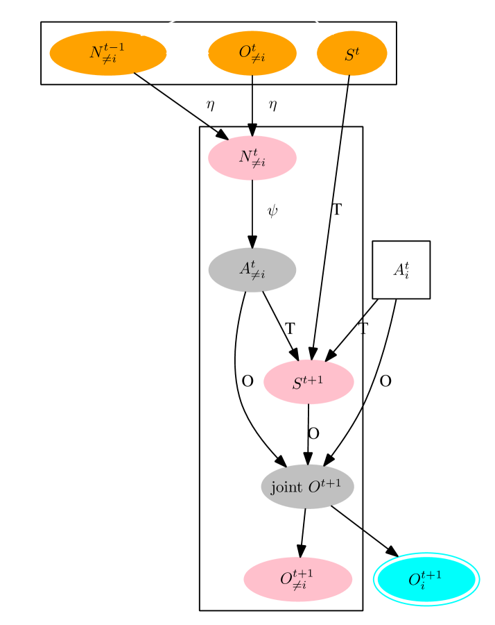
Figure 3: (top left) Standard POMDP dependencies, including intermediate variables used to compute the transition function (only); and candidate Best-Response POMDP formalizations with: (top right) $e^{t}_{i}\stackrel{{\scriptstyle{\textrm{\rm\tiny def}}}}{{=}}\langle s^{t},n^{t}_{\neq i}\rangle$, (bottom left) $e^{t}_{i}\stackrel{{\scriptstyle{\textrm{\rm\tiny def}}}}{{=}}\langle s^{t},n^{t}_{\neq i},o^{t}_{i}\rangle$, and (bottom right) $e^{t}_{i}\stackrel{{\scriptstyle{\textrm{\rm\tiny def}}}}{{=}}\langle s^{t},n^{t-1}_{\neq i},o^{t}_{\neq i}\rangle$.

Appendix B Supplementary Figures

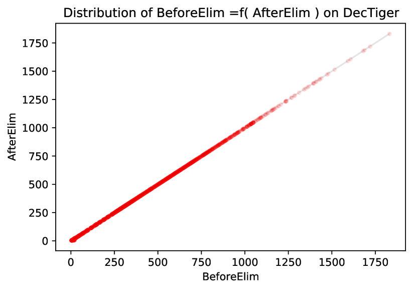
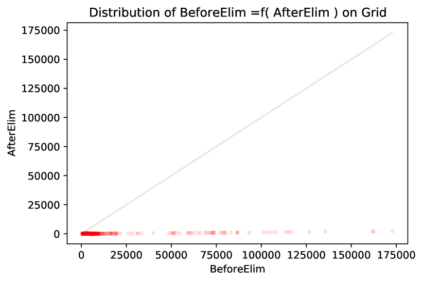
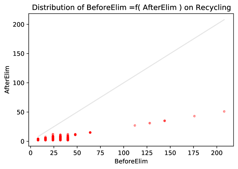
Figure 4: Effect of the state elimination for the DecTiger, Grid and Recycling problems (from left to right). Each figure plots, for each Best-Response POMDP obtained while executing Inf-JESP(R-$1_{1}$), the number of states of that POMDP after state elimination as a function of that number before state elimination.

Regarding state elimination (as explained in Section IV-B), it turned out that, for the “MOMDP” best-response POMDP, the ratio of the initial number of (extended) states over its number of states after state elimination depends on the problem at hand but does not depend on the Inf-JESP run (see Figure 4). This ratio was 1 for the DecTiger problem, 50 for the Grid problem, and 5 for the Recycling problem. These differences are due to the stochasticity of the observation process, which limits or even prevents state elimination. As it is currently done, state elimination is based on the probability of generating a specific observation from a state considering possible actions. However, for the DecTiger problem, every observation can be generated whatever the considered action, leading to no state elimination (contrary to the Grid and the Recycling problem).

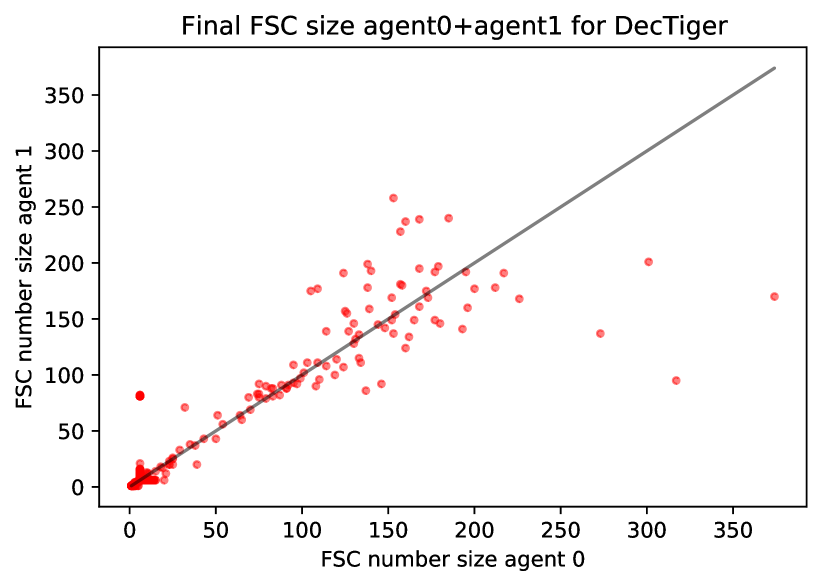
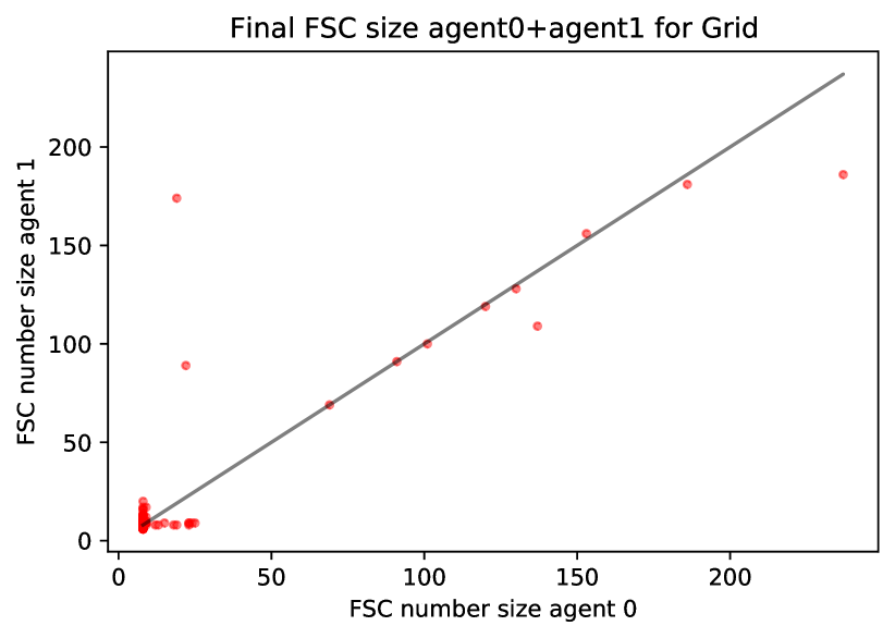
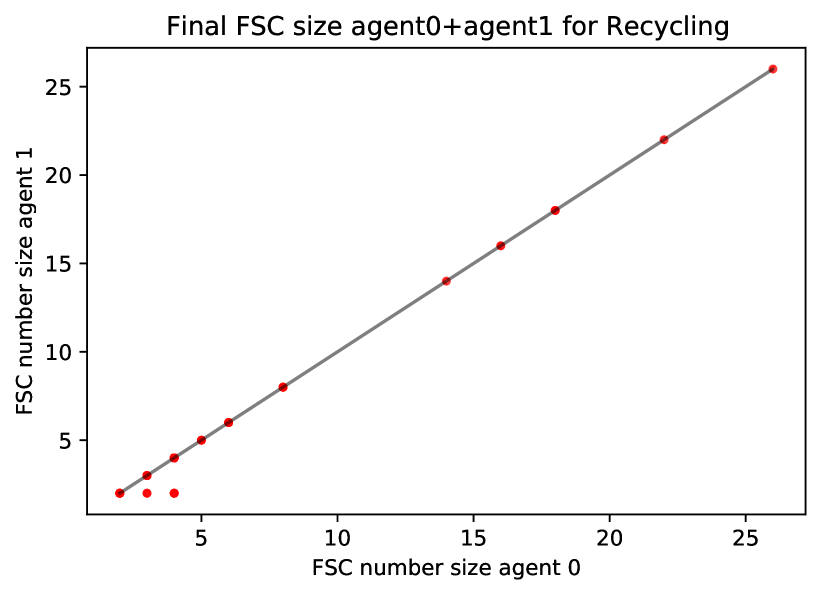
Figure 5: Sizes of the final FSCs obtained with Inf-JESP(R-$1_{1}$) after convergence for the DecTiger, Grid and Recycling problems (from left to right). Each dot corresponds to a pair containing the sizes of both agents’ FSCs.

Regarding the size of the final FSCs obtained after convergence of an Inf-JESP run with a random initialization (see Figure 5), we also observed different behaviors. Applied to the DecTiger problem, Inf-JESP leads to a very large distribution of the sizes of the final FSCs. Applied to the Recycling problem, Inf-JESP also leads to a large distribution of the sizes of the final FSC, but the sizes of the FSCs of both agents are symmetrical. Applied to the Grid problem, Inf-JESP generates a large number of FSC pairs of size 10 with sometimes huge variation and with a tendency to be asymmetrical, the first optimized agent having a tendency to have more FSC nodes. These results need to be further investigated in order to understand them clearly and see if it is possible to link them to the nature of the addressed domain.

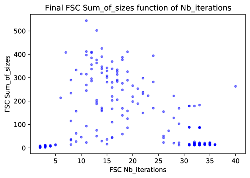
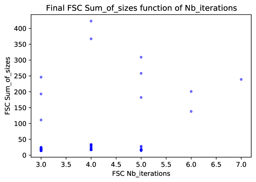
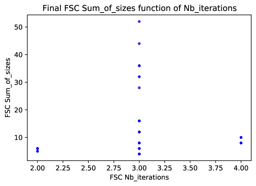
Figure 6: Sum of the sizes of the final FSCs obtained with Inf-JESP(R-$1_{1}$) after convergence as a function of the required number of iterations for the DecTiger, Grid and Recycling problems (from left to right).

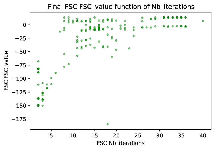
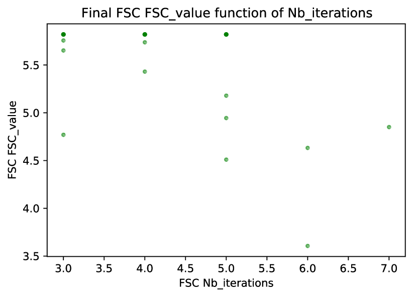
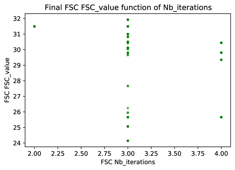
Figure 7: Value of the final FSCs obtained with Inf-JESP(R-$1_{1}$) after convergence as a function of the required number of iterations for the DecTiger, Grid and Recycling problems (from left to right).

It must also be noted that the sizes of the FSCs do not monotonically increase during one Inf-JESP iteration (data not presented here). Sometimes the size of the FSC computed during one Inf-JESP improvement decreases, meaning that the solution to the best-response POMDP is a FSC with a smaller size but a higher value (as commonly observed in the DecTiger problem). When looking at the FSCs obtained at the end of one Inf-JESP run, another observed phenomenon is that the more iterations required to reach the equilibrium, the smaller the sizes of the final FSCs (see Figure 6). But this does not mean that the associated value is higher (see Figure 7).

Finally, Figure 8 presents the values of the obtained equilibria as a function of the sum of sizes of the FSCs obtained by Inf-JESP(R-$1_{1}$) after convergence. It can be observed that small FSCs seem to be sufficient to generate a high value, opening new directions on combining Inf-JESP with FSC compression.

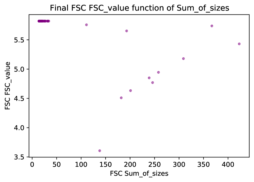
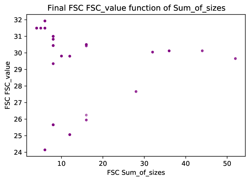
Figure 8: Value of the final FSCs obtained with Inf-JESP(R-$1_{1}$) after convergence as a function of the sum of the sizes of final FSCs for the DecTiger, Grid and Recycling problems (from left to right).

References

- Bernstein et al. [2002] D. Bernstein, R. Givan, N. Immerman, and S. Zilberstein, “The complexity of decentralized control of Markov decision processes,” Math. of Operations Research, vol. 27, no. 4, 2002.
- Nair et al. [2003] R. Nair, M. Tambe, M. Yokoo, D. Pynadath, and S. Marsella, “Taming decentralized POMDPs: Towards efficient policy computation for multiagent settings,” in IJCAI, 2003.
- Kurniawati et al. [2008] H. Kurniawati, D. Hsu, and W. Lee, “SARSOP: Efficient point-based POMDP planning by approximating optimally reachable belief spaces,” in RSS, 2008.
- Grześ et al. [2015] M. Grześ, P. Poupart, X. Yang, and J. Hoey, “Energy efficient execution of POMDP policies,” IEEE Trans. on Cybernetics, vol. 45, 2015.
- Pynadath and Tambe [2002] D. V. Pynadath and M. Tambe, “The communicative multiagent team decision problem: Analyzing teamwork theories and models,” JAIR, vol. 16, Jun 2002.
- Szer et al. [2005] D. Szer, F. Charpillet, and S. Zilberstein, “MAA*: A heuristic search algorithm for solving decentralized POMDPs,” in UAI, 2005.
- Dibangoye et al. [2016] J. Dibangoye, C. Amato, O. Buffet, and F. Charpillet, “Optimally solving Dec-POMDPs as continuous-state MDPs,” JAIR, vol. 55, 2016.
- MacDermed and Isbell [2013] L. C. MacDermed and C. Isbell, “Point based value iteration with optimal belief compression for Dec-POMDPs,” in NIPS, 2013.
- Amato et al. [2010a] C. Amato, D. S. Bernstein, and S. Zilberstein, “Optimizing fixed-size stochastic controllers for POMDPs and decentralized POMDPs,” JAAMAS, vol. 21, no. 3, 2010.
- Amato et al. [2010b] C. Amato, B. Bonet, and S. Zilberstein, “Finite-state controllers based on Mealy machines for centralized and decentralized POMDPs,” in AAAI, 2010.
- Kumar et al. [2015] A. Kumar, S. Zilberstein, and M. Toussaint, “Probabilistic inference techniques for scalable multiagent decision making,” JAIR, vol. 53, 2015.
- Pajarinen and Peltonen [2011a] J. Pajarinen and J. Peltonen, “Efficient planning for factored infinite-horizon DEC-POMDPs,” in IJCAI, 2011.
- Pajarinen and Peltonen [2011b] ——, “Periodic finite state controllers for efficient POMDP and DEC-POMDP planning,” in NIPS, 2011.
- Tao et al. [2001] N. Tao, J. Baxter, and L. Weaver, “A multi-agent, policy-gradient approach to network routing,” in ICML, 2001.
- Meuleau et al. [1999] N. Meuleau, K.-E. Kim, L. Kaelbling, and A. Cassandra, “Solving POMDPs by searching the space of finite policies,” in UAI, 1999.
- Aberdeen [2003] D. Aberdeen, “Policy-gradient algorithms for partially observable Markov decision processes,” Ph.D. dissertation, The Australian National University, Canberra, Australia, 2003.
- Bernstein et al. [2005] D. S. Bernstein, E. A. Hansen, and S. Zilberstein, “Bounded policy iteration for decentralized POMDPs,” in IJCAI, 2005.
- Bernstein et al. [2009] D. S. Bernstein, C. Amato, E. A. Hansen, and S. Zilberstein, “Policy iteration for decentralized control of Markov decision processes,” JAIR, vol. 34, 2009.
- Hansen [1998a] E. Hansen, “An improved policy iteration algorithm for partially observable MDPs,” in NIPS, 1998.
- Hansen [1998b] ——, “Solving POMDPs by searching in policy space,” in UAI, 1998.
- Ong et al. [2009] S. Ong, S. Png, D. Hsu, and W. Lee, “POMDPs for robotic tasks with mixed observability,” in RSS, 2009.
- Araya-López et al. [2010] M. Araya-López, V. Thomas, O. Buffet, and F. Charpillet, “A closer look at MOMDPs,” in ICTAI, 2010.
- Pineau et al. [2003] J. Pineau, G. Gordon, and S. Thrun, “Point-based value iteration: An anytime algorithm for POMDPs,” in IJCAI, 2003.
- Smith and Simmons [2004] T. Smith and R. Simmons, “Heuristic search value iteration for POMDPs,” in UAI, 2004.
- Oliehoek et al. [2005] F. Oliehoek, M. Spaan, and N. Vlassis, “Best-response play in partially observable card games,” in Benelearn, 2005.
- Bestick et al. [2017] A. Bestick, R. Bajcsy, and A. Dragan, “Implicitly assisting humans to choose good grasps in robot to human handovers,” in 2016 Int. Symp. on Experimental Robotics, 2017.