Quotients of the holomorphic $2$-ball and the turnover

Abstract

We construct two-dimensional families of complex hyperbolic structures on disc orbibundles over the sphere with three cone points. This contrasts with the previously known examples of the same type, which are locally rigid. In particular, we obtain examples of complex hyperbolic structures on trivial and cotangent disc bundles over closed Riemann surfaces.

1 Introduction

In this paper, we deal with complex hyperbolic Kleinian groups in complex dimension $2$, that is, discrete holomorphic isometry groups of the complex hyperbolic plane $\mathbb{H}^{2}_{\mathbb{C}}$. There are not so many known examples of such groups and a comprehensive survey can be found in [Kap2].

The complex hyperbolic Kleinian groups we construct here resemble those in [AGG] as they arise from discrete faithful representations of the turnover group

$$G(n_{1},n_{2},n_{3}):=\langle g_{1},g_{2},g_{3}\mid g_{1}^{n_{1}}=g_{2}^{n_{2}}=g_{3}^{n_{3}}=1{\text{ \rm and }}g_{3}g_{2}g_{1}=1\rangle$$

in the group $\mathrm{\mathrm{PU}}(2,1)$ of holomorphic isometries of $\mathbb{H}_{\mathbb{C}}^{2}$. These discrete faithful representations lead to orbibundles over hyperbolic spheres with three cone points or, up to finite cover, to disc bundles over closed Riemann surfaces.

The examples in [AGG] come from representations with $n_{1}=n_{3}=n$ and $n_{2}=2$ such that $\rho(g_{1}),\rho(g_{3})$ are regular elliptic isometries and $\rho(g_{2})$ is a reflection in a complex geodesic (see Subsection 2.4 for the corresponding definitions). Here, we drop these requirements and analyze the remaining cases (except those where at least two of the $\rho(g_{j})$’s are not regular, since such representations are $\mathbb{C}$-plane, see Lemma 6).

The generic representations where the $\rho(g_{j})$’s are all regular elliptic are the most interesting ones because the corresponding character variety has dimension $2$ (see Proposition 8). This allows us to find $2$-dimensional families of pairwise non-isometric complex hyperbolic structures over the same disc orbibundle (in contrast, all the representations $G(n,2,n)\to\mathrm{\mathrm{PU}}(2,1)$, as those in [AGG], are locally rigid). We highlight two such families of examples.

The first satisfies $e=0$, where $e$ stands for the Euler number of the disc orbibundle. Therefore, it gives rise to trivial disc bundles over closed Riemann surfaces. Determining whether or not a trivial bundle over a Riemann surface admits a complex hyperbolic structure was a long-standing problem; see, for instance, [Eli, Open Question 8.1], [Gol2, p. 583], and [Sch, p. 14]. It has been first solved in [AGu] using a discrete faithful representation in the isometry group of $\mathbb{H}_{\mathbb{C}}^{2}$ of a group generated by two reflections in points and a reflection in an $\mathbb{R}$-plane. We provide explicit computations for a non-rigid example satisfying $e=0$ in the Section 9.

The second family satisfies $e/\chi=-1$; here, $\chi$ denotes the Euler characteristic of the sphere with three cone points. At the manifold level, we obtain complex hyperbolic structures on cotangent bundles of Riemann surfaces. To the best of our knowledge, the fact that the cotangent bundle of a Riemann surface has a complex hyperbolic structure was previously unknown.

Besides $e$ and $\chi$, there is a third discrete invariant attached to each of our examples, the Toledo invariant (see, for instance, [Bot1, Definition 35], [Krebs], [Tol]). As in [AGG], the formula $2(e+\chi)=3\tau$ holds in all the examples we found. This formula expresses a necessary condition for the existence of a holomorphic section of the orbibundle [Bot1, Corollary 43]. For the [AGG] examples, such a section does indeed exist [Kap2]; however, the proof relies on the local rigidity of representations $\rho:G(n,2,n)\to\mathrm{\mathrm{PU}}(2,1)$ and, therefore, does not extend to the examples constructed here. Moreover, all the disc (orbi)bundles we found endorse the complex hyperbolic variant of the Gromov-Lawson-Thurston conjecture (see [AGG], [GLT]) which states that an oriented disc bundle over a closed Riemann surface admits a complex hyperbolic structure if and only if $|e/\chi|\leq 1$. Indeed, $-1\leq e/\chi\leq 1/2$ in all the examples we constructed. (It is worthwhile mentioning that not all complex hyperbolic disc bundles over closed surfaces satisfy $2(e+\chi)=3\tau$. Indeed, for the examples in [GKL], one has $e=\chi+|\tau/2|$.)

As in [AGG], the fundamental domains we deal with are bounded by a quadrangle of bisectors, i.e., of segments of hypersurfaces that are equidistant from a pair of points. Nevertheless, we found it necessary to develop some new tools to calculate the Euler number because, in the general case, there is no explicit way to obtain a surface group (whose existence is guaranteed by the Selberg Lemma) as a finite index subgroup of the turnover. Among these tools, we have the deformation Lemma 21, a central piece in calculating the Euler number.

At some point, we believed that all faithful representations of the turnover in $\mathrm{\mathrm{PU}}(2,1)$ with regular $\rho(g_{j})$’s were discrete. This naive point of view turned out to be false (see the reasoning above Figure 8) but it seemed to be supported by the following observation. In order to prove discreteness, we essentially need to verify a list of inequalities involving some geometric invariants related to the fundamental domain. However, even when these inequalities are invalid (and, furthermore, even when we are able to show that the corresponding representation is not discrete) we can still apply the formulas that calculate the invariants $\chi,e,\tau$. Surprisingly, $2(e+\chi)=3\tau$ still holds. This is in favor of studying the complex hyperbolic geometry underlying quotients of $\mathbb{H}_{\mathbb{C}}^{2}$ which are more singular than orbifolds and has been a central motivation for the diffeological approach started in [Bot1].

2 Preliminaries

2.1.  Complex hyperbolic generalities

Let $V$ be a three-dimensional complex vector space endowed with a Hermitian form $\langle-,-\rangle:V\times V\to\mathbb{C}$ of signature $-++$. Let

$${\mathrm{B}}(V):=\big{\{}p\in\mathbb{P}_{\mathbb{C}}(V)\mid\langle p,p\rangle<0\big{\}},\quad{\mathrm{S}}(V):=\big{\{}p\in\mathbb{P}_{\mathbb{C}}(V)\mid\langle p,p\rangle=0\big{\}},$$

$${\mathrm{E}}(V):=\big{\{}p\in\mathbb{P}_{\mathbb{C}}(V)\mid\langle p,p\rangle>0\big{\}}$$

stand respectively for the subspaces of the complex projective plane $\mathbb{P}_{\mathbb{C}}(V)$ consisting of negative, isotropic, and positive points. We use the same letter to denote both a point $p\in\mathbb{P}_{\mathbb{C}}(V)$ and a representative of it in $V\setminus\{0\}$. This is harmless as long as we are referring to formulas that are independent of the choice of representatives.

The tangent space $\mathrm{\mathrm{T}}_{p}\mathbb{P}_{\mathbb{C}}(V)$ to a nonisotropic point $p\in\mathbb{P}_{\mathbb{C}}(V)$ can be naturally identified with the space $\mathrm{Lin}(\mathbb{C}p,p^{\perp})$ of $\mathbb{C}$-linear maps from the complex line $\mathbb{C}p$ to its orthogonal complement with respect to the Hermitian form. The complex hyperbolic plane $\mathbb{H}_{\mathbb{C}}^{2}$ is the holomorphic $2$-ball ${\mathrm{B}}(V)$ of negative points equipped with the positive-definite Hermitian metric

$$\langle t_{1},t_{2}\rangle:=-\frac{\big{\langle}t_{1}(p),t_{2}(p)\big{\rangle}}{\langle p,p\rangle},\quad t_{1},t_{2}\in\mathrm{\mathrm{T}}_{p}{\mathrm{B}}(V).$$ (1)

The ideal boundary of the complex hyperbolic plane in $\mathbb{P}_{\mathbb{C}}(V)$ is the $3$-sphere ${\mathrm{S}}(V)$ called the absolute and denoted by $\partial\mathbb{H}_{\mathbb{C}}^{2}$. We write $\overline{\mathbb{H}}_{\mathbb{C}}^{2}:=\mathbb{H}_{\mathbb{C}}^{2}\cup\partial\mathbb{H}_{\mathbb{C}}^{2}$.

The real part of the Hermitian metric (1) is a Riemannian metric in $\mathbb{H}_{\mathbb{C}}^{2}$ whose distance function is given by $d(p,q)=\mathrm{arccosh}\sqrt{\mathrm{\mathrm{ta}}(p,q)}$, where

$$\mathrm{\mathrm{ta}}(p,q):=\frac{\langle p,q\rangle\langle q,p\rangle}{\langle p,p\rangle\langle q,q\rangle}$$

is the tance between $p,q\in\mathbb{H}_{\mathbb{C}}^{2}$. The imaginary part of (1) is the Kähler 2-form $\omega$. For each $c\in\mathbb{H}_{\mathbb{C}}^{2}$,

$$P_{c}(t):=-\frac{1}{2}\mathrm{\mathrm{Im}}\frac{\big{\langle}t(p),c\big{\rangle}}{\langle p,c\rangle},\quad t\in\mathrm{\mathrm{T}}_{p}\mathbb{H}_{\mathbb{C}}^{2},$$ (2)

is a potential for $\omega$, that is, $dP_{c}=\omega$. Potentials $P_{c_{1}},P_{c_{2}}$ based at possibly distinct points $c_{1},c_{2}\in\mathbb{H}_{\mathbb{C}}^{2}$ are related by

$$P_{c_{1}}=P_{c_{2}}+df_{c_{1},c_{2}},\;\;\textrm{where}\;\;f_{c_{1},c_{2}}(p):=\frac{1}{2}\mathrm{\mathrm{Arg}}\frac{\langle c_{1},p\rangle\langle p,c_{2}\rangle}{\langle c_{1},c_{2}\rangle}\;\;\textrm{for every}\;\;p\in\mathbb{H}_{\mathbb{C}}^{2}$$ (3)

(due to the signature of the Hermitian form, $\langle c_{1},c_{2}\rangle\neq 0$ for all $c_{1},c_{2}\in\mathbb{H}_{\mathbb{C}}^{2}$). The above explicit relation between potentials with distinct basepoints lies at the core of the calculation of the Toledo invariant of the discrete faithful $\mathrm{\mathrm{PU}}(2,1)$-representations that we construct (see Proposition 35).

2.2.  Totally geodesic subspaces

The geodesics of the Riemannian metric are given by the nonempty intersections with $\mathbb{H}_{\mathbb{C}}^{2}$ of projectivizations $\mathbb{P}_{\mathbb{C}}(W)=\mathbb{P}_{\mathbb{R}}(W)$ of two-dimensional real subspaces $W$ of $V$ such that the Hermitian form restricted to $W$ is real and does not vanish. A geodesic $\mathbb{P}_{\mathbb{C}}(W)\cap\mathbb{H}_{\mathbb{C}}^{2}$ has two distinct vertices $\mathbb{P}_{\mathbb{C}}(W)\cap\partial\mathbb{H}_{\mathbb{C}}^{2}=\{v_{1},v_{2}\}$, $v_{1}\neq v_{2}$. The unique geodesic determined by a pair of distinct points $c_{1},c_{2}\in\overline{\mathbb{H}}_{\mathbb{C}}^{2}$ will be denoted by $G(c_{1},c_{2})$ and the segment of geodesic connecting $c_{1},c_{2}$, by $G[c_{1},c_{2}]$. Note that, explicitly, $G(c_{1},c_{2})=\mathbb{P}_{\mathbb{C}}\big{(}\mathbb{R}c_{1}+\mathbb{R}\langle c_{1},c_{2}\rangle c_{2}\big{)}$.

There are two types of totally geodesic (real) surfaces in $\mathbb{H}_{\mathbb{C}}^{2}$: the complex geodesics and the $\mathbb{R}$-planes. The complex geodesics are the nonempty intersections of projective lines with $\mathbb{H}_{\mathbb{C}}^{2}$; they are nothing but copies of a Poincaré disc (of constant curvature $-4$) inside $\mathbb{H}_{\mathbb{C}}^{2}$. The $\mathbb{R}$-planes are the nonempty intersections of $\mathbb{H}_{\mathbb{C}}^{2}$ with projectivizations $\mathbb{P}_{\mathbb{C}}(W)=\mathbb{P}_{\mathbb{R}}(W)$ of three-dimensional real subspaces $W$ of $V$ such that the Hermitian form restricted to $W$ is real of signature $-++$. They correspond to copies of a Beltrami-Klein disc (of constant curvature $-1$) inside $\mathbb{H}_{\mathbb{C}}^{2}$.

We will sometimes consider that geodesics, complex geodesics, and $\mathbb{R}$-planes are extended to the absolute $\partial\mathbb{H}_{\mathbb{C}}^{2}$.

Let $U$ be a two-dimensional complex subspace of $V$ such that the signature of the Hermitian form restricted to $U$ is $-+$. The positive point $\mathbb{P}_{\mathbb{C}}(U^{\perp})\in{\mathrm{E}}(V)$ is the polar point of the complex geodesic $\mathbb{P}_{\mathbb{C}}(U)\cap\mathbb{H}_{\mathbb{C}}^{2}$. So, ${\mathrm{E}}(V)$ is the space of all complex geodesics in $\mathbb{H}_{\mathbb{C}}^{2}$. Note that the geodesic $\mathbb{P}_{\mathbb{C}}(W)\cap\mathbb{H}_{\mathbb{C}}^{2}$ is contained in a unique complex geodesic given by $\mathbb{P}_{\mathbb{C}}(W+iW)\cap\mathbb{H}_{\mathbb{C}}^{2}$.

A pair of complex geodesics is called ultraparallel, asymptotic, or concurrent when the complex geodesics do not intersect in $\overline{\mathbb{H}}_{\mathbb{C}}^{2}$, have a single common point in $\partial\mathbb{H}_{\mathbb{C}}^{2}$, or have a single common point in $\mathbb{H}_{\mathbb{C}}^{2}$. We write $C_{1}||C_{2}$ for ultraparallel complex geodesics $C_{1},C_{2}$.

Remark 4.

1. Let $L_{1},L_{2}$ be complex geodesics with polar points $p_{1},p_{2}$. Then $L_{1},L_{2}$ are respectively ultraparallel, asymptotic, concurrent iff $\mathrm{\mathrm{ta}}(p_{1},p_{2})>1$, $\mathrm{\mathrm{ta}}(p_{1},p_{2})=1$, $\mathrm{\mathrm{ta}}(p_{1},p_{2})<1$.

2. Let $L=\mathbb{P}_{\mathbb{C}}(U)$ be a projective line such that the Hermitian form on $U$ is nondegenrate. Given $p\in L$, there exists a unique $q\in L$ such that $\langle p,q\rangle=0$.

3. The tance between a complex geodesic $L$ and a point $p\in\mathbb{H}_{\mathbb{C}}^{2}$ is given by

$$\mathrm{\mathrm{ta}}(L,p):=\min\big{\{}\mathrm{\mathrm{ta}}(x,p)\mid x\in L\big{\}}=1-\mathrm{\mathrm{ta}}(p,q),$$

where $q$ is the polar point of $L$.

2.3.  Bisectors

There are no totally geodesic hypersurfaces in $\mathbb{H}_{\mathbb{C}}^{2}$. In our construction of fundamental polyhedra we use hypersurfaces known as bisectors. A bisector can be characterized as the equidistant locus from two distinct points in $\mathbb{H}_{\mathbb{C}}^{2}$. Alternatively, it is also determined by a (real) geodesic in $\mathbb{H}_{\mathbb{C}}^{2}$ and this is the viewpoint that we adopt and briefly describe in what follows.

Let $G=\mathbb{P}_{\mathbb{C}}(W)$ be a geodesic in $\mathbb{H}_{\mathbb{C}}^{2}$, let $L$ be its complex geodesic, that is, $L=\mathbb{P}_{\mathbb{C}}(W+iW)$, and let $p$ be the polar point of $L$. The bisector $B$ with real spine $G$ and complex spine $L$ is given by

$$B:=\mathbb{P}_{\mathbb{C}}(W+\mathbb{C}p)\cap\mathbb{H}_{\mathbb{C}}^{2}.$$

As before, we will sometimes consider bisectors as being extended to $\overline{\mathbb{H}}_{\mathbb{C}}^{2}$.

The bisector $B$ with real spine $G$ is foliated by complex geodesics,

$$B=\bigsqcup_{x\in G}L_{x},\;\;\textrm{where}\;\;L_{x}:=\mathbb{P}_{\mathbb{C}}(\mathbb{C}x+\mathbb{C}p)\cap\mathbb{H}_{\mathbb{C}}^{2}.$$

For each $x\in G$, the complex geodesic $L_{x}$ is the unique complex geodesic through $x$ orthogonal to the complex spine $L$ in the sense of the Hermitian metric (1). The complex geodesic $L_{x}$ is called the slice of $B$ through $x$. Each point in $B$ belongs to a unique slice of $B$.

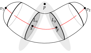
Figure 1: Bisector foliated by complex geodesics.

The bisector $B$ with real spine $G=\mathbb{P}_{\mathbb{C}}(W)$ also admits the meridional decomposition

$$B=\bigcup_{\varepsilon\in\mathbb{S}^{1}}\mathbb{P}_{\mathbb{C}}\big{(}W+\mathbb{R}\varepsilon p\big{)}\cap\mathbb{H}_{\mathbb{C}}^{2},$$

where $p\in V\setminus\{0\}$ is a fixed representative of the polar point $p$ of the complex spine $L$ and $\varepsilon\in\mathbb{S}^{1}$ is a unit complex number. Given $\varepsilon\in\mathbb{S}^{1}$, the $\mathbb{R}$-plane $\mathbb{P}_{\mathbb{C}}(W+\mathbb{R}\varepsilon p)\cap\mathbb{H}_{\mathbb{C}}^{2}$ is called a meridian of the bisector. Every meridian of $B$ contains the real spine $G$. Each point $p\in B\setminus G$ is contained in a unique meridian $M$ of $B$ and determines a meridional curve which is the curve in $M$ through $p$ equidistant from $G$ (in other words, a hypercycle in the Beltrami-Klein disc $M$). We also define a meridional curve when $p\in B$ is isotropic. In this case, the intersection $M\cap\partial\mathbb{H}_{\mathbb{C}}^{2}$ is a circle divided by the vertices of $G$ into two semicircles; we take the one containing $p$.

Figure 2: Meridional decomposition.

A pair of ultraparallel complex geodesics $L_{1},L_{2}$ determines a unique bisector $B(L_{1},L_{2})$ whose real spine is the unique geodesic $G$ that is simultaneously orthogonal to $L_{1}$ and $L_{2}$. Explicitly, this geodesic can be constructed as follows. The projective lines containing $L_{1},L_{2}$ intersect at a positive point $p\in{\mathrm{E}}(V)$. The complex geodesic $\mathbb{P}_{\mathbb{C}}(p^{\perp})$ intersects $L_{i}$ at $c_{i}$, $i=1,2$, and $G=G(c_{1},c_{2})$. The segment of bisector $B[L_{1},L_{2}]$ is defined by

$$B[L_{1},L_{2}]:=\bigsqcup_{x\in G[c_{1},c_{2}]}L_{x},$$

where $L_{x}$ stands for the slice of $B[L_{1},L_{2}]$ through $x$. The slice of $B[L_{1},L_{2}]$ through the middle point of $G[c_{1},c_{2}]$ is called the middle slice of $B[L_{1},L_{2}]$.

2.4.  Holomorphic isometries

The group of holomorphic isometries of $\mathbb{H}_{\mathbb{C}}^{2}$ is the projective unitary group $\mathrm{\mathrm{PU}}(2,1)$. The special unitary group $\mathrm{\mathrm{SU}}(2,1)$ is a triple cover of $\mathrm{\mathrm{PU}}(2,1)$ (lifts differ by a cube root of unity) and we refer to elements in $\mathrm{\mathrm{SU}}(2,1)$ also as isometries.

In our construction of discrete group we essentially use elliptic isometries. An isometry $I\in\mathrm{\mathrm{SU}}(2,1)$ is said to be elliptic when it has a negative fixed point $c\in\mathbb{H}_{\mathbb{C}}^{2}$. In this case, the projective line $\mathbb{P}_{\mathbb{C}}(c^{\perp})$ is $I$-stable. So, the isometry has a fixed point $p\in\mathbb{P}_{\mathbb{C}}(c^{\perp})$. The point $q\in\mathbb{P}_{\mathbb{C}}(c^{\perp})$ which is orthogonal to $p$ (see Remark 4) must also be fixed by $I$. In other words, there is an orthogonal basis in $V$ formed by eigenvectors of $I$. Let $\varepsilon_{1},\varepsilon_{2},\varepsilon_{3}\in\mathbb{C}$ with $\varepsilon_{1}\varepsilon_{2}\varepsilon_{3}=1$ be the eigenvalues corresponding respectively to $c,p,q$. Since none of $c,p,q$ is isotropic, we have $|\varepsilon_{i}|=1$ for $i=1,2,3$. It is straightforward to see that $I$ is given by the rule

$$I:x\mapsto(\varepsilon_{1}-\varepsilon_{3})\frac{\langle x,c\rangle}{\langle c,c\rangle}c+(\varepsilon_{2}-\varepsilon_{3})\frac{\langle x,p\rangle}{\langle p,p\rangle}p+\varepsilon_{3}x.$$ (5)

The isometry $I$ is called regular elliptic if its eigenvalues are pairwise distinct and special elliptic otherwise. We may describe the geometry of regular and special elliptic isometries as follows.

The regular elliptic case. The points $c,p,q$ are the only fixed points of $I$. We call $c$ the center of the isometry. The complex geodesics $\mathbb{P}_{\mathbb{C}}(p^{\perp})$ and $\mathbb{P}_{\mathbb{C}}(q^{\perp})$ intersect orthogonally at $c$ and both are $I$-stable. There are no other $I$-stable complex geodesics. Moreover, $I$ acts on $\mathbb{P}_{\mathbb{C}}(p^{\perp})\cap\mathbb{H}_{\mathbb{C}}^{2}$ as the rotation about $c$ by the angle $\mathrm{\mathrm{Arg}}(\varepsilon_{1}^{-1}\varepsilon_{3})$ and on $\mathbb{P}_{\mathbb{C}}(q^{\perp})\cap\mathbb{H}_{\mathbb{C}}^{2}$ as the rotation about $c$ by the angle $\mathrm{\mathrm{Arg}}(\varepsilon_{1}^{-1}\varepsilon_{2})$.

The special elliptic case. We can assume that not all eigenvalues of $I$ are equal (for otherwise, $I$ acts identically on $\mathbb{P}_{\mathbb{C}}(V)$). Hence, exactly one of the projective lines $\mathbb{P}_{\mathbb{C}}(c^{\perp})$, $\mathbb{P}_{\mathbb{C}}(p^{\perp})$, or $\mathbb{P}_{\mathbb{C}}(q^{\perp})$ is pointwise fixed by $I$. If the pointwise fixed line is $\mathbb{P}_{\mathbb{C}}(c^{\perp})$, that is, if $\varepsilon_{2}=\varepsilon_{3}$, then every complex geodesic that passes through $c$ is $I$-stable, the isometry acts on such complex geodesic as the rotation about $c$ by the angle $\mathrm{\mathrm{Arg}}(\varepsilon_{1}^{-1}\varepsilon_{2})$, and there are no other $I$-stable complex geodesics. In this case, we call $c$ the center of $I$ as well. When $\mathbb{P}_{\mathbb{C}}(p^{\perp})$ is pointwise fixed ($\varepsilon_{1}=\varepsilon_{3}$), every complex geodesic intersecting $\mathbb{P}_{\mathbb{C}}(p^{\perp})$ orthogonally in a negative point is stable under $I$, the isometry acts on such complex geodesics as the rotation about the intersection point by the angle $\mathrm{\mathrm{Arg}}(\varepsilon_{1}^{-1}\varepsilon_{2})$, and there are no other $I$-stable complex geodesics. In other words, $I$ is a rotation with the axis $\mathbb{P}_{\mathbb{C}}(p^{\perp})\cap\mathbb{H}_{\mathbb{C}}^{2}$. The same is true for a rotation with the axis $\mathbb{P}_{\mathbb{C}}(q^{\perp})\cap\mathbb{H}_{\mathbb{C}}^{2}$. An important particular case of rotation about an axis is the reflection in a complex geodesic $L=\mathbb{P}_{\mathbb{C}}(p^{\perp})\cap\mathbb{H}_{\mathbb{C}}^{2}$ given by the involution $x\mapsto-x+2\frac{\langle x,p\rangle}{\langle p,p\rangle}p$ (taking $\varepsilon_{1}=\varepsilon_{3}=-\varepsilon_{2}=-1$ in expression (5)).

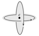
(a)

(b)

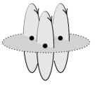
(c)

Figure 3: (a) Rotations about $c$ on two orthogonal complex geodesics by distinct angles, (b) Rotation about point, and (c) Rotation about complex line.

3 The turnover and its $\mathrm{\mathrm{PU}}(2,1)$-character variety

3.1.  The turnover

The group

$$G(n_{1},n_{2},n_{3}):=\langle g_{1},g_{2},g_{3}\mid g_{1}^{n_{1}}=g_{2}^{n_{2}}=g_{3}^{n_{3}}=1{\text{ \rm and }}g_{3}g_{2}g_{1}=1\rangle$$

is called the (hyperbolic) turnover, where $n_{1}$, $n_{2}$, $n_{3}$ are positive integers satisfying $\sum\limits_{j=1}^{3}\frac{1}{n_{j}}<1$.

We typically write simply $G$ in place of $G(n_{1},n_{2},n_{3})$. It is well-known that $G$ has a discrete cocompact action on the real hyperbolic plane $\mathbb{H}^{2}_{\mathbb{R}}$. Indeed, take a geodesic triangle $\Delta\subset\mathbb{H}^{2}_{\mathbb{R}}$ with interior angles $\pi/n_{1},\pi/n_{2},\pi/n_{3}$ and let $H(n_{1},n_{2},n_{3})$ denote the triangle group generated by the reflections $r_{1},r_{2},r_{3}$ in the sides of $\Delta$. The turnover $G$ appears as the index $2$ subgroup in $H$ generated by the rotations $g_{1}:=r_{1}r_{2}$, $g_{2}:=r_{3}r_{1}$, $g_{3}:=r_{2}r_{3}$. By the Poincaré Polyhedron Theorem, the quadrilateral $P:=\Delta\cup r_{2}\Delta$ with the vertices, sides, and side-pairings indicated in Picture 4, is a fundamental domain for the action of $G$ on $\mathbb{H}_{\mathbb{R}}^{2}$.

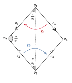
(a)

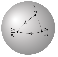
(b)

Figure 4: (a) Fundamental domain for $G$ and (b) Orbifold $\mathbb{S}^{2}(n_{1},n_{2},n_{3})$

The orbifold $\mathbb{H}_{\mathbb{R}}^{2}/G$ is the $2$-sphere $\mathbb{S}^{2}(n_{1},n_{2},n_{3})$ with $3$ cone points of angles $2\pi/n_{1},2\pi/n_{2},2\pi/n_{3}$ and orbifold Euler characteristic (see [Sco])

$$\chi=-1+\frac{1}{n_{1}}+\frac{1}{n_{2}}+\frac{1}{n_{3}}.$$

3.2.  Character variety

In this subsection, we deal with the space $\mathcal{R}$ of conjugacy classes of representations $\rho:G\to\mathrm{\mathrm{PU}}(2,1)$, where $G$ is the turnover group defined in Subsection 3.1. More precisely, the turnover group $G:=G(n_{1},n_{2},n_{3})$ acts on the space $\mathrm{Hom}\big{(}G,\mathrm{\mathrm{PU}}(2,1)\big{)}$ of all group homomorphisms from $G$ to $\mathrm{\mathrm{PU}}(2,1)$ by conjugation, i.e., $g\rho:h\mapsto\rho(g)\rho(h)\rho(g)^{-1}$. The $\mathrm{\mathrm{PU}}(2,1)$-character variety of $G$ is the quotient

$$\mathcal{R}(n_{1},n_{2},n_{3}):=\mathrm{Hom}\big{(}G,\mathrm{\mathrm{PU}}(2,1)\big{)}/G.$$

Usually, we denote $\mathcal{R}(n_{1},n_{2},n_{3})$ by $\mathcal{R}$.

Let $\rho:G\to\mathrm{\mathrm{PU}}(2,1)$ be a faithful $\mathrm{\mathrm{PU}}(2,1)$-representation of the turnover group. Then each isometry $I_{j}:=\rho(g_{j})$ is elliptic because a non-identical finite-order isometry in $\mathrm{\mathrm{PU}}(2,1)$ is necessarily elliptic. Let us see how the $\mathrm{\mathrm{PU}}(2,1)$-representations of the turnover depend on the nature of the elliptic isometries $I_{1}$, $I_{2}$, $I_{3}$.

A representation $\rho:G\to\mathrm{\mathrm{PU}}(2,1)$ is called $\mathbb{C}$-plane if it stabilizes a projective line in $\mathbb{P}_{\mathbb{C}}(V)$ or, equivalently, if it possesses a fixed point in $\mathbb{P}_{\mathbb{C}}(V)$. Some components of $\mathcal{R}$ are $\mathbb{C}$-plane:

Lemma 6.

If at least two of the $I_{j}$’s are special elliptic isometries, then $\rho$ is $\mathbb{C}$-plane.

Proof. A special elliptic isometry has a pointwise fixed projective line (see Section 2). Hence, we can find a point that is simultaneously fixed by two special elliptic isometries among $I_{j}$, $j=1,2,3$. This point must also be fixed by the remaining isometry due to the relation $I_{3}I_{2}I_{1}=1$. _■

A $\mathbb{C}$-plane representation is induced from a representation of the turnover in the isometry group of a stable complex geodesic. The well-known $\mathbb{C}$-Fuchsian representations (see [Kap2]) are constructed in this way and they lead to the complex hyperbolic $\mathbb{C}$-Fuchsian disc bundles. We will not deal with $\mathbb{C}$-plane representations here as we focus on the generic case.

We now consider the case where at least two of the $I_{j}^{\prime}$’s are regular elliptic. So, assume that $I_{1}$ and $I_{3}$ are regular elliptic.

We can choose representatives for the isometries $I_{1},I_{2},I_{3}$ in $\mathrm{\mathrm{SU}}(2,1)$ with respective eigenvalues $\alpha_{j},\beta_{j},\gamma_{j}^{-1}$, $j=1,2,3$, satisfying $I_{3}I_{2}I_{1}=1$. The eigenvalues denoted with index $1$ correspond to a negative eigenvector. Since $I_{1},I_{3}$ are regular elliptic, we have $\alpha_{i}\neq\alpha_{j}$ and $\gamma_{i}\neq\gamma_{j}$ for $i\neq j$. For $I_{2}$, there are three possibilities. It can be regular elliptic ($\beta_{i}\neq\beta_{j}$ for $i\neq j$), a rotation about a point in $\mathbb{H}_{\mathbb{C}}^{2}$ ($\beta_{2}=\beta_{3}$), or a rotation around a complex geodesic ($\beta_{1}=\beta_{2}$ or $\beta_{1}=\beta_{3}$).

So, in order to find all possible faithful representations of the turnover $G(n_{1},n_{2},n_{3})$ in $\mathrm{\mathrm{PU}}(2,1)$ we fix

$$(\alpha_{1},\alpha_{2},\alpha_{3}),(\beta_{1},\beta_{2},\beta_{3}),(\gamma_{1},\gamma_{2},\gamma_{3})\in\mathbb{S}^{1}\times\mathbb{S}^{1}\times\mathbb{S}^{1}$$

of order $3n_{1},3n_{2},3n_{3}$, respectively, satisfying

$$\alpha_{1}\alpha_{2}\alpha_{3}=\beta_{1}\beta_{2}\beta_{3}=\gamma_{1}\gamma_{2}\gamma_{3}=1,$$

$$\alpha_{i}\neq\alpha_{j},\quad\gamma_{i}\neq\gamma_{j}\quad for\quad i\neq j,$$

$$\alpha_{i}^{n_{1}}=\alpha_{j}^{n_{1}},\quad\beta_{i}^{n_{2}}=\beta_{j}^{n_{2}},\quad\gamma_{i}^{n_{3}}=\gamma_{j}^{n_{3}}\quad for\quad i\neq j,$$

and a regular elliptic isometry $I_{1}$ with eigenvalues $\alpha_{j}$. We look for all $I_{2}$ such that

$$\mathrm{\mathrm{tr}}(I_{2}I_{1})=\sum\limits_{j=1}^{3}\gamma_{j}.$$

It follows from [Gol1, p. 204, Theorem 6.2.4] that this trace equation holds iff $I_{3}:=(I_{2}I_{1})^{-1}$ is a regular elliptic isometry with eigenvalues $\gamma_{j}^{-1}$. This strategy allows us to prove the Proposition 8.

Definition 7.

Let $\rho$ be a faithful representation where none of the $\rho g_{j}$’s is special elliptic. We call the representation generic if there exists $i\neq j$ such that the fixed points of $\rho(g_{i})$ and $\rho(g_{j})$ are pairwise non-orthogonal (see also 17).

Proposition 8.

Let $\rho:G\to\mathrm{\mathrm{PU}}(2,1)$ be a faithful representation. If exactly one of the $\rho g_{j}$’s is special elliptic, then $\rho$ is rigid. Assume that none of the $\rho g_{j}$’s is special elliptic. If $\rho$ is generic, the corresponding component of $\mathcal{R}$ has dimension $2$; otherwise, the dimension is bounded by $1$.

Section 4 is devoted to the proof of the above proposition.

Every disc bundle constructed in [AGG] corresponds to a rigid representation $\rho:G\to\mathrm{\mathrm{PU}}(2,1)$ for $G=G(n,2,n)$. Most of the examples highlighted in Section 4 correspond to representations lying in the two-dimensional component of $\mathcal{R}$.

Remark 9.

Whenever we deal with elliptic isometries $I_{1},I_{2},I_{3}$ we will assume that either:

• $I_{1},I_{2},I_{3}\in\mathrm{\mathrm{PU}}(2,1)$ with $I_{j}^{n_{j}}=I_{3}I_{2}I_{1}=1$ and $\sum\limits_{j=1}^{3}\frac{1}{n_{j}}<1$;

• $I_{1},I_{2},I_{3}\in\mathrm{\mathrm{SU}}(2,1)$ with $I_{j}^{n_{j}}=\delta_{j}$ and $I_{3}I_{2}I_{1}=1$, where $\delta_{j}\in\mathbb{C}$ is a cubic root of unity and $\sum\limits_{j=1}^{3}\frac{1}{n_{j}}<1$.

Whether we take the isometries in $\mathrm{\mathrm{PU}}(2,1)$ or in $\mathrm{\mathrm{SU}}(2,1)$ will be explicitly indicated or should be clear from the context.

4 Computational results

Let us first consider the faithful representation $G(n_{1},n_{2},n_{3})\to\mathrm{\mathrm{PU}}(2,1)$ where the isometries $I_{1}$, $I_{2}$, $I_{3}$ are regular elliptic with eigenvalues $\alpha_{i}$’s, $\beta_{i}$’s, and $\gamma_{i}^{-1}$’s, respectively, following the Subsection 3.2. In our computational investigation, we set the following eigenvalues:

$$\alpha_{1}=\exp\left(\frac{2(n_{1}-k_{1})\pi i}{3n_{1}}\right),\quad \alpha_{2}=\exp\left(\frac{2(n_{1}-k_{1}-3)\pi i}{3n_{1}}\right),\quad \alpha_{3}=\exp\left(\frac{2(2k_{1}+n_{1}+3)\pi i}{3n_{1}}\right),$$

$$\beta_{1}=\exp\left(\frac{-2k_{2}\pi i}{3n_{2}}\right),\quad \beta_{2}=\exp\left(\frac{2(-k_{2}-3)\pi i}{3n_{2}}\right),\quad \beta_{3}=\exp\left(\frac{2(2k_{2}+3)\pi i)}{3n_{2}}\right),$$

$$\gamma_{1}^{-1}=\exp\left(\frac{2(2n_{3}d-k_{3})\pi i}{3n_{3}}\right),\quad \gamma_{2}^{-1}=\exp\left(\frac{2(2n_{3}d-k_{3}-3)\pi i}{3n_{3}}\right),\quad \gamma_{3}^{-1}=\exp\left(\frac{2(2n_{3}d+2k_{3}+3)\pi i)}{3n_{3}}\right),$$

where $n_{1},n_{2},n_{3},k_{1},k_{2},k_{3},d$ are integers. We choose these parameters so the condition (Q4) is satisfied. Due to the properties of the exponential, we can impose $0\leq k_{i}\leq n_{i}-1$ and $d=0,1,2$. Since we are interested here in cases when the three isometries are regular elliptic, meaning the eigenvalues are pairwise distinct, we exclude here the cases where $k_{i}=n_{i}-2$ and $k_{i}=n_{i}-1$.

We have found $3464$ lists $(n_{1},n_{2},n_{3},k_{1},k_{2},k_{3})$, with $3\leq n_{i}\leq 15$ and $0\leq k_{i}\leq n_{i}-3$ and $d=1$, corresponding to faithful discrete representations. More precisely, we have $3464$ representations $G(n_{1},n_{2},n_{3})\to\mathrm{\mathrm{PU}}(2,1)$ that lead to disc orbibundles over spheres with three conic points. These are examples of disc orbibundles $\mathbb{H}_{\mathbb{C}}^{2}/G\to\mathbb{H}_{\mathbb{R}}^{2}/G$ as discussed in Subsection 7.1. Additionally, they are topologically distinct because they have different relative Euler numbers $e/\chi$. Of these $3464$ examples, $853$ distinct triples $(n_{1},n_{2},n_{3})$ occur, thus our examples take place in $853$ different character varieties. Passing to finite index, each of these disc orbibundles over an orbifold gives rise to a disc bundle over a surface with the same relative Euler number $e/\chi$ and the same relative Toledo invariant $\tau/\chi$ (for details about these invariants see [Bot1]).

By Proposition 8, each of these orbibundles belongs to a $2$-dimensional family of pairwise non-isometric (nevertheless, diffeomorphic) bundles. Clearly, examples in the same family share the same discrete invariants. The corresponding relative Euler numbers vary in the region $\{-1\}\cup(-0.63,0.49)$ and all examples satisfy the relation $3\tau=2(e+\chi)$, which is a necessary condition for the existence of a holomorphic section (see [Bot1, Corollary 43]).

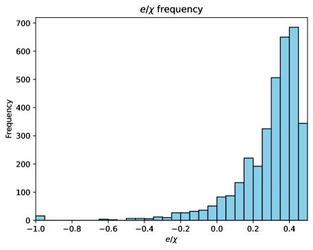
Figure 5: Histogram for the variable $e/\chi$. A total of $3464$ non-rigid disc orbibundles with different relative Euler numbers $e/\chi$ are found in $853$ character varieties.

A couple of examples deserve to be highlighted: the cotangent bundle ($e/\chi=-1$) and the trivial bundle ($e/\chi=0$). This seems to be the first instance of a complex hyperbolic structure on the cotangent bundle of a compact Riemann surface. As for the trivial bundle, an example has been constructed in [AGu] thus solving a long-standing conjecture [Eli, Open Question 8.1], [Gol2, p. 583], and [Sch, p. 14]. Our construction is quite different from the one in [AGu]; while the latter produces, at the orbibundle level, a single rigid example, the former leads to several two-dimensional families of such trivial orbibundles. Finally, we also find non-rigid discrete representations corresponding to disc orbibundles whose relative Toledo invariant vanishes and which are not $\mathbb{R}$-Fuchsian because, for such examples, $\mathrm{\mathrm{tr}}[I_{1},I_{2}]\not\in\mathbb{R}$ (it is well-known that $\mathbb{R}$-Fuchsian representations have vanishing Toledo invariant; in this regard, see also [CuG]). It is interesting to note that we have found $2$ examples with $e/\chi=-0.5$, thus corresponding to a square root of the cotangent bundle.

The connected components of the $\mathrm{\mathrm{PU}}(2,1)$-character variety $\mathcal{R}(n_{1},n_{2},n_{3})$ that we study are parametrized in the coordinates $(s,t)\in\mathbb{R}_{\geq 0}\times\mathbb{R}_{\geq 0}$, as described in Section 5. Once fixed the parameters $\alpha_{i}$’s, $\beta_{i}$’s, $\gamma_{i}^{-1}$’s we determine, when possible, $I_{1},I_{2},I_{3}$ via the following procedure: we start by fixing the isometry $I_{1}$ as a diagonal matrix with eigenvalues $\alpha_{1},\alpha_{2},\alpha_{3}$, then we compute the isometry $I_{2}$ entries as function of $(s,t)$, where its negative eigenvector is $u:=(\sqrt{1+s+t},\sqrt{s},\sqrt{t})$ and the rest of the information follows by imposing that $I_{2}$ has eigenvalues $\beta_{i}$’s and $I_{2}I_{1}$ has eigenvalues $\gamma_{i}$’s. By imposing that the eigenvalues for $I_{2}$ are $\beta_{1},\beta_{2},\beta_{3}$ we can write $I_{2}$ explicitly as function of its negative eigenvector $u$ associated to $\beta_{1}$ and a positive eigenvector $v$, associated to $\beta_{2}$, using the expression in Equation (14). This second eigenvector is determined by imposing that $I_{2}I_{1}$ have trace $\gamma_{1}+\gamma_{2}+\gamma_{3}$, which implies, by a result due to Goldman, that $I_{2}I_{1}$ has eigenvalues $\gamma_{1},\gamma_{2},\gamma_{3}$, assuming these three numbers are pairwise distinct. For details, see Regular case: $I_{2}$ is regular elliptic in the Section 5.

With that in mind, we list all examples found with $e/\chi=-1,\,-0.5,\,0$.

$n_{1}$	$n_{2}$	$n_{3}$	$k_{1}$	$k_{2}$	$k_{3}$	$s$	$t$	$e/\chi$
3	4	12	0	0	4	1.0	0.4	0
4	3	12	0	0	4	0.7	0.5	0
5	3	15	0	0	6	1.2	1.0	0
5	3	15	1	0	3	1.2	0.4	0
5	5	5	0	2	0	2.4	0.9	0
6	4	12	0	0	6	3.8	2.7	0
8	4	8	4	0	0	3.5	0.7	0
9	3	9	0	0	4	3.5	2.6	0
9	3	9	1	0	3	2.9	1.0	0
9	3	9	3	0	1	2.6	0.4	0
9	3	9	4	0	0	2.4	0.2	0
12	3	4	4	0	0	2.9	0.3	0
12	3	12	6	0	0	3.4	0.3	0
12	4	3	4	0	0	3.7	0.6	0
15	3	5	6	0	0	4.4	0.3	0
3	3	9	0	0	1	0.6	0.4	-0.5
9	3	3	1	0	0	2.5	1.2	-0.5

$n_{1}$	$n_{2}$	$n_{3}$	$k_{1}$	$k_{2}$	$k_{3}$	$s$	$t$	$e/\chi$
3	3	4	0	0	0	0.3	0.2	-1
3	3	5	0	0	0	0.5	0.3	-1
3	3	6	0	0	0	0.6	0.4	-1
3	3	7	0	0	0	0.7	0.5	-1
3	4	3	0	0	0	0.4	0.4	-1
4	3	3	0	0	0	0.3	0.4	-1
4	3	4	0	0	0	0.7	0.7	-1
4	3	5	0	0	0	1.1	1.1	-1
4	3	6	0	0	0	1.4	1.4	-1
5	3	3	0	0	0	0.7	0.9	-1
5	3	4	0	0	0	1.5	1.6	-1
5	3	5	0	0	0	2.3	2.3	-1
6	3	3	0	0	0	1.4	1.6	-1
6	3	4	0	0	0	2.8	2.8	-1
7	3	3	0	0	0	2.2	2.4	-1
8	3	3	0	0	0	3.4	3.6	-1

Table 1: Non-rigid examples with $e/\chi$ equal to $0,-0.5,-1$.

The methodology followed to find examples is the following: for each $(n_{1},n_{2},n_{3},k_{1},k_{2},k_{3},d)$, with $3\leq n_{i}\leq 15$, $0\leq k_{i}\leq n_{i}-3$ and $d=1$, we constructed the representation following the formulas in Section 5 and then tested the conditions for discreteness, described in Section 6 and more in-depth in Subsection 7.1 for $s,t\in(0.1\mathbb{Z})\cap[0,5]$. We found $39431$ examples. Among them, we observed $853$ distinct $(n_{1},n_{2},n_{3},k_{1},k_{2},k_{3},d)$ with different Euler numbers $e/\chi$ (the relative Euler number does not depend on the parameters $s,t$), thus corresponding to distinct topological objects.

Remark 10.

Explicit computations can be found in the Section 9 for the example

$$(n_{1},n_{2},n_{3},k_{1},k_{2},k_{3},s,t)=(5,5,5,0,2,0,2.4,0.9),$$

from the Table 1 above. Such representation is discrete forming a disc orbibundle over $\mathbb{S}^{2}(5,5,5)$. Additionally, we compute its Euler number to be $e=0$ and the Toledo invariant to be $\tau=\frac{3}{2}\chi$.

We illustrate below a prototypical connected component of $\mathcal{R}(3,3,4)$ in the coordinates $(s,t)$. The precise parameters for this component are $n_{1}=n_{2}=3,n_{3}=4,k_{1}=k_{2}=k_{3}=0$, as shown in Table 1.

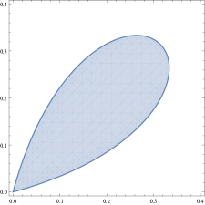
Figure 6: $\mathcal{R}(3,3,4)$ with regular $I_{1},I_{2},I_{3}$

In all the cases we considered, $\mathcal{R}(n_{1},n_{2},n_{3})$ is a disjoint union of topological discs. The shaded region in Figure 7 corresponds to a family of disc orbibundles (see Subsection 7.1), i.e, a pair of distinct points in the shaded region corresponds to a pair of diffeomorphic but non-isometric disc orbibundles.

Figure 7: Some disc orbibundles over $\mathbb{S}^{2}(3,3,4)$

In principle, it could be that all faithful representations $G(n_{1},n_{2},n_{3})\to\mathrm{\mathrm{PU}}(2,1)$ with regular $I_{1},I_{2},I_{3}$ were discrete; for a point in the above shaded region, discreteness is guaranteed because a particular fundamental domain is shown to exist (see Section 6), but nothing is preventing the points outside such region to also correspond to discrete representations. However, this is not the case. Indeed, consider the function $G(s,t)=f(\mathrm{\mathrm{tr}}[I_{1},I_{2}])$, where

$$f(z)=|z|^{4}-8(z^{3})+18|z|^{2}-27$$

is Goldman’s discriminant (see [Gol1, p. 204, Theorem 6.2.4]). The region in $\mathcal{R}(3,3,4)$ described by $G(s,t)<0$ is the shaded area in the Figure 8. Note that $G(0.01,0.01)\simeq-12.282$ is negative and $G(0.05,0.05)=26.392$ is positive.

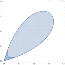
Figure 8: $\mathcal{R}(3,3,4)$ and $\mathrm{\mathrm{G}}(s,t)<0$

Not all examples with $G(s,t)<0$ can be discrete because, by [Gol1, Theorem 6.2.4], $G(s,t)<0$ means that $[I_{1},I_{2}]$ is regular elliptic. Since in $\mathcal{R}(3,3,4)$ there are also points where $G(s,t)>0$, we obtain uncountable many distinct negative values for $G(s,t)$. If all representations in $\mathcal{R}(3,3,4)$ were discrete, the elliptic isometries in the group $\langle I_{1},I_{2},I_{3}\rangle$ would be of finite order, since discrete groups of isometries have finite stabilizers, leading to a countable amount of possibles values for $G(s,t)<0$. By continuity, there is a non-discrete faithful representation with $s=t$ and $t\in(0.01,0.05)$.

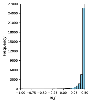
(a)

(b)

Figure 9: (a) Histogram for the variable $e/\chi$ when $I_{2}$ is a rotation about a point. A total of $34240$ rigid disc orbibundles with different relative Euler numbers $e/\chi$ are found in $13345$ character varieties. (b) Histogram for the variable $e/\chi$ when $I_{2}$ is a rotation about a complex geodesic. A total of $67769$ rigid disc orbibundles with different relative Euler numbers $e/\chi$ are found in $17030$ character varieties.

Now we discuss the representations where $I_{1},I_{3}$ are regular elliptic and $I_{2}$ is special elliptic with $3\leq n_{1},n_{3}\leq 30$, $0\leq k_{1}\leq n_{1}-3$, $0\leq k_{3}\leq n_{3}-3$, $2\leq n_{2}\leq 30$, $0\leq k_{2}\leq n_{2}-1$ and $d=0,1,2$. When $I_{2}$ is a rotation about a point ($\beta_{2}=\beta_{3}$), we found $34240$ examples in $13345$ different character varieties, with $e/\chi\in[-1,0.5]$. The values $e/\chi=-1,\,-0.5,\,0,\,0.5$ occur here. On the other hand, when $I_{2}$ is a rotation around a complex geodesic ($\beta_{1}=\beta_{3}$), we found $67769$ examples in $17030$ different character varieties, with $e/\chi\in(0,0.5]$, including the right extreme (thus neither $e/\chi=-1$ nor $e/\chi=0$ were observed here, the case $e/\chi=0.5$ occurs $50$ times, corresponding to square roots of tangent bundles). As in all the examples we found, the identity $3\tau=2(e+\chi)$ is satisfied. Note that $e/\chi=0.5$ is the maximal relative Euler number allowed by this formula (because $|\tau/\chi|\leq 1$ by Toledo Rigidity) and that this particular relative Euler number only happens for $\tau/\chi=1$ (thus, the corresponding representation is $\mathbb{C}$-Fuchsian).

We list all the rigid examples with $e/\chi=-1,\,-0.5,\,0,\,0.5$ on the Tables 2 and 3. On these table, there is no parameter $s,t$ displayed because they are determined by the eigenvalues when $I_{2}$ is a rotation about a point ($\beta_{2}=\beta_{3}$) and $I_{2}$ does not depend them when $I_{2}$ is a rotation about a geodesic ($\beta_{1}=\beta_{3}$), as can be seen from the formula for the matrix $I_{2}$ at the Equation (14).

$n_{1}$	$n_{2}$	$n_{3}$	$k_{1}$	$k_{2}$	$k_{3}$	$e/\chi$
16	16	8	0	14	2	0.5
18	6	5	0	4	1	0.5
18	12	12	0	10	4	0.5
18	15	30	0	13	12	0.5
19	19	19	0	17	7	0.5
19	19	19	16	17	10	0.5
20	15	12	0	13	4	0.5
20	20	30	0	18	12	0.5
23	23	23	0	21	9	0.5
24	4	24	0	2	12	0.5
24	8	3	0	6	0	0.5
24	8	5	0	6	1	0.5
24	8	7	0	6	2	0.5
24	8	9	0	6	3	0.5
24	8	11	0	6	4	0.5
24	8	13	0	6	5	0.5
24	8	15	0	6	6	0.5
24	8	17	0	6	7	0.5
24	8	19	0	6	8	0.5
24	8	21	0	6	9	0.5
24	8	23	0	6	10	0.5
24	8	25	0	6	11	0.5
24	8	27	0	6	12	0.5
24	8	29	0	6	13	0.5
24	12	24	0	10	10	0.5
24	24	12	0	22	4	0.5
25	5	5	1	3	1	0.5

$n_{1}$	$n_{2}$	$n_{3}$	$k_{1}$	$k_{2}$	$k_{3}$	$e/\chi$
25	25	25	20	23	15	0.5
25	5	25	22	3	15	0.5
25	25	25	22	23	13	0.5
27	3	27	0	1	15	0.5
27	9	3	0	7	0	0.5
27	9	5	0	7	1	0.5
27	9	7	0	7	2	0.5
27	9	9	0	7	3	0.5
27	9	11	0	7	4	0.5
27	9	13	0	7	5	0.5
27	9	15	0	7	6	0.5
27	9	17	0	7	7	0.5
27	9	19	0	7	8	0.5
27	9	21	0	7	9	0.5
27	9	23	0	7	10	0.5
27	9	25	0	7	11	0.5
27	9	27	0	7	12	0.5
27	9	29	0	7	13	0.5
27	3	27	24	1	18	0.5
27	6	18	24	4	10	0.5
27	9	9	24	7	4	0.5
27	9	27	24	7	15	0.5
27	18	30	24	16	16	0.5
30	4	20	0	2	10	0.5
30	10	3	0	8	0	0.5
30	10	5	0	8	1	0.5
30	10	7	0	8	2	0.5

$n_{1}$	$n_{2}$	$n_{3}$	$k_{1}$	$k_{2}$	$k_{3}$	$e/\chi$
30	10	9	0	8	3	0.5
30	10	13	0	8	5	0.5
30	10	15	0	8	6	0.5
30	10	17	0	8	7	0.5
30	10	19	0	8	8	0.5
30	10	21	0	8	9	0.5
30	10	23	0	8	10	0.5
30	10	27	0	8	12	0.5
30	10	29	0	8	13	0.5
5	2	10	0	0	2	0
5	2	10	1	0	0	0
7	2	14	1	0	2	0
7	2	14	2	0	0	0
8	2	8	0	0	2	0
8	2	8	2	0	0	0
10	2	5	0	0	1	0
10	2	5	2	0	0	0
12	2	12	4	0	0	0
14	2	7	2	0	1	0
14	2	7	4	0	0	0
18	2	9	4	0	1	0
18	2	9	6	0	0	0
22	2	11	8	0	0	0
9	2	6	1	0	0	-0.5
3	2	7	0	0	0	-1
3	2	8	0	0	0	-1
3	2	9	0	0	0	-1

$n_{1}$	$n_{2}$	$n_{3}$	$k_{1}$	$k_{2}$	$k_{3}$	$e/\chi$
3	2	10	0	0	0	-1
3	2	11	0	0	0	-1
3	2	12	0	0	0	-1
3	2	13	0	0	0	-1
3	2	14	0	0	0	-1
3	2	15	0	0	0	-1
3	2	16	0	0	0	-1
4	2	5	0	0	0	-1
4	2	6	0	0	0	-1
4	2	7	0	0	0	-1
4	2	8	0	0	0	-1
4	2	9	0	0	0	-1
5	2	4	0	0	0	-1
5	2	5	0	0	0	-1
5	2	6	0	0	0	-1
5	2	7	0	0	0	-1
6	2	4	0	0	0	-1
6	2	5	0	0	0	-1
7	2	3	0	0	0	-1
7	2	4	0	0	0	-1
7	2	5	0	0	0	-1
8	2	3	0	0	0	-1
8	2	4	0	0	0	-1
9	2	3	0	0	0	-1

Table 2: Rigid examples with $e/\chi$ equal to $0.5,0,-0.5,-1$ when $I_{2}$ is a rotation about a point. There are 27 instances with $e/\chi=-1$ , $1$ with $e/\chi=-0.5$, $14$ with $e/x=0$, and $63$ with $e/\chi=0.5$.

$n_{1}$	$n_{2}$	$n_{3}$	$k_{1}$	$k_{2}$	$k_{3}$	$e/\chi$
9	27	27	0	26	7	0.5
9	27	27	6	26	16	0.5
9	30	30	6	29	18	0.5
11	22	22	8	21	12	0.5
12	28	7	0	27	1	0.5
14	14	7	0	13	1	0.5
15	30	30	0	29	10	0.5
15	25	25	12	24	13	0.5
15	30	30	12	29	16	0.5
18	12	4	0	11	0	0.5
18	18	27	0	17	9	0.5
20	10	4	0	9	0	0.5
20	12	30	0	11	10	0.5

$n_{1}$	$n_{2}$	$n_{3}$	$k_{1}$	$k_{2}$	$k_{3}$	$e/\chi$
21	30	30	16	29	18	0.5
21	21	21	18	20	10	0.5
21	28	28	18	27	14	0.5
22	22	11	0	21	3	0.5
24	8	4	0	7	0	0.5
24	8	20	0	7	6	0.5
24	24	18	0	23	6	0.5
25	25	25	1	24	8	0.5
25	30	30	1	29	10	0.5
25	25	25	18	24	16	0.5
25	25	25	21	24	13	0.5
25	30	30	21	29	16	0.5
25	25	25	22	24	12	0.5

$n_{1}$	$n_{2}$	$n_{3}$	$k_{1}$	$k_{2}$	$k_{3}$	$e/\chi$
26	26	13	22	25	6	0.5
27	18	18	0	17	6	0.5
27	27	27	0	26	10	0.5
27	27	27	1	26	9	0.5
27	27	9	4	26	1	0.5
27	27	27	18	26	19	0.5
27	27	27	19	26	18	0.5
27	27	27	21	26	16	0.5
27	27	9	22	26	4	0.5
27	27	27	22	26	15	0.5
27	9	27	24	8	12	0.5
27	27	27	24	26	13	0.5
28	2	28	0	1	4	0.5

$n_{1}$	$n_{2}$	$n_{3}$	$k_{1}$	$k_{2}$	$k_{3}$	$e/\chi$
28	12	21	0	11	7	0.5
28	14	28	0	13	10	0.5
29	29	29	1	28	10	0.5
29	29	29	21	28	19	0.5
29	29	29	22	28	18	0.5
29	29	29	23	28	17	0.5
29	29	29	24	28	16	0.5
29	29	29	26	28	14	0.5
30	15	18	0	14	6	0.5
30	30	5	22	29	2	0.5
30	30	25	22	29	16	0.5

Table 3: We have found $50$ rigid examples with $e/\chi=0.5$ when $I_{2}$ is a rotation about a complex geodesic. No example with $e/\chi<0.16$ was found where $I_{2}$ is a rotation about a complex geodesic.

When we drop the transversalities conditions $\mathrm{Q2}$ and $\mathrm{Q3}$ stated in the subsection 6.2 for the quadrangles, the formula defining $e$ still makes sense, since it only depends on information coming from the eigenvalues of $I_{1},I_{2},I_{3}$ and on the integer $f$ defined in Subsection 7.6. Curiously, the formula $3\tau=2(e+\chi)$ still holds in the majority of the cases where the transversalities conditions were dropped. In the few cases where it fails, $3/2\tau-\chi$ differs from $e$ by an integer. This suggests that the formula for $f$ needs a correction with respect to the topology of the “quadrangle” corresponding to such degenerate cases. We believe that this corrected Euler number $e_{\text{cor}}:=3/2\tau-\chi$ have a geometrical meaning that is related to the object obtained by gluing the sides of the “quadrangle” respectively to the relations defined by $I_{1},I_{2},I_{3}$. Thus, in some sense, for all points in the character variety, it seems that there exists a geometric object that behaves as a bundle over $\mathbb{S}^{2}(n_{1},n_{2},n_{3})$ with Euler number $e_{\text{cor}}$.

5 Proof of proposition 8

In this section, we deal with the problem of finding elliptic isometries $I_{1},I_{2},I_{3}$ in $\mathrm{\mathrm{SU}}(2,1)$ that belong to prescribed conjugacy classes and satisfy $I_{3}I_{2}I_{1}=1$. The results lead to the parameterization of the representation space of the turnover group discussed in Section 3. We generalize the methods used in [AGG, Section 3].

Let $I_{1},I_{2},I_{3}\in\mathrm{\mathrm{SU}}(2,1)$ denote elliptic isometries in given conjugacy classes: $\alpha_{i}$, $\beta_{i}$, and $\gamma_{i}^{-1}$, $i=1,2,3$, stand respectively for the eigenvalues of $I_{1}$, $I_{2}$, and $I_{3}$. We will assume that the first eigenvalue of each $I_{i}$ corresponds to a negative eigenvector.

In view of Lemma 6 we assume that $I_{1},I_{3}$ are regular. In order to determine the $I_{i}$’s such that $I_{3}I_{2}I_{1}=1$ we fix the isometry $I_{1}$ and look for those $I_{2}$’s in $\mathrm{\mathrm{SU}}(2,1)$ satisfying the trace equation

$$\mathrm{\mathrm{tr}}(I_{2}I_{1})=\sum\limits_{i=1}^{3}\gamma_{i}.$$ (11)

By [Gol1, p. 204, Theorem 6.2.4], the trace equation holds if and only if $I_{2}I_{1}$ is a regular elliptic isometry with eigenvalues $\gamma_{1},\gamma_{2},\gamma_{3}$.

We consider separately the case where $I_{2}$ is regular elliptic and the case where $I_{2}$ special elliptic (the latter is broken into the rotation about a point in $\mathbb{H}_{\mathbb{C}}^{2}$ and rotation about a complex geodesic in $\mathbb{H}_{\mathbb{C}}^{2}$ subcases).

Regular case: $I_{2}$ is regular elliptic. Let $u,v\in V$ denote eigenvectors of $I_{2}$ corresponding to the eigenvalues $\beta_{1}$ and $\beta_{2}$. In particular, $u$ is negative and $v$ is positive. We fix a basis $\mathcal{B}$ in $V$ of signature $-++$ consisting of eigenvectors of $I_{1}$. The corresponding eigenvalues are $\alpha_{1},\alpha_{2},\alpha_{3}$. In this basis, we write

$$u=\left[\begin{smallmatrix}u_{1}\\ u_{2}\\ u_{3}\end{smallmatrix}\right],\quad v=\left[\begin{smallmatrix}v_{1}\\ v_{2}\\ v_{3}\end{smallmatrix}\right].$$

We can assume that

$$u_{1}>0,\quad u_{2},u_{3}\geq 0,\quad\langle u,u\rangle=-1,\quad v_{1},|v_{2}|,|v_{3}|\geq 0,\quad\langle v,v\rangle=1.$$

In other words,

$$-u_{1}^{2}+u_{2}^{2}+u_{3}^{2}=-1,\quad-v_{1}^{2}+|v_{2}|^{2}+|v_{3}|^{2}=1,\quad-u_{1}v_{1}+u_{2}v_{2}+u_{3}v_{3}=0.$$ (12)

(The last equality means that $\langle u,v\rangle=0$.)

In what follows, we show that $u_{2},u_{3}$ provide parameters that describe the component of the character variety $\mathcal{R}$ (see Subsection 3.2 for the definition) corresponding to the given conjugacy classes of $I_{1},I_{2},I_{3}$. Roughly speaking, the isometry $I_{2}$ is essentially determined, under certain conditions, by $u_{2},u_{3}>0$ and the trace equation. Note that the basis $\mathcal{B}$ defines the $\mathbb{R}$-plane $\mathbb{P}(W)\subset\mathbb{H}_{\mathbb{C}}^{2}$, where $W\subset V$ is spanned over $\mathbb{R}$ by $\mathcal{B}$. This $\mathbb{R}$-plane is exactly the one containing the fixed points of $I_{1}$ and the center $u$ of $I_{2}$. Varying $u_{2},u_{3}>0$ is the same as moving $u$ inside $\mathbb{P}(W)\cap\mathbb{B}$.

First, let us write down the trace equation (11) in the basis $\mathcal{B}$. We define

$$\sqrt{s}:=u_{2},\quad\sqrt{t}:=u_{3},\quad\beta_{ij}:=\beta_{i}-\beta_{j},\quad\alpha_{ij}:=\alpha_{i}-\alpha_{j},$$ (13)

for $i,j=1,2,3$. Hence, $u_{1}=\sqrt{1+s+t}$ and $\alpha_{ij},\beta_{ij}\neq 0$ if $i\neq j$. Using (5), we can write $I_{1},I_{2}$ in the basis $\mathcal{B}$ :

$$I_{1}=\left[\begin{smallmatrix}\alpha_{1}&0&0\\ 0&\alpha_{2}&0\\ 0&0&\alpha_{3}\end{smallmatrix}\right],\qquad I_{2}=\left[\begin{smallmatrix}-v_{1}^{2}\beta_{23}+u_{1}^{2}\beta_{13}+\beta_{3}&v_{1}\overline{v}_{2}\beta_{23}-u_{2}u_{1}\beta_{13}&v_{1}\overline{v}_{3}\beta_{23}-u_{3}u_{1}\beta_{13}\\ -v_{1}v_{2}\beta_{23}+u_{1}u_{2}\beta_{13}&|v_{2}|^{2}\beta_{23}-u_{2}^{2}\beta_{13}+\beta_{3}&v_{2}\overline{v}_{3}\beta_{23}-u_{3}u_{2}\beta_{13}\\ -v_{1}v_{3}\beta_{23}+u_{1}u_{3}\beta_{13}&\overline{v}_{2}v_{3}\beta_{23}-u_{2}u_{3}\beta_{13}&|v_{3}|^{2}\beta_{23}-u_{3}^{2}\beta_{13}+\beta_{3}\end{smallmatrix}\right].$$ (14)

The trace equation (11) takes the form

$$\alpha_{1}(-v_{1}^{2}\beta_{23}+u_{1}^{2}\beta_{13}+\beta_{3})+\alpha_{2}\big{(}|v_{2}|^{2}\beta_{23}-u_{2}^{2}\beta_{13}+\beta_{3}\big{)}+\alpha_{3}\big{(}|v_{3}|^{2}\beta_{23}-u_{3}^{2}\beta_{13}+\beta_{3}\big{)}=\sum_{i=1}^{3}\gamma_{i}$$

which is equivalent to

$$|v_{2}|^{2}\alpha_{21}+|v_{3}|^{2}\alpha_{31}=\frac{\beta_{13}}{\beta_{23}}\big{(}\alpha_{21}s+\alpha_{31}t\big{)}+k$$ (15)

in view of the first two equalities in (12) and in (13), where

$$k:=\frac{1}{\beta_{23}}\left(\sum\limits_{i=1}^{3}\gamma_{i}-\alpha_{1}(\beta_{1}+\beta_{2}-\beta_{3})-\beta_{3}(\alpha_{2}+\alpha_{3})\right).$$

We rewrite equation (15) so that $|v_{2}|^{2}$ and $|v_{3}|^{2}$ are explicitly given in terms of $s$ and $t$ :

Lemma 16.

The determinant of $M:=\left[\begin{smallmatrix}\alpha_{21}&\alpha_{31}\\ \mathrm{\mathrm{Im}}\alpha_{21}&\mathrm{\mathrm{Im}}\alpha_{31}\end{smallmatrix}\right]$ does not vanish. The trace equation is equivalent to the equations

$$|v_{2}|^{2}\det M=s\mathrm{\mathrm{Im}}\frac{\alpha_{31}\overline{\alpha}_{21}\overline{\beta}_{13}}{\overline{\beta}_{23}}+t|\alpha_{31}|^{2}\mathrm{\mathrm{Im}}\frac{\overline{\beta}_{13}}{\overline{\beta}_{23}}+\mathrm{\mathrm{Im}}(\alpha_{31}\overline{k}),$$

$$|v_{3}|^{2}\det M=s|\alpha_{21}|^{2}\mathrm{\mathrm{Im}}\frac{\beta_{13}}{\beta_{23}}+t\mathrm{\mathrm{Im}}\frac{\overline{\alpha}_{21}\alpha_{31}\beta_{13}}{\beta_{23}}+\mathrm{\mathrm{Im}}(\overline{\alpha}_{21}k).$$

The coefficient of $t$ in the first equation and that of $s$ in the second equation do not vanish.

Proof. Note that $|\det M|$ is twice the area of the triangle with vertices $\alpha_{1},\alpha_{2},\alpha_{3}$ in the unit circle. Since $\alpha_{1},\alpha_{2},\alpha_{3}$ are pairwise distinct, this triangle has non-vanishing area. Similarly, $\mathrm{\mathrm{Im}}\displaystyle\frac{\beta_{13}}{\beta_{23}}\neq 0$ because $\displaystyle\frac{\beta_{13}}{\beta_{23}}$ determines an internal angle of the triangle with vertices $\beta_{1},\beta_{2},\beta_{3}$.

The trace equation (11) is equivalent to

$$|v_{2}|^{2}\alpha_{21}+|v_{3}|^{2}\alpha_{31}=z,\qquad|v_{2}|^{2}\mathrm{\mathrm{Im}}\alpha_{21}+|v_{3}|^{2}\mathrm{\mathrm{Im}}\alpha_{31}=\mathrm{\mathrm{Im}}z,$$

where $z:=\displaystyle\frac{\beta_{13}}{\beta_{23}}\big{(}\alpha_{21}s+\alpha_{31}t\big{)}+k$. Hence,

$$|v_{2}|^{2}\det M=\mathrm{\mathrm{Im}}\alpha_{31}z-\alpha_{31}\mathrm{\mathrm{Im}}z=\mathrm{\mathrm{Im}}(\alpha_{31}\overline{z}),$$

$$|v_{3}|^{2}\det M=\alpha_{21}\mathrm{\mathrm{Im}}z-\mathrm{\mathrm{Im}}\alpha_{21}z=-\mathrm{\mathrm{Im}}(\alpha_{21}\overline{z}).$$ _■

Remark 17.

Let us deal with the case where the representation of the turnover providing the isometries $I_{1},I_{2},I_{3}$ is not generic (see Definition 7). If $s=0$ or $t=0$, rechoosing the basis $\mathcal{B}$ and using the third equation in (12), we can assume that $v_{2},v_{3}\geq 0$. Now, the values of $v_{2},v_{3}$ are determined by Lemma 16. So, we assume $s,t>0$. If $v_{1}=0$, then $u_{2}v_{3}=-u_{3}v_{3}$ by the third equation in (12) and $|v_{2}|,|v_{3}|$ are determined by Lemma 16. This implies that the representation space (modulo conjugation) constrained by $v_{1}=0$ have dimension at most $1$.

In view of the previous remark, from now on, we assume that the representation of the turnover providing the isometries $I_{1},I_{2},I_{3}$ is generic.

By Lemma 16, the trace equation and the second equation in (12) imply the following inequalities:

$$\begin{matrix}\displaystyle\frac{1}{\det M}\big{(}s\mathrm{\mathrm{Im}}\displaystyle\frac{\alpha_{31}\overline{\alpha}_{21}\overline{\beta}_{13}}{\overline{\beta}_{23}}+t|\alpha_{31}|^{2}\mathrm{\mathrm{Im}}\frac{\overline{\beta}_{13}}{\overline{\beta}_{23}}+\mathrm{\mathrm{Im}}(\alpha_{31}\overline{k})\big{)}>0,\par\\ \\ \displaystyle\frac{1}{\det M}\big{(}s|\alpha_{21}|^{2}\mathrm{\mathrm{Im}}\displaystyle\frac{\beta_{13}}{\beta_{23}}+t\mathrm{\mathrm{Im}}\frac{\overline{\alpha}_{21}\alpha_{31}\beta_{13}}{\beta_{23}}+\mathrm{\mathrm{Im}}(\overline{\alpha}_{21}k)\big{)}>0,\par\\ \\ \displaystyle\frac{1}{\det M}\Big{(}s\big{(}|\alpha_{21}|^{2}\mathrm{\mathrm{Im}}\frac{\beta_{13}}{\beta_{23}}+\mathrm{\mathrm{Im}}\frac{\alpha_{31}\overline{\alpha}_{21}\overline{\beta}_{13}}{\overline{\beta}_{23}}\big{)}\par\\ \\ \displaystyle\hskip 71.13188pt+t\big{(}|\alpha_{31}|^{2}\mathrm{\mathrm{Im}}\frac{\overline{\beta}_{13}}{\overline{\beta}_{23}}+\mathrm{\mathrm{Im}}\frac{\overline{\alpha}_{21}\alpha_{31}\beta_{13}}{\beta_{23}}\big{)}+\mathrm{\mathrm{Im}}(\alpha_{31}\overline{k}+\overline{\alpha}_{21}k)\Big{)}-1>0.\end{matrix}$$ (C1)

Conversely, if Condition C1 holds for a pair $(s,t)\in\mathbb{R}_{>0}\times\mathbb{R}_{>0}$ of positive real numbers, then the equations in Lemma 16 and the second equation in (12) provide the positive real numbers $v_{1},|v_{2}|,|v_{3}|$.

In the lemma below, we state a condition, referred to as Condition C2, that characterizes the possibility of expressing $v_{2}$ and $v_{3}$ in terms of $s,t,v_{1},|v_{2}|,|v_{3}|$.

Lemma 18.

We have

$$v_{2}=\frac{1}{2v_{1}\sqrt{s(1+s+t)}}\big{(}-t|v_{3}|^{2}+(1+s+t)v_{1}^{2}+s|v_{2}|^{2}\pm i\sqrt{\Delta}\big{)},$$

$$v_{3}=\frac{1}{2v_{1}\sqrt{t(1+s+t)}}\big{(}-s|v_{2}|^{2}+(1+s+t)v_{1}^{2}+t|v_{3}|^{2}\mp i\sqrt{\Delta}\big{)},$$

where

$$\Delta:=4v_{1}^{2}|v_{2}|^{2}s(1+s+t)-\big{(}-t|v_{3}|^{2}+(1+s+t)v_{1}^{2}+s|v_{2}|^{2}\big{)}^{2}\geq 0.$$ (C2)

Reciprocally, let $s,t,v_{1},|v_{2}|,|v_{3}|$ be given positive real numbers such that $-v_{1}^{2}+|v_{2}|^{2}+|v_{3}|^{2}=1$ and $\Delta\geq 0$. Then $v_{2},v_{3}$ are well defined in terms of $s,t,v_{1},|v_{2}|,|v_{3}|$ as above and satisfy $-u_{1}v_{1}+u_{2}v_{2}+u_{3}v_{3}=0$.

Proof. The third equality in 12 implies that $\,v_{3}=\displaystyle\frac{u_{1}v_{1}-u_{2}\,v_{2}}{u_{3}}$ and $\mathrm{\mathrm{Im}}\,v_{3}=-\displaystyle\frac{u_{2}\mathrm{\mathrm{Im}}\,v_{2}}{u_{3}}$. So,

$$|v_{3}|^{2}=\displaystyle\frac{(u_{1}v_{1}-u_{2}\,v_{2})^{2}+u_{2}^{2}(\mathrm{\mathrm{Im}}\,v_{2})^{2}}{u_{3}^{2}}=\frac{u_{1}^{2}v_{1}^{2}-2v_{1}u_{1}u_{2}\,v_{2}+u_{2}^{2}|v_{2}|^{2}}{u_{3}^{2}},$$

that is, $\,v_{2}=\displaystyle\frac{-u_{3}^{2}|v_{3}|^{2}+u_{1}^{2}v_{1}^{2}+u_{2}^{2}|v_{2}|^{2}}{2v_{1}u_{1}u_{2}}.$ It follows that

$$\mathrm{\mathrm{Im}}\,v_{2}=\frac{\sigma_{1}}{2v_{1}u_{1}u_{2}}\sqrt{4v_{1}^{2}|v_{2}|^{2}u_{1}^{2}u_{2}^{2}-\big{(}-u_{3}^{2}|v_{3}|^{2}+u_{1}^{2}v_{1}^{2}+u_{2}^{2}|v_{2}|^{2}\big{)}^{2}},$$

where $\sigma_{1}\in\{-1,1\}$. By symmetry, $\,v_{3}=\displaystyle\frac{-u_{2}^{2}|v_{2}|^{2}+u_{1}^{2}v_{1}^{2}+u_{3}^{2}|v_{3}|^{2}}{2v_{1}u_{1}u_{3}}$ and

$$\mathrm{\mathrm{Im}}\,v_{3}=\frac{\sigma_{2}}{2v_{1}u_{1}u_{3}}\sqrt{4v_{1}^{2}|v_{3}|^{2}u_{1}^{2}u_{3}^{2}-\big{(}-u_{2}^{2}|v_{2}|^{2}+u_{1}^{2}v_{1}^{2}+u_{3}^{2}|v_{3}|^{2}\big{)}^{2}},$$

where $\sigma_{2}\in\{-1,1\}$. Taking $r:=u_{2}^{2}|v_{2}|^{2}-u_{3}^{2}|v_{3}|^{2}$ in the tautological equality

$$4v_{1}^{2}u_{1}^{2}r-(u_{1}^{2}v_{1}^{2}+r)^{2}+(u_{1}^{2}v_{1}^{2}-r)^{2}=0,$$

we obtain

$$4v_{1}^{2}|v_{2}|^{2}u_{1}^{2}u_{2}^{2}-\big{(}-u_{3}^{2}|v_{3}|^{2}+u_{1}^{2}v_{1}^{2}+u_{2}^{2}|v_{2}|^{2}\big{)}^{2}=4v_{1}^{2}|v_{3}|^{2}u_{1}^{2}u_{3}^{2}-\big{(}-u_{2}^{2}|v_{2}|^{2}+u_{1}^{2}v_{1}^{2}+u_{3}^{2}|v_{3}|^{2}\big{)}^{2}.$$

It follows from $u_{2}\mathrm{\mathrm{Im}}v_{2}+u_{3}\mathrm{\mathrm{Im}}v_{3}=0$ that $\sigma_{2}=-\sigma_{1}$.

A straightforward computation implies the converse. _■

Summarizing: Lemmas 16 and 18 imply that Conditions C1 and C2 are valid for an isometry $I_{2}$ satisfying the trace equation. Reciprocally, given $(s,t)\in\mathbb{R}_{>0}\times\mathbb{R}_{>0}$ such that C1 holds, we take the point $u$ with coordinates $u_{1}:=\sqrt{1+s+t}$, $u_{2}:=\sqrt{s}$, and $u_{3}:=\sqrt{t}$. Clearly, $\langle u,u\rangle=-1$. The equations in Lemma 16 as well as the second equation in (12) provide the positive numbers $v_{1},|v_{2}|,|v_{3}|$. Suppose that C2 holds. Choosing a sign in the formulae for $v_{2}$ and $v_{3}$ in Lemma 18, we get the point $v$ with coordinates $v_{1},v_{2},v_{3}$ such that $\langle v,v\rangle=1$. By Lemma 18, $\langle u,v\rangle=0$. We have just constructed an isometry $I_{2}$ with the fixed points $u,v$ (and the third fixed point uniquely determined by $u,v$) satisfying the trace equation. The coordinates $s,t$ are geometrical invariants of the representation $\rho:G\to\mathrm{\mathrm{PU}}(2,1)$, $\rho:g_{i}\mapsto I_{i}$ ($G$ is the turnover group defined in Subsection 3.1). Indeed, $\mathrm{\mathrm{ta}}(u,L_{1})=1+s$ and $\mathrm{\mathrm{ta}}(u,L_{2})=1+t$, where $L_{1},L_{2}$ stand for the $I_{1}$-stable complex geodesics. In other words, we parameterized the generic part of the representation space in question. Let us briefly discuss the role of the sign in the formulae for $v_{2},v_{3}$.

The isometries $I_{2}$ and $I_{2}^{\prime}$ determined by the different choices of sign in the formulae for $v_{2},v_{3}$ in Lemma 18 are related as follows. Let $u,v,w$ and $u,v^{\prime},w^{\prime}$ stand respectively for the fixed points of $I_{2}$ and $I_{2}^{\prime}$ ($w,w^{\prime}$ are the points in $\mathbb{P}(u^{\perp})$ orthogonal respectively to $v,v^{\prime}$). In the basis $\mathcal{B}$, the reflection $R$ in the $\mathbb{R}$-plane $\mathbb{P}(W)$ ($W\subset V$ is spanned over $\mathbb{R}$ by $\mathcal{B}$) corresponds to the complex conjugation of coordinates. Obviously, $u\in\mathbb{P}(W)$, $Ru=u$, and $Rv=v^{\prime}$. This implies that $\langle Rw,u\rangle=\overline{\langle w,Ru\rangle}=\overline{\langle w,u\rangle}=0$, i.e., $Rw\in\mathbb{P}(u^{\perp})$. Analogously, $\langle Rw,v^{\prime}\rangle=0$. We obtain $Rq=q^{\prime}$. In other words, the fixed points of $I_{2}^{\prime}$ are those of $I_{2}$ reflected in $\mathbb{P}(W)$. Since the eigenvalues of $I^{R}:=RIR^{-1}$ are complex conjugate to those of $I$, we obtain $I_{1}^{R}=I_{1}^{-1}$ and $I_{2}^{R}={I^{\prime}_{2}}^{-1}$. So, the representation given by $I_{1},I^{\prime}_{2},I^{\prime}_{3}$ comes from the one given by $I_{1}^{-1},I_{2}^{-1},I_{2}^{-1}I_{3}^{-1}I_{2}$.

Special case: $I_{2}$ is a rotation about a point in $\mathbb{H}_{\mathbb{C}}^{2}$. Let $u\in\mathbb{H}_{\mathbb{C}}^{2}$ denote the center of $I_{2}$ with corresponding eigenvalue $\beta_{1}$. We fix a basis $\mathcal{B}$ in $V$ of signature $-++$ consisting of eigenvectors of $I_{1}$ with corresponding eigenvalues $\alpha_{1},\alpha_{2},\alpha_{3}$. In this basis, we write $u=\left[\begin{smallmatrix}u_{1}\\ u_{2}\\ u_{3}\end{smallmatrix}\right]$. We can assume that $u_{1},u_{2},u_{3}\geq 0$ and $\langle u,u\rangle=-1$. In other words, $-u_{1}^{2}+u_{2}^{2}+u_{3}^{2}=-1$.

Let us write down the trace equation (11) in the basis $\mathcal{B}$. We define $\beta_{ij}:=\beta_{i}-\beta_{j}$ and $\alpha_{ij}:=\alpha_{i}-\alpha_{j}.$ In particular, $\beta_{23}=0$. It follows from (5) that

$$I_{1}=\left[\begin{smallmatrix}\alpha_{1}&0&0\\ 0&\alpha_{2}&0\\ 0&0&\alpha_{3}\end{smallmatrix}\right],\qquad I_{2}=\left[\begin{smallmatrix}u_{1}^{2}\beta_{13}+\beta_{3}&-u_{2}u_{1}\beta_{13}&-u_{3}u_{1}\beta_{13}\\ u_{1}u_{2}\beta_{13}&-u_{2}^{2}\beta_{13}+\beta_{3}&-u_{3}u_{2}\beta_{13}\\ u_{1}u_{3}\beta_{13}&-u_{2}u_{3}\beta_{13}&-u_{3}^{2}\beta_{13}+\beta_{3}\end{smallmatrix}\right].$$

The trace equation takes the form

$$\alpha_{1}(u_{1}^{2}\beta_{13}+\beta_{3})+\alpha_{2}(-u_{2}^{2}\beta_{13}+\beta_{3})+\alpha_{3}(-u_{3}^{2}\beta_{13}+\beta_{3})=\sum_{i=1}^{3}\gamma_{i}$$

which is equivalent to

$$u_{2}^{2}\alpha_{12}+u_{3}^{2}\alpha_{13}=k,\quad k:=\frac{1}{\beta_{12}}\big{(}\sum\limits_{i=1}^{3}\gamma_{i}-\alpha_{1}\beta_{1}-\beta_{2}(\alpha_{2}+\alpha_{3})\big{)}.$$

Lemma 19.

The determinant of $M:=\left[\begin{smallmatrix}\alpha_{21}&\alpha_{31}\\ \mathrm{\mathrm{Im}}\alpha_{21}&\mathrm{\mathrm{Im}}\alpha_{31}\end{smallmatrix}\right]$ does not vanish. The trace equation is equivalent to the equations

$$u_{2}^{2}\det M=\mathrm{\mathrm{Im}}(\alpha_{13}\overline{k}),\qquad u_{3}^{2}\det M=\mathrm{\mathrm{Im}}(\alpha_{21}\overline{k}).$$

Proof. The fact $\det M\neq 0$ is proven exactly as in the beginning of the proof of Lemma 16. The trace equation is equivalent to $u_{2}^{2}\alpha_{12}+u_{3}^{2}\alpha_{13}=k$ and $u_{2}^{2}\mathrm{\mathrm{Im}}\alpha_{12}+u_{3}^{2}\mathrm{\mathrm{Im}}\alpha_{13}=\mathrm{\mathrm{Im}}k$. Hence,

$$u_{2}^{2}\det M=\mathrm{\mathrm{Im}}\alpha_{13}k-\alpha_{13}\mathrm{\mathrm{Im}}k=\mathrm{\mathrm{Im}}(\alpha_{13}\overline{k})$$

$$u_{3}^{2}\det M=\alpha_{12}\mathrm{\mathrm{Im}}k-\mathrm{\mathrm{Im}}\alpha_{12}k=-\mathrm{\mathrm{Im}}(\alpha_{12}\overline{k}).$$ _■

By Lemma 19, the trace equation implies

$$\det M\mathrm{\mathrm{Im}}(\alpha_{13}\overline{k})\geqslant 0,\qquad\det M\mathrm{\mathrm{Im}}(\alpha_{21}\overline{k})\geqslant 0.$$

Conversely, if the above inequalities hold, we obtain from Lemma 19 and from $-u_{1}^{2}+u_{2}^{2}+u_{3}^{2}=-1$ the negative point $u$ with coordinates $u_{1},u_{2},u_{3}$. The corresponding isometry $I_{2}$ satisfies the trace equation. Hence, the component of the space $\mathcal{R}$ of conjugacy classes of representations $\rho:G\to\mathrm{\mathrm{PU}}(2,1)$ (see Section 3 for the definitions) corresponding to the given conjugacy classes of $I_{1},I_{2},I_{3}$ is either empty or a point. We have a similar result in the case of rotation about a complex geodesic:

Special case: $I_{2}$ is a rotation about a complex geodesic in $\mathbb{H}_{\mathbb{C}}^{2}$. Let $I_{2}$ be a rotation about the complex geodesic $\mathbb{P}(v^{\perp})$ (the eigenvalue corresponding to $v$ is $\beta_{2}$). We fix an orthogonal basis of eigenvectors of $I_{1}$ (the eigenvalues are $\alpha_{1},\alpha_{2},\alpha_{3}$). In this basis, we write $v=\left[\begin{smallmatrix}v_{1}\\ v_{2}\\ v_{3}\end{smallmatrix}\right]$ and assume that $v_{1},v_{2},v_{3}\geq 0$ and that $-v_{1}^{2}+v_{2}^{2}+v_{3}^{2}=1$. The determinant of $M:=\left[\begin{smallmatrix}\alpha_{21}&\alpha_{31}\\ \mathrm{\mathrm{Im}}\alpha_{21}&\mathrm{\mathrm{Im}}\alpha_{31}\end{smallmatrix}\right]$ does not vanish (see Lemma 16) and the trace equation (11) is equivalent to the equations

$$v_{2}^{2}\det M=\mathrm{\mathrm{Im}}(\alpha_{13}\overline{k}),\qquad v_{3}^{2}\det M=\mathrm{\mathrm{Im}}(\alpha_{21}\overline{k}),$$

where

$$k:=\frac{1}{\beta_{12}}\big{(}\sum\limits_{i=1}^{3}\gamma_{i}-\alpha_{1}\beta_{2}-\beta_{1}(\alpha_{2}+\alpha_{3})\big{)}.$$

The trace equation and the equation $-v_{1}^{2}+v_{2}^{2}+v_{3}^{2}=1$ imply

$$\det M\mathrm{\mathrm{Im}}(\alpha_{13}\overline{k})\geq 0,\qquad\det M\mathrm{\mathrm{Im}}(\alpha_{21}\overline{k})\geq 0,\qquad\frac{1}{\det M}\big{(}\mathrm{\mathrm{Im}}(\alpha_{13}\overline{k})+\mathrm{\mathrm{Im}}(\alpha_{21}\overline{k})\big{)}\geq 1.$$

Conversely, if the above inequalities hold, we obtain from the trace equation and from the equation $-v_{1}^{2}+v_{2}^{2}+v_{3}^{2}=1$ the positive point $v$ with coordinates $v_{1},v_{2},v_{3}$.

6 Discreteness: fundamental quadrangle of bisectors

6.1.  Quadrangle of bisectors

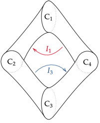
Figure 10: Quadrangle $\mathcal{Q}$

Following [AGG], we introduce the quadrangle of bisectors associated to some of the faithful representations $\rho:G\to\mathrm{\mathrm{PU}}(2,1)$ discussed in Subsection 3.2. We expect quadrangles of bisectors to bound fundamental polyhedra for discrete actions of $G$ on $\mathbb{H}_{\mathbb{C}}^{2}$ and the quotient $\mathbb{H}_{\mathbb{C}}^{2}/G$ to be a disc orbibundle over an orbifold (in our case, a sphere with three cone points). Passing to finite index, one arrives at a complex hyperbolic disc bundle over a closed orientable surface (this comes from the fact that a finitely generated Fuchsian group always has a finite index torsion-free subgroup).

We remind here a few definitions from [AGG].

In order to orient a bisector $B$ we only need to orient its real spine (since the fibers are complex, hence, naturally oriented). An oriented bisector $B$ divides ${\overline{\mathbb{H}}_{\mathbb{C}}^{2}}$ into two half-spaces (closed $4$-balls) $K^{+}$ and $K^{-}$, where $K^{+}$ stands for the half-space lying on the side of the normal vector to $B$.

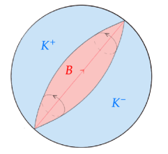
Figure 11: Orienting the real spine fixes a unique orientation of the bisector since the slices are naturally oriented. The half-space $K^{+}$ is the one on the side of the normal vector.

Let $B_{1}=B_{1}[C_{1},C_{2}]$ and $B_{2}=B_{2}[C_{1},C_{3}]$ be two oriented segments of bisectors with a common slice $C_{1}$ such that the corresponding full bisectors are transversal along that slice. The sector from $B_{1}$ to $B_{2}$ is defined to be either $K_{1}^{+}\cap K_{2}^{-}$ (when the oriented angle from $B[C_{1},C_{2}]$ to $B[C_{1},C_{3}]$ at a point $c\in C_{1}$ is smaller than $\pi$) or $K_{1}^{+}\cup K_{2}^{-}$ (when the oriented angle from $B[C_{1},C_{2}]$ to $B[C_{1},C_{3}]$ at a point $c\in C_{1}$ is greater than $\pi$). Note that, while such oriented angle does depend on the point $c$, it cannot equal $\pi$ due to transversality.

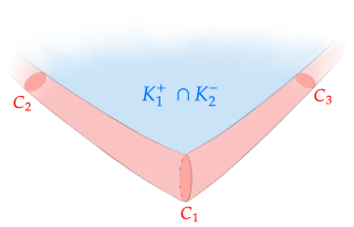
Figure 12: Sector between given by $B_{1}$ and $B_{2}$ when the angle between then is smaller than $\pi$.

Given pairwise ultraparallel complex geodesics $C_{1},C_{2},C_{3}$, the oriented triangle of bisectors $\Delta(C_{1},C_{2},C_{3})$ is simply the union $B[C_{1},C_{2}]\cup B[C_{2},C_{3}]\cup B[C_{3},C_{1}]$ of oriented segments of bisectors. Each such segment is a side of the oriented triangle and each of the complex geodesics $C_{1},C_{2},C_{3}$ is a vertex of the triangle. The triangle is transversal if the full bisectors containing its sides intersect transversally along the common slices.

Given three ultraparallel complex geodesics $C_{1},C_{2},C_{3}$ there are two possible orientations for a triangle of bisectors with vertices $C_{1},C_{2},C_{3}$. Assuming that such a triangle is transversal, its counterclockwise orientation is the one providing an acute oriented angle from $B[C_{3},C_{1}]$ and $B[C_{1},C_{2}]$. By [AGG, Lemma 2.13], this implies that the oriented angles from $B[C_{1},C_{2}]$ to $B[C_{2},C_{3}]$ and from $B[C_{2},C_{3}]$ to $B[C_{3},C_{1}]$ are both acute as well; moreover, in this case, each side of the triangle is contained in the sector determined by the other two.

Let $\Delta(C_{1},C_{2},C_{4})$ and $\Delta(C_{3},C_{4},C_{2})$ be counterclockwise oriented transversal triangles of bisectors sharing a common side. We say these triangles are transversally adjacent if the sector at $C_{1}$ contains a point of $C_{3}$ and the full bisectors containing the segments $B[C_{1},C_{2}]$ and $B[C_{2},C_{3}]$ (respectively, $B[C_{3},C_{4}]$ and $B[C_{4},C_{1}]$) are transversal at $C_{2}$ (respectively, at $C_{4}$). In particular (see [AGG, Lemma 2.14]), this implies that $\Delta(C_{3},C_{4},C_{2})$ is contained in the sector at $C_{1}$; furthermore, $\Delta(C_{3},C_{4},C_{2})$ and $\Delta(C_{1},C_{2},C_{4})$ lie in opposite sides of the full bisector containing $B[C_{2},C_{4}]$.

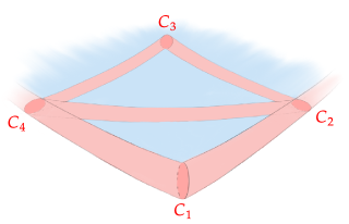
Figure 13: Transversally adjacent triangles.

Let $I_{1},I_{2},I_{3}$ be elliptic isometries as in Subsection 3.2. Let $c_{j},p_{j}\in\mathbb{P}_{\mathbb{C}}(V)$ denote pairwise orthogonal distinct fixed points of $I_{j}$ with $c_{j}\in\mathbb{H}_{\mathbb{C}}^{2}$. In particular, the $p_{j}$’s are positive. We also define the points $c_{4}:=I_{1}^{-1}c_{2}$ and $p_{4}:=I_{1}^{-1}p_{2}$ and the complex geodesics

$$C_{1}:=\mathbb{P}(p_{1})^{\perp}\cap\overline{\mathbb{H}}_{\mathbb{C}}^{2},\qquad C_{2}:=\mathbb{P}(p_{2})^{\perp}\cap\overline{\mathbb{H}}_{\mathbb{C}}^{2},$$

$$C_{3}:=\mathbb{P}(p_{3})^{\perp}\cap\overline{\mathbb{H}}_{\mathbb{C}}^{2},\qquad C_{4}:=\mathbb{P}(p_{4})^{\perp}\cap\overline{\mathbb{H}}_{\mathbb{C}}^{2}.$$

Using the relation $I_{3}I_{2}I_{1}=1$ we obtain $p_{4}=I_{1}^{-1}p_{2}=I_{3}p_{2}$. Therefore $C_{4}=I_{1}^{-1}C_{2}=I_{3}C_{2}$. Note that, by Remark 4, if $C_{1}$ and $C_{2}$ are ultraparallel, $C_{1}\!\!\parallel\!\!C_{2}$, then $C_{1}\!\!\parallel\!\!C_{4}$ since $\mathrm{\mathrm{ta}}(p_{1},p_{2})=\mathrm{\mathrm{ta}}(I_{1}^{-1}p_{1},I_{1}^{-1}p_{2})=\mathrm{\mathrm{ta}}(p_{1},p_{4})>1$. Similarly, $C_{3}\!\!\parallel\!\!C_{2}$ implies $C_{3}\!\!\parallel\!\!C_{4}$. So, if $C_{1}\!\!\parallel\!\!C_{2}$, $C_{3}\!\!\parallel\!\!C_{2}$, and $C_{2}\!\!\parallel\!\!C_{4}$, we get the oriented triangles of bisectors $\Delta(C_{1},C_{2},C_{4})$ and $\Delta(C_{3},C_{4},C_{2})$.

6.2.  Quadrangle conditions

A representation $\rho:G\to\mathrm{\mathrm{PU}}(2,1)$, $g_{j}\mapsto I_{j}$, satisfies the quadrangle conditions if

• $C_{1}\!\!\parallel\!\!C_{2}$, $C_{3}\!\!\parallel\!\!C_{2}$, and $C_{2}\!\!\parallel\!\!C_{4}$.

• The triangles $\Delta(C_{1},C_{2},C_{4}),\Delta(C_{3},C_{4},C_{2})$ are transversal and counterclockwise-oriented.

• The triangles $\Delta(C_{1},C_{2},C_{4}),\Delta(C_{3},C_{4},C_{2})$ are transversally adjacent;

• The oriented angle from $\mathrm{B}[C_{1},C_{4}]$ to $\mathrm{B}[C_{1},C_{2}]$ at $c_{1}$ equals $\displaystyle\frac{2\pi}{n_{1}}$; the oriented angle from $\mathrm{B}[C_{3},C_{2}]$ to $\mathrm{B}[C_{3},C_{4}]$ at $c_{3}$ equals $\displaystyle\frac{2\pi}{n_{3}}$; the sum of the oriented angle from $\mathrm{B}[C_{2},C_{1}]$ to $\mathrm{B}[C_{2},C_{3}]$ at $c_{2}$ with the oriented angle from $\mathrm{B}[C_{4},C_{3}]$ to $\mathrm{B}[C_{4},C_{1}]$ at $c_{4}$ equals $\displaystyle\frac{2\pi}{n_{2}}$.

A representation satisfying the quadrangle conditions give rise to the quadrangle of bisectors

$$\mathcal{Q}:=B[C_{1},C_{2}]\cup B[C_{2},C_{3}]\cup B[C_{3},C_{4}]\cup B[C_{4},C_{1}].$$

The quadrangle $\mathcal{Q}$ bounds polyhedron $Q$ which is on the side of the normal vectors of the oriented segments of bisectors. Indeed, by [AGG, Lemma 2.13], there are no intersections between those segments of bisectors besides the common slices.

6.3.  Discreteness

Let $\rho:G\to\mathrm{\mathrm{PU}}(2,1)$, $g_{j}\mapsto I_{j}$, be a faithful representation satisfying the quadrangle conditions and let $\mathcal{Q}$ be the quadrangle of $\rho$ described in the previous subsection.

Applying [AGr2, Theorem 3.2] we will show that $Q\cap\mathbb{H}_{\mathbb{C}}^{2}$ is a fundamental region for the action of the group $K_{n}$ generated by $I_{1},I_{3}$ with the defining relations $I_{1}^{n_{1}}=I_{3}^{n_{3}}=(I_{3}^{-1}I_{1}^{-1})^{n_{2}}=1$ in $\mathrm{\mathrm{PU}}(2,1)$. The main idea is to prove that, given a point $x$ in the polyhedron $P$, there are corresponding copies of the polyhedron $Q$ that tessellate a (small) ball centered at $x$. When $x$ belongs to the interior of $Q$, the fact is immediate; when it lies in the interior of a side, it follows from the fact that the elliptic isometries $I_{1}$ and $I_{3}$ send the interior of $Q$ to its exterior. Finally, when $x$ is in a vertex, it is enough to understand the case $x=c_{j}$. Here, the tessellation follows from an infinitesimal conditional: the local tessellation of the complex geodesic normal to the vertex at $c_{j}$. For more details, see [AGr2]. This leads to a tessellation of a neighborhood of $Q$ and, by [AGG, Lemma 2.10], such a tessellation provides a tessellation of a metric neighborhood of $Q$. By [AGr2, Theorem 3.2], $K_{n}$ is discrete.

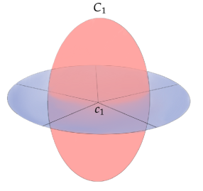
(a)

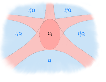
(b)

Figure 14: (a) Tesselation of the complex geodesic normal to $C_{1}$ at $c_{1}$, and (b) tesselation around the vertice $C_{1}$. In both cases, $I_{1}$ has order $5$.

Theorem 20.

The group $K_{n}$ is discrete and $Q$ is a fundamental domain for its action on $\mathbb{H}_{\mathbb{C}}^{2}$.

Proof.

By [AGG, Lemma 2.10], we only need to verify Conditions (i) and (ii) of [AGr2, Theorem 3.2]. Since $I_{1}$ maps $\mathrm{B}[C_{1},C_{4}]$ onto $\mathrm{B}[C_{1},C_{2}]$ and $I_{3}$ maps $\mathrm{B}[C_{3},C_{1}]$ onto $\mathrm{B}[C_{3},C_{4}]$, the Condition (i) of [AGr2, Theorem 3.2] follows from the definition of counterclockwise-oriented transversal triangles. There are three (geometrical) cycles of vertices. The cycle of $C_{1}$ have total angle $2\pi$ at $c_{1}\in C_{1}$ by [AGG, Lemma 3.4]. The same concerns the cycle of $C_{3}$ at $c_{3}\in C_{3}$.

The geometric cycle of $C_{2}$ has length $2n_{2}$ due to the relation $I_{2}^{n_{2}}=1$. Let us verify that the total angle at $c_{2}\in C_{2}$ is $2\pi$. Note that $I_{3}^{-1}$ sends $\mathrm{B}[C_{3},C_{4}]$ onto $\mathrm{B}[C_{3},C_{2}]$ and sends $\mathrm{B}[C_{4},C_{1}]$ onto $\mathrm{B}[C_{2},I_{2}C_{1}]$ (indeed, $I_{3}^{-1}C_{1}=I_{3}^{-1}I_{1}^{-1}C_{1}=I_{2}C_{1}$). Therefore, by the definition of counterclockwise-orientation, the sum of the interior angle from $\mathrm{B}[C_{2},C_{3}]$ to $\mathrm{B}[C_{2},C_{1}]$ at $c_{2}$ with the interior angle from $\mathrm{B}[C_{4},C_{1}]$ to $\mathrm{B}[C_{4},C_{3}]$ at $c_{4}$ equals the angle from $\mathrm{B}[C_{2},C_{3}]$ to $\mathrm{B}[C_{2},I_{2}C_{3}]$ at $c_{2}$. By [AGG, Lemma 3.4], this angle equals $\mathrm{\mathrm{Arg}}(\beta_{1}^{-1}\beta_{2})=2\pi/n_{2}$. ∎

7 Orbifold bundles and Euler number

7.1.  The quadrangle conditions revisited

As in subsection 3.2, let $\rho:G(n_{1},n_{2},n_{3})\to\mathrm{\mathrm{PU}}(2,1)$ be a faithful representation of the turnover group and define $I_{k}:=\rho(g_{k})$. Assume that $I_{1},I_{3}$ are regular elliptic. We choose $I_{k}\in\mathrm{\mathrm{SU}}(2,1)$ as in Remark 9 and fix a negative eigenvector $c_{k}$ of $I_{k}$ as well as a positive one, $p_{k}$. Let $\alpha_{i}$, $\beta_{i}$, $\gamma_{i}^{-1}$, $i=1,2,3$, stand respectively for the eigenvalues of $I_{1}$, $I_{2}$, $I_{3}$ such that

$$I_{1}(c_{1})=\alpha_{1}c_{1},\,I_{2}(c_{2})=\beta_{1}c_{2},\,I_{3}(c_{3})=\gamma_{1}^{-1}c_{3}$$

and

$$I_{1}(p_{1})=\alpha_{2}p_{1},\,I_{2}(p_{2})=\beta_{2}p_{2},\,I_{3}(p_{3})=\gamma_{2}^{-1}p_{3}.$$

Since $\det I_{k}=1$, we must have

$$\alpha_{1}\alpha_{2}\alpha_{3}=\beta_{1}\beta_{2}\beta_{3}=\gamma_{1}\gamma_{2}\gamma_{3}=1.$$

Let us revisit the quadrangle conditions 6.2. This time, we will also formulate such conditions in terms of algebraic formulas that are used both in this section and in section 4.

Define

$$C_{1}=\mathbb{P}(p_{1}^{\perp})\cap\mathbb{H}_{\mathbb{C}}^{2},\quad C_{2}=\mathbb{P}(p_{2}^{\perp})\cap\mathbb{H}_{\mathbb{C}}^{2},\quad C_{3}=\mathbb{P}(p_{3}^{\perp})\cap\mathbb{H}_{\mathbb{C}}^{2}\quad\textrm{ and }\quad C_{4}=I_{1}^{-1}C_{1}\cap\mathbb{H}_{\mathbb{C}}^{2}.$$

Note that, putting $c_{4}:=I_{1}^{-1}c_{2}$ and $p_{4}:=I_{1}^{-1}p_{2}$, we have $C_{4}=\mathbb{P}(p_{4}^{\perp})\cap\mathbb{H}_{\mathbb{C}}^{2}$. Quadrangle condition (Q1) asks that the complex geodesics $C_{1},C_{2},C_{3},C_{4}$ are pairwise ultraparallel:

$$\mathrm{\mathrm{ta}}(p_{1},p_{2})=\mathrm{\mathrm{ta}}(p_{1},p_{4})>1,\quad\mathrm{\mathrm{ta}}(p_{2},p_{3})>1,\quad\textrm{and}\quad\mathrm{\mathrm{ta}}(p_{3},p_{2})=\mathrm{\mathrm{ta}}(p_{3},p_{4})>1$$ (Q1)

(see 4).

Assuming (Q1) we can define the bisectors segments $\mathrm{B}[C_{1},C_{2}]$, $\mathrm{B}[C_{2},C_{3}]$, $\mathrm{B}[C_{2},C_{3}]$, and $\mathrm{B}[C_{3},C_{4}]$.

Condition (Q2) says that the triangles of bisectors $\Delta(C_{1}C_{2}C_{4})$ and $\Delta(C_{2}C_{3}C_{4})$ are transversal and counterclockwise oriented; this is equivalent to the inequalities

$$\epsilon_{0}^{2}t^{2}+s^{2}+t^{2}<1+2t^{2}s\epsilon_{0},\quad\epsilon_{0}^{2}s^{2}+2t^{2}<1+2t^{2}s\epsilon_{0},\quad\epsilon_{1}<0,$$ (Q2)

$$\epsilon_{0}^{\prime 2}t^{\prime 2}+s^{2}+t^{\prime 2}<1+2t^{\prime 2}s\epsilon_{0}^{\prime},\quad\epsilon_{0}^{\prime 2}s^{2}+2t^{\prime 2}<1+2t^{\prime 2}s\epsilon_{0}^{\prime},\quad\epsilon_{1}^{\prime}<0$$

where

$$t_{12}:=\sqrt{\mathrm{\mathrm{ta}}(p_{1},p_{2})},\quad t_{23}:=\sqrt{\mathrm{\mathrm{ta}}(p_{2},p_{4})},\quad t_{31}:=\sqrt{\mathrm{\mathrm{ta}}(p_{4},p_{1})},$$

$$t_{12}^{\prime}:=\sqrt{\mathrm{\mathrm{ta}}(p_{2},p_{3})},\quad t_{23}^{\prime}:=\sqrt{\mathrm{\mathrm{ta}}(p_{3},p_{4})},\quad t_{31}:=\sqrt{\mathrm{\mathrm{ta}}(p_{4},p_{2})},$$

$$\epsilon_{0}+\epsilon_{1}i:=\frac{\sigma}{|\sigma|},\quad\textrm{where}\quad\sigma:=\langle p_{1},p_{2}\rangle\langle p_{2},p_{4}\rangle\langle p_{4},p_{1}\rangle,$$

$$\epsilon_{0}^{\prime}+\epsilon_{1}^{\prime}i:=\frac{\sigma^{\prime}}{|\sigma^{\prime}|},\quad\textrm{where}\quad\sigma^{\prime}:=\langle p_{2},p_{3}\rangle\langle p_{3},p_{4}\rangle\langle p_{4},p_{2}\rangle$$

(see [AGG, Criterion 2.27]). Note that $t_{12}=t_{31}$, $t_{12}^{\prime}=t_{23}^{\prime}$, and $t_{23}=t_{31}^{\prime}$. We write $t:=t_{12}$, $t^{\prime}=t_{12}^{\prime}$ and $s=t_{23}$.

The quadrangle condition (Q3) asserts that the triangles $\Delta(C_{1},C_{2},C_{4})$ and $\Delta(C_{3},C_{4},C_{2})$ are transversally adjacent. It is guaranteed by the conditions (Q3.1), (Q3.2), (Q3.3) below. Condition (Q3.1) concerns the transversality of the bisectors $B[C_{1},C_{2}]$ and $B[C_{2},C_{3}]$,

$$\left|\left(\frac{\langle p_{3},p_{1}\rangle\langle p_{2},p_{2}\rangle}{\langle p_{3},p_{2}\rangle\langle p_{2},p_{1}\rangle}\right)-1\right|<\sqrt{1-\frac{1}{\mathrm{\mathrm{ta}}(p_{2},p_{3})}}\sqrt{1-\frac{1}{\mathrm{\mathrm{ta}}(p_{2},p_{1})}}.$$ (Q3.1)

(see [AGG, Criterion 3.3]). Similarly, (Q3.2) states the transversality of the bisectors $B[C_{1},C_{4}]$ and $B[C_{4},C_{3}]$,

$$\left|\left(\frac{\langle p_{1},p_{3}\rangle\langle p_{4},p_{4}\rangle}{\langle p_{1},p_{4}\rangle\langle p_{4},p_{3}\rangle}\right)-1\right|<\sqrt{1-\frac{1}{\mathrm{\mathrm{ta}}(p_{4},p_{1})}}\sqrt{1-\frac{1}{\mathrm{\mathrm{ta}}(p_{4},p_{3})}}.$$ (Q3.2)

Finally, (Q3.3) implies that $c_{3}$ belongs to the interior of the sector at $C_{1}$ of the triangle $\Delta(C_{1},C_{2},C_{4})$:

$$\mathrm{\mathrm{Im}}\left(\frac{\langle p_{1},c_{3}\rangle\langle c_{3},p_{2}\rangle}{\langle p_{1},p_{2}\rangle}\right)\geq 0\quad\textrm{and}\quad\mathrm{\mathrm{Im}}\left(\frac{\langle p_{4},c_{3}\rangle\langle c_{3},p_{1}\rangle}{\langle p_{4},p_{1}\rangle}\right)\geq 0$$ (Q3.3)

(see [AGG, Lemma 3.5]).

Consider the polyhedron $Q$ bounded in $\mathbb{H}_{\mathbb{C}}^{2}$ by the quadrangle

$$\mathcal{Q}:=\big{(}B[C_{1},C_{2}],B[C_{2},C_{3}],B[C_{3},C_{4}],B[C_{4},C_{1}]\big{)}.$$

It follows from [AGG, Lemma 3.4] that condition (Q4) translates, in terms of the eigenvalues $\alpha_{i},\beta_{i},\gamma_{i}$, into

$$\alpha_{2}/\alpha_{1}=\exp(-2\pi i/n_{1}),\quad\beta_{2}/\beta_{1}=\exp(-2\pi i/n_{2}),\quad(\gamma_{2}/\gamma_{1})^{-1}=\exp(-2\pi i/n_{3})$$ (Q4)

7.2.  Deformation lemma

Given a complex geodesic $C$ with a chosen $c\in C$, we identify $C$ with the unit open disc in $\mathbb{C}$ as follows. Let $p$ be the point orthogonal to $c$ in the complex projective line extending $C$. Take representatives such that $-\langle c,c\rangle=\langle p,p\rangle=1$. Then every point in $C$ has the form $c+\gamma p$, $|\gamma|\leq 1$. For obvious reasons, we call $c$ the center of $C$.

Consider the action of $\mathbb{S}^{1}$ on the circle $\partial_{\infty}C$ by rotations centered at $c$. More precisely, given a unit complex number $\theta\in\mathbb{S}^{1}$, we define

$$\gamma[c+\theta p]=[c+\gamma\theta p].$$

In particular, we have an $\mathbb{S}^{1}$-action on the vertices $C_{i}$ of the quadrangle $\mathcal{Q}$, where each $C_{i}$ has center $c_{i}$.

Lemma 21.

Consider an orientation on $V$ and let $q_{i}$ be a vector such that $c_{i},p_{i},q_{i}$ is a positively oriented orthonormal basis of $V$. There is a family of curves $c_{i}(\delta),p_{i}(\delta),q_{i}(\delta)$, with $\delta\in[0,1]$, such that

• $c_{i}(0)=c_{i}$, $p_{i}(0)=p_{i}$ and $q_{i}(0)=q_{i}$;

• for each $\delta$ the vectors $c_{i}(\delta),p_{i}(\delta),q_{i}(\delta)$ form a positively oriented orthonormal basis of $V$;

• for all $i,j$, with $i\neq j$, we have $\mathrm{\mathrm{ta}}(p_{i}(\delta),p_{j}(\delta))>1$;

• If $C_{i}(\delta):=\mathbb{P}(p_{i}(\delta)^{\perp})$ and we consider the triangles of bisectors $\triangle_{1}(\delta)$, with vertices $C_{1}(\delta)$, $C_{2}(\delta)$ and $C_{4}(\delta)$, and $\triangle_{2}(\delta)$, with vertices $C_{2}(\delta)$, $C_{3}(\delta)$ and $C_{4}(\delta)$, then for each $\delta$ the triangles $\triangle_{1}(\delta)$ and $\triangle_{2}(\delta)$ are transversal and counter-clockwise oriented.

• $q_{1}(1)=q_{2}(1)=q_{3}(1)=q_{4}(1)$.

The last item means that if $\mathcal{Q}(\delta)$ is the quadrangle with vertices $C_{i}(\delta)$, then the bisectors forming the boundary of $\mathcal{Q}(1)$ all have the same focus.

Proof: Consider $s,t,t^{\prime},\epsilon_{0},\epsilon_{0}^{\prime}$ as consider in the inequalities (Q2). It is know from lemma $\mathbf{A.31}$ in [AGG] that the parameters $s,t,\epsilon_{0}$, with $t,s>1$ and $0<\epsilon_{0}<1$, determine up to isometry the transversal counter-clockwise oriented triangle of bisectors $\triangle_{1}:=\triangle[C_{1},C_{2},C_{4}]$.

Suppose $t>s$. We will show that choosing a convenient $\epsilon_{0}>0$ we can reduce $t$ until $t=s$. The inequalities which determine that $\triangle_{1}$ is transversal are the

$$\epsilon_{0}^{2}s^{2}+2t^{2}<1+2\epsilon_{0}st^{2}\leq 2t^{2}+s^{2}.$$

Consider the quadratic polynomial $f(x)=x^{2}s^{2}-2xst^{2}+2t^{2}-1$. The roots of $f(x)=0$ are

$$x=\frac{t^{2}\pm(t^{2}-1)}{s}$$

and, therefore, $f(x)<0$ when $1/s<x<(2t^{2}-1)/s$. Notice $x_{0}=(2s^{2}-1)/s$ is between $1/s$ and $(2t^{2}-1)/s$. We can reduce $\epsilon_{0}$ until $1/s<\epsilon_{0}<x_{0}$. Now, since the inequality $\epsilon_{0}^{2}s^{2}+2t^{2}<1+2\epsilon_{0}st^{2}$ is equivalent

$$t^{2}>\frac{s\epsilon_{0}+1}{2},$$

and, by our choice of $\epsilon_{0}$,

$$s^{2}>\frac{s\epsilon_{0}+1}{2},$$

we can reduce $t$ until $t=s$.

Note that the inequality $1+2\epsilon_{0}st^{2}\leq s^{2}+2t^{2}$ is kept during the above procedure.

Applying the same reasoning to $t^{\prime}$ we may suppose $1<t,t^{\prime}\leq s$.

Now, we will show that we can deform $t$ and $\epsilon_{0}$ until $t=s$ and $1+2\epsilon_{0}s^{3}=3s^{2}$ always keeping $1<t\leq s$, $0<\epsilon_{0}<1$ and $\epsilon_{0}^{2}t^{2}+s^{2}+t^{2}<1+2\epsilon_{0}st^{2}$.

Indeed, if $t<s$, then increase $t$ until one of the two following possibilities happens:

$$t=s\quad\textrm{or}\quad 1+2\epsilon_{0}st^{2}=2t^{2}+s^{2}.$$

If $t=s$, then we have $1+2\epsilon_{0}s^{3}\leq 3s^{2}$, which is equivalent to

$$\epsilon_{0}\leq\frac{3s^{2}-1}{2s^{3}}.$$

Now, the function $g(x):=\frac{3x^{2}-1}{2x^{3}}$ is strictly decreasing for $x>1$ and, therefore, $g(x)<g(1)=1$ for $x>1$. Therefore, we can increase $\epsilon_{0}$ until

$$\epsilon_{0}=\frac{3s^{2}-1}{2s^{3}},$$

or equivalently $1+2\epsilon_{0}s^{3}=3s^{2}$.

If $1<t\leq s$ and $1+2\epsilon_{0}st^{2}=2t^{2}+s^{2}$, with $0<\epsilon_{0}<1$, then we have the inequality

$$2t^{2}+s^{2}<2st^{2}+1,$$

or equivalently

$$t^{2}>\frac{s^{2}-1}{2(s-1)}=\frac{s+1}{2}.$$

Therefore, we can increase $t$ until $t=s$ and have $\epsilon_{0}\in(0,1)$ satisfying $1+2\epsilon_{0}s^{3}=3s^{2}$.

So, we can deform $t$ and $\epsilon_{0}$, always keeping $t>1$ and $0<\epsilon_{0}<1$ during the process, and in the end we obtain $t=s$ and $1+2\epsilon_{0}s^{3}=3s^{2}$.

By the same reasoning we can deform $t^{\prime}$ and $\epsilon_{0}^{\prime}$ such that we always have $t^{\prime}>1$ and $0<\epsilon_{0}^{\prime}<1$ during the deformation and in the end we obtain $t^{\prime}=s$ and $1+2\epsilon_{0}^{\prime}s^{3}=3s^{2}$.

So we reduced the problem to the case where $t=t^{\prime}=s$ and $\epsilon_{0}=\epsilon_{0}^{\prime}$. Geometrically we deformed the quadrangle $P$ inside $\mathbb{H}_{\mathbb{C}}^{2}$ always keeping the vertices $C_{2}$ and $C_{4}$ fixed and moving $C_{1}$ and $C_{3}$ around such that the two triangles of bisectors are kept transversal and counter-clockwise oriented. In the case we are now all sides of the quadrangle have the same length.

Now, the quadrangle $P$ depends only on the parameters $s$ and $\epsilon_{0}$, which means it depends only on the triangle $\triangle_{1}$. Let $q$ be the focus of the bisector $\mathrm{B}[C_{2},C_{4}]$. Using that the space of transversal and counter-clockwise oriented triangles of bisectors is path-connected [AGG, Lemma 2.28] we can deform $\triangle_{1}$ until $q_{1}=q_{2}=q_{3}=q$. The same deformation will be done to the triangle $\triangle_{2}=\triangle[C_{2},C_{3},C_{4}]$ simultaneously using the same parameters of $\triangle_{1}$. Therefore, in the end of the deformation we have the desired quadrangle. ∎

Now we apply lemma 21 to the quadrangle $\mathcal{Q}$. Deform the vertices $C_{1},C_{2},C_{3},C_{4}$ until the focuses of the four bisectors coincide in one point $q\in\mathrm{E}(V)$. Let $C_{1}^{\prime},C_{2}^{\prime},C_{3}^{\prime},C_{4}^{\prime}$ stand for the vertices at the end of the deformation. We can assume that the deformation is such that the centers $c_{1},c_{2},c_{3},c_{4}$ belong to $\mathbb{P}(q^{\perp})\cap\mathbb{H}_{\mathbb{C}}^{2}$ at the end and are the vertices $c_{1}^{\prime},c_{2}^{\prime},c_{3}^{\prime},c_{4}^{\prime}$ of a convex quadrilateral $P$. Also, we can suppose that the angles at $c_{1}^{\prime},c_{2}^{\prime},c_{3}^{\prime},c_{4}^{\prime}$ are respectively $2\pi/n_{1},\pi/n_{2},2\pi/n_{3},\pi/n_{2}$, that is, this quadrilateral constitutes a fundamental polygon for the turnover group $\langle R_{1},R_{2},R_{3}\rangle$ action on the hyperbolic plane $\mathbb{P}(q^{\perp})\cap\mathbb{H}_{\mathbb{C}}^{2}$; here, $R_{1},R_{2},R_{3}$ are rotations in $\mathbb{P}(q^{\perp})\cap\mathbb{H}_{\mathbb{C}}^{2}$ with respective centers $c_{1}^{\prime},c_{2}^{\prime},c_{3}^{\prime}$ and angles $-2\pi/n_{1},-2\pi/n_{2},-2\pi/n_{3}$ and satisfying the relation $R_{3}R_{2}R_{1}=1$.

We have a polyhedron $Q^{\prime}$ bounded in $\mathbb{H}_{\mathbb{C}}^{2}$ by the quadrangle

$$\mathcal{Q}^{\prime}:=(\mathrm{B}[C_{1}^{\prime},C_{2}^{\prime}],\mathrm{B}[C_{2}^{\prime},C_{3}^{\prime}],\mathrm{B}[C_{3}^{\prime},C_{4}^{\prime}],\mathrm{B}[C_{4}^{\prime},C_{1}^{\prime}]).$$

The deformation gives rise to a diffeomorphism

$$F:Q^{\prime}\to Q$$

such that the restriction $F|_{\mathcal{Q}^{\prime}}:\mathcal{Q}^{\prime}\to\mathcal{Q}$ maps slices to slices isometrically. Furthermore, we can assume that the geodesic curves $G[c_{i}^{\prime},c_{i+1}^{\prime}]$ are mapped by this diffeomorphism to curves $g_{i}$ with end points $c_{i}$ and $c_{i+1}$ such that $I_{1}g_{4}=g_{1}$ and $I_{3}g_{2}=g_{3}$. The curve $g_{1}\cup g_{2}\cup g_{3}\cup g_{4}$ intersects each slice of $\mathcal{Q}$ in one point, which we will take as a center. Given these centers, we introduce an $\mathbb{S}^{1}$-action on each slice of $\mathcal{Q}$ such that the map $F$ restricted to $\mathcal{Q}^{\prime}$ is $\mathbb{S}^{1}$-equivariant.

Note that there are two ways of mapping $B[C_{1}^{\prime},C_{2}^{\prime}]$ to $B[C_{4},C_{1}]$. The first one is by the map

$$[x+\gamma q]\mapsto I_{1}^{-1}F(x+\gamma q)$$

and the second one is

$$[x+\gamma q]\mapsto F(R^{-1}x+(\alpha_{3}/\alpha_{1})\gamma q),$$

and since the diffeomorphism $F$ maps slices to slices isometrically we have this two maps coincide in $C_{1}^{\prime}$. Nevertheless, we want these two maps to be equal near $C^{\prime}_{1}$ in order to calculate the Euler number of the disc orbibundle over $\mathbb{S}^{2}(n_{1},n_{2},n_{3})$ to be constructed, and the lemma bellow tell us that this is possible. The proof of this lemma is based on the idea of “twisting the tube”. More visually, we have the diffeomorphism $G:B[C_{1}^{\prime},C_{2}^{\prime}]\to B[C_{1}^{\prime},C_{2}^{\prime}]$ given by $[x+\gamma q]\mapsto F^{-1}I_{1}F(R^{-1}x+(\alpha_{3}/\alpha_{1})\gamma q)$ and it gives us the behavior described in the figure 15.

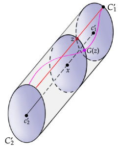
Figure 15: Consider the red curve intersecting each slice of the bisector $B[C^{\prime}_{1},C^{\prime}_{2}]$ once. If $z$ is in this red curve, then it can be writen as $z=x+\gamma q$, where $x$ is a representative of the center of the disc containing $z$ and satisfying $\langle x,x\rangle=-1$, and $G(z)$ will be a rotation depending on the center $x$. Therefore, for $x$ near $c_{1}^{\prime}$ we have $G(x+\gamma q)=\big{[}x+\exp(i\theta(x))\gamma q\big{]}$, with $\theta(c_{1}^{\prime})=0$.

We want the red and the pink curve to coincide near $C^{\prime}_{1}$.

Lemma 22.

We can modify the diffeomorphism $F:\mathcal{Q^{\prime}}\to\mathcal{Q}$ in such a way it still maps slices to slices isometrically and

$$F(x+\gamma q)=I_{1}F(R_{1}^{-1}x+(\alpha_{3}/\alpha_{1})^{-1}\gamma q)\quad\textrm{for}\quad x\in N_{1}\cap\mathrm{\mathrm{G}}[c_{1}^{\prime},c_{2}^{\prime}],\quad\langle x,x\rangle=-1,$$

for some neighborhood $N_{1}$ of $c_{1}^{\prime}$ in $\mathbb{P}(q^{\perp})$.

Proof: On the vertices we have

$$\gamma F(c_{i}^{\prime}+\theta q)=F(c_{i}^{\prime}+\gamma\theta q),$$

and therefore the desired identity holds on $c_{1}^{\prime}$.

By continuity, for a small neighborhood $V$ of $c_{1}^{\prime}$ on the geodesic $\mathrm{\mathrm{G}}[c_{1}^{\prime},c_{2}^{\prime}]$ we have a smooth function $\theta:V\to\mathbb{R}$ satisfying

$$F^{-1}I_{1}F\big{(}R_{1}^{-1}x+(\alpha_{3}/\alpha_{1})^{-1}\gamma q\big{)}=\big{[}x+\exp(i\theta(x))\gamma q\big{]}\quad\textrm{for}\quad x\in V\cap\mathrm{\mathrm{G}}[c_{1}^{\prime},c_{2}^{\prime}],\quad\langle x,x\rangle=-1.$$

In particular, we may suppose $\theta(c_{1}^{\prime})=0$.

There is $\widetilde{\theta}$ in $\mathrm{\mathrm{G}}[c_{1},c_{2}]$ such that $\theta(x)=\widetilde{\theta}(x)$ in a small compact neighborhood $N_{1}\subset V$ of $c_{1}^{\prime}$ such that $\mathrm{supp}(\widetilde{\theta})\subset V$. Furthermore, we can extend $\widetilde{\theta}$ to all the quadrilateral $P$ in such a way that $\widetilde{\theta}$ is zero over the geodesics $\mathrm{\mathrm{G}}[c_{2}^{\prime},c_{3}^{\prime}]$, $\mathrm{\mathrm{G}}[c_{3}^{\prime},c_{4}^{\prime}]$, and $\mathrm{\mathrm{G}}[c_{4}^{\prime},c_{1}^{\prime}]$. Therefore, we can consider $\widehat{F}(x+\gamma q)=F\Big{(}x+\exp\big{(}i\widetilde{\theta}(x)\big{)}\gamma q\Big{)}$, with $\langle x,x\rangle=-1$. With this new map we have

$$\widehat{F}(x+\gamma q)=I_{1}\widehat{F}\big{(}R_{1}^{-1}x+(\alpha_{3}/\alpha_{1})^{-1}\gamma q\big{)}\quad\textrm{for}\quad x\in N_{1}\cap\mathrm{\mathrm{G}}[c_{1}^{\prime},c_{2}^{\prime}],\quad\langle x,x\rangle=-1,$$

where we are using $\widetilde{\theta}(R^{-1}x)=0$ because $R_{1}^{-1}x\in G[c_{4}^{\prime},c_{1}^{\prime}]$. ∎

We may also suppose the same kind of property for the other vertices: For $i=2,3,4$ we have a small neighborhood $N_{i}$ of the point $c_{i}^{\prime}$ in $\mathbb{P}(q^{\perp})$ such that

$$F(x+\gamma q)=I_{3}^{-1}F\big{(}R_{3}x+(\beta_{3}/\beta_{1})\gamma q\big{)} \quad x\in N_{2}\cap\mathrm{\mathrm{G}}[c_{2}^{\prime},c_{3}^{\prime}],\quad\langle x,x\rangle=-1,$$ for

$$F(x+\gamma q)=I_{3}F\big{(}R_{3}^{-1}x+(\gamma_{3}/\gamma_{1})\gamma q\big{)} \quad x\in N_{3}\cap\mathrm{\mathrm{G}}[c_{3}^{\prime},c_{4}^{\prime}],\quad\langle x,x\rangle=-1,$$ for

$$F(x+\gamma q)=I_{1}^{-1}F\big{(}R_{1}x+\gamma q\big{)} \quad x\in N_{4}\cap\mathrm{\mathrm{G}}[c_{4}^{\prime},c_{1}^{\prime}],\quad\langle x,x\rangle=-1.$$ for

7.3.  Constructing complex hyperbolic disc orbigoodles over $\mathbb{S}^{2}(n_{1},n_{2},n_{3})$

An $n$-orbifold $B$ is a space locally modeled by quotients of the form $\mathbb{D}^{n}/\Gamma$, where $\Gamma$ is a finite subgroup of $\mathrm{O}(n)$. All orbifolds considered in this paper are locally oriented, which means that we are only considering trivializations with $\Gamma\subset\mathrm{SO}(n)$. More technically by space we mean diffeological space (for details see [Bot1]). A diffeomorphism $\phi:\mathbb{D}^{n}/\Gamma\to D$, where $D$ stands for an open subset of $B$, is called orbifold chart. Furtheremore, if $\phi([0])=p$ we say that the orbifold chart is centered at $p$. We say that $p$ is a regular point if the finite group $\Gamma$ corresponding to a chart centered at $p$ is trivial, that is, the orbifold is locally Euclidian around $p$; the point is called singular otherwise and the order of the singular point is the cardinality of the group $\gamma$. Since we are interested in orbibundles over $2$-orbifolds, the groups $\Gamma^{\prime}s$ are generated by $\exp(2\pi i/n)$, where we think of $\mathbb{D}^{2}$ as the unit open ball on the complex plane.

Definition 23.

(see [Bot1, 3.1. Orbibundles]) Consider a smooth map between orbifolds $\zeta:L\to B$. We say $\zeta$ is a disc orbibundle for every point $p\in B$ there is an orbifold chart $\phi:\mathbb{D}^{n}/\Gamma\to D$ centered at $p$ satisfying the following properties:

• there is a smooth action of $\Gamma$ on $\mathbb{D}^{n}\times\mathbb{D}^{2}$ of the form $h(x,f)=(hx,a(h,x)f)$, where$a:\Gamma\times\mathbb{D}^{n}\to\mathrm{Diff}(\mathbb{D}^{2})$ is smooth and $\mathrm{Diff}(\mathbb{D}^{2})$ stands for the group of diffeomorphisms of $\mathbb{D}^{2}$;

• there is a diffeomorphism $\Phi:(\mathbb{D}^{n}\times\mathbb{D}^{2})/\Gamma\to\zeta^{-1}(D)$ such that the diagram

  (24)

  commutes, where $\mathrm{pr}_{1}([x,f])=[x]$.

A disc orbigoodle (see [Bot1, Definition 23]) is a special case of disc orbibundle. Consider a simply-connected manifold $\mathbb{H}$ on which acts a group $G$ properly discontinuously. If we have an action of $G$ on $\mathbb{H}\times\mathbb{D}^{2}$ by diffeomorphisms of the form $g(p,v)=(gp,a(g,p)v)$ then the quotient $(\mathbb{H}\times\mathbb{D}^{2})/G\to\mathbb{H}/G$ is a disc orbibundle. Such orbibundles are called disc orbigoodles. All disc orbibundles of this paper are disc orbigoodles where $\mathbb{H}$ is the hyperbolic plane.

A natural $\mathbb{S}^{1}$-action is defined on $Q^{\prime}$ (the polyhedron $Q^{\prime}$ is defined right after Lemma 21) because

$$Q^{\prime}=\bigcup_{x\in P}\big{(}\mathrm{L}[q,x]\cap\mathbb{H}_{\mathbb{C}}^{2}\big{)},$$

where $\mathrm{L}[q,x]$ is the complex projective line connecting $q$ and $x$, and each disc $\overline{\mathbb{H}_{\mathbb{C}}^{2}}\cap\mathrm{L}[q,x]$ has the point $x$ as center. The action we define is simply given by rotation around $x$,

$$\gamma[x+\theta q]=[x+\gamma\theta q],$$

where $\langle x,x\rangle=-1$, $\gamma\in\mathbb{S}^{1}$, and $|\theta|\leq 1$. Therefore, we can define an $\mathbb{S}^{1}$-action on $Q$ using the diffeomorphism $F$. Since $F$ is an isometry at the level of the discs foliating the quadrangles $\mathcal{Q}^{\prime},\mathcal{Q}$, $I_{1}g_{4}=g_{1}$ and $I_{3}g_{2}=g_{3}$ (remind that the curves $g_{i}$’s are image under $F$ of the curves defining the boundary of the quadrilateral $P$), we conclude

$$\gamma I_{1}F(x)=I_{1}\gamma F(x)\quad\text{for}\quad x\in B[C_{1}^{\prime},C_{4}^{\prime}],$$

$$\gamma I_{3}F(x)=I_{3}\gamma F(x)\quad\text{for}\quad x\in B[C_{2}^{\prime},C_{3}^{\prime}],$$

$\gamma\in\mathbb{S}^{1}$. In particular, since $F(c_{i}^{\prime})=c_{i}$ for each vertex $C_{i}=F(C_{i}^{\prime})$, we obtain that $F(\gamma x)$ is the rotation of $F(x)$ with respect to the center $c_{i}$ of $C_{i}$ and angle given by the unitary complex number $\gamma$.

Note that the image of the quadrilateral $P$ under $F$ in addition to the action of $G$ on $\mathbb{H}_{\mathbb{C}}^{2}$ provides an embedded disc $D$ transversal to all discs foliating $\mathbb{H}_{\mathbb{C}}^{2}$ and stable under action of $\mathbb{S}^{1}$. Hence, the quotient $L:=\mathbb{H}_{\mathbb{C}}^{2}/G\to D/G$ is a disc orbigoodle and by construction $D/G=\mathbb{S}^{2}(n_{1},n_{2},n_{3})$.

Furthermore, from $\partial_{\infty}Q$ we can build the $\mathbb{S}^{1}$-orbibundle $\mathbb{S}^{1}(L)\to D/G$, from which we will deduce the formula for the Euler number of the disc bundle $L\to D/G$. Let $\pi:\partial_{\infty}Q\to\mathbb{S}^{1}(L)$ be the quotient map. It is interesting to note that the action on $\partial L$ is not necessarily principal, i.e., there are points $x\in\partial_{\infty}Q$ such that the map $\mathbb{S}^{1}\ni\gamma\mapsto\pi(\gamma x)\in\mathbb{S}^{1}(L)$ is non-injective. More precisely, the action fails to be principal on the circles $\pi(\partial C_{j})$’s.

Take a small ball $V_{i}$ of radius $r$ and center $c_{i}^{\prime}$ on $P$ for $i=1,2,3,4$. Let’s see what happens nearby these non-principal circles. Without loss of generality, we will work with $i=1$. We have the open set

$$U:=F\left[\bigcup_{x\in V_{1}}\mathrm{L}(x,q)\cap\partial\mathbb{H}_{\mathbb{C}}^{2}\right]$$

of $\partial_{\infty}Q$ and the open set $W:=\pi(U)$ in $\mathbb{S}^{1}(L)$. Let $p^{\prime}_{1}$ be the orthogonal point $c^{\prime}_{1}$ on the projective line $\mathbb{P}(q^{\perp})$ such that $\langle p^{\prime}_{1},p^{\prime}_{1}\rangle=1$, $c^{\prime}_{2}\in\mathbb{R}c^{\prime}_{1}+\mathbb{R}p^{\prime}_{1}$ and the geodesic curve $t\mapsto[\cosh(t)c^{\prime}_{1}+\sinh(t)p^{\prime}_{1}]$ reaches $c^{\prime}_{2}$ for some $t>0$, that is, this curve goes from $c^{\prime}_{1}$ to $c^{\prime}_{2}$.

Consider the map $\Lambda:\mathbb{S}^{1}\times S\to W$ given by

$$\Lambda(\gamma,z)=\pi\circ F\left[\frac{c_{1}^{\prime}+zp_{1}^{\prime}}{\sqrt{1-|z|^{2}}}+\gamma q\right],$$

where $S$ is the intersection of $\overline{\mathbb{D}_{\epsilon}^{2}}\subset\mathbb{C}$, the disc of center $0$ and radius $\epsilon$ such that $\cosh(r)=1/\sqrt{1-\epsilon^{2}}$, and the sector given by the inequality $0\leq\arg(z)\leq 2\pi/n_{1}$. The sides of $S$ can be glued because, if $z$ is real, $\Lambda(\gamma,z)=\Lambda(\gamma,\xi z)$, where $\xi=\exp(2\pi/n_{1})$. Therefore, we have the smooth map

$$\Lambda:\mathbb{S}^{1}\times\big{(}\overline{\mathbb{D}_{\epsilon}^{2}}/\langle\xi\rangle\big{)}\to W,$$

and using the natural projection $\overline{\mathbb{D}_{\epsilon}^{2}}\to\overline{\mathbb{D}_{\epsilon}^{2}}/\langle\xi\rangle$, we have the smooth map

$$\widetilde{\Lambda}:\mathbb{S}^{1}\times\overline{\mathbb{D}_{\epsilon}^{2}}\to W.$$

Remember the eigenvalues of $I_{1}$ are $\alpha_{1}$, $\alpha_{2}$ and $\alpha_{3}$. Let $e^{2\pi il_{1}/n_{1}}=\alpha_{3}/\alpha_{1}$ and $e^{-2\pi i/n_{1}}=\alpha_{2}/\alpha_{1}$, with $0\leq l_{1}<n_{1}$.

Taking the diffeomorphism $\eta(\gamma,z):=(\xi^{l_{1}}\gamma,\xi^{-1}z)$ on $\mathbb{S}^{1}\times\overline{\mathbb{D}_{\epsilon}^{2}}$, we have the equivariant diffeomorphism

$$\widehat{\Lambda}:\big{(}\mathbb{S}^{1}\times\overline{\mathbb{D}_{\epsilon}^{2}}\big{)}/\langle\eta\rangle\to W$$

as a consequence of lemma 22. So $W$ is a solid torus (see [Bot1, Lemma 20]) with an $\mathbb{S}^{1}$ action which is principal except for the circle $\big{(}\mathbb{S}^{1}\times 0\big{)}/\langle\eta\rangle$. Hence we have a trivialization of the $\mathbb{S}^{1}$-orbibundle around the fiber $\pi(\partial_{\infty}C_{1})$.

If we write $\beta_{3}/\beta_{1}=e^{2\pi il_{2}/n_{2}}$ and $\gamma_{3}/\gamma_{1}=e^{2\pi il_{3}/n_{3}}$, with $1\leq l_{1}<n_{i}$, we obtain the same kind of trivialization of the $\mathbb{S}^{1}$-orbibundle as described above for $\pi(\partial_{\infty}C_{2})$ and $\pi(\partial_{\infty}C_{3})$.

7.4.  An integer contribution to the Euler number

We now tackle the problem of calculating the Euler number of the constructed orbibundles. First, we need to introduce a particular curve $d$ for the quadrangle $\mathcal{Q}$.

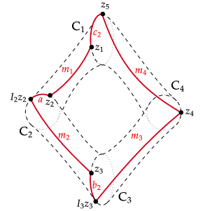
Figure 16: Meridional curve.

Take a point $z_{1}$ on $\partial_{\infty}C_{1}$ and define the following curves:

$\bullet$ the meridional curve $m_{1}\subset\partial_{\infty}\mathrm{B}[C_{1},C_{2}]$ that begins at $z_{1}\in\partial_{\infty}C_{1}$ and ends at $z_{2}\in\partial_{\infty}C_{2}$;

$\bullet$ the naturally oriented simple arc $a\subset\partial_{\infty}C_{2}$ that begins at $z_{2}$ and ends at $I_{2}z_{2}$;

$\bullet$ the meridional curve $m_{2}\subset\partial_{\infty}\mathrm{B}[C_{2},C_{3}]$ that begins at $I_{2}z_{2}$ and ends at $z_{3}\in\partial_{\infty}C_{3}$;

$\bullet$ the naturally oriented simple arc $b_{2}\subset\partial_{\infty}S$ that begins at $z_{3}$ and ends at $I_{3}z_{3}$;

$\bullet$ the meridional curve $m_{3}\subset\partial_{\infty}\mathrm{B}[C_{3},C_{4}]$ that begins at $I_{3}z_{3}$ and ends at $z_{4}\in\partial_{\infty}C_{4}$;

$\bullet$ the meridional curve $m_{4}\subset\partial_{\infty}\mathrm{B}[C_{4},C_{1}]$ that begins at $z_{4}$ and ends at $z_{5}\in\partial_{\infty}C_{1}$;

$\bullet$ the naturally oriented simple arc $c_{2}\subset\partial_{\infty}C_{1}$ that begins at $z_{5}$ and ends at $z_{1}$.

Note that $z_{4}=I_{3}I_{2}z_{2}$, because $I_{3}m_{2}=m_{3}$. Therefore, $z_{4}=I_{1}^{-1}z_{2}$ and consequently $z_{5}=I_{1}^{-1}z_{1}$.

Let

$$d:=m_{1}\cup a\cup m_{2}\cup b_{2}\cup m_{3}\cup m_{4}\cup c_{2}$$ (25)

and let $s$ stand for a generator of $H_{1}(\partial_{\infty}Q,\mathbb{Z})$. Then there exists $f\in\mathbb{Z}$ such that $d=fs$ in $H_{1}(\partial_{\infty}Q,\mathbb{Z})$. This integer $f$ is an important component of the Euler number of the orbibundles we will encounter in subsection 7.5. It will be expressed in a more computational friendly manner in subsection 7.6.

7.5.  Euler Number of the constructed disc bundles

Following [Bot1, 3.2. Euler number of $\mathbb{S}^{1}$-orbibundles over $2$-orbifolds] the Euler number of the disc orbibundle $L\to D/G$ described in the subsection 7.3 is the Euler number of the $\mathbb{S}^{1}$-orbibundle $\mathbb{S}^{1}(L)\to D/G$.

In general, if $M\to B$ is an $\mathbb{S}^{1}$-orbibundle over a oriented compact connected $2$-orbifold with singular points $x_{1},\ldots,x_{n}$ then the Euler number is calculated as follows: Take a regular point $x_{0}$ and for each $i=0,\cdots,n$ consider a small smooth closed disc $D_{i}$ centered at $x_{i}$ trivializing the $\mathbb{S}^{1}$-orbibundle $M\to B$. The $\mathbb{S}^{1}$-orbibundle restricted over the surface with boundary $B^{\prime}=B\setminus\sqcup_{i}D_{i}$ is trivial, since $\mathbb{S}^{1}$-bundles over graphs are trivial and $B^{\prime}$ is homotopically equivalent to a graph. Consider a section $\sigma$ for $M|_{B}^{\prime}\to B^{\prime}$ and a fiber $s$ over a regular point, oriented accordingly to action of $\mathbb{S}^{1}$ on $M$. The Euler number of the $\mathbb{S}^{1}$-orbibundle $M\to B$ is defined by the identity

$$\sigma|_{\partial B^{\prime}}=-e(M)s$$

in $H_{1}(M,\mathbb{Q})$ (See [Bot1, Definition 16]).

Now we apply the above definition of Euler number to the particular bundle $\mathbb{S}^{1}(L)\to D/G$. Let us also denote $\mathbb{S}^{1}(L)$ by $M$ and $D/G$ by $B$. Remember that $B$ is the quotient of the hyperbolic plane by the turnover group. Here we think of $B$ as the quotient of $P$ by the gluing relations described by the turnover group (the quadrilateral $P$ is the fundamental domain for the turnover group as described in Subsection 3.1). Hence we denote the point under the fiber $\pi(\partial C_{i})$ by $[c_{i}^{\prime}]$. The points $[c_{i}^{\prime}]$ are the only singular points of $B$.

(a)

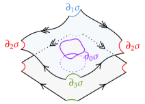
(b)

Figure 17: (a) Surface $B^{\prime}$, and (b) Section $\sigma:B^{\prime}\to M^{\prime}$

Removing small open discs $D_{1}$, $D_{2}$ and $D_{3}$ on $B$ around the three singular points $[c_{1}^{\prime}],[c_{3}^{\prime}],[c_{2}^{\prime}]=[c_{4}^{\prime}]$ and one small disc $D_{0}$ around a regular point $[x_{0}]$ in $B$, with $x_{0}\in\mathring{P}$, we have the surface with boundary $B^{\prime}:=B\setminus\sqcup_{i}D_{i}$. The $3$-manifold $M^{\prime}=\zeta^{-1}(B^{\prime})$ is a principal $\mathbb{S}^{1}$-bundle over $B^{\prime}$. Notice that $M\setminus M^{\prime}$ is made of four solid tori $W_{0},W_{1},W_{2},W_{3}$, where $W_{i}=\zeta^{-1}D_{i}$.

For any section $\sigma:D^{\prime}\to M^{\prime}$, lets denote $\sigma|_{\partial D_{i}}$ by $\partial_{i}\sigma$. Remember the curve $d$ defined in Subsection 26. Shrinking $F^{-1}(d)$ inside the torus $\partial_{\infty}Q^{\prime}$ we can build a section $\sigma:D^{\prime}\to M^{\prime}$ satisfying the identities (See figure 16)

$$\partial_{0}\sigma=\pi(d),\quad\partial_{1}\sigma=-\pi(c_{2}),\quad\partial_{2}\sigma=-\pi(b_{2}),\quad\partial_{3}\sigma=-\pi(a)$$

in $H_{1}(M,\mathbb{Q})$.

The identity $n_{i}\partial_{i}\sigma=-l_{i}\omega_{i}$ in $H_{1}(M,\mathbb{Q})$ holds for $i=1,2,3$, where $\omega_{i}$ is the orbit of a point in $\partial W_{i}$. Furthermore, $\omega_{0}=\omega_{1}=\omega_{2}=\omega_{3}=s$ in $H_{1}(M,\mathbb{Q})$.

Let us prove the identity $n_{i}\partial_{i}\sigma=-l_{i}\omega_{i}$ for $i=1$.

Consider a generator $s^{\prime}$ of the fundamental group of $\pi(\partial C_{1})$.

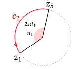
(a)

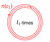
(b)

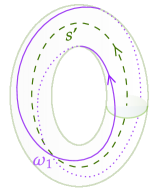
(c)

Figure 18: (a) Curve $c_{2}$ in $\partial C_{1}$, (b) loop $\pi(c_{2})$ in $\pi(\partial C_{1})$, and (c) loop $\omega_{1}$ on the solid torus $W_{1}$.

We can think of $\omega_{1}$ as $\mathbb{S}^{1}\to M$ given by

$$\gamma\mapsto\pi\circ F\left[\frac{(c_{1}^{\prime}+zp_{1}^{\prime})}{\sqrt{1-|z|^{2}}}+\gamma q\right]$$

for a fixed $z$.

Notice $\omega_{1}=n_{1}s^{\prime}$, because $\omega_{1}$ is homotopic to the curve $\gamma\mapsto[c_{1}^{\prime}+\gamma q]$ in $M$, which is a curve that goes $n_{1}$ times around the circle $\pi(\partial C_{1})$, and $\partial_{1}\sigma=-l_{1}s^{\prime}$, because $\partial_{1}\sigma=-\pi(c_{2})$ in $M$ and $\pi(c_{2})$ goes $l_{1}$ times around the circle $\pi(\partial C_{1})$, since in $\partial C_{1}$ the curve $c_{2}$ is constructed as the curve going from $z_{5}$ to $z_{1}$ following the natural orientation of the circle and $I_{1}z_{1}=z_{5}$.

Therefore, we have

$$n_{1}\partial_{1}\sigma=-l_{1}\omega_{1}\quad\text{in}\quad H_{1}(M,\mathbb{Q}).$$

In the case of $i=0$, we have $\partial_{0}\sigma=\pi(d)$ and, therefore, we have $\partial_{0}\sigma=f\omega_{0}$ in $H_{1}(M^{\prime},\mathbb{Z})$, because $d=fs$.

Note $\partial D_{i}$ is oriented in opposite direction of $\partial B^{\prime}$. Therefore, in $H_{1}(M,\mathbb{Q})$ we can write

$$\partial\sigma=\sum_{i=0}^{3}-\partial_{i}\sigma=\left(-f+\frac{l_{1}}{n_{1}}+\frac{l_{2}}{n_{2}}+\frac{l_{3}}{n_{3}}\right)s$$

and, therefore,

$$e(M)=f-\frac{l_{1}}{n_{1}}-\frac{l_{2}}{n_{2}}-\frac{l_{3}}{n_{3}}.$$

7.6.  Holonomy of the quadrangle

In Subsection 26 we define the curve $d$, shown in Figure 16, and the integer $f$, necessary to calculate the Euler number. In order to express this integer explicitly we use the concept of holomony of a transversal triangle of bisectors.

Given a counterclockwise oriented transversal triangle of bisectors $\Delta(L_{1},L_{2},L_{3})$, let $M_{1},M_{2},M_{3}$ be the middle slices (see Subsection 2.3) of the segments of bisectors $\mathrm{B}[L_{1},L_{2}]$, $\mathrm{B}[L_{2},L_{3}]$, $\mathrm{B}[L_{3},L_{1}]$. The product $I$ of the reflections in the middle slices $M_{1}$, $M_{2}$, $M_{3}$ (in that order) is called the holonomy of the triangle $\Delta(L_{1},L_{2},L_{3})$ [AGG, Subsection 2.5.1]. Note that $I$ stabilizes $L_{1}$.

The triangle $\Delta(L_{1},L_{2},L_{3})$ is respectively called elliptic, parabolic, or hyperbolic when the holonomy $I$ restricted to $L_{1}$ is an elliptic, parabolic, or hyperbolic isometry of the Poincaré disc $L_{1}$. The holonomy of a counterclockwise oriented transversal triangle cannot be trivial, that is, $I$ restricted to $L_{1}$ is never the identical isometry; moreover, parabolic triangles are always $L$-parabolic, that is, the holonomy restricted to $L_{1}$ moves its non-fixed points in the clockwise sense [AGG, Theorem 2.24]. In the case of a hyperbolic triangle, the action of $I$ on $L_{1}$ divides $\partial_{\infty}L_{1}$ into the $L$ and $R$-parts: the $L$-part (respectively, the $R$-part) consists of those points that are moved by $I$ in the clockwise sense (respectively, counterclockwise sense). In the elliptic and parabolic cases, all (non-fixed) points belong to the $L$-part.

A simple closed curve in the torus $\partial_{\infty}\Delta(L_{1},L_{2},L_{3})$ is called a trivialing curve of the triangle if it generates the fundamental group of the solid torus $\Delta(L_{1},L_{2},L_{3})$ and is contractible in the ideal boundary of the polyhedron bounded by $\Delta(L_{1},L_{2},L_{3})$ (see Section 6).

As introduced in Subsection 7.4, let

$$d:=m_{1}\cup a\cup m_{2}\cup b_{2}\cup m_{3}\cup m_{4}\cup c_{2}$$ (26)

be the oriented closed curve in the boundary of the solid torus $\partial_{\infty}Q$, where $Q$ stands for the polyhedron of the quadrangle $\mathcal{Q}$. Remind that the group $H_{1}(\partial_{\infty}Q,\mathbb{Z})$ is generated by $[s]$, where $[s]$ stands for the naturally oriented boundary of $C_{1}$. Hence, $[d]=f[s]$ for some $f\in\mathbb{Z}$. In order to express $f$ in terms of the holonomies of the triangles $\Delta(C_{1},C_{2},C_{4})$ and $\Delta(C_{3},C_{4},C_{2})$, we introduce more points and curves:

$\bullet$ the meridional curve $m_{2}^{\prime}\subset\partial_{\infty}\mathrm{B}[C_{2},C_{3}]$ that begins at $z_{2}$ and ends at $z_{3}^{\prime}\in\partial_{\infty}C_{3}$;

$\bullet$ the meridional curve $m\subset\partial_{\infty}\mathrm{B}[C_{2},C_{4}]$ that begins at $z_{2}$ and ends at $z_{4}^{\prime}\in\partial_{\infty}C_{4}$;

$\bullet$ the meridional curve $m_{3}^{\prime}\subset\partial_{\infty}\mathrm{B}[C_{4},C_{3}]$ that begins at $z_{4}^{\prime}$ and ends at $z_{3}^{\prime\prime}\in\partial_{\infty}C_{3}$;

$\bullet$ the naturally oriented arc $b\subset\partial_{\infty}C_{3}$ that begins at $z_{3}^{\prime}$ and ends at $z_{3}^{\prime\prime}$;

$\bullet$ the meridional curve $m_{4}^{\prime}\subset\partial_{\infty}\mathrm{B}[C_{4},C_{1}]$ that begins at $z_{4}^{\prime}$ and ends at $z_{5}^{\prime}\in\partial_{\infty}C_{1}$;

$\bullet$ the naturally oriented arc $c\in\partial_{\infty}C_{1}$ that begins at $z_{5}^{\prime}$ and ends at $z_{1}$.

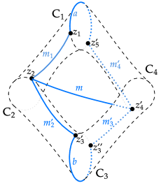
Figure 19: Auxiliary curves

Denote by $I$ the holonomy of the triangle $\Delta(C_{1},C_{2},C_{4})$ and by $J$ the holonomy of the triangle $\Delta(C_{3},C_{4},C_{2})$. By the definition of holonomy of a triangle, we have $z_{3}^{\prime\prime}=J^{-1}z_{3}^{\prime}$ and $z_{5}^{\prime}=Iz_{1}$.

Let us assume that $z_{1}$ belongs to the $L$-part of $\Delta(C_{1},C_{2},C_{4})$ and that $z_{3}^{\prime}$ belongs to the $L$-part of $\Delta(C_{3},C_{4},C_{2})$ (this is harmless because all the triangles that appear in the constructed orbibundles are elliptic). In this case, by [AGG, Theorem 2.24], the closed oriented curve $m_{1}\cup m\cup m_{4}^{\prime}\cup c$ is a trivializing curve of $\Delta(C_{1},C_{2},C_{4})$. Similarly, ${m_{3}^{\prime}}^{-1}\cup m^{-1}\cup m_{2}^{\prime}\cup b$ is a trivializing curve of the triangle $\Delta(C_{3},C_{4},C_{2})$. (We denote by $x^{-1}$ the (not necessarily closed) curve $x$ taken with the opposite orientation.) By [AGG, Remark 2.21], $m_{1}\cup m_{2}^{\prime}\cup b\cup{m_{3}^{\prime}}^{-1}\cup m_{4}^{\prime}\cup c$ is a trivializing curve of the quadrangle $\mathcal{Q}$, that is, it generates the fundamental group of $\mathcal{Q}$ and is contractible in $\partial_{\infty}Q$. In terms of $1$-chains modulo boundaries, this means that

$$[m_{1}]+[m_{2}^{\prime}]+[b]-[m_{3}^{\prime}]+[m_{4}^{\prime}]+[c]=0.$$ (27)

Finally, we introduce the following arcs:

$\bullet$ the naturally oriented simple arc $b_{1}\subset\partial_{\infty}C_{3}$ that begins at $z_{3}^{\prime}$ and ends at $z_{3}$;

$\bullet$ the naturally oriented simple arc $b_{3}\subset\partial_{\infty}C_{3}$ that begins at $I_{3}z_{3}$ and ends at $z_{3}^{\prime\prime}$;

$\bullet$ the naturally oriented simple arc $c_{1}\subset\partial_{\infty}C_{1}$ that begins at $z_{5}$ and ends at $z_{5}^{\prime}$.

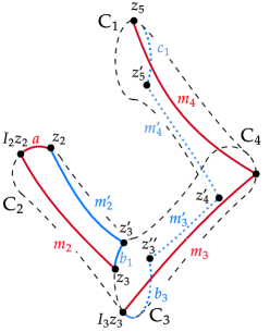
Figure 20: Cylinders $\partial_{\infty}\mathrm{B}[C_{2},C_{3}]$ and $\partial_{\infty}\mathrm{B}[C_{3},C_{4}]\cup\partial_{\infty}\mathrm{B}[C_{4},C_{1}]$.

By looking at the cylinder $\partial_{\infty}\mathrm{B}[C_{2},C_{3}]$, it is easy to see that

$$[a]+[m_{2}]-[b_{1}]-[m_{2}^{\prime}]=0.$$ (28)

Similarly, by considering the cylinder $\partial_{\infty}\mathrm{B}[C_{3},C_{4}]\cup\partial_{\infty}\mathrm{B}[C_{4},C_{1}]$, one obtains that

$$[m_{3}]+[m_{4}]+[c_{1}]-[m_{4}^{\prime}]+[m_{3}^{\prime}]-[b_{3}]=0.$$ (29)

It follows from equations (26), (28), and (29) that

$$[d]=[m_{1}]+[a]+[m_{2}]+[b_{2}]+[m_{3}]+[m_{4}]+[c_{2}]=\\ [m_{1}]+[m_{2}^{\prime}]+[b_{1}]+[b_{2}]+[b_{3}]-[m_{3}^{\prime}]+[m_{4}^{\prime}]-[c_{1}]+[c_{2}].$$ (30)

We introduce the following notation. Let $C$ be an oriented circle and let $t_{1},t_{2},t_{3}\in C$. We define $o(t_{1},t_{2},t_{3})=1$ if $t_{1},t_{2},t_{3}$ are pairwise distinct and not in cyclic order. Otherwise, we put $o(t_{1},t_{2},t_{3})=0$.

Lemma 31.

Let $C$ be an oriented circle and let $t_{1},t_{2},t_{3},t_{4}\in C$ be such that $t_{3}\neq t_{1}\neq t_{4}$. Following the orientation of $C$, we define four simple arcs (some of them may consist of a single point): $a_{i}\subset C$ joining $t_{i}$ and $t_{i+1}$ for $i=1,2,3$ and $a\subset C$ joining $t_{1}$ and $t_{4}$. Then we have

$$[a_{1}]+[a_{2}]+[a_{3}]-[a]=o(t_{1},t_{2},t_{3})[C]+o(t_{3},t_{4},t_{1})[C]$$

in $C_{1}(C,\mathbb{Z})/\partial C_{0}(C,\mathbb{Z})$. (Of course, we take $[C]$ as a generator of $H_{1}(C,\mathbb{Z})$.)

Proof. Define the following oriented simple arcs: $a_{4}$ joining $t_{4}$ and $t_{1}$; $m_{1}$ joining $t_{1}$ and $t_{3}$; and $m_{2}$ joining $t_{3}$ and $t_{1}$. It follows from $t_{1}\neq t_{4}$ that $[a]+[a_{4}]=[C]$. Analogously, $t_{1}\neq t_{3}$ implies $[m_{1}]+[m_{2}]=[C]$. By drawing the corresponding arcs in $C$, it is easy to see that $[a_{1}]+[a_{2}]-[m_{1}]=o(t_{1},t_{2},t_{3})[C]$ and $[a_{3}]+[a_{4}]-[m_{2}]=o(t_{3},t_{4},t_{1})[C]$. So,

$$[a_{1}]+[a_{2}]+[a_{3}]-[a]=[a_{1}]+[a_{2}]+[a_{3}]+[a_{4}]-[C]=$$

$$=o(t_{1},t_{2},t_{3})[C]+[m_{1}]+o(t_{3},t_{4},t_{1})[C]+[m_{2}]-[C]=o(t_{1},t_{2},t_{3})[C]+o(t_{3},t_{4},t_{1})[C].$$ _■

Applying Lemma 31 to the naturally oriented circle $\partial_{\infty}C_{3}$ and the points $z_{3}^{\prime},z_{3},I_{3}z_{3},J^{-1}z_{3}^{\prime}\in\partial_{\infty}C_{3}$ (note that $z_{3}^{\prime}\neq J^{-1}z_{3}^{\prime}$ always hold and one can assume that $z_{3}^{\prime}\neq I_{3}z_{3}$) we obtain

$$[b_{1}]+[b_{2}]+[b_{3}]=[b]+o(z_{3}^{\prime},z_{3},I_{3}z_{3})[s]+o(I_{3}z_{3},J^{-1}z_{3}^{\prime},z_{3}^{\prime})[s].$$ (32)

In the naturally oriented circle $\partial_{\infty}C_{1}$ we have

$$[c_{1}]+[c]=[c_{2}]+o(I_{1}^{-1}z_{1},Iz_{1},z_{1})[s]$$ (33)

since $[\partial_{\infty}C_{1}]=[s]$. Therefore, it follows from (30), (32), and (33) that

$$[d]=[m_{1}]+[m_{2}^{\prime}]+[b]-[m_{3}^{\prime}]+[m_{4}^{\prime}]+[c]+o(z_{3}^{\prime},z_{3},I_{3}z_{3})[s]+o(I_{3}z_{3},J^{-1}z_{3}^{\prime},z_{3}^{\prime})[s]-o(I_{1}^{-1}z_{1},Iz_{1},z_{1})[s].$$

Hence, by (27),

$$[d]=o(z_{3}^{\prime},z_{3},I_{3}z_{3})[s]+o(I_{3}z_{3},J^{-1}z_{3}^{\prime},z_{3}^{\prime})[s]-o(I_{1}^{-1}z_{1},Iz_{1},z_{1})[s],$$

that is,

$$f=o(z_{3}^{\prime},z_{3},I_{3}z_{3})+o(z_{3}^{\prime},I_{3}z_{3},J^{-1}z_{3}^{\prime})-o(z_{1},I_{1}^{-1}z_{1},Iz_{1}).$$

8 Toledo invariant

Let $\rho:G\to\mathrm{\mathrm{PU}}(2,1)$ be a faithful $\mathrm{\mathrm{PU}}(2,1)$-representation of the turnover group $G$ and let $\phi:\mathbb{H}_{\mathbb{R}}^{2}\to\mathbb{H}_{\mathbb{C}}^{2}$ be a $G$-equivariant map. The Toledo invariant of $\rho$ is defined by the formula

$$\tau(\rho)=4\cdot\frac{1}{2\pi}\int_{P}\phi^{\ast}\omega,$$

where $P$ is a fundamental domain in $\mathbb{H}_{\mathbb{R}}^{2}$ for the action of $G$ (see subsection 3.1 and figure 4). The number $\tau$ does not depend on the choice of the $G$-equivariant map $\phi$. For details about the Toledo invariant in the context of orbifolds, see [Bot1, Definition 35] and [Krebs]). The factor $4$ in our formula for the Toledo invariant comes from the fact that our metric is four times the usual one.

Let $\mathcal{Q}$ be the quadrangle associated to the representation $\rho$. We assume that it satisfies the quadrangle conditions in subsection 6.2. In order to calculate the Toledo invariant of $\rho$, we introduce in $\mathcal{Q}$ several curves as illustrated in figure 21. First, we define the oriented meridional curves

$$m_{1}:=[c_{1}^{\prime},c_{2}]\subset\mathrm{B}[C_{1},C_{2}],\quad m_{2}:=[c_{2},c_{3}^{\prime}]\subset\mathrm{B}[C_{2},C_{3}],\quad m_{3}^{-1}:=I_{3}m_{2}=[c_{4},I_{3}c_{3}^{\prime}]\subset\mathrm{B}[C_{3},C_{4}],$$

$$m_{4}^{-1}:=I_{1}^{-1}m_{1}=[I_{1}^{-1}c_{1}^{\prime},c_{4}]\subset\mathrm{B}[C_{4},C_{1}],$$

with $c_{1}^{\prime}\in C_{1}$ and $c_{3}^{\prime}\in C_{3}$ (note that $c_{4}=I_{1}^{-1}c_{2}=I_{3}c_{2}$). We also introduce the oriented geodesics

$$h_{1}:=\mathrm{\mathrm{G}}[c_{1},c_{1}^{\prime}]\subset C_{1},\quad h_{2}:=\mathrm{\mathrm{G}}[c_{3}^{\prime},c_{3}]\subset C_{3},\quad h_{3}^{-1}:=I_{3}h_{2}=\mathrm{\mathrm{G}}[I_{3}c_{3}^{\prime},c_{3}]\subset C_{3},$$

$$h_{4}^{-1}:=I_{1}^{-1}h_{1}=\mathrm{\mathrm{G}}[c_{1},I_{1}^{-1}c_{1}^{\prime}]\subset C_{1}$$

Figure 21: Curve $c$.

thus obtaining the closed oriented curve

$$\zeta:=h_{1}\cup m_{1}\cup m_{2}\cup h_{2}\cup h_{3}\cup m_{3}\cup m_{4}\cup h_{4}.$$ (34)

Following the notation in Subsection 7.1, let $\alpha_{1},\beta_{1},\gamma_{1}^{-1}$ be the eigenvalues of $I_{1},I_{2},I_{3}$ corresponding to negative eigenvectors. The proof below is similar to that of [AGG, Proposition 2.7]. The strategy of the proof is the following. By Stokes theorem, the Toledo invariant of $\rho$ can be obtained by integrating a Kähler potential along $\zeta$ because the quadrangle conditions allow one to build a $G$-equivariant map $\mathbb{H}_{\mathbb{R}}^{2}\to\mathbb{H}_{\mathbb{C}}^{2}$ sending $\partial P$ to $\zeta$ (note that $\zeta$ is the boundary of a smooth disc inside the real $4$-ball $Q$). A potential for the Kähler is obtained by choosing a basepoint $c\in\mathbb{H}_{\mathbb{C}}^{2}$ as in formula (2). The boundary of $\zeta$ is made of meridional curves and geodesics. Since each of these curves is contained in a real plane, it follows from formula (2) that the integral of a Kähler potential along the curve vanishes when we choose the basepoint $c$ in the curve (say, we can take $c$ as the starting point of the curve). So, the contributions to the Toledo invariant come from the changes of basepoints which are explicitly given in (3).

Proposition 35.

Let $\rho:G\to\mathrm{\mathrm{PU}}(2,1)$, $g_{j}\mapsto I_{j}$, be a representation satisfying the quadrangle conditions 6.2. Then $\tau\equiv\displaystyle\frac{\mathrm{\mathrm{Arg}}(\alpha_{1}\beta_{1}\gamma_{1}^{-1})}{\pi}\mod 2$, where $\tau$ stands for the Toledo invariant of $\rho$.

Proof. Note that $\alpha_{1}\beta_{1}\gamma_{1}^{-1}$ is well-defined for $\rho$ because we assume the equality $I_{3}I_{2}I_{1}=1$ in $\mathrm{\mathrm{SU}}(2,1)$. We take the quadrangle of bisectors $\mathcal{Q}$ of $\rho$ described in Subsection 6.2, the closed oriented curve $\zeta\subset\mathcal{Q}$ defined in (34), and the geodesic polygon $P\subset\mathbb{H}_{\mathbb{R}}^{2}$ defined in subsection 3.1. Let $D\subset\mathbb{H}_{\mathbb{C}}^{2}$ be a disc with $\partial D=\zeta$ and let $\varphi:\mathbb{H}_{\mathbb{R}}^{2}\to\mathbb{H}_{\mathbb{C}}^{2}$ be a $\rho$-equivariant map such that $\varphi P=D$, $\varphi v_{j}=c_{j}$, and

$$\varphi e_{1}=h_{1}\cup m_{1},\quad\varphi e_{2}=m_{2}\cup h_{2},\quad\varphi e_{3}=h_{3}\cup m_{3},\quad\varphi e_{4}=m_{4}\cup h_{4}$$

(see Figure 4). Then $\tau=\frac{4}{2\pi}\int_{P}\varphi^{*}\omega$, that is,

$$\tau=\frac{2}{\pi}\int_{D}\omega=\frac{2}{\pi}\int_{\partial D}P_{c_{2}}=\frac{2}{\pi}\sum_{j=1}^{4}\left(\int_{m_{j}}P_{c_{2}}+\int_{h_{j}}P_{c_{2}}\right),$$

where $P_{c_{2}}$ is a Kähler primitive with basepoint $c_{2}\in\mathbb{H}_{\mathbb{C}}^{2}$. The choice of the basepoint implies $\int_{m_{1}}P_{c_{2}}=\int_{m_{2}}P_{c_{2}}=0$. The remaining integrals can be evaluated with the aid of the formula relating primitives based on distinct points:

$$J_{1}:=\int_{h_{2}}P_{c_{2}}=\int_{h_{2}}(P_{c_{2}}-P_{c_{3}^{\prime}})=\int_{h_{2}}\mathrm{d}f_{c_{2},c_{3}^{\prime}}=$$

$$=\frac{1}{2}\mathrm{\mathrm{Arg}}\left(\frac{\langle c_{2},c_{3}\rangle\langle c_{3},c_{3}^{\prime}\rangle}{\langle c_{2},c_{3}^{\prime}\rangle}\right)-\frac{1}{2}\mathrm{\mathrm{Arg}}\left(\frac{\langle c_{2},c_{3}^{\prime}\rangle\langle c_{3}^{\prime},c_{3}^{\prime}\rangle}{\langle c_{2},c_{3}^{\prime}\rangle}\right)=\frac{1}{2}\mathrm{\mathrm{Arg}}\left(\frac{\langle c_{2},c_{3}\rangle\langle c_{3},c_{3}^{\prime}\rangle}{\langle c_{2},c_{3}^{\prime}\rangle}\right)-\frac{\pi}{2};$$

$$J_{2}:=\int_{h_{3}}P_{c_{2}}=\int_{h_{3}}(P_{c_{2}}-P_{c_{3}})=\int_{h_{3}}\mathrm{d}f_{c_{2},c_{3}}=\frac{1}{2}\mathrm{\mathrm{Arg}}\frac{\langle c_{2},I_{3}c_{3}^{\prime}\rangle\langle I_{3}c_{3}^{\prime},c_{3}\rangle}{\langle c_{2},c_{3}\rangle}-\frac{1}{2}\mathrm{\mathrm{Arg}}\frac{\langle c_{2},c_{3}\rangle\langle c_{3},c_{3}\rangle}{\langle c_{2},c_{3}\rangle}=$$

$$=\frac{1}{2}\mathrm{\mathrm{Arg}}\left(\frac{\langle c_{2},I_{3}c_{3}^{\prime}\rangle\langle I_{3}c_{3}^{\prime},c_{3}\rangle}{\langle c_{2},c_{3}\rangle}\right)-\frac{\pi}{2}=\frac{1}{2}\mathrm{\mathrm{Arg}}\left(\gamma_{1}^{-1}\frac{\langle c_{2},I_{3}c_{3}^{\prime}\rangle\langle c_{3}^{\prime},c_{3}\rangle}{\langle c_{2},c_{3}\rangle}\right)-\frac{\pi}{2}.$$

Similarly, one obtains

$$J_{3}:=\int_{m_{3}}P_{c_{2}}=\frac{1}{2}\mathrm{\mathrm{Arg}}\left(\beta_{1}\frac{\langle c_{2},I_{1}^{-1}c_{2}\rangle\langle c_{2},c_{3}^{\prime}\rangle}{\langle c_{2},I_{3}c_{3}^{\prime}\rangle}\right)-\frac{\pi}{2};\quad J_{4}:=\int_{m_{4}}P_{c_{2}}=\frac{1}{2}\mathrm{\mathrm{Arg}}\left(\frac{\langle c_{2},I_{1}^{-1}c_{1}^{\prime}\rangle\langle c_{1}^{\prime},c_{2}\rangle}{\langle c_{2},I_{1}^{-1}c_{2}\rangle}\right)-\frac{\pi}{2};$$

$$J_{5}:=\int_{h_{4}}P_{c_{2}}=\frac{1}{2}\mathrm{\mathrm{Arg}}\left(\alpha_{1}\frac{\langle c_{2},c_{1}\rangle\langle c_{1},c_{1}^{\prime}\rangle}{\langle c_{2},I_{1}^{-1}c_{1}^{\prime}\rangle}\right)-\frac{\pi}{2};\quad J_{6}:=\int_{h_{1}}P_{c_{2}}=\frac{1}{2}\mathrm{\mathrm{Arg}}\left(\frac{\langle c_{2},c_{1}^{\prime}\rangle\langle c_{1}^{\prime},c_{1}\rangle}{\langle c_{2},c_{1}\rangle}\right)-\frac{\pi}{2}.$$

We have $\tau=\displaystyle\frac{2}{\pi}\sum_{j}J_{j}$. Calculating mod $2$, we multiply the arguments of every $\mathrm{\mathrm{Arg}}$ function participating in the previous sum thus obtaining the result. _■

The Toledo invariant is in fact an invariant of the faithful representation $\rho:G\to\mathrm{\mathrm{PU}}(2,1)$; it does not depend on the quadrangle conditions. However, we only consider here representations satisfying such condition since discreteness is our main concern (see Section 6).

9 Explicit example with trivial Euler number.

We work with the standard model for the complex hyperbolic plane: consider the Hermitian form

$$\langle z,w\rangle=-z_{1}\overline{w_{1}}+z_{2}\overline{w_{2}}+z_{3}\overline{w_{3}}$$

on $\mathbb{C}^{3}$ and the complex hyperbolic plane $\mathbb{H}_{\mathbb{C}}^{2}$, formed by points $[z_{1},z_{2},z_{3}]$ of the complex projective plane $\mathbb{P}_{\mathbb{C}}^{2}$ satisfying $-|z_{1}|^{2}+|z_{2}|^{2}+|z_{3}|^{2}<0$.

The parameters we set are

$$n_{1}=n_{2}=n_{3}=5,\quad k_{1}=k_{3}=0,\quad k_{2}=2,\quad d=1,\quad s=2.4,\quad t=0.9,$$

taken from the Table 1. They correspond to an example of a non-rigid representation whose associated disc orbibundle has trivial Euler number, as we will show.

The eigenvalues, as set in the beginning of Section 4, are

$$\alpha_{1}=\exp\left(\frac{2(n_{1}-k_{1})\pi i}{3n_{1}}\right),\quad \alpha_{2}=\exp\left(\frac{2(n_{1}-k_{1}-3)\pi i}{3n_{1}}\right),\quad \alpha_{3}=\exp\left(\frac{2(2k_{1}+n_{1}+3)\pi i}{3n_{1}}\right),$$

$$\beta_{1}=\exp\left(\frac{-2k_{2}\pi i}{3n_{2}}\right),\quad \beta_{2}=\exp\left(\frac{2(-k_{2}-3)\pi i}{3n_{2}}\right),\quad \beta_{3}=\exp\left(\frac{2(2k_{2}+3)\pi i)}{3n_{2}}\right),$$

$$\gamma_{1}^{-1}=\exp\left(\frac{2(2n_{3}d-k_{3})\pi i}{3n_{3}}\right),\quad \gamma_{2}^{-1}=\exp\left(\frac{2(2n_{3}d-k_{3}-3)\pi i}{3n_{3}}\right),\quad \gamma_{3}^{-1}=\exp\left(\frac{2(2n_{3}d+2k_{3}+3)\pi i)}{3n_{3}}\right).$$

Define the following terms, which we use to compute $I_{2}$,

$$\alpha_{ij}:=\alpha_{i}-\alpha_{j},\quad\beta_{ij}:=\beta_{i}-\beta_{j},\quad\gamma_{ij}:=\gamma_{i}-\gamma_{j},$$

$$k:=\frac{1}{\beta_{23}}\left(\gamma_{1}+\gamma_{2}+\gamma_{3}-\alpha_{1}(\beta_{1}+\beta_{2}-\beta_{3})-\beta_{3}(\alpha_{2}+\alpha_{3})\right),$$

$$z:=\displaystyle\frac{\beta_{13}}{\beta_{23}}\big{(}\alpha_{21}s+\alpha_{31}t\big{)}+k,$$

$$M:=\left[\begin{smallmatrix}\alpha_{21}&\alpha_{31}\\ \mathrm{\mathrm{Im}}\alpha_{21}&\mathrm{\mathrm{Im}}\alpha_{31}\end{smallmatrix}\right].$$

Following the Section 5, the matrices $I_{1},I_{2}$ are computed by the formulas

$$I_{1}=\left[\begin{smallmatrix}\alpha_{1}&0&0\\ 0&\alpha_{2}&0\\ 0&0&\alpha_{3}\end{smallmatrix}\right],\qquad I_{2}=\left[\begin{smallmatrix}-v_{1}^{2}\beta_{23}+u_{1}^{2}\beta_{13}+\beta_{3}&v_{1}\overline{v}_{2}\beta_{23}-u_{2}u_{1}\beta_{13}&v_{1}\overline{v}_{3}\beta_{23}-u_{3}u_{1}\beta_{13}\\ -v_{1}v_{2}\beta_{23}+u_{1}u_{2}\beta_{13}&|v_{2}|^{2}\beta_{23}-u_{2}^{2}\beta_{13}+\beta_{3}&v_{2}\overline{v}_{3}\beta_{23}-u_{3}u_{2}\beta_{13}\\ -v_{1}v_{3}\beta_{23}+u_{1}u_{3}\beta_{13}&\overline{v}_{2}v_{3}\beta_{23}-u_{2}u_{3}\beta_{13}&|v_{3}|^{2}\beta_{23}-u_{3}^{2}\beta_{13}+\beta_{3}\end{smallmatrix}\right],$$ (36)

where we define

$$u_{1}:=\sqrt{1+s+t},\quad u_{2}:=\sqrt{s},\quad u_{3}:=\sqrt{t},$$

and $v_{1},v_{2},v_{3}$ is given by

$$v_{2}=\frac{1}{2v_{1}\sqrt{s(1+s+t)}}\big{(}-t|v_{3}|^{2}+(1+s+t)v_{1}^{2}+s|v_{2}|^{2}+i\sqrt{\Delta}\big{)},$$

$$v_{3}=\frac{1}{2v_{1}\sqrt{t(1+s+t)}}\big{(}-s|v_{2}|^{2}+(1+s+t)v_{1}^{2}+t|v_{3}|^{2}-i\sqrt{\Delta}\big{)}.$$

In the above formula we use

$$\Delta:=4v_{1}^{2}|v_{2}|^{2}s(1+s+t)-\big{(}-t|v_{3}|^{2}+(1+s+t)v_{1}^{2}+s|v_{2}|^{2}\big{)}^{2},$$

$$|v_{2}|^{2}:=\mathrm{\mathrm{Im}}(\alpha_{31}\overline{z})/\det M,$$

$$|v_{3}|^{2}:=-\mathrm{\mathrm{Im}}(\alpha_{21}\overline{z})/\det M,$$

$$v_{1}:=\sqrt{1+|v_{2}|^{2}+|v_{3}|^{2}}.$$

Note that in order to compute $v_{2},v_{3}$ we must have the formulas defining $\Delta$, $|v_{2}|^{2}$, and $|v_{3}|^{2}$ non-negative. Once we have $I_{1},I_{2}$, we define $I_{3}:=I_{1}^{-1}I_{2}^{-1}$.

Using the described framework, we obtain the matrices

$$I_{1}=\left[\begin{smallmatrix}-0.5+0.8660254038i&\quad\,\,0&\quad\,\,0\\ 0&\quad\,\,0.6691306064+0.7431448255i&\quad\,\,0\\ 0&\quad\,\,0&\quad\,\,-0.9781476007-0.2079116908i\\ \end{smallmatrix}\right],$$

$$I_{2}=\left[\begin{smallmatrix}4.806086358-0.9638895607i&\,\,-4.070625549-0.2082686381i&\,\,-2.395307321+0.8226079388i\\ 3.683729972+0.0360116289i&\,\,-3.385353305-0.9825139687i&\,\,-1.430999775+0.3121734931i\\ 3.027105153-0.5413134207i&\,\,-2.276681096-0.06434808952i&\,\,-2.229750048+0.545144991i\\ \end{smallmatrix}\right],$$

$$I_{3}=\left[\begin{smallmatrix}-1.568290333-4.644137659i&\,\,1.873051971+3.172197922i&\,\,1.044761403+2.892206673i\\ 2.569006381-3.164423233i&\,\,-1.535093338+3.173237958i&\,\,-1.475577052+1.734961052i\\ -2.513993916-0.3066195865i&\,\,1.464633515+0.007830170545i&\,\,2.294366676+0.06964116243i\\ \end{smallmatrix}\right].$$

They satisfy $I_{3}I_{2}I_{1}=1,\,I_{1}^{5}=e^{-2\pi i/3},\,I_{2}^{5}=e^{2\pi i/3},\,I_{3}^{5}=e^{2\pi i/3}$ in $\mathrm{\mathrm{SU}}(2,1)$.

The positive eigenvectors $p_{1},p_{2},p_{3}$ for $I_{1},I_{2},I_{3}$ with respect to $\alpha_{2},\beta_{2},\gamma_{2}$ are

$$p_{1}=\left[\begin{smallmatrix}0\\ 1\\ 0\end{smallmatrix}\right],\quad p_{2}=\left[\begin{smallmatrix}1.648291445\\ 1.794969768+0.1092825754i\\ 0.6716832499-0.1784576984i\\ \end{smallmatrix}\right],\quad p_{3}=\left[\begin{smallmatrix}1.662566196+0.7047909878i\\ 1.026420435+1.623659667i\\ 0.7556765638\\ \end{smallmatrix}\right],$$

and

$$p_{4}:=I_{1}^{-1}p_{2}=\left[\begin{smallmatrix}-0.8241457224-1.427462264i\\ 1.28228199-1.260798179i\\ -0.6199019175+0.3142087697i\\ \end{smallmatrix}\right].$$

Condition (Q1) ensuring that the complex geodesics $C_{i}=\mathbb{P}(p^{\perp})\cap\mathbb{H}_{\mathbb{C}}^{2}$ are pairwise ultraparallel is satisfied:

$$\mathrm{\mathrm{ta}}(p_{1},p_{2})\simeq 3.234,\quad\mathrm{\mathrm{ta}}(p_{2},p_{4})\simeq 9.304,\quad\mathrm{\mathrm{ta}}(p_{2},p_{3})\simeq 3.197.$$

Thus, we can connect the complex geodesics with segments of bisectors to construct the quadrangle of bisectors

$$\mathcal{Q}=B[C_{1},C_{2}]\cup B[C_{2},C_{3}]\cup B[C_{3},C_{4}]\cup B[C_{4},C_{1}],$$

which will bound our fundamental domain.

Following the notation in (Q2) we have that the transversality and orientation conditions are met

$$1+2t^{2}s\epsilon_{0}-(\epsilon_{0}^{2}t^{2}+s^{2}+t^{2})\simeq 0.0251,\quad 1+2t^{2}s\epsilon_{0}-(\epsilon_{0}^{2}s^{2}+2t^{2})\simeq 3.476,\quad\epsilon_{1}\simeq-0.754,$$

$$1+2t^{\prime 2}s\epsilon_{0}^{\prime}-(\epsilon_{0}^{\prime 2}t^{\prime 2}+s^{2}+t^{\prime 2})\simeq 0.303,\quad 1+2t^{\prime 2}s\epsilon_{0}^{\prime}-(\epsilon_{0}^{\prime 2}s^{2}+2t^{\prime 2})\simeq 3.575,\quad\epsilon_{1}^{\prime}\simeq-0.732$$

where

$$t=\mathrm{\mathrm{ta}}(p_{1},p_{2}),\quad t^{\prime}=\mathrm{\mathrm{ta}}(p_{3},p_{2}),\quad s=\mathrm{\mathrm{ta}}(p_{2},p_{4}),$$

$$\epsilon_{0}+\epsilon_{1}=\frac{\langle p_{1},p_{2}\rangle\langle p_{2},p_{4}\rangle\langle p_{4},p_{1}\rangle}{|\langle p_{1},p_{2}\rangle\langle p_{2},p_{4}\rangle\langle p_{4},p_{1}\rangle|},\quad\epsilon_{0}^{\prime}+\epsilon_{1}^{\prime}=\frac{\langle p_{3},p_{4}\rangle\langle p_{4},p_{2}\rangle\langle p_{2},p_{3}\rangle}{|\langle p_{3},p_{4}\rangle\langle p_{4},p_{2}\rangle\langle p_{2},p_{3}\rangle|}.$$

The first three equations of the six considered above mean that the triangle of bisectors $\Delta(C_{1},C_{2},C_{4})$ is transversal and counterclockwise-oriented. The last three ones guarantee that the triangle of bisectors $\Delta(C_{3},C_{4},C_{2})$ is transversal and counterclockwise-oriented.

Now we must ensure that these two triangles are coupled suitably. More precisely, the conditions below ensure they are transversely adjacent.

The conditions (Q3.1), (Q3.2), (Q3.3) are satisfied via direct computation.

$$\left|\left(\frac{\langle p_{3},p_{1}\rangle\langle p_{2},p_{2}\rangle}{\langle p_{3},p_{2}\rangle\langle p_{2},p_{1}\rangle}\right)-1\right|-\sqrt{1-\frac{1}{\mathrm{\mathrm{ta}}(p_{2},p_{3})}}\sqrt{1-\frac{1}{\mathrm{\mathrm{ta}}(p_{2},p_{1})}}\simeq-0.129,$$

$$\left|\left(\frac{\langle p_{1},p_{3}\rangle\langle p_{4},p_{4}\rangle}{\langle p_{1},p_{4}\rangle\langle p_{4},p_{3}\rangle}\right)-1\right|-\sqrt{1-\frac{1}{\mathrm{\mathrm{ta}}(p_{4},p_{1})}}\sqrt{1-\frac{1}{\mathrm{\mathrm{ta}}(p_{4},p_{3})}}\simeq-0.045,$$

$$\mathrm{\mathrm{Im}}\left(\frac{\langle p_{1},c_{3}\rangle\langle c_{3},p_{2}\rangle}{\langle p_{1},p_{2}\rangle}\right)\simeq 0.713,$$

$$\mathrm{\mathrm{Im}}\left(\frac{\langle p_{4},c_{3}\rangle\langle c_{3},p_{1}\rangle}{\langle p_{4},p_{1}\rangle}\right)\simeq 0.740.$$

The first of the four equations above ensures that $B[C_{1},C_{2}]$ and $B[C_{2},C_{3}]$ are transversal. The second equation does the same for $B[C_{1},C_{4}]$ and $B[C_{4},C_{3}]$. The last two equations guarantees that $c_{3}$, the negative eigenvector of $I_{3}$ corresponding to the eigenvalue $\gamma_{1}^{-1}$, is inside the sector $C_{1}$ defined by the triangle $\Delta(C_{1},C_{2},C_{4})$. The explicit entries for $c_{3}$ are in Equation 38.

The above conditions imply that the quadrangle $\mathcal{Q}$ bounds a fundamental domain candidate for the action of $G(n_{1},n_{2},n_{3})$.

The condition (Q4) is satisfied by our choice of eigenvalues:

$$\frac{\alpha_{2}}{\alpha_{1}}=\exp\left(\frac{-2\pi i}{n_{1}}\right),\quad\frac{\beta_{2}}{\beta_{1}}=\exp\left(\frac{-2\pi i}{n_{2}}\right),\quad\frac{\gamma_{2}^{-1}}{\gamma_{1}^{-1}}=\exp\left(\frac{-2\pi i}{n_{3}}\right).$$

This condition guarantees the tessellation around each vertex $C_{i}$ under the action of the group $G(n_{1},n_{2},n_{3})$. From the Theorem 20 we have a tessellation and, as a consequence, a complex hyperbolic orbifold. The structure of disc orbibundle is induced from the natural foliation by complex geodesics on the quadrangle, as it is discussed in Section 7.

Since all discreetness conditions are met, we have a disc orbibundle over $\mathbb{S}^{2}(5,5,5)$.

Now we compute its Euler number via the formula outlined at the end of the Subsection 7.5 and to do so, we must compute the parameter $f$ following the steps in the Subsection 7.6.

The triangle of bisector $\Delta(C_{1},C_{2},C_{4})$ have holonomy $I$ with trace $|\mathrm{\mathrm{tr}}(I)|=1.9244$ and the triangle of bisector $\Delta(C_{3},C_{4},C_{2})$ have holonomy $J$ with trace $|\mathrm{\mathrm{tr}}(J)|=1.9159$. Therefore, both holonomies are elliptic. Since both triangles are counterclockwise oriented, they are L-elliptic, meaning that the holonomies rotate clockwise, and, as consequence, we can use any $z_{1}$ in our computation of the Euler number. The computation of these holonomies can be done using the formulas outlined in [AGG, Lemma A.33]:

$$|\mathrm{\mathrm{tr}}(I)|=\sqrt{2(1+\epsilon_{0})}\left(1-\frac{1+2t_{12}t_{24}t_{41}\epsilon_{0}-t_{12}^{2}-t_{24}^{2}-t_{41}^{2}}{(t_{12}+1)(t_{24}+1)(t_{41}+1)}\right),$$

$$|\mathrm{\mathrm{tr}}(J)|=\sqrt{2(1+\epsilon_{0}^{\prime})}\left(1-\frac{1+2t_{34}t_{42}t_{23}\epsilon_{0}^{\prime}-t_{34}^{2}-t_{42}^{2}-t_{23}^{2}}{(t_{34}+1)(t_{42}+1)(t_{23}+1)}\right),$$

where $t_{jk}=\sqrt{\mathrm{\mathrm{ta}}(p_{j},p_{k})}$.

We choose $z_{1}=\left[\begin{matrix}1&0&1\end{matrix}\right]^{\textrm{T}}$. To construct the points $z_{2},z_{3},z_{3}^{\prime},z_{3}^{\prime\prime},z_{4}^{\prime},z_{5}^{\prime}$ described in the Subsection 7.6, we need to compute reflections in the middle slice of each bisector segment defining the quadrangle. Middle slice for $B[C_{1},C_{2}],B[C_{2},C_{3}],B[C_{3},C_{4}],B[C_{4},C_{1}]$ have polar points $\mathfrak{m}_{1},\mathfrak{m}_{2},\mathfrak{m}_{3},\mathfrak{m}_{4}$ given by

$$\mathfrak{m}_{i}=\frac{1}{\sqrt{2+2\langle p_{i},p_{i+1}\rangle}}\left(p_{i}+\frac{\langle p_{i},p_{i+1}\rangle}{|\langle p_{i},p_{i+1}\rangle|}p_{i+1}\right),$$

where we assume that $\langle p_{i},p_{i}\rangle=1$. We have

$$\mathfrak{m}_{1}=\left[\begin{smallmatrix}0.6967426286\\ 1.180669147+0.07188230542i\\ 0.2839245175-0.07543513392i\end{smallmatrix}\right],\quad \mathfrak{m}_{2}=\left[\begin{smallmatrix}0.6209147951+0.9915030695i\\ 0.2981752232+1.436781411i\\ 0.3611646254+0.2914178221i\end{smallmatrix}\right],$$

$$\mathfrak{m}_{3}=\left[\begin{smallmatrix}0.3390781806-0.9381337155i\\ 1.346757824-0.4086352516i\\ -0.05189725816-0.1078709913i\end{smallmatrix}\right],\quad \mathfrak{m}_{4}=\left[\begin{smallmatrix}0.1746385463-0.6745010517i\\ 1.182855316\\ -0.2799659635-0.08900927095i\end{smallmatrix}\right].$$

We define $\mathfrak{m}_{5}$ to be the polar for the middle slice of the bisector $B[C_{2},C_{4}]$:

$$\mathfrak{m}_{5}=\frac{1}{\sqrt{2+2\langle p_{2},p_{4}\rangle}}\left(p_{2}+\frac{\langle p_{2},p_{4}\rangle}{|\langle p_{2},p_{4}\rangle|}p_{4}\right).$$

$$\mathfrak{m}_{5}=\left[\begin{smallmatrix}0.2813718628-0.4967217499i\\ 1.073868075-0.4119239074i\\ 0.02003505593+0.05125691089i\end{smallmatrix}\right].$$

The reflection $R_{i}$ on the middle slice $\textbf{middle}_{i}$ is given by

$$x\mapsto-x+2\langle x,\mathfrak{m}_{i}\rangle\mathfrak{m}_{i}$$

The points $z_{2},z_{3},z_{3}^{\prime},z_{3}^{\prime\prime},z_{4}^{\prime},z_{5}^{\prime}$, as described in Subsection 7.6 (see Figures 16 and 19), are given by

$$z_{2}=R_{1}z_{1},\quad z_{3}=R_{2}I_{2}z_{2},\quad z_{3}^{\prime}=R_{2}z_{2},\quad z_{4}^{\prime}=R_{5}z_{2},\quad z_{3}^{\prime\prime}=R_{3}z_{4}^{\prime},\quad z_{5}^{\prime}=R_{4}z_{4}^{\prime}.$$

$$z_{2}=\left[\begin{smallmatrix}-1.575255952+0.105117747i\\ -0.9856481166+0.1187792353i\\ -1.223037447+0.105117747i\end{smallmatrix}\right],\quad z_{3}=\left[\begin{smallmatrix}0.7841986264+0.2491608075i\\ 0.5437649113+0.5867020173i\\ -0.04148256194+0.1882239487i\end{smallmatrix}\right],$$

$$z_{3}^{\prime}=\left[\begin{smallmatrix}1.563008521+0.8399546493i\\ 0.5593561185+0.9874435857i\\ 1.340772987+0.2508448595i\end{smallmatrix}\right],\quad z_{3}^{\prime\prime}=\left[\begin{smallmatrix}-1.400737655+0.1542581335i\\ -0.8820775665-0.3309459089i\\ -1.028711762+0.2000690728i\end{smallmatrix}\right],$$

$$z_{4}^{\prime}=\left[\begin{smallmatrix}1.755822676+0.8252418547i\\ 0.07455119635+1.559221055i\\ 1.142473276-0.1482026409i\end{smallmatrix}\right],\quad z_{5}^{\prime}=\left[\begin{smallmatrix}-0.8556992719-0.6375475231i\\ 0\\ -1.042787938-0.2264539772i\end{smallmatrix}\right].$$

Remark 37.

Given three pairwise distinct points $\xi_{1},\xi_{2},\xi_{3}\in\mathbb{H}_{\mathbb{C}}^{2}\cup\partial\mathbb{H}_{\mathbb{C}}^{2}$, we consider the number

$$\frac{\langle\xi_{1},\xi_{2}\rangle\langle\xi_{2},\xi_{3}\rangle\langle\xi_{3},\xi_{1}\rangle}{|\langle\xi_{1},\xi_{2}\rangle\langle\xi_{2},\xi_{3}\rangle\langle\xi_{3},\xi_{1}\rangle|}.$$

Note that it is unchanged under the change of representatives for the given points. Additionally, it never vanishes and its real part is the determinant of the Gram matrix $(\langle\xi_{i},\xi_{j}\rangle)$, which is negative when $\xi_{1},\xi_{2},\xi_{3}$ are not in the same complex geodesic and $0$ otherwise (see [Gol1, 7.1 Cartan’s angular invariant] for details).

If $\xi_{1},\xi_{2},\xi_{3}$ are in the same complex geodesic, then, up to choosing representatives for $\xi_{1},\xi_{2},\xi_{3}$, we can assume that $\langle\xi_{1},\xi_{2}\rangle=1$ and $\xi_{3}=(\xi_{2}-\xi_{1})+\omega(\xi_{1}+\xi_{2})$ with $|\omega|=1$. In this representation, we obtain $\langle\xi_{1},\xi_{2}\rangle\langle\xi_{2},\xi_{3}\rangle\langle\xi_{3},\xi_{1}\rangle=-2i\mathrm{\mathrm{Im}}(\omega)$. Therefore, if $\xi_{1},\xi_{2},\xi_{3}$ follow a cyclic order, then $\mathrm{\mathrm{Im}}\langle\xi_{1},\xi_{2}\rangle\langle\xi_{2},\xi_{3}\rangle\langle\xi_{3},\xi_{1}\rangle$ is negative, otherwise, it is positive.

Thus, we can write

$$o(\xi_{1},\xi_{2},\xi_{3})=\begin{cases}1,\text{ if }\mathrm{\mathrm{Im}}\langle\xi_{1},\xi_{2}\rangle\langle\xi_{2},\xi_{3}\rangle\langle\xi_{3},\xi_{1}\rangle>0,\\ 0,\text{ if }\mathrm{\mathrm{Im}}\langle\xi_{1},\xi_{2}\rangle\langle\xi_{2},\xi_{3}\rangle\langle\xi_{3},\xi_{1}\rangle<0.\end{cases}$$

Since

$$\langle z_{3}^{\prime},z_{3}\rangle\langle z_{3},I_{3}z_{3}\rangle\langle I_{3}z_{3},z_{3}^{\prime}\rangle\simeq-0.387i,$$

$$\langle z_{3}^{\prime},I_{3}z_{3}\rangle\langle I_{3}z_{3},z_{3}^{\prime\prime}\rangle\langle z_{3}^{\prime\prime},z_{3}^{\prime}\rangle\simeq 0.163i,$$

$$\langle z_{1},I_{1}^{-1}z_{1}\rangle\langle I_{1}^{-1}z_{1},z_{5}^{\prime}\rangle\langle z_{5}^{\prime},z_{1}\rangle\simeq-0.457i,$$

we have

$$o(z_{3}^{\prime},z_{3},I_{3}z_{3})=0,\quad o(z_{3}^{\prime},z_{3},I_{3}z_{3})=1,\quad o(z_{1},I_{1}^{-1}z_{1},z_{5}^{\prime})=0,$$

and, as a consequence,

$$f=o(z_{3}^{\prime},z_{3},I_{3}z_{3})+o(z_{3}^{\prime},I_{3}z_{3},z_{3}^{\prime\prime})-o(z_{1},I_{1}^{-1}z_{1},z_{5}^{\prime})=1.$$

Therefore, we obtain the Euler number

$$e=f-\frac{k_{1}+1}{n_{1}}-\frac{k_{2}+1}{n_{2}}-\frac{k_{3}+1}{n_{3}}=1-\frac{1+3+1}{5}=0,$$

because

$$\frac{\alpha_{3}}{\alpha_{1}}=\exp\left(\frac{(k_{1}+1)\pi i}{n_{1}}\right),\quad\frac{\beta_{3}}{\beta_{1}}=\exp\left(\frac{(k_{2}+1)\pi i}{n_{2}}\right),\quad\frac{\gamma_{3}^{-1}}{\gamma_{1}^{-1}}=\exp\left(\frac{(k_{3}+1)\pi i}{n_{3}}\right).$$

The Toledo invariant can be computed from Proposition 35. Note that

$$\alpha_{1}\beta_{1}\gamma_{1}^{-1}=\exp\left(-\frac{4\pi i}{15}\right),$$

$$\tau\equiv\frac{1}{\pi}\arg(\alpha_{1}\beta_{1}\gamma_{1}^{-1})\equiv-\frac{4}{15}\mod 2.$$

On the other hand, $\chi=-2/5$. The Toledo rigidity states that $|\tau|\leq|\chi|$ and, as consequence, we must have $\tau=-4/15$.

Observe as well that $3\tau=2\chi+2e=-4/5$. Alternatively, we can use the formulas in the proof of Proposition 35 to compute $\tau$ directly, without using Toledo rigidity. Let us do so.

The negative eigenvectors $c_{1},c_{2},c_{3}$ for $I_{1},I_{2},I_{3}$ associated to the eigenvalues $\alpha_{1},\beta_{1},\gamma_{1}$ are

$$c_{1}=\left[\begin{smallmatrix}1\\ 0\\ 0\end{smallmatrix}\right],\quad c_{2}=\left[\begin{smallmatrix}2.073644135\\ 1.549193338\\ 0.9486832981\end{smallmatrix}\right],\quad c_{3}=\left[\begin{smallmatrix}2.222238961+1.252946098i\\ 0.7345344135+1.665521923i\\ 1.481457337\end{smallmatrix}\right]$$ (38)

Following the proof of Proposition 35, we must consider the points $c_{1}^{\prime}=R_{1}c_{2}$, $c_{3}^{\prime}=R_{2}c_{2}$.

$$c_{1}^{\prime}=\left[\begin{smallmatrix}-1.162802309-0.05545449422i\\ 0\\ -0.583516738-0.1212131456i\end{smallmatrix}\right],\quad c_{3}^{\prime}=\left[\begin{smallmatrix}-1.788443315-1.5119981i\\ -0.5547823714-1.654060537i\\ -1.03745005-0.6038753169i\end{smallmatrix}\right].$$

Remark 39.

Consider two distinct points $\xi_{1},\xi_{2}\in\mathbb{H}_{\mathbb{C}}^{2}$. As noted in the Remark 37, for $x\in\mathbb{H}_{\mathbb{C}}^{2}$ we have

$$\frac{\langle\xi_{1},x\rangle\langle x,\xi_{2}\rangle\langle\xi_{2},\xi_{1}\rangle}{|\langle\xi_{1},x\rangle\langle x,\xi_{2}\rangle\langle\xi_{2},\xi_{1}\rangle|}\not\in\mathbb{R}_{\geq 0}.$$

Now, consider the branch $\mathrm{\mathrm{Arg}}:\mathbb{C}\setminus\mathbb{R}_{\geq 0}\to(0,2\pi)$ of the argument function. We conclude that the map

$$x\mapsto\mathrm{\mathrm{Arg}}\left(\frac{\langle\xi_{1},x\rangle\langle x,\xi_{2}\rangle}{\langle\xi_{1},\xi_{2}\rangle}\right)$$

is well-defined and it is the function used to compute the Toledo invariant in the Proposition 35 (now without thinking of it as a multivalued function).

Thus, from Proposition 35 we have $\tau=\frac{2}{\pi}(J_{1}+J_{2}+J_{3}+J_{4}+J_{5}+J_{6})$, which becomes

$$\tau= \frac{1}{\pi}\mathrm{\mathrm{Arg}}\left(\frac{\langle c_{2},c_{3}\rangle\langle c_{3},c_{3}^{\prime}\rangle}{\langle c_{2},c_{3}^{\prime}\rangle}\right)+\frac{1}{\pi}\mathrm{\mathrm{Arg}}\left(\gamma_{1}^{-1}\frac{\langle c_{2},I_{3}c_{3}^{\prime}\rangle\langle c_{3}^{\prime},c_{3}\rangle}{\langle c_{2},c_{3}\rangle}\right)+\frac{1}{\pi}\mathrm{\mathrm{Arg}}\left(\beta_{1}\frac{\langle c_{2},I_{1}^{-1}c_{2}\rangle\langle c_{2},c_{3}^{\prime}\rangle}{\langle c_{2},I_{3}c_{3}^{\prime}\rangle}\right)+$$

$$+\frac{1}{\pi}\mathrm{\mathrm{Arg}}\left(\frac{\langle c_{2},I_{1}^{-1}c_{1}^{\prime}\rangle\langle c_{1}^{\prime},c_{2}\rangle}{\langle c_{2},I_{1}^{-1}c_{2}\rangle}\right)+\frac{1}{\pi}\mathrm{\mathrm{Arg}}\left(\alpha_{1}\frac{\langle c_{2},c_{1}\rangle\langle c_{1},c_{1}^{\prime}\rangle}{\langle c_{2},I_{1}^{-1}c_{1}^{\prime}\rangle}\right)+\frac{1}{\pi}\mathrm{\mathrm{Arg}}\left(\frac{\langle c_{2},c_{1}^{\prime}\rangle\langle c_{1}^{\prime},c_{1}\rangle}{\langle c_{2},c_{1}\rangle}\right)-3.$$

And we obtain $\tau=-0.266666666\ldots=-4/15$.

Therefore, we can compute the Toledo in two ways. It’s also possible to prove that the identity $3\tau=2e+2\chi$ holds for the described type of construction using quadrangles of bisectors (see the preprint [Bot2]). With that, we can also derive $e=0$ from the Toledo invariant.

References

- [AGG] Sasha Anan’in, Carlos H. Grossi, Nikolay Gusevskii, Complex Hyperbolic Structures on Disc Bundles over Surfaces. Int. Math. Res. Not., Vol. 2011 19, p. 4295–4375
- [AGu] Sasha Anan’in, Nikolay Gusevskii, Complex Hyperbolic Structures on Disc Bundles over Surfaces. II. Example of a Trivial Bundle. arXiv:math/0512406
- [AGr1] Sasha Anan’in, Carlos H. Grossi, Coordinate-Free Classic Geometries. Mosc. Math. J., Vol. 11, Number 4, October-December 2011, p. 633–655
- [AGr2] Sasha Anan’in, Carlos H. Grossi, Yet another Poincaré Polyhedron Theorem. Proc. Edinb. Math. Soc., Vol. 54, 2011, p. 297–308
- [Bot1] H. C. Botós. Orbifolds and orbibundles in complex hyperbolic geometry. Topology Appl. 341 (2024)
- [Bot2] H. C. Botós. On the interplay between discrete invariants of complex hyperbolic disc bundles over surfaces. arXiv:2308.04204
- [Eli] Y. Eliashberg, Contact 3-manifolds twenty years since J. Martinet’s work. Ann. Inst. Fourier (Grenoble) 42 (1992), No. 1–2, 165–192
- [Gol1] W. M. Goldman, Complex Hyperbolic Geometry, Oxford Mathematical Monographs. Oxford Science Publications. The Clarendon Press, Oxford University Press, New York, 1999
- [Gol2] W. M. Goldman, Conformally flat manifolds with nilpotent holonomy and the uniformization problem for 3-manifolds. Trans. Amer. Math. Soc. 278 (1983), No. 2, 573–583
- [GLT] M. Gromov, H. B. Lawson Jr., W. Thurston, Hyperbolic 4-manifolds and conformally flat 3-manifolds, Inst. Hautes Études Sci. Publ. Math. 68 (1988), 27–45
- [GKL] Goldman, W. M., M. Kapovich, and B. Leeb. Complex hyperbolic manifolds homotopy equivalent to a Riemann surface. Communications in Analysis and Geometry 9, no. 1 (2001): 61–95
- [CuG] H. Cunha, N. Gusevski, A note on trace fields of complex hyperbolic groups. Groups Geom. Dyn. 8 (2014), 355–374
- [Kap1] M. Kapovich, On hyperbolic 4-manifolds fibered over surfaces. Preprint, http://www.math.utah.edu/~kapovich/eprints.html
- [Kap2] M. Kapovich, Lectures on complex hyperbolic Kleinian groups, arXiv:1911.12806
- [Krebs] M. Krebs, Toledo invariants of 2-orbifolds and Higgs bundles on elliptic surfaces. Michigan Math. J. 56, no. 1 (2008): 3–27
- [Sch] R. E. Schwartz, Spherical CR Geometry and Dehn Surgery, Ann. of Math. Stud. Princeton Univ. Press, Princeton, NJ, 2007
- [Sco] P. Scott. The geometry of -manifolds, Bulletin of the London Mathematical Society 15, no. 5 (1983), 401–487
- [Tol] D. Toledo, Representations of surface groups in complex hyperbolic space, J. Differential Geom. 29, no. 1 (1989), 125–133