SINH-acceleration for B-spline projection with Option Pricing Applications

We clarify the relations among different Fourier-based approaches to option pricing, and improve the B-spline probability density projection method using the sinh-acceleration technique. This allows us to efficiently separate the control of different sources of errors better than the FFT-based realization allows; in many cases, the CPU time decreases as well. We demonstrate the improvement of the B-spline projection method through several numerical experiments in option pricing, including European and barrier options, where the SINH acceleration technique proves to be robust and accurate.

Keywords: options pricing, Fourier, sinh-acceleration, barrier option, inversion, B-spline

AMS subject classifications: 91G80, 93E11, 93E20

1. Introduction

1.1. Fourier transform method in finance

For two centuries, the Fourier transform is one of the most powerful tools in various branches of mathematics, natural sciences and engineering. The Fourier transform is a basis for very deep theoretical results in analysis, e.g., in the study of differential and pseudo-differential operators (pdo) and boundary problems for pdo’s, and in probability, where it appears in the form of characteristic functions of random variables. In many cases, application of the Fourier transform technique results in explicit analytical formulas, in the form of integrals, multi-dimensional ones included. The host of efficient numerical methods for evaluation of these integrals has been developed in the numerical analysis literature a long time ago. In Finance, the prices of derivative securities are defined as either solutions of boundary problems for differential or integro-differential equations or as expectations of stochastic payoffs and streams of payoffs under a risk-neutral measure. The former definition is used in seminal papers by Black, Scholes and Merton; being based on hedging arguments, this definition is theoretically sound in the case of diffusion models only. The definition of the price as the expectation of the stream of payoffs under an equivalent martingale measure chosen for pricing originated in works of Ross, Harrison-Kreps and Harrison-Pliska later. This definition can be applied to many jump-diffusion models. Under certain regularity conditions, one can derive the boundary problem for the Kolmogorov backward integro-differential equation (a special case of pseudo-differential equation) for the price, and find the price that solves the problem. Thus, essentially any pricing problem can be regarded as a straightforward exercise in applying the Fourier transform technique using available mathematical tools - both theoretical and numerical, from analysis and probability. For complicated derivative products, some small new non-trivial twists might be necessary but, for the most part, the only difficulty stems from the fact that finance requires very fast calculations, and therefore the numerical methods available in the literature may need some adjustments. So, it is rather surprising that the Fourier transform methods had to wait for more than two decades to be applied to finance.

The first application is due to Heston, (1993), who derived the formula for prices of European options in the stochastic volatility model that bears his name since. Although the underlying process in the Heston model is a 2D diffusion process, the prices of European options in the model conditioned on the unobserved volatility factor can be interpreted as the prices of European options in a 1D Lévy model with the characteristic exponent of a rather complicated structure. Hence, it is fair to say that Heston, (1993) is the first paper where the Fourier transform method is applied to pricing European options in Lévy models. Formally, the first applications of the Fourier transform method to pricing European options with Lévy models are Boyarchenko and Levendorskiĭ, (1998); Carr and Madan, (1999), and the real differences among Heston, (1993); Boyarchenko and Levendorskiĭ, (1998); Carr and Madan, (1999) are in the realizations of the Fourier transform. The analytical expression derived in Heston, (1993) is natural from the viewpoint of probability but very inconvenient for an efficient numerical realization (a representation of the same kind was used in Duffie et al., (2000) to price options in affine jump-diffusion models). The analytical expressions derived in Boyarchenko and Levendorskiĭ, (1998); Carr and Madan, (1999) later are natural ones from the point of view of analysis, and, with numerous modifications and extensions, are used in numerous applications to finance and insurance ever since. From the point of view of applications, the main differences among methods used in various papers are in the quality of error control and speed. In each case, for the development of an efficient numerical procedure, it is necessary to derive sufficiently accurate error bounds and give recommendations for the choice of parameters of the numerical scheme which allow one to control all sources of errors. It is well-known that in the case of stable Lévy processes/distributions accurate and fast calculations are extremely difficult, especially if the Blumenthal-Getoor index $\alpha$ is close to 0 (or to 1, in the asymmetric case) when essentially all known methods fail (see Boyarchenko and Levendorskiĭ, 2020a for examples and the bibliography). Hence, if the underlying Lévy process (or conditional distribution) is close to a stable one in the sense that the rate of tails of the Lévy density decay slowly and/or the asymptotics of the Lévy density near 0 are the same as the one of the stable Lévy process of index $\alpha$ close to 0 (or to 1, in the asymmetric case). A recently developed methodology based on appropriate conformal deformations of the contours of integration, corresponding changes of variables and application of the simplified trapezoid rule allows one to develop efficient numerical methods.

1.2. Structure of the paper and outline of the main ideas

In the main body of the paper, we show how to use the conformal deformation technique to improve the performance and robustness of the B-spline density projection method (PROJ). Then we consider applications of PROJ to barrier options with discrete monitoring. Since each step of backward induction and calculation of the coefficients in PROJ method can be naturally interpreted as pricing of a European option, it is natural to consider first the pricing of European options and the evaluation of probability distributions in Lévy models (Sect. 2.1-2.2), and then applications and modifications of pricing European options in backward induction procedures (Sect. 2.3). In Sect. 2.4, we recall the main ingredients of the B-spline density projection method (PROJ method) developed in Kirkby, (2015); Kirkby and Deng, 2019a ; Kirkby, (2016, 2018) to price options of several classes, and explain the advantages of PROJ as compared to the COS method. The relation of the approximation procedures to the spectral filtering and implications for the accuracy pricing in applications to risk management are discussed in Sect. 2.5.

The numerical scheme in Kirkby, (2015) and its extensions rely on the Fast Fourier transform (FFT) method as in hundreds (possibly, thousands) of other papers in quantitative finance. However, as it is explained in detail in Boyarchenko and Levendorskiĭ, (2009, 2012), the standard application of FFT does not allow one to control all sources of errors at a low CPU and memory cost. In Sect. 2.2, we recall the drawbacks of FFT and the remedy suggested in Boyarchenko and Levendorskiĭ, (2009), namely, the choice of grids in the state and dual spaces, of different sizes and steps, and application of FFT to several subgrids so that the error tolerance can be satisfied at approximately minimal CPU and memory costs. The same trick can be applied to improve the performance of PROJ, but in this paper, we use a different improvement used in Innocentis and Levendorskiĭ, (2014); Levendorskiĭ and Xie, 2012b ; Levendorskiĭ, (2018) to price barrier options with discrete monitoring and Asian options with discrete sampling. The idea is to completely separate the control of errors of the approximation of the transition operator at each time step as a convolution operator whose action is realized using the fast discrete convolution algorithm, and errors of the calculation of the elements of the discretized pricing kernel. The latter elements are calculated one-by-one (the procedure admits an evident parallelization) without resorting to FFT technique. Instead, appropriate conformal deformations of the contour of integration in the formula for the elements, with the subsequent change of variables, are used to greatly increase the rate of convergence. The changes of variables are such that the new integrand is analytic in a strip around the line of integration, hence, the integral can be calculated with accuracy E-14 to E-15 using the simplified trapezoid rule with a moderate or even small number of points.

Contour deformations are among standard tools in numerical analysis: see, e.g., Stenger, 1993a ; Stenger, (2000). In particular, there is a universal albeit not quite straightforward saddle point method - see, e.g., Fedoryuk, (1987) for the general background. As numerical examples in Levendorskiĭ and Xie, 2012a demonstrate, an approximate realization of the saddle point method applied in Carr and Madan, (2009) to price deep OTM European options produces errors of the order of 0.005. In the same situations, the fairly simple fractional-parabolic deformation method developed in Boyarchenko and Levendorskiĭ, (2011, 2014) satisfies the error tolerance of the order of E-15 at very small CPU cost, and a more efficient sinh-acceleration method suggested in Boyarchenko and Levendorskiĭ, (2019) requires microseconds in MATLAB to achieve this level of accuracy. In some cases, the composition of the fractional-parabolic and sinh-deformations may decrease the complexity of the method: see Levendorskiĭ, 2016a for applications to evaluation of special functions. The families of deformations suggested in Boyarchenko and Levendorskiĭ, (2011, 2014, 2019) are flexible and easy to implement; both were used to price derivative securities of various classes and calculate probability distributions (variations of these families which allow one to evaluate stable distribution are suggested and used in Boyarchenko and Levendorskiĭ, 2020a ) and can be used in many other situations as well. We explain the details and give further references in Sect. 2.2.

In Sect. 3, we derive the formulas for the coefficients using appropriate conformal deformations and changes of variables. As in Levendorskiĭ, (2014); Boyarchenko and Levendorskiĭ, 2020b , we cross some poles of the integrand and apply the residue theorem. In application to pricing European options, the novelty of the situation in the present paper is that

1. there are infinitely many poles which need to be crossed whereas in Levendorskiĭ, (2014); Boyarchenko and Levendorskiĭ, 2020b , the number of poles in the domain of analyticity is finite;

2. the result is a sum of an integral and an infinite sum of explicitly calculated terms;

3. for calculations to be efficient, it may be non-optimal to cross all the poles;

4. truncation must be done not of the sum in infinite trapezoid rule only but of the infinite sum of residues as well.

In Sect. 4, we apply the B-spline projection method to pricing of several types of barrier options, and discuss the differences with other methods that realize the main block of backward induction in the state space. For the comparison with the alternative approach based on the calculations in the dual space Feng and Linetsky, (2008); Fusai et al., (2016), see Innocentis and Levendorskiĭ, (2014). We derive error bounds and give recommendation for the choice of parameters of the numerical schemes. Numerical examples are in Sect. 5. In Sect. 6, we summarize the results of the paper and outline other possible applications of the method of the paper.

2. Pricing European options and barrier options with discrete monitoring

2.1. Pricing European options in Lévy models and evaluation of probability distributions

The analytical expressions in Boyarchenko and Levendorskiĭ, (1998); Carr and Madan, (1999) are derived using the straightforward approach used in analysis; the difference is that in Boyarchenko and Levendorskiĭ, (1998), the Fourier transform w.r.t. the log-spot is used, and in Carr and Madan, (1999), w.r.t. the log-strike. Let the riskless rate $r$ be constant, let $X$ be a Lévy process on ${\mathbb{R}}$ under the risk-neutral measure chosen for pricing, and let ${\mathbb{E}}[e^{iX_{t}\xi}]=e^{-t\psi(\xi)}$ be the characteristic function of $X_{t}$ (note that we use the definition of the characteristic exponent $\psi$ as in Boyarchenko and Levendorskiĭ, (1998, 2000, 2002), which is marginally different from the definition in Sato, (1999)). Let

(2.1) $${\hat{G}}(\xi)=\int_{\mathbb{R}}e^{-ix\xi}G(x)d\xi$$

be the Fourier transform of the payoff function (this is the definition of the Fourier transform used in analysis and physics; the definition used in probability differs in sign: $e^{ix\xi}$ instead of $e^{-ix\xi}$). Expanding $G$ in the Fourier integral

(2.2) $$G(x)=\int_{\operatorname{\rm Im}\xi=\omega}e^{ix\xi}{\hat{G}}(\xi)d\xi,$$

where $\omega$ is chosen so that ${\hat{G}}$ and $\psi$ are well-defined on $\{\operatorname{\rm Im}\xi=\omega\}$, and applying the Fubini theorem, one easily derives the formula for the option price

(2.3) $$V(T;x)=e^{-rT}{\mathbb{E}}^{x}[G(X_{T})]=(2\pi)^{-1}\int_{\operatorname{\rm Im}\xi=\omega}e^{ix\xi-T(r+\psi(\xi))}{\hat{G}}(\xi)d\xi.$$

In order that the integral absolutely converges, the product $e^{-T\psi(\xi)}{\hat{G}}(\xi)$ must decay sufficiently fast as $\operatorname{\rm Re}\xi\to\pm\infty$, and the application of the Fubini’s theorem is justified. Alternatively, integration by parts can be used to regularize the integral. See Boyarchenko and Levendorskiĭ, (2002, 2014) for details.

The probability distribution $p_{t}(x)$ of $X_{t}$ can be interpreted as the price of the option with the payoff $\delta_{0}$, in the model with the dual process $-X_{t}$ and 0 interest rate. Since the Fourier transform of the delta function is 1,

(2.4) $$p_{t}(x)=(2\pi)^{-1}\int_{\operatorname{\rm Im}\xi=-\omega}e^{ix\xi-t\psi(-\xi)}d\xi=(2\pi)^{-1}\int_{\operatorname{\rm Im}\xi=\omega}e^{-ix\xi-t\psi(\xi)}d\xi,$$

where the line $\{\operatorname{\rm Im}\xi=\omega\}$ must be in the strip of analyticity of $\psi$ around the real axis. The reader observes that, in each case, the derivation is at the level of a simple exercise in complex calculus once the formula for the characteristic function is known. For applications to finance, efficient (meaning: sufficeintly accurate and fast) numerical procedures for the evaluation of integrals are needed. In many cases of interest, the two requirements are difficult to reconcile. A good and important example is the popular Variance Gamma model (VG model) introduced to finance in Madan and Seneta, (1990); Madan et al., (1998). In the VG model, the characteristic exponent admits the asymptotics

(2.5) $$\psi(\xi)\sim c_{\infty}\ln|\xi|-i\mu\xi,$$

as $\xi\to\infty$ remaining in the strip of analyticity, where $c_{\infty}>0$ and $\mu\in{\mathbb{R}}$ is the drift. Letting $x^{\prime}=-x+t\mu$, we see that the integrand in (2.4) has the asymptotics

(2.6) $$f(\xi)\sim e^{ix^{\prime}\xi}|\xi|^{-tc_{\infty}},$$

as $\xi\to\infty$ in the strip of analyticity of the characteristic exponent. Hence, if $x^{\prime}=0$ and $tc_{\infty}\leq 1$, the integral diverges; the pdf is unbounded as $x^{\prime}\to 0$. If $tc_{\infty}\in(1,2)$, $p_{t}$ has a cusp at $x=\mu t$, and if $tc_{\infty}=2$, then a kink. If $x^{\prime}\neq 0$, then, for any $t>0$, one can integrate by parts and reduce the initial integral to an absolutely convergent integral. For the parameters of the VG model documented in the empirical literature and $t$ of the order of 0.004 (one day) and even larger, $tc_{\infty}$ is very small, and, therefore, the truncation of the integral or the infinite sum in the infinite trapezoid rule at a moderate level implicit in the recommendations given in Carr and Madan, (1999) (CM method) produces large errors. Using more accurate prescriptions for the parameter choice, one can satisfy a small error tolerance but at extremely large CPU and memory costs. See examples in Boyarchenko and Levendorskiĭ, (2011, 2014, 2019). In addition, the CM method introduces an additional source of errors because the interpolation across the strikes of vanilla options was used. The interpolation is necessary so that FFT can be applied. It was widely believed that the possibility to apply FFT was the great advantage of CM method because it allowed for a simultaneous calculation of vanilla prices at many strikes. However, in practice, the number of vanilla options of the same maturity is not large, and an accurate choice of the parameters of a good numerical integration procedure allows one to do calculations faster than CM method allows. Apart from an unnecessary interpolation error which is introduced by CM method, the ad-hoc rigid prescription for the parameter choices in CM method as it is understood in the literature leads to serious systematic errors, in applications to calibration and risk management in particular. See Levendorskiĭ, 2016b ; Innocentis and Levendorskiĭ, (2016, 2017) for examples. In particular, in Innocentis and Levendorskiĭ, (2016, 2017), it is demonstrated that the model with the parameters calibrated to the volatility smiles reproduces the smile poorly; even the smile accurately calculated for the calibrated parameters cannot be reproduced if the same method is used for the calibration. The same effect albeit to a lesser degree is documented for a popular COS method Fang and Oosterlee, (2008). In COS method, an additional source of errors is introduced and the error control is inefficient. See Boyarchenko and Levendorskiĭ, (2011, 2014); Levendorskiĭ, 2016b for the theoretical analysis and examples. As explained in Innocentis and Levendorskiĭ, (2016); Boyarchenko and Levendorskiĭ, (2015), an inaccurate pricing procedure used for calibration purposes will not recognize the correct parameter set (sundial calibration) and will find a local minimum where the true calibration error and error of the method almost cancel one another: the calibration procedure will see ghosts at the boundary of the region in the parameter space where the numerical method performs reasonably well (ghost calibration). If a method is rather inaccurate, this region is small, and, therefore, the calibration “succeeds” to find a presumably good set of the parameters of the model very fast. Hence, the procedure is “very efficient”.

The papers Heston, (1993); Boyarchenko and Levendorskiĭ, (1998) utilized reasonably accurate but rather inefficient numerical methods: in the first paper, the analytical representation was inconvenient for the development of efficient numerical procedures; in the second paper, it was suggested to use standard real-analytical numerical integration procedures such as the trapezoid and Simpson rules. Both methods guarantee only polynomial rate of convergence of the numerical scheme. However, as it was remarked in Boyarchenko and Levendorskiĭ, (2009), both rules can be interpreted as weighted sums of the simplified trapezoid rule, hence, in fact, both have exponential rates of convergence; the rate of convergence is much worse than the one of the simplified trapezoid rule. Thus, in effect, the real-analytical recommendation for the choice of the step $\zeta$ in Boyarchenko and Levendorskiĭ, (1998) requires unnecessarily small $\zeta$, hence, an unnecessarily large number of terms, to satisfy the given error tolerance. Efficient realizations of the pricing formula in exponential Lévy models (as well as in the Heston model and many other affine and quadratic models) are based on the wonderful property of the infinite trapezoid rule, namely, the exponential rate of decay of the discretization error as a function of $1/\zeta$, where $\zeta$ is the step, and the efficient integral bound for the error of the infinite trapezoid rule. For $\mu_{-}<\mu_{+}$, denote $S_{(\mu_{-}\mu_{+})}:=\{\xi\ |\operatorname{\rm Im}\xi\in(-d,d)\}$. Let $f$ be analytic in a strip $S_{(-d,d)}$, where $d>0$, and decay at infinity sufficiently fast so that $\lim_{A\to\pm\infty}\int_{-d}^{d}|f(ia+A)|da=0,$ and the Hardy norm

(2.7) $$H(f,d):=\|f\|_{H^{1}(S_{(-d,d)})}:=\lim_{a\downarrow-d}\int_{\mathbb{R}}|f(ia+y)|dy+\lim_{a\uparrow d}\int_{\mathbb{R}}|f(ia+y)|dy$$

is finite (we call $H(f,d)$ the Hardy norm following Feng and Linetsky, (2008); the standard definition of the Hardy norm is marginally different). We write $f\in H^{1}(S_{(-d,d)})$. The integral

(2.8) $$I=\int_{\mathbb{R}}f(\xi)d\xi$$

can be evaluated using the infinite trapezoid rule: for any $\zeta>0$,

(2.9) $$I\approx\zeta\sum_{j\in{\mathbb{Z}}}f(j\zeta).$$

Lemma 2.1 (Stenger, 1993b , Thm.3.2.1).

The error of the infinite trapezoid rule (2.9) admits an upper bound

(2.10) $${\rm Err}_{\rm disc}\leq H(f,d)\frac{\exp[-2\pi d/\zeta]}{1-\exp[-2\pi d/\zeta]}.$$

Lemma 2.1 was introduced to finance in Lee, (2004) to price European options, and later, in Feng and Linetsky, (2008), to price barrier options using the Hilbert transform. Note that in applications, the infinite sum must be truncated, and the simplified trapezoid rule applied. In Boyarchenko and Levendorskiĭ, (2014), an analysis of the discretization and truncation errors for several classes of Lévy models is used to give accurate general recommendations for the choice of the parameters of the numerical scheme given the error tolerance.

The exponential decay of the discretization error of the infinite trapezoid rule makes the control of the discretization error fairly simple if the strip of analyticity is not too narrow. In application to pricing in Lévy models, an equivalent condition is: the rate of the exponential decay of the tails of the Lévy density at infinity is not small. However, if $f(y)$ decays slowly as $y\to\pm\infty$, the number of terms in the simplified trapezoid rule

(2.11) $$I\approx\zeta\sum_{|j|\leq N}f(j\zeta)$$

necessary to satisfy even a moderate error tolerance $\epsilon$ can be extremely large. See Boyarchenko and Levendorskiĭ, (2011, 2014, 2019) for examples. The simplest example is the evaluation of the probability distribution function in the VG model. If $x^{\prime}=0$ and $tc_{\infty}\leq 1$, the integral diverges. If $x^{\prime}\neq 0$, then, for any $t>0$, one can reduce to absolutely convergent integral integrating by parts; the better way is to use the summation by parts in (2.9) as in Boyarchenko and Levendorskiĭ, (2011); Boyarchenko and Levendorskiĭ, 2020b to reduce to the absolutely converging series and significantly decrease the number of terms necessary to satisfy the given error tolerance. There exist numerous similar acceleration schemes (Euler acceleration and other - see, e.g., Abate and Whitt, 1992a ; Abate and Whitt, 1992b ; Abate and Valko, (2004) and the bibliographies therein). Note that the errors of the acceleration schemes are not easily controlled, and one expects that these schemes are reliable only if the derivatives of the non-exponential factor in the integrand decay faster than the integrand itself. This is, apparently, not the case if $\psi(\xi)$ increases as $|\xi|$ and faster as $x\to\infty$ along the line of integration. Thus, in models of infinite variation, different tools should be applied; the conformal acceleration method explained below is superior to other acceleration methods.

2.2. Sinh-acceleration

Fortunately, as it is noticed in Boyarchenko and Levendorskiĭ, (2011, 2014, 2019), all models popular in finance (bar the VG model) enjoy the following key properties. The characteristic exponent can be represented in the form

(2.12) $$\psi(\xi)=-i\mu\xi+\psi^{0}(\xi),$$

where $\psi^{0}$ is analytic in a union of a strip $S_{(\mu_{-},\mu_{+})}$ and cone ${\mathcal{C}}$ around the real axis s.t.

(2.13) $$\psi^{0}(\xi)\sim c_{\infty}({\mathrm{arg}}\,\xi)|\xi|^{\nu},$$

as $\xi\to\infty$ remaining in the cone, where $\nu\in(0,2]$. Furthermore, there exists a sub-cone ${\mathbb{R}}\subset{\mathcal{C}}^{\prime}\subset{\mathcal{C}}$ such that

(2.14) $$\operatorname{\rm Re}c_{\infty}({\mathrm{arg}}\,\xi)>0,\quad\xi\in{\mathcal{C}}^{\prime}\setminus\{0\}.$$

In Boyarchenko and Levendorskiĭ, (2019), the real axis can be at the boundary of the cone, the conditions (2.13)-(2.14) are relaxed but additional conditions are imposed; the conditions omitted here are needed for the application of the same technique to the evaluation of the Wiener-Hopf factors and efficient pricing of barrier options and lookbacks, with continuous monitoring. In the case of the VG model, $\psi^{0}$ increases as $\ln|\xi|$.

For $-\pi/2\leq\gamma_{-}<0<\gamma_{+}\leq\pi/2$, define ${\mathcal{C}}_{\gamma_{-},\gamma_{+}}:=\{\xi\in{\mathbb{C}}\ |\ {\mathrm{arg}}\,\xi\in(\gamma_{-},\gamma_{+})\cup(\pi-\gamma_{-},\pi-\gamma_{+})\}$. For basic types of models used in finance, conditions (2.13)- (2.13) hold with ${\mathcal{C}}={\mathcal{C}}_{-\pi/2,\pi/2}$, and (2.14) holds with ${\mathcal{C}}^{\prime}={\mathcal{C}}_{-\gamma_{\nu},\gamma_{\nu}}$, where $\gamma_{\nu}=\min\{1,1/\nu\}\pi/2$. Asymmetric cones naturally arise in the completely asymmetric case of the processes of the generalized Koponen family constructed in Boyarchenko and Levendorskiĭ, (1999, 2000) (and called later KoBoL in Boyarchenko and Levendorskiĭ, (2002)); the cones are symmetric for a subclass of KoBoL given the name CGMY in Carr et al., (2002). We keep the initial labels for the parameters of KoBoL: for $\nu\in(0,2),\nu\neq 1$, $c>0$, $\lambda_{-}<0<\lambda_{+}$,

(2.15) $$\psi(\xi)=-i\mu\xi+c\Gamma(-\nu)[\lambda_{+}^{\nu}-(\lambda_{+}+i\xi)^{\nu}+(-\lambda_{-})^{\nu}-(-\lambda_{-}-i\xi)^{\nu}],$$

therefore, for $\xi$ in the right half-plane, $c_{\infty}({\mathrm{arg}}\,\xi)=-c\Gamma(-\nu)\exp[i\nu{\mathrm{arg}}\,\xi]$. Hence, (2.14) holds with $\gamma_{\nu}=\min\{1,1/\nu\}\pi/2$. In the case $\nu=1$, the formulas are different Boyarchenko and Levendorskiĭ, (1999, 2000, 2002).

As another prominent example, the characteristic exponents of Normal Tempered Stable Lévy processes constructed in Barndorff-Nielsen and Levendorskiǐ, (2001) are given by

(2.16) $$\psi(\xi)=-i\mu\xi+\delta[(\alpha^{2}+(\xi+i\beta)^{2})^{\nu/2}-(\alpha^{2}-\beta^{2})^{\nu/2}],$$

where $\nu\in(0,2)$, $\delta>0$, $|\beta|<\alpha$; for $\nu=1$, this is the characteristic exponent of the Normal Inverse Gaussian process (NIG) Barndorff-Nielsen, (1998). It is evident that (2.14) holds with $\gamma_{\nu}=\pi/2$.

As it was demonstrated in Boyarchenko and Levendorskiĭ, (2011, 2014, 2019), property (2.14) allows one to greatly increase the rate of decay of integrands at infinity, hence, the rate of convergence of the infinite sums in the infinite trapezoid rule, using appropriate conformal deformations of the line of integration and the corresponding changes of variables. We denote the conformal maps $\chi$ and $\chi^{\pm}$, and the contours ${\mathcal{L}}=\chi({\mathbb{R}})$ or ${\mathcal{L}}^{\pm}=\chi^{\pm}({\mathbb{R}})$. We use the subscript $+$ and $-$ if we wish to stress the fact that the wings of the contour point upward and downward, respectively. If needed, the parameters of a deformation and the corresponding change of variables are included as subscripts. The integrand in the new variable is denoted $g(y)$. After the change of the variables, we apply the simplified trapezoid rule. In Boyarchenko and Levendorskiĭ, (2011, 2014, 2019), three families of deformations were suggested and used. The families are given by relatively simple formulas, which allows one not only to derive efficient error bounds and give accurate recommendations for the choice of the parameters of the numerical schemes for evaluation of 1D integrals but perform similar deformations for integrals in dimensions 2, 3 and even 4. See Boyarchenko and Levendorskiĭ, (2013); Boyarchenko and Levendorskiĭ, 2020b for applications to pricing barrier and lookback options, and hedging in Lévy models. Other applications of the same technique to quantitative finance can be found in Levendorskiĭ, (2012); Innocentis and Levendorskiĭ, (2014); Levendorskiĭ and Xie, 2012b ; Levendorskiĭ, (2014); Boyarchenko and Levendorskiĭ, (2015); Levendorskiĭ, (2018); Boyarchenko and Levendorskiĭ, (2017); in Boyarchenko and Levendorskiĭ, 2020a , the reader can find variations of the same families suitable for efficient evaluation of stable distributions and general recommendations for approximately optimal choices of the family. If the cone ${\mathcal{C}}_{\gamma_{\nu}}$ is not too “narrow”, equivalently, $\gamma_{\nu}$ is not too small, then the sinh-acceleration

(2.17) $$\chi(y)=i\omega_{1}+b\sinh(i\omega+y),$$

where $\omega_{1}\in{\mathbb{R}},\omega\in(-\pi/2,\pi/2)$ and $b>0$, is the best choice. If $\omega>0$, the wings of ${\mathcal{L}}$ point upward, and if $\omega<0$, the wings point downward. Set $x^{\prime}=x+\mu T$ and $z(y)=\sinh(i\omega+y)$, then, after the contour deformation and change of variables, we reduce (2.3) to

(2.18) $$V(T;x)=e^{-rT}{\mathbb{E}}^{x}[G(X_{T})]=(2\pi)^{-1}\int_{{\mathbb{R}}}e^{ix^{\prime}\xi-T(r+\psi^{0}(\xi))}{\hat{G}}(\xi)d\xi.$$

The parameters are chosen so that

1. the contour $\chi({\mathbb{R}})$ is a subset of the domain of analyticity, and $\psi^{0}(\chi(y))$ decays fast as $y\to\pm\infty$, hence, $\omega\in(-\gamma_{\nu},\gamma_{\nu})$;

2. the oscillating factor becomes fast decaying one, hence, $\omega\in(0,\gamma_{\nu})$ if $x^{\prime}>0$, and $\omega\in(-\gamma_{\nu},0)$ if $x^{\prime}<0$. If $x^{\prime}=0$, any $\omega\in(-\gamma_{\nu},\gamma_{\nu})$ is admissible, and, typically, $\omega=0$ is the best choice.

The largest gain in the CPU and memory costs is in the case of the VG model, at $x^{\prime}\neq 0$. Let $\epsilon>0$ be the error tolerance and set $E=\ln(1/\epsilon)$. Instead of (2.13), we have

(2.19) $$\psi^{0}(\xi)\sim c_{\infty}({\mathrm{arg}}\,\xi)\ln|\xi|,$$

hence, the complexity of the scheme based on the simplified trapezoid rule without acceleration is of the order of $O(E\epsilon^{1/(1-Tc_{\infty})})$, where $\epsilon>0$ is the error tolerance and $E=\ln(1/\epsilon)$; if the summation by parts is used $n$ times, then of the order of $O(E\epsilon^{1/(n-Tc_{\infty})})$, and if the sinh-acceleration is used, then of the order of $O(E\ln(E/|x^{\prime}|)$. If $x^{\prime}=0$, the complexity of the scheme is of the order of $O(E^{2})$. In KoBoL and NIG models, the complexity reduces from $O(E^{1+a})$, where $a>0$, to $O(E\ln E)$, for any $x^{\prime}$.

2.3. Pricing barrier options with discrete monitoring in Lévy models, by backward induction

As an example, consider double barrier options with the maturity date $T$ and barriers $H_{\pm}=e^{h_{\pm}},h_{-}<h_{+}$. If, at any of the monitoring dates $t_{0}(=0)<t_{1}<t_{2}<\cdots<t_{N-1}<t_{N}:=T$, the price $S_{t_{j}}=e^{X_{t_{j}}}$ of the underlying is outside the interval $(H_{-},H_{+})$, the option expires worthless. If neither of the barriers is breached, at maturity date $T$, the option payoff is $G(X_{T})$. Let $U=(h_{-},h_{+})$, and note that letting $h_{-}=-\infty$ (resp., $h_{+}=+\infty$), we obtain barrier options with one barrier. The riskless rate $r\in\mathbb{R}$ is constant.

Denote by $V_{n}(x)$ the option price at time $t_{n}$ and $X_{t_{n}}=x$, by $P_{t}=e^{-t\psi(D)}$ the transition operator, and set $\bar{\Delta}_{n}=t_{n+1}-t_{n}$, $n=0,1,\ldots,N-1$. Typically, the monitoring dates are equally spaced, hence, $\bar{\Delta}=\bar{\Delta}_{n}$ is independent of $n$. Writing down the price of the option as an expectation, and applying the law of iterated expectations, one obtains the following straightforward scheme:

1. set $V_{N}={\bf 1}_{U}G$;

2. in the cycle $n=N-1,N-2,\ldots,0$, for $x\in U$, calculate

   (2.20) $$V_{n}(x)=e^{-\bar{\Delta}_{n}}(P_{\bar{\Delta}_{n}}V_{n+1})(x);$$

   for $x\not\in U$, set $V_{n}(x)=0$.

Thus, for $x\in U$, $V_{n}(x)$ is the price of the European option of maturity $\bar{\Delta}_{n}$, with the payoff $V_{n+1}(X_{\bar{\Delta}_{n}})$. A universal procedure suggested in Andricopoulos et al., (2003) based on approximations of the option values and pricing kernel (called QUAD), is very inaccurate if the monitoring interval is small and/or the process is a VG or close to VG, e.g., KoBoL or NTS Lévy model of order $\nu$ close to 0. The reason is evident: the pricing kernel has very large derivatives near the peak (in the case of VG model, and small $\bar{\Delta}$, non-smooth or even discontinuous), and the derivatives of $V_{n},n<N,$ are very large near the barrier(s). See the theoretical analysis of the kernel in Lévy models in Boyarchenko and Levendorskiĭ, (2002), and of the prices of the barrier options in Innocentis and Levendorskiĭ, (2014).

Calculations in the dual space involve functions that are more regular, hence, calculations in the dual space can be made more accurate. For an appropriately chosen line of integration $\{\operatorname{\rm Im}\xi=\omega\}$, we have

(2.21) $$V_{n}(x)=(2\pi)^{-1}\int_{\operatorname{\rm Im}\xi=\omega}e^{ix\xi-\bar{\Delta}_{n}(r+\psi(\xi))}{\hat{V}}_{n+1}(\xi)d\xi.$$

Typically, ${\hat{V}}_{N-1}(x)$ can be calculated in the analytical form but for $n<N-1$, the exact calculations become impossible. Naturally, numerical calculations are impossible for all points $x\in U$. One fixes a grid $\vec{x}=(x_{j})_{j=1}^{M}$ of points on $U$, defines $V_{N}(x_{j})=({\bf 1}_{U}G)(x_{j})$, and calculates ${\mathcal{V}}_{n}$, the array of the approximations to $V_{n}(x_{j}),j=0,1,\ldots,M,$ given ${\mathcal{V}}_{n+1}$.

Remark 2.1.

1. Typically, one chooses a uniformly spaced grid $x_{j}=x_{0}+j\Delta$; in the case of the double barrier options, the optimal choice is $x_{0}=h_{-},x_{M}=h_{+}$, $\Delta=(h_{+}-h_{-})/M$; in the case of single barrier options, either $h_{-}$ or $h_{+}$ must be at the barrier, and, in the case of puts and calls, the log-strike $\ln K$ must be one of points of the grid.

2. If there are two barriers, then, typically, it is impossible to construct a uniformly spaced grid which contains $h_{-},h_{+}$ and $\ln K$. Hence, an approximation of $V_{n}$ given values of $V_{n}$ at the points of the grid is rather inaccurate: of the order of $\Delta$, and accurate calculations become essentially impossible. If ${\hat{V}}_{N-1}$ is calculated analytically, then we can regard $N-1$ as the first step of the backward induction. Since $V_{N-1}$ is smooth at $\ln K$, (piece-wise) polynomial interpolation of arbitrary order is possible but since the interpolation errors depend on the derivatives, which can be very large, high order interpolation does not work. For examples in Innocentis and Levendorskiĭ, (2014), typically, the quadratic interpolation is the best choice; for applications to Asian options, whose prices are more regular, the cubic interpolation is preferred Levendorskiĭ and Xie, 2012b .

3. CONV method Lord et al., (2008); Leentvaar and Oosterlee, (2008) is simple: choose a positive integer $m$, define $M=2^{m}-1$, $\zeta=2\pi/(\zeta(M-1))$ so that the Nyquist relation $\Delta\zeta=2\pi/(M-1)$ holds, choose an appropriate grid $\xi_{j}=\zeta_{0}+(j-1)\zeta,j=0,1,2,\ldots,M,$ in the dual space, and calculates the array ${\mathcal{V}}_{n}$ as the composition of FFT applied to ${\mathcal{V}}_{n+1}$, point-wise multiplication-by- the array $e^{-\bar{\Delta}_{n}(r+\psi(\xi_{j}))},j=0,1,2,\ldots,M,$ and application of the inverse FFT (iFFT). However, this implies an extremely inefficient interpolation procedure for the approximation of $V_{n+1}$, hence, large errors. See Boyarchenko and Levendorskiĭ, (2009) for the detailed analysis.

A much more accurate approach introduced to finance in Eydeland, (1994); Eydeland and Mahoney, (2001) is based on approximation of $V_{n+1}$ by a function whose Fourier transform can be calculated explicitly; the approximation error can be controlled. After the approximation, the integrand in (2.21) is given by an explicit analytical expression, and, therefore, any numerical procedure can be used to evaluate the integral. The scheme was studied in detail in Boyarchenko and Levendorskiĭ, (2009, 2012) in the general setting - as applications, barrier options with discrete monitoring were considered and Carr’s randomization was used. Since the latter can be interpreted as a backward procedure (with the transition operator different from the one in the case of barrier options with discrete monitoring), the general study in Boyarchenko and Levendorskiĭ, (2009, 2012) is applicable for options with discrete monitoring/sampling. The error control is different (see Levendorskiĭ and Xie, 2012b ; Innocentis and Levendorskiĭ, (2014)) but the general analysis of difficulties for application of FFT and suggested remedies (refined iFFT) is valid for options with discrete monitoring/sampling.

In the case of the piece-wise linear interpolation, we obtain

(2.22) $${\mathcal{V}}_{n;j}=\sum_{0\leq k\leq M}c^{\bar{\Delta}}_{j-k}{\mathcal{V}}_{n+1;k}+\ldots,$$

where

(2.23) $$c^{\bar{\Delta}}_{\ell}=\frac{\Delta}{2\pi}\int_{{\mathbb{R}}}e^{i\Delta\ell}e^{-\bar{\Delta}(r+\psi(\xi))}A^{\Delta}(\xi)d\xi$$

(see Boyarchenko and Levendorskiĭ, (2009)) and

(2.24) $$A^{\Delta}(\xi)=\frac{e^{i\Delta\xi}+e^{-i\Delta\xi}-2}{(i\Delta\xi)^{2}}.$$

We omit the boundary terms which are linear functions of ${\mathcal{V}}_{n+1;k},k=0,1,$ and $k=M-1,M$; the CPU cost of calculation of the omitted terms, for all $j$, is $O(M)$.

Remark 2.2.

1. The apparent singularity under the integral sign is removable; formulas for the omitted terms can be found in Boyarchenko and Levendorskiĭ, (2009).

2. In the case of piece-wise interpolation procedures of higher order, the omitted boundary terms involve the function values at more than two points of the grid at and close to the boundary point, and an additional factor $A^{\bar{\Delta}}(\xi)$ in the formula for the coefficients $c^{\bar{\Delta}}_{\ell}$ is more involved. See Levendorskiĭ and Xie, 2012b ; Innocentis and Levendorskiĭ, (2014).

3. The price of the barrier option with discrete monitoring is discontinuous at the barrier, therefore, in order that the interpolation error not be large, in the omitted terms, ${\mathcal{V}}_{n+1,0}$ and ${\mathcal{V}}_{n+1,M}$ must be replaced with the limits $V_{n+1}(x_{0}+0),V_{n+1}(x_{M}-0)$, and the formula (2.22) applied for all $j=0,1,\ldots,M$.

4. Extending ${\mathcal{V}}_{n}$ by 0 to a function on ${\mathbb{Z}}$, we can write the main block in (2.22) as the discrete convolution operator; after an appropriate truncation, we have a finite sum. Identifying the grid with the group of roots of unity of order $M$, and using the spectral analysis in spaces of functions on this group, one obtains a useful representation of the discrete convolution operator in terms of the discrete Fourier transform and its inverse. See, e.g., Briggs and Henson, (2005). This algorithm is expressible via iFFT and FFT; as it was remarked in Boyarchenko and Levendorskiĭ, (2009), while doing calculations in MATLAB, it may be better to use built-in procedures for iFFT and FFT rather than the one for the fast convolution.

5. In the majority of the literature when the Fourier transform or Hilbert transform are used, the main block is a discrete convolution algorithm as well. The entries of the discrete convolution kernel are expressed using iFT - the expressions are similar to (2.23). The standard approach is to use the same pair of uniform grids in the state space and dual space for all purposes, with the same number of points and the steps related via the Nyquist relation. However, as it was explained in Boyarchenko and Levendorskiĭ, (2009), this approach may require unnecessary large arrays even if the fractional FFT is used. Accurate calculations of the integral on the RHS of (2.22) require a very large long grid, especially in view of the fact that the discretized kernel must be calculated with the precision higher than the required precision for calculation of option values. As the standard numerical analysis wisdom suggest, one has to calculate such a kernel with an accuracy much higher than the option values at each step. As the remedy, in Boyarchenko and Levendorskiĭ, (2009), the refined iFFT-FFT procedure is suggested. The procedure allows one to (almost) independently choose the grid in the state space needed to control approximations of value functions at each time step (this grid is, typically, short and contains a fairly small number of points, especially in the case of the double-barrier options), the grid in the state space needed to accurately approximate the action of the convolution operator in the state space, and the grid in the dual space needed for accurate evaluation of the RHS of (2.22) for all $k$ used in the discrete convolution algorithm.

6. In the paper, as in Levendorskiĭ and Xie, 2012b ; Innocentis and Levendorskiĭ, (2014), we will calculate the entries $\beta_{a;j}$ of the discrete convolution kernel using the conformal acceleration method. This allows us to independently control different sources of errors, and easily achieve the high accuracy of calculation of the entries.

2.4. B-spline Basis Density projection method

In a sequence of works, the B-spline density projection method was shown to be an effective method of option pricing for vanilla and exotic options Kirkby, (2015); Kirkby and Deng, 2019a ; Kirkby, (2016, 2018); Cui et al., 2017b . This method is based on the theory of frames and Riesz bases, see Christensen, (2003); Heil, (2011); Young, (1980), and in particular the use of orthogonal projection. There are at least a couple of distinct ways in which projection may be applied in a numerical pricing context. In Kirkby and Deng, 2019a , the theory of Riesz bases is used to approximate the payoff (value) function based on its orthogonal projection onto a B-spline basis. In Kirkby, (2015), the transition density of a random variable is projected onto the basis, and used to price financial derivatives. This latter approach, called the PROJ method, is the focus of the present work, where we provide a highly accurate method for the density projection, using the machinery of SINH-acceleration.

There are several advantages to using the B-spline basis to approximate the transition density:

1. Accuracy: the B-spline density approximations converge at a high polynomial order. While the COS method can achieve exponential convergence, for problems commonly encountered in practice (namely highly peaked transition densities) the convergence of COS is typically slower than for B-splines, and COS requires more computational effort to achieve a similar accuracy.

2. Robustness: unlike global bases (such as COS), the local nature of B-splines makes them more robust to features of the density that can cause Gibbs oscillations. For example, the Variance Gamma process is notoriously difficult, as it exhibits in a cusp-like (non-smooth) transition density for small time horizons. Special techniques such as spectral filtering are required for COS to succeed for such densities, see Ruijter et al., (2015). By contrast, the B-spline coefficient formula already involves a natural spectral filter (the dual scaling function, discussed below), which increases the decay of the characteristic function at infinity, and counteracts the occurrence of Gibbs oscillations to a large degree.

3. Tractability: the B-spline bases are mathematically very tractable, as they are formed from simple local polynomials with compact support. This makes it easy to extend the PROJ method to new problems in finance. Given the large range of applicability of the PROJ method, a significant improvement in its computation is beneficial to many applications.

Let timestep $\bar{\Delta}>0$ be such that the transition density $p_{\bar{\Delta}}\in L^{2}(\mathbb{R})$. Since $\lVert p_{\bar{\Delta}}\rVert^{2}_{2}\leq\lVert p_{\bar{\Delta}}\rVert_{\infty}$, all bounded densities are in $L^{2}(\mathbb{R})$. The idea in Kirkby, (2015) is to project $p_{\bar{\Delta}}$ onto a non-orthogonal basis, generated by a scaling function $\varphi$, which is compactly supported and symmetric. Let $\Delta>0$, and $x_{k}=x_{0}+k\Delta$, $k\in\mathbb{Z}$, where $x_{0}\in\mathbb{R}$ is a shift parameter. By shifting and scaling $\varphi$ at a resolution $a:=1/\Delta$, we form the basis $\{\varphi_{a,k}(x)\}_{k\in\mathbb{Z}}:=\{a^{1/2}\varphi(a(x-x_{k}))\}_{k\in\mathbb{Z}}$. As long as

(2.25) $$A\lVert f\rVert_{2}^{2}\leq\sum_{k\in\mathbb{Z}}|\langle f,\varphi_{a,k}\rangle|^{2}\leq B\lVert f\rVert_{2}^{2},\quad\forall f\in L^{2}(\mathbb{R}),$$

for some $0<A\leq B$ called the frame bounds, $\varphi$ is said to generate a Riesz basis for its closed span $\mathcal{M}_{a}:=\overline{\text{span}}\{\varphi_{a,k}\}_{k\in\mathbb{Z}}$. A Riesz basis has the property that every $f\in\mathcal{M}_{a}$ is uniquely representable, see Theorem 3.6.3 of Christensen, (2003). Let $P_{\mathcal{M}_{a}}$ be the orthogonal projection operator on $\mathcal{M}_{a}$. The coefficients in the unique expansion

(2.26) $$P_{\mathcal{M}_{a}}p_{\bar{\Delta}}(x)=\sum_{k\in\mathbb{Z}}\beta_{a,k}\cdot\varphi_{a,k}(x),$$

are called projection coefficients. From Theorem 3.6.3 and Lemma 7.3.7 of Christensen, (2003), there exists a dual generator $\widetilde{\varphi}$ such that

$$\beta_{a,k}=\langle p_{\bar{\Delta}},\widetilde{\varphi}_{a,k}\rangle=\int_{-\infty}^{\infty}p_{\bar{\Delta}}(x)\overline{\widetilde{\varphi}_{a,k}(x)}dx.$$

By Proposition 7.3.8 of Christensen, (2003),

(2.27) $$\widehat{\widetilde{\varphi}}(\xi)=\frac{\widehat{\varphi}(\xi)}{\mathbf{\Phi}(\xi)},\quad\xi\in\mathbb{R},$$

where $\mathbf{\Phi}(\xi):=\sum_{k\in\mathbb{Z}}\left|\widehat{\varphi}(\xi+2\pi k)\right|^{2}$. Moreover, by Theorem 7.2.3 of Christensen, (2003), $0<A\leq\mathbf{\Phi}(\xi)\leq B$, for $\xi\in\mathbb{R}$. Using these facts, Kirkby, (2015) derives

(2.28) $$\beta_{a,k}=\frac{a^{-1/2}}{2\pi}\int_{\mathbb{R}}e^{-ix_{k}\xi-\bar{\Delta}\psi(\xi)}\widehat{\widetilde{\varphi}}\Big{(}\frac{\xi}{a}\Big{)}d\xi,$$

as well as explicit formulas for B-spline bases of various orders. For the linear B-splines,

(2.29) $$\widehat{\widetilde{\varphi}}(\xi)=\frac{12\sin^{2}(\xi/2)}{\xi^{2}(2+\cos\xi)}=\frac{6(1-\cos\xi)}{\xi^{2}(2+\cos\xi)}.$$

The formulas for the splines of higher order are in Sect. 3.6, 3.7, 3.8. Note that $\widehat{\widetilde{\varphi}}\Big{(}\frac{\xi}{a}\Big{)}$ in (2.28) provides a natural spectral filter, which increases the rate of the decay of the integrand at infinity.

The rates of convergence of the orthogonal projection to the true density, in several norms, are given in the following propositions.

Proposition 2.2 (Unser and Daubechies, (1997), Theorem 4.3).

If for $m=0,...,L-1$, $\widehat{\varphi}^{(m)}(2\pi k)=0$, $k\in\mathbb{Z}$, $k\neq 0$, then there exists a positive constant $K_{\varphi,L}$ s.t. $\forall f\in W_{2}^{L}$

(2.30) $$\lVert f-P_{\mathcal{M}_{a}}f\rVert_{2}\leq K_{\varphi,L}\cdot\Delta^{L}\cdot\lVert f^{(L)}\rVert_{2},$$

where $\mathcal{M}_{a}=\mathcal{M}_{a}(\varphi):=\overline{\text{span}}\{\varphi_{a,k}\}_{k\in\mathbb{Z}}$. For functions which satisfy the stricter smoothness requirement $f\in W_{2}^{2L}$, we have

(2.31) $$\lVert f-P_{\mathcal{M}_{a}}f\rVert_{2}\leq K_{\varphi,2L}\cdot\Delta^{2L}\cdot\lVert f^{(2L)}\rVert_{2}+K_{\varphi,2L}^{1/2}\cdot\Delta^{L}\cdot\lVert f^{(L)}\rVert_{2}.$$

for some constant $K_{\varphi,2L}$.

We also have the $L_{\infty}$ bound in the Sobolev space $W_{\infty}^{L}$ of functions whose first $L$ deriviates are defined in the $L_{\infty}$ sense, where $\lVert f\rVert_{\infty}:=\sup_{x\in\mathbb{R}}|f(x)|$.

Proposition 2.3 (Unser and Daubechies, (1997), Proposition 3.3).

If $\varphi$ satisfies the conditions of Proposition 2.2, then $\exists C_{\varphi,\infty}$ such that $\forall f\in W^{L}_{\infty}$,

(2.32) $$\lVert f-P_{\mathcal{M}_{a}}f\rVert_{\infty}\leq C_{\varphi,\infty}\cdot\Delta^{L}\cdot\lVert f^{(L)}\rVert_{\infty}.$$

In the context of the approximation of the probability kernel, we need the error bound in $L_{1}$-norm, because this bound gives the bound for the resulting contribution to the error of the evaluation of the value function at each time step, in $L_{\infty}$-norm. In the case of single barrier options with unbounded payoffs, one can apply this bound after an appropriate change of measure, which reduces the pricing problem to the case of options with uniformly bounded payoffs.

Proposition 2.4.

Let $f\in L^{1}(\mathbb{R};{\mathbb{R}}_{+})$, and let $a>0$ be sufficiently large so that $\lVert f-P_{\mathcal{M}_{a}}f\rVert_{\infty}<1$. Then, for any $\kappa>0$,

(2.33) $$\lVert f-P_{\mathcal{M}_{a}}\rVert_{1}\leq\int_{|x|>\kappa}f(x)dx+\kappa\lVert f-P_{\mathcal{M}_{a}}f\rVert_{\infty}.$$

Proof.

Since $f\geq 0$ and $\lVert f-P_{\mathcal{M}_{a}}f\rVert_{\infty}<1$, we have $|f(x)-P_{\mathcal{M}_{a}}f(x)|\leq|f(x)|=f(x)$ for all $x\in{\mathbb{R}}$, and, therefore,

$$\int_{\mathbb{R}}|f(x)-P_{\mathcal{M}_{a}}f(x)|dx \leq\int_{|x|>\kappa}|f(x)-P_{\mathcal{M}_{a}}f(x)|dx+\int_{|x|\leq\kappa}|f(x)-P_{\mathcal{M}_{a}}f(x)|dx$$

$$\leq\int_{|x|>\kappa}|f(x)|dx+\int_{|x|\leq\kappa}(f(x)-P_{\mathcal{M}_{a}}f(x))dx.$$

∎

Remark 2.3.

The bounds above can be directly applied if the payoff function is bounded. This is the case for the put option, the up-and-out options, and options with two barriers. In the case of down-and-out call options, after the truncation to an interval $[h,b]$, one works with bounded functions, which may have a very large $L_{\infty}$-norm, denote it $A$. If the right tail of the Lévy density decays slowly, as $e^{\lambda_{-}x}$, where $\lambda_{-}<-1$ is close to 1, then $b$ must be rather large and then $A$ is of the order of $e^{b}$, which is very large indeed. In this case, the error $\epsilon$ in the $L_{1}$-norm in the approximation of the kernel introduces the error of the order of $\epsilon A$, at each time step. Hence, the number of terms in an accurate B-spline approximation must be much larger than Proposition 2.4 implies. Hence, if the truncation parameter $b$ is very large, one should make an appropriate change of measure to reduce to the case of an option with the payoff function of the class $L_{\infty}$. The change of measure will change the pricing kernel and constants in the error bounds for the B-spline approximation but the errors will be easier to control.

2.5. Approximation errors and spectral filter errors

One can interpret an additional factor $A^{\Delta}(\xi)$ in (2.23) as a spectral filter which improves the convergence of the iFT representation of the pricing kernel; equivalently, the initial pricing kernel is replaced with a smoother one. The additional factor in (2.28) below admits a similar interpretation. Spectral filtering is a popular tool in engineering - see, Gasquet and Witomski, (1998). Notice, however, that in both cases (2.23) and (2.28), the function interpreted as a spectral filter arises as the result of a certain approximation, and the error of approximation is controlled. By contrast, Ruijter et al., (2015) uses ad-hoc spectral filters to increase the convergence of the integrals: “When Fourier techniques are employed to specific option pricing cases from computational finance with non-smooth functions, the so-called Gibbs phenomenon may become apparent. This seriously impacts the efficiency and accuracy of the pricing. For example, the Variance Gamma asset price process gives rise to algebraically decaying Fourier coefficients, resulting in a slowly converging Fourier series. We apply spectral filters to achieve faster convergence. Filtering is carried out in Fourier space; the series coefficients are pre-multiplied by a decreasing filter, which does not add significant computational cost. Tests with different filters show how the algebraic index of convergence is improved.”

Although the quoted statement is correct but the implications for applied finance are ignored. Indeed, spectral filters are designed to regularize the results. In applications to derivative pricing, the regularization results in serious errors in regions of the paramount importance for risk management: near barrier and strike, close to maturity and for long dated options. The errors of CM and COS methods in calibration procedures documented in the extensive numerical study in Innocentis and Levendorskiĭ, (2016, 2017), and for pricing barrier options in Innocentis and Levendorskiĭ, (2014) (the errors of COS may blow up starting with maturities 0.5Y) are artifacts of such filtering. The spectral filters implicit in (2.23) and (2.28) introduce errors as well but this error is the error of the approximation of the value functions and pricing kernel, respectively, and can be controlled efficiently. One of the purposes of the paper is an experimental study of the relative accuracy and efficiency of the spectral filters implicit in (2.23) and (2.28). Note that PROJ method involves two approximations, hence, in effect, two spectral filters, and it is interesting to study whether and when and where additional filtering improves the performance of the numerical scheme. For example, Cui et al., 2017a find that the application of an additional (exponential) filter helps to smooth the convergence for cliquet-style contracts in the presence of capped/floored payoffs.

A general characterization of the relative advantages/disadvantages of the method in Innocentis and Levendorskiĭ, (2014) vs. the B-spline projection method is as follows.

1. Similarities. Both methods utilize the truncation in the state space and approximation of the value functions by piece-wise polynomials. The parametrizations of the piece-wise polynomials is different and the choice is determined by the convenience considerations. On the fundamental level, there is no difference.

2. Slight differences. In Innocentis and Levendorskiĭ, (2014), more accurate error bounds are derived and recommendation for the truncation and discretization parameters are given. In many cases, these recommendations lead which to an overkill and larger CPU time than necessary to satisfy the given error tolerance; the error bounds in the papers where the B-spline projection method is used are less explicit, and recommendations are ad-hoc.

3. Fundamental differences. The B-spline approximation of the pricing kernel introduces an additional error which the method in Innocentis and Levendorskiĭ, (2014) does not have. The error can be controlled if the probability density is sufficiently regular; if the probability density has a very high peak or very heavy tails, the error control becomes inefficient, and if the probability density is non-smooth or discontinuous, the B-spline method becomes an informal spectral filter which regularizes the irregular correct result. The advantage of the B-spline approximation is the increase of speed of calculations because the approximate pricing kernel decays faster at infinity, hence, calculations become faster.

3. Calculation of elements $\beta_{a;k}$ using the SINH-acceleration technique

3.1. The scheme

For simplicity, we assume that $\psi$ satisfies conditions (2.12), (2.13) and (2.14) with ${\mathcal{C}}^{\prime}={\mathcal{C}}_{-\gamma_{\nu},\gamma_{\nu}}$. As we mentioned in Sect. 2.2, these conditions are satisfied for essentially all models popular in finance bar the VG model. For the latter, the factor $|\xi|^{\nu}$ on the RHS of (2.13) should be replaced with $\ln|\xi|$. The calculations below remain essentially the same, as well as the approximate bound for the discretization error and recommendation for the choice of the step $\zeta$. The choice of the truncation parameters, which depend on the rate of decay of $\psi$ at infinity, should be modified in the same vein as in Boyarchenko and Levendorskiĭ, (2011, 2014, 2019). The conditions (2.13) and (2.14) can be relaxed, and any sinh-regular process (see Boyarchenko and Levendorskiĭ, (2019)) used.

First, we study in detail the case of linear splines, hence, for $\widehat{\widetilde{\varphi}}(\xi)$ given by (2.29); modifications for splines of higher order are in Sect. 3.6-3.8. Changing the variable $\xi\mapsto a\xi$, we obtain

(3.1) $$\beta_{a,k}=a^{1/2}I(x_{k};\Delta;\bar{\Delta};\psi),$$

where

(3.2) $$I(x_{k};\Delta;\bar{\Delta};\psi)=\frac{1}{2\pi}\int_{\mathbb{R}}e^{-ix_{k}a\xi-\bar{\Delta}\psi(a\xi)}\widehat{\widetilde{\varphi}}(\xi)d\xi.$$

For $a$ fixed, the characteristic exponent $\xi\to\psi(a\xi)$ satisfies (2.12), (2.13) and (2.14) with the same $\nu$ and coni as $\psi$ does but the strip of analyticity is $S_{(\mu_{-}/a,\mu_{+}/a)}$ instead of $S_{(\mu_{-}\mu_{+})}$, and $c_{\infty;a}=a^{\nu}c_{\infty}$ instead of $c_{\infty}$.

The integral on the RHS of (3.2) can be regarded as the price of the European option of maturity $\bar{\Delta}$, with the payoff whose Fourier transform is $\widehat{\widetilde{\varphi}}(\xi)$, in exponential Lévy models. A seemingly important difference with the case of puts and calls is that the Fourier transforms of the payoffs $(e^{x}-K)_{+}$ and $(K-e^{x})_{+}$ admit meromorphic continuation to the complex plane with simple poles at $0,-i$, whereas $\widehat{\widetilde{\varphi}}(\xi)$ has infinite number of poles. First, we will calculate the poles, and then show that the integrals $I(x_{k};\Delta;\bar{\Delta};\psi)$ can be calculated almost as easily as the European puts and calls priced.

3.2. Calculation of the poles of the integrand

Lemma 3.1.

1. $\widehat{\widetilde{\varphi}}(\xi)$ is meromorphic in the complex plane. All poles are simple, and they are of the form

   (3.3) $$\xi^{\pm}_{\ell}=(2\ell+1)\pi\pm i\ln(2+\sqrt{3}),\ \ell\in{\mathbb{Z}}.$$

2. For any $\gamma\in(0,\pi/2)$, $\widehat{\widetilde{\varphi}}(\xi)\sim-6\xi^{-2}$ as $\xi\to\infty$ in $\{\xi\ |\ \mathrm{arg}\,\xi\in(\pi/2-\gamma,\pi/2+\gamma)\}\cup\{\xi\ |\ \mathrm{arg}\,\xi\in(-\gamma-\pi/2,-\pi/2+\gamma)\}$.

Proof.

a) The apparent singularity at 0 is, in fact, removable, hence, any pole is a solution of the equation $4+w(\xi)+1/w(\xi)=0$, where $w(\xi)=e^{i\xi}$. We find $w=-(2+\sqrt{3})^{\pm 1}$, and conclude that all poles are simple and of the form (3.3).

b) If $\xi\to\infty$ in the cone $\{\xi\ |\ \mathrm{arg}\,\xi\in(\pi/2-\gamma,\pi/2+\gamma)\}$, then $w(\xi)\to 0$ and

$$\widehat{\widetilde{\varphi}}(\xi)=\frac{6(2-w(\xi)-1/w(\xi))}{\xi^{2}(4+w(\xi)+1/w(\xi))}=-\frac{6(1-2w(\xi)-w(\xi)^{2})}{\xi^{2}(1+4w(\xi)+w(\xi)^{2})}\sim-6\xi^{-2}.$$

The case $\xi\to\infty$ in the cone $\{\xi\ |\ \mathrm{arg}\,\xi\in(-\gamma-\pi/2,-\pi/2+\gamma)\}$ is similar. ∎

As in the case of puts and calls, we separate the oscillating factor in the integrand in (3.2):

(3.4) $$I(x_{k};\Delta;\bar{\Delta};\psi)=\frac{1}{2\pi}\int_{\mathbb{R}}e^{ix^{\prime}_{k}a\xi-\bar{\Delta}\psi^{0}(a\xi)}\widehat{\widetilde{\varphi}}(\xi)d\xi,$$

where $x^{\prime}_{k}=-x_{k}+\mu\bar{\Delta}$, and, depending on the sign of $x^{\prime}_{k}$, deform the line of integration either upward (if $x^{\prime}_{k}\geq 0$) or downward (if $x^{\prime}_{k}\leq 0$); if $x^{\prime}_{k}=0$, we can deform the line of integration in either direction or not at all. We will evaluate $I(x_{k};\Delta;\bar{\Delta};\psi)$ efficiently using appropriate contour deformations. Efficient procedures require crossing the poles, hence, we will have to use the residue theorem and calculate the residues $Res(x_{k};\Delta;\bar{\Delta};\psi;\xi^{\pm}_{\ell})$ of the integrand at $\xi^{\pm}_{\ell}$, $\ell\in{\mathbb{Z}}$.

Lemma 3.2.

For $\ell\in{\mathbb{Z}}$,

(3.5) $$Res(x_{k};\Delta;\bar{\Delta};\psi;\xi^{\pm}_{\ell})=\pm A^{\mp}(x^{\prime}_{0},a)(-1)^{k\,\mathrm{mod}\,2}(2+\sqrt{3})^{\mp k}\frac{e^{ix^{\prime}_{0}a2\ell\pi-\bar{\Delta}\psi^{0}(a\xi^{\pm}_{\ell})}}{(\xi^{\pm}_{\ell})^{2}},$$

where $A^{\mp}(x^{\prime}_{0},a)=\frac{36e^{x^{\prime}_{0}a(\mp\ln(2+\sqrt{3})+i\pi)}}{(2+\sqrt{3})-(2+\sqrt{3})^{-1}}$, and

(3.6) $$SR^{\pm}(x^{\prime}_{0},a,k) := \sum_{\ell\in{\mathbb{Z}}}Res(x_{k};\Delta;\bar{\Delta};\psi;\xi^{\pm}_{\ell})$$

$$= \pm A^{\mp}(x^{\prime}_{0},a)(-1)^{k\,\mathrm{mod}\,2}(2+\sqrt{3})^{\mp k}J^{\pm}(x^{\prime}_{0},\bar{\Delta},a),$$

where

(3.7) $$J^{\pm}(x^{\prime}_{0},\bar{\Delta},a)=\sum_{\ell\in{\mathbb{Z}}}\frac{e^{ix^{\prime}_{0}a2\ell\pi-\bar{\Delta}\psi^{0}(a\xi^{\pm}_{\ell})}}{(\xi^{\pm}_{\ell})^{2}}$$

is independent of $k$.

Proof.

Since $w(\xi^{\pm}_{\ell})+1/w(\xi^{\pm}_{\ell})=-4$, we have

$$2-w(\xi^{\pm}_{\ell})-1/w(\xi^{\pm}_{\ell})=6.$$

Then,

$$\frac{d}{d\xi}(4+w(\xi)+1/w(\xi))|_{\xi=\xi^{\pm}_{\ell}} = \left((1-w(\xi)^{-2})\frac{dw(\xi)}{d\xi}\right)|_{\xi=\xi^{\pm}_{\ell}}$$

$$= i\left((1-w(\xi)^{-2})w(\xi)\right)|_{\xi=\xi^{\pm}_{\ell}}$$

$$= i(-(2+\sqrt{3})^{\mp 1}+(2+\sqrt{3})^{\pm 1})$$

$$= \pm i(2+\sqrt{3}-1/(2+\sqrt{3})).$$

Next, since $a\Delta=1$,

$$e^{ix^{\prime}_{k}a\xi^{\pm}_{\ell}} = e^{i(x^{\prime}_{0}+k\Delta)a((2\ell+1)\pi\pm i\ln(2+\sqrt{3}))}$$

$$= e^{\mp x^{\prime}_{0}a\ln(2+\sqrt{3})}(2+\sqrt{3})^{\mp k}(-1)^{k(2\ell+1)}e^{ix^{\prime}_{0}a(2\ell+1)\pi},$$

and (3.5)- (3.6) follow.

∎

3.3. The contour deformations in the atypical case

Typically, $\mu_{+}>0,\mu_{-}<-1$ are not very large in absolute value, and $\Delta<1$ (even $<<1$), hence, $a>1$ (even $>>1$). Then the strip of analyticity of the function $\xi\mapsto\psi^{0}(a\xi)$ contains no poles of $\widehat{\widetilde{\varphi}}$. However, for the simplicity of exposition, we consider first the case when all the poles $\xi^{\pm}_{\ell}$ belong to the strip, and indicate the changes needed in the other cases later.

3.3.1. Crossing the poles

Lemma 3.3.

a) Let $x^{\prime}_{k}\geq 0$, $\ln(2+\sqrt{3})<\mu_{+}/a$, and $\omega_{0}\in(\ln(2+\sqrt{3}),\mu_{+}/a)$. Then

(3.8) $$I(x_{k};\Delta;\bar{\Delta};\psi)=SR^{+}(x^{\prime}_{0},a,k)+\frac{1}{2\pi}\int_{\operatorname{\rm Im}\xi=\omega_{0}}e^{ix^{\prime}_{k}a\xi-\bar{\Delta}\psi^{0}(a\xi)}\widehat{\widetilde{\varphi}}(\xi)d\xi.$$

b) Let $x^{\prime}_{k}\leq 0$, $-\ln(2+\sqrt{3})>\mu_{-}/a$, and $\omega_{0}\in(\mu_{-}/a,-\ln(2+\sqrt{3}))$. Then

(3.9) $$I(x_{k};\Delta;\bar{\Delta};\psi)=-SR^{-}(x^{\prime}_{0},a,k)+\frac{1}{2\pi}\int_{\operatorname{\rm Im}\xi=\omega_{0}}e^{ix^{\prime}_{k}a\xi-\bar{\Delta}\psi^{0}(a\xi)}\widehat{\widetilde{\varphi}}(\xi)d\xi.$$

Proof.

a) For $N\in{\mathbb{N}}$, introduce $U_{N}:=\{z\in{\mathbb{C}}\ |\ 0\leq\operatorname{\rm Im}z\leq\omega_{0},|\operatorname{\rm Re}z|\leq 2N\pi\}$ and the integral

$$I(x_{k};\Delta;\bar{\Delta};\psi;U_{N})=\frac{1}{2\pi}\int_{\partial U_{N}}e^{ix^{\prime}_{k}a\xi-\bar{\Delta}\psi^{0}(a\xi)}\widehat{\widetilde{\varphi}}(\xi)d\xi.$$

The integrand is meromorphic in $U_{N}$, with the simple poles $\xi^{+}_{\ell},|\ell|\leq N-1$. By the residue theorem,

$$I(x_{k};\Delta;\bar{\Delta};\psi;U_{N})=\sum_{|\ell|\leq N-1}Res(x_{k};\Delta;\bar{\Delta};\psi;\xi^{+}_{\ell}).$$

Since the integrals over the vertical sides of the rectangle $U_{N}$ decay as $N^{-2}$ as $N\to+\infty$, and $Res(x_{k};\Delta;\bar{\Delta};\psi;\xi^{+}_{\ell})=O(\ell^{-2})$, as $\ell\to\pm\infty$, we can pass to the limit and obtain

$$I(x_{k};\Delta;\bar{\Delta};\psi)-\frac{1}{2\pi}\int_{\operatorname{\rm Im}\xi=\omega_{0}}e^{ix^{\prime}_{k}a\xi-\bar{\Delta}\psi^{0}(a\xi)}\widehat{\widetilde{\varphi}}(\xi)d\xi=SR^{+}(x^{\prime}_{0},a,k).$$

b) This time, $U_{N}:=\{z\in{\mathbb{C}}\ |\ \omega_{0})\leq\operatorname{\rm Im}z\leq 0,|\operatorname{\rm Re}z|\leq 2N\pi\}$, and

$$\frac{1}{2\pi}\int_{\operatorname{\rm Im}\xi=\omega_{0}}e^{ix^{\prime}_{k}a\xi-\bar{\Delta}\psi^{0}(a\xi)}\widehat{\widetilde{\varphi}}(\xi)d\xi-I(x_{k};\Delta;\bar{\Delta};\psi)=SR^{-}(x^{\prime}_{0},a,k).$$

∎

Thus, to calculate the sums of the series of residues at $\xi^{\pm}_{\ell}$, it suffices to calculate appropriate partial sums of the series $J^{\pm}(x^{\prime}_{0},\bar{\Delta},a)$ (see Section 3.3.4) which are independent of $k$, and then multiply the result by a simple expression depending on $k$. If $\bar{\Delta}$ is not very small, the sums are easy to calculate with high precision if $\nu\geq 1$ because then the terms decay exponentially or super-exponentially. If $\nu\in(0,1)$ and $e^{i2x_{0}a\pi}$ is not very close to 1, the rate of convergence of the series can be improved using the summation by parts as explained in Boyarchenko and Levendorskiĭ, 2020b . In any case, the series $J^{\pm}(x^{\prime}_{0},\bar{\Delta},a)$ need to be calculated only once, hence, the CPU time cost is small.

It remains to calculate the integrals on the RHS’ of (3.8) and (3.9). We assume that $\psi^{0}$ admits analytic continuation to $i(\mu_{-},\mu_{+})+{\mathcal{C}}_{-\gamma_{\nu},\gamma_{\nu}}$, where $\mu_{-}<0<\mu_{+}$, $\gamma_{\nu}=\min\{\pi/2,\pi/(2\nu)\}$, $\nu\in(0,2]$, and satisfies conditions(2.12), (2.13) and (2.14) with ${\mathcal{C}}^{\prime}={\mathcal{C}}_{-\gamma_{\nu},\gamma_{\nu}}$.

3.3.2. Application of SINH-acceleration in the case $x^{\prime}_{k}\geq 0$

The integrand on the RHS of (3.8) is analytic in $i(\ln(2+\sqrt{3}),\mu_{+}/a)+{\mathcal{C}}_{0,\gamma_{+}}$, and decays at infinity as the integrand in the pricing formula for the OTM European put Boyarchenko and Levendorskiĭ, (2019) in KoBoL model, with $(\ln(2+\sqrt{3}),\mu_{+}/a)$ in place of $(0,\lambda_{+})$. Hence, we can use the recommendation in Boyarchenko and Levendorskiĭ, (2019) to choose the parameters of the sinh-change of variables

(3.10) $$\xi=\chi_{\omega_{1},\omega;b}(y)=i\omega_{1}+b\sinh(i\omega+y),$$

where $\omega_{1}\in{\mathbb{R}},\omega\in(0,\pi/2)$ and $b>0$ are related as follows: $\omega_{0}=\omega_{1}+b\sin(\omega)$. The Cauchy integral theorem allows us to deform the line of integration $\{\operatorname{\rm Im}\xi=\omega_{0}\}$ into the contour ${\mathcal{L}}_{\omega_{1},\omega;b}:=\chi_{\omega_{1},\omega;b}({\mathbb{R}})$. In the integral over ${\mathcal{L}}_{\omega_{1},\omega;b}$, we make the change of variables (3.10):

$$I^{+}(x_{k};\Delta;\bar{\Delta};\psi) = \frac{1}{2\pi}\int_{\operatorname{\rm Im}\xi=\omega_{0}}e^{ix^{\prime}_{k}a\xi-\bar{\Delta}\psi^{0}(a\xi)}\widehat{\widetilde{\varphi}}(\xi)d\xi$$

$$= \frac{1}{2\pi}\int_{{\mathcal{L}}_{\omega_{1},\omega;b}}e^{ix^{\prime}_{k}a\xi-\bar{\Delta}\psi^{0}(a\xi)}\widehat{\widetilde{\varphi}}(\xi)d\xi$$

$$= \int_{\mathbb{R}}f(y)dy,$$

where $f(y)=f(x_{k};\Delta;\bar{\Delta};\psi;y)$ is given by

$$f(y)=\frac{b}{2\pi}e^{ix^{\prime}_{k}a\xi(y)-\bar{\Delta}\psi^{0}(a\xi(y))}\widehat{\widetilde{\varphi}}(\xi(y))\cosh(i\omega+y),\ \xi(y)=\chi_{\omega_{1},\omega;b}(y).$$

With a correct choice of the parameters, the integrand is analytic in a strip $S_{(-d,d)}=\{y\ |\ \operatorname{\rm Im}y\in(-d,d)\}$, $d>0$, around the line of integration, and decays fast at infinity. Therefore, we can apply the infinite trapezoid rule and choose a spacing of the uniform grid sufficient to satisfy the desired error tolerance using the error bound for the infinite trapezoid rule.

3.3.3. Choice of the parameters of the sinh-acceleration and simplified trapezoid rule

We set $\omega=\gamma_{+}/2$, $d_{0}=\omega$, reassign $\mu_{-}:=0,\mu_{+}:=\mu_{+}/a$, and define $b_{0}=(\mu_{+}-\mu_{-})/(\sin(\gamma_{+})-\sin(\gamma_{-}))$, $\omega_{1}=\mu_{+}-b_{0}\sin\gamma_{+}$, choose $k_{d},k_{b}\in(0.8,0.95)$ and set $b=k_{b}b_{0}$, $d=k_{d}d_{0}$. The approximate bound for the Hardy norm used in Boyarchenko and Levendorskiĭ, (2019).

$$H(f;d)=10(|f(-id)|+|f(+id)|)$$

should be modified to take into account that the contour of integration ${\mathcal{L}}_{\omega_{1},\omega;b}$ passes close to the poles $\xi^{+}_{\pm 1}$ if $k_{d}<1$ is close to 1. We use an approximate bound via

(3.11) $$H(f;d)=10(|f(-id)|+|f(+id)|+H^{+}_{1}(f,d)+H^{-}_{1}(f,d)),$$

where

$$H^{\pm}_{1}(f,d)=\frac{|Res(x_{k};\Delta;\bar{\Delta};\psi;\xi^{+}_{1})|}{(\gamma_{+}-\gamma_{-})(1-k_{d})\pi/2}.$$

To satisfy a small error tolerance $\epsilon>0$, we choose

$$\zeta=2\pi d/(\ln(H(f,d)/\epsilon).$$

Remark 3.1.

If the vectorization as in MATLAB is used, then it is advantageous to use the minimal $\zeta$ among $\zeta=\zeta(x^{\prime}_{k})$ calculated above, and choose the truncation parameter for the smallest $x^{\prime}_{k}$. Then the same grid can be used when the bulk of calculations is being made (recall that the integrand, hence, the terms in the simplified trapezoid rule depend on $x^{\prime}_{k}$ via the factor $e^{ix^{\prime}_{k}a\xi}$ only. However, if no vectorization is used, then it is advantageous to do the calculations point by point because for all $x^{\prime}_{k}\geq 0$ bar the one closest to 0, the product $e^{ix_{k}a\xi}$ decays much faster the smallest one, and the number of terms needed to satisfy the chosen error tolerance is much smaller.

We apply the infinite trapezoid rule

$$\int_{\mathbb{R}}f(y)dy=\zeta\sum_{j\in{\mathbb{Z}}}f(j\zeta)=2\zeta\operatorname{\rm Re}(0.5f(0)+\sum_{j\geq 1}f(j\zeta))$$

(the last equality is valid because $\operatorname{\rm Im}{f(-y)}=-\operatorname{\rm Im}f(y)$, $\operatorname{\rm Re}f(y)=f(y),y\in{\mathbb{R}}$). We truncate the sum using the prescription in Boyarchenko and Levendorskiĭ, (2019). Similarly to Eq. (2.24), in Boyarchenko and Levendorskiĭ, (2019), we choose $\Lambda_{1}$ to satisfy

(3.12) $$Err_{tr}(\Lambda_{1})\leq\frac{e^{\bar{\Delta}C_{0}}}{\pi}\int_{\Lambda_{1}}^{+\infty}e^{-(x^{\prime}_{k}\sin\omega)a\rho-\bar{\Delta}c_{\infty}(0)\cos(\omega\nu)(a\rho)^{\nu}}\rho^{-2}d\rho,$$

where

1. in the case of KoBoL without the BM component,
   $C_{0}=c\Gamma(-\nu)[\lambda_{+}^{\nu}+(-\lambda_{-})^{\nu}],\ c_{\infty}(0)=-2c\Gamma(-\nu)\cos(\pi\nu/2)$;

2. in the case of NTS processes of order $\nu$, and $C_{0}=\delta(\alpha^{2}-\beta^{2})^{\nu/2}$, $c_{\infty}(0)=\delta$;

3. if the BM component is not very small, $\nu=2$, $C_{0}=0$, $c_{\infty}=\sigma^{2}/2$.

We simplify (3.12): given $\epsilon>0$, we set $\epsilon_{1}=\pi\epsilon e^{-\bar{\Delta}C_{0}}/a$, and find $\Lambda_{1}>0$ satisfying

(3.13) $$e^{-x^{\prime}_{k}\sin(\omega)(a\Lambda_{1})-\bar{\Delta}c_{\infty}(0)\cos(\omega\nu)(a\Lambda_{1})^{\nu}}(a\Lambda_{1})^{-1}\leq\epsilon_{1}.$$

We set $a_{1}=x^{\prime}_{k}\sin\omega,a_{2}=\bar{\Delta}c_{\infty}(0)\cos(\omega\nu)$, $C_{1}=\ln(1/\epsilon_{1})$ and solve the equation

$$g(\Lambda_{2}):=a_{1}\Lambda_{2}+a_{2}\Lambda_{2}^{\nu}+\ln\Lambda_{2}-C_{1}=0.$$

1. If $\nu<1$, it is easy to check that $g^{\prime}>0$ and $g^{\prime\prime}<0$ on ${\mathbb{R}}$, $g(0^{+})=-\infty,g(+\infty)=+\infty$. Hence, $\Lambda_{2}$ can be easily found using Newton’s method with the initial approximation $\Lambda^{0}_{2}:=\min\{C_{1}/(3a_{1}),(C_{1}/(3a_{2})^{1/\nu},e^{C_{1}/3}\}$.

2. If $\nu>1$, we make the change of variables $\Lambda_{2}=\Lambda_{3}^{1/\nu}$, and solve the equation

   $$g_{1}(\Lambda_{3}):=a_{1}\Lambda_{3}^{1/\nu}+a_{2}\Lambda_{3}+\frac{1}{\nu}\ln\Lambda_{3}-C_{1}=0.$$

   using Newton’s method, and set $\Lambda_{2}=\Lambda_{3}^{1/\nu}$.

3. If $\nu=1$, we solve $g(\Lambda_{2})=(a_{1}+a_{2})\Lambda_{2}+\ln\Lambda_{2}-C_{1}=0$ using Newton’s method.

The simplified version, which can be used for any $\nu\in(0,2]$, is $\Lambda_{2}=(C_{1}/(a_{1}+a_{2}))^{\max\{1,1/\nu\}}$.

Finally, the universal simplest version, which can be used for all $x^{\prime}_{k}\geq 0$, is to apply the simplified prescription for the smallest $x^{\prime}_{k}$ but use it for all $x^{\prime}_{k}$.

When $\Lambda_{2}$ is found, we calculate $\Lambda=\ln(2\Lambda_{2}/(ab))$.

3.3.4. Summation of the series (3.7)

We need to calculate a partial sum

(3.14) $$J^{\pm}(x^{\prime}_{0},\bar{\Delta},a)\approx\sum_{|\ell|\leq N}\frac{e^{ix^{\prime}_{0}a2\ell\pi-\bar{\Delta}\psi^{0}(a\xi^{\pm}_{\ell})}}{(\xi^{\pm}_{\ell})^{2}},$$

where $N$ is chosen to satisfy the desired error tolerance $\epsilon$. We set $k_{+}=\min\{k\ |\ x^{\prime}_{k}\geq 0\}$,

$$\epsilon_{1}=\frac{\epsilon(2+\sqrt{3})^{k_{+}}}{a|A^{\mp}(x^{\prime}_{0},a)|},$$

and choose $N$ to satisfy

(3.15) $$\left|e^{-\bar{\Delta}\psi^{0}(a(2N+1+i(2+\sqrt{3}))}\right||a(2N+1+i(2+\sqrt{3}))|^{-1}\leq\epsilon_{1}.$$

Assuming that $a$ is large, we can use a simplified prescription

(3.16) $$\left|e^{-\bar{\Delta}c_{\infty}(0)(a(2N+1+i(2+\sqrt{3}))^{\nu}}\right|(a(2N+1))^{-1}\leq\epsilon_{1}.$$

As in the case of the choice of the truncation parameter above, we find an approximate $N$ solving approximately the equation $\bar{\Delta}c_{\infty}(0)\Lambda^{\nu}+\ln\Lambda-\ln(1/\epsilon_{1})=0.$ We change the variable $\Lambda_{1}=\Lambda^{\nu}$, and solve the equation

$$g(\Lambda_{1})=\Lambda_{1}+a_{1}\ln(\Lambda_{1})-C_{1}=0,$$

where $a_{1}=1/(\nu\bar{\Delta}c_{\infty}(0)),C_{1}=\ln(1/\epsilon_{1})/(\bar{\Delta}c_{\infty}(0))$ using Newton’s method. Then we set $\Lambda=\Lambda_{1}^{1/\nu},N=\mathrm{ceil}\,(\Lambda/(2a))\}$. If $\nu$ is small, $N_{1}$ can be uncomfortably large. However, if $\nu\in(0,1)$ and $e^{ix^{\prime}_{0}a2\pi}$ is not close to 1, we can use the summation by parts Boyarchenko & Levendorskiĭ (2019b), and significantly decrease $N_{1}$ necessary to satisfy the desired error tolerance.

3.4. The contour deformations in the case $x^{\prime}_{k}\geq 0$, $\mu_{+}/a\leq\ln(2+\sqrt{3})$ or $\mu_{+}/a$ is very close to $\ln(2+\sqrt{3})$

We take $\omega_{0}>\ln(2+\sqrt{3})$ and deform the line of integration ${\mathbb{R}}$ into the line $\{\operatorname{\rm Im}\xi=\omega_{0}\}$, whose part above $[-\pi,\pi]$ is deformed down so that the new contour, denote it ${\mathcal{L}}^{\prime}$, is below $i\mu_{+}/a$. Then the residue terms are the same as in the typical case for $x^{\prime}_{k}\geq 0$ above but the choice of the parameters of the sinh-acceleration becomes more involved. We choose $\omega_{1}\in{\mathbb{R}},b>0,\omega>0,d>0$ and the new $\gamma_{-}\in(0,\gamma_{+})$ so that, for all $d^{\prime}\in(0,d)$, the deformed strip $\chi_{\omega_{1},b,\omega}(S_{(-d,d)})$ is above the poles $\xi^{+}_{\pm 1}$ but below $i\mu_{+}/a$.

We fix a moderately large $\mu_{a}$, e.g., $\mu_{a}=3$, and set $\mu_{+}^{\prime}=\min\{\mu_{+},\mu_{a}\}/a$, $\mu_{-}^{\prime}=\min\{\ln(2+\sqrt{3}),\mu_{+}^{\prime}/2\}$, $\gamma_{-}^{\prime}=\arctan((\ln(2+\sqrt{3})-\mu_{-}^{\prime})/\pi)$, $\gamma_{+}^{\prime}=\gamma_{+}$, and then choose the remaining parameters following the general scheme in Boyarchenko and Levendorskiĭ, (2019) with $\gamma^{\prime}_{\pm},\mu_{\pm}^{\prime}$ in place of $\gamma_{\pm},\mu_{\pm}$.

3.5. The case $x^{\prime}_{k}\leq 0$

If $\mu_{-}/a<-\ln(2+\sqrt{3})$, the integrand on the RHS of (3.9) is analytic in $i(\mu_{-}/a,-\ln(2+\sqrt{3}))+{\mathcal{C}}_{\gamma_{-},0}$, and decays at infinity as the integrand in the pricing formula for the OTM European call Boyarchenko and Levendorskiĭ, (2019) in KoBoL model, with $(\mu_{-}/a,-\ln(2+\sqrt{3}))$ in place of $(\lambda_{-},-1)$; the cone of analyticity where $e^{-\bar{\Delta}\psi^{0}(a\xi)}$ decays is ${\mathcal{C}}_{\gamma_{-},0}$, where $\gamma_{-}=-\min\{\pi/2,\pi/(2\nu)\}$. Hence, we deform the contour of integration down using $\omega=\gamma_{-}/2$, $d_{0}=-\omega$, and choose the remaining parameters using the general scheme as well.

If $\mu_{-}/a\geq-\ln(2+\sqrt{3})$ or $\mu_{-}/a$ very close to $-\ln(2+\sqrt{3})$, we take $\omega_{0}<-\ln(2+\sqrt{3})$, and deform the line of integration ${\mathbb{R}}$ into the line $\{\operatorname{\rm Im}\xi=\omega_{0}\}$, whose part below $[-\pi,\pi]$ is deformed up so that the new contour, denote it ${\mathcal{L}}^{\prime}$, is above $i\mu_{-}/a$. Then the residue terms are the same as in the typical case for $x^{\prime}_{k}\leq 0$ above but the choice of the parameters of the sinh-acceleration becomes more involved. We choose $\omega_{1}\in{\mathbb{R}},b>0,\omega<0,d>0$ and the new $\gamma_{+}\in(\gamma_{-},0)$ so that, for all $d^{\prime}\in(0,d)$, the deformed strip $\chi_{\omega_{1},b,\omega}(S_{(-d,d)})$ is below the poles $\xi^{-}_{\pm 1}$ but above $i\mu_{-}/a$.

We fix a moderately large $\mu_{a}$, e.g., $\mu_{a}=3$, and set $\mu_{-}^{\prime}=\max\{\mu_{-},-\mu_{a}\}/a$, $\mu_{+}^{\prime}=\max\{-(2+\sqrt{3}),\mu_{-}^{\prime}/2\}$, $\gamma_{+}^{\prime}=-\arctan((\ln(2+\sqrt{(}3)+\mu_{+}^{\prime})/\pi)$, $\gamma_{-}^{\prime}=\gamma_{-}$, and then choose the remaining parameters following the general scheme in Boyarchenko and Levendorskiĭ, (2019) with $\gamma^{\prime}_{\pm},\mu_{\pm}^{\prime}$ in place of $\gamma_{\pm},\mu_{\pm}$.

3.6. Formulas for the coefficients in B-spline projection method, quadratic splines

In this case, $\widehat{\widetilde{\varphi}}(\xi)$ is given by

(3.17) $$\widehat{\widetilde{\varphi}}(\xi)=\frac{480(\sin(\xi/2)/\xi)^{3}}{33+26\cos\xi+\cos(2\xi)}.$$

The differences with the case of linear splines are:

1. there are four series of simple poles, not two;

2. the series are of the form $\xi^{\pm}_{j;\ell}=(2\ell+1)\pi\pm iv_{j}$, where $v_{j}>0$, $j=1,2$;

3. the calculation of the residues is messier than in the linear case but straightforward, nevertheless;

4. instead of the sums of two infinite series, we need to calculate the sums of four series;

5. $v_{2}$ is rather large, hence, in wide regions of the parameter space, the deformations of the contour of integration at the first step is not flat, and, after all poles are crossed, the sinh-acceleration can be applied only with smaller $\gamma_{+}-\gamma_{-}$ than in the typical case for linear splines. If $\gamma_{+}-\gamma_{-}$ is too small, the alternative is not to cross the poles which are the closest ones to the imaginary axis.

The series enjoy the same properties as in the linear case. The poles are found in 2 steps. First, we represent the denominator in (3.17) as the quadratic polynomial $16+13\cos\xi+\cos^{2}\xi$ in $\cos\xi$ and find its roots $\cos\xi=-0.5(13\pm\sqrt{105}).$ Then we set $a_{j}=13+(-1)^{j}\sqrt{105}=0$, solve the equations $w+w^{-1}+a_{j}=0$, $j=1,2$, and find

$$w^{\pm}_{j}=-0.5(a_{j}\pm\sqrt{a_{j}^{2}-4}).$$

We have $w^{+}_{j}w^{-}_{j}=1$, $-w^{+}_{j}>1>-w^{-}_{j}>0$ Hence, we have the representations (b) with $v_{j}=\ln(-w^{+}_{j})>0$, $j=1,2$.

3.7. Formulas for the coefficients in B-spline projection method, cubic splines

As in the case of linear and cubic splines, the numerator in the formula for $\widehat{\widetilde{\varphi}}(\xi)$ is an entire function; the denominator is

$$D(\cos(\xi))=1208+1191\cos\xi+120\cos(2\xi)+\cos(3\xi)=4(297+297\cos\xi+60\cos^{2}\xi+\cos^{3}\xi).$$

We have $D(-1)>0,D((-2)<0,D(-20)>0$, and $D(-\infty)=-\infty$. Hence, the polynomial $D(z)$ has three roots on $(-\infty,-1)$, which we denote $-0.5a_{j},j=1,2,3,$. Solving the equations $w+w^{-1}+a_{j}=0$, we find three series of poles $\xi^{\pm}_{j;\ell}=(2\ell+1)\pi\pm iv_{j}\ln(-w_{j})$, $v_{j}=\ln(-w_{j})>0$, $j=1,2,3$.

3.8. The General Case, Splines of higher order

With the Haar scaling function defined by $\varphi^{[0]}(y):=\mathbbm{1}_{[-\frac{1}{2},\frac{1}{2}]}(y)$, the $p$-th order B-spline scaling functions are defined inductively

(3.18) $$\varphi^{[p]}(x)=\varphi^{[0]}\star\varphi^{[p-1]}(x)=\int_{-\infty}^{\infty}\varphi^{[p-1]}(y-x)\mathbbm{1}_{[-\frac{1}{2},\frac{1}{2}]}(y)dy.$$

From equation (3.18), the $p$-th order B-spline generator has Fourier transform

(3.19) $$\widehat{\varphi}^{[p]}(\xi)=\left(\frac{\sin(\xi/2)}{(\xi/2)}\right)^{p+1},\quad\widehat{\varphi}^{[p]}(0)=\int_{-\infty}^{\infty}\varphi^{[p]}(x)dx=1,$$

which decays at a polynomial rate $L+1$ for the B-spline of order $L$. From (2.27) and an explicit representation of $\bm{\Phi}(\xi)$ (see Kirkby, 2017b ), we have

$$\widehat{\widetilde{\varphi}}^{[p]}(\xi) =\left(\frac{\sin(\xi/2)}{(\xi/2)}\right)^{p+1}\mathbf{\Phi}^{[p]}(\xi)$$

$$=\left(\frac{\sin(\xi/2)}{(\xi/2)}\right)^{p+1}\left(\int_{-\frac{p+1}{2}}^{\frac{p+1}{2}}\varphi^{[p]}(x)^{2}dx+2\sum_{k=1}^{p+1}\cos(k\xi)\int_{-\frac{p+1}{2}}^{\frac{p+1}{2}}\varphi^{[p]}(x)\varphi^{[p]}(x-k)dx\right)^{-1},$$

where $\Phi^{[p]}(\xi)$ is a degree $p+1$ polynomial in $\cos(\xi)$. In particular, we have

$$\mathbf{\Phi}^{[3]}(\xi)=\frac{1}{2520}\left(1208+1191\cos\xi+120\cos(2\xi)+\cos(3\xi)\right),$$

and similarly for higher orders. Calculation of the series of poles is a straightforward albeit rather tedious exercise.

4. Pricing of barrier options: explicit algorithms

The are now several applications of the PROJ pricing method for path-dependent problems in quantitative finance, risk management, and insurance, see for example Kirkby et al., (2017); Wang and Zhang, (2019); Kirkby and Deng, 2019b ; Kirkby et al., (2020); Shi and Zhang, (2021); Zhang et al., (2020); Cui et al., (2021); Kirkby and Nguyen, (2021). Here we consider the problem of recursive valuation of an option, such as a European or barrier option. As it is typically the case, suppose that we maintain a value function approximation $\mathcal{V}(y_{k},t_{m})$ over a uniformly spaced grid on $[l,u]$,

(4.1) $$y_{n}=l+(n-1)\Delta,\quad n=1,\ldots,N_{y},$$

where $\Delta:=(u-l)/(N_{y}-1)$. Here $t_{m}$ indexes the time step in our recursive procedure, $m=0,1,\ldots,M$, where $t_{m}:=\bar{\Delta}m$. Similarly, define a transition density grid

(4.2) $$x_{k}=x_{1}+(k-1)\Delta,\quad k=1,\ldots,N_{x},$$

where $N_{x}:=2N_{y}$. The choice of $x_{1}$ and $N_{x}$ is discussed in Appendix B. Using the SINH procedure detailed in Section 3, we calculate the array of projection coefficients $\bar{\bm{\beta}}_{a}=(\bar{\beta}_{a,k})_{k=1}^{N_{x}}$ corresponding to $(x_{k})_{k=1}^{N_{x}}$, which yields the projected density approximation

(4.3) $$\bar{p}_{\bar{\Delta}}(x):=\sum_{k=1}^{N_{x}}\bar{\beta}_{a,k}\varphi_{a,k}(x).$$

In this section, we assume that $\varphi\equiv\varphi^{[1]}$ is the linear basis generator. Moving backward in time from $t_{m}$ to $t_{m-1}$, we compute the convolution of the transition density with the value function to obtain

$$\mathcal{V}(y_{n},t_{m-1}) =e^{-r\bar{\Delta}}\int_{l}^{u}\mathcal{V}(y,t_{m})\bar{p}_{\bar{\Delta}}(y-y_{n})dy$$

(4.4) $$=\Upsilon^{\bar{\Delta}}_{a}\sum_{k=1}^{N_{y}}\bar{\beta}_{N_{y}+(k-n)}\cdot a^{1/2}\int_{l}^{u}\mathcal{V}(y,t_{m})\cdot a^{1/2}\varphi(a(y-y_{k}))dy$$

for $n=1,...,N_{y},$ where $\Upsilon^{\bar{\Delta}}_{a}:=e^{-r\bar{\Delta}}a^{-1/2}$. To simplify notation, define the vector $\bm{\theta}_{m}=(\theta_{m,k})_{k=1}^{N_{y}}$ of value coefficients

(4.5) $$\theta_{m,k}=a^{1/2}\int_{l}^{u}\mathcal{V}(y,t_{m})\cdot a^{1/2}\varphi(a(y-y_{k}))dy,\quad k=1,\ldots,N_{y}.$$

Thus, at each iteration we have the value update formula

$$\mathcal{V}(y_{n},t_{m-1}):=\Upsilon^{\bar{\Delta}}_{a}\sum_{k=1}^{N_{y}}\bar{\beta}_{N_{y}+(k-n)}\cdot\theta_{m,k},\quad n=1,\ldots,N_{y},$$

which can be written compactly as

$$\bm{\mathcal{V}}_{m-1}=\mathrm{conv}(\bar{\bm{\beta}}_{a},\bm{\theta}_{m}),\quad m=M,\ldots,1.$$

Here we define $\bm{\mathcal{V}}_{m-1}=(\mathcal{V}_{m-1,n})_{n=1}^{N_{y}}$, where $\mathcal{V}_{m-1,n}:=\mathcal{V}(y_{n},t_{m-1})$, and $\mathrm{conv}$ is the discrete convolution operator. One can use the built-in MATLAB function but the explicit efficient realization in terms of FFT and iFFT (see D.1) is usually more efficient.

Thus, it remains only to compute the numerical coefficients $\bm{\theta}_{m}$. In the first stage of the recursion, at $t_{M}$, $\mathcal{V}(y,t_{M})=G(y)$ is given explicitly by the terminal payoff,

(4.6) $$\theta_{M,k}=a^{1/2}\int_{l}^{u}G(y)\cdot a^{1/2}\varphi(a(y-y_{k}))dy,\quad k=1,\ldots,N_{y},$$

where $G(y)$ is the payoff function. For typical contracts, $\theta_{m,k}$ can be computed analytically with ease, as in Kirkby, 2017a . For convenience, we provide explicit formulas for $\theta_{M,k}$ in Appendix A for common varieties of barrier contracts.

For $m<M$, we can approximate the value function accurately using a polynomial approximation, and compute the coefficients again in closed form. Hence, for each interior interval $I_{k}:=[y_{k-1},y_{k+1}]$, $k=2,...,N_{y}-1$, we define the local quadratic interpolation

$$\widetilde{\mathcal{V}}_{m,k}(y) =\mathcal{V}_{m,k-1}\frac{(y-y_{k})(y-y_{k+1})}{2\Delta^{2}}-\mathcal{V}_{m,k}\frac{(y-y_{k-1})(y-y_{k+1})}{\Delta^{2}}$$

(4.7) $$\qquad+\mathcal{V}_{m,k+1}\frac{(y-y_{k-1})(y-y_{k})}{2\Delta^{2}}.$$

This allows us to obtain the explicit form of $\theta_{m,k}$. (In Innocentis and Levendorskiĭ, (2014), a different parametrization of piece-wise polynomials was used.) Since $\varphi(a(y-y_{k}))\widetilde{\mathcal{V}}_{m,k}(y)$ is piecewise cubic on $I_{k}$, by splitting the interval in half, integration by Simpson’s rule on each subinterval is exact:

(4.8) $$a^{1/2}\int_{I_{k}}\widetilde{\mathcal{V}}_{m,k}(y)\cdot a^{1/2}\varphi(a(y-y_{k}))dy=[\widetilde{\mathcal{V}}_{m,k-1/2}+\widetilde{\mathcal{V}}_{m,k}+\widetilde{\mathcal{V}}_{m,k+1/2}]/3,$$

where $\widetilde{\mathcal{V}}_{m,k-1/2}:=\widetilde{\mathcal{V}}_{m,k}(y_{k}-\Delta/2)$, $\widetilde{\mathcal{V}}_{m,k+1/2}:=\widetilde{\mathcal{V}}_{m,k}(y_{k}+\Delta/2)$, and $\widetilde{\mathcal{V}}_{m,k}={\mathcal{V}}_{m,k}.$ From equation (4),

$$\widetilde{\mathcal{V}}_{m,k-1/2} =\frac{3}{8}\mathcal{V}_{m,k-1}+\frac{3}{4}\mathcal{V}_{m,k}-\frac{1}{8}\mathcal{V}_{m,k+1}$$

$$\widetilde{\mathcal{V}}_{m,k+1/2} =-\frac{1}{8}\mathcal{V}_{m,k-1}+\frac{3}{4}\mathcal{V}_{m,k}+\frac{3}{8}\mathcal{V}_{m,k+1}.$$

To handle the boundary intervals $I_{1}:=[y_{1},y_{2}]$ and $I_{K}:=[y_{N_{y}-1},y_{N_{y}}]$, we approximate using a cubic interpolating polynomial. Plugging in these expressions into (4.8) gives us the update rule for the coefficients:

(4.9) $$\theta_{m,k}:=\begin{cases}\left[13\mathcal{V}_{m,1}+15\mathcal{V}_{m,2}-5\mathcal{V}_{m,3}+\mathcal{V}_{m,4}\right]/48&\mbox{ }k=1\\ \left[\mathcal{V}_{m,k-1}+10\mathcal{V}_{m,k}+\mathcal{V}_{m,k+1}\right]/12&\mbox{ }k=2,...,N_{y}-1\\ \left[13\mathcal{V}_{m,k}+15\mathcal{V}_{m,k-1}-5\mathcal{V}_{m,k-2}+\mathcal{V}_{m,k-3}\right]/48&\mbox{ }k=N_{y}\end{cases}$$

Thus, the computational effort to compute ${\bm{\theta}_{m}}$ is $\mathcal{O}(N_{y})$.

We summarize the steps in this procedure as follows:

1. Initialize the grid as in Appendix B.

2. Calculate the array $\bar{\bm{\beta}}=(\bar{\beta}_{a,k})_{k=1}^{N_{x}}$ using the algorithm in Sect. 3.

3. Initialize $\bm{\theta}_{M}$ analytically from terminal payoff, by integrating (4.6) (see Appendix A)

4. For $m=M,M-1\ldots,1$,

   1. Calculate $\bm{\mathcal{V}}_{m-1}=\mathrm{conv}(\bar{\bm{\beta}}_{a},\bm{\theta}_{m})$

   2. Calculate $\bm{\theta}_{m-1}$ using (4.9)

5. Calculate $\mathcal{V}(y,t_{0})$ for the points of interest using the interpolation applied to $\bm{\mathcal{V}}_{0}$

5. Numerical examples

This section provides a series of numerical experiments to demonstrate the computational advantages of the SINH acceleration method. All experiments are conducted in MATLAB 2017 on a personal computer with Intel(R) Core(TM) i7-6700 CPU @3.40GHz.

Throughout, we will consider the following Lévy example, which belongs to the CGMY subclass of the KoBoL family, with characteristic exponent $\psi(\xi)=-i\mu\xi+\psi_{0}(\xi)$, where

(5.1) $$\psi_{0}(\xi)=c\Gamma(-\nu)[\lambda_{+}^{\nu}-(\lambda_{+}+i\xi)^{\nu}+(-\lambda_{-})^{\nu}-(-\lambda_{-}-i\xi)^{\nu}].$$

We specify the parameters

(5.2) $$\text{Test I: }\quad\nu=1.2,\quad\lambda_{+}=11,\quad\lambda_{-}=-4,\quad m_{2}=0.1,$$

(5.3) $$\text{Test II:}\quad\nu=0.3,\quad\lambda_{+}=8,\quad\lambda_{-}=-9,\quad\text{ }m_{2}=0.1,$$

where $m_{2}=\psi^{\prime\prime}(0)$ is the second instantaneous moment of the process, and define

(5.4) $$c=\frac{m_{2}}{\Gamma(2-\nu)}\frac{1}{(-\lambda_{-})^{\nu-2}+\lambda_{+}^{\nu-2}}.$$

We define the interest rate $r=0.02$ and dividend yield $q=0$. The drift is determined by the martingale condition, $\mu=r-q-\psi_{0}(-i)$.

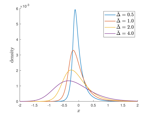
Figure 1. KoBoL estimated densities for several values of $\bar{\Delta}$ and Test I parameters in (5.2).

5.1. Density Estimation and FFT Aliasing

We start by demonstrating a primary deficiency of the FFT when estimating the transition density, which is resolved by using the SINH method to compute the density coefficients. The issue is related to truncation of the density support. For the SINH method, this truncation results in just one source of error, namely the loss of mass of the density, outside of the truncation interval. The coefficients are not otherwise impacted. By contrast, the FFT is subject to an additional source of error, in that the truncation of the density can actually reduce the accuracy of the computed coefficients near the boundaries the truncated support, as we illustrate in more detail below.

Figure 1 shows the KoBoL transition densities (plotted in log-space) with parameters in (5.2), computed using SINH for several values of the time step-size $\bar{\Delta}$. The densities exhibit an especially heavy right tail, due to $\lambda_{+}>|\lambda_{-}|$, with marked asymmetry. When using the FFT to compute coefficients (or other related computations), the well known aliasing effect emerges because, in effect, FFT replaces a given function by a periodic one, which reduces the accuracy of the computed coefficients. In particular, it is the slow tail decay, coupled with tail asymmetry, that causes difficulties when using the FFT. The left panel of Figure 2 demonstrates this problem. Since the left tail is much heavier than the right, the implied periodicity causes a loss of accuracy for coefficients near the left boundary.

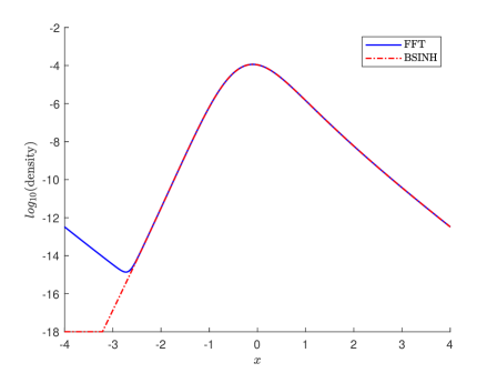
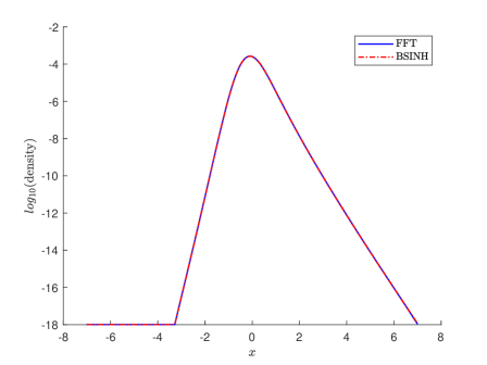
Figure 2. Visualization of aliasing effect in terms of log density using Test I parameters in (5.2), and $\bar{\Delta}=1$. Left: Density is truncated to the support $[-4,4]$, which fails to cover the mass in right tail. The heavy right tail causes aliasing of FFT on the left tail, due to assumed periodicity of FFT. Right: Removal of aliasing by increasing support to $[-7,7]$ to cover heavy right tail.

Naturally, the aliasing issue can be resolved by expanding the truncated density support, in this case from $[-4,4]$ to $[-7,7]$ (after experimentation), as illustrated in the right panel of Figure 2. There are two issues with this. The first is that we don’t know in advance that $[-7,7]$ is sufficient, and while it can be determined automatically by detecting aliasing effects after coefficient computation, this adds additional cost and complexity to the procedure. The second issue is that even if we can automatically determine a sufficiently wide truncation interval to avoid aliasing effects, it is wasteful of computational resources to extend the truncation grid just to avoid aliasing. Extending the grid width spreads out our $N_{x}$ basis elements, reducing the accuracy of the estimates (or equivalently the cost to achieve comparable accuracy).

5.2. European Options

The first set of experiments demonstrated the problem with the FFT when estimating the transition coefficients. Here we show the consequences this can have on our pricing accuracy for European options. We further demonstrate the robustness of SINH to mispecifying the truncated density support. For illustration, we consider the procedure introduced in Fang and Oosterlee, (2008), which recommends choosing the truncation half-width according to

(5.5) $$\alpha:=L_{1}\sqrt{|c_{2}|T+\sqrt{|c_{4}|T}},$$

where $c_{n}$ denotes the $n$-th cumulant of $\ln(S_{1}/S_{0})$, $T$ is the contract maturity, and $L_{1}$ is a user-supplied parameter. While simple to implement, this procedure requires the subjective choice of the parameter $L_{1}$, which can have a great impact on accuracy.

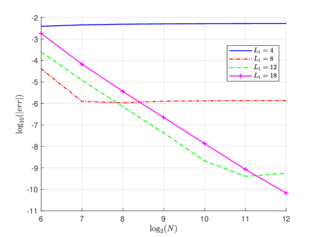
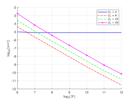
Figure 3. Robustness of SINH compared with FFT for mis-specification of truncated density support, with KoBoL Test I parameters in 5.2. European option price convergence with linear projection coefficients determined by FFT (Left) and SINH (right).

We next show that this impact can be amplified by the use of the FFT, whereas SINH is more robust. Figure 3 demonstrates the convergence in $N$ for a European call option, with $S_{0}=W=100$, $T=1$. Comparing the left and right panels, which show the convergence with coefficients obtained via the FFT and SINH, respectively, we see that SINH is more accurate for small values of $L_{1}$. Even with $L_{1}=4$, SINH easily achieves beyond practical precision. Since the full density width is $2\alpha$, this suggests that we can use many fewer basis elements with SINH to achieve the same level of accuracy.

	$L_{1}=4$				$L_{1}=8$
	FFT		SINH		FFT		SINH
$log_{2}(N_{y})$	Price	$|\text{Error}|$	Price	$|\text{Error}|$	Price	$|\text{Error}|$	Price	$|\text{Error}|$
5	0.83166761	5.82e-04	0.83163089	5.45e-04	0.83386326	2.78e-03	0.83390363	2.82e-03
6	0.83116978	8.40e-05	0.83115683	7.10e-05	0.83163074	5.45e-04	0.83163072	5.45e-04
7	0.83110239	1.66e-05	0.83108898	3.18e-06	0.83115681	7.10e-05	0.83115681	7.10e-05
8	0.83109959	1.38e-05	0.83108594	1.45e-07	0.83108896	3.16e-06	0.83108895	3.16e-06
9	0.83109758	1.18e-05	0.83108582	2.42e-08	0.83108592	1.25e-07	0.83108591	1.21e-07
10	0.83109762	1.18e-05	0.83108581	1.90e-08	0.83108580	8.90e-09	0.83108580	5.75e-09

Table 1. UOC barrier option converge, with $K=S_{0}=100$, $M=12$, $T=1.0$, and upper barrier $U=120$. KoBoL Test I parameters in (5.2).

5.3. Single Barrier Options

We next consider the case of barrier options, to demonstrate that the SINH approach can also be used to improve the computational performance of path-dependent pricing under the PROJ method. The first example we consider is that of an up-and-out call (UOC) option, with $T=1$ year to maturity, $M=12$ monitoring dates (monthly), struck at-the-money ($K=S_{0}=100$), with an upper barrier level at $U=120$. For convenience, we continue to use formula (5.5) to determine the truncation width of the density, which is parameterized by $L_{1}$. This allows us to directly control the truncation width, and demonstrate the loss in accuracy that occurs if the truncation width is chosen too small.

	$L_{1}=4$				$L_{1}=8$
	FFT		SINH		FFT		SINH
$log_{2}(N_{y})$	Price	$|\text{Error}|$	Price	$|\text{Error}|$	Price	$|\text{Error}|$	Price	$|\text{Error}|$
5	2.52550469	1.40e-02	2.52544628	1.39e-02	2.82699044	3.15e-01	2.79932530	2.88e-01
6	2.51273033	1.19e-03	2.51271077	1.17e-03	2.52548647	1.39e-02	2.52544624	1.39e-02
7	2.51158699	4.32e-05	2.51156667	2.29e-05	2.51271072	1.17e-03	2.51271073	1.17e-03
8	2.51157097	2.72e-05	2.51154362	1.20e-07	2.51156663	2.29e-05	2.51156663	2.29e-05
9	2.51157536	3.16e-05	2.51154382	8.44e-08	2.51154356	1.82e-07	2.51154355	1.88e-07
10	2.51157550	3.18e-05	2.51154383	8.93e-08	2.51154375	6.65e-09	2.51154374	1.65e-09

Table 2. DOP barrier option convergence, with $K=105,S_{0}=100$, $M=24$, $T=1.0$, and lower barrier $L=80$. KoBoL Test I parameters in (5.2).

Table 1 illustrates the convergence of FFT and SINH in the case of $L_{1}=4$ and $L_{1}=8$, as a function of the number of value grid points $N_{y}$. When $L_{1}=4$, we have clearly underspecfied the truncation width, and the FFT method ceases to improve in accuracy beyond $3e-05$, while SINH reaches $9e-08$ for the same width. As for the European case, by increasing $L_{1}$ we can achieve comparable accuracy with the FFT method, but a greater computational cost. In particular, doubling $L_{1}$ doubles the overall algorithm cost. We perform another experiment for a down-and-out put (DOP) option in Table 2 with Test I parameters, and in Table 3 with Test II parameters, where we observe similar results to the UOC example.

	$L_{1}=4$				$L_{1}=8$
	FFT		SINH		FFT		SINH
$log_{2}(N_{y})$	Price	$|\text{Error}|$	Price	$|\text{Error}|$	Price	$|\text{Error}|$	Price	$|\text{Error}|$
5	2.79848853	1.46e-04	2.79809624	2.47e-04	2.69181661	1.07e-01	2.70127090	9.71e-02
6	2.79825515	8.78e-05	2.79824741	9.55e-05	2.79848275	1.40e-04	2.79809618	2.47e-04
7	2.79833286	1.01e-05	2.79832651	1.64e-05	2.79824967	9.33e-05	2.79824740	9.55e-05
8	2.79835392	1.10e-05	2.79834147	1.47e-06	2.79832311	1.98e-05	2.79832651	1.64e-05
9	2.79835750	1.46e-05	2.79834294	2.16e-09	2.79834115	1.79e-06	2.79834147	1.47e-06
10	2.79835747	1.45e-05	2.79834296	1.47e-08	2.79834295	1.88e-09	2.79834294	6.26e-10

Table 3. DOP barrier option converge, with $K=100,S_{0}=100$, $M=6$, $T=0.5$, and lower barrier $L=80$. KoBoL Test II parameters in (5.3).

5.4. Double Barrier Options

Finally, we consider the case of a double barrier option. Unlike a single barrier (which has a semi-infinite continuation domain), the double barrier option price depends only on the density coefficients that overlap the compact interval $[L,U]$. Hence, only those coefficients should be computed before performing the convolution steps. For SINH, this is not a problem, while for FFT it leads to serious loss of accuracy due to aliasing, particularly when $[L,U]$ is narrow. The remedy proposed in Algorithm 4 of Kirkby, 2017a is to compute the coefficients by FFT over an enlarged interval, and restrict the convolution to those coefficients over $[L,U]$. This increases the cost of initialization, while the remaining computational cost for the convolution steps is unchanged. We refer to this anti-aliasing FFT approach as FFT-AA. Note that FFT-AA is a simplified version of the refined FFT technique developed and used in Boyarchenko and Levendorskiĭ, (2009, 2012) in Carr’s randomization algorithm (essentially, method of lines) applied to price barrier options with continuous monitoring.

	SINH			FFT		FFT-AA
$log_{2}(N_{y})$	Price	$|\text{Error}|$	Rate	Price	$|\text{Error}|$	Price	$|\text{Error}|$	NX
3	0.68580761	1.27e-03	–	0.68804791	3.51e-03	0.68580776	1.27e-03	6
4	0.68462085	8.05e-05	3.98	0.68811821	3.58e-03	0.68462085	8.05e-05	6
5	0.68454314	2.83e-06	4.83	0.68886527	4.32e-03	0.68454314	2.83e-06	6
6	0.68454041	1.02e-07	4.80	0.68933390	4.79e-03	0.68454041	1.02e-07	6
7	0.68454031	4.25e-09	4.58	0.68958569	5.05e-03	0.68454031	4.25e-09	6
8	0.68454031	3.14e-10	3.76	0.68971588	5.18e-03	0.68454031	3.12e-10	6

Table 4. Double barrier call option convergence, with $K=S_{0}=100$, $M=12$, $T=1.0$, barriers $[L,U]=[80,120]$. KoBoL Test I parameters in (5.2).

Table 4 displays the convergence results for a double barrier call option with $K=S_{0}=100$ and $[L,U]=[80,120]$ using Test I parameters. First we compare SINH with “naive FFT”, which computes the density coefficients corresponding to $[L,U]$ only. As expected the accuracy of FFT is capped (here at $e-03$), while PROJ with SINH converges nicely. Since SINH is not subject to truncation error, we are able to see the natural convergence rate of PROJ (with coefficients computed accurately) when only the projection error is present. The column “Rate” documents the rate of convergence corresponding to the SINH prices, computed as $-\log_{2}(\text{Error}_{k}/\text{Error}_{k-1})$. While the theoretical convergence of the linear basis is only second order, in practice we observe slightly better than fourth order convergence on average, as shown here for the double barrier option.

	SINH			FFT		FFT-AA
$log_{2}(N_{y})$	Price	$|\text{Error}|$	Rate	Price	$|\text{Error}|$	Price	$|\text{Error}|$	NX
3	0.09238632	2.44e-04	–	0.10436047	1.22e-02	0.09231996	1.78e-04	6
4	0.09214933	6.93e-06	5.14	0.10954382	1.74e-02	0.09214752	5.12e-06	6
5	0.09214327	8.66e-07	3.00	0.11281405	2.07e-02	0.09214339	9.81e-07	6
6	0.09214264	2.30e-07	1.91	0.11461655	2.25e-02	0.09214264	2.35e-07	6
7	0.09214243	2.36e-08	3.29	0.11556216	2.34e-02	0.09214243	2.01e-08	6
8	0.09214241	9.53e-11	7.95	0.11604647	2.39e-02	0.09214241	2.15e-10	6

Table 5. Double barrier put option convergence, with $K=S_{0}=100$, $M=12$, $T=1.0$, barriers $[L,U]=[90,110]$. KoBoL Test II parameters in (5.3).

We also compare PROJ with the FFT-AA approach, which after extending the coefficients during initialization, is able to remove the aliasing effects, and has a similar convergence rate to SINH. The column “NX” records the multiple of additional coefficients that are computed by FFT-AA compared with SINH during initialization, which is a 6 fold increase required to remove the aliasing effect. Hence, while the aliasing can be removed in this manner, it is computationally wasteful compared with SINH. Table 5 performs a similar experiment, for a double barrier put options, with narrower boundaries $[L,U]=[90,110]$, and Test II parameters. Again we see the computational improvement offered by SINH in eliminating the truncation error, and reducing the computational cost.

6. Conclusion

In the paper, we clarified relative advantages/disadvantages of different Fourier-based approaches to option pricing, and improved the B-spline density projection method using the sinh-acceleration technique to evaluate the projection coefficients. This allows one to completely separate the control of errors of the approximation of the transition operator at each time step as a convolution operator whose action is realized using the fast discrete convolution algorithm, and errors of the calculation of the elements of the discretized pricing kernel. The latter elements are calculated one-by-one (the procedure admits an evident parallelization), without resorting to FFT technique. Instead, appropriate conformal deformations of the contour of integration in the formula for the elements, with the subsequent change of variables, are used to greatly increase the rate of convergence. The changes of variables are such that the new integrand is analytic in a strip around the line of integration, hence, the integral can be calculated with accuracy E-14 to E-15 using the simplified trapezoid rule with a moderate or even small number of points. We explained the difficulties for accurate calculations of the coefficients using the FFT technique. Crucially, the use of the same pair of dual grids for all purposes, which is presented in many publications as a great advantage of the FFT technique, inevitably produces large errors unless extremely long grids are used. Furthermore, in some cases, even extremely long grids may be insufficient. We illustrated the advantages of the sinh-acceleration in the application to calculation of the B-spline coefficients through a series of numerical applications.

We also explained that although the spectral filtering technique allows one to increase the speed of calculations, spectral filters are designed to regularize the results. In applications to derivative pricing, the regularization results in serious errors in regions of the paramount importance for risk management: near barrier and strike, close to maturity and for long dated options, hence, ad-hoc choices of spectral filters can produce unacceptable errors. The approximations in the method of this paper also can be interpreted as spectral filters but the rigorous error bounds allow one to ensure the accuracy of the result, and the resulting error converges quickly (fourth order on average) as the approximation grid is refined.

As the first applications of the B-spline projection method with the improved procedure for the calculation of the coefficients, we considered the pricing of European as well as single and double barrier options with discrete monitoring, using backward induction in the state space. We list several sets of error bounds used in the literature, and discussed their relative advantages/disadvantages. The numerical experiments show that the use of SINH acceleration eliminates a key source of error in the B-spline projection methodology, which originates from the FFT when computing basis coefficients. By instead using the SINH method, the results are considerably more robust to under-specifying the density truncation width, for which aliasing of the FFT causes a deterioration of accuracy due to the assume periodicity of the FFT. While the aliasing effect can be removed with the FFT by increasing the grid width (sometimes substantially), doing so is computationally wasteful. The use of SINH acceleration allows the user to price options with a reduced truncation width at a commensurate reduction in computational effort, with added robustness to the choice of truncation width. For illustrative purposes, we focused on the case of European and Barrier options, but the proposed methodology extends naturally to other cases for which the PROJ method has been applied, such as for problems in risk management and insurance Wang and Zhang, (2019); Shi and Zhang, (2021); Zhang et al., (2020); Kirkby and Nguyen, (2021). The development of an improved procedure for basis coefficient calculation is beneficial across a variety of existing and future applications.

Appendix A Coefficient Formulas for Barrier Options

A.1. Down-and-Out Put Coefficients

The value coefficients for the DOP contract, $\theta^{DOP}_{M,k}=\theta_{M,k}$, are determined in closed form for the terminal (initializing) period, using the formulas derived in Kirkby, 2017a , to which we refer the reader for more details. Here we summarize the basic formulas, which can be combined with Algorithm 1 to price barrier options. First recall that the terminal DOP payoff is given by $(K-S_{0}e^{y})\mathbbm{1}_{[\ln(L/S_{0}),\ln(K/S_{0})]}(y).$ The nearest grid point left of $\ln(K/S_{0})$ is given by

(A.1) $$\bar{n}:=\lfloor(a\cdot(\ln(K/S_{0})-x_{1})+1\rfloor,$$

and the difference and normalized difference are defined by

(A.2) $$\rho:=\ln(K/S_{0})-x_{\bar{n}},\qquad\zeta:=a\cdot\rho.$$

Let

(A.3) $$b_{3}:=\sqrt{15},\quad b_{4}:=\sqrt{15}/10,$$

and

(A.4) $$\vartheta_{[-1,0]}\approx\frac{e^{-\Delta/2}}{18}\left(5\cosh(b_{4}\Delta)+b_{3}\sinh(b_{4}\Delta)+4\right),$$

(A.5) $$\vartheta_{[0,1]}\approx\frac{e^{\Delta/2}}{18}\left(5\cosh(b_{4}\Delta)-b_{3}\sinh(b_{4}\Delta)+4\right).$$

Set

(A.6) $$\vartheta^{*}:=\vartheta_{[-1,0]}+\vartheta_{[0,1]}.$$

Using the constants defined in Table 6, we have the formula

(A.7) $$\theta^{DOP}_{M,k}=\begin{dcases}\frac{K}{2}-L\cdot\vartheta_{[0,1]},&\mbox{ }k=1\\ K-e^{y_{k}}\cdot S_{0}\cdot(\vartheta_{[-1,0]}+\vartheta_{[0,1]}),&\mbox{ }k=2,...,\bar{n}-1\\ K\left(\frac{1}{2}+\bar{\delta}_{0}^{put}-e^{-\rho}\left(\vartheta_{[-1,0]}+\delta_{0}^{put}\right)\right),&\mbox{ }k=\bar{n}\\ K\left(\bar{\delta}_{1}^{put}-e^{\Delta-\rho}\cdot\delta_{1}^{put}\right),&\mbox{ }N_{y}=\bar{n}+1\\ 0,&\mbox{ }k=\bar{n}+2,...,N_{y}.\end{dcases}$$

A.2. Down-and-Out Call Coefficients

We next describe the formulas for DOC payoff coefficients. Define $\bar{n},\rho,\zeta$ as in equations (A.2) and (A.1), and further

(A.8) $$\sigma:=1-\zeta,\qquad\sigma_{\pm}:=\sigma(q_{\pm}-1/2)=\pm\frac{\sigma}{2}\sqrt{3/5},$$

(A.9) $$q_{-}:=\frac{1}{2}\left(1-\sqrt{3/5}\right),\qquad q_{+}:=\frac{1}{2}\left(1+\sqrt{3/5}\right).$$

Coefficients corresponding to the points $x_{\bar{n}}$ and $x_{\bar{n}+1}$ are affected by the grid misalignment (i.e., not all payoff singularities/kinks align with grid points), so we introduce the following integrals:

(A.10) $$\bar{\delta}_{0}^{call}:=\int_{1-\sigma}^{1}\varphi(y)dy,\qquad\delta_{0}^{call}:=\int_{1-\sigma}^{1}\varphi(y)e^{\frac{y}{a}}dy$$

(A.11) $$\bar{\delta}_{1}^{call}:=\int_{-\sigma}^{0}\varphi(y)dy,\qquad\delta_{1}^{call}:=\int_{-\sigma}^{0}\varphi(y)e^{\frac{y}{a}}dy.$$

Taking $\delta^{call}_{0}$ as an example, we apply the Gaussian quadrature approximation

$$\delta^{call}_{0} \approx\frac{\sigma}{18}\left[5\cdot\left((\sigma/2-\sigma_{-})e^{\Delta\sigma_{-}}+(\sigma/2-\sigma_{+})e^{\Delta\sigma_{+}}\right)+4\sigma\right]$$

$$=e^{\frac{\rho+\Delta}{2}}\frac{\sigma^{2}}{18}\left[5\cdot\left((1-q_{-})e^{\Delta\sigma_{-}}+(1-q_{+})e^{\Delta\sigma_{+}}\right)+4\right],$$

and similarly for $\delta^{call}_{1}$. The coefficients for $\bar{\delta}_{0}^{call},\bar{\delta}_{1}^{call}$ are derived exactly. Table 6 collects the resulting approximation formulas. The DOC coefficients are given by

(A.12) $$\theta^{DOC}_{M,k}=\begin{dcases}0&\mbox{ }k=1,\ldots,\bar{n}-1\\ K\left(\delta_{0}^{call}e^{-\rho}-\bar{\delta}_{0}^{call}\right)&\mbox{ }k=\bar{n}\\ K\left(e^{\Delta-\rho}\left(\vartheta_{[0,1]}+\delta_{1}^{call}\right)-\left(1/2+\bar{\delta}_{1}^{call}\right)\right)&\mbox{ }k=\bar{n}+1\\ S_{0}\exp(y_{k})\cdot\vartheta_{*}-K&\mbox{ }k=\bar{n}+2,...,N_{y}\end{dcases}$$

A.3. Up and Out Contracts

For UOC options, with the exception of $\theta^{UOC}_{M,N_{y}}$, the coefficients are identical to equation (A.12):

(A.13) $$\theta^{UOC}_{M,k}:=\begin{dcases}\theta^{DOC}_{M,k}&\mbox{ }k\leq N_{y}-1\\ U\cdot\vartheta_{[-1,0]}-W/2&\mbox{ }k=N_{y}.\end{dcases}$$

Similarly, for UOP options

(A.14) $$\theta^{UOP}_{M,k}=\begin{dcases}K-\exp(y_{k})S_{0}\cdot\vartheta_{*}&\mbox{ }k=1\\ \theta^{DOP}_{M,k}&\mbox{ }k=2,...,N_{y}\end{dcases}$$

where $\theta^{DOP}_{M,k}$ are defined in equation (A.7).

Gaussian Quadrature Adjustment for Payoff Coefficients
Puts	$\bar{\delta}_{j}^{put}$	$\delta_{j}^{put}$
$j=0$	$\zeta\left(1-\frac{1}{2}\zeta\right)$	$\frac{\zeta}{18}\left[4(2-\zeta)e^{\rho/2}+5\cdot\left((1-\zeta_{-})e^{\rho_{-}}+(1-\zeta_{+})e^{\rho_{+}}\right)\right]$
$j=1$	$\frac{\zeta^{2}}{2}$	$\frac{\zeta}{18}\cdot e^{-\Delta}\cdot\left[4\zeta\cdot e^{\rho/2}+5\left(\zeta_{-}e^{\rho_{-}}+\zeta_{+}e^{\rho_{+}}\right)\right]$
Calls	$\bar{\delta}_{j}^{call}$	$\delta_{j}^{call}$
$j=0$	$\frac{1}{2}+\zeta\left(\frac{\zeta}{2}-1\right)$	$e^{(\rho+\Delta)/2}\frac{\sigma^{2}}{18}\left[5\cdot\left((1-q_{-})e^{\Delta\sigma_{-}}+(1-q_{+})e^{\Delta\sigma_{+}}\right)+4\right]$
$j=1$	$\sigma-\frac{1}{2}\sigma^{2}$	$e^{(\rho-\Delta)/2}\frac{\sigma}{18}\cdot\left[4(\zeta+1)+5\left(\left(\frac{\zeta+1}{2}+\sigma_{-}\right)e^{\Delta\sigma_{-}}+\left(\frac{\zeta+1}{2}+\sigma_{+}\right)e^{\Delta\sigma_{+}}\right)\right]$

Table 6. Coefficients derived from a three point Gaussian quadrature.

Algorithm 1 Initialization by Automated Parameter Selection

1:Set $L_{1}\leftarrow 10;\quad$ Initialize $N$ as in Remark B.1

2:$\epsilon_{1}\leftarrow$5e-08; $\quad\epsilon_{2}\leftarrow$1e-05; $\quad\tau\leftarrow 1.1$

3:if Down-and-out: then

4:    $\alpha\leftarrow\max\Big{\{}\tau\cdot(\max\{0,\ln(W/S_{0})\}-l),\text{ }L_{1}\sqrt{c_{2}T+\sqrt{c_{4}T}}\Big{\}}$

5:    $x^{*}\leftarrow l+\alpha;\quad\Delta_{\xi}\leftarrow\pi(N-1)/(\alpha N)$

6:    while $|1-F_{\Delta_{\xi},N}(x^{*})|\cdot\max\{S_{0},W\}>\epsilon_{1}$ do

7:         $\alpha\leftarrow\tau\alpha;\quad N\leftarrow 2N;\quad x^{*}\leftarrow l+\alpha;\quad\Delta_{\xi}\leftarrow\pi(N-1)/(\alpha N)$

8:    end while

9:    $\mathcal{E}\leftarrow 2\mathcal{\epsilon}_{2};\quad N\leftarrow N/2$

10:    while $\mathcal{E}>\epsilon_{2}$ do

11:         $N\leftarrow 2N;\quad\Delta\leftarrow 2\alpha/(N-1);\quad n_{0}\leftarrow\lfloor 1-l/\Delta\rfloor$

12:         if $\Delta\leq l,\text{ }$ then $\Delta\leftarrow l/(1-n_{0})$ end if

13:         Use SINH to determine $\bm{\bar{\beta}}$.

14:         $\epsilon_{2}\leftarrow|E_{N}-\exp((r-q)\bar{\Delta})|\cdot M\quad$ ($E_{N}$ defined in equation (B.4))

15:    end while

16:else Up-and-out:

17:    $\alpha\leftarrow\max\Big{\{}\tau\cdot(u-\min\{0,\ln(W/S_{0})\}),\text{ }L_{1}\sqrt{c_{2}T+\sqrt{c_{4}T}}\Big{\}}$

18:    $x^{*}\leftarrow u-\alpha;\quad\Delta_{\xi}\leftarrow\pi(N-1)/(\alpha N)$

19:    while $|F_{\Delta_{\xi},N}(x^{*})|\cdot\max\{S_{0},W\}>\epsilon_{1}$ do

20:         $\alpha\leftarrow\tau\alpha;\quad N\leftarrow 2N;\quad x^{*}\leftarrow u-\alpha;\quad\Delta_{\xi}\leftarrow\pi(N-1)/(\alpha N)$

21:    end while

22:    $\mathcal{E}\leftarrow 2\mathcal{\epsilon}_{2};\quad N\leftarrow N/2$

23:    while $\mathcal{E}>\epsilon_{2}$ do

24:         $N\leftarrow 2N;\quad\Delta\leftarrow 2\alpha/(N-1);\quad n_{0}\leftarrow\lfloor N/2-u/\Delta\rfloor$

25:         if $\Delta\leq u,\text{ }$ then $\Delta\leftarrow u/(N/2-n_{0})$ end if

26:         Use SINH to determine $\bm{\bar{\beta}}$.

27:         $\epsilon_{2}\leftarrow|E_{N}-\exp((r-q)\bar{\Delta})|\cdot M\quad$ ($E_{N}$ defined in equation (B.4))

28:    end while

29:end if

30:return : $\bm{\bar{\beta}},\text{ }N,\text{ }\Delta,\text{ }\alpha,\text{ }n_{0}$

Appendix B Adaptive algorithm for Numerical Parameter Selection

There are two main parameters to choose when applying the PROJ algorithm. The first is $\alpha$, which specifies the truncated density support over $[-\alpha,\alpha]$. The location of the first grid point $x_{1}=-\alpha$. In general, $\alpha$ should be chosen to capture the mass of the transition density within some tolerance. Note that for double barrier options, $\alpha$ is determined by the barriers. The second parameter is $N_{x}$, which is the number of basis elements. Assuming that $\alpha$ is sufficiently large to control the truncation error, the convergence of the approximation to the price is determined by $N_{x}$.

Here we recollect the adaptive parameter selection algorithm proposed in Kirkby, 2017a for pricing single barrier options. The starting point is the selection of $\alpha$. With $L_{1}=10$, and fixing an initial $\widetilde{N}$ (see Remark B.1), we initialize $\alpha$ and $\Delta$ as $\widetilde{\alpha}$ and $\widetilde{\Delta}$, based on the contract maturity $T$:

(B.1) $$\widetilde{\alpha}=L_{1}\sqrt{T\cdot c_{2}+\sqrt{T\cdot c_{4}}},\qquad\widetilde{\Delta}=2\widetilde{\alpha}/(\widetilde{N}-1)$$

where $c_{2},c_{4}$ are the second and fourth cumulants of $\ln(S_{t+1}/S_{t})$ (see Fang and Oosterlee, (2008)). Once we have an initial choice of $\widetilde{\alpha}$, we update $\widetilde{\alpha}$ until it captures the mass of the density within a prescribed tolerance $\epsilon_{1}>0$, as follows. From Feng and Linetsky, (2008) we can represent the cumulative distribution of log return $Y_{T}=\ln(S_{T}/S_{0})$ by

$$F(x) =\int_{-\infty}^{x}p_{T}(y)dy=\int_{\mathbb{R}}p_{T}(y)\mathbbm{1}_{(-\infty,x)}dy$$

(B.2) $$=\mathcal{F}(\mathbbm{1}_{(-\infty,x)}\cdot p_{T})(0)=\frac{1}{2}-\frac{i}{2}\mathcal{H}(e^{-i\xi x}\phi_{T}(\xi))(0),$$

where $\mathcal{H}$ denotes the Hilbert transform

$$\mathcal{H}f(z)=\frac{1}{\pi}\text{PV}\int_{\mathbb{R}}\frac{f(y)}{z-y}dy.$$

Applied to equation (B.2), we have the discrete approximation

(B.3) $$F(x)\approx F_{\Delta_{\xi,N}}(x):=\frac{1}{2}+\frac{i}{2}\sum_{n=-(N-1)}^{N-1}\phi_{T}((n-\tfrac{1}{2})\Delta_{\xi})\frac{\exp(-ix(n-\tfrac{1}{2})\Delta_{\xi})}{(n-\tfrac{1}{2})\pi}.$$

We then estimate the probability mass of $\ln(S_{T}/S_{0})$ which is neglected by our grid choice, and increase the grid-width by a fixed multiplier $\tau>1$, until a probability tolerance $\epsilon_{1}>0$ is met. Moreover, since a grid for $\ln(S_{T}/S_{0})$ is much larger than required for any individual log return over an increment $\bar{\Delta}$, the truncation error for intermediate valuations is negligible.

For a down-and-out option, if the right tail estimate $|1-F_{\Delta_{\xi},N}(x_{N/2})|\cdot\max\{S_{0},W\}>\epsilon_{1}$, we double the grid size $N$, set $\alpha\leftarrow\tau\alpha$, and reestimate. For an up-and-out option, we similarly expand the grid as long as $|F_{\Delta_{\xi},N}(x_{1})|\cdot\max\{S_{0},W\}>\epsilon_{1}$, which estimates the error in the left tail. Note that in either case, we are only concerned with the probability within the continuation region.

In addition to controlling truncation error we utilize the martingale property of $e^{-(r-q)t}S_{t}$, namely $E[S_{t+\bar{\Delta}}|S_{t_{m}}]=S_{t_{m}}\exp((r-q)\bar{\Delta})$, to obtain a proxy for integration error incurred at each step:

(B.4) $$E_{N} :=\Upsilon_{a,N}\cdot\vartheta_{*}\cdot\sum_{n=1}^{N}\bar{\beta}_{n}\exp(x_{1}+(n-1)\Delta)$$

where $\vartheta_{*}$ is defined in (A.6). Here (B.4) approximates the expectation of log-return $\mathbb{E}[\exp(Y_{\bar{\Delta}})]=\exp((r-q)\bar{\Delta})$ using the projected density (calculated from $\phi_{\bar{\Delta}}$). In particular, the error in estimating $\bar{\beta}_{n}$, and our ability to accurately calculate intermediate value integrals, is reflected in equation (B.4). Hence, once the probability tolerance $\epsilon_{1}$ is satisfied, we further double the grid size as long as $|E_{N}-\exp((r-q)\bar{\Delta})|\cdot M>\epsilon_{2},$ where the multiplier $M$ accounts for the number of integral approximations made during the algorithm.

Remark B.1.

An initial starting value $N_{x}$ is required, which is initialized depending on $\bar{\Delta}=T/M$. For $\bar{\Delta}=1/100$ (which includes daily monitoring), we initialize $N_{x}\leftarrow 2^{10}$. Else if $\bar{\Delta}\leq 1/40$, we initialize $N_{x}\leftarrow 2^{9}$. Else, we initialize $N_{x}\leftarrow 2^{8}$.

In Algorithm 1, we set $\tau\leftarrow 1.1$, so at each stage the probability threshold is not satisfied, we increase the grid-width by ten percent. We set the tolerance thresholds $\epsilon_{1}\leftarrow$5e-08 and $\epsilon_{2}\leftarrow$1e-05 to conservatively achieve overall valuation error tolerance goal of TOL = 5e-04, which is sufficient for practical purposes. In general, a maximum value of $N$, for example $N=2^{17}$, should be enforced as a stopping criteria for automated parameter selection.

Appendix C Bounds for the interpolation and truncation errors

In this section, we list the error bounds and recommendations for the choice of the truncated interval and the discretization step derived in Innocentis and Levendorskiĭ, (2014). Let $\epsilon>0$ be the error tolerance, $X$ the Lévy process with the characteristic exponent $\psi$ admitting analytic continuation to a strip $\{\operatorname{\rm Im}\xi\in(\lambda_{-},\lambda_{+})\}$.

C.1. Truncation error

In the case of the double barrier options, no truncation is needed. Consider the down-and-out put option with the log-barrier $h=x_{1}$, strike $K$ and maturity $T$. In Innocentis and Levendorskiĭ, (2014) (Lemma 3.1 and Sect. 3.3.1), it is proved that, at the log-spot $x>h$, we minimize

(C.1) $$x_{M}=\frac{-(r+\psi(i\omega_{+}))T+\omega_{+}^{\prime}\ln K-\omega_{-}x+T(\psi(i\omega_{+})-\psi(i\omega_{-}))_{+}-\ln(\epsilon/K-e^{h})}{\omega_{+}-\omega_{-}}$$

over $\omega_{-}\in(\lambda_{-},0)$, $\omega_{+}\in(0,\lambda_{+})$, e.g., by using an optimization method such as conjugate gradient or Nelder-Mead. In the case of the down-and-out call option, one can make the Esscher transform thereby reducing to pricing an option with a payoff uniformly bounded by $K$. Trivially modifying the proof of Lemma 3.1 in Innocentis and Levendorskiĭ, (2014), one derives the following analog of (C.1), for down-and-out options with the payoffs bounded by $K$:

(C.2) $$x_{M}=\frac{-(r+\psi(i\omega_{+}))T-\omega_{-}x+T(\psi(i\omega_{+})-\psi(i\omega_{-}))_{+}-\ln(\epsilon/K)}{\omega_{+}-\omega_{-}}.$$

The case of the up-and-down call options is reducible to the case of the down-and-out put options by the change of measure and symmetry, and the case of up-and-out options with bounded payoffs to the case of down-and-out options by symmetry.

C.2. Interpolation error (discretization error in the state space)

Section 3.2 in Innocentis and Levendorskiĭ, (2014) contains the bounds and recommendations for options with uniformly bounded payoffs. To apply the results for call options, one has to change the measure and reduce to the case of the option with the bounded payoff. Lemma 3.2 in Innocentis and Levendorskiĭ, (2014) gives an error bound of the quadratic interpolation; for the cubic interpolation, see Levendorskiĭ and Xie, 2012b .

Lemma C.1.

Let $X$ be a Lévy process whose transition density $p_{\bar{\Delta}}$ satisfies $p_{\bar{\Delta}}\in C^{3}({\mathbb{R}})$ and $p^{(s)}_{\bar{\Delta}}\in L_{1}({\mathbb{R}}),s=1,2,3$, then the total error in the time-0 option price due to (piece-wise quadratic) interpolation admits the approximate bound via

$$\frac{e^{-rT}}{6}\Delta^{3}(N-1)(K-H)\|p_{\bar{\Delta}}^{{}^{\prime\prime\prime}}\|_{L_{1}}.$$

To apply Lemma C.1, one needs the following result (Proposition 3.3 in Innocentis and Levendorskiĭ, (2014)).

Lemma C.2.

Let $X$ be a model process of order $\nu>0$. Assume that $\nu$ and $\bar{\Delta}$ are not both small, and the mesh $\Delta$ is chosen so that the interpolation error of piece-wise quadratic interpolation is small. Then the following approximate bound holds

(C.3) $$\|p^{(n)}_{\bar{\Delta}}\|_{L_{1}}\leq\rho_{n},$$

where

(C.4) $$\rho_{n}=\frac{2\Gamma(n/\nu)}{(d_{+}^{0})^{n/\nu}\pi\nu D(n)}\bar{\Delta}^{-n/\nu},$$

and

(C.5) $$D(n)=\sup_{\phi\in\left(0,\min\{\frac{\pi}{2},\frac{\pi}{2\nu}\}\right)}(\cos(\phi\nu))^{n/\nu}\cos(\phi-\pi/2).$$

Applying Lemmas C.1-C.2, Section 3.2.1 in Innocentis and Levendorskiĭ, (2014) gives the following prescription:

(C.6) $$\Delta=\left(\frac{e^{-rT}}{6\epsilon}(N-1)(K-H)\rho_{3}\right)^{-\frac{1}{3}}.$$

Appendix D Auxiliary results

D.1. Programming convolution in MATLAB

We borrow this summary from Boyarchenko and Levendorskiĭ, (2009).

• Inputs: two arrays, $\vec{f}=(f_{j})_{j=1}^{M}$ and $\vec{g}=(g_{\ell})_{\ell=1-M}^{M-1}$ (in a program, the indices $\ell$ have to be shifted up).

• Output: the array $\vec{h}=(h_{k})_{k=1}^{M}$, whose entries are given by $h_{k}=\sum_{j=1}^{M}f_{j}g_{k-j}.$

• The calculation:

  $$\widetilde{g}=[\vec{g}(M:2*M-1)\quad 0\quad\vec{g}(1:M-1)];$$

  $$\widetilde{f}=[\vec{f}\quad\mathtt{zeros}(1,M)];$$

  $$\widetilde{h}=\mathrm{ifft}\left(\mathrm{fft}\widetilde{f}).*\mathrm{fft}(\widetilde{g})\right);$$

  $$\vec{h}=\widetilde{h}(1:M).$$

For agreement with MATLAB’s conventions, we assume that the array $\vec{g}$ is also indexed starting with $1$. Thus the first entry of $\vec{g}$ is $g_{1-M}$, and the $(2M-1)$-st entry is $g_{M-1}$.

MATLAB has a built-in conv function, which computes a certain version of the discrete convolution of two arrays. However, the realization of this function in MATLAB is also based on FFT, and typically, it is more convenient to use the algorithm presented above instead of conv.

References

- Abate and Valko, (2004) Abate, J. and Valko, P. (2004). Multi-precision Laplace inversion. International Journal of Numerical Methods in Engineering, 60:979–993.
- (2) Abate, J. and Whitt, W. (1992a). The Fourier-series method for inverting transforms of probability distributions. Queueing Systems, 10:5–88.
- (3) Abate, J. and Whitt, W. (1992b). Numerical inversion of of probability generating functions. Operation Research Letters, 12:245–251.
- Andricopoulos et al., (2003) Andricopoulos, A., Widdicks, D., Newton, D., and Duck, P. (2003). Universal option valuation using quadrature methods. J. Finan. Econ., 67:447–471.
- Barndorff-Nielsen, (1998) Barndorff-Nielsen, O. (1998). Processes of normal inverse Gaussian type. Finance and Stochastics, 2(1):41–68.
- Barndorff-Nielsen and Levendorskiǐ, (2001) Barndorff-Nielsen, O. and Levendorskiǐ, S. (2001). Feller Processes of Normal Inverse Gaussian type. Quantitative Finance, 1:318–331.
- Boyarchenko et al., (2011) Boyarchenko, M., de Innocentis, M., and Levendorskiĭ, S. (2011). Prices of barrier and first-touch digital options in Lévy-driven models, near barrier. International Journal of Theoretical and Applied Finance, 14(7):1045–1090. Available at SSRN: http://papers.ssrn.com/abstract=1514025.
- Boyarchenko and Levendorskiĭ, (2009) Boyarchenko, M. and Levendorskiĭ, S. (2009). Prices and sensitivities of barrier and first-touch digital options in Lévy-driven models. International Journal of Theoretical and Applied Finance, 12(8):1125–1170.
- Boyarchenko and Levendorskiĭ, (2012) Boyarchenko, M. and Levendorskiĭ, S. (2012). Valuation of continuously monitored double barrier options and related securities. Mathematical Finance, 22(3):419–444.
- Boyarchenko and Levendorskiĭ, (2015) Boyarchenko, M. and Levendorskiĭ, S. (2015). Ghost Calibration and Pricing Barrier Options and Credit Default Swaps in spectrally one-sided Lévy models: The Parabolic Laplace Inversion Method. Quantitative Finance, 15(3):421–441. Available at SSRN: http://ssrn.com/abstract=2445318.
- Boyarchenko and Levendorskiĭ, (1998) Boyarchenko, S. and Levendorskiĭ, S. (1998). On rational pricing of derivative securities for a family of non-Gaussian processes. Preprint 98/7, Institut für Mathematik, Universität Potsdam. Available at http://opus.kobv.de/ubp/volltexte/2008/2519/.
- Boyarchenko and Levendorskiĭ, (1999) Boyarchenko, S. and Levendorskiĭ, S. (1999). Generalizations of the Black-Scholes equation for truncated Lévy processes. Working Paper, University of Pennsylvania.
- Boyarchenko and Levendorskiĭ, (2000) Boyarchenko, S. and Levendorskiĭ, S. (2000). Option pricing for truncated Lévy processes. International Journal of Theoretical and Applied Finance, 3(3):549–552.
- Boyarchenko and Levendorskiĭ, (2002) Boyarchenko, S. and Levendorskiĭ, S. (2002). Non-Gaussian Merton-Black-Scholes Theory, volume 9 of Adv. Ser. Stat. Sci. Appl. Probab. World Scientific Publishing Co., River Edge, NJ.
- Boyarchenko and Levendorskiĭ, (2011) Boyarchenko, S. and Levendorskiĭ, S. (2011). New efficient versions of fourier transform method in applications to option pricing. Working paper. Available at SSRN: http://ssrn.com/abstract=1846633.
- Boyarchenko and Levendorskiĭ, (2013) Boyarchenko, S. and Levendorskiĭ, S. (2013). Efficient Laplace inversion, Wiener-Hopf factorization and pricing lookbacks. International Journal of Theoretical and Applied Finance, 16(3):1350011 (40 pages). Available at SSRN: http://ssrn.com/abstract=1979227.
- Boyarchenko and Levendorskiĭ, (2014) Boyarchenko, S. and Levendorskiĭ, S. (2014). Efficient variations of Fourier transform in applications to option pricing. J. Computational Finance, 18(2):57–90.
- Boyarchenko and Levendorskiĭ, (2017) Boyarchenko, S. and Levendorskiĭ, S. (2017). Efficient pricing barrier options and CDS in Lévy models with stochastic interest rate. Mathematical Finance, 27(4):1089–1123. DOI: 10.1111/mafi.12121.
- Boyarchenko and Levendorskiĭ, (2019) Boyarchenko, S. and Levendorskiĭ, S. (2019). SINH-acceleration: Efficient evaluation of probability distributions, option pricing, and Monte Carlo simulations. Int. J. Theoretical and Applied Finance, 22(2):49 pages.
- (20) Boyarchenko, S. and Levendorskiĭ, S. (2020a). Conformal accelerations method and efficient evaluation of stable distributions. Acta Applicandae Mathematicae, 169:711–765. Available at SSRN: https://ssrn.com/abstract=3206696 or http://dx.doi.org/10.2139/ssrn.3206696.
- (21) Boyarchenko, S. and Levendorskiĭ, S. (2020b). Static and semi-static hedging as contrarian or conformist bets. Mathematical Finance, 3(30):921–960. Available at SSRN: https://ssrn.com/abstract=3329694 or http://arxiv.org/abs/1902.02854.
- Briggs and Henson, (2005) Briggs, W. and Henson, V. (2005). The DFT: An Owners’ Manual for the Discrete Fourier Transform. SIAM, Philadelphia.
- Carr et al., (2002) Carr, P., Geman, H., Madan, D. B., and Yor, M. (2002). The fine structure of asset returns: an empirical investigation. J. Business, 75:305–332.
- Carr and Madan, (1999) Carr, P. and Madan, D. (1999). Option valuation using the Fast Fourier Transform. Journal of Computational Finance, 2(4):61–73.
- Carr and Madan, (2009) Carr, P. and Madan, D. (2009). Saddlepoint methods for option pricing. Journal of Computational Finance, 13(1):49–61.
- Christensen, (2003) Christensen, O. (2003). An Introduction to Frames and Riesz Bases. Birkhauser Boston.
- (27) Cui, Z., Kirkby, J., and Nguyen, D. (2017a). Equity-linked annuity pricing with cliquet-style guarantees in regime-switching and stochastic volatility models with jumps. Insurance: Mathematics and Economics, 74:46–62.
- (28) Cui, Z., Kirkby, J., and Nguyen, D. (2017b). A general framework for discretely sampled realized variance derivatives in stochastic volatility models with jumps. European J. Operational Research, 262(1):381–400.
- Cui et al., (2021) Cui, Z., Kirkby, J. L., and Nguyen, D. (2021). A data-driven framework for consistent financial valuation and risk measurement. European Journal of Operational Research, 289(1):381–398.
- Duffie et al., (2000) Duffie, D., Pan, J., and Singleton, K. (2000). Transform Analysis and Asset Pricing for Affine Jump Diffusions. Econometrica, 68:1343–1376.
- Duistermaat, (1995) Duistermaat, J. (1995). Fourier Integral Operators. Progress in Mathematics. Birkhäuser, Basel.
- Eskin, (1981) Eskin, G. (1981). Boundary Value Problems for Elliptic Pseudodifferential Equations, volume 9 of Transl. Math. Monogr. American Mathematical Society, Providence, RI.
- Eydeland, (1994) Eydeland, A. (1994). A fast algorithm for computing integrals in function spaces: financial applications. Computational Economics, 7:277–285.
- Eydeland and Mahoney, (2001) Eydeland, A. and Mahoney, D. (2001). The grid model for derivative pricing. Mirant Technical Report.
- Fang and Oosterlee, (2008) Fang, F. and Oosterlee, C. (2008). A novel pricing method for European options based on Fourier cosine series expansions. SIAM J. Sci. Comput., 31:826–848.
- Fedoryuk, (1987) Fedoryuk, M. (1987). Asymptotic: Integrals and Series. Nauka, Moscow. In Russian.
- Feng and Linetsky, (2008) Feng, L. and Linetsky, V. (July 2008). Pricing discretely monitored barrier options and defaultable bonds in Levy process models: a fast Hilbert transform approach. Math. Finan., 18(3):337–384.
- Fusai et al., (2006) Fusai, G., Abrahams, I., and Sgarra, C. (2006). An exact analytical solution for discrete barrier options. Finance and Stochastics, 10(1):1–26.
- Fusai et al., (2016) Fusai, G., Germano, G., and Marazzina, D. (2016). Spitzer identity, Wiener-Hopf factorization and pricing of discretely monitored exotic options. European Journal of Operational Research, 251(1):124–134. DOI:10.1016/j.ejor.2015.11.027.
- Gasquet and Witomski, (1998) Gasquet, C. and Witomski, P. (1998). Fourier Analysis and applications: filtering, numerical computation, wavelets. Springer, New York.
- Heil, (2011) Heil, C. (2011). A Basis Theory Primer. Birkhauser, expanded edition.
- Heston, (1993) Heston, S. (1993). A closed-form solution for options with stochastic volatility with applications to bond and currency options. Rev. Financ. Studies, 6:327–343.
- Hörmander, (1985) Hörmander, L. (1985). The Analysis of Linear Partial Differential Operators III: Pseudo-Differential Operators. Springer, Berlin.
- Innocentis and Levendorskiĭ, (2014) Innocentis, M. and Levendorskiĭ, S. (2014). Pricing discrete barrier options and credit default swaps under Lévy processes. Quantitative Finance, 14(8):1337–1365. Available at: DOI:10.1080/14697688.2013.826814.
- Innocentis and Levendorskiĭ, (2016) Innocentis, M. and Levendorskiĭ, S. (2016). Calibration and Backtesting of the Heston Model for Counterparty Credit Risk. Working paper. Available at SSRN: http://ssrn.com/abstract=2757008.
- Innocentis and Levendorskiĭ, (2017) Innocentis, M. and Levendorskiĭ, S. (2017). Calibration Heston Model for Credit Risk. Risk, pages 90–95.
- Kirkby, (2015) Kirkby, J. (2015). Efficient option pricing by frame duality with the fast Fourier transform. SIAM J. Financial Mathematics, 6(1):713–747.
- Kirkby, (2016) Kirkby, J. (2016). An efficient transform method for Asian option pricing. SIAM J. Financial Mathematics, 7(1):845–892.
- (49) Kirkby, J. (2017a). Robust barrier option pricing by frame projection under exponential Lévy dynamics. Applied Mathematical Finance, 24(4):337–386.
- (50) Kirkby, J. (2017b). Robust option pricing with characteristic functions and the B-spline order of density projection. J. Computational Finance, 21(2):101–127.
- Kirkby, (2018) Kirkby, J. (2018). American and exotic option pricing with jump diffusions and other Levy processes. J. Computational Finance, 22(3):89–148.
- (52) Kirkby, J. and Deng, S. (2019a). Static hedging and pricing of exotic options with payoff frames. Mathematical Finance, 29(2):612–658.
- (53) Kirkby, J. and Deng, S.-J. (2019b). Swing option pricing by dynamic programming with B-spline density projection. International Journal of Theoretical and Applied Finance, 22(08):1950038.
- Kirkby et al., (2017) Kirkby, J., Nguyen, D., and Cui, Z. (2017). A unified approach to Bermudan and barrier options under stochastic volatility models with jumps. J. Economic Dynamics and Control, 80:75–100.
- Kirkby et al., (2020) Kirkby, J. L., Mitra, S., and Nguyen, D. (2020). An analysis of dollar cost averaging and market timing investment strategies. European Journal of Operational Research, 286(3):1168–1186.
- Kirkby and Nguyen, (2021) Kirkby, J. L. and Nguyen, D. (2021). Equity-linked guaranteed minimum death benefits with dollar cost averaging. Insurance: Mathematics and Economics, 100:408–428.
- Kuznetsov, (2010) Kuznetsov, A. (2010). Wiener-Hopf factorization and distribution of extrema for a family of lévy processes. Annals of Applied Probability, 20:1801–1830.
- Lee, (2004) Lee, R. (2004). Option pricing by transform methods: extensions, unification, and error control. J. Comput. Finance, 7(3):50–86.
- Leentvaar and Oosterlee, (2008) Leentvaar, C. and Oosterlee, C. (2008). Multi-asset option pricing using a parallel Fourier-based technique. J. Comput. Fin., 12(1):1–26.
- Levendorskiĭ, (1993) Levendorskiĭ, S. (1993). Degenerate Elliptic Equations, volume 258 of Mathematics and its Applications. Kluwer Academic Publishers Group, Dordrecht.
- (61) Levendorskiĭ, S. (2004a). Early exercise boundary and option pricing in Lévy driven models. Quantitative Finance, 4(5):525–547.
- (62) Levendorskiĭ, S. (2004b). Pricing of the American put under Lévy processes. International Journal of Theoretical and Applied Finance, 7(3):303–335.
- Levendorskiĭ, (2012) Levendorskiĭ, S. (2012). Efficient pricing and reliable calibration in the Heston model. International Journal of Theoretical and Applied Finance, 15(7). 125050 (44 pages).
- Levendorskiĭ, (2014) Levendorskiĭ, S. (2014). Method of paired contours and pricing barrier options and CDS of long maturities. International Journal of Theoretical and Applied Finance, 17(5):1–58. 1450033 (58 pages).
- (65) Levendorskiĭ, S. (2016a). Fractional-Parabolic Deformations with Sinh-Acceleration. Working paper. Available at SSRN: http://ssrn.com/abstract=2758811.
- (66) Levendorskiĭ, S. (2016b). Pitfalls of the Fourier Transform method in Affine Models, and remedies. Applied Mathematical Finance, 23(2):81–134. Available at http://dx.doi.org/10.1080/1350486X.2016.1159918 or http://ssrn.com/abstract=2367547.
- Levendorskiĭ, (2018) Levendorskiĭ, S. (2018). Pricing arithmetic Asian options under Lévy models by backward induction in the dual space. SIAM FM, 9(1):1–27.
- (68) Levendorskiĭ, S. and Xie, J. (2012a). Fast pricing and calculation of sensitivities of OTM European options under Lévy processes. Journal of Computational Finance, 15(2). Available at SSRN:http://ssrn.com/abstract=1589809.
- (69) Levendorskiĭ, S. and Xie, J. (2012b). Pricing discretely sampled Asian options under Levy processes. Available at SSRN: http://papers.ssrn.com/abstract=2088214.
- Lord et al., (2008) Lord, R., Fang, F., Bervoets, F., and Oosterlee, C. (2008). A fast and accurate FFT-based method for pricing early-exercise options under Levy processes. SIAM J. Sci. Comput., 10:1678–1705.
- Madan and Seneta, (1990) Madan, D. and Seneta, E. (1990). The variance gamma (v.g.) model for share market returns. J. Business, 63:511–524.
- Madan et al., (1998) Madan, D. B., Carr, P., and Chang, E. (1998). The variance gamma process and option pricing. European Finance Review, 2:79–105.
- Ruijter et al., (2015) Ruijter, M., Versteegh, M., and Oosterlee, C. W. (2015). On the application of spectral filters in a fourier option pricing technique. Journal of Computational Finance, 19(1):75–106.
- Sato, (1999) Sato, K.-I. (1999). Levy Processes and Infinitely Divisible Distributions. Cambridge University Press, Cambridge, UK.
- Shi and Zhang, (2021) Shi, B. and Zhang, Z. (2021). Pricing EIA with cliquet-style guarantees under time-changed Levy models by frame duality projection. Comm. in Nonlinear Science and Numerical Sim., 95:105651.
- (76) Stenger, F. (1993a). Numerical Methods based on Sinc and Analytic functions. Springer-Verlag, New York.
- (77) Stenger, F. (1993b). Numerical Methods based on Sinc and Analytic functions. Springer-Verlag, New York.
- Stenger, (2000) Stenger, F. (2000). Summary of Sinc numerical methods. Journal of Computational and Applied Mathematics, 121:379–420.
- Unser and Daubechies, (1997) Unser, M. and Daubechies, I. (July 1997). On the approximation power of convolution-based least squares versus interpolation. IEEE Transactions on Signal Processing, 45(7):1697–1711.
- Wang and Zhang, (2019) Wang, W. and Zhang, Z. (2019). Computing the Gerber-Shiu function by frame duality projection. Scandanavian Actuarial Journal, 2019(4):291–307.
- Young, (1980) Young, R. (1980). An Introduction to Nonharmonic Fourier Series. Academic Press, New York, (revised) edition.
- Zhang et al., (2020) Zhang, Z., Yong, Y., and Yu, W. (2020). Valuing equity-linked death benefits in general exponential Lévy models. J. Computational and Applied Math., 365:112377.