Long-term evolution of neutron-star merger remnants in general relativistic resistive-magnetohydrodynamics with a mean-field dynamo term

Abstract

Long-term neutrino-radiation resistive-magnetohydrodynamics simulations in full general relativity are performed for a system composed of a massive neutron star and a torus formed as a remnant of binary neutron star mergers. The simulation is performed in axial symmetry incorporating a mean-field dynamo term for a hypothetical amplification of the magnetic-field strength. We first calibrate the mean-field dynamo parameters by comparing the results for the evolution of black hole-disk systems with viscous hydrodynamics results. We then perform simulations for the system of a remnant massive neutron star and a torus. As in the viscous hydrodynamics case, the mass ejection occurs primarily from the torus surrounding the massive neutron star. The total ejecta mass and electron fraction in the new simulation are similar to those in the viscous hydrodynamics case. However, the velocity of the ejecta can be significantly enhanced by magnetohydrodynamics effects caused by global magnetic fields.

I Introduction

The first observation of the binary neutron star merger GW170817 [1, 2] showed that theoretical modeling for the merger and post-merger phases of binary neutron stars is the key for extracting valuable information from the observed electromagnetic signals. Although there are a variety of the possibilities for the remnants of the binary neutron star mergers [3] and for the corresponding electromagnetic counterparts [4, 5], irrespective of the possibilities, the key phenomenon for the strong electromagnetic emission is the mass ejection from the remnant including the ultra-relativistic jets. Thus, the important aspect of the theoretical study is to clarify how the matter is ejected from the system and to understand the properties of the ejected matter such as total mass, typical velocity, and typical elements. This motivation has stimulated many numerical simulations for the merger phase (e.g., Refs. [6, 7, 8, 9, 10, 11, 12, 13, 14, 15, 16, 17]) and for the post-merger phase (e.g., Refs. [18, 19, 20, 21, 22, 25, 23, 24, 26, 27, 28, 29, 31, 30, 32, 33, 34, 35]) in the last decades.

For the binary neutron star merger resulting in the formation of a massive neutron star, the major mass ejection is likely to occur in the post-merger phase [16, 36] and the key process for the mass ejection from the merger remnant is the magnetohydrodynamical effect. For disks (or tori) surrounding the central compact object (either a massive neutron star or a black hole), which has approximately Keplerian rotational profile, it is believed that the magnetorotational instability (MRI) [37] is activated, and as a result, a turbulence is developed, enhancing the turbulence viscosity. The resulting viscous heating and angular momentum transport inevitably enhance the activity of the disk, and eventually, the mass ejection is induced. In addition, the amplified magnetic field could eventually develop a global magnetic field, which could further enhance the mass ejection efficiency [22, 27, 28, 35]. However, to fully clarify these processes, we need high-resolution simulations in three spatial dimension that can resolve the unstable modes of the MRI with a sufficient accuracy. However, to date, due to the limitation of the computational resource, such expensive simulations have not been performed yet (but see Ref. [38] for the high-resolution simulation to model accretion disks around a supermassive black hole).

The remnant massive neutron star also could be the source for the mass ejection [24, 31, 33, 34]. In contrast to the accretion disk around the compact objects, the angular velocity of the remnant massive neutron stars, $\Omega(\varpi)$ with $\varpi$ denoting the cylindrical radius, increases with $\varpi$ in the central region reflecting the nearly irrotational velocity field of the pre-merger stage of two neutron stars (e.g., Ref. [39]). Thus, the major region except for the outermost part of the remnant neutron star is stable to the MRI. However, there still exists the differential rotation in the remnant neutron star, which causes the winding of the magnetic field and increases the toroidal-field strength [40, 41, 42, 34]. In the presence of the resultant strong toroidal field, several magnetohydrodynamics (MHD) instabilities such as the Parker and Taylor instabilities [43, 44] together with the convection and circulation can take place, and the magnetic-field strength could be amplified through the dynamo action. To accurately investigate this amplification process, we need a high-resolution and long-term MHD simulation in full general relativity with the relevant microphysics such as the neutrino transport that can induce the convection and dynamo [45, 46]. However, this is still a formidable work in the current computational resources.

In this paper, we attack this problem phenomenologically, bypassing the high-resolution simulation. We perform general-relativistic neutrino-radiation resistive-MHD (GRRRMHD) simulations for a massive neutron star formed as a remnant of equal-mass binary neutron star mergers in axial symmetry as in our previous paper [34], but taking into account the mean-field dynamo term [47, 48, 34]; i.e., we incorporate the mean-field dynamo term in the current density $j^{\mu}$ which is proportional to the magnetic field. In the assumption of axial symmetry with no dynamo term, the poloidal magnetic field is not amplified even when the toroidal-field strength is significantly enhanced, due to the anti-dynamo property [49]. With the phenomenological incorporation of the dynamo term, by contrast, the poloidal magnetic field can be amplified in the presence of the toroidal field. As a result, the magnetic field continues to be amplified even if we start initially from a purely toroidal magnetic field in the axisymmetric simulation. In the context of the MHD evolution of the binary-neutron-star merger remnant, the differential rotation is likely to be the key for the magnetic-field amplification. Thus, we pay attention only to the $\alpha$-$\Omega$ dynamo for the hypothetical field amplification in this paper.

Similar numerical experiments in MHD have been recently performed by several groups [51, 50, 52, 53] for the systems of a black hole and a disk assuming the fixed back ground of the black hole. These works have illustrated that with the incorporation of the mean-field dynamo term (i.e., with the $\alpha$-$\Omega$ dynamo effect), the numerical results by the three-dimensional ideal MHD simulations are at least qualitatively reproduced. These results encourage us to perform this type of a phenomenological simulation to capture a realistic MHD evolution process of the remnant of the binary neutron star mergers, which cannot be currently studied in the first-principle MHD simulation due to the poor grid resolution resulting from the limitation of the computational resources. This type of the phenomenological simulations is also helpful to explore a wide variety of the possibilities for the long-term evolution process of the binary-neutron-star merger remnants, which have not been well explored yet, with a (relatively) inexpensive computational cost. In particular, to derive theoretical models for the ejecta with which electromagnetic signals are studied, the simulation results provide the useful data for the post-process calculations (see, e.g., Refs. [54, 55, 56]).

The paper is organized as follows: In Sec. II, we summarize the basic equations employed in the present numerical simulations paying particular attention to the resistive MHD equations in general relativity. In Sec. III we first calibrate our method by performing the simulations for the system of a black hole and a disk. We compare the results with those in viscous hydrodynamics [29, 30] and confirm that the new results by the GRRRMHD simulations are quantitatively similar to those by the previous viscous hydrodynamics simulations with an appropriate choice of the dynamo parameters, although the MHD effects can modify the process of the mass ejection. Then, in Sec. IV, we perform a GRRRMHD simulation for a remnant of a binary neutron star merger composed of a massive neutron star and a torus. By comparing the results with those by the viscous hydrodynamics simulation [31], we show additionally significant magnetohydrodynamics effects on the matter ejected from the system. Section V is devoted to a summary. Throughout this paper, we use the geometrical units of $c=1=G$ where $c$ and $G$ denote the speed of light and the gravitational constant, respectively (but $c$ is often recovered to clarify the units in the following sections). Latin and Greek indices denote the space and spacetime components, respectively. In Sec. II, we suppose to use Cartesian coordinates for the spatial components whenever equations are written.

II Basic equations for numerical computations

II.1 Brief summary

We perform a resistive MHD simulation in full general relativity using the same formulation and numerical implementation as in our previous paper [34] (see this reference for details of the formulation and numerical methods, and for the results of test-bed problems). Specifically, we numerically solve Einstein’s equation, resistive MHD equations incorporating a mean-field dynamo term, evolution equations for the lepton fractions including the electron fraction, and (approximate) neutrino-radiation transfer equations. Except for an MHD part (see the next paragraphs), the basic equations and input physics are the same as before: Einstein’s equation is solved using the original version of the Baumgarte-Shapiro-Shibata-Nakamura formalism [57] together with the puncture formulation [58], Z4c constraint propagation prescription [59], and 5th-order Kreiss-Oliger dissipation. The axial symmetry for the geometric variables is imposed using the cartoon method [60, 61] with the 4th-order accurate Lagrange interpolation in space. The lepton fractions are evolved taking into account electron and positron captures, electron-positron pair annihilation, nucleon-nucleon bremstrahlung, and plasmon decay [24, 31]. The same tabulated equation of state as in Refs. [29, 30, 34] is employed. Specifically, we employ the DD2 equation of state [62] for a relatively high-density part and the Timmes (Helmholtz) equation of state for a low-density part [63].

We evolve weighted electric and magnetic fields defined, respectively, by [64, 65, 34]

$${\cal{E}}^{\mu} := \sqrt{\gamma}F^{\mu\nu}n_{\nu},$$ (1)

$${\cal{B}}^{\mu} := {1\over 2}\sqrt{\gamma}n_{\alpha}\epsilon^{\alpha\mu\nu\beta}F_{\nu\beta},$$ (2)

where the electromagnetic tensor is written as

$$F^{\mu\nu}=n^{\mu}E^{\nu}-n^{\nu}E^{\mu}+n_{\beta}\epsilon^{\beta\mu\nu\alpha}B_{\alpha},$$ (3)

with $n^{\alpha}$ the time-like unit normal vector, $\gamma$ the determinant of the spatial metric $\gamma_{ij}$, and $\epsilon^{\mu\nu\alpha\beta}$ the Levi-Civita tensor. $E^{\mu}$ and $B^{\mu}$ are the electric and magnetic fields in the inertial frame, respectively.

The evolution equations for ${\cal{E}}^{i}$ and ${\cal{B}}^{i}$ are written as [34]

$$\partial_{t}{\cal{E}}^{i}=-\partial_{k}\left(\beta^{i}{\cal{E}}^{k}-\beta^{k}{\cal{E}}^{i}+\alpha\epsilon^{kij}{\cal{B}}_{j}\right)$$

$$~{}~{}~{}~{}~{}~{}~{}~{}~{}~{}~{}~{}-4\pi\left({\cal{J}}^{i}-Q\beta^{i}\right),$$ (4)

$$\partial_{t}{\cal{B}}^{i}=-\partial_{k}\left(\beta^{i}{\cal{B}}^{k}-\beta^{k}{\cal{B}}^{i}-\alpha\epsilon^{kij}{\cal{E}}_{j}\right)$$

$$~{}~{}~{}~{}~{}~{}~{}~{}~{}~{}~{}-\alpha\gamma^{1/2}\gamma^{ij}\partial_{j}\phi_{B}$$ (5)

$$\partial_{t}\phi_{B}=\beta^{k}\partial_{k}\phi_{B}-\alpha\kappa\phi_{B}-\alpha\gamma^{-1/2}\partial_{k}{\cal{B}}^{k},$$ (6)

where $\alpha$ is the lapse function, $\beta^{i}$ is the shift vector, $\epsilon^{kij}:=n_{\mu}\epsilon^{\mu kij}$, $\phi_{B}$ is a new auxiliary variable associated with the divergence cleaning, $\kappa$ is a constant, and the current term, ${\cal{J}}^{i}-Q\beta^{i}$, is written as [48, 51, 53, 34]

$${\cal{J}}^{i}-Q\beta^{i}=Qv^{i} + \alpha\sigma_{\rm c}\Big{[}wA^{i}_{~{}j}{\cal{E}}^{j}+\epsilon^{ijk}u_{j}{\cal{B}}_{k}$$ (7)

$$- \alpha_{\rm d}\left(-wA^{i}_{~{}j}{\cal{B}}^{j}+\epsilon^{ijk}u_{j}{\cal{E}}_{k}\right)\Big{]},$$

with $A^{i}_{~{}j}:=\delta^{i}_{~{}j}-w^{-2}\bar{u}^{i}u_{j}$, $\bar{u}^{i}=\gamma^{ij}u_{j}$, $u^{\mu}$ the four velocity, $v^{i}:=u^{i}/u^{t}$, and $w=\alpha u^{t}$. $Q$ is a weighted charge density evaluated by $\partial_{k}{\cal{E}}^{k}/4\pi$. $\sigma_{\rm c}$ is the conductivity ($\eta:=c^{2}/(4\pi\sigma_{\rm c})$ is the resistivity), and $\alpha_{\rm d}$ denotes the so-called $\alpha$-parameter that controls the mean-field dynamo [47, 48, 51, 52]. By normalizing it with respect to the speed of light, we consider $\alpha_{\rm d}$ as a dimensionless parameter in this paper. In contrast to the previous work [34], we always consider the cases of a non-zero value of $\alpha_{\rm d}$ in this paper. $\kappa$ is chosen to be $10^{5}\,{\rm s}^{-1}$ for all the simulations.

In the present context, we suppose that $\sigma_{\rm c}$ and $\alpha_{\rm d}$ should be determined by hypothetical turbulence motion of the fluid and resulting dynamo process. We phenomenologically give these parameters from the consideration for the plausible processes that play an important role in the remnant of binary neutron star mergers as well as in the accretion disk around a neutron star or a black hole.

II.2 Choice of $\sigma_{\rm c}$ and $\alpha_{\rm d}$

In the presence of non-zero values of $\alpha_{\rm d}$ and differential rotation, the so-called $\alpha$-$\Omega$ dynamo can be activated. In the non-relativistic case, the local analysis leads to the following dispersion relation for the wave mode of the form $\propto\exp(i\omega t-ik_{i}x^{i})$ [47]:

$$(i\omega+\eta k^{2})^{2}+i\alpha_{\rm d}S_{\Omega}k_{\parallel}c-\alpha_{\rm d}^{2}k^{2}c^{2}=0,$$ (8)

where $k^{2}=k_{i}k^{i}$, $S_{\Omega}:=\partial\Omega/\partial\ln\varpi$, and $k_{\parallel}$ denotes the wave number in the direction parallel to the rotational axis. To clarify the physical dimensions, $c$ is recovered in this subsection. The solution of Eq. (8) is written as

$$i\omega=-\eta k^{2}\pm\sqrt{\alpha_{\rm d}^{2}k^{2}c^{2}-i\alpha_{\rm d}S_{\Omega}k_{\parallel}c}.$$ (9)

In this paper, we pay attention only to the case that a large-scale dynamo plays a key role; i.e., we consider the case of $\alpha_{\rm d}^{2}k^{2}c^{2}\ll|\alpha_{\rm d}S_{\Omega}|k_{\parallel}c$. For this case, Eq. (9) is approximated as [47]

$$i\omega\approx-\eta k^{2}\pm{1-i\over\sqrt{2}}\sqrt{|\alpha_{\rm d}S_{\Omega}|k_{\parallel}c},$$ (10)

and thus, the condition for the presence of the unstable modes becomes $\sqrt{|\alpha_{\rm d}S_{\Omega}|k_{\parallel}c/2}>\eta k^{2}$. Focusing on the most optimistic case of $k^{2}=k_{\parallel}^{2}$, the condition for $k$ to give an unstable mode becomes

$$k < (8\pi^{2}\sigma_{\rm c}^{2}|\alpha_{\rm d}S_{\Omega}|)^{1/3}c^{-1}$$ (11)

$$= 6.4\times 10^{-6}\,{\rm cm}^{-1}\left({|\alpha_{\rm d}|\over 10^{-4}}\right)^{1/3}$$

$$\times\left({\sigma_{\rm c}\over 3\times 10^{7}\,{\rm s}^{-1}}\right)^{2/3}\left({|S_{\Omega}|\over 10^{3}\,{\rm rad/s}}\right)^{1/3},$$

and the wave number of the fastest growing mode is

$$k_{\rm fast} = \left({\pi^{2}\sigma_{\rm c}^{2}|\alpha_{\rm d}S_{\Omega}|\over 2}\right)^{1/3}c^{-1}$$ (12)

$$= 2.5\times 10^{-6}\,{\rm cm}^{-1}\left({|\alpha_{\rm d}|\over 10^{-4}}\right)^{1/3}$$

$$\times\left({\sigma_{\rm c}\over 3\times 10^{7}\,{\rm s}^{-1}}\right)^{2/3}\left({|S_{\Omega}|\over 10^{3}\,{\rm rad/s}}\right)^{1/3}.$$

For the dynamo instability to take place in the remnant neutron star, the typical scale of the unstable mode estimated broadly by $\sim\pi/(2k_{\rm fast})$ should not be larger than the radius of the neutron star $\sim 10$ km. Thus, the condition to get the dynamo instability in the neutron star becomes $\alpha_{\rm d}\sigma_{\rm c}^{2}\gtrsim 10^{10}\,{\rm s}^{-2}$.

For the fastest growing mode, the growth rate is written as

$$\omega_{\rm max} = {3\over 4}\left({\pi\alpha_{\rm d}^{2}\sigma_{\rm c}S_{\Omega}^{2}\over 4}\right)^{1/3}=46\,{\rm s}^{-1}\left({|\alpha_{\rm d}|\over 10^{-4}}\right)^{2/3}$$ (13)

$$\times\left({\sigma_{\rm c}\over 3\times 10^{7}\,{\rm s}^{-1}}\right)^{1/3}\left({|S_{\Omega}|\over 10^{3}\,{\rm rad/s}}\right)^{2/3}.$$

Thus, for massive neutron stars of mass $\sim 2.5M_{\odot}$ for which $|S_{\Omega}|$ is typically of $O(10^{3})\,{\rm rad/s}$, the growth timescale of the electromagnetic fields is of order $10$ ms. For accretion disks around a compact object of mass $\sim 3$–$10M_{\odot}$, $|S_{\Omega}|$ can be slightly smaller, but for a compact orbit of radius $\sim 100$ km, the growth timescale is also as short as $\sim 10^{2}$ ms. For an accretion disk which orbits far from the central object, $|S_{\Omega}|$ is smaller $\ll 10^{3}$ rad/s, and the timescale of the dynamo action is longer. Specifically, $|S_{\Omega}|$ is approximately proportional to $R_{\rm disk}^{-3/2}$ where $R_{\rm disk}$ denotes the typical radius of the accretion disk, and thus, $\omega_{\rm max}$ is approximately proportional to $R_{\rm disk}^{-1}$. This implies that for distant orbits, the dynamo action becomes inefficient, if the values of $\sigma_{\rm c}$ and $\alpha_{\rm d}$ for the non-compact disks are as large as those for the compact disks.

Equation (10) shows that in addition to the growth (or damping) the electromagnetic field oscillates with the angular frequency of

$$\omega_{\rm osc} := \sqrt{{|\alpha_{\rm d}S_{\Omega}|k_{\parallel}c\over 2}}=61\,{\rm s}^{-1}\left({|\alpha_{\rm d}|\over 10^{-4}}\right)^{1/2}$$ (14)

$$\times \left({|S_{\Omega}|\over 10^{3}\,{\rm rad/s}}\right)^{1/2}\left({k_{\parallel}\over 2.5\times 10^{-6}\,{\rm cm}^{-1}}\right)^{1/2}.~{}~{}~{}$$

Thus, with our choice of $\sigma_{\rm c}$ and $\alpha_{\rm d}$ (see below), the electromagnetic field changes the polarity with the period of the order of $0.1$ s($\sim 2\pi/\omega_{\rm osc}$) for the object of total mass $\sim 3M_{\odot}$ and longer for the larger mass.

In the quasi-linear approximation under the assumption of the isotropic turbulence [47], the turbulent transport coefficients, i.e., $\alpha_{\rm d}$ and $\eta$, are estimated by

$$\alpha_{\rm d}\approx-{1\over 3c}\tau_{\rm cor}\langle u_{i}\omega^{i}\rangle,$$ (15)

$$\eta\approx{1\over 3}\tau_{\rm cor}\langle u_{i}u^{i}\rangle,$$ (16)

where $\tau_{\rm cor}$ is a correlation time, $u_{i}$ is the fluctuation part of the spatial velocity, and $\omega^{i}=\epsilon^{ijk}\partial_{j}u_{k}$: the vorticity. $\langle\cdots\rangle$ denotes the ensemble averaging. Assuming that $u_{i}$ and $\tau_{\rm cor}$ are comparable to the Alfvén velocity and Alfvén timescale, the typical sizes for them are evaluated by

$$|u_{i}| \approx {B\over\sqrt{4\pi\rho}}=2.0\times 10^{7}\,{\rm cm/s}\left({B\over 10^{15}\,{\rm G}}\right)$$ (17)

$$~{}~{}~{}~{}~{}\times\left({\rho\over 2\times 10^{14}\,{\rm g\,cm^{-3}}}\right)^{-1/2},$$

$$\tau_{\rm cor} \approx {R\over|u_{i}|}=50\,{\rm ms}\left({R\over 10\,{\rm km}}\right)\left({B\over 10^{15}\,{\rm G}}\right)^{-1}$$ (18)

$$~{}~{}~{}~{}~{}\times\left({\rho\over 2\times 10^{14}\,{\rm g\,cm^{-3}}}\right)^{1/2},$$

where $B$ is the typical magnetic-field strength, $\rho$ is the rest-mass density, and $R$ is the radius of the neutron star. Assuming that the order of magnitude of $\omega^{i}$ is the same as that of $|u_{i}|/R$, we obtain $|\alpha_{\rm d}|=O(10^{-4})$ and $\eta=O(10^{12})$–$O(10^{13})\,{\rm cm^{2}/s}$, i.e., $\sigma_{\rm c}=O(10^{7})$–$O(10^{8})\,{\rm s}^{-1}$. For these values, the $\alpha$-$\Omega$ dynamo can be activated for long wavelength modes of $\gtrsim 1$ km (cf. Eq. (11)). In this paper, we broadly suppose the situation for which the remnant neutron star and torus (or disk) are unstable for the $\alpha$-$\Omega$ dynamo with these long wavelength modes.

For dense accretion disks/tori surrounding a black hole/neutron star which we consider in this paper, the typical sizes of $|u_{i}|$ and $\tau_{\rm cor}$ are smaller and larger than those in Eqs. (17) and (18), respectively. (We note that $R$ should be replaced by the geometrical thickness of the disk/torus which is $\lesssim 100$ km.) However, the order of the magnitude is not significantly different from those for the neutron star. Hence, we employ the same values of $\sigma_{\rm c}$ and $\alpha_{\rm d}$ both for the remnant neutron star and accretion disks surrounding the central compact objects for simplicity, while we perform several simulations varying these parameters for a certain range.

We note that in the late evolution stage of the remnant neutron star, the degree of the differential rotation is likely to become weak due to the MHD effects (cf. Sec. IV). Even for such a state, the magnetic-field amplification may be still preserved by the $\alpha$-dynamo, for which the necessary condition (from Eq. (9) with $S_{\Omega}=0$) is written as [47]

$$k<{4\pi\sigma_{\rm c}|\alpha_{\rm d}|\over c},$$ (19)

or equivalently

$$\lambda={2\pi\over k}>50\,{\rm km}\left({|\alpha_{\rm d}|\over 10^{-4}}\right)^{-1}\left({\sigma_{\rm c}\over 3\times 10^{7}\,{\rm s}^{-1}}\right)^{-1}.$$ (20)

Thus, with the setting of $\alpha_{\rm d}=10^{-4}$ and $\sigma_{\rm c}\lesssim 10^{8}\,{\rm s}^{-1}$, the wavelength for the unstable modes is so long that the effect of the $\alpha$-dynamo is minor. Hence, the magnetic field is likely to decay with the time scale of $\gtrsim 4\pi\sigma_{\rm c}/(kc)^{2}$ where $\sim k^{-1}$ denotes the curvature scale of the magnetic-field lines. In reality, in the absence of the differential rotation, a convection or turbulence is not likely to be preserved, and thus, supposing the mean-field dynamo is unlikely to be correct. Thus in this paper, we do not touch on the very late time evolution of the system, in which the magnetic-field decays due to the resistivity.

Finally we note that $\alpha_{\rm d}$ is not a pure scalar but an axial scalar because it has the same polarity as that of the toroidal magnetic field. In the simulation of this paper we assume the plane symmetry with respect to the equatorial plane. Thus, $\alpha_{\rm d}$ should have the reflection anti-symmetry for the change of $z\rightarrow-z$, and thus, $\alpha_{\rm d}=0$ on the $z=0$ (equatorial) plane. To impose this condition, we employ the functional form of $\alpha_{\rm d}$ as

$$\alpha_{\rm d}=\alpha_{\rm d,0}\left[{2\over\exp(-|z|/z_{\rm c})+1}-1\right]{z\over|z|},$$ (21)

where we choose $z_{\rm c}=0.5$ km in this paper, and $\alpha_{\rm d,0}$ is a constant chosen based on the estimate for the approximate magnitude of $\alpha_{\rm d}$ shown above (hereafter we denote $\alpha_{\rm d,0}$ simply by $\alpha_{\rm d}$). Since the value of $z_{\rm c}$ is much smaller than the geometrical thickness of the disk and radius of the neutron star, the dynamo effect is assumed to be present for a wide region in which the matter is present.

II.3 Diagnostics

We always calculate the following quantities for the simulation results: average specific entropy $\langle s\rangle$ and average electron fraction $\langle Y_{e}\rangle$ both for the matter located outside the black hole and for the ejecta (see the method for identifying the ejecta below). For the former case, these average quantities are defined by

$$\langle s\rangle := {1\over M_{\rm mat}}\int_{\rm out}\rho_{*}s\,d^{3}x,$$ (22)

$$\langle Y_{e}\rangle := {1\over M_{\rm mat}}\int_{\rm out}\rho_{*}Y_{e}\,d^{3}x,$$ (23)

where $M_{\rm mat}$ denotes the rest mass of the matter located outside the black hole, defined by

$$M_{\rm mat} := \int_{\rm out}\rho_{*}\,d^{3}x,$$ (24)

and $\int_{\rm out}$ implies that the volume integral is performed for the matter located outside the black hole. For the ejecta component, the volume integral is performed for the matter that satisfies the ejecta criterion (see below).

The kinetic energy and the electromagnetic energy of the system are defined by

$$E_{\rm kin} := {1\over 2}\int_{\rm out}\rho_{*}hu_{i}v^{i}d^{3}x,$$ (25)

$$E_{\rm B} := {1\over 8\pi}\int_{\rm out}(B^{2}+E^{2})\sqrt{-g}\,d^{3}x.$$ (26)

The ejecta component is determined using the same criterion as in Refs. [29, 31]; we identify a matter component with $|hu_{t}|>h_{\rm min}$ located in a far region as the ejecta. Here $h_{\rm min}$ denotes the minimum value of the specific enthalpy in the adopted equation-of-state table, which is $\approx 0.9987c^{2}$. For the matter escaping from a sphere of its radius $r=r_{\rm ext}$, we define the ejection rates of the rest mass and energy (kinetic energy plus internal energy) at a given radius and time by

$$\dot{M}_{\rm eje} := \oint\rho\sqrt{-g}u^{i}dS_{i},$$ (27)

$$\dot{E}_{\rm eje} := \oint\rho\hat{e}\sqrt{-g}u^{i}dS_{i},$$ (28)

where $\hat{e}:=h\alpha u^{t}-P/(\rho\alpha u^{t})$. The surface integral is performed at $r=r_{\rm ext}$ with $dS_{i}=\delta_{ir}r_{\rm ext}^{2}\sin\theta d\theta d\varphi$ for the ejecta component. $r_{\rm ext}$ is chosen to be $\approx 6000$ km for black hole-disk systems (with the mass of the black hole of $10M_{\odot}$) and 1500 km for neutron star-torus systems in this work.

As in our previous paper [34], the total rest mass and energy (excluding the gravitational potential energy and electromagnetic energy) of the ejecta (which escape away from a sphere of $r=r_{\rm ext}$) are calculated, respectively, by

$$M_{\rm eje}(t) := \int^{t}\dot{M}_{\rm eje}dt,$$ (29)

$$E_{\rm eje}(t) := \int^{t}\dot{E}_{\rm eje}dt.$$ (30)

Far from the central object, $E_{\rm eje}$ is approximated by the sum of the rest-mass energy and kinetic energy, as we discussed in Ref. [34]. Since the ejecta velocity can be relativistic in this work, we first define an average Lorentz factor of the ejecta (for the component that escapes from a sphere of $r=r_{\rm ext}$) by

$$\Gamma_{\rm eje}:=\sqrt{{E_{\rm eje}-GMM_{\rm eje}/r_{\rm ext}\over M_{\rm eje}c^{2}}},$$ (31)

where $M$ denotes the total gravitational mass of the system and $G$ is recovered to clarify that the last term in the numerator of Eq. (31) approximately denotes the gravitational potential energy of the matter at $r=r_{\rm ext}$. Finally, the average ejecta velocity is calculated by $v_{\rm eje}:=\sqrt{1-\Gamma_{\rm eje}^{-2}}$.

III Evolution of black hole-disk systems

III.1 Setup

First we evolve systems composed of a spinning black hole and a disk surrounding it. We employ the same initial conditions as models M10L05 and M10H05 of Ref. [30], which are in equilibrium states in the absence of MHD effects. Specifically, the initial conditions for models M10L05 and M10H05 are composed of a black hole of the initial mass $M_{\rm BH,0}=10M_{\odot}$ and dimensionless spin $\chi\approx 0.8$ and of a disk of mass $0.1M_{\odot}$ and $3M_{\odot}$, respectively. The reason that we choose the $10M_{\odot}$ black hole (rather than the lower-mass ones) is that with a high-mass black hole, the finest grid spacing near the black hole can be taken to be large, i.e., the time step determined by the minimum grid spacing, $\Delta x_{0}$, can be large, and hence, the computational costs are saved for the fixed simulation time of $\sim 5$ s. Although the black-hole mass employed is larger than the neutron-star mass, the disk width (determined by the location of the outer edge of the disk) is $\sim 200$ km which is as large as that for the torus formed around the neutron star after binary neutron-star mergers. Thus, the accretion disk has a structure similar to the torus that surrounds the remnant neutron star of binary-neutron-star mergers.

Models M10L05 and M10H05 were already evolved in viscous hydrodynamics with plausible values of the (viscous) $\alpha$-parameter of 0.05 and the scale height of $2M_{\rm BH,0}(\approx 30$ km) in a previous paper [30]. We compare the results obtained in the present MHD simulations with those in the viscous hydrodynamics ones for several choices of $\sigma_{\rm c}$ and $\alpha_{\rm d}$, and show that the results by these two different approaches provide quantitatively similar results (in particular for the low-mass disk models).

Table 1: Initial conditions and setup for the numerical simulations of a spinning black hole of mass $M_{\rm BH,0}\approx 10M_{\odot}$ and disks of mass $M_{\rm disk}\approx 0.1M_{\odot}$ or $3.0M_{\odot}$. For all the models the dimensionless spin of the black hole is $\chi\approx 0.8$ (see also Ref. [30]). For the low-mass disk models, $E_{\rm B}=3.5\times 10^{46}$ erg and $E_{\rm kin}=1.4\times 10^{52}$ erg initially. For the high-mass disk models, $E_{\rm B}=1.1\times 10^{47}$ erg and $E_{\rm kin}=3.7\times 10^{53}$ erg initially. For the resolution, M and H denote the medium and high resolutions, respectively (see the text for more details).

Model	$M_{\rm disk}/M_{\odot}$	$\sigma_{\rm c}\,{\rm(s^{-1})}$	$\alpha_{\rm d}$	Resolution
M10L80	0.1	$1\times 10^{8}$	$1\times 10^{-4}$	M, H
M10L75a	0.1	$3\times 10^{7}$	$1\times 10^{-4}$	M, H
M10L75b	0.1	$3\times 10^{7}$	$2\times 10^{-4}$	M, H
M10L70	0.1	$1\times 10^{7}$	$1\times 10^{-4}$	H
M10H80	3.0	$1\times 10^{8}$	$1\times 10^{-4}$	M
M10H75a	3.0	$3\times 10^{7}$	$1\times 10^{-4}$	M
M10H75b	3.0	$3\times 10^{7}$	$2\times 10^{-4}$	M
M10H70	3.0	$1\times 10^{7}$	$1\times 10^{-4}$	M

For the present MHD simulations, we initially superimpose a purely toroidal magnetic field in a high-density region of the disk as

$${\cal{B}}^{T}=\varpi{\cal{B}}^{\varphi}=A_{0}z\,{\rm max}\left({P\over P_{\rm max}}-0.04,0\right),$$ (32)

where $P$ is the gas pressure and $P_{\rm max}$ is the maximum value of $P$. The poloidal component of ${\cal{B}}^{i}$ is set to be zero initially and the electric field is determined by the ideal MHD condition of ${\cal{E}}^{i}=-\epsilon^{ijk}u_{j}{\cal{B}}_{k}/w$ for simplicity. The dependence on the $z$ coordinate in Eq. (32) stems from the reflection anti-symmetry for ${\cal{B}}^{T}$ with respect to the $z=0$ plane. $A_{0}$ is a constant, and in this work, we choose it so that the electromagnetic energy is $E_{\rm B}\approx 3.5\times 10^{46}$ erg for the low-mass disk models and $E_{\rm B}\approx 1.1\times 10^{47}$ erg for the high-mass disk models. For both cases, the initial values of $E_{\rm B}$ is much smaller than the internal energy and rotational kinetic energy of the system. Because the magnetic-field strength increases exponentially with time until the saturation of the growth universally in the presence of the mean-field dynamo, the final result does not depend essentially on the initial field strength.

In the absence of the dynamo term ($\alpha_{\rm d}=0$) and in axial symmetry with this type of the initial condition, the magnetic field of a purely toroidal field should be simply preserved or decay with the resistive timescale determined by $\sigma_{\rm c}$ (see, e.g., appendix B of Ref. [34]). On the other hand, in the presence of the dynamo term, the poloidal field is generated from the toroidal field, and subsequently, due to the $\alpha$-$\Omega$ dynamo effect, winding, and the MRI, the strength of both the toroidal and poloidal fields is enhanced. Note that the early magnetic-field growth is driven purely by the $\alpha$-$\Omega$ dynamo effect for the present initial condition only with the toroidal magnetic field in the axisymmetric simulation.

Table 1 summarizes the models which we consider in this paper. The values of $\sigma_{\rm c}$ and $\alpha_{\rm d}$ are chosen so that long-wavelength dynamo modes become unstable as discussed in Sec. II.2. We note that for a high value of $\sigma_{\rm c}>10^{8}\,{\rm s}^{-1}$ with $\alpha_{\rm d}=10^{-4}$, the amplification of the magnetic field by the $\alpha$-$\Omega$ dynamo proceeds initially to an extremely high level perhaps due to the amplification in the shorter-wavelength modes. Because it is not clear to us whether such an extreme amplification is realistic or not, we do not pay attention to such cases in this paper. A significant amplification of the magnetic-field strength of long-wavelength modes and resulting effects are induced even with $\sigma_{\rm c}=10^{7}$–$10^{8}\,{\rm s}^{-1}$.

Following our previous work [29, 30], we employ a nonuniform grid for the two-dimensional (cylindrical) coordinates $(x,z)$ in the simulation: For $x\leq x_{0}=0.9GM_{\rm BH,0}/c^{2}$, a uniform grid is used with the grid spacing $\Delta x_{0}=0.015GM_{\rm BH,0}/c^{2}(\approx 0.22$ km in this work), and for $x>x_{0}$, $\Delta x$ is increased uniformly as $\Delta x_{i+1}=\eta_{\Delta}\Delta x_{i}$ where the subscript $i$ denotes the $i$-th grid with $x=0$ at $i=0$. For $z$, the same grid structure as for $x$ is used for all the models. We refer to the grid resolution with $\eta_{\Delta}=1.01$ and 1.008 as medium (M) and high (H) resolutions. The two grid resolutions are employed to confirm the reasonable convergence of the numerical result for low-disk mass models (M10L80, M10L75a, and M10L75b). The black-hole horizon is always located in the uniform grid zone. The location of the outer boundaries along each axis, $L$, is $\approx 1.1\times 10^{4}$ km irrespective of the models.

III.2 Numerical results

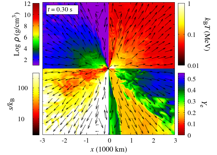
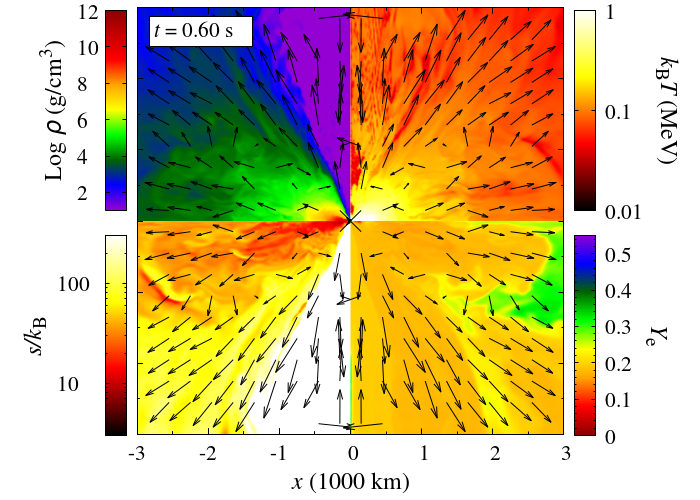
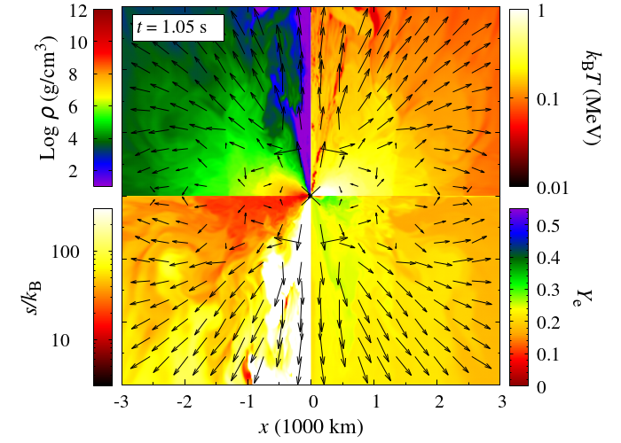
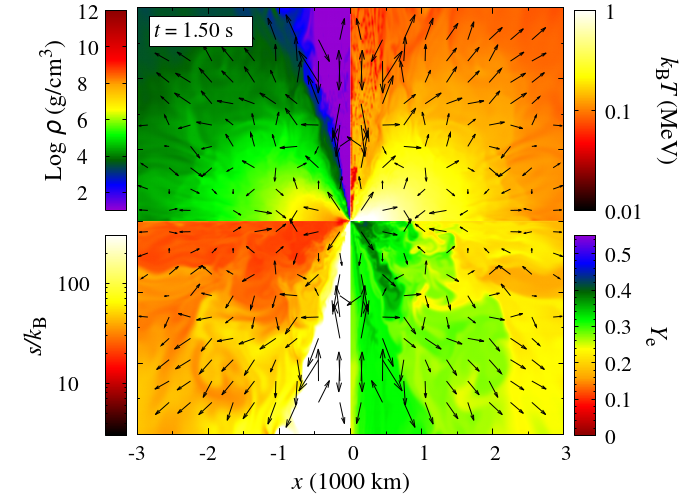
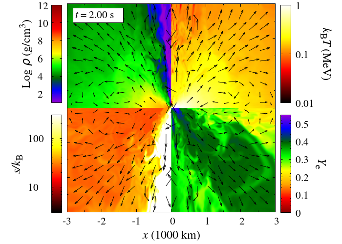
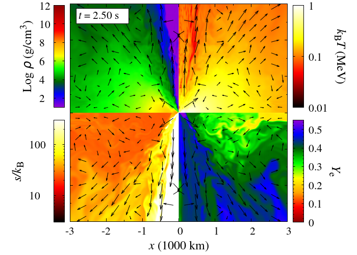
Figure 1: Snapshots of the rest-mass density in units of ${\rm g/cm}^{3}$, temperature ($k_{\rm B}T$ in units of MeV with $k_{\rm B}$ being the Boltzmann constant), specific entropy $s$ in units of $k_{\rm B}$, and electron fraction $Y_{e}$ at selected time slices for model M10L75a with the high-resolution run. The arrows denote the velocity field of $(v^{x},v^{z})$.

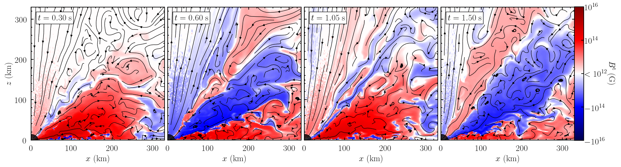
Figure 2: Evolution of the poloidal magnetic-field lines together with the toroidal magnetic-field strength (color profile) in the near zone of $|x|\leq 330$ km and $|z|\leq 330$ km for model M10L75a with the high-resolution run.

III.2.1 Evolution of the system

First, we briefly summarize the evolution process of the disk determined by the dynamo action described in Sec. II.2. By the $\alpha$-$\Omega$ dynamo effect, the poloidal magnetic field is developed from the purely toroidal field initially given. By the subsequent $\alpha$-$\Omega$ dynamo effect and the winding of the magnetic field lines of the generated poloidal field, the toroidal field is also enhanced. After the significant amplification of the magnetic-field strength, with which its fastest growing mode can be resolved, the MRI also plays an important role [37]. Because of the resulting development of the turbulent state in the disk, the disk matter expands and a part of it is ejected from the disk in a quasi-spherical manner: The major part is ejected primarily toward the non-polar direction because of the presence of the angular momentum barrier, but an outflow of the low-density matter is also observed in the polar direction (see Fig. 1 for model M10L75a). A funnel with the half opening angle of $10^{\circ}$–$15^{\circ}$ is typically formed around the $z$-axis after the outflow is steadily driven. The resultant funnel region has a high ratio of the magnetic pressure to the gas pressure (i.e., low-$\beta$ plasma). All these features are found irrespective of the values of $\sigma_{\rm c}$ and $\alpha_{\rm d}$ employed in the present work, and are qualitatively very similar to those found in viscous hydrodynamics simulations [29, 30]. However, the qualitative and quantitative details are different between the results of viscous hydrodynamics and MHD (see below). Also the MHD results depend quantitatively on the values of $\sigma_{\rm c}$ and $\alpha_{\rm d}$.

The matter outflow is accompanied by the ejection of the magnetic loops from the disk. This generates the large-scale poloidal and toroidal magnetic fields outside the disk. At the same time, in the disk, highly disturbed magnetic fields are developed reflecting its turbulent motion. Furthermore, in the presence of the dynamo, the polarity of the magnetic field is often changed. Figure 2 displays the poloidal magnetic field lines together with the toroidal magnetic-field strength for model M10L75a. Here, the red and blue colors denote that the toroidal field is positive and negative, respectively. This figure shows that highly distorted poloidal-magnetic fields are indeed developed in the accretion disks after the enhancement of the magnetic-field strength by the dynamo process reflecting the development of a turbulent motion inside the disk. Some of the field lines are extended outside the disk and form the global magnetic fields. It is also found that an aligned magnetic field is developed in the funnel region near the $z$-axis. All these features in the outcome are qualitatively the same as those often found in the ideal MHD simulations for the accretion disks around the black hole (e.g., Refs. [27, 38, 66, 67, 68, 69, 70, 71]), for which the ideal MHD simulations are for most cases started from a seed poloidal field and the turbulence is developed purely (in the first principle manner) by the MRI.

One interesting feature in the simulations with the mean-field dynamo term is that the magnetic-field polarity changes [50] in a quasi-periodic manner, with the period of several hundred ms in our present setting (see Sec. II.2). The color profile of Fig. 2 illustrates that the toroidal-field polarity indeed changes as found in the high-resolution three-dimensional ideal MHD simulation [27, 38]. Also, near the $z$-axis, the poloidal-field polarity changes in the same period as that for the toroidal field (see the arrows of the poloidal field lines in Fig. 2). This implies that an entirely coherent, aligned magnetic field is not established in the large scale, although coherent magnetic-field lines near the $z$-axis are locally developed, and that during the change of the polarity of the poloidal field near the $z$-axis, not an aligned magnetic field but a disturbed field configuration transiently appears.

In the late evolution stage in which the mass and density of the accretion disk decrease, the magnetic-field strength decreases. In particular in the very late stage in which the matter motion is dominated by the turbulent motion (not by a coherent rotational motion in the disk), the poloidal field near the $z$-axis does not have a very aligned structure (and as a result, the polar outflow ceases). All these features are found irrespective of the mean-field dynamo parameters employed.

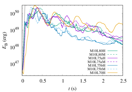
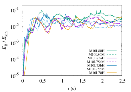
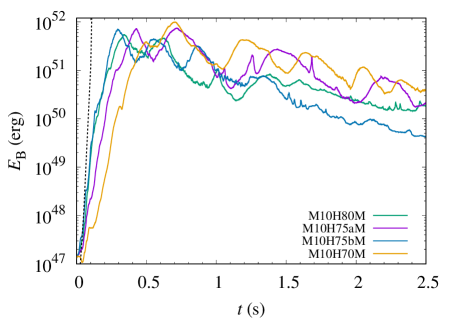
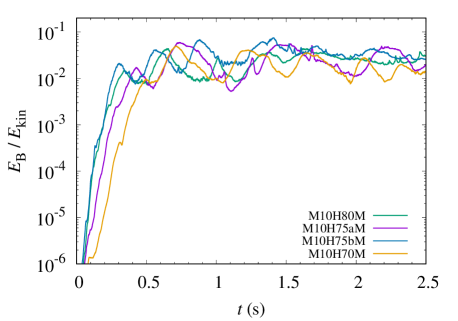
Figure 3: Upper panels: Evolution of the electromagnetic energy and ratio of the electromagnetic energy to the kinetic energy for the systems of a black hole and a low-mass disk listed in Table 1. Lower panels: The same as the upper panels but for the systems of a black hole and a high-mass disk listed in Table 1. The black dotted lines in the left two panels show $\propto\exp(2\omega_{\rm max}t)$ with $\alpha_{\rm d}=10^{-4}$, $\sigma_{\rm c}=10^{8}\,{\rm s}^{-1}$, and $|S_{\Omega}|=10^{3}\,{\rm rad/s}$: cf. Eq. (13).

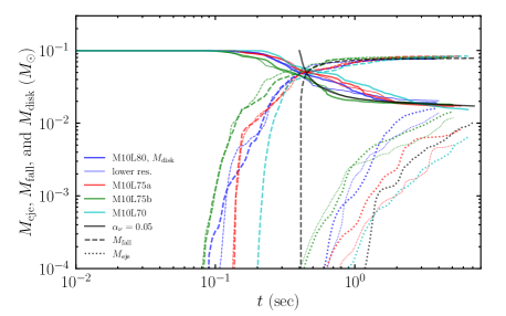
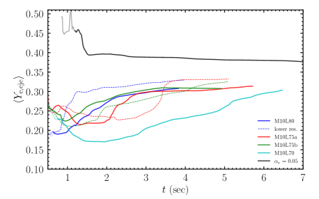
(a) (b)
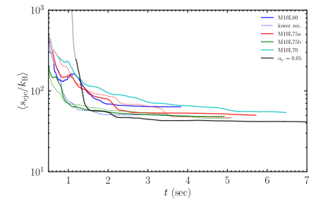
(c) (d)

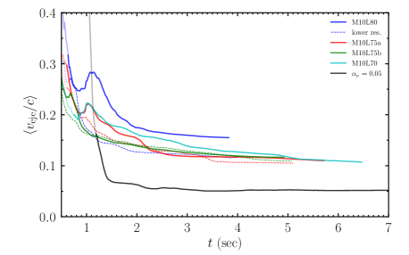
Figure 4: Evolution of several quantities for the low-mass disk surrounding a black hole. (a) Mass of the matter located outside the black hole (solid curves), that falls into the black hole (dashed curves), and ejected from the system (dashed curves). The thick and thin curves denote the results with the high- and medium-resolution runs, respectively. (b) the average entropy per baryon for the ejecta; (c) the average value of $Y_{e}$ for the ejecta; and (d) the average velocity for the ejecta. For (b)–(d), the solid and dashed curves denote the high- and medium-resolution results. For comparison, the results by a viscous hydrodynamics simulation performed in Ref. [30] are presented for all the panels with the time shift of $+0.4$ s.

Upper panels of Fig. 3 plot the evolution of the electromagnetic energy, $E_{\rm B}$, and the ratio of $E_{\rm B}$ to the kinetic energy, $E_{\rm kin}$, as functions of time for the systems of a black hole and a low-mass disk. For all the models, the electromagnetic energy increases exponentially with time in the early stage of the evolution. The growth timescale, indicated by the black dotted line in the left panels of Fig. 3, agrees approximately with the expression of Eq. (13): As this equation indicates, for the models with the higher values of $\sigma_{\rm c}$ and $\alpha_{\rm d}$, the growth timescale is shorter. It is also found that the curves of $E_{\rm B}$ oscillate with time. This is likely to be the reflection of the fact that there are multiple oscillatory modes in the presence of the dynamo term; during the change of polarity of the magnetic fields with multiple modes, the field strength should change in time (see the discussion in Sec. II.2).

After the early exponential increase of the electromagnetic energy, the growth rate becomes smaller due to the back reaction of the matter affected by the electromagnetic force. Associated with this reaction, the mass outflow sets in. Eventually, the exponential growth is stopped when the ratio of the electromagnetic energy to the kinetic energy, $E_{\rm B}/E_{\rm kin}$, reaches $\approx 0.03$–$0.1$. At this stage, the early-time mass ejection is most activated (see, e.g., Fig. 4). Subsequently, the ratio of $E_{\rm B}/E_{\rm kin}$ remains to be between $10^{-2}$ and $10^{-1}$ as often found in the accretion disks with an equipartition state. This ratio is slightly higher for the larger values of $\sigma_{\rm c}$ for this low-mass disk model. In the stage of the relaxed value of $E_{\rm B}/E_{\rm kin}$, due to the angular momentum transport associated with the MHD effect, a substantial fraction of the disk matter falls into the black hole, and the disk mass decreases with time (see Fig. 4). Note that the disk mass also decreases partly (in the present case $\sim 20\%$ of the initial disk mass) due to the mass ejection. Associated with the mass infall and mass ejection, the electromagnetic energy of the disk decreases with time, although the ratio, $E_{\rm B}/E_{\rm kin}$, is preserved to be of $O(0.01)$ (cf. Fig. 3). The decrease rate of $E_{\rm B}$ is smaller for smaller values of $\sigma_{\rm c}$ and $\alpha_{\rm d}$, because the mass infall and ejection proceed more slowly.

We note that the upper two panels of Fig. 3 indicate that the dependence of the electromagnetic-energy curve on the grid resolution is weak. Thus, the MHD evolution process of the disk is likely to be captured well with the current grid resolutions.

The lower panels of Fig. 3 display the evolution of $E_{\rm B}$ and $E_{\rm B}/E_{\rm kin}$ for the high-mass disk models. It is found that the evolution processes of these quantities are qualitatively similar to those for the low-mass disk models. The dependence of the ratio of $E_{\rm B}/E_{\rm kin}$ on $\sigma_{\rm c}$ is weaker than that for the low-mass model, and it varies in a narrow range approximately between 0.01 and 0.04. For both low-mass and high-mass disk models, the electromagnetic energy for the models with $\alpha_{\rm d}=2\times 10^{-4}$ is smallest for $t\gtrsim 1$ s among the models with the same disk mass. The reason for this is that the mass ejection proceeds earlier for the larger value of $\alpha_{\rm d}$ (cf. Figs. 4(a) and 6(a)). Thus the value of $\alpha_{\rm d}$ controls the mass ejection timescale for the black hole-disk system.

III.2.2 Mass ejection

Figure 4(a) shows the evolution of the disk mass, the rest mass that falls into the black hole, and ejecta mass. For comparison, numerical results derived by our viscous hydrodynamics simulation [30] are presented together. Since the mass ejection is delayed by the growth timescale of the turbulent state in the present MHD simulations, we shift the results for the viscous hydrodynamics simulation by $+0.4$ s in time. The evolution curves of the mass outside the black hole indicate that, as in our viscous hydrodynamics simulation, about 20% of the initial disk mass is likely to be ejected from the system and the rest of the matter falls into the black hole for all the models. These fractions are in a good agreement with those in viscous hydrodynamics. For models M10L75a and M10L70, the mass ejection timescale is longer than the simulation time, and thus, the ejecta mass does not settle to the final value in $\sim 6$ s. However the curves for the ejecta mass and disk mass are similar to those in other MHD models, and hence, we may expect that the ejecta mass will approach asymptotically $\sim 0.02M_{\odot}$.

The mass ejection timescale in the MHD simulations is shorter for the larger values of $\sigma_{\rm c}$ and $\alpha_{\rm d}$ (see the curves for models M10L80 and M10L75b in Fig. 4(a)). This is natural because for the larger values of these two parameters, the growth timescale of the magnetic-field strength is shorter (cf. Sec. II.2). In addition, the $\alpha$-$\Omega$ dynamo instability occurs for the shorter-wavelength modes with the larger values of these parameters (cf. Eq. (12)), resulting in the higher magnetic power and earlier mass ejection. Although this timescale depends on the choice of the parameters as in the case of viscous hydrodynamics in which the mass ejection timescale depends on the viscous coefficient, the timescale is universally seconds in the reasonable choice of the parameters. It should be also mentioned that the numerical results depend only weakly on the grid resolution, although with the higher grid resolution, the mass ejection sets in earlier perhaps due to the better-resolved magnetic-field growth (for the dynamo instability as well as for the MRI).

Figure 4(b)–(d) plot the evolution of the average values of the specific entropy, electron fraction, and velocity for the ejecta. Again, for comparison, we plot the results in our viscous hydrodynamics [30] together with the time shift of $+0.4$ s. It is found that all the quantities take similar but slightly different asymptotic values from those obtained in the viscous hydrodynamics simulations irrespective of the values of $\sigma_{\rm c}$ and $\alpha_{\rm d}$. Slightly systematic differences are found as follows: (i) The asymptotic value of the average electron fraction of the ejecta in the MHD simulations is by $\sim 0.05$ smaller than that in viscous hydrodynamics; (ii) The average velocity of the ejecta in the MHD simulations is $\sim 0.1c$–$0.15c$, while it is $\sim 0.05c$ in viscous hydrodynamics (the average velocity becomes high only for $\sigma_{\rm c}=10^{8}\,{\rm s}^{-1}$, but for others, it is universally $\approx 0.1c$). The second fact (ii) is in particular likely to be related to the difference in the mechanisms of the mass ejection between MHD and viscous hydrodynamics. Thus, in the following, we discuss our interpretation for this difference in the mass ejection mechanism in more detail.

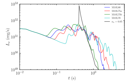
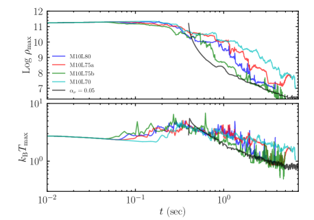
Figure 5: Upper panel: Evolution of the neutrino luminosity for the low-mass disk model. Lower panel: Evolution of the maximum rest-mass density in units of ${\rm g/cm}^{3}$ and maximum temperature ($k_{\rm B}T_{\rm max}$) in units of MeV. For comparison, the results by a viscous hydrodynamics simulation performed in Ref. [30] are presented with the time shift of $+0.4$ s.

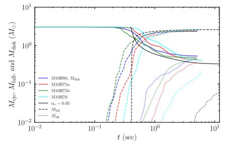
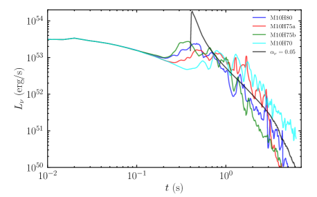
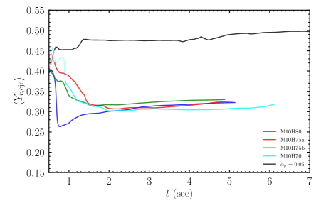
(a) (b) (c) (d)

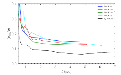
Figure 6: Evolution of several quantities for the high-mass disk surrounding a black hole. (a) Mass of the matter located outside the black hole (solid curve), that falls into the black hole (dashed curve), and ejected from the system (dashed curve); (b) neutrino luminosity; (c) the average value of $Y_{e}$ for the ejecta; (d) the average velocity of the ejecta. For comparison, the results by a viscous hydrodynamics simulation performed in Ref. [30] are presented with a time shift of $+0.4$ s for all the panels.

For the case of viscous hydrodynamics, the mass ejection is driven by the viscous heating after the disk is substantially evolved by the viscous angular momentum transport by which the density and temperature of the disk are decreased so significantly that the neutrino cooling becomes inefficient [18, 29]. Here, it is worth mentioning that in viscous hydrodynamics, the viscous heating is the only channel for the mass ejection, and only when the thermal energy gained by this heating is not significantly dissipated by some other cooling processes such as the neutrino cooling, the mass ejection can occur. In MHD, on the other hand, the situation is different: In this case, the turbulence induced by the MHD instability enhances an effective viscosity and drives the angular momentum transport and (effective) viscous heating in the same manner as in viscous hydrodynamics, but there are additional magnetic-field effects associated with the global motion of the magnetic-field lines. In particular, in the presence of differential rotation, the magneto-centrifugal [72] and magnetic-tower (e.g., Ref. [73]) effects can play an important role in the mass ejection. By these effects, the mass ejection can be driven even in the absence of the effective viscous heating. In addition, the ejecta as well as the matter in the outer region can be accelerated outward by the magnetic power, even in the presence of an efficient cooling process.

This interpretation is supported by observing the neutrino luminosity as a function of time; see the upper panel of Fig. 5. In this figure, we compare the neutrino luminosity in the MHD simulations with the viscous hydrodynamics one. Note that for the result of viscous hydrodynamics (black solid curve), the time is shifted by $+0.4$ s. As shown in Ref. [29], in viscous hydrodynamics, the mass ejection sets in when the neutrino cooling rate is much smaller than the viscous heating rate; i.e., $L_{\nu}$ decreases below $\sim 10^{50}$ erg/s. On the other hand, in MHD, the mass ejection is activated even in the stage with $L_{\nu}\sim 10^{51}$ erg/s (see Fig. 4(a) and Fig. 5). This is in particular the case for models M10L75b and M10L80. This early-time mass ejection is likely to be driven primarily by the pure MHD effects. For all the models, however, the mass ejection is also active for the stage of low neutrino luminosity. This late-time mass ejection is likely to stem primarily from the effective viscous effect associated with the enhanced turbulent viscosity and inefficient neutrino cooling. That is, there are multiple channels for the mass ejection in MHD [27, 35].

It is also found that the peak neutrino luminosity in MHD is at most $10^{52}$ erg/s while it is $\sim 10^{53}$ erg/s in viscous hydrodynamics. This indicates that the heating in MHD is not enhanced as efficiently as in viscous hydrodynamics, as the neutrino emission is closely related to the thermal energy of the matter. On the other hand, the high-luminosity stage with $L_{\nu}\sim 10^{51}$ erg/s continues for a long timescale of $\sim 1$ s in MHD while the stage with $L_{\nu}\gtrsim 10^{51}$ erg/s is only for $\sim 300$ ms in viscous hydrodynamics. This indicates that the instantaneous heating efficiency in MHD is not as high as that in viscous hydrodynamics but the heating is continued constantly for a long timescale. In other words, the timescale of the disk expansion resulting from the (turbulent) viscous or MHD effect is not as short as in viscous hydrodynamics. This fact is found from the evolution of the maximum rest-mass density of the disk (see the bottom panel of Fig. 5): In the MHD simulations, the high value of the maximum rest-mass density is preserved for a longer timescale than in the viscous hydrodynamics simulation. This is also reflected in the fact that the maximum temperature in MHD is higher than that in viscous hydrodynamics for $t\gtrsim 1$ s. We here note that for model M10L80, the curves of $L_{\nu}$, $\rho_{\rm max}$, and $T_{\rm max}$ in the late time are similar to those for the viscous hydrodynamics model, but this is accidental: For model M10L80, the disk expansion and mass ejection are driven mainly by the MHD effect with a short timescale.

For the high-mass disk case, the difference in the mechanism for the mass ejection between MHD and viscous hydrodynamics becomes even more remarkable. Figure 6(a) shows the evolution of the disk mass, the rest mass that falls into the black hole, and ejecta mass. For comparison, again, numerical results derived by our viscous hydrodynamics simulation with plausible viscous parameters [30] are also presented. It is found that irrespective of the values of $\sigma_{\rm c}$ and $\alpha_{\rm d}$ the asymptotic values of the mass for the matter located outside the horizon in the MHD simulations are larger than that in the viscous hydrodynamics one (and thus the mass that falls into the black hole in the MHD simulations are smaller than that in viscous hydrodynamics). In addition, the onset time of the mass ejection in the MHD simulation is substantially earlier than that in the viscous hydrodynamics one. As we already mentioned, in viscous hydrodynamics, the mass ejection sets in only after the neutrino cooling becomes inefficient. For the high-mass disk model, the neutrino luminosity is preserved to be high for a long timescale of several seconds in both MHD and viscous hydrodynamics (see Fig. 6(b)). In viscous hydrodynamics, this makes the onset time of the mass ejection later than that in the low-mass disk model [30]. On the other hand, in MHD, the difference in the onset time of the mass ejection is not appreciable between the high-mass and low-mass disk models. This indicates that the MHD effects, not viscous effects, play a primary role in the mass ejection. In particular, for the high-mass disk case for which the pressure of the disk is larger than that in the low-mass disk case, the magnetic-field strength is enhanced to a higher level in an equipartition stage (cf. Fig. 3), and furthermore, the high-density region of the disk, which is located in its deep inside, can play a role of an anchor for sustaining and swinging the field lines of strong magnetic fields, leading to the increase of the mass ejection efficiency via the magneto-centrifugal effect [72]. This indicates that, in the presence of a high-mass dense object in the central region, the efficiency of the mass ejection is enhanced. This effect is in particular important in the presence of a neutron star at the center (see Sec. IV).

Figure 6(c) and (d) plot the evolution of the average electron fraction and velocity of the ejecta as in Fig. 4. In comparison with the viscous hydrodynamics results, a significant difference is again found in the asymptotic values of the average velocity: The average ejecta velocity in the MHD simulations is by a factor of $\sim 2$ larger than the viscous hydrodynamics results in the chosen ranges of $\sigma_{\rm c}$ and $\alpha_{\rm d}$ (in this case the dependence of the ejecta velocity on $\sigma_{\rm c}$ is weak). This is likely due to the enhanced MHD effects, in particular to the magneto-centrifugal effect [72], as mentioned above. An appreciable difference between the MHD and viscous hydrodynamics results is also found in the average electron fraction. For the MHD simulations, the average value of the electron fraction settles to $\sim 0.35$ irrespective of the values of $\sigma_{\rm c}$ and $\alpha_{\rm d}$, while in the viscous hydrodynamics simulation, it is $\sim 0.5$. The reason for this high value in viscous hydrodynamics is that for the high-mass disk model, the timescale of the mass ejection from the disk is quite long, about several seconds, and during the long-term evolution process of the disk, the density becomes low enough to decrease the electron degeneracy while keeping relatively high temperature, and as a result, the electron fraction is increased via the weak interaction process [30]. By contrast, in the MHD simulations, the mass ejection is not primarily driven by the effective viscous process resulting from the turbulent viscosity developed, but mainly by the MHD activity such as magneto-centrifugal force, which significantly shortens the mass ejection timescale (see Fig. 6(a)). As a result of these effects, the electron fraction of the ejecta remains to be fairly low preserving the low values of the high-density state of the disk.

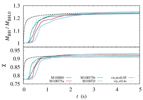
Figure 7: The evolution of the mass and dimensionless spin of black holes for the high-mass disk model. The dashed curves are the results by a viscous hydrodynamics simulation performed in Ref. [30] (for the original result and for the results with the time shift of $+0.4$ s). In the upper panel, the black-hole mass in units of its initial mass is plotted.

III.2.3 Evolution of black hole

Although the mass ejection mechanism is different between the MHD and viscous hydrodynamics models, the evolution process of the black hole as a result of the mass accretion is similar in both approaches. Figure 7 shows the evolution of the mass and dimensionless spin of the black hole for all the high-mass disk models. For comparison, we also plot the results obtained by the viscous hydrodynamics simulation [30]. Irrespective of the MHD or viscous hydrodynamics, the dimensionless spin increases with the mass infall into the black hole and settles eventually to a saturated value of $\approx 0.92\pm 0.01$ at $t\sim 3$ s. Although the mass accretion still continues for $t>3$ s and the black-hole mass gradually increases, the dimensionless spin does not increase significantly. This result suggests the similarity of the angular momentum transport by the MHD and viscous processes. The evolution curves of the black-hole mass by the MHD simulations are also similar to that by the viscous hydrodynamics simulation with a reasonable viscous coefficient. The black-hole mass in the MHD simulations is slightly smaller than that in the viscous hydrodynamics simulation. The reason for this is that the fraction of the ejecta mass in the MHD simulation is slightly larger than in the viscous hydrodynamics simulations due to the MHD effects.

We note that for larger values of $\sigma_{\rm c}$ and $\alpha_{\rm d}$, the relaxed values of the dimensionless spin is slightly smaller and the black-hole mass is slightly smaller. This reflects the fact that the outward angular-momentum transport effect and resulting mass ejection are more efficient for the larger values of $\sigma_{\rm c}$ and $\alpha_{\rm d}$.

IV Evolution of a remnant of binary neutron star merger

IV.1 Setup

Table 2: Initial conditions and setup for the numerical simulations of a binary neutron star merger remnant. For all the initial conditions, the total baryon mass is $M_{*}=2.95M_{\odot}$, the gravitational mass is $M=2.64M_{\odot}$, the total rotational kinetic energy is $E_{\rm kin}\approx 1.16\times 10^{53}$ erg, the electromagnetic energy is $E_{\rm B}\approx 2.61\times 10^{47}$ erg, and the total angular momentum is $J=4.65\times 10^{49}$ g cm²/s.

Model	$\sigma_{\rm c}\,{\rm(s^{-1})}$	$\alpha_{\rm d}$	$\Delta x_{0}$ (m)
MNS80	$1\times 10^{8}$	$1\times 10^{-4}$	160, 200
MNS75a	$3\times 10^{7}$	$1\times 10^{-4}$	160, 200
MNS75b	$3\times 10^{7}$	$2\times 10^{-4}$	160
MNS75c	$3\times 10^{7}$	$5\times 10^{-5}$	160
MNS70a	$1\times 10^{7}$	$1\times 10^{-4}$	160
MNS70b	$1\times 10^{7}$	$2\times 10^{-4}$	160

We then turn our attention to the evolution of a binary-neutron-star merger remnant, which is composed of a massive neutron star and a torus. As in our series of the papers [23, 24, 31, 34], the initial condition for the matter field is supplied from the result of a simulation for the binary neutron star merger. Specifically, we employ the DD2-135 model of Ref. [31]: a merger remnant of binary neutron stars with each neutron-star mass $1.35M_{\odot}$. This model was already evolved in viscous hydrodynamics with the (viscous) $\alpha$-parameter of 0.04 and the scale height of 10 km in a previous paper [31]. We compare the results obtained in the present GRRRMHD simulations with those in the viscous hydrodynamics ones for several choice of $\sigma_{\rm c}$ and $\alpha_{\rm d}$ in the following.

Again, we initially superimpose a purely toroidal magnetic field in a high-density region of the remnant (both neutron star and torus) as

$${\cal{B}}^{T}=\varpi{\cal{B}}^{\varphi}=A_{0}\varpi z\,{\rm max}\left({P\over P_{\rm max}}-0.01,0\right).$$ (33)

The poloidal component of ${\cal{B}}^{i}$ is set to be zero and the electric field is determined by the ideal MHD condition of ${\cal{E}}^{i}=-\epsilon^{ijk}u_{j}{\cal{B}}_{k}/w$. The dependence on the coordinates, $\varpi z$, in Eq. (33) stems from the regularity condition along the $z$-axis and the reflection anti-symmetry with respect to the $z=0$ plane for ${\cal{B}}^{T}$. $A_{0}$ is a constant, and in this work, we choose it so that the electromagnetic energy is $E_{\rm B}\approx 2.6\times 10^{47}$ erg. We note again that the numerical results depend very weakly on the initial field strength because the electromagnetic field grows exponentially with time in the early stage until a universal saturation level of the field strength is reached. With the setting of Eq. (33), the magnetic fields are initially present in the massive neutron star and in the high-density region of the torus. As already mentioned in Sec. III, the magnetic-field growth is driven purely by the dynamo instability for the initial condition only with the toroidal magnetic field in the axisymmetric simulation.

For the numerical simulation, the central region with $x\lesssim 30$ km and $z\lesssim 30$ km is covered by the uniform grid of $\Delta x_{0}=\Delta z_{0}=160$ m or $200$ m and outside this region, the grid spacing is increased as $\Delta x_{i+1}=1.0075\Delta x_{i}$ and $\Delta z_{j+1}=1.0075\Delta z_{j}$. We basically perform the simulations with the higher grid resolution of $\Delta x_{0}=\Delta z_{0}=160$ m, but to confirm the weak dependence of the results on the grid resolution, for selected models (MNS75a and MNS80), we also perform the simulations with $\Delta x_{0}=\Delta z_{0}=200$ m. The models employed in this paper are listed in Table 2. Unless otherwise stated, the results with the higher-resolution setting are presented in the following. For all the models, the initial value of the kinetic energy is $E_{\rm kin}\approx 1.16\times 10^{53}$ erg.

IV.2 Numerical results

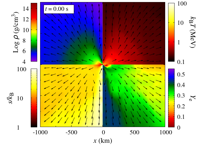
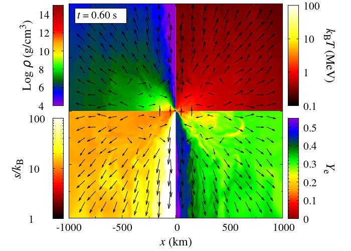
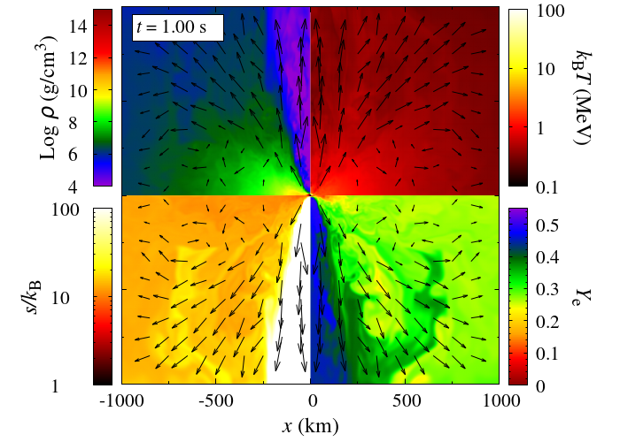
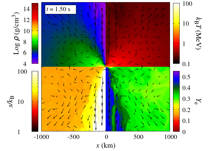
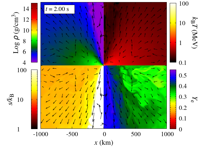
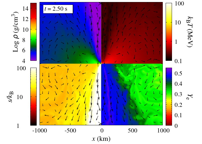
Figure 8: Snapshots of the rest-mass density in units of ${\rm g/cm}^{3}$, temperature ($k_{\rm B}T$ in units of MeV), specific entropy $s$ in units of $k_{\rm B}$, and electron fraction $Y_{e}$ at selected time slices for model MNS75a with the high-resolution run. The arrows denote the velocity field of $(v^{x},v^{z})$.

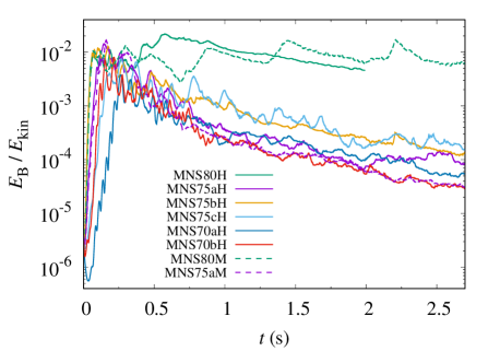
Figure 9: Evolution of the electromagnetic energy (left) and ratio of the electromagnetic energy to the kinetic energy (right) for all the models listed in Table 2. The solid and dashed curves show the results with the high- and medium-resolution runs, respectively. The dotted black line in the left panel shows $\propto\exp(2\omega_{\rm max}t)$ with $\alpha_{\rm d}=10^{-4}$, $\sigma_{\rm c}=10^{8}\,{\rm s}^{-1}$, and $|S_{\Omega}|=10^{3}\,{\rm rad/s}$: cf. Eq. (13).

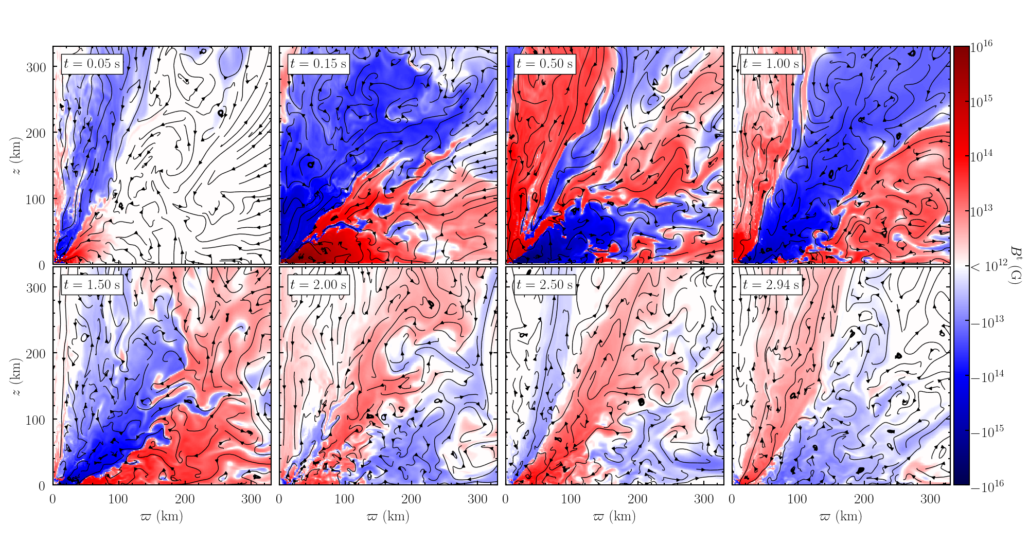
Figure 10: The poloidal magnetic-field lines together with the toroidal magnetic-field strength (color profiles) at selected time slices for model MNS75a.

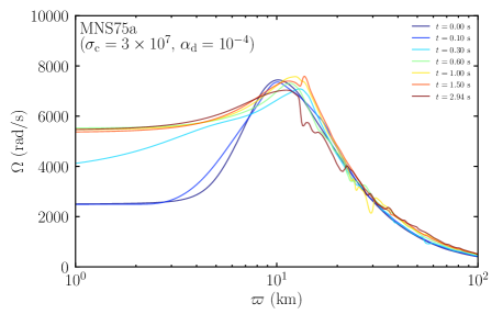
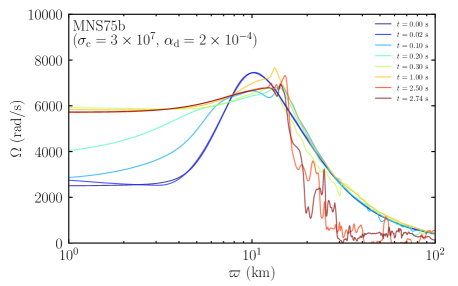
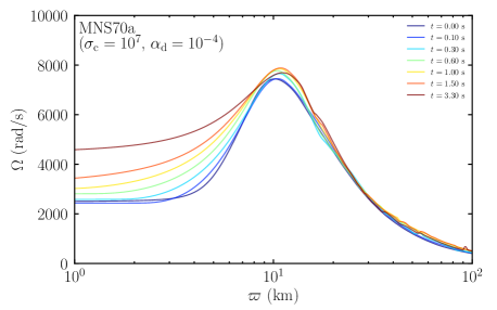
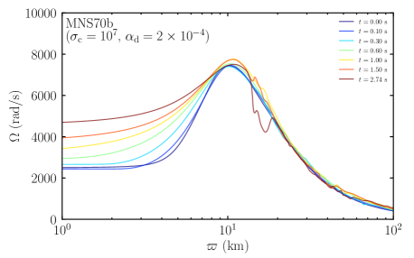
Figure 11: Evolution of the angular velocity as a function of $\varpi$ with $z=1$ km for models MNS75a (top left), MNS75b (top right), MNS70a (bottom left), and MNS70b (bottom right). Note that for model MNS75b, the quasi-steady-state disk is absent for $t\gtrsim 2$ s because most of the disk matter is ejected by the magneto-centrifugal effect.

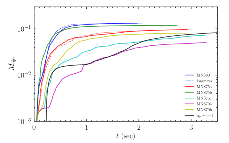
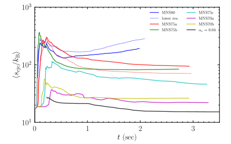
(a)   (b)
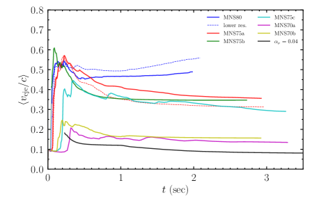
(c)   (d)

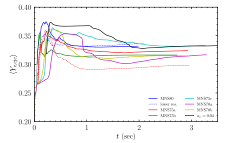
Figure 12: Evolution of (a) rest mass, (b) average velocity, (c) average specific entropy, and (d) average electron fraction of the ejecta for all the models listed in Table 2. The solid and dashed curves show the results with the high- and medium-resolution runs, respectively. For comparison, the results for a viscous hydrodynamics simulation (model DD2-135M in Ref. [31]) are plotted together with the time shift of $+0.2$ s.

First of all, we display Fig. 8, which shows the evolution of the rest-mass density, the temperature, the specific entropy, and the electron fraction for $\sigma_{\rm c}=3\times 10^{7}\,{\rm s}^{-1}$ and $\alpha_{\rm d}=10^{-4}$ (model MNS75a). This illustrates a typical evolution feature of the torus surrounding a neutron star in the present MHD simulations: Due to the angular momentum transport and heating associated with the MHD process caused by the enhanced magnetic fields resulting from the dynamo action, the torus gradually expands and the matter is ejected from the system spending $\sim 1$ s. Eventually, the rest-mass density of the torus becomes much lower than the initial value, and thus, the final outcome is a massive neutron star with a low-density torus and its envelope. During the evolution, it is also found that a funnel region with the half opening angle of $10^{\circ}$–$15^{\circ}$ is established along the $z$-axis. In the funnel region, the electromagnetic pressure is comparable to or larger than the gas pressure (i.e., with the plasma-$\beta$ of $\lesssim 1$). The resultant density profile is very similar to those in viscous hydrodynamics (compare Fig. 8 with Fig. 1 of Ref. [31]). However, the mechanisms of the angular momentum transport and heating in the torus and the mass ejection process are quite different from those in viscous hydrodynamics. In particular, the unique properties of the MHD processes can enhance the efficiency of the mass ejection in the presence of strong magnetic fields that have a base point (anchor) in the massive neutron star. In the following, we pay particular attention to such unique properties resulting from the MHD process.

Figure 9 shows the evolution of the electromagnetic energy (left) and the ratio of the electromagnetic energy to the kinetic energy ($E_{\rm B}/E_{\rm kin}$: right), respectively, for the entire system of the remnant massive neutron star and the torus surrounding it. As in the evolution for black-hole accretion disks, the magnetic-field strength is initially amplified in the exponential manner until $E_{\rm B}/E_{\rm kin}$ reaches $\sim 3\times 10^{-3}$–$1\times 10^{-2}$, and then the amplification is saturated irrespective of the values of $\sigma_{\rm c}$ and $\alpha_{\rm d}$. Here we note that the kinetic energy, $E_{\rm kin}$, is dominated by that of the neutron star. The typical maximum magnetic-field strength is $\sim 10^{16}$ G as found in Ref. [34] (also comparable to that in the remnant of binary neutron star mergers at a few ms after the merger [74]). Here the saturation occurs due to the fact that after the quick magnetic-field amplification, the matter and magnetic flux start being ejected from the neutron star and inner part of the torus primarily toward the polar direction like in the magnetic-tower outflow (see Fig. 10; see also Ref. [34]), and the further amplification is suppressed. These initial mass and magnetic-flux ejections occur approximately when the maximum electromagnetic energy is reached, i.e., at $\sim 0.2$–0.3 s after the start of the simulation. This initial ejection is stronger for the larger values of $\sigma_{\rm c}$ and $\alpha_{\rm d}$ because of the rapid growth of the magnetic-field strength by the dynamo effect. In particular, for the cases of $\sigma_{\rm c}=10^{8}\,{\rm s}^{-1}$ and of $\sigma_{\rm c}=3\times 10^{7}\,{\rm s}^{-1}$ and $\alpha_{\rm d}=2\times 10^{-4}$ (models MNS80 and MNS75b, respectively), this early mass ejection explosively occurs and becomes the dominant mass ejection process among the entire evolution.

After the initial ejection toward the polar region, the magnetic fields also spread to the equatorial region because of the strong magnetic pressure and magneto-centrifugal effect. Then, the matter and magnetic-field flux start being outflowed toward a variety of the directions and a global magnetic-field profile is established. After the initial violent ejection, matter outflow quasi-steadily continues. As we already mentioned, this early ejection is in particular strong for models MNS80 and MNS75b. For these models, the torus around the massive neutron star is significantly disturbed during the formation of the magnetic-field tower structure.

Because the poloidal magnetic field is developed by the $\alpha$-$\Omega$ dynamo and associated outflow, the magnetic braking is subsequently activated in the neutron star, and then, the degree of the differential rotation in the neutron star becomes weak: inside it, the angular velocity profile approaches a rigid state in particular for models with $\sigma_{\rm c}\geq 3\times 10^{7}\,{\rm s}^{-1}$ (see Fig. 11). As a consequence, the value of $|S_{\Omega}|$ in the inner region of the neutron star becomes small, leading to the suppression of the $\alpha$-$\Omega$ dynamo there. However, the differential rotation is still present in the outer part of the neutron star and torus. Hence, the $\alpha$-$\Omega$ dynamo is still active in the outer part of the system, preserves the turbulent state of the torus, and induces the resulting mass ejection from the torus. We note that the amplification of the magnetic field initially occurs both in the neutron star and torus, but the total electromagnetic energy is initially determined by that in the neutron star. Also, the kinetic energy is always dominated by that of the neutrons star and does not change significantly. For these reasons, the shapes of the curves of $E_{\rm B}$ and $E_{\rm B}/E_{\rm kin}$ are similar to each other.

The evolution of the electromagnetic energy inside the neutron star after the saturation of its growth depends strongly on the choice of $\sigma_{\rm c}$, which determines the dissipation timescale (for $S_{\Omega}=0$) given by

$$\tau_{\rm dis} \approx \left[{(kc)^{2}\over 4\pi\sigma_{\rm c}}-\alpha_{\rm d}kc\right]^{-1}$$ (34)

$$\approx 0.1\lambda_{20}\alpha_{{\rm d},-4}^{-1}\left(0.75\lambda_{20}^{-1}\alpha_{{\rm d},-4}^{-1}\sigma_{{\rm c},8}^{-1}-1\right)^{-1}\,{\rm s},~{}~{}$$

where $\lambda:=2\pi/k$, $\lambda_{20}:=\lambda/(20\,{\rm km})$, $\alpha_{{\rm d},-4}:=\alpha_{\rm d}/10^{-4}$, and $\sigma_{{\rm c},8}:=\sigma_{\rm c}/10^{8}\,{\rm s}^{-1}$, respectively. Note that if $\tau_{\rm dis}$ is negative, the system is unstable for the $\alpha$-dynamo with the corresponding wavelength. Thus, for $\sigma_{\rm c}=10^{8}\,{\rm s}^{-1}$ and $\alpha_{\rm d}=10^{-4}$, the electromagnetic field in the neutron star can be preserved by the unstable modes with $\lambda\gtrsim 15$ km, which is comparable to the neutron-star radius, while for the smaller values of $\sigma_{\rm c}\leq 3\times 10^{7}\,{\rm s}^{-1}$ (and $\alpha_{\rm d}\leq 2\times 10^{-4}$), the electromagnetic energy in the neutron star should be dissipated in $\sim 0.1$ s, because the modes with $\lambda\lesssim 45$ km decay.

Figure 9 indeed shows that for $\sigma_{\rm c}=10^{8}\,{\rm s}^{-1}$ (model MNS80), the electromagnetic energy is preserved after the saturation of the field growth. On the other hand, for $\sigma_{\rm c}\leq 3\times 10^{7}\,{\rm s}^{-1}$, the electromagnetic energy decreases with time and its magnitude depends weakly on the values of $\sigma_{\rm c}$ and $\alpha_{\rm d}$. The reason for this is that in this later stage, the electromagnetic energy is dominated by that of the torus in which the $\alpha$-$\Omega$ dynamo continues to be active. Indeed the magnitude of the electromagnetic energy, $10^{48}$–$10^{49}\,{\rm erg}$, is in broad agreement with the black hole-low-mass disk cases for which the order of the disk mass is the same as that for the torus surrounding the neutron star (compare the left panel of Fig. 9 with the top-left panel of Fig. 3). Figure 10 also shows that (i) as in the disk around the black hole (compare with Fig. 2), the polarity of the magnetic fields changes with time due to the dynamo effect and (ii) due to the dissipation of the magnetic field in the neutron star, the magnetic-field strength decreases along the $z$–axis in the late stage of $t\gtrsim 2$ s. These results are essentially the same as those in the black hole-disk case. On the other hand, we do not find clearly aligned structure for the magnetic-field lines in the funnel region. Our interpretation for this is that the matter outflow from the central region toward the polar region continuously occurs and the magnetic-field structure is always disturbed in the presence of the neutron star.

For $\sigma_{\rm c}=10^{7}\,{\rm s}^{-1}$ (models MNS70a and MNS70b), the dissipation timescale of the magnetic fields in the neutron star is so short that the magnetic braking effect is not very outstanding as found in the bottom panels of Fig. 11. That is, before the sufficient growth of the poloidal fields in the neutron star which activates the magnetic braking, the resistive effect becomes important, and hence, the differential rotation is preserved for a relatively long timescale. For these models, the effect of the neutron star on the mass ejection becomes relatively minor (see below).

Associated with the magnetic-field amplification, the matter is ejected from the merger remnant, primarily from the torus surrounding the massive neutron star. However, this does not imply that the role of the massive neutron star is not important for the mass ejection as described in the following.

As already mentioned, by the enhancement of the magnetic-field strength, the turbulent state is developed in the torus and the enhanced magnetic-field force induces the mass ejection from the torus (see, e.g., Figs. 8 and 10). This situation is qualitatively the same as that in the mass ejection from the black hole-disk systems. However, in the presence of the neutron star in the central region, the magneto-centrifugal effect [72] further enhances the mass ejection efficiency because some of the magnetic-field lines are anchored by the neutron star and the angular velocity of the neutron star is higher than that of the torus. Because of the presence of this additional effect, the total ejecta mass can be higher than that in the viscous hydrodynamics simulation with reasonable viscous parameters [31], in particular for the high values of $\sigma_{\rm c}$ (see Fig. 12(a)) with which the dissipation timescale of the magnetic fields in the neutron star is longer. In addition, the ejecta velocity is enhanced significantly for $\sigma_{\rm c}\geq 3\times 10^{7}\,{\rm s}^{-1}$ (see Fig. 12(b)). In particular for $\sigma_{\rm c}=10^{8}\,{\rm s}^{-1}$ (model MNS80), the average ejecta velocity becomes $\sim 0.5c$. Even for $\sigma_{\rm c}=3\times 10^{7}\,{\rm s}^{-1}$, the ejecta velocity is always by a factor of $\sim 2$ higher than that in viscous hydrodynamics, and the kinetic energy of the ejecta $\approx M_{\rm eje}v^{2}_{\rm eje}/2$ becomes $\gtrsim 10^{52}$ erg for models MNS80, MNS75a, MNS75b, and MNS75c. This implies that if the strong magnetic-field lines anchored in the neutron star are present for a few hundreds ms, the magneto-centrifugal force plays a significant role in the mass ejection. By contrast, if the strong magnetic field is present only for $\lesssim 100$ ms (i.e., $\sigma_{\rm c}\leq 10^{7}\,{\rm s}^{-1}$), the magneto-centrifugal force is likely to be a minor effect. In particular, if the dynamo effect is not strong, i.e., for MNS70a, the mass ejection efficiency in the MHD simulation is weaker than in the viscous hydrodynamics case. However, if the magnetic-field growth occurs in a short timescale, i.e., within $\sim 200$ ms, the strong magnetic-field effect is universally observed irrespective of the values of $\alpha_{\rm d}$ (compare the results for models MNS75a, MNS75b, and MNS75c).

The ejecta of kinetic energy, $E_{\rm kin,eje}$, gained primarily by the magneto-centrifugal force associated with the rotation of the neutron star, should also obtain the angular momentum approximately by $J_{\rm eje}\sim E_{\rm kin,eje}/\Omega$ where $\Omega$ is the relaxed angular velocity of the neutron star which is $\Omega\approx 6000$ rad/s (see Fig. 11). With this process, the neutron star should lose its angular momentum approximately by $J_{\rm eje}$. For $E_{\rm kin,eje}=10^{52}$ erg, $J_{\rm eje}\sim 3\times 10^{48}$ erg s. The angular momentum of the neutron star is approximately $3\times 10^{49}$ erg s. Thus, $\gtrsim 10\%$ of the angular momentum of the neutron star is transported to the ejecta for models with $\sigma_{\rm c}\geq 3\times 10^{7}\,{\rm s}^{-1}$. This result is reflected in the late-time decrease of the peak angular velocity for models MNS75a and MNS75b (see the upper panels of Fig. 11).

With the higher value of $\alpha_{\rm d}$, the magnetic field is amplified in a shorter timescale. As a result, the mass ejection sets in earlier (compare the results of Fig. 12(a) among models MNS75a, MNS75b, and MNS75c and/or between models MNS70a and MNS70b). However, the average velocity of the ejecta depends only weakly on the value of $\alpha_{\rm d}$. This indicates that the acceleration of the ejecta is induced primarily by the magneto-centrifugal force related to the amplified magnetic-field lines anchored in the neutron star.

Due to the violent magnetic-field activity and resulting shock heating, the specific entropy of the ejecta is also significantly enhanced, in particular for $\sigma_{\rm c}\geq 3\times 10^{7}\,{\rm s}^{-1}$ (see Fig. 12(c)). This results from the efficient shock heating by the MHD effect. By contrast, the average electron fraction is $\sim 0.3$, i.e., as high as that in the viscous hydrodynamics simulation, irrespective of the values of $\sigma_{\rm c}$ and $\alpha_{\rm d}$ (see Fig. 12(d)). One reason for this is that the majority of the matter is ejected from the outer part of the torus for which the density is not so high that the electron degeneracy is not very high, and thus, the neutron richness is only moderately high. The other reason is the presence of the strong irradiation by neutrinos emitted from the massive neutron star. Figure 13 plots the total neutrino luminosity as a function of time. It is found that the neutrino luminosity in the MHD simulations, $\sim 10^{53}\,{\rm erg/s}$, is only slightly smaller than that in viscous hydrodynamics. Thus, the neutrino irradiation in MHD can play a role as important as in viscous viscous hydrodynamics for controlling the electron fraction of the matter surrounding the neutron star and those ejected from it [31].

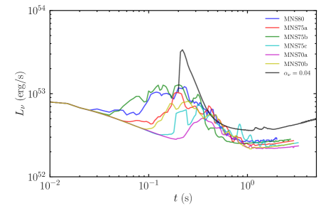
Figure 13: Evolution of the neutrino luminosity for all the high-resolution models listed in Table 2. For comparison, the result by a viscous hydrodynamics simulation performed in Ref. [31] is presented with the time shift of $+0.2$ s.

Figure 13 also shows that for the larger values of $\sigma_{\rm c}$ and $\alpha_{\rm d}$, the neutrino luminosity is enhanced earlier. This indicates that the early growth of the magnetic-field strength by the dynamo action contributes to enhancing the shock-heating efficiency in the neutron star and resultant neutrino emission efficiency. By contrast for $\sigma_{\rm c}=10^{7}\,{\rm s}^{-1}$ and $\alpha_{\rm d}=10^{-4}$ (model MNS70a), the enhancement of the neutrino luminosity is minor, and the neutron star appears to simply cool down. This result is consistent with the interpretation that the MHD power is reflected in the efficiency of the shock heating and neutrino emission.

For $\sigma_{\rm c}=10^{7}\,{\rm s}^{-1}$ for which magnetic-field lines anchored in the neutron star do not have a high field strength in the main mass ejection stage, the results for the average velocity, average entropy, and electron fraction are not very different from those in viscous hydrodynamics irrespective of the value of $\alpha_{\rm d}$, although the ejecta velocity is still higher than that in viscous hydrodynamics. In this case, the mass ejection is driven primarily from the torus by the effective viscosity induced by the MHD turbulence. The weaker magnetic-field effect from the neutron star is also reflected in relatively low neutrino luminosity as mentioned above. Thus for models MNS70a and MNS70b, the properties of the ejecta are similar to those in the viscous hydrodynamics simulation [31]. It is also worth mentioning that for $\sigma_{\rm c}=10^{7}\,{\rm s}^{-1}$ and $\alpha_{\rm d}=2\times 10^{-4}$ (model MNS70b), the MHD and viscous hydrodynamics results are similar to each other in the ejecta mass and the average value of the electron fraction.

To summarize, the mass, velocity, specific entropy, and electron fraction of the ejecta depend strongly on the strength of the global magnetic fields anchored in the neutron star (and the lifetime of the strong magnetic-field stage in the neutron star). If the field strength of the neutron star is preserved to be high enough for several hundreds ms and the field lines are extended sufficiently far from the remnant neutron star, the ejecta properties are affected significantly by the magneto-centrifugal effect [72]. Currently, the magnetic-field structure of the merger remnant is not very clear. Therefore one of the important subjects in this research field is to clarify the magnetic-field structure of the merger remnant by a long-term high-resolution MHD simulation for neutron-star mergers. Alternatively, if the future electromagnetic observations for neutron-star mergers give us information for the ejecta velocity, we may be able to learn the MHD activity in the merger remnant.

V Summary

We performed GRRRMHD simulations incorporating a mean-field dynamo term for black hole-disk systems and for a merger remnant of binary neutron stars composed of a massive neutron star and a torus, paying particular attention to the $\alpha$-$\Omega$ dynamo effect. We compared the new results with those previously obtained in our viscous hydrodynamics simulations [31, 29, 30] and clarified the specific MHD effects. For the system of a black hole and a low-mass disk, it is found that the results of the MHD simulations agree broadly with those of viscous hydrodynamics simulations: The mass of the ejecta as well as the total mass that falls into the black hole by the two approaches agree approximately with each other. One clear difference is found in the average velocity of the ejecta. For the viscous hydrodynamics case, the average velocity of the ejecta is smaller than $0.1c$ irrespective of the viscous coefficient employed widely in our previous studies [29, 30]. By contrast, the average velocity of the ejecta in the present MHD simulations becomes 0.10–$0.15c$. Furthermore, mass ejection in the MHD simulations occurs relatively earlier than that in viscous hydrodynamics, because not only the effective viscosity effect resulting from the MHD turbulence but also the magnetic force associated with the global magnetic fields developed by the dynamo action plays an important role for the mass ejection. Associated with the enhancement of the ejecta velocity and earlier mass ejection, the average value of the electron fraction is slightly decreased. The reason for this is that the ejecta is generated relatively in early time from the disk, i.e., before the matter significantly experiences the weak interaction effects, and is also less subject to the irradiation of neutrinos emitted from the accretion disk. All these results are consistent with those found in the previous MHD simulation [22, 27, 28, 35], although in our results the velocity is not still extremely high and the average value of the electron fraction is only mildly neutron rich as $\langle Y_{e}\rangle\sim 0.3$.

For the case of a black hole and a high-mass disk, the disagreement between the results of the MHD and viscous hydrodynamics simulations is more remarkable. For this case, the mass ejection in MHD occurs much earlier than in viscous hydrodynamics and the average velocity of the ejecta in MHD is also appreciably larger than that in viscous hydrodynamics. In addition, the average value of the electron fraction is $\sim 0.35$ in MHD while it is $\sim 0.5$ in viscous hydrodynamics. The main reason for this difference is that the magneto-centrifugal effect plays a more significant (perhaps primary) role in the mass ejection and ejecta acceleration than in the low-mass disk case. In the presence of a massive disk, it is likely that the magnetic field lines are anchored in the dense region of the torus, and thus, the swinging of the global field lines and resultant ejecta acceleration become more efficient.

For the massive neutron star-torus case, we also find a significant enhancement in the mass and average velocity of the ejecta due to the MHD effect, in particular for higher values of $\sigma_{\rm c}\geq 3\times 10^{7}\,{\rm s}^{-1}$, i.e., for the cases that strong and global magnetic-fields are preserved for several hundreds ms, in comparison with that in the viscous hydrodynamics simulation. For the high values of $\sigma_{\rm c}$, strong magnetic-field lines anchored in the neutron star, which is rotating more rapidly than the surrounding matter such as torus, are preserved for several hundreds ms, and therefore, by the magneto-centrifugal force, which is absent in viscous hydrodynamics, the mass ejection is enhanced and also ejecta are accelerated. The present numerical results indicate that the kinetic energy of the ejecta exceeds $10^{52}$ erg/s for models with $\sigma_{\rm c}\geq 3\times 10^{7}\,{\rm s}^{-1}$. By contrast, for $\sigma_{\rm c}=10^{7}\,{\rm s}^{-1}$, the magnetic field in the neutron star is dissipated by the resistivity in a short timescale of $\lesssim 100$ ms, and hence, the magneto-centrifugal effect does not become as significant as for $\sigma_{\rm c}\gtrsim 3\times 10^{7}\,{\rm s}^{-1}$. For this high-resistivity case, the mass ejection proceeds primarily through the effective viscous process resulting from the MHD turbulence in the torus and the properties of the ejecta are similar to those in viscous hydrodynamics. This suggests that the magnetic-field strength of the neutron star and global structure of the magnetic field lines can primarily determine the ejecta properties such as their mass and velocity. To clarify this point, we need a self-consistent long-term simulation from the merger throughout the post-merger evolution with the duration of seconds in the future.

The primary message of this paper is that if the strong amplification of the magnetic fields occurs inside the remnant neutron star and a global magnetic-field structure is established outside it, the ejecta velocity can be much higher than that in the absence of the magnetic fields [31]. In our recent paper [56], we derived light-curve models of kilonovae from the binary-neutron-star merger remnant composed of a long-lived massive neutron star and a torus. This work was based on the results of viscous hydrodynamics of Ref. [31]. If we take into account the MHD effects in the post-merger evolution, the light curve of the kilonovae is likely to be modified significantly. Specifically, the kilonovae, by high-velocity ejecta, are likely to shine earlier and become bluer. Also, the peak luminosity will be larger. We plan to explore the kilonova light curves using the numerical models obtained in this work. The synchrotron emission generated during sweeping the interstellar matter by the fast and energetic ejecta can be also much brighter than that in the previous study [75, 55]. We also plan to quantitatively explore this signal using our numerical models.

- [1] B. P. Abbott et al., Phys. Rev. Lett. 119, 161101 (2017).
- [2] LIGO Scientic and VIRGO Collaborations, Astrophys. J. 848, L12 (2017).
- [3] M. Shibata AND K. Hotokezaka, Ann. Rev. Nucl. Part. Sci. 69, 41 (2019).
- [4] B. D. Metzger and E. Berger, Astrophys. J. 746, 48 (2012).
- [5] K. Hotokezaka and T. Piran, Mon. Not. R. Astron. Soc. 450, 1430 (2015).
- [6] C. Freiburghaus, S. Rosswog, and F.-K. Thielemann, Astrophys. J. 525, L121 (1998).
- [7] S. Rosswog, M. Liebendoerfer, F.-K. Thielemann, M. B. Davies, W. Benz, and T. Piran, Astron. Astrophys. 341 499 (1999).
- [8] T. Piran, E. Nakar, and S. Rosswog, Mon. Not. R. Soc. Astro. 430, 2121 (2013); S. Rosswog, T. Piran, and E. Nakar, Mon. Not. R. Soc. Astro. 430, 2585 (2013).
- [9] K. Hotokezaka, K. Kiuchi, K. Kyutoku, H. Okawa, Y. -i. Sekiguchi, M. Shibata and K. Taniguchi,Phys. Rev. D 87, 024001 (2013).
- [10] Y. Sekiguchi, K. Kiuchi, K. Kyutoku, and M. Shibata, Phys. Rev. D 91, 064059 (2015); Phys. Rev. D 93, 124046 (2016).
- [11] F. Foucart, R. Haas, M. D. Duez, E. O’Connor, C. D. Ott, L. Roberts, L. E. Kidder, J. Lippuner, H. P. Pfeiffer, and M. A. Scheel, Phys. Rev. D 93, 044019 (2016).
- [12] D. Radice, F. Galeazzi, J. Lippuner, L. F. Roberts, C. D. Ott, and L. Rezzolla, Mon. Not. R. Soc. Astron. 460, 3255 (2016).
- [13] L. Lehner, S. L. Liebling, C. Palenzuela, O. L. Caballero, E. O’Connor, M. Anderson, and D. Neilsen, Class. Quantum Grav. 33, 184002 (2016).
- [14] L. Bovard, D. Martin, F. Guercilena, A. Arcones, and L. Rezzolla, and O. Korobkin, Phys. Rev. D 96, 124005 (2017).
- [15] F. Foucart, E. O’Connor, L. Roberts, M. Duez, R. Haas, L. E. Kidder, C. D. Ott, H. P. Pfeiffer, M. A. Scheel, and B. Szilagyi, Phys. Rev. D 91, 124021 (2015): F. Foucart, D. Desai, W. Brege, M. D. Duez, D. Kasen, D. A. Hemberger, L. E. Kidder, H. P. Pfeiffer, and M. A. Scheel, Class. Quantum Grav. 34, 044002 (2017).
- [16] M. Shibata, S. Fujibayashi, K. Hotokezaka, K. Kiuchi, K. Kyutoku, Y. Sekiguchi and M. Tanaka, Phys. Rev. D 96, 123012 (2017).
- [17] K. Kyutoku, K. Kiuchi, Y. Sekiguchi, M. Shibata, and K. Taniguchi, Phys. Rev. D 97, 023009 (2018).
- [18] R. Fernández and B. D. Metzger, Mon. Not. R. Astron. Soc. 435, 502 (2013).
- [19] B. D. Metzger and R. Fernández, Mon. Not. R. Astron. Soc. 441, 3444 (2014).
- [20] A. Perego et al. on Not. R. Rstron. Aoc. 443, 3134 (2014).
- [21] O. Just, A. Bauswein, R. A. Pulpillo, S. Goriely, and H.-th. Janka, Mon. Not. R. Astron. Soc. 448, 541 (2015).
- [22] D. M. Siegel and B. D. Metzger, Phys. Rev. Lett. 119, 231102 (2017): Astrophys. J. 858, 52 (2018).
- [23] S. Fujibayashi, Y. Sekiguchi, K. Kiuchi, and M. Shibata, Astrophys. J. 846, 114 (2017).
- [24] S. Fujibayashi, K. Kiuchi, N. Nishimura, Y. Sekiguchi, and M. Shibata, Astrophys. J. 860, 64 (2018).
- [25] R. Fernández, A. Tchekhovskoy, E. Quataert, F. Foucart, and D. Kasen, Mon. Not. R. Astron. Soc. 482, 3373 (2019).
- [26] A. Janiuk, Astrophys. J. 882, 163 (2019).
- [27] I. M. Christie et al., Mon. Not. R. Astron. Soc. 490, 4811 (2019).
- [28] J. M. Miller et al., Phys. Rev. D 100, 023008 (2019).
- [29] S. Fujibayashi, M. Shibata, S. Wanajo, K. Kiuchi, K. Kyutoku, and Y. Sekiguchi, Phys. Rev. D 101, 083029 (2020);
- [30] S. Fujibayashi, M. Shibata, S. Wanajo, K. Kiuchi, K. Kyutoku, and Y. Sekiguchi, Phys. Rev. D 102, 123014 (2020).
- [31] S. Fujibayashi, S. Wanajo, K. Kiuchi, K. Kyutoku, Y. Sekiguchi, and M. Shibata, Astrophys. J. 901, 122 (2020).
- [32] R. Fernández, F. Foucart, and J. Lippuner, submitted to Mon. Not. R. Astron. Soc. (arXiv: 2005.14208).
- [33] P. Mösta, D. Radice, R. Haas, E. Schnetter, and S. Bernuzzi, Astrophys. J. 901, L37 (2020).
- [34] M. Shibata, S. Fujibayashi, and Y. Sekigichi, Phys. Rev. D. 103, 043022 (2021).
- [35] O. Just, et al., arXiv: 2102.08387.
- [36] A. Perego, D. Radice, and S. Bernuzzi, Astrophys. J. 850, L37 (2017).
- [37] S. A. Balbus and J. F. Hawley, Rev. Mod. Phys. 70, 1 (1998).
- [38] M. Liska, A. Tchekhovskoy, and E. Quataert, Mon. Not. R. Astron. Soc. 494 3656 (2020).
- [39] M. Shibata, K. Taniguchi, and K. Uryū, Phys. Rev. D 71, 084021 (2005).
- [40] S. L. Shapiro, Astrophys. J. 544, 397 (2000).
- [41] M. Shibata, Y.-T. Liu. S. L. Shapiro, and B. C. Stephens, Phys. Rev. D 74, 104026 (2006).
- [42] L. Sun, M. Ruiz, and S. L. Shapiro, Phys. Rev. D 99, 064057 (2019).
- [43] E. N. Parker, Astrophys. J., 121, 49 (1955).
- [44] R. J. Tayler, Mon. Not. R. Astron. Soc., 161, 365 (1973).
- [45] R. Raynaud, J. Guilet, H.-Th. Janka, and T. Gastine, Science Advances 6, 2732 (2020).
- [46] Y. Masada, T. Takiwaki, and K. Kotake, arXiv: 2001.08452.
- [47] A. Brandenburg and K. Subramanian, Phys. Rep. 417, 1 (2005).
- [48] N. Bucciantini and L. Del Zanna, Mon. Not. R. Astron. Soc. 428, 71 (2013).
- [49] T. G. Cowling, Mon. Not. R. Astron. Spoc. 94 , 39 (1933).
- [50] A. Sadowski, R. Narayan, A. Tchekhovskoy, D. Abarca, Y. Zhu, and J. C. McKinney, Mon. Not. R. Astron. Soc. 447, 49 (2015).
- [51] M. Bugli, L. Del Zanna, and N. Bucciantini, Mon. Not. R. Astron. Soc. 440, L41 (2014).
- [52] N. Tomei, L. Del Zanna, M. Bugli, and N. Bucciantini, Mon. Not. R. Astron. Soc. 491, 2346 (2020).
- [53] C. Vourellis and C. Fendet, arXiv: 2012.12482.
- [54] K. Kawaguchi, M. Shibata, and M. Tanaka, Astrophys. 865, L21 (2018).
- [55] K. Hotokezaka, K. Kiuchi, M. Shibata, E. Nakar, and T. Piran, Astrophys. J. 867, 95 (2018).
- [56] K. Kawaguchi, S. Fujibayashi, M. Shibata, M. Tanaka, and S. Wanajo, Astrophys. J. 913, 100 (2021).
- [57] M. Shibata and T. Nakamura, Phys. Rev. D 52, 5428(1995): T. W. Baumgarte and S. L. Shapiro, Phys. Rev. D 59, 024007(1998).
- [58] M. Campanelli, C. O. Lousto, P. Marronetti, and Y. Zlochower, Phys. Rev. Lett. 96, 111101 (2006): J. G. Baker, J. Centrella, D.-I. Choi, M. Koppitz, and J. van Meter, Phys. Rev. Lett. 96, 111102 (2006).
- [59] D. Hilditch, S. Bernuzzi, M. Thierfelder, Z. Cao, W. Tichy, and B. Brügmann, Phys. Rev. D 88, 084057 (2013).
- [60] M. Alcubierre, et al., Int. J. Mod. Phys. D 10, 273 (2001).
- [61] M. Shibata, Prog. Theor. Phys. 104 (2000), 325; M. Shibata, Phys. Rev. D 67 (2003), 024033; M. Shibata and Y. Sekiguchi, Prog. Theor. Phys. 127, 535 (2012).
- [62] S. Banik, M. Hempel, and D. Bandyophadyay, Astrophys. J. Suppl. Ser. 214, 22 (2014).
- [63] F. X. Timmes and F. D. Swesty, Astrophys. J. Suppl. 126, 501 (2000).
- [64] M. Shibata and Y. Sekiguchi, Phys. Rev. D 72, 044014 (2005).
- [65] M. Shibata, Numerical Relativity (World Scientific, Singapore, 2016).
- [66] C. F. Gammie, J. C. McKinney, and G. Tóth, Astrophys. J. 589, 444 (2003).
- [67] J.-P. De Villiers, J. F. Hawley, and J. H. Krolik, Astrophys. J. 599, 1238 (2003).
- [68] S. Hirose, J.H. Krolik, J.-P. De Villiers, and J.F. Hawley, Astrophys. J. 606, 1083 (2004); J. H. Krolik, J. F. Hawley, and S. Hirose, Astrophys. J. 622, 1008 (2005).
- [69] J. C. McKinney and C. F. Gammie, Astrophys. J. 611, 977 (2004).
- [70] J. C. McKinney, A. Tchekhovskoy, and R. D. Blandford, Mon. Not. R. Astron. Soc. 423, 3083 (2012).
- [71] J. C. McKinney, A. Tchekhovskoy, A Sadowski, and R. Narayan, Mon. Not. R. Astron. Soc. 441, 3177 (2014).
- [72] R. Blandford and D. G. Payne, Mon. Not. R. Astron. Soc. 199, 883 (1982).
- [73] Y. Uchida and K. Shibata, Publ. Astron. Soc. Jpn. 37, 515 (1985).
- [74] K. Kiuchi, K. Kyutoku, Y. Sekiguchi, M. Shibata, and T. Wada, Phys. Rev. D 90, 041502 (2014); K. Kiuchi, P. Cerda-Duran, K. Kyutoku, Y. Sekiguchi, and M. Shibata, Phys. Rev. D 92, 124034 (2015); K. Kiuchi et al., Phys. Rev. D 97, 124039 (2018).
- [75] K. Hotokezaka and T. Piran, Mon. Not. R. Astroph. Soc. 450, 1430 (2015); K. Hotokezaka et al., Astrophys. J. 831, 190 (2016).