Graphical models for nonstationary time series
Abstract
We propose NonStGM, a general nonparametric graphical modeling framework for studying dynamic associations among the components of a nonstationary multivariate time series. It builds on the framework of Gaussian Graphical Models (GGM) and stationary time series Graphical models (StGM), and complements existing works on parametric graphical models based on change point vector autoregressions (VAR). Analogous to StGM, the proposed framework captures conditional noncorrelations (both intertemporal and contemporaneous) in the form of an undirected graph. In addition, to describe the more nuanced nonstationary relationships among the components of the time series, we introduce the new notion of conditional nonstationarity/stationarity and incorporate it within the graph architecture. This allows one to distinguish between direct and indirect nonstationary relationships among system components, and can be used to search for small subnetworks that serve as the “source” of nonstationarity in a large system. Together, the two concepts of conditional noncorrelation and nonstationarity/stationarity provide a parsimonious description of the dependence structure of the time series.
In GGM, the graphical model structure is encoded in the sparsity pattern of the inverse covariance matrix. Analogously, we explicitly connect conditional noncorrelation and stationarity between and within components of the multivariate time series to zero and Toeplitz embeddings of an infinite-dimensional inverse covariance operator. In order to learn the graph, we move to the Fourier domain. We show that in the Fourier domain, conditional stationarity and noncorrelation relationships in the inverse covariance operator are encoded with a specific sparsity structure of its integral kernel operator. Within the local stationary framework we show that these sparsity patterns can be recovered from finite-length time series by node-wise regression of discrete Fourier Transforms (DFT) across different Fourier frequencies. We illustrate the features of our general framework under the special case of time-varying Vector Autoregressive models. We demonstrate the feasibility of learning NonStGM structure from data using simulation studies.
Keywords and phrases: Graphical models, locally stationary time series, nonstationarity, partial covariance and spectral analysis.
1 Introduction
Graphical modeling of multivariate time series has received considerable attention in the past decade as a tool to study dynamic relationships among the components of a large system observed over time. Key applications include, among others, analysis of brain networks in neuroscience Lurie et al. (2020) and understanding linkages among firms for measuring systemic risk buildup in financial markets Diebold and Yılmaz (2014).
The vast majority of graphical models for time series focuses on the stationary setting (see Brillinger (1996); Dahlhaus et al. (1997); Dahlhaus (2000b); Dahlhaus and Eichler (2003a); Eichler (2007); Böhm and von Sachs (2009); Jung et al. (2015); Basu and Michailidis (2015); Davis et al. (2016); Zhang and Wu (2017); Qiu et al. (2016); Sun et al. (2018); Fiecas et al. (2019); Chau and von Sachs (2020), to name but a few). While the assumption of stationarity may be realistic in many situations, it is well known that nonstationarity arises in many applications. In neuroscience, for example, task based fMRI data sets are known to exhibit considerable nonstationarity in the network connections, a phenomenon known as dynamic functional connectivity, see Preti et al. (2017). A naive application of graphical modeling methods designed for stationary processes can lead to spurious network edges if the actual time series is nonstationary.
The limited body of work on graphical models for nonstationary time series has so far focused on a restricted class of nonstationary models, where the data generating process can be well approximated by a finite order change point vector autoregressive (VAR) model. Within this framework, Wang et al. (2019) and Safikhani and Shojaie (2020) have proposed methods for constructing a “dynamically changing” network at each of the estimated change points. However, these methods are designed for time series which are piece-wise stationary and follow a finite order stationary VAR over each segment. For many data sets, these conditions can be too restrictive, for example they do not allow for smoothly changing parameters. Analogous to stationary time series where spectral methods allow for a nonparametric approach, it would be useful to define meaningful networks for nonstationary time series.
The objective of this paper is to move away from semi-parametric models and propose a general framework for the graphical modeling of multivariate (say, -dimensional) nonstationary time series. Our motivation comes from Gaussian graphical models (GGM), where the edges of a conditional dependence graph can distinguish between the direct and indirect nature of dependence in multivariate Gaussian random vectors. We argue that a general graphical model framework for nonstationary time series should have the capability to distinguish between two types of nonstationarity; the source of nonstationarity and one that inherits their nonstationarity by way of its connection with the source. This way of dimension reduction will be useful for modeling large systems where the nonstationarity arises only from a small subset of the process and then permeates through the entire system. Moreover, the identification of sources and propagation channels of nonstationarity may also be of scientific interest.
Analogous to GGM, in our framework, the presence/absence of edges in the network encodes conditional correlation/non-correlation relationships amongst the components (nodes) of the time series. An additional attribute distinguishes between the types of nonstationarity. A graphical model is built using conditional relations. In this spirit, we introduce the concept of conditional stationarity and nonstationarity. To the best of our knowledge this is a new notion. A solid edge between two nodes in the network implies that their linear relationship, conditional on all the other nodes, does not change over time. In contrast, a dashed edge implies that their conditional relationship changes over time. We formalize these notions in Section 2. Nodes in our network also have self-loops to indicate whether the time series is nonstationary on its own, or if it inherits nonstationarity from some other component in the system. The self loops are denoted by a circle (solid or dashed) round the node.
The time-varying Autoregressive model is often used to model nonstationarity. To illustrate the above ideas, in the following example we connect the parameters of a time-varying Autoregressive model (tvVAR), which is a mixture of constant and time dependent parameters, to the concepts introduced above.
Toy Example Consider the trajectories of a -dimensional time series given in Figure 1. The time series plots of all the components exhibit negative autocorrelation at the start of the time series that slowly changes to positive autocorrelation towards the end. Thus the nonstationarity of each individual time series, at least from a visual inspection, is apparent.

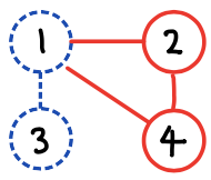
The data is generated from a time-varying vector autoregressive (tvVAR) model (see Section 2 for details), where components and are the sources of nonstationarity, i.e. they are affected by their own past through a (smoothly) time-varying parameter. In addition, component affects component . Component and affect each other in a time-invariant way. Component is also affected by and component and are affected through . As a result, components and inherit the nonstationarity from the sources and . As far as we are aware, there currently does not exist tools that adequately describe the nuanced differences in their dependencies and nonstationarity. Our aim in this paper is to capture these relationships in the form of the schematic diagram in Figure 1(b). We note that the tvVAR model is a special case of our general framework, which does not make any explicit assumptions on the data generating process.
It is interesting to contrast the networks constructed using the “dynamically changing” approach developed in Wang et al. (2019) and Safikhani and Shojaie (2020) for change point VAR models with our approach. Both networks convey different information about the nonstationary time series. The “dynamically changing” network can be considered as local in the sense that it identifies regions of stationarity and constructs a directed graph over each of the stationary periods. While the graph in our approach is undirected and yields global information about relationships between the nodes.
In order to connect the proposed framework to the current literature, we conclude this section by briefly reviewing the existing graphical modeling frameworks for Gaussian random vectors (GGM) and multivariate stationary time series (StGM). In Section 2 we lay the foundations for our nonstationary graphical models (NonStGM) approach. In particular, we formally define the notions of conditional noncorrelation and stationarity of nodes, edges, and subgraphs in terms of zero and Toeplitz embeddings of an infinite dimensional inverse covariance operator. We show that this framework offers a natural generalizations to existing notions of conditional noncorrelation in GGM and StGM. It should be emphasized that we do not assume that the underlying time series is Gaussian. All the relationships that we describe are in terms of the partial covariance and therefore apply to any multivariate time series whose covariance exists. In Section 3, we switch to Fourier domain and show that the conditional noncorrelation and nonstationarity relationships are explicitly encoded in the sparsity pattern of the integral kernel of the inverse covariance operator. This connection opens the door to learning the graph structure from finite length time series data with the discrete Fourier transforms (DFT). In Section 4 we focus on locally stationary time series. We show that by conducting nodewise regression of discrete Fourier transforms (DFT) of the multivariate time series across different Fourier frequencies it is possible to learn the network. Section 5 describes how the proposed general framework looks in the special case of tvVAR models, where the notions of conditional noncorrelation and nonstationarity are transparent in the transition matrix. Some numerical results are presented in Section 6 to illustrate the methodology. All the proofs for the results in this paper can be found in the Appendix.
Background. We outline some relevant works in graphical models and tests for stationarity that underpin the technical development of NonStGM.
Graphical Models. A graphical model describes the relationships among the components of a -dimensional system in the form of a graph with a set of vertices , and an edge set containing pairs of system components which exhibit strong association even after conditioning on the other components.
The focus of GGM is on the conditional independence relationships in a -dimensional (centered) Gaussian random vector . The non-zero partial correlations , defined as and also encoded in the sparsity structure of the precision matrix , are used to define the edge set . The task of graphical model selection, i.e. learning the edge set from finite sample, is accomplished by estimating with a penalized likelihood estimator as in graphical Lasso (Friedman et al. (2008)), or by nodewise regression (Meinshausen and Bühlmann (2006)) where each component of the random vector is regressed on the other components.
Switching to the time series setting, consider , a -dimensional time series with autocovariance function . Note that in future we usually use to denote the sequence . A direct adaptation of the GGM framework that estimates the contemporaneous precision matrix (see Zhang and Wu (2017); Qiu et al. (2016)) does not provide conditional relationships between the entire time series. Brillinger (1996) and Dahlhaus (2000b) laid the foundation of graphical models in stationary time series, where the conditional relationships between the entire time series and is captured. They show that the inverse of the multivariate spectral density function explicitly encodes the conditional uncorrelated relationships. To be precise, for all if and only if and are conditionally uncorrelated, given all the other time series. The graphical model selection problem reduces to finding all pairs where for some . For Gaussian time series the graph is a conditional independence graph while for non-Gaussian time series the graph encodes partial correlation information. For brevity, we refer to this approach as StGM (stationary time series graphical models). Estimation of is typically done using the Discrete Fourier transform of the time series (see Eichler (2008)). More recently, for relatively “large” , penalized methods such as GLASSO (Jung et al., 2015) and CLIME (Fiecas et al., 2019) have been used to estimate . This framework crucially relies on stationarity, in particular, the Toeplitz property of the autocovariance function , and is not immediately generalizable to the nonstationary case.
Testing for stationarity. There is a rich literature on testing for nonstationarity of a time series. Most methods are based on testing for invariance of the spectral density function or autocovariance function over time (see Priestley and Subba Rao (1969), Paparoditis (2009), Nason (2013) to name but a few). An alternative approach is based on the fact that the Discrete Fourier Transform at certain frequencies is close to uncorrelated for stationary time series. Epharty et al. (2001), Dwivedi and Subba Rao (2011), Jentsch and Subba Rao (2015), Aue and van Delft (2020) use this property to test for nonzero correlation between DFTs of different frequencies to detect for departures from stationarity. The above mentioned tests focus on the “marginal” notion of nonstationarity instead of the conditional notion defined in this paper. Tests for marginal nonstationarity are not equipped to delineate between direct and indirect nature of conditionally nonstationary relationships among the components of a multivariate time series. However, in this paper, we show that analogous to marginal tests, it is possible to utilize the Fourier domain to detect for different types of conditional (non)stationarity.
2 Graphical models and conditional stationarity
For a -dimensional nonstationary time series , all the pairwise covariance information are contained in the infinite set of autocovariance matrices , for . We aggregate this information into an operator , and show that its inverse operator captures meaningful conditional (partial) covariance relationships (Section 2.2). Leveraging this connection, we first define a graphical model, and conditional stationarity of its nodes, edges and subgraphs, in terms of the operator (Section 2.3). Then we show that these notions can be viewed as natural generalizations of the GGM and StGM frameworks (Sections 2.4 and 2.5). We start by introducing some notation that will be used to formally define these structures (this can be skipped on first reading). Let denote a -dimensional matrix, then we define , and .
2.1 Definitions and notation
We use and to denote the sequence space and the (column) sequence space respectively (vec denotes the vectorisation of a matrix). On the spaces and we define the two inner products (where denotes the complex conjugate), for and for , such that and are two Hilbert spaces. For let . For , we use to denote the entry in the matrix , which can be infinite dimensional and involve negative indices.
We consider the -dimensional real-valued time series , , where the univariate random variables , are defined on the probability space . We assume for all that this condition is not necessary in Sections 2 and 3, but it simplifies the exposition. Let denote all univariate random variables where , and for any we define the inner product . For every , we define the covariance and assume . Under this assumption, for all and . Let be the closure of the space spanned by . Since defines a Hilbert space, is also a Hilbert space. Therefore, by the projection theorem, for any closed subspace of , there is a unique projection of onto which minimises over all (see Theorem 2.3.1, Brockwell and Davis (2006)). We will use to denote this projection. In this paper, we will primarily use the following subspaces
where denotes the complement of .
Using the covariance we define the infinite dimensional matrix operator as where denotes an infinite dimensional submatrix with entries for all . For any , we define the (column) sequence where . For any we define the (column) sequence as
| (13) |
An infinite dimensional matrix operator, , is said to be zero, if all its entries are zero. An infinite dimensional matrix operator is said to be Toeplitz if its entries satisfy for all and for some sequence .
2.2 Covariance and inverse covariance operators
Within the nonstationary framework we require the following assumptions on to show that is a mapping from to (and later that is a mapping from to ). For stationary time series analogous assumptions are often made on the spectral density function (see Remark 2.1).
Assumption 2.1
Define , . Then
| (14) |
Assumption 2.1 implies that and also the coefficients of the inverse are square summable. It can be shown that if , then . This is analogous to a short memory condition for stationary time series. It is worth keeping in mind that cointegrated time series do not satisfy this condition. The theory developed in Sections 2 and 3 only require Assumption 2.1. However, to estimate the network stronger conditions on are required and these are stated in Section 4.
Under the above assumption , and since , , thus is a self-adjoint, bounded operator with , where denotes the operator norm: .
Remark 2.1
The core theme of GGM is to learn conditional (partial) covariances between two variables after conditioning on a set of other variables. These conditional relationships can be derived from the inverse covariance matrix. Now we will define a suitable inverse covariance operator and show how its entries capture the conditional relationships. We will define these conditional relations in terms of projections with respect to the -norm, this is equivalent to the least squares regression coefficients at the population level.
We consider the projection of onto , given by
| (15) |
with (note the coefficients are unique since is non-singular). Let , it can be shown that (see Appendix A.1). Analogous to finite dimensional covariance matrices, to obtain the entries of the inverse we use the coefficients of the projections of onto . For all , we define the -dimensional matrices as follows
| (18) |
Using we define the infinite dimensional matrix
| (19) |
Analogous to the definition of , we define .
Our next lemma shows that the operator is indeed the inverse of the covariance operator . We also state some upper bounds on its entries which will be useful in our technical analysis.
Lemma 2.1
PROOF In Appendix A.1.
2.3 Nonstationary graphical models (NonStGM)
The operators and provide us with the objects needed to formally define the edges in our network, and connect them to the notions of conditional uncorrelatedness and conditional stationarity.
At this point, we note an important distinction between edge construction in GGM and StGM, an issue that is crucial for generalizing graphical models to the nonstationarity case. In GGM, conditional uncorrelatedness between two random variables is defined after conditioning on all the other random variables in the system. On the other hand, in StGM, the conditional uncorrelatedness between two time series is defined after conditioning on all the other time series. This leads to two, potentially, different generalizations in the nonstationary setup. A direct generalization of the GGM framework would use the partial covariances , where . While a generalization of the StGM framework, would suggest using time series partial covariances , where .
To address this issue, we start by using the inverse covariance operator to define edges that encode conditional uncorrelatedness and (non)stationarity. We show that, as expected, these notions are a direct generalization of the GGM framework. Then we present a surprising result (Theorem 2.2), that the encoding of the partial covariances in terms of the operator remains unchanged even if we adopt the StGM notion of partial covariance, i.e. the conditionally uncorrelated and conditionally (non)stationary nodes, edges, subgraphs are preserved under the two frameworks.
We now define the network corresponding to the multivariate time series. Each edge in our network will have an indicator to denote conditional invariance and conditional time-varying, a new notion we now introduce. The edge set will contain all pairs where and are conditionally correlated. The edge set will also contain self-loops, that convey important information about the network. We start by formally defining the notions of conditional noncorrelation and (non)stationarity. This is stated in terms of the submatrices of .
Definition 2.1 (Nonstationary network)
Conditional covariance and (non)stationarity of the components of a -dimensional nonstationary time series are represented using a graph , where is the set of nodes, and is a set of undirected edges (), and includes self-loops of the form .
-
•
Conditional Noncorrelation The two time series and are conditionally uncorrelated if . As in GGM and StGM, this is represented by the absence of an edge between nodes and in the network, i.e. .
-
•
Conditionally Stationary Node The time series is conditionally stationary if is Toeplitz operator. We denote this using a solid self-loop around the node .
-
•
Conditionally Time-invariant Edge If and is a Toeplitz operator, then is a time invariant edge. We represent a conditionally time-invariant edge in our network with a solid edge.
-
•
Conditionally Stationary Subgraph A subnetwork of nodes is a called a conditionally stationary subgraph if for all , are Toeplitz operators i.e. is a block Toeplitz operator.
As a special case of the above, we call a conditionally stationary subgraph of order two (consisting of the nodes ) a conditionally stationary pair if and are Toeplitz.
-
•
Conditionally Nonstationary Node/Time-varying Edge: (i) If is not Toeplitz then is conditionally nonstationary. (ii) For , if is not Toeplitz then has a conditionally time-varying edge.
We represent conditional nonstationary nodes using a dashed self-loop and a conditionally time-varying edge with a dashed edge.
In Section 5 we show how the parameters of a general tvVAR model are related to the operator , and can be used to identify the network structure in NonStGM. As a concrete example, below we describe the network corresponding to the tvVAR considered in the introduction.
Example 2.1
Consider the following tvVAR(1) model for a -dimensional time series
where are independent random variables (i.i.d) with , and , are smoothly varying functions of . The four time series are marginally nonstationary, in the sense that for each , the time series is second order nonstationary.
The inverse operator and network corresponding to is given below and is deduced from the transition matrix (the explicit connection between and is given in Section 5). Note that red and blue denote Toeplitz and non-Toeplitz matrix operators respectively.
Connecting the transition matrix to the network The connections between the nodes is because node is connected to node (if for some ), node (if ) and node 2 (if ). By a similar argument, nodes and are connected (if or ).
The nonstationarity of the multivariate time series is due to the time-varying parameters and . Specifically, the parameter is the reason that node is nonstationary, and by a similar argument the time-varying parameter is the reason node is nonstationary. Since the coefficients on the second and fourth columns are not time-varying, nodes and have “inherited” their nonstationarity from nodes and . Thus nodes and are conditionally stationary whereas nodes and are conditionally stationary. The connections between nodes to and to are time-invariant because and are time-invariant respectively.
Remark 2.2 (Connection to GGM)
Let . It is clear that the density of the infinite dimensional vector is not well defined. However, we can informally view the joint density (at least in the Gaussian case) as “being proportional to”
This is analogous to the representation of multivariate Gaussian vector in terms of its inverse covariance. Using the above representation we conjecture that the above notions of conditional correlation/stationarity/nonstationarity can be generalized to time series which is not necessarily continuous valued, for example binary valued time series.
2.4 NonStGM as a generalization of GGM
We start by defining partial covariances in the spirit of the definition used in GGM but for infinite dimensional random variables. This is defined by removing two random variables from the spanning set of
| (22) |
Note that for the case and the above reduces to
| (23) |
In the discussion below we refer to the infinite dimensional conditional covariance matrices and . In GGM the partial covariances are encoded in the precision matrix. In a similar spirit, we show that is encoded in the inverse covariance operator .
Lemma 2.2
PROOF See Appendix A.2.
An immediate consequence of Lemma 2.2 is that the notions of conditional noncorrelation and conditional stationarity can be equivalently defined in terms of the properties of the partial covariances . In particular, conditional noncorrelation between the two series and translates to zero , while conditional stationarity of the pair translates to Toeplitz structures on , and . It is worth noting that the Toeplitz structure of (the partial covariance of ) captured in our framework is an important property, viz., the conditional (non)stationarity of a node. A similar role on the diagonal entries of the precision or spectral precision matrices ( or ) is absent in both the classical GGM and StGM frameworks.
Proposition 2.1 (NonStGM in terms of )
PROOF See Appendix A.2.
2.5 NonStGM as a generalization of StGM
Now we define the time series partial covariance analogous to that used in StGM. We recall that the classical time series definition of partial covariance in a multivariate time series evaluates the covariance between two random variables and , after conditioning on all random variables in the component series . In other words, we exclude the entire time series and from the conditioning set.
Formally, for any , we define the residual of after projecting on as
In the definitions below we focus on the two sets and . We mention that the set is not considered in StGMM but plays an important role in NonStGM. Using the above, we define the edge partial covariance
| (37) |
and node partial covariance
| (38) |
We will show that the partial covariance in (37) and (38) are closely related to the partial covariance in (22). In Lemma 2.2 we have shown that the partial correlations define the entries of the operator . We now connect the time series definition of a partial covariance to the operator . Before we present the equivalent definitions of our nonstationary networks in terms of the time series partial covariances , we show that can be expressed in terms of the inverse covariance operator .
Theorem 2.1
PROOF See Appendix A.3.
A careful examination of the expressions for the GGM covariance given in Lemma 2.2 with the StGM covariance given in shows they are very different quantities. Therefore, it is suprising that despite these stark differences they preserve the same structures. More precisely, in Proposition 2.1 we showed that Definition 2.1 had a clear interpretation in terms of . We show below that the network definition given in Definition 2.1 can be interpreted in terms of the conditional dependence (or residuals) of the time series. The fact that two very different conditional covariance definitions lead to the same conditional graph is due to the property that infinite dimensional Toeplitz operators remain Toeplitz even after inversion and multiplication with other Toeplitz operators.
Theorem 2.2
[NonStGM in terms of ] Suppose Assumption 2.1 holds. Let , and be defined as in (37) and (38) respectively. Then
-
(i)
Conditional noncorrelation iff for all and .
-
(ii)
Conditionally stationary node is a Toeplitz operator iff for all and , .
-
(iii)
Conditionally stationary pair , and are Toeplitz iff for all and , , and .
PROOF See Appendix A.3.
We show in the following result that the time series partial covariances can be used to define conditional stationarity of a subgraph containing three or more nodes.
Corollary 2.1 (Conditionally stationary subgraph)
Let be a subset of and denote the complement of . Suppose for all , are Toeplitz (including the case ). Then is a conditionally stationary subgraph where
with
PROOF See Appendix A.3.
3 Sparse characterisations within the Fourier domain
For general nonstationary processes it is infeasible to estimate the operator and learn its network within the time domain. The problem is akin to StGM, where it is difficult to learn the graph structure in the time domain by studying all the autocovariance matrices. Estimation is typically carried out in the Fourier domain by detecting conditional independence from the zeros of . Following the same route, we will switch to the Fourier domain and construct a quantity that can be used to “detect zeros and non-zeros”. In addition, within the Fourier domain we will define meaningful notions of weights/strengths of conditionally stationary nodes and pairs that are analogous to well-known partial spectral coherence measures used in StGM.
Notation We first summarize some of the notation we will use in this section. We define the function space of square integrable functions as all complex functions where if . We define the function space of all square summable vector complex functions , where if for all . For all we define the inner-product , where . Note that is a Hilbert space. We use to denote the Dirac delta function and set .
3.1 Transformation to the Fourier domain
In this section we summarize results which are pivotal to the development in the subsequent sections. This section can be skipped on first reading.
To connect the time and Fourier domain we define a transformation between the sequence and function space. We define the functions and
| (43) |
It is well known that and are isomorphisms between and (see, for example, Brockwell and Davis (2006), Section 2.9). For the transformations and where are isomorphisms between and . Often we use that . These two isomorphims will provide a link between the infinite dimensional matrix operators defined in the time domain to an equivalent operator in the Fourier domain.
Let , if is a bounded operator, then standard results show that is a bounded operator (see Conway (1990), Chapter II). is an integral operator, such that for all
| (44) |
and is the -dimensional matrix integral kernel where
To understand how and are related we focus on the case and note that the entry of the infinite dimensional matrix is
Remark 3.1 (Connection with covariances and stationary time series)
We note if were a covariance operator of a univariate time series with integral kernel then
| (45) |
where is the Loève dual frequency spectrum. The Loève dual frequency spectrum is used to describe nonstationary features in a time series and has been extensively studied in Gladyšev (1963), Lund et al. (1995), Lii and Rosenblatt (2002), Jensen and Colgin (2007), Hindberg and Olhede (2010), Olhede (2011), Olhede and Ombao (2013), Gorrostieta et al. (2019), Aston et al. (2019).
is a formal representation and typically it will not be a well defined function over , as it is likely to have singularities. Despite this, it has a very specific sparsity structure when the operator is Toeplitz. For the identification of nodes and edges in the nonstationary networks it is the location of zeros in that we will exploit. This will become apparent in the following lemma due to Toeplitz (1911) (we state the result for the case ).
Lemma 3.1
Suppose is an infinite dimensional bounded matrix operator . The matrix operator is Toeplitz iff the integral kernel associated with has the form
where and is the Dirac delta function.
PROOF See Appendix B.1 for details.
The crucial observation in the above lemma is that for iff is a Toeplitz matrix. Below we generalize the above to the case that (and its inverse) is a block Toeplitz matrix operator.
Lemma 3.2
Suppose that is an infinite dimensional, symmetric, block matrix operator where with and is Toeplitz. Then the integral kernel associated with is where is a matrix with entries . Further the integral kernel associated with is .
PROOF In Appendix B.1.
From now on we say that the kernel is diagonal if it can be represented as .
We use the operators and to recast the covariance and inverse covariance operators of a multivariate time series within the Fourier domain. We recall that is the covariance operator of the time series and by using (44) is an integral operator with matrix kernel where .
In the case that is second order stationary, then where is the spectral density matrix of . However, if is second order nonstationary, then by Lemma 3.1 at least one of the kernels will be non-diagonal. The dichotomy that the mass of lies on the diagonal if and only if the underlying process is multivariate second order stationary is used in (Epharty et al., 2001; Dwivedi and Subba Rao, 2011; Jentsch and Subba Rao, 2015) to test for second order stationarity.
3.2 The nonstationary inverse covariance in the Fourier domain
The covariance operator and corresponding integral kernel does not distinguish between direct and indirect nonstationary relationships. We have shown in Section 2 that conditional relationships are encoded in the inverse covariance . Therefore in this section we study the properties of the integral kernel corresponding to . Under Assumption 2.1, is a bounded operator, thus is a bounded operator defined by the matrix kernel where
| (46) |
and
| (47) |
Note that under Assumption 2.1 , this implies for all that the sequence , thus . As far as we are aware, neither nor haven been studied previously. But can be viewed as the inverse covariance version of the time-varying spectrum that is commonly used to analyze nonstationary covariances (see Priestley (1965), Martin and Flandrin (1985), Dahlhaus (1997), Birr et al. (2018)). We observe that is Toeplitz if and only if does not depend on .
In the following theorem we show that defines a very clear sparsity pattern depending on the conditional properties of . This will allow us to discriminate between different types of edges in a network. In particular, zero matrices map to zero kernels and Toeplitz matrices map to diagonal kernels.
Theorem 3.1
Suppose Assumption 2.1 holds. Then
-
(i)
Conditionally noncorrelated are conditionally noncorrelated iff
for all . -
(ii)
Conditionally stationary node is conditionally stationary iff the integral kernel is diagonal.
-
(iii)
Conditionally time-invariant edge The edge is conditionally time-invariant iff the integral kernel is diagonal.
PROOF In Appendix B.2.
These equivalences show that conditional noncorrelatedness and stationarity relationships in the graphical model, as defined by the operator, are encoded in the object . This provides the foundation for an alternate route to learning the graph structure in the frequency domain.
Example 3.1
We return to tvAR model described in Example 2.1. In Figure 2 we give a schematic illustration of the matrix in the frequency domain

3.3 Partial spectrum for conditionally stationary time series
So far we have considered the construction of an undirected, unweighted network which encodes the conditional uncorrelation and nonstationarity properties of time series components. In practice, we would be interested in assigning weights to network edges that represent the strength or magnitude of these conditional relationships. This will also be useful for learning the graph structure from finite samples. In GGM, partial correlation values are used to define edge weights, In StGM the partial spectral coherence (the frequency domain analogue of partial correlation) is used to define suitable edge weights.
We now define the notion of partial spectral coherence for conditionally stationary time series. We start by interpreting and , defined in (47), in the case that the node or edge is conditionally stationary. In the following proposition we relate these quantities to the partial covariance . Analogous to the definition of we define the partial correlation
| (48) |
Using the above we obtain an expression for and in the case that an edge or a node is conditionally stationary.
Theorem 3.2
PROOF In Appendix B.2.
For StGM, the partial spectral coherence is typically defined in terms of the Fourier transform of the partial time series covariances (see Priestley (1981), Section 9.3, and Dahlhaus (2000b)). We now show that an analogous result holds in the case of conditional stationarity.
Theorem 3.3
Suppose Assumption 2.1 holds.
-
(i)
If the node is conditionally stationary, then
-
(ii)
If is a conditionally stationary pair, then
PROOF In Appendix B.2.
The above allows us to define the notion of spectral partial coherence in the case that underlying time series is nonstationary. We recall that the spectral partial coherence between and for stationary time series is the standardized spectral conditional covariance (see Dahlhaus (2000b)). Analogously, by using Theorem 3.3(ii) the spectral partial coherence between the conditionally stationary pair is
| (50) |
In Appendix F we show how this expression is related to the spectral partial coherence for stationary time series.
3.4 Connection to node-wise regression
In Lemma 2.1 we connected the coefficients of to the coefficients in a linear regression. The regressors are in the spanning set of . In contrast, in node-wise regression each node is regressed on all of the other nodes (the coefficients in this regression can also be connected to the precision matrix). We now derive an analogous result for multivariate time series. In particular, we regress the time series at node () onto all the other time series (excluding node i.e. the spanning set of ) and connect these to the matrix . These results can be used to encode conditions for a conditionally stationary edge in terms of the regression coefficients. Furthermore, they allow us to deduce the time series at node conditioned on all the other nodes (if the time series is Gaussian).
The best linear predictor of given the “other” time series is
| (51) |
We group the coefficients according to time series and define the infinite dimensional matrix with entries
| (52) |
In the lemma below we connect the coefficients in the infinite dimensional matrix to
PROOF See Appendix B.3.
In the following theorem we rewrite the conditions for conditional noncorrelation and conditional time-invariant edge in terms of node-regression coefficients.
Theorem 3.4
PROOF See Appendix B.3.
Below we show that the integral kernel associated with has a clear sparsity structure.
Corollary 3.1
Suppose Assumption 2.1 holds. Let be defined as in (53). Let denote the integral kernel associated with . Then
-
(i)
is a bounded operator.
-
(ii)
Conditionally noncorrelated are conditionally noncorrelated iff
. -
(iii)
Conditionally stationary pair are conditionally jointly stationary iff the kernels , and are diagonal.
PROOF In Appendix B.3.
We use the results above to deduce the conditional distribution of under the assumption that the time series is jointly Gaussian. The conditional distribution of given is Gaussian where
with and . Some interesting simplications can be made if the nodes and corresponding edges are conditionally stationary and time-invariant. If has a conditionally stationary node, then by Theorem 2.2(ii) the conditional variance will be stationary (Toeplitz). If, in addition, the conditionally stationary node is connected to the set of nodes and all the edge connections are conditionally time-invariant then by Theorem 3.4 the coefficients in the conditional expectation are shift invariant where
Therefore, if the node is conditionally stationary and all its connecting edges are conditionally time-invariant then the conditional distribution is stationary.
4 Learning the network from finite length time series
The network structure of is succinctly described in terms of . However, for the purpose of estimation, there are three problems. The first is that is a singular kernel making direct estimation impossible. The second is that for conditional nonstationary time series the structure of is not well defined. Finally, in practice we only observe a finite length sample . Thus our object of interest changes from to its finite dimensional counterpart (which we define below). For the purpose of network identification, we show that the finite dimensional version of inherits the sparse properties of . Moreover, in a useful twist, whereas is a singular kernel its finite dimensional counterpart is a well defined matrix, making estimation possible.
4.1 Finite dimensional approximation
To obtain the finite dimensional version of , we recall that the Discrete Fourier transform (DFT) can be viewed as the analogous version of the Fourier operator (defined in (43)) in finite dimensions. Let denote the -dimension DFT transformation matrix. It comprises of identical -dimension DFT matrices, which we denote as . Define the concatenated -dimension vector , where for . Then is a -dimension vector where with
| (54) |
Let , then . Our focus will be on the -dimensional inverse matrix
where and the above follows from the identity . Let where denotes the -dimensional sub-matrix of and denotes the th entry in the submatrix matrix . For future reference we define the -dimensional matrix . We show below that can be viewed as the finite dimensional version of .
The covariance matrix is a submatrix of the infinite dimensional . Unfortunately its inverse is not a submatrix of . As our aim is to show that the properties of the inverse covariance map to those in finite dimensions we will show that under suitable conditions can be approximated by a finite dimensional submatrix of . To do this we represent as submatrices each of dimension
| (55) |
Analogously, we define submatrices of each of dimension
| (56) |
where . Below we show that under suitable conditions, can be approximated well by . This result requires the following conditions on the rate of decay of the inverse covariances which is stronger than the conditions in Assumption 2.1.
Assumption 4.1
The inverse covariance defined in (18)
satisfy the condition
(for some
).
The conditions in Assumption 4.1 are analogous to those used in the analysis of stationary time series, where certain conditions on the rate of decay of the autocovariances coefficients are often used. Krampe and Subba Rao (2022) obtain an equivalence between the rate of decay on and . In particular, Krampe and Subba Rao (2022) Theorem 2.1, show that under Assumption 2.1 and if for some and all we have that (where denotes the spectral norm), then . Thus Assumption 4.1 holds.
In the lemma below we obtain a bound between the rows of and .
Theorem 4.1
PROOF See Appendix C.1.
The theorem above shows that the further lies from the two end boundaries of the sequence the better the approximation between and . For example when (recall that is fixed) . Using Theorem 4.1 we replace with to obtain the following approximation.
Proposition 4.1
PROOF See Appendix C.1.
4.2 Locally stationary time series
We showed in Proposition 4.1 that in the case the node or edge is conditional stationary or conditionally time-variant has a well defined structure; the diagonal dominates the off-diagonal terms (which are of order ). However, in the case of conditional nonstationary node/time-varying edge the precise structure of is not apparent, this makes detection of conditional nonstationarity difficult. In this section we impose some structure on the form of the nonstationarity. We will work under the canopy of local stationarity. It formalizes the notion that the “nonstationarity” in a time series evolves “slowly” through time. It is arguably one of the most popular methods for describing nonstationary behaviour and describes a wide class of nonstationarity; various applications are discussed in Priestley (1965), Dahlhaus and Giraitis (1998), Zhou and Wu (2009), Cardinali and Nason (2010), Kley et al. (2019), Dahlhaus et al. (2019), Sundararajan and Pourahmadi (2018), Ding and Zhou (2020), Ombao and Pinto (2021), to name but a few. We show below that for locally stationary time series has a distinct structure that can be detected.
The locally stationary process were formally proposed in Dahlhaus (1997). In the locally stationary framework the asymptotics hinge on the rescaling device , which is linked to the sample size. It measures how close the nonstationary time series is to an auxillary (latent) process which for a fixed is stationary over . More precisely, a time series is said to be locally stationary if there exists a stationary time series where
| (61) |
Thus for every , can be closely approximated by an auxillary variable (where ); see (Dahlhaus and Subba Rao, 2006; Subba Rao, 2006; Dahlhaus, 2012; Dahlhaus et al., 2019). However, as the difference between and grows, the similarity between and the auxillary stationary process decreases. This asymptotic device allows one to obtain well defined limits for nonstationary time series which otherwise would not be possible within classical real time asymptotics. Though the formulation in (61) is a useful start for analysing nonstationary time series, analogous to Dahlhaus and Polonik (2006), we require additional local stationarity conditions on the moment structure. Dahlhaus (2000a) and Dahlhaus and Polonik (2006) state the conditions in terms of bounds between and . Below we state similar conditions in terms of the inverse covariances and its stationary approximation counterpart.
Assumption 4.2
There exists a sequence such that and matrix function where
| (62) |
Further, the matrix function is such that (i)
,
(ii) , (iii) for
all and (iv)
.
Standard within the locally stationary paradigm should be indexed by (but to simplify notation we have dropped the ).
Theorem 3.3 in Krampe and Subba Rao (2022) shows that Assumption 4.2 is fulfilled by a large class of locally stationary time series under certain smoothness conditions on their covariance.
The above assumptions require that the entry wise derivative of matrix functions exists. This technical condition can be relaxed to include matrix functions of bounded variation (which would allow for change point models as a special case) similar to Dahlhaus and Polonik (2006).
The above assumptions allow for two important types of behaviour (i) conditionally stationary nodes and time-invariant edges where and (ii) conditional nonstationarity where the partial covariance between and (for fixed lag ) evolves “nearly” smoothly over .
4.3 Properties of under local stationarity
Typically, the second order analysis of locally stationary time series is conducted through its time varying spectral density matrix. This is the spectral density matrix corresponding to the locally stationary approximation , which we denote as . The time-varying spectral density matrix corresponding to is . In contrast, in this section our focus will be on the inverse , where by Lemma 3.2, is the Fourier transform of over the lags i.e.
| (63) |
We note that . We use Assumption 4.2 to relate to (defined in (47)). In particular, is an approximation of and
| (64) |
Thus the time-varying spectral precision matrix corresponding to is .
Our aim is to relate to . First we notice that is “local” in the sense that it is a time local approximation to the precision spectral density at time point . On the other hand, is “global” in the sense that it is based on the entire observed time series. However, we show below that is connected to , as it measures how evolves over time. These insights allow us to deduce the network structure from .
In the following lemma we show that the entries of the matrix can be approximated by the Fourier coefficients of , where
| (65) |
The Fourier coefficients fully determine the function . In particular (i) if all the Fourier coefficients are zero then (ii) if all the Fourier coefficients are zero except , then does not depend on . Using this, it is clear the coefficients hold information on the network. We summarize these properties in the following proposition.
Proposition 4.2
Suppose Assumptions 2.1, 4.1 and 4.2 hold. Let be defined as in (65). Then
-
(i)
and is a (asymptotically) conditionally noncorrelated edge iff for all and .
-
(ii)
is a (asymptotically) conditionally stationary node iff for all and .
-
(iii)
The edge is conditionally time-invariant iff asymptotically for all and .
PROOF in Appendix C.2.
Note that the above result is asymptotic in rescaled time (). We make this precise in the following proposition where we show that closely approximates the Fourier coefficients .
Proposition 4.3
Suppose Assumptions 2.1, 4.1 and 4.2 hold. Let be defined as in (65). Then
| (66) |
Further,
| (70) |
where the bound is uniform over all (and is in rescaled time).
Since , then (70) can be replaced with , and respectively.
PROOF in Appendix C.2.
Note we split into three separate cases due to the circular wrapping of the DFT, which is most pronounced when lies at the boundaries of the interval .
In Dwivedi and Subba Rao (2011) and Jentsch and Subba Rao (2015) we showed that the Fourier transform of the time-varying spectral density matrix decayed to zero as and was smooth over . In the following lemma we show that a similar result holds for the Fourier transform of the inverse spectral density matrix.
Proposition 4.4 (Properties of )
Suppose Assumption 4.2 holds. Then for all we have
| (71) |
and . Furthermore, for all and
| (74) |
where is a finite constant that does not depend on or .
PROOF in Appendix C.2.
The above results describe two important features in :
-
1.
For a given subdiagonal , changes smoothly along the subdiagonal, where denotes the th subdiagonal (). Analogous to locally smoothing the periodogram, to estimate the entries of from the DFTs we use the smoothness property and frequencies in a local neighbourhood to obtain multiple “near replicates”.
-
2.
For a given row , is large when is close to zero and decays the further it is from zero.
These observations motivate the regression method that we describe below for learning the nonstationary network structure.
4.4 Node-wise regression of the DFTs
In this section, we propose a method for estimating the entries of . The problem of learning the network structure from finite sample time series is akin to the graphical model selection problem in GGM, addressed by Dempster (1972) for the low-dimensional and Meinshausen and Bühlmann (2006) for the high-dimensional setting. In particular, the neighborhood selection approach of Meinshausen and Bühlmann (2006) regresses one component of a multivariate random vector on the other components with Lasso (Tibshirani, 1996), and uses non-zero regression coefficients to select its neighborhood, i.e. the nodes which are conditionally noncorrelated with the given component.
Assuming the multivariate time series is locally stationary and satisfies Assumption 4.2, we show that the nonstationary network learning problem can be formulated in terms of a regression of DFTs at a specific Fourier frequency on neighboring DFTs. Let denote the DFT of the time series at Fourier frequency , as defined in (54). We denote the -dimensional vector of DFTs at by , and use to denote the -dimensional vector consisting of all the coordinates of except .
We define the space (note that the coefficients in this space can be complex). Then
| (75) |
where we set . Let
| (76) |
The above allows us to rewrite the entries of in terms of regression coefficients. In particular,
| (79) |
Comparing the above with Proposition 4.3 for we have
where
| (83) |
Thus by using Proposition 4.4 we have
| (84) |
where is a finite constant. The benefit of these results is in the estimation of the coefficients . We recall (75) can be expressed as
where the above is due to the periodic nature of , which allows us to extend the definition to frequencies outside . By using the near Lipschitz condition in (84) if and are “close” then the coefficients of the projections and will be similar. This observation will allow us to estimate using the DFTs whose frequencies all lie in the -neighbourhood of (analogous to smoothing the periodogram of stationary time series). We note that with these quasi replicates the estimation would involve (where ) response variables and regressors. Even with the aid of sparse estimation methods this is a large number of regressors. However, Proposition 4.4 allows us to reduce the number of regressors in the regression. Since we can truncate the projection to a small number () of regressors about to obtain the approximation
Thus smoothness together with near sparsity of the coefficients make estimation of the entries in the high-dimensional precision matrix feasible.
For a given choice of and , and every value of , we define the -dimensional complex response vector , and the dimensional complex design matrix
Then the estimator
of is obtained by solving the complex lasso optimization problem
where , the sum of moduli of all the (complex) coordinates, and is a (real positive) tuning parameter controlling the degree of regularization. It is well-known (Maleki et al., 2013) that the above optimization problem can be equivalently expressed as a group lasso optimization over real variables, and can be solved using existing software. We use this property to compute the estimators in our numerical experiments.
From Proposition 4.2 we observe that the problem of graphical model selection reduces to learning the locations of large entries of for different Fourier frequencies . Furthermore, from equation (79) and (83) it is possible to learn the sparsity structure of from the regression coefficients (up to order ). In particular, there is an edge , i.e. the components and are conditionally correlated, if is non-zero for some (within the locally stationary framework). Similarly, an edge between and is conditionally time-varying if is non-zero for some . In the above we have ignored the terms.
In view of these connections, we define two quantities involving the estimated regression coefficients whose sparsity patterns encode information on the graph structure. In particular, we aggregate the estimated regression coefficients across different Fourier frequencies into two weight matrices
| (86) | |||||
| (87) |
for graphical model selection in NonStGM. Two components and are deemed conditionally noncorrelated if both the and the off-diagonal elements of are small. In contrast, a node is deemed conditionally stationary if the element of is small. Similarly, an edge between and is deemed conditionally time-invariant if both the and the elements of is small. Note that our node-wise regression approach does not ensure that the estimated weight matrices are symmetric. However, following (Meinshausen and Bühlmann, 2006), one can formulate suitable “and” (or “or”) rule to construct an undirected graph, where an edge is present if the and entries are both large (or at least one of them is large).
5 Time-varying Vector Autoregressive Models
In this section we link the structure of the coefficients of the time-varying Vector Autoregressive (tvVAR) process with the notion of conditional noncorrelation and conditional stationarity. This gives a rigourous understanding of certain features in a tvVAR model.
The time-varying VAR (tvVAR) model is often used to model nonstationarity (see Subba Rao (1970), Dahlhaus (2000a), Dahlhaus and Polonik (2006), Zhang and Wu (2021), Safikhani and Shojaie (2020)). A time series is said to have a time-varying VAR representation if it can be expressed as
| (88) |
where are i.i.d random vectors with and . For simplicity, we have centered the time series as the focus is on the second order structure of the time series. We assume that (88) has a well defined time-varying moving average representation as its solution (we show below that this allows the inverse covariance to be expressed in terms of ). We show below that the inverse covariance matrix operator corresponding to (88) has a simple form that can easily be deduced from the VAR parameters.
5.1 The tvVAR model and the nonstationary network
In this section we obtain an expression for in terms of the tvVAR parameters.
Let and denote the corresponding covariance operator as defined in (13). Let denote the Cholesky decomposition of such that (where denotes the transpose of ). To obtain we use the Gram-Schmidt orthogonalisation. We define the following matrices;
Using we define the infinite dimensional, block, lower triangular matrix where the th block of is defined as for all . Define , then is defined as
By definition of (88) it can be seen that are uncorrelated random vectors with . From this, it is clear that is the inverse of a rearranged version of . We use this to deduce the inverse . We define as
| (90) |
The inverse of is , where is defined by substituting (90) into (19).
We now focus on the case and derive conditions for conditional noncorrelation and stationarity. In this case, the suboperators have the entries
| (93) |
where denotes the column of the matrix and the standard dot product on . Using the above expression for , the parameters of the tvVAR model can be connected to conditional noncorrelation and conditional stationarity:
-
(i)
Conditional noncorrelation If for all the non-zero entries in the columns and do not coincide, then and are conditionally noncorrelated.
-
(ii)
Conditionally stationary node If for all , the columns do not depend on then the node is conditionally stationary and the submatrix simplifies to
-
(iii)
Conditionally time-invariant edge If for all and the dot products do not depend on and and does not depend on then is Toeplitz where
for all .
There can arise situations where some and depend on , but the corresponding node or edge is conditionally stationary or time-invariant. This happens when there is a cancellation in the entries of . However, these cases are quite exceptional.
In Appendix D we state conditions on the tvVAR process such that Assumptions 2.1, 4.1 and 4.2 are satisfied.
Remark 5.1 (The time-varying AR approximation of locally stationary time series)
In Krampe and Subba Rao (2022), Theorem 3.3 it is shown that if a multivariate nonstationary time series satisfies certain second order locally stationary conditions, then the time series has a tvAR representation with nearly smooth VAR parameters i.e.
where is a lower triangular matrix, and are Lipschitz continuous and are uncorrelated random variables with . Using and it would be possible to determine the approximate network of a nonstationary time series based on the conditions (i,ii,iii) stated above.
6 Numerical Experiments
We demonstrate the applicability of node-wise regression in selecting NonStGM on two systems of multivariate time series, a small () dimensional tvVAR(1) process described in Example 2.1, and a large () dimensional tvVAR(1) process.
6.1 Small System

We simulate the dimensional tvVAR(1) system described in Example 2.1, where all the time-invariant parameters set to and with observations. The two time-varying parameters and change from to as varies from to according to the function . Using the results from Section 5.1, nodes are conditionally nonstationay and the edge is conditionally time-varying. On the other hand, the nodes are conditionally stationary and the edge , and (1,4) are conditionally time-invariant. As Figure 1(a) shows, these nuanced relationships are not prominent from the four time series trajectories.
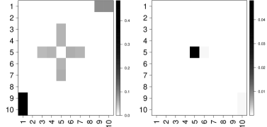
We perform node-wise regression of DFTs with and . The tuning parameters in the individual group lasso regressions were selected using cross-validation. The estimated regression coefficients were used to construct the weight matrices and . The heat maps of these weight matrices, aggregated over replicates, are displayed in Figure 3.
The true graph structure (left) has two conditionally nonstationary nodes , and two stationary nodes . A heat map of (middle) clearly shows the edges , and capturing conditional noncorrelation in the true graph structure. The heat map of (right) shows the conditionally nonstationary nodes and on the diagonal. The conditionally time-varying edge is also clearly visible on this heat map.
6.2 Large System
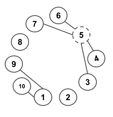
We now consider a larger system of . The data generating process is tvVAR(1) . Here . Non-zero time-invariant entries of the transition matrix are constant functions as follows: for all , . The only time-varying entry is , where decays exponentially from to as varies from to according to the function . As we can see from the structure of (and the true graph structure in the left panel of Figure 4), this network has two connected components and two isolated nodes ( and ). These two nodes are independent of the other nodes, and are treated as the “control”. The component consisting of is stationary (due to time invariant AR parameters). On the other hand, the component is nonstationary. However, the source of nonstationarity is node which permeates through to nodes and . Thus the four nodes and are conditionally stationary (due to time-invariant parameters).
We simulate observations from this system, and perform node-wise regression of DFTs with and . The tuning parameters in the individual group lasso regressions were selected using cross-validation. The estimated regression coefficients were used to construct the weight matrices and . The heat maps of these weight matrices, aggregated over replicates, are displayed in Figure 4.
We observe that the edges for both components and are visible in the heat map of (middle). As expected the isolated nodes do not show up. The heat map of (right) correctly identifies node as conditionally nonstationary.
Conclusion
We introduced a general graphical modeling framework for describing conditional relationships among the components of a multivariate nonstationary time series using an undirected network. In this network, absence of an edge corresponds to conditional noncorrelation relationships, as is common in GGM and StGM. An additional node or edge attribute (dashed or solid) further describes a newly introduced notion of conditional nonstationarity, which can be used to provide a parsimonious description of nonstationarity inherent in the overall system. We showed that this framework is a natural generalization of the existing GGM and StGM network. Under the locally stationary framework, we proposed methods to learn the nonstationary graph structure from finite-length time series in the Fourier domain. Numerical experiments on simulated data demonstrate the feasibility of our proposed method.
For stationary time series, there is well-established asymptotic theory for spectral density matrix estimators (see, e.g. (Woodroofe and Van Ness, 1967; Brillinger, 2001; Wu and Zaffaroni, 2018; Rosuel et al., 2021)). To estimate the inverse of moderate to high-dimensional spectral density matrices, penalized estimation methods for detecting non-zero off-diagonal entries (Fiecas et al., 2019) have shown promise. These methods are based on learning the conditional correlation structure of the DFTs at different nodes at the same frequency. Using the results in Section 4.4 we conjecture that the nonstationary network can be estimated by learning the non-zero coefficients of node-wise DFT regression across different frequencies. In future work, we hope to develop a complete statistical theory for graphical model estimation and inference.
Acknowledgements
SB and SSR acknowledge the partial support of the National Science Foundation (grants DMS-1812054 and DMS-1812128). In addition, SB acknowledges partial support from the National Institute of Health (grants R01GM135926 and R21NS120227). The authors thank Gregory Berkolaiko for several useful suggestions and Jonas Krampe for careful reading. The authors thank the Associate Editor and two anonymous referees for their thoughtful comments and suggestions which substantially improved the paper.
References
- Andersson et al. (2001) Steen A Andersson, David Madigan, and Michael D Perlman. Alternative markov properties for chain graphs. Scandinavian journal of statistics, 28(1):33–85, 2001.
- Aston et al. (2019) J. Aston, D. Dehay, J-M. Dudek, A. Freyermuth, D. Szucs, and L. Colling. (dual-frequency)-dependent dynamic functional connectivity analysis of vidual working memory capacity. Preprint: Hal-021335535, 2019.
- Aue and van Delft (2020) A. Aue and A. van Delft. Testing for stationarity of functional time series in the frequency domain. Ann. Statist., 48:2505–2547, 2020.
- Basu and Michailidis (2015) S. Basu and G. Michailidis. Regularized estimation in sparse high-dimensional time series models. Ann. Statist., 43(4):1535–1567, 2015.
- Berkolaiko and Kuchment (2020) G. Berkolaiko and P. Kuchment. Spectral shift via literal pertubation. arXiv preprint arXiv:2011.11142, 2020.
- Birr et al. (2018) S. Birr, H. Dette, M. Hallin, T. Kley, and S. Volgushev. On Wigner–Ville spectra and the uniqueness of time-varying copula-based spectral densities. J. Time Series Anal., 39:242–250, 2018.
- Böhm and von Sachs (2009) H. Böhm and R. von Sachs. Shrinkage estimation in the frequency domain of multivariate time series. J. Multivar. Anal., 100(5):913–935, 2009.
- Böttcher and Grudsky (2000) Albrecht Böttcher and Sergei M. Grudsky. Toeplitz matrices, asymptotic linear algebra, and functional analysis. Birkhäuser Verlag, Basel, 2000.
- Brillinger (1996) D. R. Brillinger. Remarks concerning graphical models for time series and point processes. R de Econometrica, 16:1–23, 1996.
- Brillinger (2001) David R. Brillinger. Time series: Data Analysis and theory, volume 36 of Classics Appl. Math. SIAM, Philadelphia, PA, 2001.
- Brockwell and Davis (2006) Peter J. Brockwell and Richard A. Davis. Time series: theory and methods. Springer Series in Statistics. Springer, New York, 2006. Reprint of the second (1991) edition.
- Cardinali and Nason (2010) A. Cardinali and G.P. Nason. Costationarity of locally stationary time series. J. Time Ser. Econom., 2(2):Art. 1, 33, 2010.
- Chau and von Sachs (2020) J. Chau and R. von Sachs. Intrinsic wavelet regression for surfaces of Hermitian positive definite matrices. J. Am. Stat. Assoc., 2020.
- Conway (1990) J. B. Conway. A course in functional analysis. Springer, New York, 1990.
- Dahlhaus (1997) R. Dahlhaus. Fitting time series models to nonstationary processes. Ann. Statist., 25(1):1–37, 1997.
- Dahlhaus (2000a) R. Dahlhaus. A likelihood approximation for locally stationary processes. Ann. Statist., 28(6):1762–1794, 2000a.
- Dahlhaus (2000b) R. Dahlhaus. Graphical interaction models for multivariate time series. Metrika, 51(2):157–172, 2000b.
- Dahlhaus (2012) R. Dahlhaus. Handbook of Statistics, volume 30, chapter Locally Stationary processes, pages 351–413. Elsevier, 2012.
- Dahlhaus and Eichler (2003a) R. Dahlhaus and M. Eichler. Causality and graphical models in time series analysis. In Highly structured stochastic systems, volume 27 of Oxford Statist. Sci. Ser., pages 115–144. 2003a.
- Dahlhaus and Giraitis (1998) R. Dahlhaus and L. Giraitis. On the optimal segment length for parameter estimates for locally stationary time series. J. Time Series Anal., 19:629–655, 1998.
- Dahlhaus and Polonik (2006) R. Dahlhaus and W. Polonik. Nonparametric quasi-maximum likelihood estimation for Gaussian locally stationary processes. Ann. Statist., 34(6):2790–2824, 2006.
- Dahlhaus and Subba Rao (2006) R. Dahlhaus and S. Subba Rao. Statistical inference of time varying ARCH processes. Ann. Statistics, 34:1074–1114, 2006.
- Dahlhaus et al. (1997) R. Dahlhaus, M. Eichler, and J. Sandühler. J. Neuroscience Methods, 77:93–107, 1997.
- Dahlhaus et al. (2019) R. Dahlhaus, S. Richter, and W. B. Wu. Towards a general theory for nonlinear locally stationary processes. Bernoulli, 25(2):1013–1044, 2019.
- Dahlhaus and Eichler (2003b) Rainer Dahlhaus and Michael Eichler. Causality and graphical models in time series analysis. Oxford Statistical Science Series, pages 115–137, 2003b.
- Davis et al. (2016) R.A. Davis, P. Zang, and T. Zheng. Sparse vector autoregressive modeling. J. of Computat. Graph. Statist., 25(4):1077–1096, 2016.
- Dempster (1972) A. P. Dempster. Covariance selection. Biometrics, pages 157–175, 1972.
- Diebold and Yılmaz (2014) F.X. Diebold and K. Yılmaz. On the network topology of variance decompositions: Measuring the connectedness of financial firms. J. Econometrics, 182(1):119–134, 2014.
- Ding and Zhou (2020) X. Ding and Z. Zhou. Estimation and inference for precision matrices of non-stationary time series. Ann. Statist., 48:2455–2477, 2020.
- Dwivedi and Subba Rao (2011) Y. Dwivedi and S. Subba Rao. A test for second order stationarity based on the Discrete Fourier Transform. J. Time Series Anal., 32:68–91, 2011.
- Eichler (2007) M. Eichler. Granger causality and path diagrams for multivariate time series. J. Econometrics, 137(2):334–353, 2007.
- Eichler (2008) M. Eichler. Testing nonparametric and semiparametric hypotheses in vector stationary processes. J. Multivariate Anal., 99:968–1009, 2008.
- Epharty et al. (2001) A. Epharty, J. Tabrikian, and H. Messer. Underwater source detection using a spatial stationary test. Journal of the Acoustical Society of America, 109:1053–1063, 2001.
- Fiecas et al. (2019) M. Fiecas, C. Leng, W. Liu, and Y Yu. Spectral analysis of high-dimensional time series. Electron. J. Stat., 13(2):4079–4101, 2019.
- Friedman et al. (2008) J. Friedman, T. Hastie, and R. Tibshirani. Sparse inverse covariance estimation with the graphical lasso. Biostatistics, 9(3):432–441, 2008.
- Gladyšev (1963) E. G. Gladyšev. Periodically and semi-periodically correlated random processes with continuous time. Teor. Verojatnost. i Primenen., 8:184–189, 1963.
- Gorrostieta et al. (2019) C. Gorrostieta, H. Ombao, and R. von Sachs. Time-dependent dual-frequency coherence in multivariate non-stationary time series. J. Time Series Anal., 40(1):3–22, 2019.
- Hindberg and Olhede (2010) H. Hindberg and S. C. Olhede. Estimation of ambiguity functions with limited spread. IEEE Transactions on Signal Processing, 58:2383–2388, 2010.
- Jensen and Colgin (2007) O. Jensen and L. Colgin. Cross-frequency coupling between neuronal oscillations. Trends in Cognitive Sciences, 11:267–269, 2007.
- Jentsch and Subba Rao (2015) C. Jentsch and S. Subba Rao. A test for second order stationarity of a multivariate time series. J. Econometrics, 185, 2015.
- Jung et al. (2015) A. Jung, G. Hannak, and N. Goertz. Graphical lasso based model selection for time series. IEEE Signal Processing Letters, 22(10):1781–1785, 2015.
- Kley et al. (2019) T. Kley, P. Preuss, and P. Fryzlewicz. Predictive, finite-sample model choice for time series under stationarity and nonstationarity. Electron. J. Stat., 13:3710–3774, 2019.
- Krampe and Subba Rao (2022) J. Krampe and S. Subba Rao. Inverse covariance operators of nonstationary multivariate time series. https://arxiv.org/abs/2202.00933, 2022.
- Künsch (1995) H.P. Künsch. A note on causal solutions for locally stationary AR-processes. Technical report, ETH, 1995.
- Lii and Rosenblatt (2002) K-S. Lii and M. Rosenblatt. Spectral analysis for harmonizable processes. Ann. Statist., 30(1):258–297, 2002.
- Lund et al. (1995) R. Lund, H. Hurd, P. Bloomfield, and R. Smith. Climatological time series with periodic correlation. Journal of Climate, 11:2787–2809, 1995.
- Lurie et al. (2020) D.J. Lurie, D. Kessler, D.S Bassett, R.F. Betzel, M. Breakspear, S. Kheilholz, A. Kucyi, R. Liégeois, M.A. Lindquist, and A. R. McIntosh. Questions and controversies in the study of time-varying functional connectivity in resting fmri. Network Neuroscience, 4(1):30–69, 2020.
- Maleki et al. (2013) A. Maleki, L. Anitori, Z. Yang, and R. G. Baraniuk. Asymptotic analysis of complex lasso via complex approximate message passing (camp). IEEE Trans. Inf. Theory, 59(7):4290–4308, 2013.
- Martin and Flandrin (1985) W. Martin and P. Flandrin. Wigner-Ville spectral analysis of nonstationary processes. IEEE Transactions on Acoustics, Speech, and Signal Processing, 33:1461–1470, 1985.
- Meinshausen and Bühlmann (2006) N. Meinshausen and P. Bühlmann. High-dimensional graphs and variable selection with the lasso. Ann. Statist., 34(3):1436–1462, 2006.
- Meyer et al. (2017) M. Meyer, C. Jentsch, and J.-P. Kreiss. Baxter’s inequality and sieve bootstrap for random fields. Bernoulli, 23(4B):2988–3020, 2017.
- Nason (2013) G.P. Nason. A test for second-order stationarity and approximate confidence intervals for localized autocovariances for locally stationary time series. J. Roy. Statist. Soc. (B), 75, 2013.
- Olhede (2011) S. C. Olhede. Ambiguity sparse processes. arXiv preprint arXiv:1103.3932v2.pdf, 2011.
- Olhede and Ombao (2013) S. C. Olhede and H. Ombao. Covariance of replicated modulated cyclical time series. IEEE Transactions on Signal Processing, 61:1944–1957, 2013.
- Ombao and Pinto (2021) H. Ombao and M. Pinto. Spectral dependence. https://arxiv.org/abs/2103.17240, 2021.
- Paparoditis (2009) E. Paparoditis. Testing temporal constancy of the spectral structure of a time series. Bernoulli, 15:1190–1221, 2009.
- Preti et al. (2017) M. G. Preti, T. AW Bolton, and D. Van De Ville. The dynamic functional connectome: State-of-the-art and perspectives. Neuroimage, 160:41–54, 2017.
- Priestley (1965) M. B. Priestley. Evolutionary spectra and non-stationary processes. J. Roy. Statist. Soc. (B), 27:204–37, 1965.
- Priestley (1981) M. B. Priestley. Spectral analysis and time series. Vol. 2. Academic Press, Inc. [Harcourt Brace Jovanovich, Publishers], London-New York, 1981. Multivariate series, prediction and control, Probability and Mathematical Statistics.
- Priestley and Subba Rao (1969) M. B. Priestley and T. Subba Rao. A test for non-stationarity of a time series. J. Roy. Statist. Soc. (B), 31:140–149, 1969.
- Qiu et al. (2016) H. Qiu, F. Han, H. Liu, and B. Caffo. Joint estimation of multiple graphical models from high dimensional time series. J. R. Statist. Soc. (B), 78(2):487, 2016.
- Rosuel et al. (2021) Alexis Rosuel, Philippe Loubaton, and Pascal Vallet. On the asymptotic distribution of the maximum sample spectral coherence of gaussian time series in the high dimensional regime. arXiv preprint arXiv:2107.02891, 2021.
- Safikhani and Shojaie (2020) A. Safikhani and A. Shojaie. Joint structural break detection and parameter estimation in high-dimensional non-stationary var models. J. Am. Stat. Assoc., (just-accepted):1–26, 2020.
- Subba Rao (2006) S. Subba Rao. On some nonstationary, nonlinear random processes and their stationary approximations. Adv. Appl. Probab., 38(4):1155–1172, 2006.
- Subba Rao (1970) T. Subba Rao. The fitting of non-stationary time-series models with time-dependent parameters. J. Roy. Statist. Soc. B, 32:312–22, 1970.
- Sun et al. (2018) Y. Sun, Y. Li, A. Kuceyeski, and S. Basu. Large spectral density matrix estimation by thresholding. arXiv preprint arXiv:1812.00532, 2018.
- Sundararajan and Pourahmadi (2018) R. R. Sundararajan and M. Pourahmadi. Stationary subspace analysis of nonstationary processes. J. Time Series Anal., pages 338–355, 2018.
- Tibshirani (1996) R. Tibshirani. Regression shrinkage and selection via the lasso. J. Roy. Statist. Soc. (B), 58(1):267–288, 1996.
- Toeplitz (1911) O. Toeplitz. Zur Theorie der quadratischen und bilinearen Formen von unendlichvielen Veränderlichen. Math. Ann., 70(3):351–376, 1911.
- Tretter (2008) Christiane Tretter. Spectral theory of block operator matrices and applications. Imperial College Press, 2008.
- Wang et al. (2019) D. Wang, Y. Yu, A. Rinaldo, and R. Willett. Localizing changes in high-dimensional vector autoregressive processes. arXiv preprint arXiv:1909.06359, 2019.
- Woodroofe and Van Ness (1967) Michael B Woodroofe and John W Van Ness. The maximum deviation of sample spectral densities. The Annals of Mathematical Statistics, pages 1558–1569, 1967.
- Wu and Zaffaroni (2018) Wei Biao Wu and Paolo Zaffaroni. Asymptotic theory for spectral density estimates of general multivariate time series. Econometric Theory, 34(1):1–22, 2018.
- Zhang and Wu (2017) D. Zhang and W. B. Wu. Gaussian approximation for high dimensional time series. Ann. Statist., 45:1895–1919, 2017.
- Zhang and Wu (2021) D. Zhang and W. B. Wu. Second-order asymptotics for high dimensional locally stationary processes. Ann. Statist., 49:233–254, 2021.
- Zhou and Wu (2009) Z. Zhou and W. B. Wu. Local linear quantile estimation for nonstationary time series. Ann. Statist., 37:2696–2729, 2009.
Appendix A Proofs for Section 2
A.1 Proofs of results in Section 2.2
We first show that . This ensures that and the operator is well defined (see (18)). We recall that
where . For all except let and let . For every define and . It is easily seen that
| (95) |
Since , by Assumption 2.1 we have
| (96) |
We use this result and the notation above to prove Lemma 2.1.
PROOF of Lemma 2.1 For we define the column vectors and . Using the notation introduced at the start of this section we have
Since minimises the mean squared error over all and , this gives rise to the normal equations
Comparing the above with , we observe that this proves and , thus . To prove that , we note that under Assumption 2.1, . Since is a self-adjoint operator, and .
To prove that we first focus on the case .
Since are submatrices on the diagonal of and , then it immediately follows that
. Therefore, since is self-adjoint (symmetric) we
have . By a similar argument .
To prove the result for we focus on the sub-matrix
Using the same argument to prove that it can be shown that . Thus for all we have . We use this bound below. We recall that an operator (matrix) is bounded if there exists a finite constant where for all we have , it follows that . Returning to , we will show that . For all we have
where . Thus , as required.
Finally, to prove that , we first prove that for every , we have . Define the sequence where we set and for and (zero sequence) for all . Then by definition of (which mainly consists of zeros except for one non-zero entry) we have
Thus for every we have . By the same argument for any and we have , this gives . This proves the claim.
Many of the results in this section use the block operator inversion identity (see Tretter (2008), page 35, and Berkolaiko and Kuchment (2020), Section 2.3)). For completeness we give the identity below. As we are working with covariance matrix operators we focus on symmetric/self-adjoint matrices. Suppose
and exists, then
| (103) |
where . We mention that is the Schur complement of of the matrix .
A.2 Proof of results in Section 2.4
There are different methods for proving the results in Section 2.4. One method is to use the properties of projections the other is to use decompositions of the infinite dimensional matrix . In this section we take the matrix decomposition route, as similar matrix decompositions form the core of the proofs in Section 2.5.
As the results in Section 2.4 concern the partial covariance between and given all the other random variables, we will consider a permuted version of and its inverse, where we bring the covariance structure of to the top left hand corner of the matrix. To avoid introducing new notation we label these permuted matrix operators as and . The variance of is
This embeds in the top left hand side of the operator , where
| (107) |
with ,
and
(we have
used the tilde notation in
to distinguish it from ). It is well
known that the Schur complement encodes the partial
covariance. Applying this to , the Schur
complement of in is
| (110) |
The above matrix (which we label as ) forms an important part of all the proofs in this section. As the entries in the variance matrix on the left hand side of (110) is quite long we replace it with some shorter notation for the conditional variances and covariances. Comparing (110) with (22) we observe that the off-diagonal is . However, the diagonal of has not been defined in Section 2.4. As this is the partial variance of after conditioning on everything but and we use the notation
| (111) |
To avoid confusion, we mention that this is different to the time series partial covariance defined in Section 2.5, where is the partial variance of after conditioning on all the other time series but time series and . Using the new notation we have
| (116) | |||||
Next we relate to the inverse . Using the block operator inversion (see (103)) we have
| (119) |
where is defined in (110). Comparing with the upper left block of , we connect the conditional variance of to the entries of . In particular
| (124) |
The identity (124) forms an important component in the proofs below.
Before we state the next lemma, we require the following notation for the partial correlation between and
| (125) |
Lemma A.1
PROOF. The proof of (126) is based on comparing and the ratio of the diagonal entries of the conditional variance in (124)
| (130) | |||||
| (133) |
We recall from (18) that
| (134) |
Furthermore, by comparing the entries in (130) we have
Thus evaluating ratio of the above gives
| (135) |
To prove (127) we decompose the projection of in terms of its projections onto the two space and . These two spaces are orthogonal and lead to a simple expression for the coefficient ;
| (136) | |||||
Using the orthogonality of the two projections we have
Replacing the covariance in with its correlation gives
| (137) |
This links the partial correlation to the projection coefficients. Finally, we substitute the identity (126) into (137) to give
This proves (127).
We use the above to prove Lemma 2.2.
PROOF of Lemma 2.2 By using (127) we connect to the precision matrix. Since
and by definition of in (19) we have
This proves (24). The proof of (29) immediately follows from (124).
PROOF of Proposition 2.1 The proof hinges on the identity in (124) for the separate cases and . For the case and using (124) it is clear that iff . Thus iff for all and , , this proves (i).
To prove (ii), we use (124) with and compare the entries of
| (140) | |||||
| (143) |
We first show that if is a symmetric, Toeplitz matrix, then is shift invariant (depends only on ). If is a symmetric, Toeplitz matrix, using that it is clear that does not depend on . We now study when . To show that only depends on we use that (due to being Toeplitz). Comparing the off-diagonal entries on the left and right hand side of (143) it follows that for all and .
Next we show the converse, that is if for all and ; then is a symmetric, Toeplitz matrix. First the diagonal, since it is clear that the diagonal does not depend on . Next we show that if for all and ; , then
-
(a)
only depends on .
-
(b)
The conditional variance only depends on . Note that this is not in the statement of the theorem, but is a useful by product of the proof.
Comparing the entries of the matrices in (143) we have
| (144) | |||||
| (145) | |||||
| (146) |
We first show that only depends on . To reduce notation, we set the entries on the diagonal of to and let . Substituting this into (145) gives
The above is quadratic equation in . Thus we can express in terms of and ;
Note that is part of the solution and not due to the positivity condition in (146). This proves that is a symmetric, Toeplitz matrix. This proves (a) and (ii) in the lemma. To prove (b), we use (144) and observe that the right hand side depends only on , thus proving that only depends on .
To prove (iii) we use (124) with . From (124) it immediately follows that if and are Toeplitz, then only depends on the lag .
Conversely, to prove that is Toeplitz given that for all and ; . , , we use the same strategy used to prove (ii). This yields the solution
which proves that is Toeplitz. Thus proving the result.
A.3 Proof of results in Section 2.5
To prove the results in Section 2.5 we follow a similar strategy to the proofs of Section 2.4, but permute the submatrices in rather than the individual entries in . The proofs in this section are less technical than those in Section 2.4.
Define the two non-intersecting sets and its complement where . We now obtain an expression for the covariance of after removing their linear dependence on . To do so, we define the submatrix where we note that
A block permuted version of with in the top left hand corner is
where , . By using standard results, the conditional variance of given is the Schur complement of of :
| (148) |
Using the above, entrywise for all and , we have
We now relate the conditional variance (defined in (148)) to the matrix . Using the block operator inversion identity in (103) we have
| (151) |
where is defined in (148).
To prove (i) we let . By using (148) we have
| (152) |
Thus entrywise by definition we have , this proves (i).
To prove (ii) we let . By using (148) and (103) we have
where the above follows from (103). Comparing entries in the above matrix gives
This proves (ii).
PROOF of Theorem 2.2 Before we prove the result, we note the following invariance properties of (infinite dimension) Toeplitz operators. If and are bounded Toeplitz operators then (a) is Toeplitz (b) if is Toeplitz and has a bounded inverse, then is Toeplitz; these results are a consequence of Toeplitz Theorem, Toeplitz (1911). It is important to mention that these results only hold if the Toeplitz operators are bi-infinite in the sense the entries of are for all . The same results do not hold if the Toeplitz operators are semi-infinite where is defined as for all .
We first prove (i). If is conditionally noncorrelated then . From (158) we have
Thus for all and
. Conversely, if
for all and , then using (158) we have . This proves (i).
To prove (ii) we use (155). If is Toeplitz, then is Toeplitz and for and (thus is shift invariant). Conversely, if for all and , there exists a sequence where , then since this implies is Toeplitz. Thus is Toeplitz. This proves (ii).
To prove (iii) we use (158). If and are Toeplitz, then by the inverse properties of Toeplitz operators (described at the start of the proof) , and are Toeplitz. Thus the conditional covariances , and are shift invariant. Conversely, suppose
where , and are Toeplitz. Then by using the relation
and (103), we have that and are Toeplitz. This proves (iii).
Appendix B Proofs for Section 3
B.1 Proof of results in Section 3.1
We start by reviewing some of the relationships between the bounded matrix operator (where ) and the corresponding integral kernel of , which is . We mention that if the entries of were the covariance of a time series and , then (the Loeve dual-frequency spectrum) is a well defined function in (see, for example, Gorrostieta et al. (2019) and Aston et al. (2019)).
The th row of can be extracted from using , where with with at the th entry. It is clear that (the th row of ) and reproduces all the rows of . We now find the parallel to for . Since is an isomorphism from to the equivalent of in is (inverting back gives , the th entry in the vector ). Therefore, if has integral kernel , then
where and forms the building blocks of (since ). yields the th row of the infinite dimensional matrix and the entry of is
| (163) |
The above gives the relationship between and .
The proof of Lemma 3.1 follows from Toeplitz (1911) (see Böttcher and Grudsky (2000), Theorem 1.1). However, for completeness and to explicitly connect the result to we give a proof below (it is based on the discussion above).
PROOF of Lemma 3.1 We prove that the infinite dimensional Toeplitz matrix leads to a diagonal kernel of the form . Suppose that is a bounded operator that is a Toeplitz matrix with entries . Then the integral kernel is
where . Since , defining the infinite sequence where for all and we have , thus .
We now use (163) to prove the converse. Substituting into (163) gives
where . Thus the th column of is , which proves that the matrix defined by is Toeplitz.
To derive an expression for the inverse, we first consider the case that . By definition (where denotes the infinite dimension identity matrix), thus . By Lemma 3.1, the kernel operator of is and the kernel operator of (since is Toeplitz) is . Since for all we have
then . This proves the result for all .
The proof for uses the following invariance properties. If and are bounded Toeplitz matrix operators with kernels and respectively, then and are Toeplitz with kernels and respectively. Using these properties together with the block operator inversion identity (in (103)) we will show, below, that the Lemma 3.2 holds for . We focus on (the proof for follows by induction). Let
where is a bounded operator and and are Toeplitz operators on , with integral kernels , and . Then by (103)
where . By the Toeplitz invariance properties described above, the integral kernel of is where
Thus by the proof for , the integral kernel of (the top left hand side of ) is . A similar result holds for the other entries in . Therefore, the integral kernel of is
This proves the result for . By induction the result can be proved for .
B.2 Proof of results in Sections 3.2 and 3.3
PROOF of Theorem 3.1 Under Assumption 2.1 and by using Lemma 2.1 for all , are bounded operators. Thus the proof is a straightforward application of Lemma 3.1. We summarize the main points below.
To prove (i) we note that is a special case of Toeplitz matrix, thus . Conversely, if , then .
We now prove the results in Section 3.3. We first consider the Fourier transform of the rows of and in the case a node or edge is conditionally stationary.
PROOF of Theorem 3.2 We first prove (i). If the node is conditionally stationary then is Toeplitz and its entries are determined by the row . By using Lemma 3.1 we have . To understand the meaning of this quantity, we note that from Proposition 2.1 for all
where and is defined in (22) and (111) respectively. Thus, we have . Further, we know that . Together this gives
This proves (i).
The proof of (ii) is identical to (i), thus we omit the details.
PROOF of Theorem 3.3 We first prove (i). By using Lemma 2.1, the integral kernel of is . We recall that contains the time series partial covariances and by conditional stationarity and Theorem 2.1 we have . Using this it is easily seen that the partial spectrum for the nodal time series partial covariance is
To prove (ii) we use that is a conditionally stationary edge and define the suboperator block Toeplitz matrix , where . The integral kernel of is where
| (170) |
The time series partial covariances are contained within the inverse (which is block Toeplitz) (see Theorem 2.1). By using Lemma 3.2 the kernel of is . Using this together with equation (158) we have
This proves the result.
B.3 Proof of the results in Section 3.4
PROOF of Proposition 3.1 To connect the regression coefficients to entries in we use the identity in (151) where we set and . This gives
| (175) |
where and . We recall that . Therefore, comparing the blocks on the left and right hand side of (175) gives the block vector
| (176) |
Furthermore, by comparision, it is clear that the prediction coefficients satisfy
| (177) |
Comparing (176) and (177) for we have . Using that has an inverse yields the identity
This gives the result.
PROOF of Theorem 3.4 To prove (i) and (ii) we use Lemma 3.1 where
To prove (i) we note that under Assumption 2.1, the null space of is . Therefore, iff . This proves (i).
To prove (ii) we note by the invariance properties of infinite Toeplitz matrix operators if and are Toeplitz, then is Toeplitz. Conversely, if and are Toeplitz, then is Toeplitz. This proves (ii).
PROOF of Corollary 3.1 To prove (i) we use that (a) under Assumption 2.1 that and (b) from Lemma 2.1, is a bounded operator. Thus, since , we have , thus proving (i).
The proofs of (ii) and (iii) are similar to the proof of Theorem 3.1, thus we omit the details.
Appendix C Proof of Section 4
C.1 Proof of results in Section 4.1
We break the proof of Theorem 4.1 into a few steps. To bound the difference between the rows of and (the submatrix of ), we use that the entries of and are the entries of coefficients in a regression. This allows us to use the Baxter inequality methods developed in Meyer et al. (2017) to bound the difference between projections on finite dimensional spaces and infinite dimensional spaces. The infinite and finite dimensional spaces we will use are and .
We recall from (15) that
| (178) |
with . Similarly, projecting onto the finite dimensional space is
| (179) |
with . Let
| (180) |
Define the -dimensional vectors
| (181) |
To minimise notation we will drop the , and let and . But we should keep in mind that both and depend on . Since the coefficients of a precision matrix are closely related to the coefficients in a regression it is clear that the th “row” of the matrix at node (which is the th row of ) is the rearranged vector
| (182) |
The th row of matrix at node is the similarly rearranged vector
Thus the difference between and is
Since both and are the (same) rearranged rows of and , The -difference between the th row of and is
| (183) | |||||
In the two lemmas below we obtain a bound for the differences and . These two bounds will prove Theorem 4.1.
PROOF The proof is based on the innovative technique developed in Meyer et al. (2017) (who used the method to obtain Baxter bounds for stationary spatial processes). We start by deriving the normal equations corresponding to (178) and (179) for and (excluding ). For equation (178) this gives the normal equations
| (184) | |||||
and for (179) this gives
| (185) |
Taking the difference between (184) and (185) we have
As the above holds for all and (excluding ) we can write the above as a vector equation
| (186) | |||||
where . We observe that the LHS of the above can be expressed as
| (187) | |||||
where the last line of the above is due to
Substituting (187) into the LHS of (186) gives the vector equation
Therefore
Now taking the -norm of the above we have
where denotes the (spectral) matrix norm. By
using Assumption 2.1 we have
, thus
. Again by Assumption 2.1 we have
. Substituting these two bounds into the above, gives
This proves the result.
The above gives a bound for the -norm. To obtain a bound on the -norm we use the Cauchy-Schwarz inequality to give
| (188) |
Next we bound the difference between and .
PROOF First we note that since , then and . To prove the result, we recall if is the projection of onto , then
Using the above, with and and taking differences gives
Substituting the expressions for and in (178) and (179) into the above gives
Applying the Cauchy-Schwarz inequality to the above gives
Applying the bound in Lemma C.1 to the first term on the RHS and using that the sum of the covariances squared are bounded by we have
where the above follows from the fact that the -norm of a vector is bounded from above by the -norm. This gives the required result.
PROOF of Theorem 4.1 We first obtain a bound for the sum of the regression coefficients
Under Assumption 4.1 we have
Under Assumption 4.1 we have for , where . And by a similar argument for , . Applying these two bounds to the above we have
| (189) |
We use this inequality to prove the result.
We return to (183) which gives the bound
Substituting the bounds in (188) and Lemma C.2 into the above gives
We now bound , and in terms of the eigenvalues of . By using (182) we have , this gives the inequality
Since are the (rearranged) rows of and the smallest eigenvalue of is bounded from below by we have that
Since , and then , thus .
By using (96) (from the start of Appendix A.1) we have . Furthermore, by using the same arguments used to show that we can also show .
Altogether, these bounds with (189) give
where the constants above only depend on , , and . Thus proving the result.
PROOF of Proposition 4.1 By definition we have
Replacing with and using Theorem 4.1 gives
where the above holds for . This gives
| (190) | |||||
Now we obtain an expression for the leading term in the RHS of the above in terms of ;
By a similar argument we can show that
Therefore, since when and is fixed, substituting the above into (190) we have
and
this proves (57).
C.2 Proofs for Section 4.3
PROOF of Proposition 4.2 The proof follows from the definition of
PROOF of Proposition 4.3 To prove the result we use (57) in Proposition 4.1 to give
We replace with . Using the locally stationary approximation bound in (64) we have
| (192) |
This proves (66).
In order to prove (70) we study the smoothness of over and its corresponding Fourier coefficients (keeping fixed). We first observe that under Assumption 4.2 we have that
This leads to the bound
| (193) |
We use this bound below. To simplify notation, we drop the and in (as they do not play a role in the bound). In order to understand the rate of decay of the Fourier coefficients of we note that is a piecewise continuous -periodic function (where for all ). Define the Fourier coefficient
By using (193) the derivative of is bounded on the interior (it is unlikely to exist at and since typically ). Thus by integration by parts we have the bound
| (194) |
We now obtain the limit for
In particular, we show that
Using the mean value theorem a crude bound for the above is . To obtain a uniform bound over requires a more subtle techique which we describe below.
Taking difference between the sum and integral gives
It is clear by the Lipschitz continuity of and that uniformly over all . To obtain a similar bound for the second term we exploit the symmetries of the and functions that make up .
We separate into its sin and cosine transforms
where
We focus on the cosine transform
Applying the mean value theorem to the above term would give the bound . Instead we turn the above integral into the differences of cosines and . We show that the resulting product of differences cancel the unwanted term. We split the sum into a double sum . This gives the double sum
Now we use that
and substitute this into the above to give
Observe that is expressed as a double difference. We bound both these differences using the Lipschitz continuity of and ; and . This yields the bound
which is a uniform bound for all . The same bound holds for the sin transform . Altogether, the bounds for , and give
| (195) |
Thus for we have
For we return to (192)
where we use that and (195). By a similar argument for we have
this proves (70).
Appendix D Assumptions 2.1, 4.1 and 4.2 and the tvVAR process
We show that under certain conditions the tvVAR process satisfies Assumptions 2.1, 4.1 and 4.2. Then in Appendix D.2 we consider the inverse time-varying spectral density of a tvVAR model.
D.1 Assumptions and the tvVAR
tvVAR and Assumption 2.1
We first show that Assumption 2.1 holds for the model where . We will show that both the largest eigenvalues of and are finite (which proves Assumption 2.1). We prove the result by showing the absolute sum of each row of and is bounded for each .
We first obtain a bound for the largest eigenvalue of in terms of the covariances. Since , almost surely has the causal solution Using this expansion and it is easily shown that for some finite constant . Thus by using Gerschgorin Circle Theorem we have
Next we show that . Under , the rows of are such that
Therefore, by using the above, the representation of in (93) together with Gerschgorin Circle Theorem we have . Thus Assumptions 2.1 is satisfied.
We mention that is a sufficient condition. It can be relaxed to allow for a contraction on the spectral radius of and smoothness conditions on (see Künsch (1995)). The above result can be extended to finite order tvVAR models, by rewriting the -dimensional tvVAR model as a -dimension tvVAR model and placing similar conditions on the corresponding tvVAR matrix.
tvVAR and Assumption 4.1
Suppose that has a tvVAR representation where and is a monotonically increasing sequence as . If (for some ), then we show below that Assumption 4.1 is satisfied.
To show this we require the following lemma.
Lemma D.1
Suppose is monotonically decreasing as with (for ). Then for all
and .
PROOF. Without loss of generality we prove the result for . We partition the sum into three terms
Using that is monotonically decreasing as is is easily seen that
| (201) |
To bound we use that for that and for then . Altogether this gives the bound
The above bound together with (201) (noting that ) gives
| (202) |
For all define
Then from (202) we have the bound
Since by assumption , it is immediately clear from the definition of that . This proves the result.
Lemma D.2
tvVAR and Assumption 4.2
We now show that under certain conditions on the tvVAR process satisfies Assumption 4.2. Define the matrices , which are Lipschitz in the sense that
| (203) |
where is monotonically decreasing as with and
| (204) |
Following Dahlhaus (2000a) we define the locally stationary tvVAR model as
| (205) |
where are i.i.d random variables with (). To define the suitable (as given in Assumption 4.2), we first define the auxillary, stationary process corresponding to ;
| (206) |
The inverse covariance of is with and
| (207) |
The spectral density matrix corresponding to is
| (208) |
Thus the time-varying spectral precision matrix associated with is (see Section 4.3). In the following lemma we show that the time series satisfies Assumption 4.2.
Lemma D.3
Suppose that the time series has the representation in (205), where the tvVAR matrices satisfy conditions (203) and (204). Let and be defined as in (90) and (207). Then
| (209) |
and , where is monotonically increasing as and .
Further, if then
| (210) |
PROOF We first prove (209). We recall that
and
| (211) |
To simplify the notation (the proof does not change), we set . Using the above and evaluating the difference gives
where
The two bounds are very similar, we focus on obtaining a bound for . By the Cauchy-Schwarz inequality and that we have
Substituting the bounds for given in (211) into the above we have
By the same argument we have
Thus
Setting gives
Now by using Lemma D.1 we have we have the bound
| (212) |
Since by assumption , it is immediately clear from the definition of that . Under the stated assumptions in (211) and using Lemma D.1 we can show
| (213) |
D.2 Example: Locally stationary time-varying VAR
We consider the locally stationary time-varying VAR model
where are i.i.d. with . We assume that the matrix satisfies (203) and (204). Using (208) the time-varying spectral precision matrix corresponding to is . We partition into the conditional stationary and nonstationary matrices.
Define the set where for all the columns do not depend on . Then is a conditionally stationary subgraph and is a block Toeplitz matrix (see Corollary 2.1). By Lemma 3.1 the integral kernel associated with is . We obtain an expression for below.
We denote the set as , where denotes the cardinality of . Define the matrix where , let denote the “indicator” matrix which is comprised of zeros except at the entries where . Then
| (214) |
Using we can deduce the the partial spectral coherence for conditionally stationary nodes and pairs (see Lemma 3.3).
We now obtain the nonstationary submatrices in . Let denote the complement of . Analogous to and , we define the dimensional matrices and which is comprised of zeros except at the entries where . A rearranged version of (which for simplicity we call ) is
where
Using the above we can deduce and thus approximations to the entries of . The system for Example 2.1 is described in detail in Appendix E.
Appendix E Examples
In the following two sections we study the running time-varying AR example (introduced in Example 2.1). In Appendix E.3 we compare the nonstationary graph of a piecewise stationary time series with its piecewise stationary gaphs.
E.1 The tvVAR model and corresponding local spectral precision matrix
For all the model is defined as
and are iid random vectors with and and are Lipschitz continuous. By using the results in Section 5 we obtain the network on the right.
We now obtain the time-varying conditional spectral density . Let
Then
where
E.2 The partial spectral coherence
Based on the results in Section 3.3, we use to define the partial spectral coherence for the conditionally stationary nodes and edges ( and ). We observe that resembles the spectral density matrix of a stationary vector moving average model of order one (or equivalently the inverse of a vector autoregressive of order one). Using , the partial spectra for the conditionally stationary nodes and are
Furthermore, by using (50), the partial spectral coherence for the conditionally stationary edge is
E.3 A comparision of networks in a piecewise stationary VAR model
Below we consider both the directed and undirected graphs for a piece-wise stationary VAR model where . We suppose that is piece-wise stationary in the sense that
where and are random vectors,
note that and . For the above model can be written as the nonstationary model
Below we will give the directed and undirected graphs for each component (this is in the stationary and can be deduced from standard results and definitions in the literature; see the definition of moralized k-complex, Figures 2 and 3 in Andersson et al. (2001), and section 3.3 in Dahlhaus and Eichler (2003b)), then we give the combined nonstationary graph.
For the graph is based on
![[Uncaptioned image]](/html/2109.08709/assets/plotspaper/graph1.png)
Observe that the undirected graph adds an additional edge (1,4), and converts the arrows in the directed graphs to lines. This is the process of moralizing a k-complex () in the original directed graph (Andersson et al., 2001).
For the graph is based on
![[Uncaptioned image]](/html/2109.08709/assets/plotspaper/graph2.png)
On the other hand the nonstationary undirected graph is
For the graph is based on
![[Uncaptioned image]](/html/2109.08709/assets/plotspaper/graph_all.png)
The two stationary graphs are what we mean by local information. Comparing the two stationary undirected graphs with the nonstationary directed graphs we observe that the nonstationary directed graph is summarising all the information in the two stationary undirected graphs. This is what we mean by global information, it tells us that something is changing in nodes (1) and (3) (which correspond to columns (1) and (3) in the transition matrix).
Appendix F Connection to graphical models for stationary time series
We now apply the results above to stationary multivariate time series. This gives an alternative derivation for the partial spectral coherency of stationary time series (see Brillinger (1996) and Dahlhaus (2000b)) which is usually based on the Wiener filter.
Suppose that is a -dimension second order stationary time series, with spectral density matrix . By Lemmas 3.1 and 2.1 and are diagonal kernels where and where . Let denote the th entry of . Our aim is to interprete the entries of in terms of the partial correlation and partial spectral coherence. We keep in mind that since is second order stationary time series all the nodes and edges of its corresponding network are conditionally stationary.
We first interprete . Under stationarity for all and and we have
Let . By using Lemma 2.2 for all
By using the above, we have
Thus the entries of are the Fourier transforms of the partial correlations. Let
By stationarity we have
By using Lemma 3.3 we have
We now use the methods laid out in this paper to derive the partial spectral coherence. For we define
Since the time series is stationary we define the time series partial covariance as
Thus by using Lemma 3.3 we have
Therefore for we have
and
Thus the partial spectral coherence between edge is
| (234) |
This coincides with with the partial spectral coherence given in Dahlhaus (2000b), equation (2.2) who shows that the partial spectral coherence is
| (235) |
where
and denotes the spectral cross correlation between and , denotes the spectral cross correlation between and and denotes the spectral cross correlation of i.e.
Dahlhaus (2000b), Theorem 2.4 shows that (234) and (235) are equivalent. For completeness we give the proof using the block matrix inversion identity. The Schur complement of the matrix in is
Using the block inverse identity we recall that is the top left hand matrix in . Thus
Therefore from the above we have
Comparing the entries in the above it is immediately clear that
Thus proving that (234) and (235) are equivalent expression for multivariate stationary time series.