Relating Neural Text Degeneration to Exposure Bias

Abstract

This work focuses on relating two mysteries in neural-based text generation: exposure bias, and text degeneration. Despite the long time since exposure bias was mentioned and the numerous studies for its remedy, to our knowledge, its impact on text generation has not yet been verified. Text degeneration is a problem that the widely-used pre-trained language model GPT-2 was recently found to suffer from Holtzman et al. (2020). Motivated by the unknown causation of the text degeneration, in this paper we attempt to relate these two mysteries. Specifically, we first qualitatively and quantitatively identify mistakes made before text degeneration occurs. Then we investigate the significance of the mistakes by inspecting the hidden states in GPT-2. Our results show that text degeneration is likely to be partly caused by exposure bias. We also study the self-reinforcing mechanism of text degeneration, explaining why the mistakes amplify. In sum, our study provides a more concrete foundation for further investigation on exposure bias and text degeneration problems. The scripts for our experiments are available at https://github.com/MiuLab/Degenration-ExposureBias.

1 Introduction

One mythology in neural text generation is exposure bias Bengio et al. (2015); Pomerleau (1989); Thrun (1995). In the context of text generation, exposure bias refers to mistakes made by the model at the beginning of text generation, which may amplify, and lead the model to a state unseen in training time, and may thus cause misbehavior in the following generation. Phenomena related to exposure bias were first observed in Pomerleau (1989) in the self-driving vehicles field. After that, exposure bias was mainly discussed in the context of imitation learning Thrun (1995); Ross and Bagnell (2010); Ross et al. (2011). In 2015, Bengio et al. (2015) introduced it in the context of neural text generation. However, its impact on text generation is questionable from both the empirical and the theoretical perspectives. Empirically, despite the number of studies for its remedy Bengio et al. (2015); Huszár (2015); Ranzato et al. (2016); Lamb et al. (2016); Yu et al. (2017); Wiseman and Rush (2016); Schmidt (2019); Zhang et al. (2019a), phenomena resulted from exposure bias have not yet been explicitly identified. On the other hand, theories attained in the context of imitation learning may not be applicable to the above text generation tasks. For example, Ross and Bagnell (2010) shows a $O(T^{2})$ trend of cost with respect to the number of steps $T$ in an episode. It implies that the cost grows quadratically when $T$ is large. However, most of natural language process tasks, e.g. machine translation and image captioning, do not generate very long text. The impact of exposure bias is thus not clear for text generation tasks.

A younger mystery is the recently discussed enigma of text degeneration Holtzman et al. (2020). It refers to the phenomenon in which bland or strange repetitive texts may be generated when the likelihood is the objective of generation, for example, when some commonly used strategies, such as greedy decoding and beam-search decoding, are used. Especially, the prior work Holtzman et al. (2020) observed such problems in GPT-2 Radford et al. , a pre-trained language model that has been shown useful in many NLP tasks Radford (2018); Zhang et al. (2019b); Petroni et al. (2019); Talmor et al. (2019); See et al. (2019). Despite many attempts proposed to address this issue Holtzman et al. (2020); Welleck et al. (2020); Li et al. (2019), its root cause remains unknown.

GraphQL is an interesting technology originating at Facebook. It is a query language that allows you to query a database and then query the database for the results.\n \n The query language is called QueryQL. It is a query language …

We first saw Anki Overdrive, the company’s follow-up to the original game, in the early 2000s. It was a game that was a bit of a hit, and it was a game that was a bit of a hit that was a bit of a hit that was a hit that …

Table 1: Randomly sampled examples generated by GPT-2 by greedy decoding. The bold part are the text conditioned on, and the italic part are the text in the repetitive loop.

Motivated by the unknown issues, we wonder whether text degeneration can be connected to the well-known exposure bias. If text degeneration is the misbehavior caused by exposure bias, it actually provides us a perfect opportunity to identify the existence of exposure bias. One of misbehavior of text degeneration is the occurrence of repetitive loops. It is a phenomenon that a model tends to repeat a span of text during generation (an example is shown in Table 1. This phenomenon is salient enough to be detected automatically, and occurs when greedy decoding strategy is used with high probability. The easiness of spotting can help the identification of exposure bias. Therefore, this work aims at looking for the indications of exposure bias when repetitive loops are generated by the greedy decoding strategy. We will focus on GPT-2, because it is the only publicly available language model trained on a massive amount of data at the time this work is done, and is widely used by the community.

To the best of our knowledge, this paper is the first work that attempts to relate text degeneration to exposure bias. We first conclude two necessary conditions of its occurrence based on the intuition of exposure bias in literature in Section 3.4. We then inspect the two necessary conditions qualitatively and quantitatively. In Section 4.1, we find that before text repeating starts, GPT-2 generates unnatural text. In Section 4.3, we show that the hidden states of GPT-2 deviate to an area less similar to the states generated by encoding real text. The above observations satisfy the intuition of exposure bias that mistakes are made in the early stage and are amplified afterward. According to the indications we discover, we conclude that exposure bias is likely to co-occur with repetitive loops. Finally, we investigate how the mistakes are amplified after repetitive loops occur in Section 5. We discover the self-reinforcing mechanism of text degeneration. The results provide a possible outline of how a model is trapped in repetitive loops. These findings should be helpful for future studies on exposure bias and remedies for text degeneration.

2 Related Work

2.1 Exposure Bias in Imitation Learning

Imitation learning aims at imitating an expert policy $\pi^{*}$ by learning from trajectories generated by the expert, namely finding the policy

$$\hat{\pi}=\arg\min_{\pi}\mathbb{E}_{s\sim d_{\pi^{*}}}I[\pi(s)=\pi^{*}(s)],$$ (1)

where $d_{\pi^{*}}$ is the distribution of states visited by the expert policy $\pi^{*}$. It is very similar to training a language model with maximum likelihood objective, and has succeeded in many applications Pomerleau (1989); Schaal (1999); Muller et al. (2006); Ratliff et al. (2006). However, it was mentioned in Pomerleau (1989) that when a model makes a mistake and thus encounters a state that the expert rarely encounters, it may fail to recover from the mistake. It was the first time the concept of exposure bias was mentioned. Similar issues were also considered in Thrun (1995); Daumé et al. (2009). Ross and Bagnell proved that the cost in a trajectory grows at the rate $O(T^{2})$ instead of $O(T)$ if mistakes are made with a non-zero probability. It can be seen as a theoretical analysis of exposure bias. Nevertheless, in the context of text generation, the total number of steps in a trajectory is finite and is usually not large. Therefore, it is still not clear how meaningful this growth rate of cost is for text generation tasks. In Ross and Bagnell (2010); Ross et al. (2011), theoretically-grounded algorithms are proposed. However, they require the access of expert policy to annotate the trajectories generated by the learnt agent. It is generally not feasible in text generation tasks.

2.2 Exposure Bias in Text Generation

Then the concept of exposure bias is introduced in the context of text generation by Bengio et al. (2015); Ranzato et al. (2016). Since then, there have been many methods proposed to tackle this problem Bengio et al. (2015); Huszár (2015); Ranzato et al. (2016); Lamb et al. (2016); Yu et al. (2017); Wiseman and Rush (2016); Schmidt (2019); Zhang et al. (2019a); Wang and Sennrich (2020). They proposed their remedies based on the assumption that exposure bias is causing problems, and their approaches were justified by the improvement of performance when they are adopted. However, to our knowledge, He et al. (2019) is the only study attempting to verify the impact of exposure bias, where they proposed metrics for estimating the impact of exposure bias in models. Different from the prior work, this paper focuses on directly checking whether a specific phenomenon is the result of exposure bias.

2.3 Neural Text Degeneration

The term neural text degeneration was first defined recently in Holtzman et al. (2020), which focused on GPT-2. Similar phenomenon was also observed in LSTM language models Strobelt et al. (2018). Regarding its causation, Welleck et al. (2020) summarized three possible reasons about repetitive loops generated by GPT-2: i) The Transformer architecture of GPT-2 prefers repeating. ii) Repeating is an intrinsic property of human language. iii) The model is unable to model real language usage due to the fixed training corpora. However, none of them have been proven theoretically or verified empirically.

Before this work, this phenomenon has not been linked to exposure bias, and thus remedies different from those for exposure bias are proposed. Holtzman et al. (2020) proposed sampling from the language model with nucleus sampling. Welleck et al. (2020) proposed to train neural language models with an unlikelihood as a regularization. Li et al. (2019) further applied unlikelihood training on dialogue tasks. Since in this work we discover the linkage between exposure bias and text degeneration, new approaches that specifically tackle exposure bias may be found effective for text degeneration in the future.

3 Background and Notations

To better elaborate the investigation of the above problems, background knowledge and notations are briefly introduced here.

3.1 Real and Artificial Passages

Considering that this paper focuses on analyzing the issues in text generation, we first define real passages as natural language and artificial passage as the generated language for following study.

Real Passages and Real Distribution

Real passages and real distribution are related to training data. Given $Y$ denoting the training set, a real passage $y\in Y$ is a sequence of tokens $\left\{y_{1},y_{2},\cdots,y_{T}\right\}$, and real distribution $P_{Y}$ is the distribution passages $y\in Y$ are drawn from, and it can be factorized as

$$P_{Y}(y)=P_{Y}(y_{1})\prod_{t=2}^{T}P_{Y}(y_{t}\mid y_{1},y_{2},\cdots,y_{t-1}).$$ (2)

Artificial Passages and Artificial Distribution

A artificial passage $\hat{y}$ is a sequence of tokens $\left\{\hat{y}_{1},\hat{y}_{2},\cdots,\hat{y}_{T}\right\}$ generated by a model. We denote the set of generated passages as $\hat{Y}$, where each $\hat{y}$ is generated based on the conditional probability, $P_{M}(\hat{y}_{t}\mid\hat{y}_{1},\hat{y}_{2},\cdots,\hat{y}_{t-1})$, predicted by an auto-regressive language model $M$ such as GPT-2. We define artificial distribution $P_{\hat{Y}}$ as the distribution of $\left\{\hat{y}\in\hat{Y}\right\}$ detailed below. Note that $P_{\hat{Y}}$ could be different from $P_{M}$, depending on the decoding strategy used. A decoding strategy is how a token $\hat{y}_{t}$ is chosen based on the conditional probability $P_{M}(\hat{y}_{t}\mid\hat{y}_{1},\hat{y}_{2},\cdots,\hat{y}_{t-1})$. In this work, we considered the greedy strategy and the sampling-based strategies, including the top-k candidates at each step Fan et al. (2018), nucleus sampling Holtzman et al. (2020). Details are included in the appendix.

3.2 States of GPT-2

GPT-2 is a pre-trained language model constituted with $L$ layers of Transformer blocks Vaswani et al. (2017). Considering that exposure bias is described as a general problem of neural text generation models, we pick GPT-2 as an example model for the study. When the tokens $\left\{y_{t}\right\}_{t=1,2,\cdots,T-1}$, which we refer to as the conditioned passage, are fed in, we denote the states outputted by each layers as

$$[ h^{(y)}_{1,1},h^{(y)}_{1,2},\cdots,h^{(y)}_{1,T}]=$$

$$\mathrm{transformer}_{1}(\mathrm{embedding}([y_{1},\cdots,y_{T}])),$$ (3)

$$[ h^{(y)}_{l,1},h^{(y)}_{l,2},\cdots,h^{(y)}_{l,T}]=$$

$$\mathrm{transformer}_{l}([h^{(y)}_{l-1,1},\cdots,h^{(y)}_{l-1,T}])$$

$$\forall l=1,2,...,L.$$ (4)

It predicts the conditional probability as

$$P({y}_{T}\mid\{{y}_{t}\}_{t=1...T-1})=\mathrm{softmax}(\mathrm{MLP}(h^{(\hat{y})}_{L,T-1}).$$ (5)

We refer to real states as the states outputted when $y\sim Y$ is fed in, and artificial states as the states when $\hat{y}\sim\hat{Y}$ is fed in. States of a token $y_{t}$ refer to the set of states $\left\{h^{(y)}_{l,t}\right\}_{l=1,2,\cdots,L}$.

3.3 Repetitive Loops

Let the time step at which a passage $\hat{y}$ starts to repeat be $\rho$, and the length of the repeated part be $\lambda$. Then a passage $\hat{y}$, where a repetitive loop occurs, is of the form

$$\hat{y}= \hat{y}_{1},\hat{y}_{2},\cdots,\hat{y}_{\rho-1},\hat{y}_{\rho},\cdots\hat{y}_{\rho+\lambda},$$

$$\hat{y}_{\rho},\cdots\hat{y}_{\rho+\lambda},\hat{y}_{\rho},\cdots\hat{y}_{\rho+\lambda},\cdots$$ (6)

We refer to the repeated part $\hat{y}_{\rho},\cdots\hat{y}_{\rho+\lambda}$ as a looping sequence.

3.4 Exposure Bias

In the literature, exposure bias was conceptually proposed Bengio et al. (2015), which is described as the discrepancy between the way the model is used during training and the way during inference. When training, at the time step $t$, the model objective is to maximize the probability of the correct token $y_{t}$ conditioning on the real past tokens $y_{1},y_{2},\cdots,y_{t-1}$. However, during inference, $\hat{y}_{t}$ is predicted conditioning on the generated past tokens $\hat{y}_{1},\hat{y}_{2},\cdots,\hat{y}_{t-1}$. Therefore, mistakes in the early stage may lead the model to a state unseen in training time, and errors may consequently amplify quickly.

More explicitly, based on the description of bias in Bengio et al. (2015), we summarize the necessary conditions as follow: If some misbehavior, such as repetitive loop, starts at time $\rho$ is the result of exposure bias, then the two indications must be observed:

1. Mistakes are made in the early phase: In the context of text generation, qualitatively, it means the unnatural sequence is generated before time step $\rho$. Quantitatively, it means that $P_{Y}(\hat{y}_{1},\hat{y}_{2},\cdots,\hat{y}_{\rho-1})$, the likelihood that the previous generated text is real, is low.

2. Mistakes are significant to the model: The mistakes must be significant enough to lead the model to a state unseen in training time. Specifically, here we analyze the hidden states of GPT-2. We posit that, if some misbehavior is due to exposure bias, then the mistakes in the early stage should be significant enough to cause the model to generate an unseen state.

4 Relating Text Degeneration to Exposure Bias

In this section, we investigate whether the conditions in Section 3.4 are satisfied when text degeneration occurs.

4.1 Experimental Setting

As in Holtzman et al. (2020), we focus on the pre-trained language model GPT-2. GPT-2 is trained on the WebText dataset. We use the training, validation and testing subsets of WebText released by OpenAI .

When generating passages, first 50 tokens from passages $y\in Y$ are given as the condition. Therefore, for different conditions $y$, even if the decoding strategy is deterministic, the generated passages $\hat{y}$ could be different. We empirically observe that repetitive loops tend to occur later when the number of conditioned tokens is greater. We choose to condition on 50 tokens, so the sequences before repetitive loops are lengthy enough for analysis while the computation power required is affordable.

4.2 Qualitative Inspection on Generated Tokens Prior to Repetitive Loops

We inspect the first condition about exposure bias by subjectively examining the passages generated before a repetitive loop occurs. For each passage $\hat{y}$ generated by conditioning on $\left\{y\right\}_{t=1,2,\cdots,50}$, we compare the pair $\hat{y}_{t=51,\cdots,\rho-1}$ (generated) and $y_{t=51,\cdots,\rho-1}$ (real), where $\rho$ is the time step where the repeating sentence first appears. We want to check if the model does make mistakes during $t=51,\cdots,\rho-1$. We manually examine 50 randomly sampled pairs . We observe that the generated passages are often less informative, less relevant or coherent to $\{y\}_{t=1}^{50}$. As a result, without knowing which passage in the pair is real, we can still correctly identify the generated ones for 78% of them. We also inspect the sequence pairs from time $0$ to $\rho+\lambda-1$, the time step after which the model starts to repeat. In that case, our correctness is even higher, up to 92%. Note that even though the annotation is not done by many people, the fact that the fake sentences can be identified accurately is suffice to claim that a portion of passages generated in the early stage are perceivably dissimilar to real language. Namely $P_{Y}(\hat{y}_{1},\hat{y}_{2},\cdots,\hat{y}_{\rho-1})$ and $P_{Y}(\hat{y}_{1},\hat{y}_{2},\cdots,\hat{y}_{\rho+\lambda-1})$ is low from human judgement. Thus, qualitatively we can say mistakes are made before the repeating loop occurs. It satisfies the first condition of expsure bias.

4.3 Quantitative Inspection on Generated Tokens Prior to Repetitive Loops

We further inspect the first condition of exposure bias quantitavely and objectively. We want to estimate $P_{Y}(\hat{y}_{1},\hat{y}_{2},\cdots,\hat{y}_{\rho-1})$, the likelihood $\hat{y}_{1},\hat{y}_{2},\cdots,\hat{y}_{\rho-1}$ is real. However, the true $P_{Y}$ is not tractable. Using an auto-regressive model to estimate the likelihood is not feasible either, since they may give higher probability to passages that is also generated by auto-regressive models and thus favor GPT-2. Thus we use a pre-trained masked language model RoBERTa-Large Liu et al. (2019). It is trained non-autoregressively, so it does not favor auto-regressively generated passages. Therefore it should be a good proxy estimating the realness of the passages generated by GPT-2.

Specifically, to estimate the likelihood of tokens in a passage, real passages and artificial passages with repetitive loops are fed in RoBERTa with 15% randomly selected tokens masked. Log likelihood of recovering the masked tokens is calculated. To anneal the randomness due to the selection of masked tokens, this process is repeated 10 times for each passage. Finally, the likelihood for each time step is averaged.

Figure 1 shows that the likelihood of the generated passages is generally lower than real text starting from the time step where the conditioned passages end (dashed line). Especially, even though the likelihood of the text generated with greedy decoding strategy grows after a few time steps, the likelihood drop significantly at the beginning. Considering that the mask language model is sensitive to the context around the masked token, it may indicate that the text generated at the beginning is very unnatural.

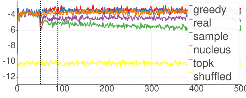
Figure 1: The average log likelihood (y-axis) predicted by RoBERTa at each time step (x-axis). The first dotted line is the averaged length of prefix, and the second one is the averaged $\rho$.

4.4 Significance of Mistakes Prior to Repetitive Loops

We then check how significant the mistakes are to the GPT-2 model. Though the previous sections have shown the existence of the mistakes in the early stage. However, to cause misbehavior, the mistakes must be significant enough to cause GPT-2 to behave differently. Therefore, we check how differently GPT-2 processes the generated text compared to the way it processes the real ones.

4.4.1 Measuring the Significance of Mistakes

To measure the significance of mistakes, we inspect the hidden states of GPT-2 when generating passages. For each layer $l>1$ and time step $t$, the artificial state $h^{(\hat{y})}_{l,t}$ is the result of applying the $\mathrm{transformer}$ function $l-1$ times over the input sequence $\{\hat{y}_{l-1,\tau}\}_{\tau=1...t-1}$, which is the prefix of the artificial passage. Therefore, if a artificial state $h^{(\hat{y})}_{l,t}$ is significantly dissimilar to any real states, then it implies that the generated passage $\{\hat{y}_{l-1,\tau}\}_{\tau=1...t-1}$ contains mistakes that are significant to the model, and that the mistakes do lead the model to an unseen state. Thus, the similarity between the artificial states and the real state indicates how significant the mistakes in the passage are.

Specifically, we measure how many real state is similar to a artificial state. It is done by counting the number of real states in the neighbor of the artificial state. A lower number of real neighborhoods suggests that the artificial state is more unseen, and thus implies higher significance of the mistakes.

Formally, given a hidden state $h_{l,t}^{(\hat{y})}$ at the time step $t$ in the layer $l$, we count the number of real states in a support set $H^{Y}_{l,t}$ which is close to $h_{l,t}^{(\hat{y})}$:

$$N(h_{l,t}^{(\hat{y})})=\left|\left\{\left\lVert h_{l,t}^{(\hat{y})}-h\right\rVert_{2}<r\middle|h\in H^{Y}_{l,t}\right\}\right\rvert$$ (7)

where $r$ is the predefined radius.

We use different $H_{l,t}$ depending on the layer $l$ and the time step $t$ of the hidden state $h_{l,t}^{(\hat{y})}$ to be considered. We compare $h_{l,t}^{(\hat{y})}$ only with the real states of the same layer, $H^{Y}_{l,t}$ only contains state of the same layer. To reduces the required computation power, we also limit the set $H_{l,t}$ to the state of the tokens whose time step differ to $t$ by less than $\delta$. This limitation is reasonable, because we found the position of the states are time-step-dependent. We found this by projecting the real states to their first two principle components with PCA Pearson (1901). As shown in figure 2, states of nearby time steps are clustered together. Formally, the support set of real neighbors is written as

$$H^{Y}_{l,t}=\{h_{l,\tau}^{(y)}\mid\tau\in[t-\delta,t+\delta],y\in Y\}.$$ (8)

Note that the constitution of $H^{Y}_{l,t}$ depends on a set of real passages $Y$. We will discuss the choice of $Y$ in the next section.

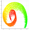
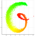
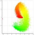
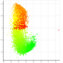
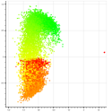
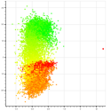
Figure 2: Hidden states projected to their first two principal components. Figures from left to right include states in layers 1, 3, 5, 7, 9, 11. Colors from red to green indicate the time steps from 0 to 512.

4.4.2 Experimental Setting

Roughly speaking, we perform our experiment with two sets of passages $Y_{sup}$ and $Y_{cond}$. We use $Y_{cond}$ to generate real states, and from them we build $H^{Y_{cond}}_{l,t}$ for all layer $l$ and time step $t$. $H^{Y_{cond}}_{l,t}$ can be used to evaluate any state of layer $l$ and $t$. As for $Y_{cond}$, we use it to generate states to be evaluated. By using the prefix of $y\in Y_{cond}$ as condition, we can use it to generate artificial passage $\hat{Y}$ and artificial states. We also generate real states by encoding the whole $y\in Y_{cond}$ with GPT-2. We expect that the states of $y\in Y_{cond}$ to be similar to the states of $y\in Y_{sup}$, while the artificial state $\hat{y}\in\hat{Y}$ to be dissimilar to the artificial ones. Specifically, we conduct the experiment with the following steps:

1. We prepare two disjoint sets of sequences $Y_{cond}$ and $Y_{sup}$. There two sets are parts of the union of the training, validation and testing subsets of WikiText released by OpenAI (as described in Section 4.1).

2. For all $y$ in $Y_{sup}$, we collect a set of real states $h_{sup}$ by using GPT-2 to encode $y$. These real states are used to construct the $H_{l,t}$ as mentioned in 8.

3. For all $y$ in $Y_{cond}$, we generate artificial sequences $\hat{y}$ by conditioning GPT-2 on the first 50 tokens of $y_{cond}\in Y_{cond}$. We experiment with the generation strategies mentioned in Section 3.1. The hidden states $\hat{h}$ are also collected.

4. For all $y$ in $Y_{cond}$, we also use GPT-2 to encode the whole passage $y$ and collect the states $h_{cond}$. Since the sequences $y\in Y_{cond}$ are real, the states $h_{cond}$ are real too.

5. Finally, we evaluate how the states collected with $Y_{cond}$ are similar to the real states from $Y_{real}$. We calculate $N(\hat{h})$, the numbers of artificial states’ real neighbor in $h_{sup}$. We also use $y_{cond}$ calculate $N(h_{cond})$. It is referred to as "real" in Figure 3 and 4.

We prepare $Y_{sup}$ and $Y_{cond}$ in two ways:

compare-seen

The training split is used as $Y_{sup}$. It is seen when training. Real passages in the validation split and the testing split are used as $Y_{cond}$.

compare-unseen

The union of the validation split and the testing split is split into two disjoint subsets by ratio 9:1. They are used as $Y_{sup}$ and $Y_{cond}$ respectively. $Y_{sup}$ is unseen when training.

4.4.3 Sanity Check

We experiment with a set of shuffled states as a sanity check of our approach. It verifies whether the number of neighbors is an indicative measure of the significance of mistakes. The shuffled set is constructed by first shuffling the real passages in the $Y_{cond}$, and is then encoded with GPT-2. The shuffled passages have the same 1-gram distribution as real natural language, but have low likelihood to be real. We expect them to have low numbers of real neighbors.

The results show that the number of real neighbors is a good indication of mistakes for middle layers from layer 5 to layer 9 when $r=1024$ for both the compare-seen and compare-unseen settings. For smaller $r\in{32,64,128,256,512}$, the results are not stable. The average number of neighbors for different time steps at the seventh layer is plot in figure 3. We include the results of other layers in the appendix. The figure shows that the number of neighbors of the shuffled states are consistently low for all time steps. It implies that the number of neighbors is indicative for detecting unreal passages. However, it is less indicative when $R$ is small. We posit that it is due to the high sparsity of the states due to their high dimensionality .

4.4.4 Results

Figure 3 also plots the number of real neighbors ($h$) for states generated with greedy strategy and the sampling-based strategies ($\hat{h}$). For the greedy strategy, the number of neighbors declines rapidly when the time step increases. Note that we observe that repetitive loops occur in about 93% of the sequences. It shows that GPT-2 indeed fails to recover from mistakes, and the mistakes are amplified through time. It is aligned with the description of exposure bias. On the other hand, compared with real sequences (the control group), the number only decreases slightly when sampling-based strategies are used. In contrast to the case of greedy decoding, repetitive loops are rarely observed when those sampling-based methods are used ($<$ 1% for all of the strategies). It implies that if GPT-2 has misbehavior when using those strategies, the misbehavior is less likely to be related to exposure bias.

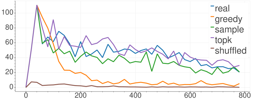
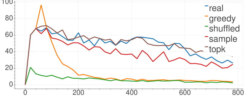
Figure 3: Number of neighbors in the seen-case (top) and unseen-case (bottom) at layer 7. The x-axis is the time step of the tokens. The y-axis is the number of real neighbors with the radius.

We further inspect the number of neighbors of the artificial state prior to the time step $\rho+\lambda$, when a repetitive loop starts. We want to know whether the model does make significant mistakes before $\rho+\lambda$. It is not shown in Figure 3, as it only shows the significance of mistakes in the late stage. To this end, we plot the number of neighbors again in Figure 4. Different from Figure 3, in Figure 4, the $x$-axis is the time step relative to $\rho+\lambda$, so the significance of mistakes before repetitive loops can be manifested. In particular, we compare the number of real neighbors around the real states and the artificial states. Formally, for each artificial passage $\hat{y}$ conditioning on $y_{1,2,\cdots,50}$, we compare the number of neighbors around the state of $n^{(\hat{y})}_{l,t}$, and the state of the real passage following the condition $n^{(y)}_{l,t}$. Here we set the y-axis of Figure 4 to be the difference $(n^{(\hat{y})}_{l,t}-n^{(y)}_{l,t})$.

Surprisingly, in Figure 4, the compare-seen and compare-unseen settings show different trends. At the beginning, the number of neighbors decreases relatively slowly in both of the two settings. At around $x=-10$, the number in both of them drop to less than zero. It indicates that at this time step, some significant mistakes are made. However, the number in the compare-seen setting dramatically grows while the number continues decreasing in the compare-unseen setting. The low number of neighbors in the compare-unseen indicates the low realness of the generated passages. The high number of neighbors in the seen-setting indicates that the model encodes those unreal passages to space close to the states of training data. It may imply that, at this moment, the model fails to generalize, so it incorrectly encodes the unreal passages as seen ones. Finally, the mistakes are amplified. Consequently, the number in both of the settings drops to less than zero. In sum, Figure 4 shows the significance of mistakes made before it starts repeating a looping sequence. Therefore, the second indication of exposure bias is observed.

Table 2: Similarity between the conditioned passage and the generated passage of the same length.

Conditioned Sentences	Similarity (mean/std)
Looping sequences	0.7327 / 0.3226
First sentences	0.2157 / 0.1911
Last sentences	0.1837 / 0.1848

Repeat #	Looping Seq.	First Sent.	Last Sent.
1	0.451 / 0.368	0.148 / 0.155	0.131 / 0.144
2	0.681 / 0.423	0.331 / 0.373	0.337 / 0.377
3	0.888 / 0.282	0.492 / 0.435	0.578 / 0.431

Table 3: The ROUGE-L (mean/std) between the sentences in the generated repetitive loops and $x$, when GPT-2 conditions on the pattern $c,x,\cdots,x$.

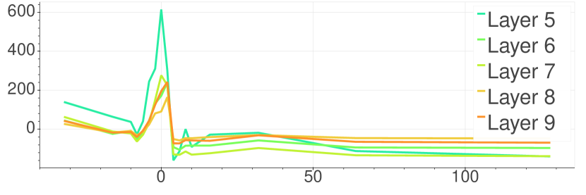
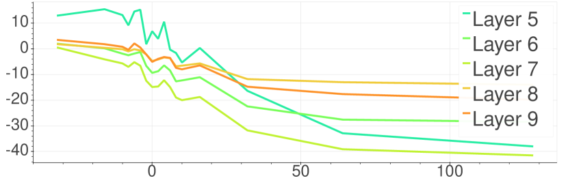
Figure 4: Number of neighbors for setting compare-seen (upper) and compare-unseen (lower). The x-axis is the time step of the tokens relative to $\rho+\lambda$. The y-axis is $(n^{(\hat{y})}_{l,t}-n^{(y)}_{l,t})$.

5 Mechanisms after a Repetitive Loop Starts

While the above experiments show the indications of exposure bias, in this section we further investigate how the early stage mistakes cause the model to degenerate. Figure 4 indicates some mistakes are made prior to time step $\rho+\lambda$. Thus, in this section, we investigate the characteristics of the sequence generated prior to $\rho+\lambda$, the looping sequence $\hat{y}_{\rho}\cdots\hat{y}_{\rho+\lambda}$ (as defined in Section 3.3).

5.1 The Looping Sequence is Loop-Inducing

We investigate how the looping sequences are loop-inducing by using them as conditions when generating text. We construct a looping sequence set that is constituted with all looping sequences generated when conditioning on the first 50 tokens of real sequences. In a generated sequence $\hat{y}$, since $\hat{y}_{\rho}$ may not be a start point of a grammatical sentence, we use the sequence $\hat{y}_{\rho+\delta+1},\cdots,\hat{y}_{\rho+\lambda}\hat{y}_{\rho}\cdots\hat{y}_{\rho+\delta}$, where $\delta$ is chosen based on the punctuation in it . As control groups, we also construct two real sequence sets, first sentence set and last sentence set. They consist of the first sentence and the last sentence of the articles in WikiText validation split and testing split.

To measure how those sequences are looping-inducing, we calculate the similarity between $x$ and $\hat{y}$, where $x$ is the sequence used as condition, and $\hat{y}$ is the generated passage. Specifically, we measure ROUGE-L Lin (2004) between $x$ and the first $\mathrm{length}(x)$ tokens of $\hat{y}$. A higher score implies higher similarity, and thus more looping-inducing. Results shown in Table 2 indicate that looping sequences are indeed more loop-inducing.

5.2 Any Repeating Sequence is Loop-Inducing

We further discover that any sequence that is repeated is loop-inducing, regardless of contexts. We create the conditioned sequence by concatenating $c$ with $x$ repeated from 1 to 3 times, where $c$ is the first 5 sentences from a random article of WebText, and $x$ is either from the looping sequence set or the real sets. Measurement, the same as in Section 5.1 is applied on $x$ and the generated passages. The results are shown in Table 3, and it shows that even when the conditioned sequence is real, it is more loop-inducing if it is repeated more times.

5.3 The Self-Reinforcing Mechanism of Text Degeneration

In sum, in this section, we discover the self-reinforcing mechanism of text degeneration. First, Section 5.1 a looping sequence is loop-inducing. Thus, after a looping sequence is generated, it is likely to be repeated. Second, Section 5.2 shows that when a sequence is repeated, then GPT-2 would be more likely to continue repeating it. Therefore, it shows how GPT-2 fails to recover from the mistake.

6 Conclusion

In conclusion, we provide a deeper insight into the relation between exposure bias and text degeneration. We qualitatively and quantitatively show that mistakes are indeed made in the early stage of generation. In Particular, some significant mistakes are made prior to $\rho+\lambda$, the time step when the model starts repeating. We then show why the model fails to recover from the mistakes. The looping sequence, which is the sequence generated prior to $\rho+\lambda$, and repeated sequences are looping-inducing. That is how the model fails to recover from the mistakes, and how the mistakes amplify.

Our contributions are four-fold: 1) We explicitly formulate the necessary indications for the detection of exposure bias. 2) For each condition, we design the associated experiments for validation. 3) By the experiments, we show that text degeneration is likely to be partly caused by exposure bias. 4) Finally, we provide a possible explanation how GPT-2 fails to recover from the mistake. Our formulation and the conducted experiments build a solid foundation for future study on exposure bias.

Appendix A Sample-based Decoding Strategies

• Sampling: $\hat{y}_{t}$ is directly sampled from the conditional probability $P_{M}(\hat{y}_{t}\mid\hat{y}_{1},\hat{y}_{2},\cdots,\hat{y}_{t-1})$.

• Top-$k$ sampling Fan et al. (2018): At the time step $t$, $\hat{y}_{t}$ is sampled from the conditional probability:

  $${P}_{Y}(\hat{y}_{t}\mid\hat{y}_{1},\hat{y}_{2},\cdots,\hat{y}_{t-1})\propto$$

  $$\begin{cases}P_{M}(\hat{y}_{t}\mid\hat{y}_{1},\hat{y}_{2},\cdots,\hat{y}_{t-1})&\text{if $\hat{y}_{t}\in$ top-$k$,}\\ 0&\text{otherwise.}\end{cases}$$ (9)

• Nucleus sampling Holtzman et al. (2020): At the time step $t$, $\hat{y}_{t}$ is sampled from the conditional probability

  $${P}_{Y}(\hat{y}_{t}\mid\hat{y}_{1},\hat{y}_{2},\cdots,\hat{y}_{t-1})\propto$$

  $$\begin{cases}P_{M}(\hat{y}_{t}\mid\hat{y}_{1},\hat{y}_{2},\cdots,\hat{y}_{t-1})&\text{if $\hat{y}_{t}\in V^{(p)}$}\\ 0&\text{otherwise.}\end{cases},$$ (10)

  and for a predefined $p\in(0,1]$, $V^{(p)}$ is the minimal set that satisfies

  $$\sum_{v\in V^{(p)}}P_{M}(v\mid\hat{y}_{1},\hat{y}_{2},\cdots,\hat{y}_{t-1})\geq p$$ (11)

Appendix B Dataset

We use the subsets of WebText released by OpenAI (https://github.com/openai/gpt-2-output-dataset). It is an English dataset. There are 25000, 5000, 5000 passages in the train, validation, testing splits respectively. For experiments in Section 4.3 and Section 4.4), we only use the passages with more than 512 tokens. After passages with less than 512 tokens are removed, there are 5269 passages in the union of the validation split and the testing split.

Appendix C Detail of Experiments

C.1 Quantitative Inspection of Generated Tokens Priors to Repetitive Loops (Section 4.3)

Implementation of RoBERTa from Python package transformers 2.8.0 by Hugging Face (https://huggingface.co/transformers/) is used.

C.2 Significance of Mistakes Prior to Repetitive Loops (Section 4.4)

We use Faiss Johnson et al. (2017) to calculate the number of neighbor vectors within a radius. For Figure 3, the number of neighbors is calculated for 20 time steps. For Figure 4, the number of neighbors is calculated at time steps {-32, -16, -10, -8, -6, -4, -2, 0, 2, 4, 6, 8, 10, 16, 32, 64, 128} relative to $\rho+\lambda$.

Seen-setting:

We sampled 2500 passages from the WebText training split. Each line in Figure 4 is the average over 500 passages generated by each decoding strategy. The result in Figure 4 is the average over 1000 passages.

Unseen-setting:

We first combine the validation split and the testing split as the set of all real unseen text $\bar{Y}$. Then we split it into 10 equal-sized subsets $\bar{Y}_{1},\bar{Y}_{2},\cdots,\bar{Y}_{10}$. We repeat the following process 3 times:

• From $\{\bar{Y}_{1},\bar{Y}_{2},\cdots,\bar{Y}_{10}\}$, a subset $Y_{real}$ is selected, and the rest $\bar{Y}\textbackslash Y_{real}$ is used as the support set $Y_{support}$.

• Real states are collected by encoding passages in $Y_{support}$ with GPT-2. When we are calculating the number of neighbors, only these real states are counted.

• Artificial passages are generated by conditioning on the first 50 tokens for passages in $Y_{real}$ using the decoding strategies.

• The number of neighbors is calculated for each decoding strategies.

Finally, the result is averaged to plot Figure 3 and Figure 4.

C.3 Automatic Detection of Looping Sequence

Given a passage $x_{1},x_{2},\cdots,x_{T}$, we first search for the length of a repetitive loop by comparing $x_{T-\lambda+1},\cdots x_{T}$ and $x_{T-2\lambda+1},\cdots x_{T-\lambda}$ for $\lambda=4,5,\cdots,l/2,1,2,3$. If there exists some $\lambda$ such that $x_{T-\lambda+1},\cdots,x_{T}=x_{T-2\lambda+1},\cdots,x_{T-\lambda}$, then we search $\rho$ as the first place such that $x_{\rho+i\lambda},\cdots,x_{\rho+(i+1)\lambda-1}=x_{T-2\lambda+1+\delta},\cdots,x_{T-\lambda+\delta}$ for some $\delta\in[0,\lambda-1]$ and all $i$ such that $\rho+i\lambda<T$.

Appendix D Computing Infrastructure

Each of our experiments were run on a workstation with 187 GiB RAM. A workstation is equipped with either two Intel Xeon 5218 CPUs or two Intel Xeon 4110 CPUs. Every experiment can be run with 1 Nvidia GTX 2080Ti GPU.

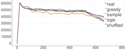
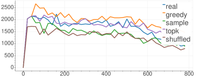
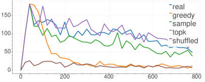
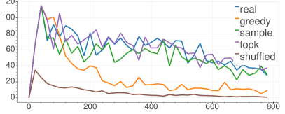
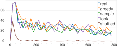
Figure 5: Number of neighbors for compare-seen setting. The figures are the number of layer 1, 3, 5, 7, 9, 11, from left to right, top to bottom. The x-axis is the time step of the tokens. The y-axis is the number of real neighbors with the radius.

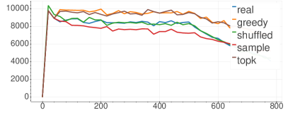
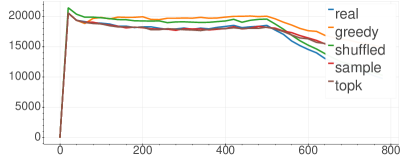
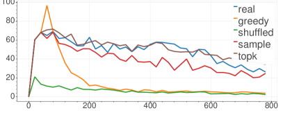
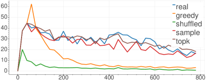
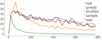
Figure 6: Number of neighbors for compare-unseen setting. The figures are the number of layers 1, 3, 5, 7, 9, 11, from left to right, top to bottom. The x-axis is the time step of the tokens. The y-axis is the number of real neighbors with the radius.

References

- Bengio et al. (2015) Samy Bengio, Oriol Vinyals, Navdeep Jaitly, and Noam Shazeer. 2015. Scheduled sampling for sequence prediction with recurrent neural networks. In Advances in Neural Information Processing Systems, pages 1171–1179.
- Daumé et al. (2009) Hal Daumé, John Langford, and Daniel Marcu. 2009. Search-based structured prediction. Machine learning, 75(3):297–325.
- Fan et al. (2018) Angela Fan, Mike Lewis, and Yann Dauphin. 2018. Hierarchical neural story generation. arXiv preprint arXiv:1805.04833.
- He et al. (2019) Tianxing He, Jingzhao Zhang, Zhiming Zhou, and James Glass. 2019. Quantifying exposure bias for neural language generation. arXiv preprint arXiv:1905.10617.
- Holtzman et al. (2020) Ari Holtzman, Jan Buys, Li Du, Maxwell Forbes, and Yejin Choi. 2020. The curious case of neural text degeneration. In International Conference on Learning Representations.
- Huszár (2015) Ferenc Huszár. 2015. How (not) to train your generative model: Scheduled sampling, likelihood, adversary? arXiv preprint arXiv:1511.05101.
- Johnson et al. (2017) Jeff Johnson, Matthijs Douze, and Hervé Jégou. 2017. Billion-scale similarity search with gpus. arXiv preprint arXiv:1702.08734.
- Lamb et al. (2016) Alex M Lamb, Anirudh Goyal Alias Parth Goyal, Ying Zhang, Saizheng Zhang, Aaron C Courville, and Yoshua Bengio. 2016. Professor forcing: A new algorithm for training recurrent networks. In Advances In Neural Information Processing Systems, pages 4601–4609.
- Li et al. (2019) Margaret Li, Stephen Roller, Ilia Kulikov, Sean Welleck, Y-Lan Boureau, Kyunghyun Cho, and Jason Weston. 2019. Don’t say that! making inconsistent dialogue unlikely with unlikelihood training. arXiv preprint arXiv:1911.03860.
- Lin (2004) Chin-Yew Lin. 2004. ROUGE: A package for automatic evaluation of summaries. In Text Summarization Branches Out, pages 74–81, Barcelona, Spain. Association for Computational Linguistics.
- Liu et al. (2019) Yinhan Liu, Myle Ott, Naman Goyal, Jingfei Du, Mandar Joshi, Danqi Chen, Omer Levy, Mike Lewis, Luke Zettlemoyer, and Veselin Stoyanov. 2019. Roberta: A robustly optimized bert pretraining approach. arXiv preprint arXiv:1907.11692.
- Muller et al. (2006) Urs Muller, Jan Ben, Eric Cosatto, Beat Flepp, and Yann L Cun. 2006. Off-road obstacle avoidance through end-to-end learning. In Advances in neural information processing systems, pages 739–746.
- Pearson (1901) Karl Pearson. 1901. Liii. on lines and planes of closest fit to systems of points in space. The London, Edinburgh, and Dublin Philosophical Magazine and Journal of Science, 2(11):559–572.
- Petroni et al. (2019) Fabio Petroni, Tim Rocktäschel, Sebastian Riedel, Patrick Lewis, Anton Bakhtin, Yuxiang Wu, and Alexander Miller. 2019. Language models as knowledge bases? In Proceedings of the 2019 Conference on Empirical Methods in Natural Language Processing and the 9th International Joint Conference on Natural Language Processing (EMNLP-IJCNLP), pages 2463–2473, Hong Kong, China. Association for Computational Linguistics.
- Pomerleau (1989) Dean A Pomerleau. 1989. Alvinn: An autonomous land vehicle in a neural network. In Advances in neural information processing systems, pages 305–313.
- Radford (2018) Alec Radford. 2018. Improving language understanding by generative pre-training.
- (17) Alec Radford, Jeffrey Wu, Rewon Child, David Luan, Dario Amodei, and Ilya Sutskever. Language models are unsupervised multitask learners.
- Ranzato et al. (2016) Marc’Aurelio Ranzato, Sumit Chopra, Michael Auli, and Wojciech Zaremba. 2016. Sequence level training with recurrent neural networks. In 4th International Conference on Learning Representations, ICLR 2016, San Juan, Puerto Rico, May 2-4, 2016, Conference Track Proceedings.
- Ratliff et al. (2006) Nathan D Ratliff, J Andrew Bagnell, and Martin A Zinkevich. 2006. Maximum margin planning. In Proceedings of the 23rd international conference on Machine learning, pages 729–736.
- Ross and Bagnell (2010) Stéphane Ross and Drew Bagnell. 2010. Efficient reductions for imitation learning. In Proceedings of the thirteenth international conference on artificial intelligence and statistics, pages 661–668.
- Ross et al. (2011) Stéphane Ross, Geoffrey Gordon, and Drew Bagnell. 2011. A reduction of imitation learning and structured prediction to no-regret online learning. In Proceedings of the fourteenth international conference on artificial intelligence and statistics, pages 627–635.
- Schaal (1999) Stefan Schaal. 1999. Is imitation learning the route to humanoid robots? Trends in cognitive sciences, 3(6):233–242.
- Schmidt (2019) Florian Schmidt. 2019. Generalization in generation: A closer look at exposure bias. In Proceedings of the 3rd Workshop on Neural Generation and Translation, pages 157–167, Hong Kong. Association for Computational Linguistics.
- See et al. (2019) Abigail See, Aneesh Pappu, Rohun Saxena, Akhila Yerukola, and Christopher D. Manning. 2019. Do massively pretrained language models make better storytellers? In Proceedings of the 23rd Conference on Computational Natural Language Learning (CoNLL), pages 843–861, Hong Kong, China. Association for Computational Linguistics.
- Strobelt et al. (2018) Hendrik Strobelt, Sebastian Gehrmann, Michael Behrisch, Adam Perer, Hanspeter Pfister, and Alexander M Rush. 2018. Seq2seq-vis: A visual debugging tool for sequence-to-sequence models. IEEE transactions on visualization and computer graphics, 25(1):353–363.
- Talmor et al. (2019) Alon Talmor, Jonathan Herzig, Nicholas Lourie, and Jonathan Berant. 2019. CommonsenseQA: A question answering challenge targeting commonsense knowledge. In Proceedings of the 2019 Conference of the North American Chapter of the Association for Computational Linguistics: Human Language Technologies, Volume 1 (Long and Short Papers), pages 4149–4158, Minneapolis, Minnesota. Association for Computational Linguistics.
- Thrun (1995) Sebastian Thrun. 1995. Learning to play the game of chess. In Advances in neural information processing systems, pages 1069–1076.
- Vaswani et al. (2017) Ashish Vaswani, Noam Shazeer, Niki Parmar, Jakob Uszkoreit, Llion Jones, Aidan N Gomez, Łukasz Kaiser, and Illia Polosukhin. 2017. Attention is all you need. In Advances in neural information processing systems, pages 5998–6008.
- Wang and Sennrich (2020) Chaojun Wang and Rico Sennrich. 2020. On exposure bias, hallucination and domain shift in neural machine translation. In Proceedings of the 58th Annual Meeting of the Association for Computational Linguistics, pages 3544–3552, Online. Association for Computational Linguistics.
- Welleck et al. (2020) Sean Welleck, Ilia Kulikov, Stephen Roller, Emily Dinan, Kyunghyun Cho, and Jason Weston. 2020. Neural text generation with unlikelihood training. In International Conference on Learning Representations.
- Wiseman and Rush (2016) Sam Wiseman and Alexander M. Rush. 2016. Sequence-to-sequence learning as beam-search optimization. In Proceedings of the 2016 Conference on Empirical Methods in Natural Language Processing, pages 1296–1306, Austin, Texas. Association for Computational Linguistics.
- Yu et al. (2017) Lantao Yu, Weinan Zhang, Jun Wang, and Yong Yu. 2017. Seqgan: Sequence generative adversarial nets with policy gradient. In Thirty-First AAAI Conference on Artificial Intelligence.
- Zhang et al. (2019a) Wen Zhang, Yang Feng, Fandong Meng, Di You, and Qun Liu. 2019a. Bridging the gap between training and inference for neural machine translation. In Proceedings of the 57th Annual Meeting of the Association for Computational Linguistics, pages 4334–4343, Florence, Italy. Association for Computational Linguistics.
- Zhang et al. (2019b) Yizhe Zhang, Siqi Sun, Michel Galley, Yen-Chun Chen, Chris Brockett, Xiang Gao, Jianfeng Gao, Jingjing Liu, and Bill Dolan. 2019b. Dialogpt: Large-scale generative pre-training for conversational response generation. arXiv preprint arXiv:1911.00536.