Superluminous supernovae: an explosive decade

Abstract

I review our current understanding of superluminous supernovae, mysterious events 100 times brighter than conventional stellar explosions.

1 Introduction: the discovery of SLSNe

The study of supernovae spans centuries and cultures, with Chinese astronomers recording the oldest known ‘guest star’ in 185 AD. By the turn of the millenium, it was well established that core-collapse supernovae (CCSNe) signal the death of a star of more than 8 M_⊙ (where M_⊙ is the solar mass). When the nuclear reactor in its core has converted all its fuel into stable iron, and can no longer extract energy to support itself, it collapses to a neutron star and releases its gravitational energy. Type Ia supernovae (SNe Ia) occur when a white dwarf gains sufficient mass from a binary companion to encounter a runaway thermonuclear reaction. Both types of supernova release $\sim 10^{51}$ erg in kinetic energy, peak with a luminosity up to $10^{9}$ L_⊙, and produce many of the chemical elements needed for life in the Universe.

A more extreme class of ‘superluminous supernovae’ (SLSNe), $\sim 10-100$ times brighter again, escaped our notice until the 21st century. Their eventual discovery was intimately tied with advances in optical sky surveys in the mid-to-late 2000s. Figure 1 shows the growth in the supernova discovery rate from 1996-2020, with a sharp uptick around 2010 driven by wide-field robotic telescopes and automated source detection employed by surveys such as the Catalina Real-time Transient Survey (CRTS; Drake et al., 2009), the Panoramic Survey Telescope and Rapid Reponse System (PanSTARRS; Kaiser et al., 2010) and the Palomar Transient Factory (PTF; Rau et al., 2009). Nearly 20,000 supernovae were reported in 2020 – a 100-fold increase in just 20 years. The volumetric rate of SLSNe is only $\sim$1 in every few thousand supernovae (Quimby et al., 2013; Frohmaier et al., 2021), though because these brighter explosions can be detected out to greater distances, they should make up $\sim$1% of the supernovae detected by a given survey. Finding SLSNe in significant numbers therefore requires the discovery and classification of hundreds or thousands of supernovae per year.

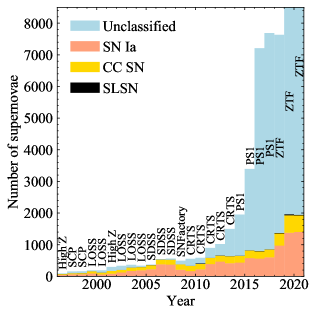
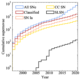
Figure 1: Supernova detection rates and the discovery of SLSNe. Data have been obtained from the Latest Supernova Page, the Open Supernova Catalog and the Transient Name Server. Left: Stacked histogram showing supernova discoveries per year, labelled with the survey that detected the majority. The 2010s show a sharp rise driven by robotic surveys. Most events now go unclassified due to finite telescope time. Middle: Cumulative supernova counts. Several thousand core collapse and Type Ia SNe, and over 100 SLSNe, have now been classified. Right: SLSN detection efficiency, defined as the fraction of SLSNe out of all classified supernovae each year, compared to the fraction expected given their estimated occurrence rate (the shaded region shows the uncertainty on their true rate; Frohmaier et al. 2021). The efficiency rose dramatically when wide-field surveys removed the bias towards massive galaxies.

Yet Figure 1 also shows that the fraction (not just the absolute number) of SLSNe within a given survey also increased dramatically in 2010. Earlier surveys had targeted massive galaxies that have a correspondingly high rate of CCSNe and SNe Ia, but it turns out that SLSNe exhibit a strong and surprising predilection for dwarf galaxies (section 4.3). Therefore the unbiased nature of modern surveys – observing wide areas rather than specific galaxies – was also key to their discovery. While the first reported SLSNe – SN2005ap (Quimby et al., 2007), SN2006gy (Smith et al., 2007; Ofek et al., 2007), SN2007bi (Gal-Yam et al., 2009; Young et al., 2010) – were all major discoveries, the birth of SLSNe as a full-fledged field of study can arguably be traced to 2011. Quimby et al. (2011) presented five SLSNe from PTF, and showed that they formed a class with similar properties to SN2005ap (and the previously mysterious high-redshift transient SCP06F6 Barbary et al. 2009). In the same year, Chomiuk et al. (2011) published the first two SLSNe from PanSTARRS. Since then, our knowledge of SLSNe and our ability to spot new candidates have grown hand-in-hand, and we now have a sample of $\sim 100$ such events – growing rapidly thanks to current surveys like the Zwicky Transient Facility (Bellm et al., 2019; Lunnan et al., 2020), ATLAS (Tonry et al., 2018), Gaia (Hodgkin et al., 2021) and ASASSN (Shappee et al., 2014).

Here I review the progress we have made in characterising and understanding SLSNe over the past decade, and look ahead to a bright future. The interested reader can find further reviews by Howell (2017), Moriya et al. (2018a), Inserra (2019), Gal-Yam (2019a) and Chen (2021).

2 Observed and defining properties

Gal-Yam (2012) initially separated SLSNe from other supernova types with a simple threshold in optical absolute magnitude: $M<-21$ mag, or a luminosity

$$L_{\rm peak}\gtrsim 10^{10}\,{\rm L}_{\odot}\approx 3\times 10^{43}\,{\rm erg}\,{\rm s}^{-1}.$$ (1)

This is around 10 times brighter than a SN Ia or 100 times brighter than a CCSN (Figure 2). The time taken to reach peak luminosity is also longer for SLSNe, with exponential rise timescales $\sim 15-50$ days (Nicholl et al., 2015a). Integrating the high luminosity over the broad light curve gives a total radiative energy $\sim 10^{51}$ erg, 1000 times that of a normal CCSN and comparable to their total kinetic energy.

As with traditional supernovae, SLSNe have been partitioned into two sub-types: with (SLSNe II) and without (SLSNe I) hydrogen lines in the spectrum. Physically, the distinction is whether the star retained a hydrogen envelope until the point of explosion, or was stripped by e.g. stellar winds or binary interaction. SLSNe II usually show hydrogen emission lines with narrow Doppler widths, indicating low-velocity circumstellar material (CSM) that has been shock-excited by a collision from the supernova ejecta (e.g. Smith et al. 2007; Drake et al. 2010; Chatzopoulos et al. 2011; Benetti et al. 2014; but see Miller et al. 2009; Gezari et al. 2009; Inserra et al. 2018a for examples with broad lines). These seem to be differentiated from less luminous Type ‘IIn’ (for narrow-lined) SNe primarily by the radius/density/mass of the CSM, though the extremes of this population require a kinetic energy in the supernova ejecta well in excess of the usual $10^{51}$ erg (Rest et al., 2011; Nicholl et al., 2020).

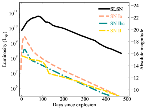
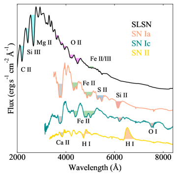
Figure 2: Basic properties of SLSNe compared to SNe Ia and hydrogen-rich (SNe II) and -poor (SNe Ib/c) CCSNe. Left: The broad, luminous light curves of SLSNe release $\sim 1000$ times more energy than conventional CCSNe. Right: SLSNe are defined by a blue spectrum at the time of peak luminosity, with absorption lines of singly-ionized oxygen. SLSNe show stronger lines in the UV, but still radiate significantly more UV flux than other supernova types.

Hydrogen-poor SLSNe I, on the other hand, have a unique spectrum at the time of their peak luminosity (Figure 2), with a steep blue continuum and a series of broad absorption lines that Quimby et al. (2011) identified as singly-ionized oxygen (O II). The optical range may also include weak lines of Si II (Inserra et al., 2013), Fe III (Leloudas et al., 2012; Nicholl et al., 2013) and C II (Nicholl et al., 2016b; Anderson et al., 2018). The ultraviolet range is more line-rich, showing deep absorptions from Mg II, C II, Si III and Fe III (Quimby et al., 2011; Vreeswijk et al., 2014; Yan et al., 2017a, 2018; Quimby et al., 2018). Rather than using a hard magnitude cut, the term SLSN (often used interchangeably with SLSN I) is now typically applied to any event exhibiting this distinctive spectrum, and in fact the range of observed SLSN peak magnitudes now extends at least a magnitude fainter than the original $-21$ mag (Quimby et al., 2018; De Cia et al., 2018; Lunnan et al., 2018a; Angus et al., 2019). There is a continuing debate in the literature as to whether SLSNe I separate further into a class of slowly-evolving events with lower velocities and cooler temperatures, and faster-evolving events with higher velocities and temperatures (Quimby et al., 2018; Inserra et al., 2018b). Recently, helium has also been identified in the spectra of up to $\sim 10$% of SLSNe (Quimby et al., 2018; Yan et al., 2020), suggesting another possible sub-division into SLSNe Ib (stripped of hydrogen) and Ic (stripped of hydrogen and helium), in analogy with ordinary SNe Ib and Ic.

In fact, the relationship between SLSNe and normal stripped-envelope CCSNe is more than analogous. Pastorello et al. (2010) observed that around a month after peak luminosity, the spectrum of a SLSN closely resembles SNe Ic, including the broad-lined SNe Ic that accompany long-duration gamma-ray bursts (long GRBs). This has been confirmed in many studies since, for both fast and slowly evolving SLSNe (e.g. Inserra et al., 2013; Nicholl et al., 2013; Blanchard et al., 2019). This convergence shows the importance of temperature in determining which atomic lines are excited. SLSNe remain hotter for longer than normal SNe Ic, with $T\gtrsim 12000-15000$ K at maximum light (Figure 3). That SLSNe resemble normal SNe Ic once they have cooled to $\sim 8000$ K suggests a similar elemental composition in their ejecta: primarily intermediate mass elements such as oxygen, carbon, magnesium and silicon, with some iron-group elements. For this reason I suggest that a better way to think of SLSNe is as ‘ultra-hot’ SNe Ic. The higher temperature at maximum light not only explains the unusual blue spectrum, but accounts for the higher luminosity via Stefan’s law of blackbody emission: $L=4\pi R^{2}\sigma T^{4}$, where $R\sim 10^{15}$ cm is the radius of the emitting surface and $\sigma$ the Stefan-Boltzmann constant. Our goal in explaining the luminosity of SLSNe is thus to uncover this heating source.

3 Physical mechanisms for SLSNe

The basic properties of a supernova can be understood using “Arnett’s Rule” (Arnett, 1982). At the peak of the light curve, the luminosity is equal to the heating rate: $L_{\rm peak}=\dot{E}(t=t_{\rm peak})$. The peak occurs roughly on the photon diffusion timescale,

$$t_{\rm peak}\sim t_{\rm diff}=\left(\frac{3\kappa M_{\rm ej}}{4\pi cv_{\rm ej}}\right)^{1/2},$$ (2)

where $c$ is the speed of light. The velocity of the ejecta, $v_{\rm ej}\approx 10^{4}$ km s^-1, can be measured from Doppler shifts and broadening of spectral lines. The opacity, $\kappa\approx 0.1$ cm² g^-1, is dominated by scattering from free electrons in the ionised ejecta. Finally, $M_{\rm ej}$ is the mass of the supernova ejecta, corresponding to the final mass of the (stripped) star minus the mass of the compact remnant (neutron star or black hole) left behind. Observed SLSN peak times imply a broad range of ejected masses, from a few up to a few tens of solar masses (Inserra et al., 2013; Nicholl et al., 2015a; Nicholl et al., 2017c; Lunnan et al., 2016; Blanchard et al., 2020).

Three candidate power sources have emerged to explain the long-term heating in SLSNe, outlined below. Example light curves from these models are shown in Figure 4.

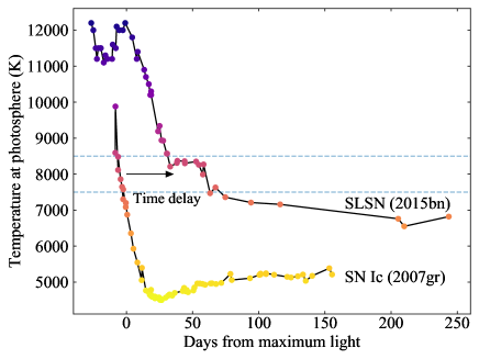
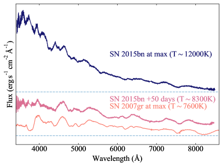
Figure 3: The link between SLSNe and normal stripped-envelope SNe Ic. Left: Temperature evolution. SLSNe are hotter at peak and take longer to cool than SNe Ic. Right: Observed spectra, coloured using the temperature scale from the left panel. Although the spectra of SLSNe and SNe Ic are quite distinct at the time of maximum light, they look remarkably similar when grouped by temperature rather than light curve phase. Data are from Valenti et al. (2008); Nicholl et al. (2016a).

3.1 Radioactive decay

Normal hydrogen-poor supernovae are powered by radioactive ⁵⁶Ni, a product of explosive nucleosynthesis, providing an energy

$$\dot{E}_{\rm Ni}\sim 10^{43}\ (M_{\rm Ni}/{\rm M}_{\odot})\ \left(6.5\exp{\left(-t/\tau_{\rm Ni}\right)}+1.5\exp{\left(-t/\tau_{\rm Co}\right)}\right)\ {\rm erg}\,{\rm s}^{-1},$$ (3)

where $M_{\rm Ni}$ is the mass of nickel, decaying with lifetime $\tau_{\rm Ni}=8.8$ days to ⁵⁶Co, which in turn decays with lifetime $\tau_{\rm Co}=111.3$ days to stable ⁵⁶Fe (Nadyozhin, 1994). SNe Ic produce $M_{\rm Ni}\lesssim 0.1$ M_⊙ (Drout et al., 2011; Prentice et al., 2019); SNe Ia produce $M_{\rm Ni}\lesssim 0.5$ M_⊙ (e.g. Childress et al., 2015). To power a SLSN with $L_{\rm peak}\sim 10^{44}$ erg s^-1 at $t_{\rm peak}\sim 30$ days would need an enormous $M_{\rm Ni}\gtrsim 7$ M_⊙. This could theoretically be produced by a ‘pair-instability’ supernova from a carbon-oxygen core of over 100 M_⊙ (Barkat et al., 1967; Heger & Woosley, 2002).

However, this 100 M_⊙ ejecta would be inconsistent with the observed rise timescales of nearly all SLSNe (Kasen et al., 2011; Dessart et al., 2013; Kozyreva & Blinnikov, 2015). Including the requisite nickel mass in a lower mass ejecta would need $M_{\rm Ni}/M_{\rm ej}\sim 1$. Yet the observed spectra of even the most slowly evolving (high mass) SLSNe show primarily carbon-oxygen ejecta, rather than enhanced iron-group absorption (Dessart et al., 2012; Nicholl et al., 2013). Finally, observed upper limits on ⁵⁶Co luminosity at $\sim 100$ days after explosion are inconsistent with the much larger ⁵⁶Ni mass needed to power the peak (Inserra et al., 2013; Blanchard et al., 2018). For these reasons, the radioactive model is disfavoured for (at least) the vast majority of SLSNe.

3.2 Central engine

A more successful model for explaining SLSNe is a ‘central engine’, with the most obvious candidate being rotation of the newborn neutron star formed during core collapse. Neutron stars have a radius $\sim 12$ km, giving a minimum spin period $\sim 1$ ms or a maximum rotational energy $\sim 10^{52}$ erg (for a typical mass of $1.4$ M_⊙). If the spin and magnetic axes are mis-aligned, this energy is extracted by magnetic dipole emission (Ostriker & Gunn, 1971; Kasen & Bildsten, 2010; Woosley, 2010):

$$\dot{E}_{\rm mag}\sim 2\times 10^{47}\ (B/10^{14}{\rm G})^{2}\ (P/{\rm ms})^{-4}\ (1+t/\tau_{\rm mag})^{-2}\ {\rm erg}\,{\rm s}^{-1},$$ (4)

for initial spin period $P$ in seconds and magnetic field $B$ in Gauss, and a spin-down timescale $\tau_{\rm mag}\approx{\rm 1~{}day}\ (P/{\rm ms})^{2}\ (B/10^{14}{\rm G})^{-2}$. Although the energy available from a millisecond rotator exceeds that in a typical supernova, it can only alter the peak luminosity if it spins down in days or weeks, rather than years or longer. The maximum $L_{\rm peak}\sim 10^{45}$ erg s^-1 occurs for $\tau_{\rm mag}\sim t_{\rm peak}$, which requires $B\sim 10^{13-14}$ G.

Observed Galactic neutron stars with $B\gtrsim 10^{14}$ G, known as ‘magnetars’, demonstrate that such field strengths are feasible (Thompson & Duncan, 1996). Although known magnetars currently rotate with $P_{\rm now}\gg 1$ ms, their spins may have been much faster at birth. Conservation of angular momentum suggests that many neutron stars should be born rapidly rotating. SLSNe would therefore occur for the fraction of neutron stars that are also born with the right magnetic field.

An alternative central engine utilizes black holes rather than neutron stars. In this scenario, fallback accretion onto the black hole could liberate gravitational energy to power the explosion (Dexter & Kasen, 2013). However, the long durations of SLSNe require fallback timescales more consistent with extended envelopes than with compact carbon-oxygen cores. Furthermore, systematic comparison of this model with observed SLSNe suggests that (for a reasonable conversion efficiency of mass to energy) an unrealistic fallback mass of tens or hundreds of solar masses would be required (Moriya et al., 2018b).

3.3 Circumstellar interaction

The final class of models for powering SLSNe is via interaction with a dense CSM, produced by pre-explosion mass-loss from the progenitor. This offers at least three ways to generate a luminous light curve: shock breakout inside an extended wind (Chevalier & Irwin, 2011); diffusion from a shock-heated CSM shell (Smith & McCray, 2007); and continuous conversion of kinetic to thermal energy as ejecta collide with slower material (Ginzburg & Balberg, 2012; Chatzopoulos et al., 2012). In all cases, the relevant energy scale is $\epsilon E_{\rm k}$, with kinetic energy $E_{\rm k}\approx 10^{51}$ erg and an efficiency factor $\epsilon$, close to unity in SLSNe, for converting this to light. An inelastic collision removes a fraction $\epsilon=M_{\rm CSM}/(M_{\rm ej}+M_{\rm CSM})$ of the ejecta kinetic energy, and hence the condition for powering a SLSN is a CSM mass $M_{\rm CSM}\gtrsim M_{\rm ej}$. This can also be seen via the peak luminosity,

$$L_{\rm peak,CSM}\sim 1/2\ M_{\rm CSM}v_{\rm ej}^{2}/t_{\rm peak};$$ (5)

SLSNe are possible for $M_{\rm CSM}\gtrsim 1$ M_⊙. The ejecta must catch up to the CSM before $t_{\rm peak}$, placing it at a maximum distance of $\sim 10^{15}$ cm. This is consistent with the observed blackbody radii of SLSNe at peak.

The ejecta-CSM interaction model is appealing for a number of reasons. Interaction is seen to varying degrees in many normal supernovae – exciting narrow lines in the spectra of SNe IIn (Schlegel, 1990) and producing X-ray and radio emission in both SNe II and SNe Ib/c (Chevalier & Fransson, 1994; Weiler et al., 2002; Berger et al., 2003) – and probably powers hydrogen-rich Type II SLSNe. Moreover, the progenitors of hydrogen-poor SLSNe have lost their outer layers prior to explosion, providing a natural source of CSM.

However, the radius of the CSM at the time of explosion suggests it was ejected only in the last few years–decades, requiring mass-loss rates $\gtrsim 0.1$ M_⊙ yr^-1. This is orders of magnitude greater than the densest stellar winds from Wolf-Rayet stars (Crowther, 2007). The envelope could instead be lost through binary interactions late in the progenitor evolution, or major outbursts: perhaps something akin to the eruptions of luminous blue variable (LBV) stars and/or Eta Carinae, or the predicted ‘pulsational pair-instability’ oscillations of stars with core masses in the range $35-65$ M_⊙ (Woosley et al., 2007; Woosley, 2017).

Given their successes in explaining the luminosities and timescales of SLSNe, most studies now focus on central engines and/or circumstellar interaction as the primary energy source(s). However, it remains possible that some other, currently unknown mechanism may turn out to be the key to producing SLSNe. In the next section, I will review how we use other clues to understand the progenitors and explosion mechanisms of SLSNe.

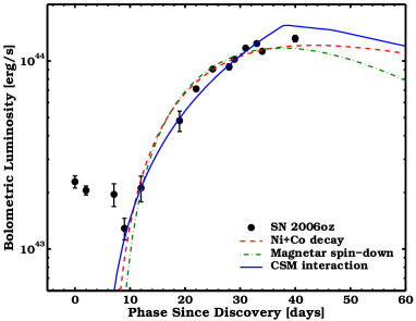
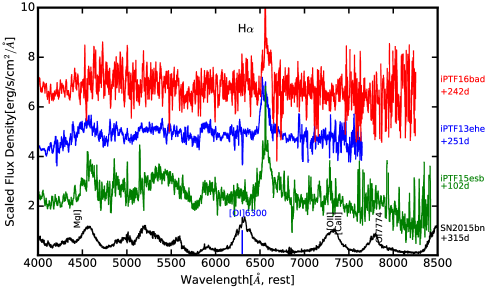
Figure 4: Left, from Leloudas et al. (2012): Light curve of SLSN 2006oz. Radioactive decay, magnetar spin-down, and circumstellar interaction can all fit the peak luminosity, but the radioactive model requires an unrealistic fraction of ⁵⁶Ni in the ejecta. The light curve shows an early ‘bump’, not naturally accommodated by any simple model. Right, from Yan et al. (2017b): Hydrogen Balmer (H$\alpha$) emission lines have appeared suddenly in the spectra of three previously H-poor SLSNe, indicating the ejecta have caught up with a hydrogen envelope lost by the progenitor only decades prior to explosion.

4 Observational clues to the nature of SLSNe

4.1 Spectroscopy and velocity evolution

Spectral lines in supernovae are formed by atomic transitions in cooler outer layers, absorbing and scattering blackbody photons emitted from the photosphere (the surface where the optical depth to free electron-scattering is unity). The lines are Doppler-broadened by the expansion of these layers. The similarity with SNe Ic shows that the outer atmospheres must be similar between these classes. Normal SNe Ic are heated by ⁵⁶Ni decay, which is produced primarily in the deepest (densest) part of the ejecta. Although we have ruled out this power source in most SLSNe due to the unrealistic nickel fractions required, the spectroscopic similarity likely indicates that the site of heating is the same, i.e. internal to the rapidly expanding line-forming region. This would appear consistent with a central engine, and indeed simulated spectra of centrally-heated carbon-oxygen ejecta have provided good matches to SLSN data (Dessart et al., 2012; Howell et al., 2013; Mazzali et al., 2016; Jerkstrand et al., 2017; Dessart, 2019).

Circumstellar interaction, in the other hand, is generally considered an external process, where the heating occurs above the fast-moving ejecta as it plows into the CSM. In this picture, the spectral lines are diluted relative to the blackbody continuum, a phenomenon known as top-lighting (Branch et al., 2000). We might also see narrow emission lines arising from shock excitation in the CSM (Schlegel, 1990). Although the optical absorption lines from SLSNe are shallow compared to those in other supernova types, the strong UV lines show similar equivalent widths across different SLSNe, which is difficult to reconcile with top-lighting by interaction (Nicholl et al., 2017a; Yan et al., 2018). Extensive searches are yet to find narrow emission lines in SLSN spectra. However, CSM interaction could remain a viable power source for SLSNe if the CSM has a low covering fraction (for example, an equatorial ring or clumps) and is overrun by the ejecta such that the shock becomes embedded and the slow material obscured from certain viewing angles.

In most supernovae, the observed Doppler widths of the absorption lines decrease over time. This is because their ejecta generally have a ‘homologous’ or ‘Hubble-like’ radial velocity profile, $v(r)\propto r$. As the ejecta expand and become less dense, the optical depth decreases and we see line formation from deeper, and therefore slower, parts of the ejecta. An early testable prediction of magnetar models was that the central pressure would overwhelm the initial density profile and sweep up the ejecta up into a dense shell, keeping the apparent velocity constant in time. With the availability of more advanced modelling in two and three dimensions, the ejecta shell can be smeared out by turbulent mixing, reducing the strength of this effect (Chen et al., 2016; Suzuki & Maeda, 2019). However, line velocities in SLSNe do seem to evolve more slowly than in SNe Ic (Nicholl et al., 2015a; Inserra et al., 2018b) (but they do evolve; Liu et al. 2017; Quimby et al. 2018). Moreover, Gal-Yam (2019b) found that O II absorption line profiles in some SLSNe indicated a narrow velocity spread in the ejecta, consistent with a fast, thin shell.

One of the more surprising results in recent years is the discovery that some SLSNe suddenly exhibit hydrogen emission lines at $\sim 100-200$ days after explosion (Figure 4), despite having been previously hydrogen-poor (Yan et al., 2015, 2017b; Chen et al., 2018). This indicates that the ejecta, having expanded to a radius $\sim 10^{16}$ cm, have caught up with the hydrogen envelope lost by the star prior to explosion. The presence of hydrogen-rich material within this radius seems to be limited to $\lesssim 20\%$ of SLSNe (Nicholl et al., 2019), but in these events the envelope must have been lost as recently as decades before explosion. Assuming the helium layer was also expelled, it would reside even closer, and its interaction with the ejecta could contribute to the SLSN luminosity at earlier times closer to the light curve peak. In one event, a CSM shell at even larger radius, $\sim 10^{17}$ cm, was detected via an echo of the supernova light (Lunnan et al., 2018b), suggesting envelope loss over a range of time scales.

4.2 Bumps in the night

Another surprising finding is the ‘bumpiness’ of SLSN light curves, in contrast to most normal SNe Ic that rise and decline smoothly (although SNe Ia have a well-known secondary maximum in their near-infrared light curves). The first pre-maximum bump for a SLSN was identified by Leloudas et al. (2012), and is shown as a $\sim 10$ day peak or plateau in Figure 4. Two more prominent bumps were identified by Nicholl et al. (2015b) and Smith et al. (2016), prompting Nicholl & Smartt (2016) to suggest that such bumps might be a common feature of SLSNe. As predicted, the deep imaging of the Dark Energy Survey proved decisive in testing, and ultimately refuting, this hypothesis, with only three of 14 SLSNe showing clear early-time bumps (Angus et al., 2019).

Several models have been put forward to explain these bumps, including a recombination wave in the ejecta (Leloudas et al., 2012) and post-shock cooling of some extended material around the progenitor (Nicholl et al., 2015b; Piro, 2015). In the context of interaction models, an apparent bump could be caused by a dip, rather than excess, in luminosity, due to an increase in opacity as the CSM becomes ionised (Moriya & Maeda, 2012), however this would require a high covering fraction of CSM and hence may be incompatible with the spectral line velocities. Magnetar-based explanations have also been put forward, including an enhanced magnetar-driven shock breakout (Kasen et al., 2016) or a wind driven from the ejecta as an engine-powered jet breaks through (Margalit et al., 2018a).

Complexity in the light curves on longer timescales is even more common, usually in the form of ‘undulations’ during the declining phase (visible in Figure 2). These seem to be particularly common in longer duration SLSNe (Inserra et al., 2017), but have also been seen in faster events (Blanchard et al., 2018; Fiore et al., 2021). Again, attempts have been made to accommodate these in both engine and interaction frameworks. One possibility is a delayed breakout of an ionization front driven by engine (Metzger et al., 2014), which could also be detectable in X-rays for a very nearby SLSN. However, a change in ionization state might be expected to lead to a change in spectral lines, which has not generally been the case observationally.

Perhaps the simplest explanation for undulations is CSM interaction with an inhomogeneous medium – either variations in density within a massive CSM that powers the overall light curve, or low-level interaction with a small amount of CSM suddenly encountered by an engine-powered SLSN. In either case, the extra CSM mass needed to supply a luminosity increase of $\sim 10^{43}$ erg s^-1 on a $\sim 10$ day timescale can be estimated from equation 5 as a few hundredths of a solar mass (Nicholl et al., 2016a; Inserra et al., 2017). Such a small mass could perhaps be overrun quickly by the ejecta, without causing significant changes to the spectrum. More dramatic secondary peaks seen in some SLSNe (Vreeswijk et al., 2017; Yan et al., 2017b) may be more challenging to explain in this way.

4.3 Host galaxies

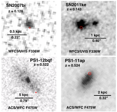
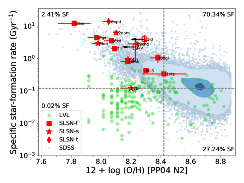
Figure 5: Left, from Lunnan et al. (2015): HST images of four SLSN host galaxies, showing their compact and often irregular morphologies. Right, from Chen et al. (2017a): Star-formation rate per unit mass versus metallicity (oxygen to hydrogen ratio). Compared to a magnitude-limited sample of galaxies from the Sloan Digitial sky survey, SLSNe occupy galaxies with low metallicity and high specific star-formation rate. In a volume limited sample, only $\approx 2\%$ of star-formation occurs in galaxies with metallicities less than $0.5\times$ the solar value, highlighting the importance of this parameter in producing SLSNe.

In contrast to most supernovae, SLSNe occur almost exclusively in low-mass dwarf galaxies. Example SLSN host galaxies, imaged with HST by Lunnan et al. (2015), are shown in Figure 5. Since one might naturally have assumed that rare events would be more likely to occur in regions of high stellar mass, this surprising preference for dwarf galaxies must be a clue to their nature.

Two main physical conditions have been identified in SLSN hosts, and proposed to account for SLSN production: high specific (i.e. per unit mass) star-formation rate (sSFR), and low metallicities (Neill et al., 2011; Chen et al., 2013; Lunnan et al., 2014; Leloudas et al., 2015a; Chen et al., 2015; Angus et al., 2016). From current samples of SLSN hosts, it appears that the SLSN rate is strongly suppressed at metallicities $\gtrsim 0.5$ Z_⊙, where Z_⊙ is the solar ratio of oxygen to hydrogen (Perley et al., 2016; Chen et al., 2017a; Schulze et al., 2018). As shown in Figure 5, only 2% of star-formation in a volume-limited sample occurs at such low metallicity, helping to account for the rarity of SLSNe. However, SLSNe at high metallicity are not impossible, with two (out of $\sim 100$ known) having occurred in massive, metal-rich galaxies (Perley et al., 2016; Bose et al., 2018). The preference for low metallicities and high sSFR is reminiscent of long GRB host galaxies (Lunnan et al., 2014), although long GRBs appear to have a higher metallicity threshold, $\sim\,$Z_⊙, before they are suppressed (Graham & Fruchter, 2013; Krühler et al., 2015; Schulze et al., 2018).

The high sSFRs may be necessary to form very massive stars – either probabilistically, by sampling the initial mass function more rapidly, or by modifying it to produce a larger fraction of very massive stars. Or, it may simply be an artefact of dwarf galaxies tending to form their stars in bursts (Perley et al., 2016). Many SLSN hosts have been identified as ‘extreme emission line’ galaxies, suggesting a strong ionising radiation field could impact the progenitor evolution (Leloudas et al., 2015a; Thone et al., 2015). Interactions between SLSN hosts and nearby galaxies may also be important in triggering or modifying star formation (Chen et al., 2017b), with up to 50% of SLSN hosts having a companion galaxy within 5 kpc (Ørum et al., 2020).

4.4 Non-thermal emission

SLSNe emit the bulk of their luminosity thermally, in the UV and optical bands. Searches for non-thermal X-ray and radio emission have provided additional clues to their nature, despite yielding mostly non-detections. Margutti et al. (2018) surveyed 26 SLSNe in X-rays, on timescales from days to years after explosion. They detected the SLSN PTF12dam using the Chandra X-ray Observatory, at an X-ray luminosity $L_{\rm X}\approx 2\times 10^{40}$ erg s^-1 around the time of its optical peak, and derived upper limits $L_{\rm X}\lesssim 10^{41}$ erg s^-1 for virtually all other events. Thus typical SLSNe are at least 100 times fainter in X-rays than in the optical. The only (spectroscopically-normal) SLSN to violate this rule is SCP06F6, with $L_{\rm X}\sim 10^{45}$ erg s^-1 (Levan et al., 2013). It was suggested by Metzger et al. (2014) that the X-rays in SCP06F6 may have occurred as a result of the engine-powered ionization breakout discussed above.

The story is similar in the radio. Coppejans et al. (2018) compiled all SLSN radio observations at that time (nine events), with no detections. The deepest limits, $\nu L_{\nu}\lesssim{\rm few}\times 10^{36}$ erg s^-1, are for the very nearby SN2017egm (Bose et al., 2018). Eftekhari et al. (2021) observed 36 SLSNe with the Very Large Array (VLA) and Atacama Millimeter/Submillimeter Array (ALMA). Their VLA detection of PTF10hgi at 7.5 years after explosion, with $\nu L_{\nu}\approx 6\times 10^{37}$ erg s^-1 at 6 GHz, is the only radio detection in their sample (Eftekhari et al., 2019), and this event remains the only SLSN detected in the radio. The observed emission was consistent with either a pulsar wind nebula energised by a magnetar, or an off-axis jet spreading into our line of sight (in either case, a sign of a central engine). The magnetar hypothesis is supported by additional studies from Law et al. (2019); Mondal et al. (2020). SLSN ejecta is expected to become optically thin to magnetar-powered radio emission only after years to decades, so this picture can be confirmed by continuing to observe the known SLSNe as they age (Margalit et al., 2018b; Omand et al., 2018). Intriguingly, the radio emission from PTF10hgi also resembles the persistent source associated with the first repeating Fast Radio Burst (FRB), FRB121102 (Chatterjee et al., 2017), which resides in a dwarf galaxy similar to SLSN hosts. This has prompted speculation that at least some FRBs originate from the remnants of SLSNe (Metzger et al., 2017; Nicholl et al., 2017b), although subsequent FRB localisations have not shown the same host galaxy preferences. No FRB flares have yet been detected during radio observations of SLSNe.

The numerous non-detections of SLSNe in the X-ray and radio have been used to place tight limits on the density of CSM. In normal CCSNe, the non-thermal emission is synchrotron radiation produced as the blast wave passes through the external medium; it is sensitive to the particle density and the energy of the shock (Chevalier & Fransson, 1994; Weiler et al., 2002). The non-thermal emission from a normal SN Ic would be too faint to detect at the distances of most SLSNe, however radio limits for SN2017egm showed that it would be at the faint end even for SNe Ic, which have pre-explosion mass-loss rates $\lesssim 10^{-5}$ M_⊙ yr^-1 (e.g. Berger et al., 2002), assuming Wolf-Rayet star wind velocities $\sim 1000$ km s^-1. Similarly, radio limits for SN2015bn from 1-3 years post-explosion ruled out mass-loss rates in the range $\sim 10^{-5}-10^{-3}$ M_⊙ yr^-1, i.e. excluding a wind significantly more dense than a normal supernova progenitor (Nicholl et al., 2018). X-ray limits have been used to similarly constrain the wind mass-loss rate $\lesssim 10^{-5}-10^{-2}$ M_⊙ yr^-1 (Margutti et al., 2018), or the total shocked CSM mass $\lesssim 0.1$ M_⊙ (Inserra et al., 2017).

In a GRB afterglow, non-thermal emission is produced when jets, driven by a magnetar (Thompson et al., 2004) or accreting black hole engine (MacFadyen & Woosley, 1999), shock the surrounding medium. This produces X-ray and radio emission orders of magnitude brighter than in ordinary supernovae, though the luminosity and the timescale for the afterglow to become visible depend on the orientation of the jet relative to the observer (Mészáros & Rees, 1997). Detecting jets from SLSNe would be one way to confirm that a central engine operates in these events too, especially in light of their similar hosts to long GRBs, and mutual spectroscopic connection to SNe Ic. Eftekhari et al. (2021) rule out even off-axis jets for 10 SLSNe, and greatly restrict the viable parameter space in jet energy and ambient density for several others, suggesting most SLSNe do not launch successful jets. However, this may be unsurprising even in the magnetar-powered scenario: powering a GRB jet requires that the engine rapidly supply its energy on a timescale of seconds, whereas to continuously heat the ejecta and power a SLSN requires that the engine release its energy on a timescale comparable to $t_{\rm peak}$. The discovery of SN2011kl, a supernova approaching SLSN luminosities, in conjunction with a very rare ‘ultra-long’ GRB lasting for $\sim 10,000$ s (Greiner et al., 2015) may represent a transitional event where an engine with an intermediate lifetime manages to power both a jet and a luminous supernova (Metzger et al., 2015; Gompertz & Fruchter, 2017; Kann et al., 2019).

4.5 Polarimetry

The polarisation of light emitted from a supernova is a probe of its geometry (e.g. see review by Wang & Wheeler, 2008): an asymmetric distribution of material produces a net polarisation. Asymmetries could arise due to e.g. bipolar outflows (possibly from failed jets), or a non-uniform distribution of CSM. A handful of SLSNe have now been observed using both imaging- and spectro-polarimetry. In the cases of LSQ14mo, SN2018hti, PS17bek and OGLE16dmu, no intrinsic polarisation could be identified above the interstellar polarisation induced by intervening dust (Leloudas et al., 2015b; Lee, 2019; Cikota et al., 2018). However, high quality polarimetric observations of SN2015bn (Inserra et al., 2016; Leloudas et al., 2017) and SN2017egm (Bose et al., 2018; Saito et al., 2020) have shown significant polarisation. In both cases, as the photosphere receded to deeper layers of the ejecta, the polarisation increased, indicating that the inner ejecta was more aspherical than the outer ejecta. In the case of SN2015bn, this transition was quite sudden and coincided with light curve undulations and cooling of the spectrum (Leloudas et al., 2017). The increasing asymmetry has been interpreted as a possible sign of central energy injection along a dominant axis (Inserra et al., 2016; Saito et al., 2020).

4.6 Nebular phase observations

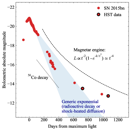
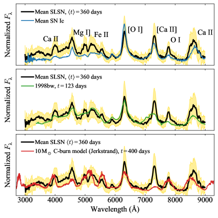
Figure 6: Long-term observations of SLSNe. Left: the light curve slopes predicted by different models diverge at $\sim$ hundreds of days after explosion. Two SLSNe with HST imaging in this phase show a flattening consistent with magnetar engines (Nicholl et al., 2018; Blanchard et al., 2021). Right: Average spectrum at one year after explosion, when the ejecta have become transparent, compared to normal SNe Ic (top), the GRB-supernova 1998bw (middle) and a model from Jerkstrand et al. (2017) (bottom). The strongest emission lines are labelled; the square-bracket notation indicates ‘forbidden’ lines, i.e. unlikely transitions that can only occur in low-density gas. SLSNe and GRB-supernovae show strong iron lines below $\sim 5000$ Å, pointing to more massive progenitors than normal SNe Ic. The strong oxygen and calcium lines are consistent with clumpy ejecta and a central heating source (Jerkstrand et al., 2017; Nicholl et al., 2019).

As supernovae expand and cool, the photosphere continues to recede deeper into the ejecta. By a time

$$t_{\rm neb}\sim 1\,{\rm year}\ (M_{\rm ej}/10\,{\rm M}_{\odot})^{1/2}\ (v_{\rm ej}/10^{4}\,{\rm km}\,{\rm s}^{-1})^{-1},$$ (6)

the ejecta become fully transparent and the so-called ‘nebular phase’ begins. There is no longer an electron-scattering blackbody continuum or absorption lines. Instead, various (permitted and forbidden) emission lines appear as the electron density drops below critical values (see review by Jerkstrand, 2017). The first nebular spectrum of an SLSN was obtained for SN2007bi by Gal-Yam et al. (2009). By 2019, the nebular sample had grown to 12 events, with the majority from PTF (Quimby et al., 2018), enabling the first statistical studies (Nicholl et al., 2019). The mean nebular spectrum of SLSNe is shown in Figure 6. The observed emission lines are the same as in SNe Ic, however the strength of the iron lines from 4000-5000 Å is significantly enhanced in SLSNe, similar to nebular observations of broad-lined SNe Ic associated with long GRBs (Nicholl et al., 2016b; Jerkstrand et al., 2017). The O I $\lambda$7774 recombination line is stronger in SLSNe than in normal or broad-lined SNe Ic. Its luminosity combined with its narrow velocity width indicates ongoing ionisation in the inner regions of the ejecta, likely requiring continuous central energy injection (Milisavljevic et al., 2013; Nicholl et al., 2016b; Nicholl et al., 2019).

Model spectra of slowly-evolving SLSNe computed by Jerkstrand et al. (2017) showed that most of the lines can be reproduced by $\sim 10$ M_⊙of explosive carbon-burning products (which are mostly oxygen by mass). They also determined from calcium line ratios that SLSN ejecta must be significantly ‘clumped’, i.e. consisting of compact dense regions in an otherwise rarified volume. Evidence for clumping was further observed in a larger sample of events, and the electron density within the clumps ($n_{e}>10^{8}$ cm^-3) helps to account for the strength of the O I recombination line (Nicholl et al., 2019). Clumping can arise due to engine-driven pressure instabilities (Kasen & Bildsten, 2010; Chen et al., 2016), but may also occur due to fragmentation of a cold dense shell at an eject-CSM interface (though Jerkstrand et al. 2017 note that it could be difficult to encompass enough mass in this shell). An outstanding mystery in SLSNe is why some events show apparently nebular emission from [Ca II] much earlier, during the photospheric phase (Gal-Yam et al., 2009; Inserra et al., 2017) – this requires some part of the ejecta to become rarified much more rapidly than in conventional supernovae.

Following SLSNe deeper into the nebular phase provides another handle on the heating source. As shown in Figure 6, radioactivity, magnetar spin-down, and CSM interaction diverge in their predictions for the light curve slope, though distinguishing between them robustly requires observations years after explosion (Woosley, 2010; Inserra et al., 2013; Moriya et al., 2017). Such observations have now been obtained with the Hubble Space Telescope (HST) for SN2015bn (Nicholl et al., 2018) and SN2016inl (Blanchard et al., 2021) at phases of $\approx 500-1000$ days. The data appear to most closely track the magnetar spin-down scenario, but prefer steeper power-law indices $L\propto t^{-\alpha}$ with $\alpha=3-4$ rather than the fiducial $\alpha=2$ (equation 4). This can be explained if a fraction of the engine power ‘leaks’ out of the ejecta without heating it; as the ejecta become less dense, a larger fraction escapes (Wang et al., 2015; Chen et al., 2015; Nicholl et al., 2018). Deep upper limits in X-rays (Bhirombhakdi et al., 2018) and radio (Nicholl et al., 2018) at the same phase as the optical detections of SN2015bn showed that $\lesssim 1\%$ of the available engine energy could be escaping in these wavelengths. Given the hard spectrum expected from a magnetar, GeV-TeV gamma-rays are the most likely waveband for leakage; upper limits from the Fermi satellite have not yet been deep enough to rule this out (Renault-Tinacci et al., 2018). However, recent simulations by Vurm & Metzger (2021) showed that gamma-ray escape on timescales of $\sim 1$ year require low magnetization of the expanding nebula, potentially posing difficulties for the ‘leaky magnetar’ picture.

5 Diversity and progenitors

SLSNe appear to originate from stars more massive than typical CCSN progenitors: this is evidenced by their longer durations (and implied ejecta masses), nebular spectra with strong [O I] and Fe II emission, and the intensely star-forming environments in which they occur. Based on light curve fits assuming a magnetar model, Blanchard et al. (2020) estimated pre-explosion progenitor masses (corresponding to the carbon-oxygen core of the stripped star) in the range 3.6–40 M_⊙. A steep drop-off at the top of this range may indicate an upper limit where the progenitor encounters the pulsational pair-instability. In contrast, the progenitors of normal CCSNe mostly fall below $\lesssim 20$ M_⊙ (e.g. Smartt, 2009). To eject the highest masses inferred in SLSNe, especially at the observed high velocities, likely requires an explosion energy $\sim 10^{52}$ erg, an order of magnitude greater than the canonical energy scale for normal supernovae (Blanchard et al., 2020; Mazzali et al., 2016).

The spectroscopic (especially in the nebular phase) and host galaxy connections between SLSNe and long GRBs could indicate that SLSNe have similar progenitors and/or explosion mechanisms to the engine-powered GRBs. Assuming a magnetar engine, Figure 7 shows how slower evolving SLSNe can be explained by higher ejecta masses and weaker magnetic fields. Nicholl et al. (2017c) noted that at least some of the diversity in SLSN spectra at maximum light may be a result of longer rise times in more massive events, leading to a larger photosphere and cooler temperature for a similar luminosity and velocity. Although the magnetar model has been criticised as overly flexible, in fact it has the minimum number of extra parameters to decouple the peak luminosity from the timescale, and produce more diverse light curves than radioactive models ($P$ and $B$ rather than just $M_{\rm Ni}$), and fewer parameters than CSM interaction models. Given the observed diversity in SLSNe, an extra degree of freedom is not arbitrary, but rather a necessary and sufficient physical condition.

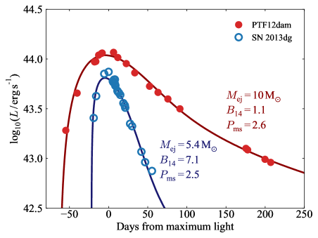
Figure 7: Left: Diverse SLSN light curves fitted with magnetar models. More massive ejecta and lower magnetic fields lead to slower evolution, and the longer rise time results in a larger maximum light radius and a cooler spectrum for the same luminosity. Right, from Blanchard et al. (2020): Ejecta mass versus magnetar spin period from model fits to 62 SLSNe. The observed correlation could be explained by mass-stripping: progenitors that lose more mass before explosion also lose more angular momentum. The results are consistent with simulations by Aguilera-Dena et al. (2018).

Nicholl et al. (2017c) suggested that the relative rate of SLSNe compared to normal CCSNe is consistent with the small fractional volume of mass-spin-magnetic field space that produces over-luminous events. For $B\gtrsim 10^{15}$ G, the energy would be injected in seconds rather than days, driving a GRB jet rather than a SLSN (Metzger et al., 2015). For $B\lesssim 10^{13}$ G, the magnetar spins down too slowly to boost the energy or peak luminosity of the supernova, producing only a normal SN Ic. In this case evidence of the magnetar could still appear in the late-time light curve, as was possibly seen in the SN Ic iPTF15dtg (Taddia et al., 2019). A continuum of magnetic field strengths (or spin periods) predicts a continuum of luminosities between the various classes of stripped supernovae, and in fact this is now observed in unbiased supernova samples (De Cia et al., 2018).

If central engines are the key ingredient for making SLSNe, their progenitors must be rapidly rotating. Simulations show that if the core is spinning fast enough at collapse to make a millisecond neutron star, a dynamo mechanism can naturally amplify the magnetic field to the range required for SLSNe (Duncan & Thompson, 1992; Mösta et al., 2015). The low-metallicity environments where most events are located help to reduce angular momentum loss from metallicity-dependent, line-driven stellar winds (e.g. Vink & Sander, 2021). However, since SLSNe (and GRB-supernovae) lack hydrogen, they must have lost their envelopes somehow. Woosley (2017) found that rapidly-spinning single-star models with initial masses in the range 60–100 M_⊙ can retain high core angular momentum even after losing their envelopes via pair-instability pulsations. Rotation also leads to more massive cores by mixing in fresh material from the envelope. Interaction with a close binary companion could offer an alternative pathway to remove the envelope while maintaining (or even spinning up) the rotation of the progenitor (e.g. Yoon et al., 2010; de Mink et al., 2013). Stevance & Eldridge (2021) identified plausible binary progenitor models for the SLSN 2017gci, but could find no viable single star scenarios within their library of population synthesis models.

The connections between binary interaction, rotation, core mass and envelope loss may underpin much of the diversity in SLSNe. Chen et al. (2017a) identified a possible correlation between magnetar spin periods (from model fits to SLSN data) and host metallicity, which could be explained by more mass-stripping in metal-rich environments, though this was not recovered in other studies (Nicholl et al., 2017c; De Cia et al., 2018). Blanchard et al. (2020) found an anti-correlation between ejected mass and spin period, consistent with more heavily stripped stars having lost more angular momentum (Figure 7). This correlation has also been found by Aguilera-Dena et al. (2018, 2020) in their simulations of rapidly rotating massive stars. These models also predict $\sim 0.5$ M_⊙ of CSM close to the progenitor, due to rotational and neutrino-driven mass-loss during late burning stages. This mass of CSM, and the timing of ejection, is compatible with the undulations in some SLSN light curves. A consistent picture may be emerging in which differing degrees of CSM interaction add another layer of complexity to SLSN observables, on top of the underlying variation from different ejecta and engine parameters.

6 Looking ahead

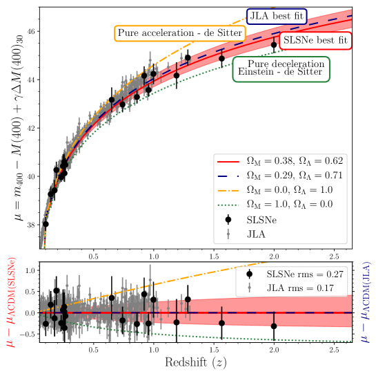
Figure 8: From Inserra et al. (2021): Hubble diagram (distance vs redshift) for SLSNe (black) and SNe Ia (grey). Supernova cosmology relies on determining the true peak luminosity of an event from a distance-independent parameter such as light curve width (a ‘standardisable candle’). Comparing the observed and intrinsic brightness gives the distance. The redshift, derived from the spectrum, measures how quickly the Universe is expanding at that distance. Because of their luminosity, SLSNe can be detected at much greater distances than SNe Ia. If they can be standardised, they enable measurements of the expansion history of the Universe at earlier times when differences between cosmological models are more pronounced.

We are now entering the statistical age of SLSNe. The new Vera Rubin Observatory, conducting the Legacy Survey of Space and Time (LSST), is predicted to find $\sim 10^{4}$ SLSNe per year (Villar et al., 2018). Machine learning techniques will be required to separate SLSNe from other transients in this enormous data stream (e.g. Gomez et al., 2020; Villar et al., 2020; Hosseinzadeh et al., 2020; Muthukrishna et al., 2019), and enable spectroscopic and multi-wavelength follow-up. With thousands of SLSNe, we will much more finely sample their diversity and energetics, and continue to pin down their progenitors. As the first wide-field survey with an 8 m telescope, LSST will be especially important in building up the sample at higher redshift. SLSNe are detectable at much greater distances than other transient types, with a handful of known events at redshifts $z\sim 2-4$ (Cooke et al., 2012; Pan et al., 2017; Smith et al., 2018; Moriya et al., 2019; Curtin et al., 2019). Increasing these numbers will enable us to probe conditions and star formation in the early Universe (Berger et al., 2012) and to extend supernova cosmology beyond the reach of SNe Ia (Inserra & Smartt, 2014; Inserra et al., 2021, Figure 8).

When it comes to SLSN physics, progress requires a better understanding of how the engine – if indeed one is present – releases its energy to the ejecta. This could be in the form of a particle wind, Poynting flux, or magnetic reconnection (e.g. Margalit et al., 2018a; Vurm & Metzger, 2021). Detecting or ruling out high-energy leakage at late times will provide important constraints. It is equally important to determine the fraction of SLSNe that interact with CSM, and to establish a more robust mapping between the CSM properties and their effect on SLSN observables, allowing us to trace out the final decades in the lives of these stars via the material expelled during this time. Observations within the first days after explosion, made more feasible by the deep imaging from LSST, will probe material even closer to the progenitor, reveal the nature of the light curve ‘bumps’, and – hopefully – produce even more surprises.

References

- Aguilera-Dena et al. (2018) Aguilera-Dena D. R., Langer N., Moriya T. J., Schootemeijer A., 2018, ApJ, 858, 115
- Aguilera-Dena et al. (2020) Aguilera-Dena D. R., Langer N., Antoniadis J., Müller B., 2020, ApJ, 901, 114
- Anderson et al. (2018) Anderson J. P., et al., 2018, A&A, 620, A67
- Angus et al. (2016) Angus C. R., Levan A. J., Perley D. A., Tanvir N. R., Lyman J. D., Stanway E. R., Fruchter A. S., 2016, MNRAS, 458, 84
- Angus et al. (2019) Angus C. R., et al., 2019, MNRAS, 487, 2215
- Arnett (1982) Arnett W. D., 1982, ApJ, 253, 785
- Barbary et al. (2009) Barbary K., et al., 2009, ApJ, 690, 1358
- Barkat et al. (1967) Barkat Z., Rakavy G., Sack N., 1967, Phys. Rev. Lett., 18, 379
- Bellm et al. (2019) Bellm E. C., et al., 2019, PASP, 131, 018002
- Benetti et al. (2014) Benetti S., et al., 2014, MNRAS, 441, 289
- Berger et al. (2002) Berger E., Kulkarni S. R., Chevalier R. A., 2002, ApJ, 577, L5
- Berger et al. (2003) Berger E., Kulkarni S. R., Frail D. A., Soderberg A. M., 2003, ApJ, 599, 408
- Berger et al. (2012) Berger E., et al., 2012, ApJ, 755, L29
- Bhirombhakdi et al. (2018) Bhirombhakdi K., Chornock R., Margutti R., Nicholl M., Metzger B. D., Berger E., Margalit B., Milisavljevic D., 2018, ApJ, 868, L32
- Blanchard et al. (2018) Blanchard P. K., et al., 2018, ApJ, 865, 9
- Blanchard et al. (2019) Blanchard P. K., Nicholl M., Berger E., Chornock R., Milisavljevic D., Margutti R., Gomez S., 2019, ApJ, 872, 90
- Blanchard et al. (2020) Blanchard P. K., Berger E., Nicholl M., Villar V. A., 2020, ApJ, 897, 114
- Blanchard et al. (2021) Blanchard P. K., Berger E., Nicholl M., Chornock R., Gomez S., Hosseinzadeh G., 2021, arXiv e-prints, p. arXiv:2105.03475
- Bose et al. (2018) Bose S., et al., 2018, ApJ, 853, 57
- Branch et al. (2000) Branch D., Jeffery D. J., Blaylock M., Hatano K., 2000, PASP, 112, 217
- Chatterjee et al. (2017) Chatterjee S., et al., 2017, Nature, 541, 58
- Chatzopoulos et al. (2011) Chatzopoulos E., et al., 2011, ApJ, 729, 143
- Chatzopoulos et al. (2012) Chatzopoulos E., Wheeler J. C., Vinko J., 2012, ApJ, 746, 121
- Chen (2021) Chen K.-J., 2021, International Journal of Modern Physics D, 30, 2130001
- Chen et al. (2013) Chen T.-W., et al., 2013, ApJ, 763, L28
- Chen et al. (2015) Chen T. W., et al., 2015, MNRAS, 452, 1567
- Chen et al. (2016) Chen K.-J., Woosley S. E., Sukhbold T., 2016, ApJ, 832, 73
- Chen et al. (2017a) Chen T.-W., Smartt S. J., Yates R. M., Nicholl M., Krühler T., Schady P., Dennefeld M., Inserra C., 2017a, MNRAS, 470, 3566
- Chen et al. (2017b) Chen T. W., et al., 2017b, A&A, 602, A9
- Chen et al. (2018) Chen T. W., et al., 2018, ApJ, 867, L31
- Chevalier & Fransson (1994) Chevalier R. A., Fransson C., 1994, ApJ, 420, 268
- Chevalier & Irwin (2011) Chevalier R. A., Irwin C. M., 2011, ApJ, 729, L6
- Childress et al. (2015) Childress M. J., et al., 2015, MNRAS, 454, 3816
- Chomiuk et al. (2011) Chomiuk L., et al., 2011, ApJ, 743, 114
- Cikota et al. (2018) Cikota A., et al., 2018, MNRAS, 479, 4984
- Cooke et al. (2012) Cooke J., et al., 2012, Nature, 491, 228
- Coppejans et al. (2018) Coppejans D. L., et al., 2018, ApJ, 856, 56
- Crowther (2007) Crowther P. A., 2007, ARA&A, 45, 177
- Curtin et al. (2019) Curtin C., et al., 2019, ApJS, 241, 17
- De Cia et al. (2018) De Cia A., et al., 2018, ApJ, 860, 100
- Dessart (2019) Dessart L., 2019, A&A, 621, A141
- Dessart et al. (2012) Dessart L., Hillier D. J., Waldman R., Livne E., Blondin S., 2012, MNRAS, 426, L76
- Dessart et al. (2013) Dessart L., Waldman R., Livne E., Hillier D. J., Blondin S., 2013, MNRAS, 428, 3227
- Dexter & Kasen (2013) Dexter J., Kasen D., 2013, ApJ, 772, 30
- Drake et al. (2009) Drake A. J., et al., 2009, ApJ, 696, 870
- Drake et al. (2010) Drake A. J., et al., 2010, ApJ, 718, L127
- Drout et al. (2011) Drout M. R., et al., 2011, ApJ, 741, 97
- Duncan & Thompson (1992) Duncan R. C., Thompson C., 1992, ApJ, 392, L9
- Eftekhari et al. (2019) Eftekhari T., et al., 2019, ApJ, 876, L10
- Eftekhari et al. (2021) Eftekhari T., et al., 2021, ApJ, 912, 21
- Fiore et al. (2021) Fiore A., et al., 2021, MNRAS, 502, 2120
- Frohmaier et al. (2021) Frohmaier C., et al., 2021, MNRAS, 500, 5142
- Gal-Yam (2012) Gal-Yam A., 2012, Science, 337, 927
- Gal-Yam (2019a) Gal-Yam A., 2019a, ARA&A, 57, 305
- Gal-Yam (2019b) Gal-Yam A., 2019b, ApJ, 882, 102
- Gal-Yam et al. (2009) Gal-Yam A., et al., 2009, Nature, 462, 624
- Gezari et al. (2009) Gezari S., et al., 2009, ApJ, 690, 1313
- Ginzburg & Balberg (2012) Ginzburg S., Balberg S., 2012, ApJ, 757, 178
- Gomez et al. (2020) Gomez S., Berger E., Blanchard P. K., Hosseinzadeh G., Nicholl M., Villar V. A., Yin Y., 2020, ApJ, 904, 74
- Gompertz & Fruchter (2017) Gompertz B., Fruchter A., 2017, ApJ, 839, 49
- Graham & Fruchter (2013) Graham J. F., Fruchter A. S., 2013, ApJ, 774, 119
- Greiner et al. (2015) Greiner J., et al., 2015, Nature, 523, 189
- Heger & Woosley (2002) Heger A., Woosley S. E., 2002, ApJ, 567, 532
- Hodgkin et al. (2021) Hodgkin S. T., et al., 2021, arXiv e-prints, p. arXiv:2106.01394
- Hosseinzadeh et al. (2020) Hosseinzadeh G., et al., 2020, ApJ, 905, 93
- Howell (2017) Howell D. A., 2017, Superluminous Supernovae. p. 431, doi:10.1007/978-3-319-21846-5_41
- Howell et al. (2013) Howell D. A., et al., 2013, ApJ, 779, 98
- Inserra (2019) Inserra C., 2019, Nature Astronomy, 3, 697
- Inserra & Smartt (2014) Inserra C., Smartt S. J., 2014, ApJ, 796, 87
- Inserra et al. (2013) Inserra C., et al., 2013, ApJ, 770, 128
- Inserra et al. (2016) Inserra C., Bulla M., Sim S. A., Smartt S. J., 2016, ApJ, 831, 79
- Inserra et al. (2017) Inserra C., et al., 2017, MNRAS, 468, 4642
- Inserra et al. (2018a) Inserra C., et al., 2018a, MNRAS, 475, 1046
- Inserra et al. (2018b) Inserra C., Prajs S., Gutierrez C. P., Angus C., Smith M., Sullivan M., 2018b, ApJ, 854, 175
- Inserra et al. (2021) Inserra C., et al., 2021, MNRAS,
- Jerkstrand (2017) Jerkstrand A., 2017, Spectra of Supernovae in the Nebular Phase. p. 795, doi:10.1007/978-3-319-21846-5_29
- Jerkstrand et al. (2017) Jerkstrand A., et al., 2017, ApJ, 835, 13
- Kaiser et al. (2010) Kaiser N., et al., 2010, in Stepp L. M., Gilmozzi R., Hall H. J., eds, Society of Photo-Optical Instrumentation Engineers (SPIE) Conference Series Vol. 7733, Ground-based and Airborne Telescopes III. p. 77330E, doi:10.1117/12.859188
- Kann et al. (2019) Kann D. A., et al., 2019, A&A, 624, A143
- Kasen & Bildsten (2010) Kasen D., Bildsten L., 2010, ApJ, 717, 245
- Kasen et al. (2011) Kasen D., Woosley S. E., Heger A., 2011, ApJ, 734, 102
- Kasen et al. (2016) Kasen D., Metzger B. D., Bildsten L., 2016, ApJ, 821, 36
- Kozyreva & Blinnikov (2015) Kozyreva A., Blinnikov S., 2015, MNRAS, 454, 4357
- Krühler et al. (2015) Krühler T., et al., 2015, A&A, 581, A125
- Law et al. (2019) Law C. J., et al., 2019, ApJ, 886, 24
- Lee (2019) Lee C.-H., 2019, ApJ, 875, 121
- Leloudas et al. (2012) Leloudas G., et al., 2012, A&A, 541, A129
- Leloudas et al. (2015a) Leloudas G., et al., 2015a, MNRAS, 449, 917
- Leloudas et al. (2015b) Leloudas G., et al., 2015b, ApJ, 815, L10
- Leloudas et al. (2017) Leloudas G., et al., 2017, ApJ, 837, L14
- Levan et al. (2013) Levan A. J., Read A. M., Metzger B. D., Wheatley P. J., Tanvir N. R., 2013, ApJ, 771, 136
- Liu et al. (2017) Liu Y.-Q., Modjaz M., Bianco F. B., 2017, ApJ, 845, 85
- Lunnan et al. (2014) Lunnan R., et al., 2014, ApJ, 787, 138
- Lunnan et al. (2015) Lunnan R., et al., 2015, ApJ, 804, 90
- Lunnan et al. (2016) Lunnan R., et al., 2016, ApJ, 831, 144
- Lunnan et al. (2018a) Lunnan R., et al., 2018a, Nature Astronomy, 2, 887
- Lunnan et al. (2018b) Lunnan R., et al., 2018b, ApJ, 852, 81
- Lunnan et al. (2020) Lunnan R., et al., 2020, ApJ, 901, 61
- MacFadyen & Woosley (1999) MacFadyen A. I., Woosley S. E., 1999, ApJ, 524, 262
- Margalit et al. (2018a) Margalit B., Metzger B. D., Thompson T. A., Nicholl M., Sukhbold T., 2018a, MNRAS, 475, 2659
- Margalit et al. (2018b) Margalit B., Metzger B. D., Berger E., Nicholl M., Eftekhari T., Margutti R., 2018b, MNRAS, 481, 2407
- Margutti et al. (2018) Margutti R., et al., 2018, ApJ, 864, 45
- Mazzali et al. (2016) Mazzali P. A., Sullivan M., Pian E., Greiner J., Kann D. A., 2016, MNRAS, 458, 3455
- Mészáros & Rees (1997) Mészáros P., Rees M. J., 1997, ApJ, 476, 232
- Metzger et al. (2014) Metzger B. D., Vurm I., Hascoët R., Beloborodov A. M., 2014, MNRAS, 437, 703
- Metzger et al. (2015) Metzger B. D., Margalit B., Kasen D., Quataert E., 2015, MNRAS, 454, 3311
- Metzger et al. (2017) Metzger B. D., Berger E., Margalit B., 2017, ApJ, 841, 14
- Milisavljevic et al. (2013) Milisavljevic D., et al., 2013, ApJ, 770, L38
- Miller et al. (2009) Miller A. A., et al., 2009, ApJ, 690, 1303
- Mondal et al. (2020) Mondal S., Bera A., Chandra P., Das B., 2020, MNRAS, 498, 3863
- Moriya & Maeda (2012) Moriya T. J., Maeda K., 2012, ApJ, 756, L22
- Moriya et al. (2017) Moriya T. J., Chen T.-W., Langer N., 2017, ApJ, 835, 177
- Moriya et al. (2018a) Moriya T. J., Sorokina E. I., Chevalier R. A., 2018a, Space Sci. Rev., 214, 59
- Moriya et al. (2018b) Moriya T. J., Nicholl M., Guillochon J., 2018b, ApJ, 867, 113
- Moriya et al. (2019) Moriya T. J., et al., 2019, ApJS, 241, 16
- Mösta et al. (2015) Mösta P., Ott C. D., Radice D., Roberts L. F., Schnetter E., Haas R., 2015, Nature, 528, 376
- Muthukrishna et al. (2019) Muthukrishna D., Narayan G., Mandel K. S., Biswas R., Hložek R., 2019, PASP, 131, 118002
- Nadyozhin (1994) Nadyozhin D. K., 1994, ApJS, 92, 527
- Neill et al. (2011) Neill J. D., et al., 2011, ApJ, 727, 15
- Nicholl & Smartt (2016) Nicholl M., Smartt S. J., 2016, MNRAS, 457, L79
- Nicholl et al. (2013) Nicholl M., et al., 2013, Nature, 502, 346
- Nicholl et al. (2015a) Nicholl M., et al., 2015a, MNRAS, 452, 3869
- Nicholl et al. (2015b) Nicholl M., et al., 2015b, ApJ, 807, L18
- Nicholl et al. (2016a) Nicholl M., et al., 2016a, ApJ, 826, 39
- Nicholl et al. (2016b) Nicholl M., et al., 2016b, ApJ, 828, L18
- Nicholl et al. (2017a) Nicholl M., Berger E., Margutti R., Blanchard P. K., Milisavljevic D., Challis P., Metzger B. D., Chornock R., 2017a, ApJ, 835, L8
- Nicholl et al. (2017b) Nicholl M., Williams P. K. G., Berger E., Villar V. A., Alexander K. D., Eftekhari T., Metzger B. D., 2017b, ApJ, 843, 84
- Nicholl et al. (2017c) Nicholl M., Guillochon J., Berger E., 2017c, ApJ, 850, 55
- Nicholl et al. (2018) Nicholl M., et al., 2018, ApJ, 866, L24
- Nicholl et al. (2019) Nicholl M., Berger E., Blanchard P. K., Gomez S., Chornock R., 2019, ApJ, 871, 102
- Nicholl et al. (2020) Nicholl M., et al., 2020, Nature Astronomy, 4, 893
- Ofek et al. (2007) Ofek E. O., et al., 2007, ApJ, 659, L13
- Omand et al. (2018) Omand C. M. B., Kashiyama K., Murase K., 2018, MNRAS, 474, 573
- Ørum et al. (2020) Ørum S. V., Ivens D. L., Strandberg P., Leloudas G., Man A. W. S., Schulze S., 2020, A&A, 643, A47
- Ostriker & Gunn (1971) Ostriker J. P., Gunn J. E., 1971, ApJ, 164, L95
- Pan et al. (2017) Pan Y. C., et al., 2017, MNRAS, 470, 4241
- Pastorello et al. (2010) Pastorello A., et al., 2010, ApJ, 724, L16
- Perley et al. (2016) Perley D. A., et al., 2016, ApJ, 830, 13
- Piro (2015) Piro A. L., 2015, ApJ, 808, L51
- Prentice et al. (2019) Prentice S. J., et al., 2019, MNRAS, 485, 1559
- Quimby et al. (2007) Quimby R. M., Aldering G., Wheeler J. C., Höflich P., Akerlof C. W., Rykoff E. S., 2007, ApJ, 668, L99
- Quimby et al. (2011) Quimby R. M., et al., 2011, Nature, 474, 487
- Quimby et al. (2013) Quimby R. M., Yuan F., Akerlof C., Wheeler J. C., 2013, MNRAS, 431, 912
- Quimby et al. (2018) Quimby R. M., et al., 2018, ApJ, 855, 2
- Rau et al. (2009) Rau A., et al., 2009, PASP, 121, 1334
- Renault-Tinacci et al. (2018) Renault-Tinacci N., Kotera K., Neronov A., Ando S., 2018, A&A, 611, A45
- Rest et al. (2011) Rest A., et al., 2011, ApJ, 729, 88
- Saito et al. (2020) Saito S., et al., 2020, ApJ, 894, 154
- Schlegel (1990) Schlegel E. M., 1990, MNRAS, 244, 269
- Schulze et al. (2018) Schulze S., et al., 2018, MNRAS, 473, 1258
- Shappee et al. (2014) Shappee B. J., et al., 2014, ApJ, 788, 48
- Smartt (2009) Smartt S. J., 2009, ARA&A, 47, 63
- Smith & McCray (2007) Smith N., McCray R., 2007, ApJ, 671, L17
- Smith et al. (2007) Smith N., et al., 2007, ApJ, 666, 1116
- Smith et al. (2016) Smith M., et al., 2016, ApJ, 818, L8
- Smith et al. (2018) Smith M., et al., 2018, ApJ, 854, 37
- Stevance & Eldridge (2021) Stevance H. F., Eldridge J. J., 2021, MNRAS,
- Suzuki & Maeda (2019) Suzuki A., Maeda K., 2019, ApJ, 880, 150
- Taddia et al. (2019) Taddia F., Sollerman J., Fremling C., Karamehmetoglu E., Barbarino C., Lunnan R., West S., Gal-Yam A., 2019, A&A, 621, A64
- Thompson & Duncan (1996) Thompson C., Duncan R. C., 1996, ApJ, 473, 322
- Thompson et al. (2004) Thompson T. A., Chang P., Quataert E., 2004, ApJ, 611, 380
- Thone et al. (2015) Thone C. C., de Ugarte Postigo A., Garcia-Benito R., Leloudas G., Schulze S., Amorin R., 2015, MNRAS, 451, L65
- Tonry et al. (2018) Tonry J. L., et al., 2018, PASP, 130, 064505
- Valenti et al. (2008) Valenti S., et al., 2008, ApJ, 673, L155
- Villar et al. (2018) Villar V. A., Nicholl M., Berger E., 2018, ApJ, 869, 166
- Villar et al. (2020) Villar V. A., et al., 2020, ApJ, 905, 94
- Vink & Sander (2021) Vink J. S., Sander A. A. C., 2021, MNRAS,
- Vreeswijk et al. (2014) Vreeswijk P. M., et al., 2014, ApJ, 797, 24
- Vreeswijk et al. (2017) Vreeswijk P. M., et al., 2017, ApJ, 835, 58
- Vurm & Metzger (2021) Vurm I., Metzger B. D., 2021, arXiv e-prints, p. arXiv:2101.05299
- Wang & Wheeler (2008) Wang L., Wheeler J. C., 2008, ARA&A, 46, 433
- Wang et al. (2015) Wang S. Q., Wang L. J., Dai Z. G., Wu X. F., 2015, ApJ, 799, 107
- Weiler et al. (2002) Weiler K. W., Panagia N., Montes M. J., Sramek R. A., 2002, ARA&A, 40, 387
- Woosley (2010) Woosley S. E., 2010, ApJ, 719, L204
- Woosley (2017) Woosley S. E., 2017, ApJ, 836, 244
- Woosley et al. (2007) Woosley S. E., Blinnikov S., Heger A., 2007, Nature, 450, 390
- Yan et al. (2015) Yan L., et al., 2015, ApJ, 814, 108
- Yan et al. (2017a) Yan L., et al., 2017a, ApJ, 840, 57
- Yan et al. (2017b) Yan L., et al., 2017b, ApJ, 848, 6
- Yan et al. (2018) Yan L., Perley D. A., De Cia A., Quimby R., Lunnan R., Rubin K. H. R., Brown P. J., 2018, ApJ, 858, 91
- Yan et al. (2020) Yan L., et al., 2020, ApJ, 902, L8
- Yoon et al. (2010) Yoon S. C., Woosley S. E., Langer N., 2010, ApJ, 725, 940
- Young et al. (2010) Young D. R., et al., 2010, A&A, 512, A70
- de Mink et al. (2013) de Mink S. E., Langer N., Izzard R. G., Sana H., de Koter A., 2013, ApJ, 764, 166