Segmentation of Brain MRI using an Altruistic Harris Hawks’ Optimization algorithm

Abstract

Segmentation is an essential requirement in medicine when digital images are used in illness diagnosis, especially, in posterior tasks as analysis and disease identification. An efficient segmentation of brain Magnetic Resonance Images (MRIs) is of prime concern to radiologists due to their poor illumination and other conditions related to de acquisition of the images. Thresholding is a popular method for segmentation that uses the histogram of an image to label different homogeneous groups of pixels into different classes. However, the computational cost increases exponentially according to the number of thresholds. In this paper, we perform the multi-level thresholding using an evolutionary metaheuristic. It is an improved version of the Harris Hawks Optimization (HHO) algorithm that combines the chaotic initialization and the concept of altruism. Further, for fitness assignment, we use a hybrid objective function where along with the cross-entropy minimization, we apply a new entropy function, and leverage weights to the two objective functions to form a new hybrid approach. The HHO was originally designed to solve numerical optimization problems. Earlier, the statistical results and comparisons have demonstrated that the HHO provides very promising results compared with well-established metaheuristic techniques. In this article, the altruism has been incorporated into the HHO algorithm to enhance its exploitation capabilities. We evaluate the proposed method over 10 benchmark images from the WBA database of the Harvard Medical School and 8 benchmark images from the Brainweb dataset using some standard evaluation metrics. On the Harvard WBA dataset, a Peak Signal to Noise Ratio (PSNR) of 26.61 and a Structural Similarity Index (SSIM) of 0.92 are achieved using 5 thresholds. For the same scenario, using the Brainweb dataset, a PSNR of 24.77 and SSIM of 0.86 are obtained. The obtained results justify the superiority of the proposed approach compared to existing state-of-the-art methods and baseline methods. The relevant codes for the proposed approach are available at: https://github.com/Rohit-Kundu/Segmentation-HHO_Altruism.

Segmentation of Brain MRI using an Altruistic Harris Hawks’ Optimization algorithm

Rajarshi Bandopadhyay

Department of Computer Science and Engineering, Jadavpur University

188, Raja S.C. Mullick Road, Kolkata-700032, West Bengal, INDIA

Email: rajarshibanerjee03@gmail.com

Rohit Kundu

Department of Electrical Engineering, Jadavpur University

188, Raja S.C. Mullick Road, Kolkata-700032, West Bengal, INDIA

Email: rohitkunduju@gmail.com

Diego Oliva*

Depto. Universidad de Guadalajara, CUCEI,

Av. Revolucion 1500, Guadalajara, Jal, MEXICO

Email: diego.oliva@cucei.udg.mx

and

School of Computer Science & Robotics,

Tomsk Polytechnic University, Tomsk, RUSSIA

Ram Sarkar

Department of Computer Science and Engineering, Jadavpur University

188, Raja S.C. Mullick Road, Kolkata-700032, West Bengal, INDIA

Email: ramjucse@gmail.com

*Corresponding author: Diego Oliva

*Corresponding author email: diego.oliva@cucei.udg.mx

1 Introduction

Recent advances in biomedical technologies allow the acquisition of medical images in different modalities, like Computer Tomography, Ultrasound and Magnetic Resonance Imaging (MRI). Brain MRI provides a high-resolution spatial image of the brain through a non-invasive test detailing its anatomical features. However, analyzing brain MRIs is an esoteric and time-consuming task that requires expert clinicians to manually extract important information. Moreover, such a method is prone to subjective variability which might delay or provide a wrong diagnosis of an obscure disease. Computer-Aided Diagnosis (CAD) tools are alternative solutions that can significantly reduce the time for such insidious disease identification.

Image segmentation is one of the most important preprocessing steps for medical image diagnosis [41, 19] which separates the object of interest from the whole image required for analyzing behavioural and morphological changes of the object to detect the disease. Image segmentation, in essence, classifies each pixel in an image into homogeneous groups, each of them shares some common characteristic such as intensity or texture. Brain MRI segmentation has influential clinical implications for early disease detection and prognosis. Accurate MRI segmentation leads to the visualization of different brain structures to delineate lesions, analyze brain development, plan surgeries and identify diseases such as dementia, schizophrenia, multiple sclerosis, and Alzheimer etc.

Thresholding is a simple, but efficient image segmentation procedure where the histogram of a grayscale image is used to distribute its pixels into different classes. For this, a distinct threshold ($th$) is set for establishing intensity values. The thresholding process can be distinguished into two categories, namely, binary thresholding, which uses a single $th$ value and multi-level thresholding, which uses multiple $th$ values. Binary (bi-level) thresholding is used for object recognition tasks, where the objects need to be separated from their background, whereas multi-level thresholding divides parts of an image into several classes. Thresholding methods can also be categorized into parametric and non-parametric approaches. Parametric approaches aim to estimate the parameters from a probability density function to separate the classes, while non-parametric techniques use intrinsic features of the image such as entropy and variance, which are optimized to find the ideal threshold values.

Unsupervised segmentation of brain MRIs is a popular area of research since in the biomedical domain, acquiring ground truth information for the images is difficult since it requires the expertise of trained medical professionals and preparation of ground truth is very tiresome. Baur et al. [7] used spatial auto-encoders with skip-connections for the unsupervised anomaly detection from brain MRI images. Singh et al. [52] proposed the “local Zernike moment and unbiased non-local means-based bias-corrected fuzzy C-means" method for unsupervised segmentation of brain MRIs which could deal with both noisy images and images containing intensity non-homogeneity artefacts. Bercea et al. [9] proposed a federated-learning based model, named “FedDis" for disentangling the parameter space into appearance and shape and share the shape parameter with the different parties which collaboratively train a machine learning model.

Several thresholding methods have also been proposed in the related literature like [1, 11, 24, 38]. Otsu’s thresholding method [39] is popularly used for histogram thresholding which uses the between-class variance for computing the optimal threshold value. Kapur’s entropy [22] thresholding method maximizes the entropy of the object and the background pixels to compute the optimal threshold. The minimum error thresholding method proposed by Cho et al. [12], assumes that the object and background pixels are normally distributed, thus defining and optimizing an objective function related to the Bayes risk. However, in such classical methods for threshold determination, the computational cost increases exponentially with the increase in thresholding levels [36]. Thus these classical methods are suitable only for a small number of thresholding levels like binary thresholding or up to two thresholds.

As an alternative to the classical methods, evolutionary meta-heuristics and swarm intelligence based algorithms have been widely used to address the multi-level thresholding problem [3, 50, 54, 53]. For example, Genetic Algorithm (GA) has been used by Lai et al. [26] where GA was coupled with Gaussian models, and Yin et al. [63] proposed a learning strategy for faster convergence to compute the optimal threshold values. Aranguren et al. [4] used the Success History-based Adaptive Differential Evolution with a linear population size reduction (L-SHADE) algorithm and Oliva et al. [37] used the non-greedy Crow Search Algorithm [5] for multi-level thresholding.

Deng et al. [15] incorporated the divide-and-conquer method of the cooperative co-evolution evolutionary algorithm and quantum computing attributes of the quantum evolutionary algorithm into the Differential Evolution algorithm to improve the diversity of its solutions, augment the convergence speed, and get over the low solution efficiency of the algorithm. Deng et al. [16] introduced a new strategy for differential mutation of the difference vector to augment the search capacity as well as the descent capacity of the quantum-inspired differential evolution algorithm. Cai et al. [10] combined the approaches of Hamming adaptive rotation, random rotation direction as well as co-operative co-evolution to address the shortcomings of the quantum-inspired evolutionary algorithm such as the poor convergence speed, below par global search capacity, and complex designing of the rotation angle. Deng et al. [17] proposed a three-objective model for gate allocation to address the quick growth of the air traffic demands and prevent the gate resource from limiting airport development. The authors have introduced an improved version of the quantum-inspired evolutionary algorithm incorporating the niche co-evolution approach as well as the enhanced Particle Swarm Optimization to solve the gate allocation model.

Significant contributions have been made in the literature for brain MRI thresholding segmentation using evolutionary meta-heuristics. For example, Kaur et al. [23] used Particle Swarm Optimization (PSO) with a two-dimensional minimum cross-entropy, and Ramakrishnan et al. [47] used the Grey Wolf Optimization (GWO) algorithm for optimal threshold selection. Tang et al. [57] applied Bacterial Foraging Optimization (BFO) with Tsallis entropy for multi-level thresholding of brain MRIs, Kadry et al. [21] used a modified Moth-flame Optimization (MFO) algorithm. Panda et al. [40] recently proposed a new technique based on a hybrid of Adaptive Cuckoo Search and Squirrel Search algorithm (ACS-SSA), using a row-class entropy method for the thresholding based segmentation of brain MRIs, wherein they aimed to preserve the spatial information of the images.

In this paper, we propose an unsupervised brain MRI segmentation framework employing multi-level thresholding using the Harris Hawks Optimization (HHO) algorithm [20] embedded with chaotic initialization and the concept of altruism. The proposed mechanism does not require any ground truth to extract the objects contained in the image. The proposed algorithm uses a hybrid of objective functions, where along with the minimum cross-entropy [27], we propose another entropy-based objective function and assign weights to the two criteria for asserting fitness to the Harris Hawks population in each generation. HHO is inspired by how Harris Hawks chase down prey and the cooperation between them. HHO can emulate myriad chasing patterns based on many dynamic scenarios and numerous escaping patterns of the prey. However, it suffers from local optimum drawbacks. To counter this, altruism has been incorporated which elevates the exploitation capabilities of the algorithm. This prevents the algorithm from getting stuck in some local optimum and thus enhances the exploitation property of the algorithm. Also, to increase the diversity of the solutions, chaotic initialization has been done to the feature vectors using Logistic chaotic maps. Along with the hybrid objective function, this algorithm yields much better solutions (measured in terms of performance metrics such as Peak Signal to Noise Ratio or Structural Similarity Index Metric) concerning the other meta-heuristics used earlier in this domain.

1.1 Motivation and Contributions

Several meta-heuristic algorithms have been proposed for solving medical image segmentation problems over the years. Each one of the algorithms has its own merits and demerits while dealing with a particular problem at hand. The performance depends largely on the exploration and exploitation capabilities of the method under consideration. Most of the time, new concepts are incorporated into the algorithm to deal with the shortcomings of the basic version of the algorithm. For example, a method that enhances the exploitation capability can be incorporated into an existing algorithm having good exploration capability to balance both the capabilities. This has encouraged researchers to improve upon the previous work that was done and incorporate new techniques into the existing ones. In this paper, we have proposed the altruism that can be incorporated into the existing HHO to enhance its exploitation. Also, a new fitness function has been introduced that gives better results in terms of some standard metrics for image thresholding. Previously, HHO and other optimization algorithms have been used in the domain of image segmentation [49]. The modifications that are incorporated into the basic HHO yields significantly better results than many of the already proposed algorithms. Thus, combining the HHO algorithm with the altruism concept and chaotic maps can lead to increased exploitation of the search space and an overall improvement in the performance of the hybrid algorithm.

In a nutshell, the main contributions of this work are listed as follows:

1. We incorporate the concept of altruism into the basic HHO algorithm for the first time to the best of our knowledge.

2. We introduce a new entropy function and use a hybrid of this with the minimum cross-entropy as the objective function for the HHO algorithm.

3. We make use of the Logistic chaotic map for initialization of Harris Hawks in the HHO algorithm to increase the diversity of the solutions.

4. We validate the effectiveness of the proposed algorithm by applying it on 8 standard brain MRIs from the Brainweb dataset [13] and 10 MRIs from the Harvard Whole Brain Atlas (WBA) dataset [56].

5. We compare the proposed method with many state-of-the-art metaheuristic algorithms and conventional methods in the literature for unsupervised brain MRI segmentation which shows that our method outperforms those, justifying the effectiveness of the approach.

The rest of the paper has been organized as follows: Section 2 describes the multi-level thresholding using a hybrid of two objective functions; Section 3 describes the improved Harris Hawks Optimization algorithm used in this research; Section 4 evaluates the performance of the proposed method on two publicly available brains MRI datasets and finally, Section 5 concludes the findings from this research.

2 Multi-level Thresholding

Multi-level thresholding segments a grayscale image into several distinct regions by determining more than one threshold value. The image is divided into separate homogeneous regions which correspond to a background and more than one object. This is useful for objects with coloured or complex backgrounds on which binary thresholding fails to produce satisfactory results.

The multi-level thresholding problem can be defined as follows: a gray-scale image $I$ consists of $N+1$ number of classes and requires $N$ thresholds to split the image into segments. Equation 1 mathematically formulates this problem, where $C_{p}$ denotes the $p^{th}$ class of the image $I$; $th_{p}$ represents the threshold value for $p\in\{1,2,3,\ldots,N\}$; $g(x,y)$ represents the gray-level intensity of $(x,y)$ and $G$ represents the gray-level intensity of $I$ in the range $(1,2,\ldots,G)$.

$$\begin{split}C_{0}=\{g(x,y)\in I\text{ }|\text{ }0\leq g(x,y)\leq th_{1}-1\}\\ C_{1}=\{g(x,y)\in I\text{ }|\text{ }th_{1}\leq g(x,y)\leq th_{2}-1\}\\ C_{2}=\{g(x,y)\in I\text{ }|\text{ }th_{2}\leq g(x,y)\leq th_{3}-1\}\\ \vdots\\ C_{N}=\{g(x,y)\in I\text{ }|\text{ }th_{N}\leq g(x,y)\leq G\}\\ \end{split}$$ (1)

Thus, the main objective of multi-level thresholding is to find the threshold values that divide the pixels of an image into sub-parts or segments.

Depending on the intensity levels in an input image, entropy establishes an index of statistical diversity. Entropy-based thresholding is a robust method, since the selected threshold is determined based on a global and objective property of the image histogram, and is independent of small variations in the input image [44]. Thus entropy-based thresholding method is preferred in the present research for the brain MRI segmentation problem. For this, we introduce a new entropy function and formulate a hybrid of this new function with the traditional minimum cross-entropy to form the final objective function that is used for the fitness assignment of the Harris Hawks in the HHO algorithm.

2.1 Minimum Cross-entropy

Entropy computes the uncertainty related to a particular dataset and the cross-entropy [25] thesholding formulates the optimal thresholding value as the minimization of a data theoretic distance ($D$). If $X=\{x_{1},x_{2},x_{3},\ldots,x_{Z}\}$ and $Y=\{y_{1},y_{2},y_{3},\ldots,y_{Z}\}$ be two probability distributions on the same space, then the information theoretic distance $D(X,Y)$ between them is given by Equation 2.

$$D(X,Y)=\sum_{z=1}^{Z}x_{z}\ln\left(\frac{x_{z}}{y_{z}}\right)$$ (2)

The minimum cross-entropy [27] computes the threshold by minimizing the cross-entropy between the input grayscale image $I$ with histogram $h_{I}^{r}=1,2,\ldots,G$ ($G$ being the number of values of grey intensities present in the image) and the thresholded image $I_{th}$ employing the threshold $th$ as a single threshold value (for binary thresholding) that segments image $I$ into two distinct areas: foreground and background. This thresholded image $I_{th}$ is given by Equation 3.

$$I_{th}(p,q)=\begin{cases}\mu(1,th),\text{ }I(p,q)<th\\ \mu(th,G+1),\text{ }I(p,q)\geq th\end{cases}$$ (3)

where $\mu(th_{a},th_{b})$ is given by Equation 4.

$$\mu(th_{a},th_{b})=\frac{\sum_{i=th_{a}}^{th_{b}-1}i\times h_{I}^{r}(i)}{\sum_{i=th_{a}}^{th_{b}-1}h_{I}^{r}(i)}$$ (4)

The cross-entropy objective function ($F_{CE}^{binary}$) for the binary thresholding scenario can thus be expressed as Equation 5.

$$\begin{split}F_{CE}^{binary}(th)=\sum_{i=1}^{th-1}i\times h_{I}^{r}(i)\times\ln\left(\frac{i}{\mu(1,th)}\right)\\ +\sum_{i=th}^{G}i\times h_{I}^{r}(i)\times\ln\left(\frac{i}{\mu(th,G+1)}\right)\end{split}$$ (5)

Extending, Equation 5 to the multi-level thresholding problem, the objective function ($F_{CE}^{multi}$) is given as in Equation 6.

$$\begin{split}F_{CE}^{multi}(th)=\sum_{i=1}^{G}i\times h_{I}^{r}(i)\times\ln\left(i\right)-\sum_{i=1}^{th-1}i\times h_{I}^{r}(i)\times\ln\left[\mu(1,th)\right]\\ -\sum_{i=th}^{G}i\times h_{I}^{r}(i)\times\ln\left[\mu(th,G+1)\right]\end{split}$$ (6)

This multi-level objective function has been formulated based on the use of a vector th$=\left[th_{1},th_{2},\ldots,th_{N}\right]$ consisting of $N$ different thresholding values. Thus the multi-level thresholding objective function can be expressed as Equation 7.

$$F_{CE}^{multi}(\textbf{th})=\sum_{i=1}^{G}i\times h_{I}^{r}(i)\times\ln\left(i\right)-\sum_{i=1}^{N}S_{i}$$ (7)

where $S_{i}$ denotes the entropy for threshold value $th_{i}$ and is computed by Equation 8.

$$\begin{split}S_{1}=\sum_{i=1}^{th_{1}-1}i\times h_{I}^{r}(i)\times\ln\left[\mu(1,th_{1})\right]\\ S_{i}=\sum_{i=th_{i-1}}^{th_{i}-1}i\times h_{I}^{r}(i)\times\ln\left[\mu(th_{i-1},th_{i})\right],\text{ }\forall 1<i<N\\ S_{N}=\sum_{i=th_{N}}^{G}i\times h_{I}^{r}(i)\times\ln\left[\mu(th_{N},G+1)\right]\end{split}$$ (8)

2.2 Proposed Entropy Function

The formulation of the objective function is similar to the minimum cross-entropy explained in the previous section, with a change only in the entropy expression. The proposed entropy function (PEF) is mathematically formulated in Equation 9.

$$\begin{split}S_{1}^{PEF}=-\sum_{i=1}^{th_{1}-1}i\times\bigg{\{}h_{I}^{r}(i)\times\left[1-\mu(1,th_{1})\right]\\ +\ln\left[h_{I}^{r}(i)\right]\times\left(1-\ln\left[\mu(1,th_{1})\right]\right)\bigg{\}}\\ S_{i}^{PEF}=-\sum_{i=th_{i-1}}^{th_{i}-1}i\times\bigg{\{}h_{I}^{r}(i)\times\left[1-\mu(th_{i-1},th_{i})\right]\\ +\ln\left[h_{I}^{r}(i)\right]\times\left(1-\ln\left[\mu(th_{i-1},th_{i})\right]\right)\bigg{\}},\text{ }\forall 1<i<N\\ S_{N}^{PEF}=-\sum_{i=th_{N}}^{G}i\times\bigg{\{}h_{I}^{r}(i)\times\left[1-\mu(th_{N},G+1)\right]\\ +\ln\left[h_{I}^{r}(i)\right]\times\left(1-\ln\left[\mu(th_{N},G+1)\right]\right)\bigg{\}}\\ \end{split}$$ (9)

Thus, the proposed multi-level thresholding objective function ($F_{PEF}^{multi}$) for threshold vector th $=\left[th_{1},th_{2},th_{3},\ldots,th_{N}\right]$ is given by Equation 10.

$$F_{PEF}^{multi}(\textbf{th})=\sum_{i=1}^{G}i\times h_{I}^{r}(i)\times\ln\left(i\right)-\sum_{i=1}^{N}S_{i}^{PEF}$$ (10)

2.3 Hybrid Objective Function

A hybrid objective function performs more robustly than its constituent objective functions since they get simultaneously optimized. The hybrid objective function used in this research for the fitness assignment of the Harris hawks in the HHO algorithm is formulated as in Equation 11, where $\alpha$ and $\beta$ are weights associated with the two objective functions.

$$F_{obj}^{multi}=\alpha F_{CE}^{multi}+\beta F_{PEF}^{multi}$$ (11)

3 Harris Hawks Optimization algorithm

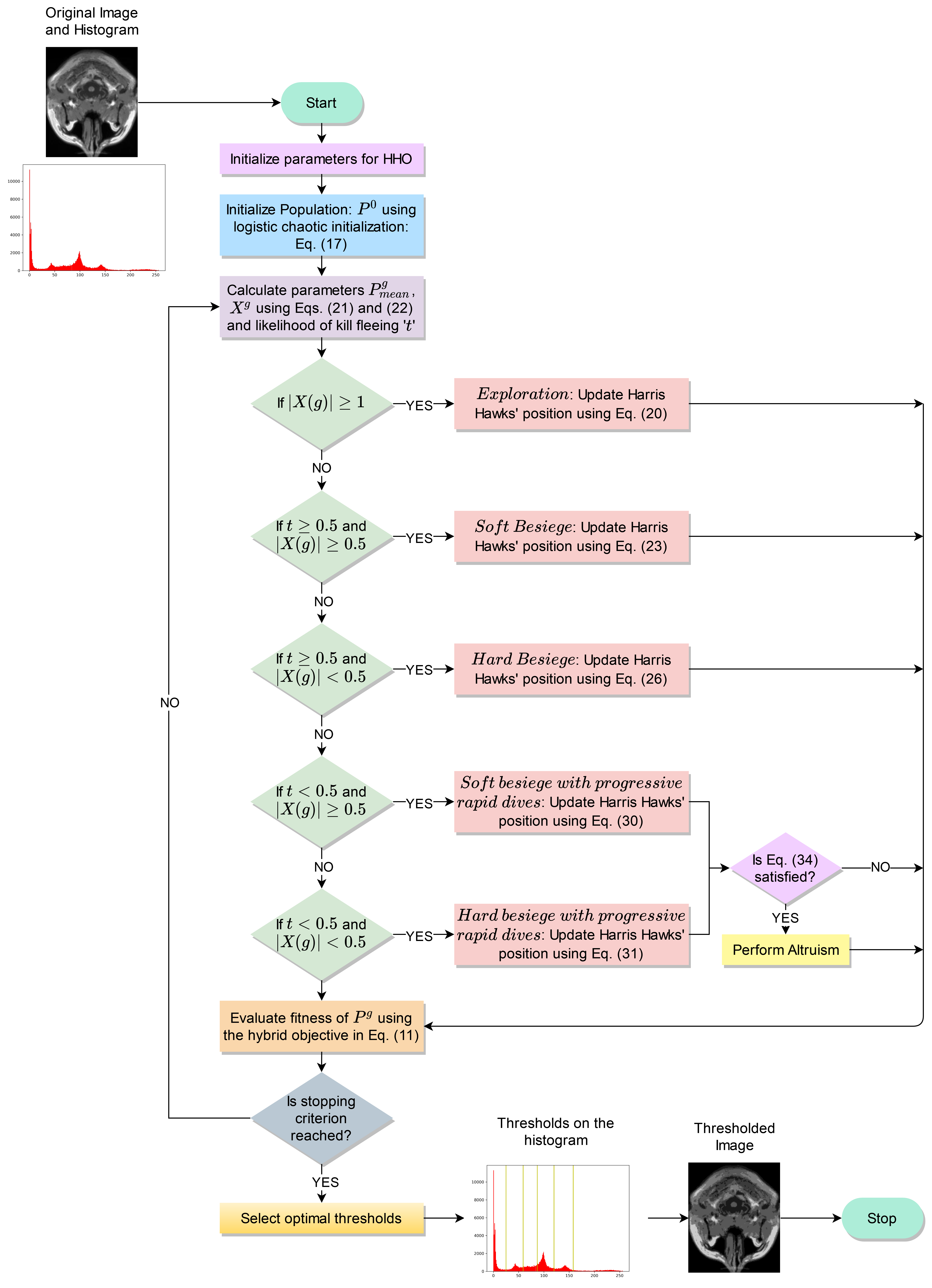
Figure 1: Flowchart of the proposed improved HHO algorithm used in this research for brain MRI segmentation using image thresholding.

The HHO algorithm [20] is a population-based, gradient-free optimization approach. It is inspired by how Harris Hawks’ track prey in the living world. The Harris Hawks’ demonstrate a special kind of approach to hunt the prey named surprise pounce. This algorithm portrays the separate exploration and exploitation strategies of the Harris Hawks, which are affected by exploring prey, the surprise pounce or the seven kills, and finally attacking the prey in a trademark style. A thorough mathematical model is portrayed to recreate how Harris Hawks’ perform hunting in nature. The myriad moves that this algorithm consists of, to imitate the pouncing technique of Harris Hawks’ are stated hereafter considering the problem of brain MRI segmentation. The flowchart of the proposed improved HHO algorithm used in this study is shown in Figure 1.

3.1 Initialization: Chaotic Map

Each of the Harris Hawks is denoted by a feature vector. The dimension of each of the Harris Hawks is equal to one added to the number of thresholds that are selected for the process of segmentation. For the first feature vector, the initialization is done randomly given that those elements of the feature vector are assigned values within the pixel range of the grayscale images. For the other vectors, the initialization is done using chaotic maps [18, 29] and it is ensured that the values lie in the pixel range of the grayscale images as before. A chaotic map is used while doing so. The other parameters are initialized to some starting value after tuning.

During chaotic initialization, let $f_{v}$ be the representation of the $v^{th}$ feature vector. So, the formulae for deriving $f_{v+1}$, the representation of the $(v+1)^{th}$ feature vector, if the value of the $v^{th}$ feature vector is given by the following:

1. Sine Chaotic Map:

   $$f_{v+1}=\frac{k}{4}sin(\pi f_{v})\,,\,k=4$$ (12)

2. Singer Chaotic Map:

   $$f_{v+1}=\mu(7.86f_{v}-23.31{f_{v}}^{2}+28.75f_{v}^{3}-13.302875f_{v}^{4})$$ (13)

   $$\mu=1.07$$

3. Sinusoidal Chaotic Map:

   $$f_{v+1}=cf_{v}^{2}sin(\pi f_{v})\,,\,c=2.3$$ (14)

4. Chebyshev Chaotic Map:

   $$f_{v+1}=cos(\arccos{f_{v}})$$ (15)

5. Tent Chaotic Map:

   $$f_{v+1}=\begin{cases}\frac{f_{v}}{0.7}&f_{v}<0.7\\ \frac{10}{3}(1-f_{v})&f_{v}\geq 0.7\end{cases}$$ (16)

6. Logistic Chaotic Map:

   $$f_{v+1}=cf_{v}(1-f_{v})\,,\,c=4$$ (17)

7. Iterative Chaotic Map:

   $$f_{v+1}=sin(\frac{c\pi}{f_{v}})\,,\,c=0.7$$ (18)

8. Gauss/Mouse Chaotic Map:

   $$f_{v+1}=e^{-\alpha f_{v}^{2}}+\beta,\alpha=4.90,\beta=-0.58$$ (19)

The method of chaotic initialization is dynamic. It is one of the most modern methods to search for the global optimum solution in a search space. The choice of a particular chaotic map has been justified in Table 3 and its corresponding reference in the results section.

3.2 Exploration

The Harris Hawks are one of the most clever and sharp birds and can strategically track down a target with their keen eyes and astute moves. The exploration is a phase of the HHO algorithm, where each of the Harris Hawks is considered a viable solution to the problem of identifying thresholds to optimize the value returned by the cost function when that particular feature vector is passed. From the current set of Harris Hawks, the prey is selected to be the one that yields the least value when passed to the objective function (the best solution among the present set of solutions is the one with minimum fitness value). To mimic the exploration phase of the Harris Hawks, there exist two plausible ways.

$$P(g+1)=\begin{cases}P_{rand}(g)-e_{1}|P_{rand}(g)-2e_{2}P(g)|,\\ when\;r\geq 0.5\\ (P_{prey}(g)-P_{mean}(g))-e_{3}(LL+e_{4}(UL-LL)),\\ when\;r<0.5\end{cases}$$ (20)

In Equation 20, $P(g)$ stands for the position of the Harris Hawk in the $g^{th}$ iteration (or generation), where $g=\{1,2,\ldots,g_{max}\}$, ‘$g_{max}$’ being the maximum number of generations. $P(g+1)$ signifies the location of the Harris Hawk at the end of the $g^{th}$ iteration. The place where the prey is located is designated by $P_{prey}(g)$. $P_{rand}(g)$ is a haphazard solution selected from the present set of Harris Hawks. Also, $r$, $e_{1},e_{2},e_{3},e_{4}$ are randomly selected values within the range (0, 1). $LL$ and $UL$ designate the lower bound and the upper bound respectively of the solutions. $P_{mean}$ is used to represent the mean or average position of the present set of Harris Hawks. $P_{mean}(i)$ is given by Equation 21.

$$P_{mean}(g)=\frac{1}{M}\sum^{M}_{j=1}P_{j}(g)$$ (21)

In Equation 21, $M$ stands for the size of the present generation of Harris Hawks and the location of the $j^{th}$ Harris Hawk in the $g^{th}$ iteration is denoted by $P_{j}(g)$.

The former viewpoint generates solutions to the image segmentation problem based on the arbitrarily selected Harris Hawks’ position as well as the position of the present set of Harris Hawks. The latter gives rise to solutions depending on the target’s location, the average or mean location of the set of Harris Hawks at the beginning of the present iteration and some factors which are randomly scaled between 0 and 1. Among these, $e_{3}$ acts as a scaling factor. As $e_{4}$ approaches 1, it increases the randomness of the method. An arbitrary length is added to the lower bound to make sure that possible solutions in the feature space are less prone to remaining undiscovered.

3.3 Changeover between Exploration and Exploitation

HHO algorithm displays a changeover between the two phases: exploration and exploitation. It also displays myriad exploitative behaviour depending on the prey’s energy to escape and its likelihood of escaping. The escaping energy of the prey goes on declining as it attempts to escape. Let’s assume that initially, the kill or the prey (the rabbit) has energy denoted by $X_{0}$, the present iteration be indicated by ‘$g$’ and the net number of iterations by ‘$g_{max}$’, then the escaping energy (say, $X(g)$) of the kill in the $g^{th}$ iteration is given by Equation 22.

$$X(g)=2X_{0}(1-\frac{g}{g_{max}})$$ (22)

$X_{0}$ lies in the scope (-1, 1) arbitrarily. As $X_{0}$ diminishes from 0 to -1, the kill gets devitalized and as $X_{0}$ increases from 0 to 1, the prey gets re-energized. Commonly, $X$ diminishes as the number of iterations increases. When $|X|\geq 1$ the algorithm goes for the exploration strategy and when $|X|<1$ the exploitation strategy is opted for.

3.4 Exploitation

In the exploitation phase, the algorithm displays the surprise pounce (or the seven kills strategy [8]) by attacking the kill detected in the phase before. But the prey tries to escape from threatening situations. So, the Harris Hawks emulate myriad chasing styles in real-life situations. The neighbourhood of the Harris Hawks is exploited in this phase. Four different approaches are manifested based on the position of the kill detected in the stage before.

The approaches are “soft besiege", “hard besiege", “soft besiege with progressive rapid dives" and “hard besiege with progressive rapid dives". The Harris Hawks choose out of soft and hard besiege approaches based on the value of ‘$X$’ as stated before, where $X$ denotes the present amount of energy left in the kill. When $|X|\geq 0.5$, it goes for soft besiege else it selects hard besiege. Another variable ‘$t$’ that denotes the likelihood of the prey escaping is taken arbitrarily in the span (0,1). A lesser value of ‘$t$’ indicates that the kill has more chances to escape. The four different approaches are described hereafter.

The algorithm chooses the soft besiege approach when $t\geq 0.5$ and $|X|\geq 0.5$. The kill has sufficient energy but it is encircled by the Harris Hawks when it attempts to mislead them and flee. Eventually, the Harris Hawks execute the surprise pounce (or the seven kills) on the prey. It can be formulated mathematically as stated in Equations 23, 24 and 25, where $P(g)$ is the population at $g^{th}$ iteration and $P(g+1)$ is the population at $(g+1)^{th}$ iteration.

$$P(g+1)=\Delta P(g)-X|JS\times P_{prey}(g)-P(g)|$$ (23)

$$\Delta P(g)=P_{prey}(g)-P(g)$$ (24)

$$JS=2(1-e_{5})$$ (25)

In these equations, $e_{5}$ is an arbitrary number in the span 0 to 1, and $JS$ stands for the kill’s arbitrary Jump Strength while it attempts to flee. $\Delta P(g)$ signifies the gap between the location of the kill and that of the present Harris Hawk in the $g^{th}$ iteration.

The algorithm goes for hard besiege when $t\geq 0.5$ and $|X|<0.5$. The prey is fatigued and it has less energy to escape the predators. The Harris Hawks hardly require to perform the surprise dive. The mathematical formulation is stated in Equation 26.

$$P(g+1)=P_{prey}(g)-X|\Delta P(g)|$$ (26)

The algorithm opts for soft besiege with continuous or progressive rapid dives if the kill possesses $|X|\geq 0.5$ and the value of $t<0.5$. The kill has sufficient energy to flee and a higher likelihood of running away. Harris Hawks accomplish the surprise pounce in two steps. The Harris Hawks encircle the kill and move to a new location after estimating the following movement of the kill (denoted by ‘$K$’) emulating the formulation in Equation 27.

$$K=P_{prey}(g)-X|JS\times P_{prey}(g)-P(g)|$$ (27)

The Harris Hawks select whether to perform the pounce after juxtaposing it with the foregoing dive and the corresponding outcome. If it is gauged that performing the pounce is unreasonable, it executes non-uniform irregular plunges based on the concept of Lévy Flight (LF). The LF concept mimics the deceptive behaviour which preys manifest to get away from their predators. The Harris Hawks display rapid and uneven plunges around the kill when it endeavours to flee. Myriad real-life observations back the LF concept, for example, how animals like monkeys and sharks chase their targets [51, 58].

$$L=K+R\times levy(N)$$ (28)

In Equation 28, $R$ is an arbitrary vector of the dimensions $1\times N$, where the dimension of the solution is depicted by $N$. Also, $levy$ is the function [62] that is used to replicate the LF concept and $N$ is calculated by Equation 27. The mathematical formulation of this function is stated in Equation 29.

$$levy(x)=0.01\times\frac{v_{1}\times\sigma}{|v_{2}|^{\frac{1}{\beta}}}\;,\sigma=\left(\frac{\Gamma(1+\beta)\times\sin({\frac{\pi\beta}{2}})}{\Gamma(\frac{1+\beta}{2})\times\beta\times 2^{(\frac{\beta-1}{2})}}\right)^{1/\beta}$$ (29)

In Equation 29, $\beta$ is initialized to 1.5. Variables $v_{1}\;and\;v_{2}$ are arbitrarily generated in the span 0 to 1, both limits are inclusive. In this approach, the location of the Harris Hawk at the close of this iteration can be updated following the mathematical formulation given in Equation 30.

$$P(g+1)=\begin{cases}K,\text{ if }fitness(K)<fitness(P(g))\\ L,\text{ if }fitness(L)<fitness(P(g))\end{cases}$$ (30)

In Equation 30, $fitness(x)$ depicts the value returned when x is passed as parameter to the fitness function.

The algorithm picks the hard besiege with continuous rapid dives when $t<0.5\;and\;|X|<0.5$. The kill does not have sufficient energy left in it to flee. The predators, the Harris Hawks, exhibit swift plunges before manifesting the surprise pounce on the kill. The new position of the Harris Hawks can be formulated mathematically as in Equation 31.

$$P(g+1)=\begin{cases}K,\text{ if }fitness(K)<fitness(P(g))\\ L,\text{ if }fitness(L)<fitness(P(g))\end{cases}$$ (31)

Here, $K$ and $L$ are obtained from the equations noted in Equations 32 and 33.

$$K=P_{prey}(g)-X|JS\times P_{prey}(g)-P_{mean}(g)|$$ (32)

$$L=K+R\times levy(N)$$ (33)

Here, $P_{mean}(g)$ is obtained as stated in Equation 21.

3.5 Altruism in HHO

Altruism [55] is a virtue that benefits other individuals at a cost to oneself. It is a state with the noble aim of increasing the welfare of another even at the cost of sacrificing its own. In the field of biology [43], it is the behaviour that increments the fitness of an individual while decrementing the fitness of the other participants. The virtue of altruism is generally observed in kin relations such as among the family members (for instance, from parent to child) but it has also been observed in larger social groups (for example, in social insects). In biology, the cost and benefit of altruism are measured in terms of reproductive fitness or the anticipated number of offspring. An individual thus reduces the number of children it is likely to give rise to and enhances the probability of another individual producing an offspring. In a gene pool, altruism evolves if the potential donor can compensate for its loss of offspring by enhancing the population by some other number of offspring having some fraction of its genes.

In the case of the HHO, each of the Harris Hawks is considered a feasible solution to the segmentation problem. The exploitation phase of HHO comprises four phases. In the latter two phases, when a Harris Hawk exhibits the progressive rapid dives, altruism has been incorporated. In each of the two cases, the feature vectors which are derived from the original feature vector are considered viable solutions. The original feature vector behaves as the altruist and the derived ones as beneficiaries. A Harris Hawk shows an altruistic nature in this case by decrementing or incrementing the value at each position by a random amount generated such that it is in between the pixel ranges of grayscale images. Similarly, for the beneficiary Harris Hawk, the value at every position is incremented or decremented respectively by the same amount with which it is decremented or incremented for the altruist provided it lies within the pixel ranges of grayscale images for the operation. Altruism is performed if Equation 34 is satisfied.

$$r\times B^{\prime}>C^{\prime}$$ (34)

Equation 34 is known as Hamilton’s rule [59]. Here, $B^{\prime}$ is the benefit or the decrease in fitness of the derived feature vector in this case. $C^{\prime}$ stands for the cost or increase in fitness of the potential altruist or the original feature vector. Also, $r$ is the relatedness of the altruist to the beneficiary or the factor by which the latter depends on the former. If this equation is not obeyed or the benefit of the recipient is less than zero, there is no altruism and the feature vectors are reverted to their earlier values.

3.6 Proposed algorithm

The proposed method wherein the HHO algorithm is combined with chaotic map initialization and altruism is shown in Algorithm 1. It is ensured that the values of the feature vectors are unique throughout the process. The uniqueness is checked while initialising the vectors, as well as, whenever one of the values of the feature vector gets updated, it is checked with other values inside the feature vector to ensure it is distinct, else that possible solution of the feature vector is discarded since the threshold values should be discrete for a particular feature vector.

3.7 Computational Complexity

The algorithm for the procedure of thresholding is HHO along with altruism. Let the number of initial features vectors be V. The computational complexity for the process of initialization will be $O(V)$. If the number of iterations is ‘$g_{max}$’ and the dimension of the search space is $N$, then the complexity for the process of updating the position of each vector is $O(V\times g_{max})+O(V\times g_{max}\times N)$ for the HHO algorithm. This is also the lower bound of the computational complexity of the algorithm since it is possible that the algorithm does not opt for either soft besiege with progressive rapid dives or hard besiege with progressive rapid dives in the exploitation phase throughout the iterations owing to probabilistic constraints. For altruism, the computational complexity is $O(g_{max}\times V\times g_{Altr}\times N)$, where $g_{Altr}$ is the number of iterations taking place in the function for altruism. For the thresholding process, the upper bound of the computational complexity, hence, is $O(V+V\times g_{max}(1+N)+g_{max}\times V\times g_{Altr}\times N)$.

Algorithm 1 The Pseudo-code for HHO with chaotic initialization and altruism

Input: Population size ‘$M$’ and maximum number of iterations ‘$g_{max}$’
Output: Location of the kill and the value obtained when it is passed as parameter to the fitness function

  Set the values of the first Harris Hawk randomly

  Set the remaining Harris Hawks by applying the Logistic chaotic map - using Equation 17

  for $g$ in {$1$ to $g_{max}$} do

     Determine the fitness values of the Harris Hawks by passing the particular feature vector as parameter to the fitness function

     The Harris Hawk with best fitness value is set to be the prey, denoted by $P_{prey}(g)$

     for each Harris Hawk do

        For the exploitation phase, set Jump Strength (JS): $JS=2(1-rand())$

        Determine the present energy X using Equation 21

        if $|X(g)|\geq 1$ then

           Perform exploration following Equation 20 and correspondingly, update the Harris Hawk’s position

        else if $|X(g)|<1$ then

           Say, X and t stand for the present energy of the kill and likelihood of the kill fleeing, respectively

           if $t\geq 0.5$ and $|X(g)|\geq 0.5$ then

              Opt for Soft besiege in accordance with equations 23 to 25 and update position of the Harris Hawk

           else if $t\geq 0.5$ and $|X(g)|<0.5$ then

              Opt for Hard besiege in accordance with Equation 26 and update position of the Harris Hawk

           else if $t<0.5$ and $|X(g)|\geq 0.5$ then

              Opt for Soft besiege with progressive rapid dives in accordance with Equations 27 to 30 and update position of the Harris Hawk and similarly check for Altruism in each of the derived feature vectors from the original Harris Hawk such that Equation 34 is obeyed

           else if $t<0.5$ and $|X(g)|<0.5$ then

              Opt for Hard besiege with progressive rapid dives in accordance with Equations 31 to 33 and update position of the Harris Hawk and check for Altruism in each of the derived feature vectors from the original Harris Hawk such that Equation 34 is obeyed.

           end if

        end if

     end for

     if Fitness of best solution == Concluding Condition then

        Break out of the for loop

     end if

  end for

  Return the best solution along with the value obtained when it is passed as a parameter to the fitness function

4 Results and Discussion

In this section, we describe the datasets used in this research and the evaluation outcomes of the proposed model on these datasets. Further, we discuss the implications of the results obtained and compare the proposed model to state-of-the-art methods and establish the reliability of the approach.

4.1 Datasets Used

The proposed method has been evaluated on two datasets: (1) Ten T2-weighted images via magnetic resonance transaxial cut brain obtained from the WBA database developed by the Harvard Medical School [56] and (2) Eight benchmark MRIs extracted from Brainweb database [13].

4.2 Evaluation Metrics

To evaluate the performance of the proposed method the following six popularly used metrics have been considered:

1. Peak Signal to Noise Ratio (PSNR) [6]: The mathematical formula for PSNR is given in Equation 35, where $Max_{I}$ is the maximum pixel value of image $I$ and $MSE$ denotes the Mean Squared Error.

   $$PSNR=10\log_{10}\left(\frac{Max_{I}^{2}}{MSE}\right)$$ (35)

2. Structural Similarity Index (SSIM) [61]: The SSIM is calculated using Equation 36 between two images (say $I_{a}$ and $I_{b}$).

   $$SSIM(I_{a},I_{b})=\frac{(2\mu_{I_{a}}\mu_{I_{b}}+c_{1})\times(2\sigma_{I_{a}I_{b}})}{(\mu_{I_{a}}^{2}+\mu_{I_{b}}^{2}+c_{1})\times(\sigma_{I_{a}}^{2}+\sigma_{I_{b}}^{2}+c_{2})}$$ (36)

   where, $\mu$ and $\sigma$ are the mean and standard deviations of pixel values of the images, $\sigma_{I_{a}I_{b}}$ is the covariance of $I_{a}$ and $I_{b}$, and $c_{1}$ and $c_{2}$ are two variables for weak denominator stabilization.

3. Feature Similarity Index (FSIM) [64]: Mathematically, the FSIM metric is formulated as in Equation 37, where, $S_{L}(x)$ denotes the overall similarity between two images $I_{a}$ and $I_{b}$; $PC$ denotes the phase congruence between the images and $\Omega$ denotes the whole spatial domain of the image.

   $$FSIM=\frac{\sum_{x\in\Omega}S_{L}(x)\times PC_{m}(x)}{\sum_{x\in\Omega}PC_{m}(x)}$$ (37)

4. Haar wavelet-based Perceptual Similarity Index (HPSI) [48]: The HPSI for two images $X$, $Y$ is given as Equation 38.

   $$HPSI(X,Y)=\frac{1}{l_{\alpha}}\left(\frac{\sum_{x}\sum_{k=1}^{2}HS_{X,Y}^{(k)}[x]\times W_{X,Y}^{(k)}[x]}{\sum_{x}\sum_{k=1}^{2}W_{X,Y}^{(k)}[x]}\right)^{2}$$ (38)

   where, $l_{\alpha}$ is a logistic function for a parameter $\alpha>0$ used to model the perceptual similarity; $HS$ is the local similarity measure based on Haar wavelet transform and $W_{X,Y}^{(k)}$ is a weight map given by Equation 39.

   $$W_{X,Y}^{(k)}[x]=max(W_{X}^{(k)}[x],W_{Y}^{(k)}[x])$$ (39)

5. Quality Index based on Local Variance (QILV) [2]: The QILV metric appraises the changes in the non-stationary behaviour of images and is calculated by Equation 40 between images $X$ and $Y$.

   $$QILV(X,Y)=\left(\frac{2\mu_{V_{X}}\mu_{V_{Y}}}{\mu_{V_{X}}^{2}+\mu_{V_{Y}}^{2}}\right)\times\left(\frac{2\sigma_{V_{X}}\sigma_{V_{Y}}}{\sigma_{V_{X}}^{2}+\sigma_{V_{Y}}^{2}}\right)\times\left(\frac{\sigma_{V_{X}V_{Y}}}{\sigma_{V_{X}}\sigma{V_{Y}}}\right)$$ (40)

   $\mu$ and $\sigma$ are the global mean and standard deviations of the local variances $V_{X}$ and $V_{Y}$ respectively of images $X$ and $Y$.

6. Universal Image Quality Index (UIQI) [60]: The UIQI evaluates the distortion of an image as a combination of correlation loss, luminance distortion, and contrast distortion and is calculated by Equation 41.

   $$UIQI(X,Y)=\frac{4\sigma_{XY}\mu_{X}\mu_{Y}}{(\sigma_{X}^{2}+\sigma_{Y}^{2})(\mu_{X}^{2}+\mu_{Y}^{2})}$$ (41)

   For the images $X$ and $Y$, $\mu$ and $\sigma$ denote their mean and standard deviations and $\sigma_{X}Y$ denotes the covariance of the images.

4.3 Implementation

Table 1: Results obtained on the Harvard WBA brain MRI dataset where the number of the slice is mentioned.

Slice	No. of Thresholds	PSNR	SSIM	FSIM	UIQI	QILV	HPSI	Time(s)
22	2	23.1170	0.8175	0.7964	0.4396	0.7452	0.6905	22.6105
	3	24.8599	0.8656	0.8622	0.5448	0.8396	0.7912	26.8900
	4	26.3159	0.8956	0.8961	0.6211	0.8917	0.8389	30.6944
	5	27.6278	0.9146	0.9232	0.6752	0.9246	0.8784	34.4573
32	2	22.5471	0.8239	0.8025	0.4308	0.7302	0.6808	23.4577
	3	24.2922	0.8698	0.8625	0.5517	0.8348	0.7869	27.6399
	4	25.7215	0.8943	0.8991	0.6140	0.8867	0.8399	31.2163
	5	26.9763	0.9183	0.9239	0.6784	0.9137	0.8808	35.2593
42	2	21.7223	0.8148	0.8098	0.4277	0.7197	0.6542	23.1100
	3	23.2718	0.8550	0.8519	0.5065	0.8180	0.7519	27.5122
	4	24.7889	0.8865	0.8884	0.5750	0.8749	0.8130	31.4134
	5	25.9590	0.9013	0.9120	0.6168	0.9115	0.8532	35.9043
52	2	21.7282	0.8242	0.8024	0.4698	0.7663	0.6601	22.6908
	3	23.7954	0.8802	0.8635	0.5540	0.8304	0.7739	27.4299
	4	25.0807	0.9011	0.8964	0.6188	0.8873	0.8275	31.5897
	5	26.0764	0.9168	0.9124	0.6730	0.9156	0.8595	35.2184
62	2	20.4246	0.7986	0.7597	0.4108	0.7426	0.5920	23.2198
	3	22.6551	0.8587	0.8229	0.5106	0.8108	0.7063	27.4539
	4	24.1148	0.8882	0.8593	0.5747	0.8765	0.7788	31.1962
	5	25.4218	0.9085	0.8910	0.6403	0.9136	0.8341	35.5530
72	2	19.6996	0.7935	0.7426	0.3672	0.6857	0.5737	23.0623
	3	21.8478	0.8370	0.8043	0.4747	0.8137	0.6733	27.1111
	4	24.0422	0.8891	0.8534	0.5519	0.8614	0.7711	32.4240
	5	25.3464	0.9118	0.8891	0.6214	0.9065	0.8212	36.0055
82	2	19.9938	0.8001	0.7420	0.3571	0.6513	0.5857	23.2232
	3	22.5303	0.8441	0.8081	0.4840	0.7994	0.6851	27.2413
	4	24.3912	0.8929	0.8591	0.5587	0.8414	0.7928	31.6598
	5	25.5322	0.9115	0.8935	0.6294	0.8855	0.8367	36.3615
92	2	21.1111	0.8243	0.7745	0.3936	0.7317	0.6148	23.1599
	3	23.9383	0.8822	0.8408	0.4671	0.8201	0.7396	27.5972
	4	25.7974	0.9074	0.8801	0.5743	0.8922	0.8265	31.6055
	5	26.9757	0.9194	0.9083	0.6359	0.9243	0.8608	35.6105
102	2	21.7561	0.8646	0.8454	0.4135	0.7308	0.6522	22.7122
	3	24.6831	0.9082	0.8842	0.5011	0.8255	0.7473	27.5126
	4	26.0502	0.9284	0.9173	0.5917	0.8868	0.8270	31.3697
	5	27.3213	0.9386	0.9349	0.6701	0.9236	0.8618	36.0524
112	2	24.1399	0.8948	0.9012	0.4069	0.7199	0.6601	23.4277
	3	25.8955	0.9214	0.9306	0.4962	0.8272	0.7435	27.7060
	4	27.3790	0.9382	0.9533	0.6142	0.8854	0.8294	31.5294
	5	28.8877	0.9545	0.9664	0.6740	0.9156	0.8834	37.0770

Table 2: Results obtained on the Brainweb database where the number of the image title indicates the z-plane of the analyzed image

Image	No. of Thresholds	PSNR	SSIM	FSIM	UIQI	QILV	HPSI	Time (s)
Z1	2	17.9955	0.6164	0.7138	0.2213	0.7264	0.4953	33.4307
	3	21.0102	0.7479	0.8063	0.3283	0.8204	0.7042	38.1369
	4	22.756	0.7897	0.8491	0.4104	0.8586	0.7651	43.716
	5	24.0058	0.8031	0.875	0.4352	0.92	0.8058	49.2387
Z2	2	17.9547	0.6129	0.7104	0.2168	0.7225	0.493	33.3904
	3	21.0538	0.7466	0.8049	0.3262	0.8203	0.6958	37.7423
	4	22.8181	0.7885	0.8475	0.4087	0.8599	0.7592	42.9616
	5	24.0395	0.8059	0.8758	0.4532	0.9232	0.8094	49.4712
Z5	2	18.9015	0.6563	0.7091	0.2391	0.6544	0.5286	33.3372
	3	21.0832	0.742	0.8117	0.3244	0.8088	0.7012	43.45
	4	22.9353	0.7831	0.8559	0.4081	0.8577	0.7632	48.9929
	5	24.0307	0.7956	0.8777	0.4299	0.9162	0.8058	53.3716
Z10	2	19.3314	0.6553	0.7256	0.2403	0.6215	0.5284	30.8795
	3	21.3817	0.7293	0.818	0.3179	0.7853	0.707	37.8957
	4	23.2543	0.7712	0.864	0.3943	0.8458	0.7751	42.3333
	5	24.3016	0.7916	0.8844	0.4518	0.8866	0.8022	47.4749
Z36	2	19.1749	0.7004	0.7682	0.2678	0.6464	0.5364	31.8485
	3	21.3443	0.7676	0.8396	0.3484	0.8013	0.7007	37.8283
	4	23.1914	0.8074	0.8747	0.4207	0.8582	0.7661	44.1279
	5	24.2994	0.8191	0.8953	0.4383	0.9183	0.8011	50.1885
Z72	2	20.7149	0.8165	0.8393	0.357	0.8435	0.7331	32.9571
	3	23.165	0.8626	0.8815	0.4451	0.9135	0.7991	37.2743
	4	23.6653	0.8702	0.8968	0.4541	0.9266	0.807	43.7322
	5	25.1448	0.8918	0.9179	0.5177	0.9514	0.8441	50.1932
Z108	2	21.4394	0.8398	0.8218	0.3448	0.8326	0.7452	31.6718
	3	22.0079	0.8493	0.8412	0.36	0.8612	0.7573	41.4043
	4	24.1245	0.8885	0.8882	0.4418	0.9092	0.8222	43.3232
	5	25.6447	0.9055	0.9127	0.5066	0.9387	0.8598	50.112
Z144	2	21.4795	0.8435	0.8334	0.2816	0.6312	0.5945	32.7324
	3	23.9674	0.8854	0.8909	0.3892	0.7954	0.7624	38.6617
	4	25.5294	0.9025	0.9164	0.4516	0.8637	0.8273	46.4189
	5	26.6825	0.9134	0.9285	0.5031	0.8991	0.8541	50.1067

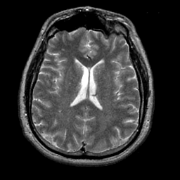
(a) Original

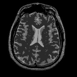
(b) 2 Thresholds

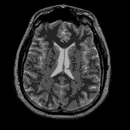
(c) 3 Thresholds

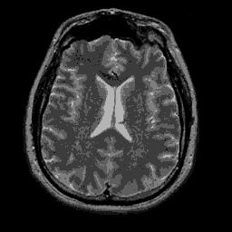
(d) 4 Thresholds

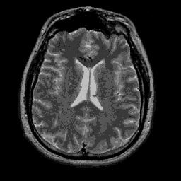
(e) 5 Thresholds

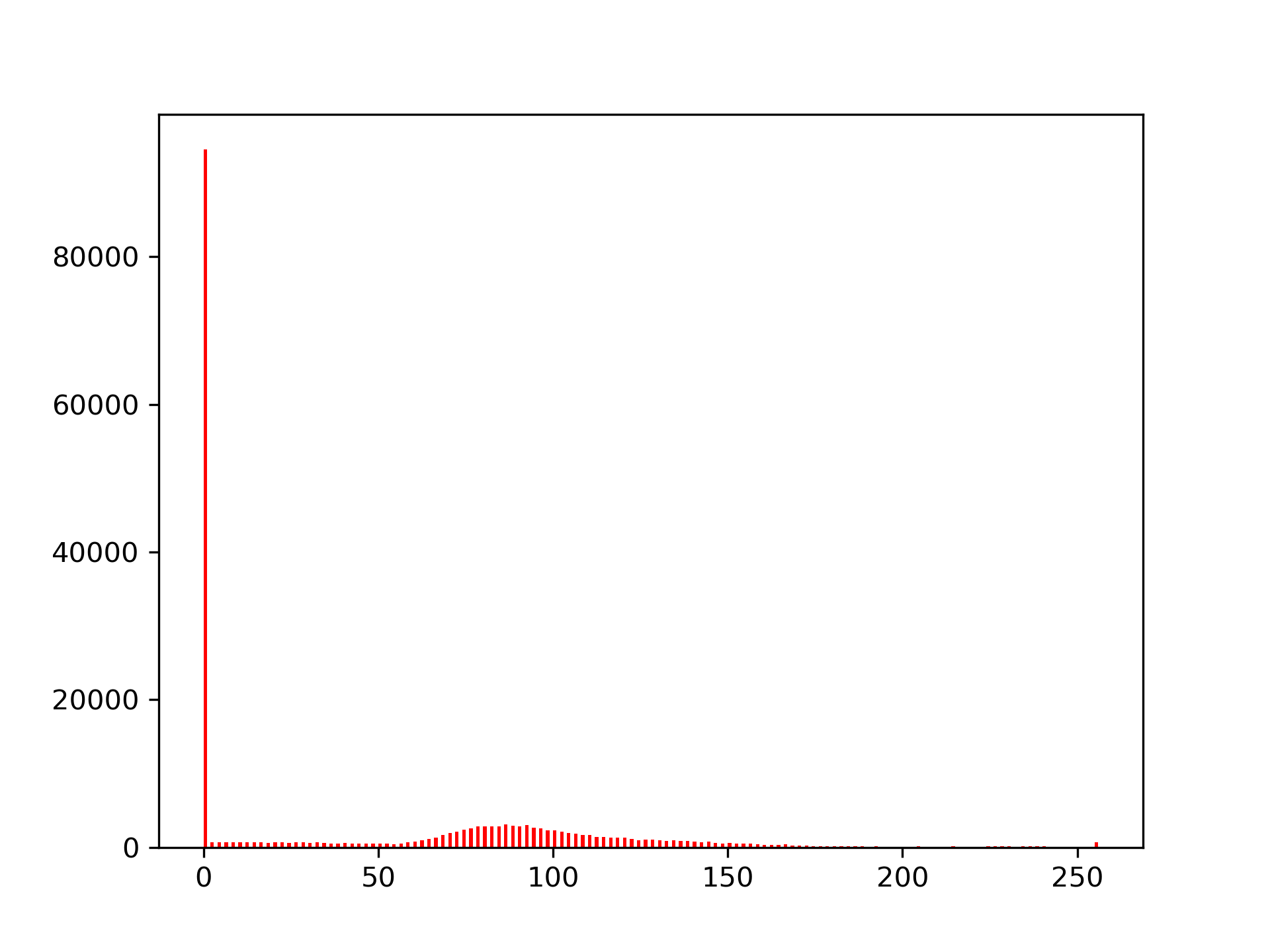
(f) Original

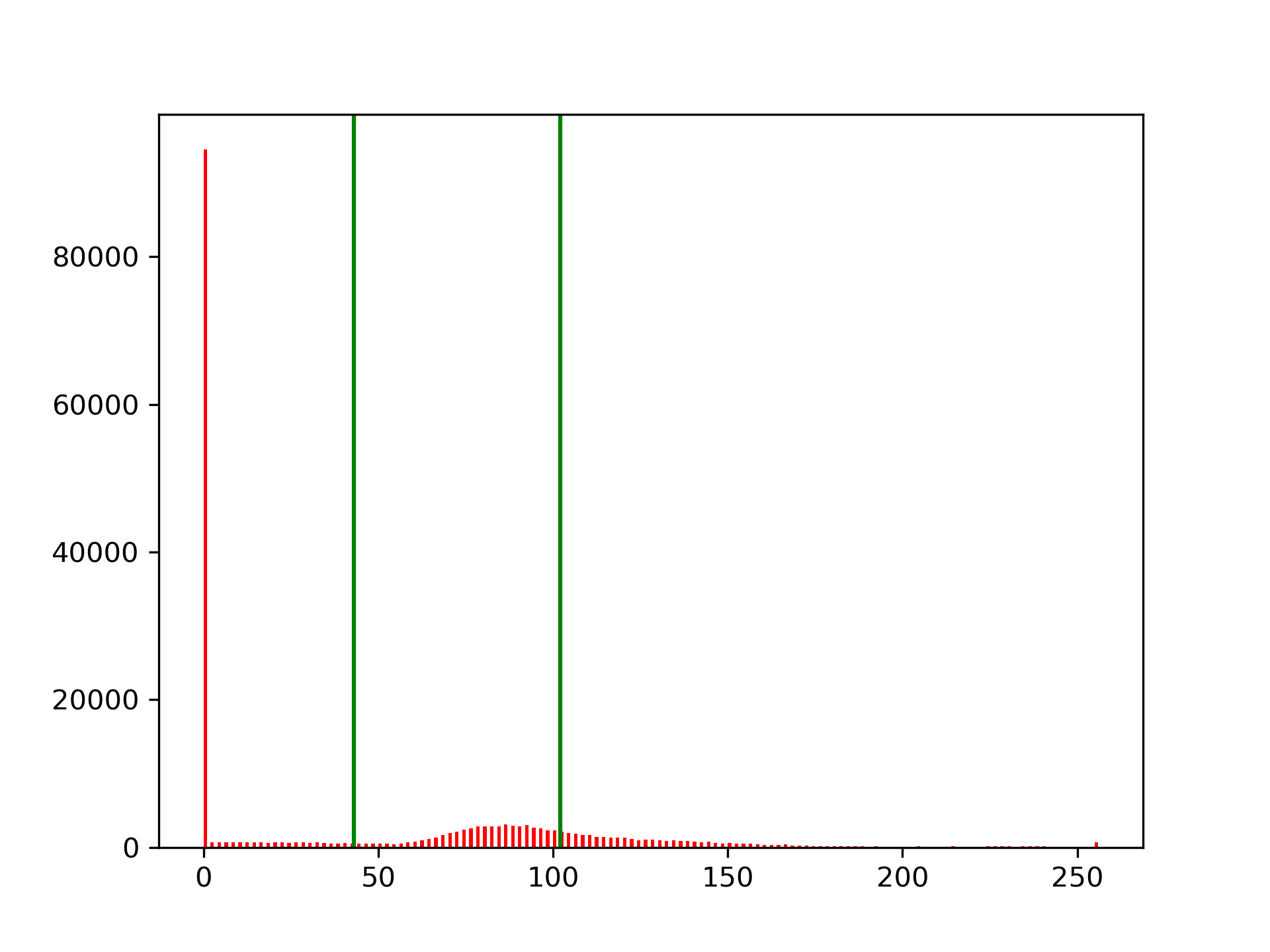
(g) 2 Thresholds

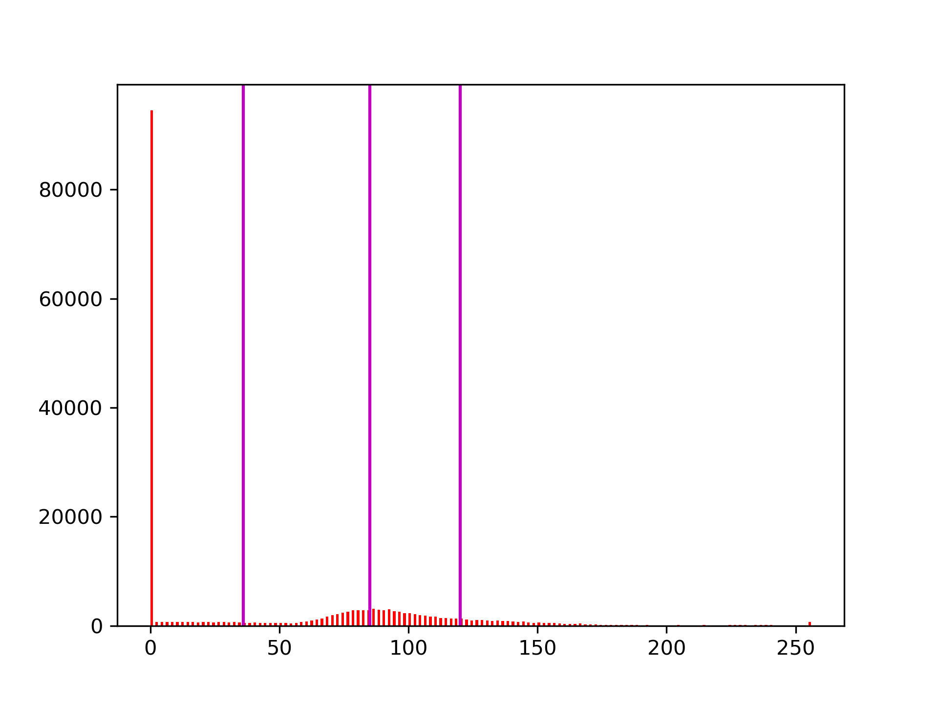
(h) 3 Thresholds

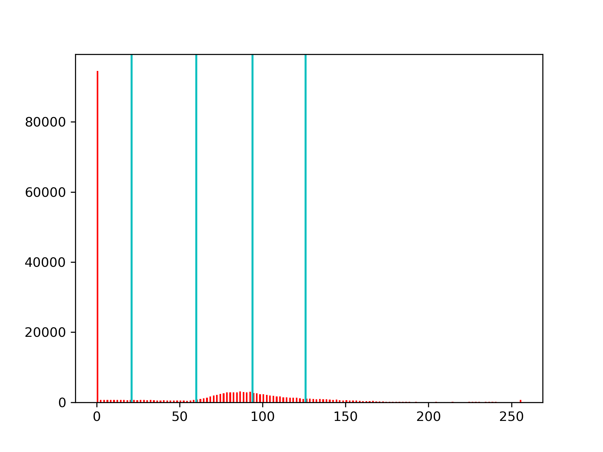
(i) 4 Thresholds

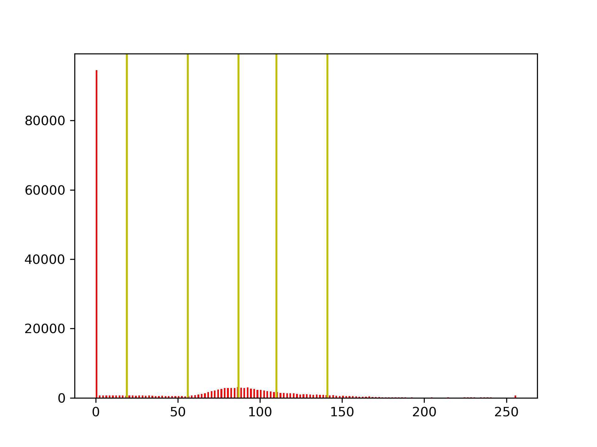
(j) 5 Thresholds

Figure 5: Original image and thresholded images for slice 82 of the Harvard WBA dataset with number of thresholds: 2, 3, 4 and 5, with their corresponding histograms and thresholds marked with vertical lines.

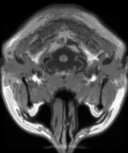
(a) Original

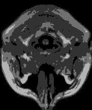
(b) 2 Thresholds

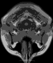
(c) 3 Thresholds

(d) 4 Thresholds

(e) 5 Thresholds

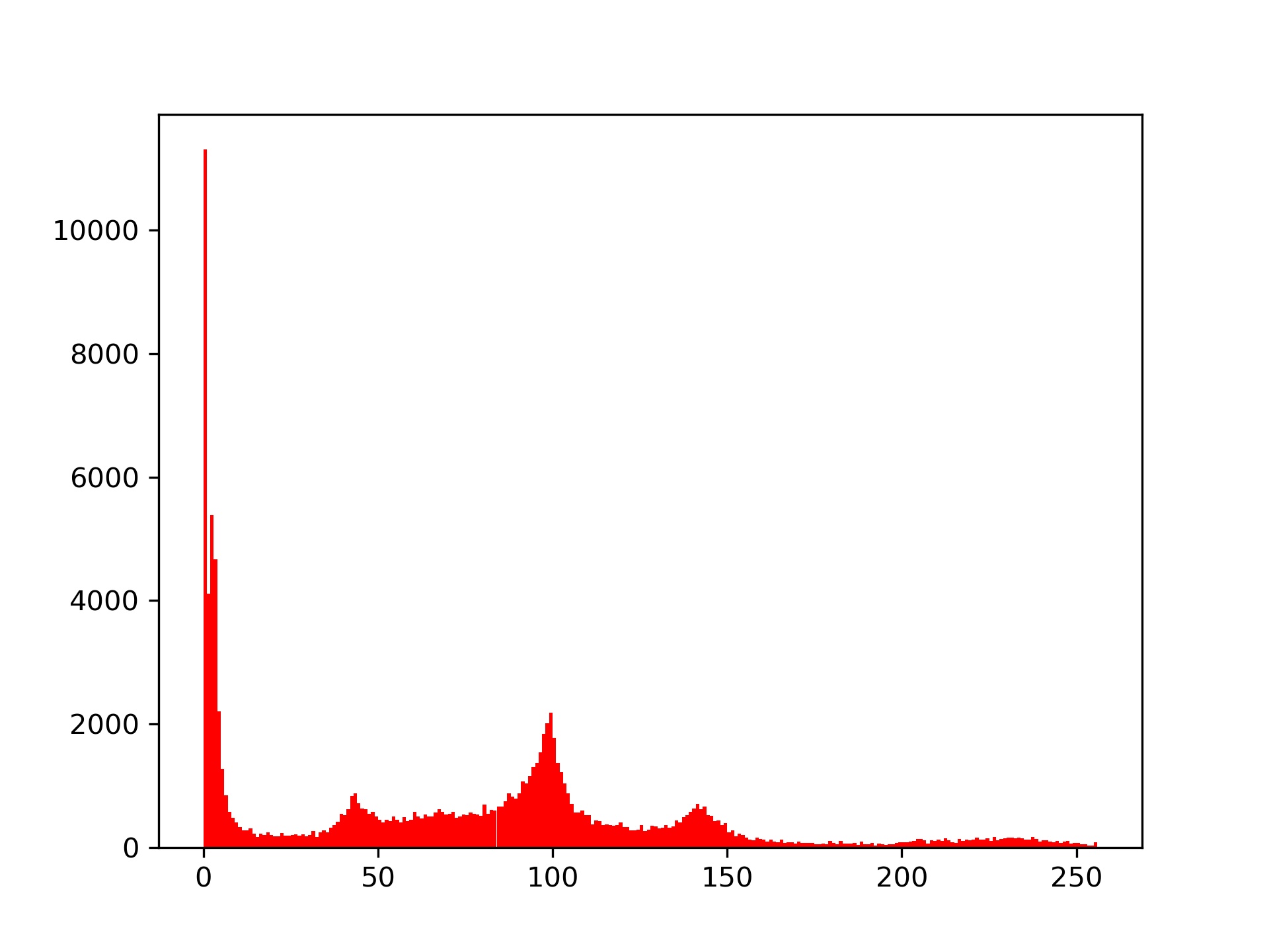
(f) Original

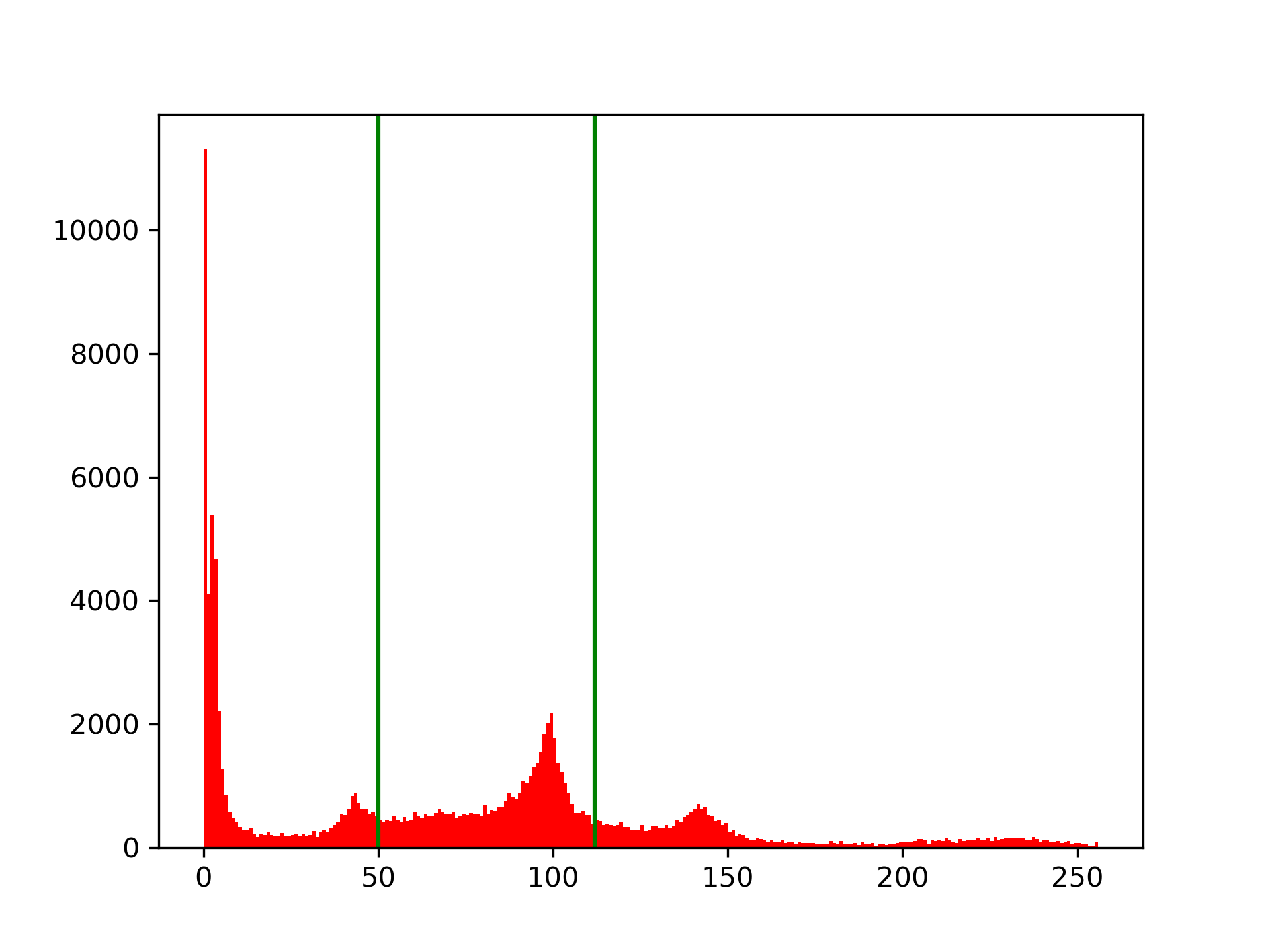
(g) 2 Thresholds

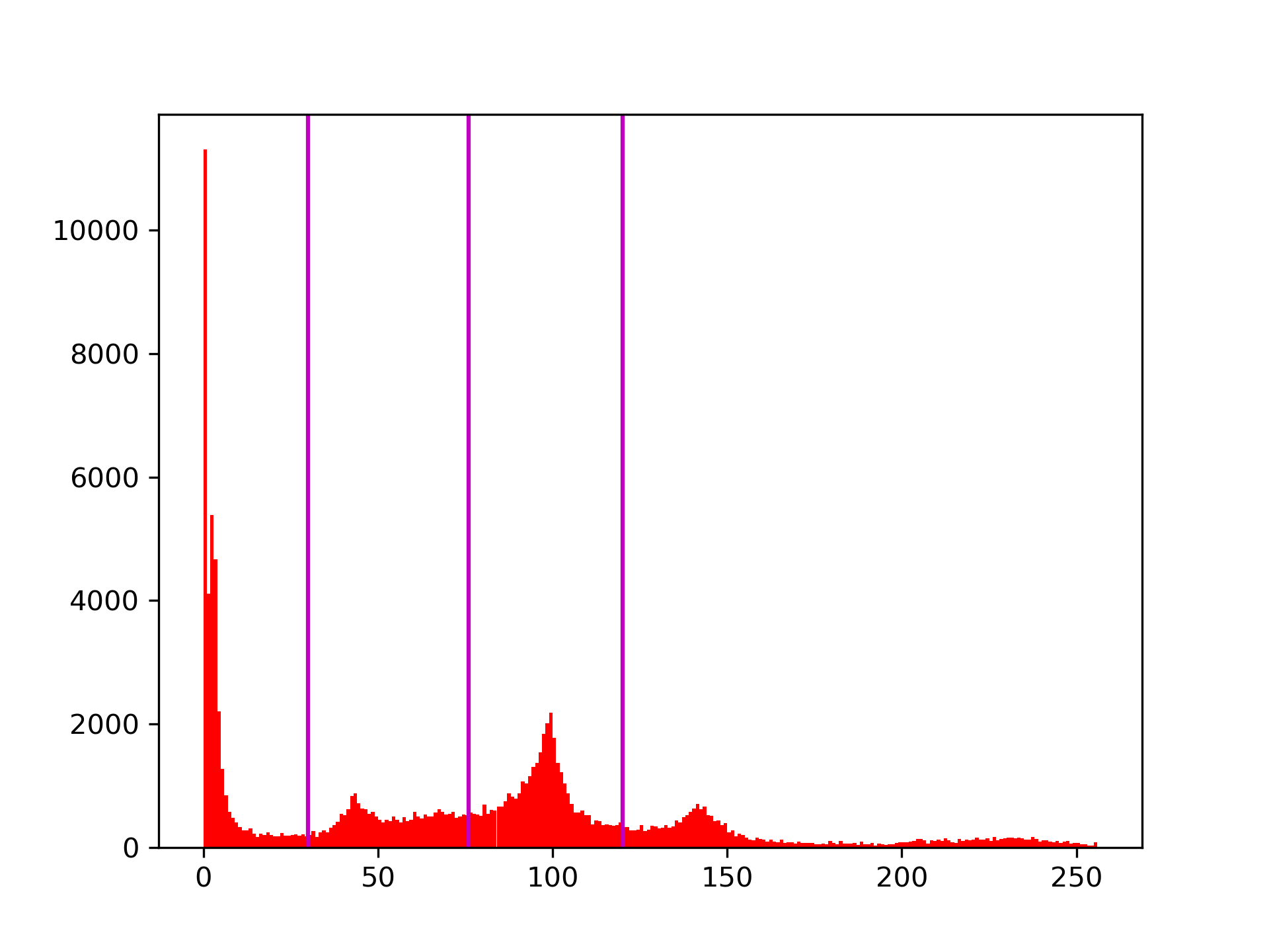
(h) 3 Thresholds

(i) 4 Thresholds

(j) 5 Thresholds

Figure 6: Original image and thresholded images for Brainweb dataset image Z1 with number of thresholds: 2, 3, 4 and 5, with their corresponding histograms and thresholds marked with vertical lines.

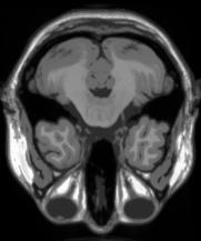
(a) Original

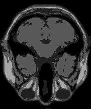
(b) 2 Thresholds

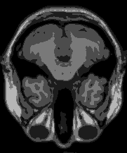
(c) 3 Thresholds

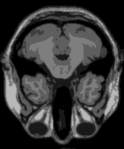
(d) 4 Thresholds

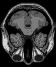
(e) 5 Thresholds

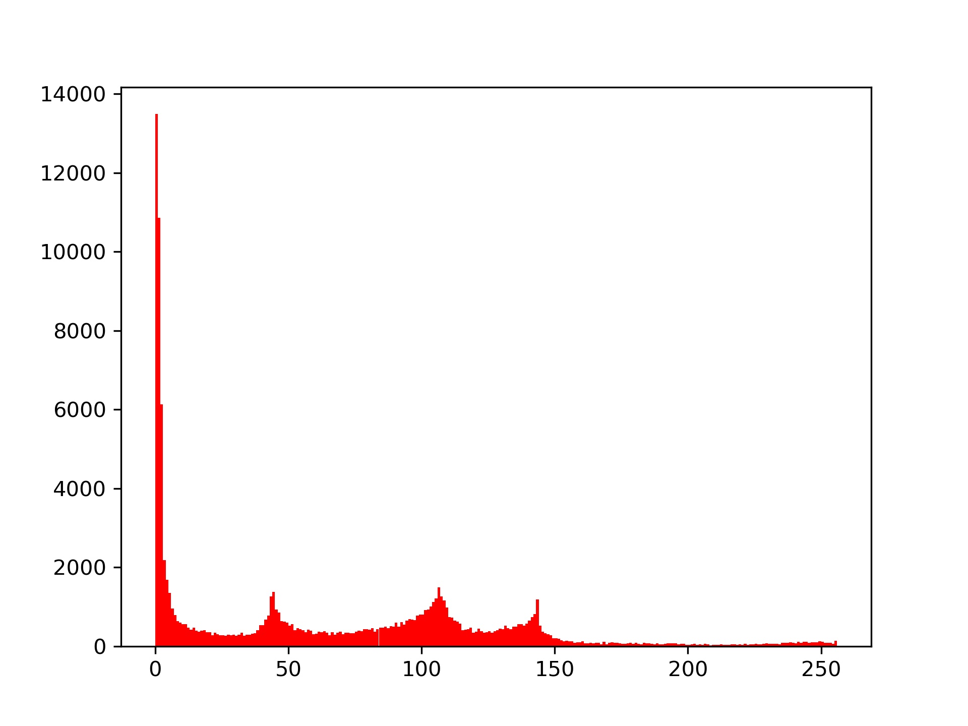
(f) Original

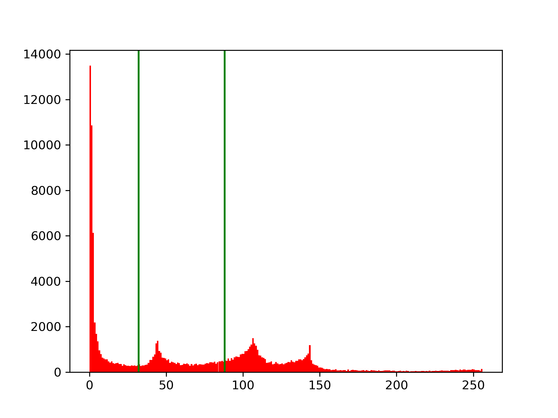
(g) 2 Thresholds

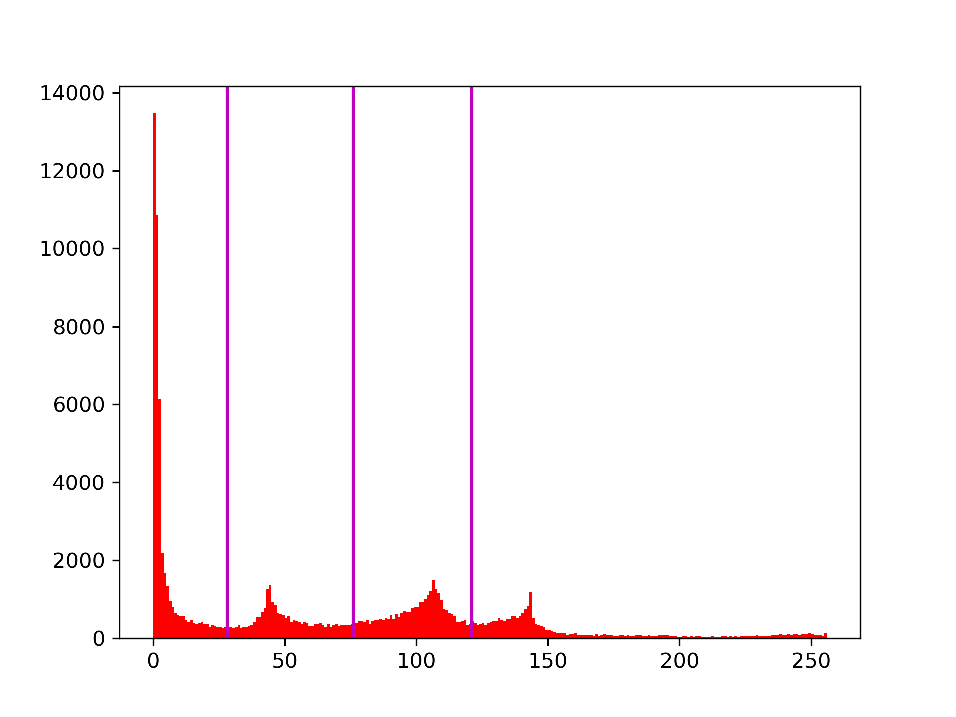
(h) 3 Thresholds

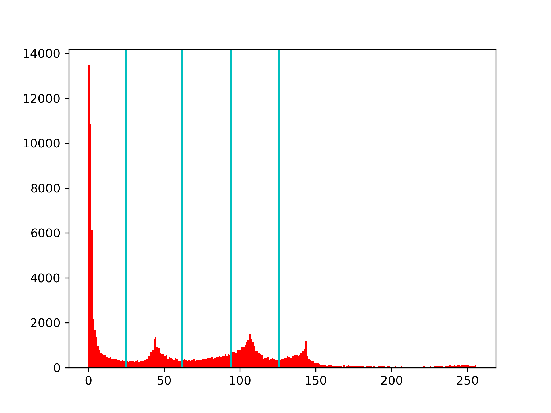
(i) 4 Thresholds

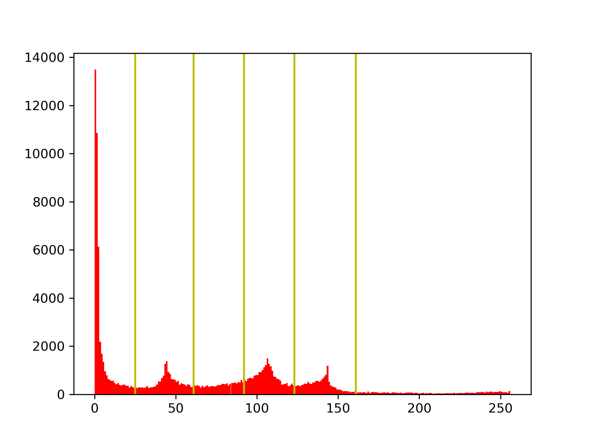
(j) 5 Thresholds

Figure 7: Original image and thresholded images for Brainweb dataset image Z36 with number of thresholds: 2, 3, 4 and 5, with their corresponding histograms and thresholds marked with vertical lines.

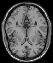
(a) Original

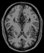
(b) 2 Thresholds

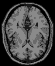
(c) 3 Thresholds

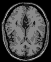
(d) 4 Thresholds

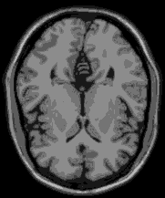
(e) 5 Thresholds

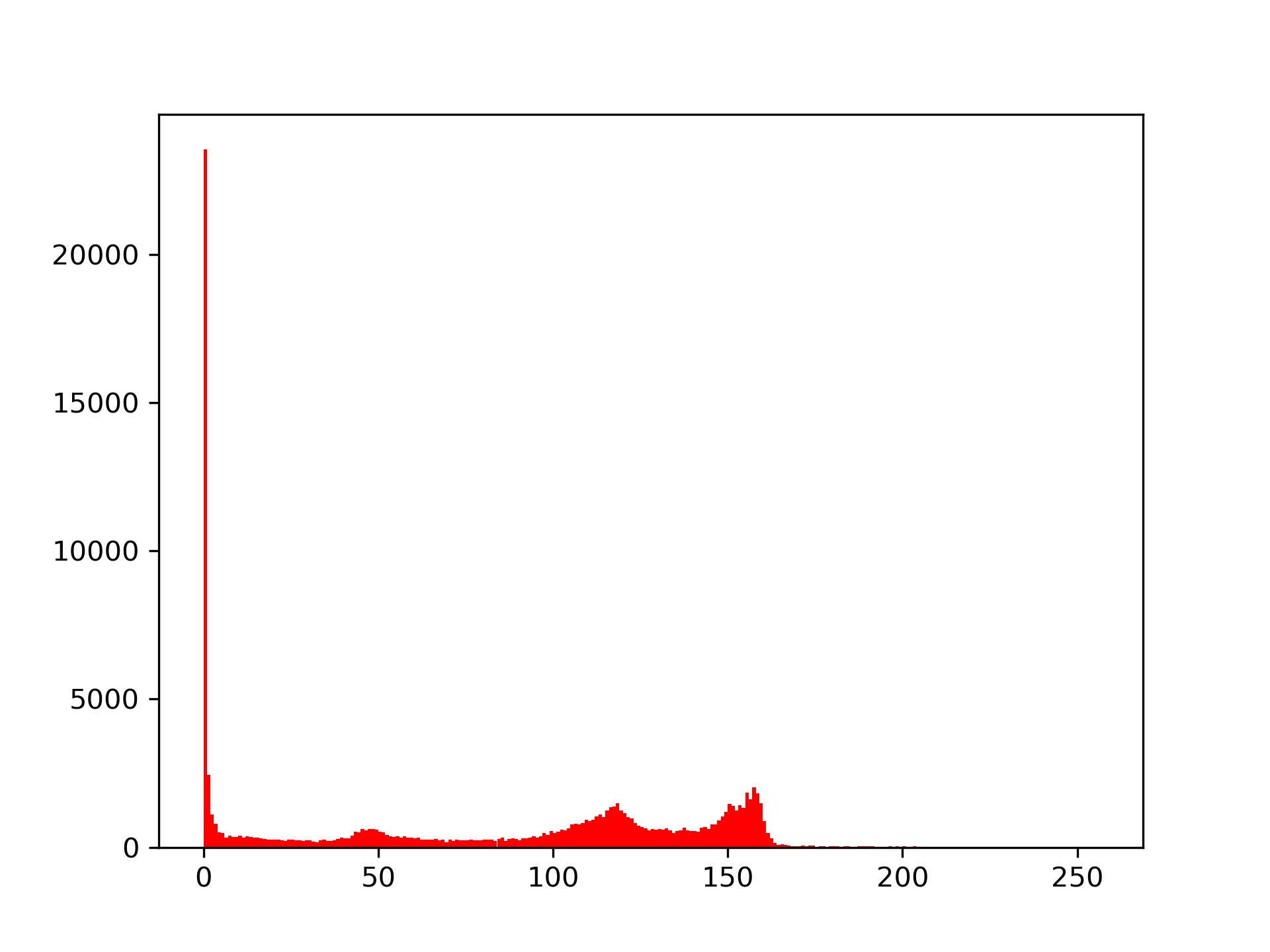
(f) Original

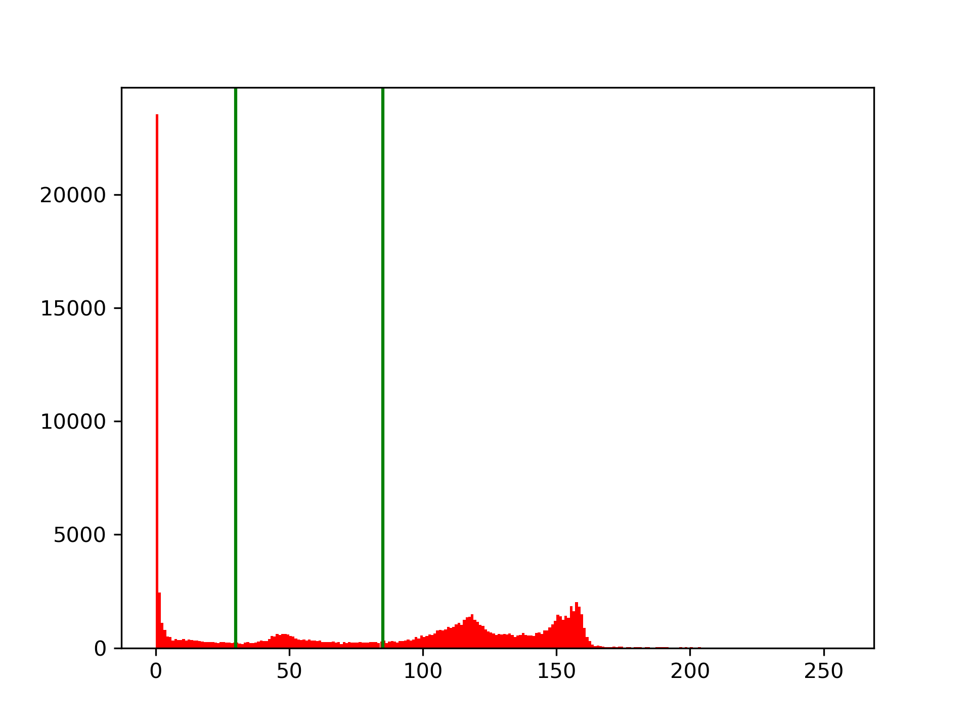
(g) 2 Thresholds

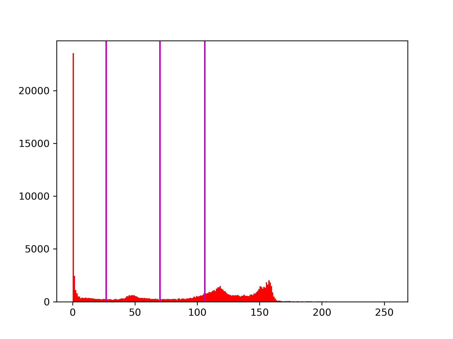
(h) 3 Thresholds

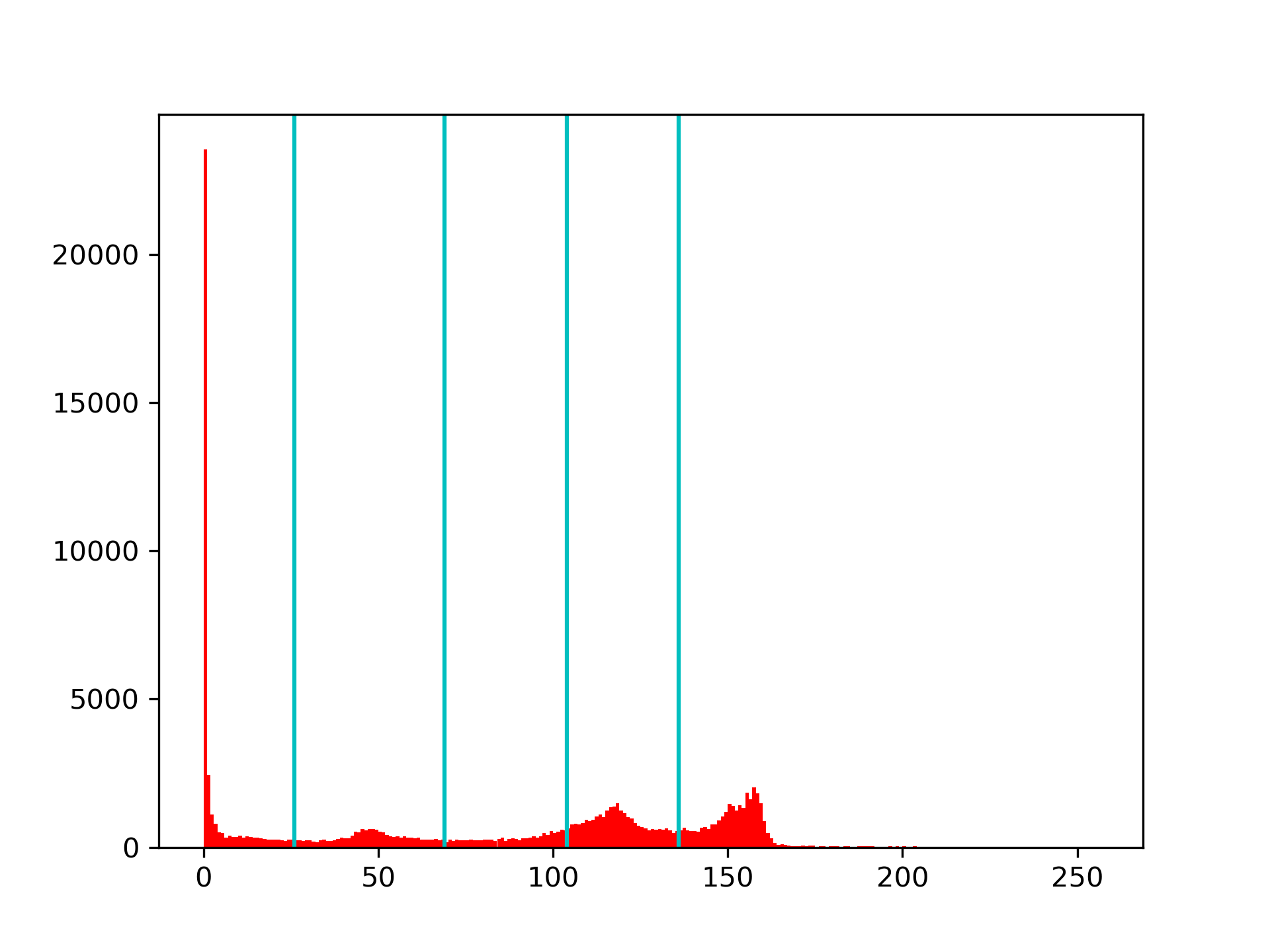
(i) 4 Thresholds

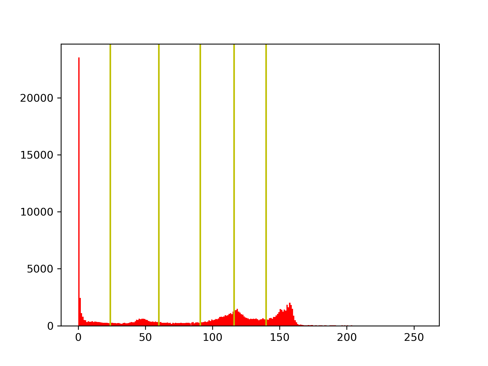
(j) 5 Thresholds

Figure 8: Original image and thresholded images for Brainweb dataset image Z72 with number of thresholds: 2, 3, 4 and 5, with their corresponding histograms and thresholds marked with vertical lines.

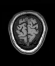
(a) Original

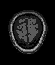
(b) 2 Thresholds

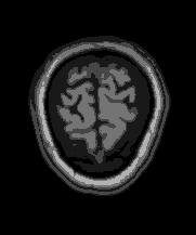
(c) 3 Thresholds

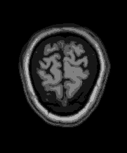
(d) 4 Thresholds

(e) 5 Thresholds

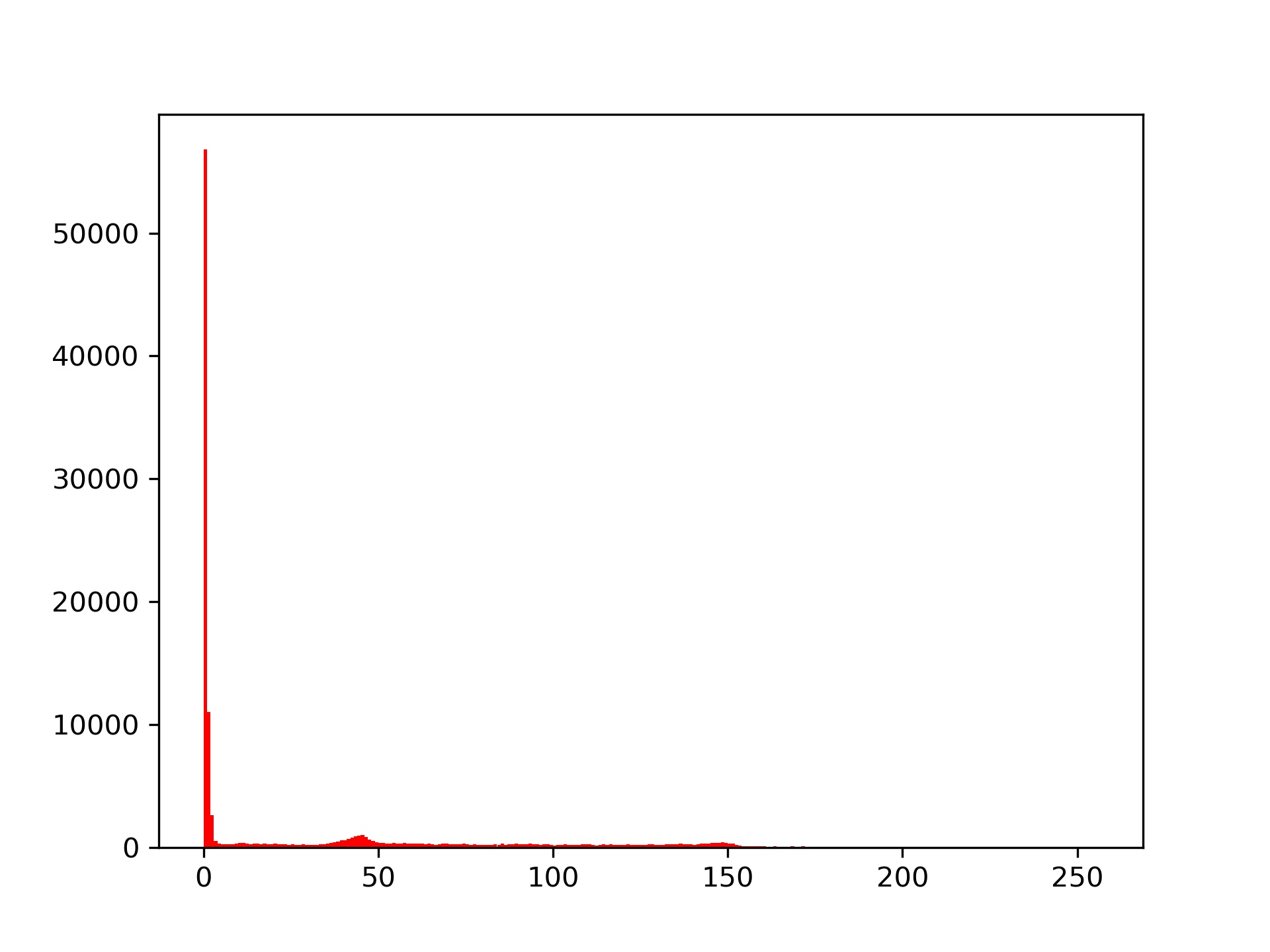
(f) Original

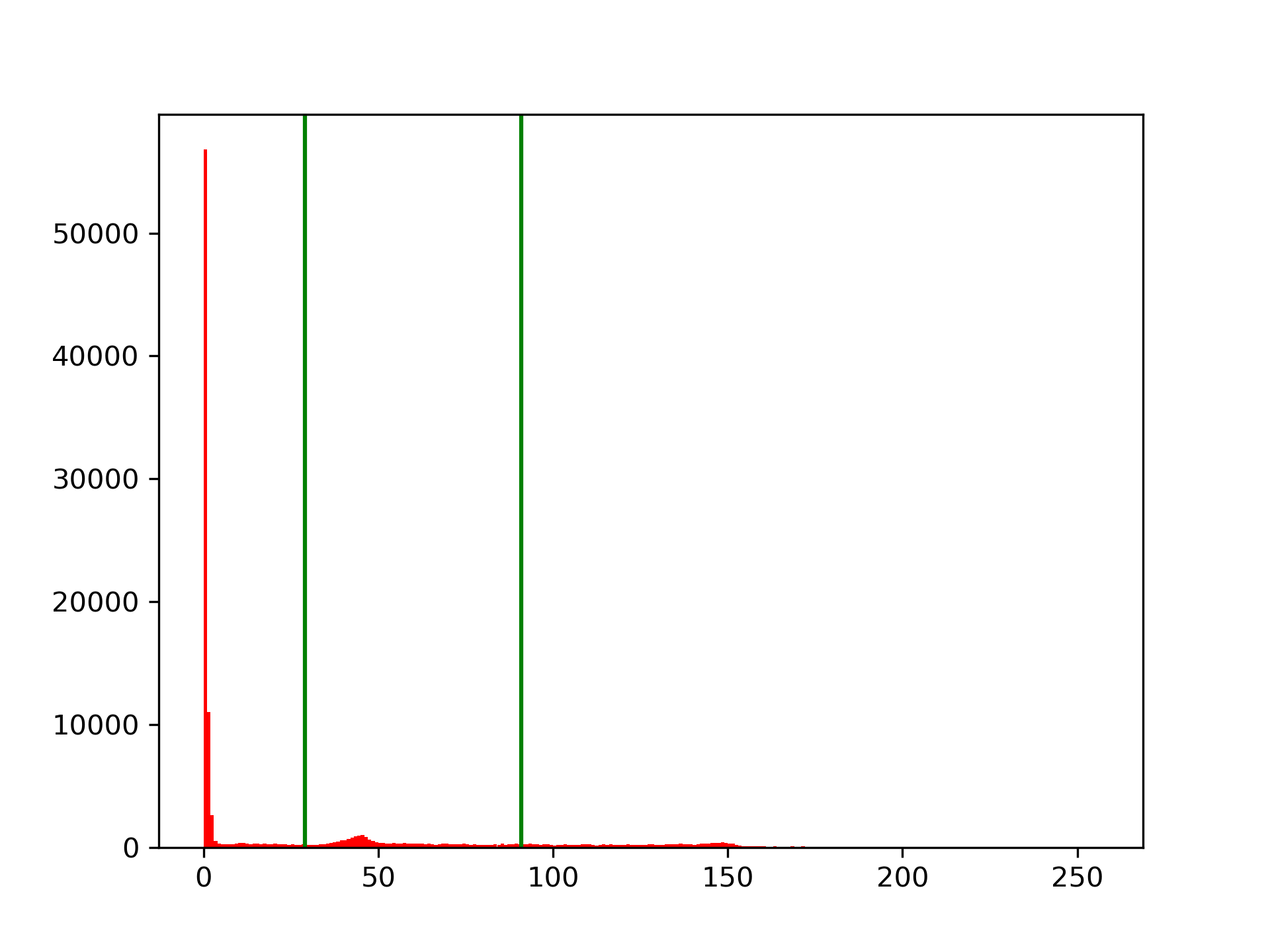
(g) 2 Thresholds

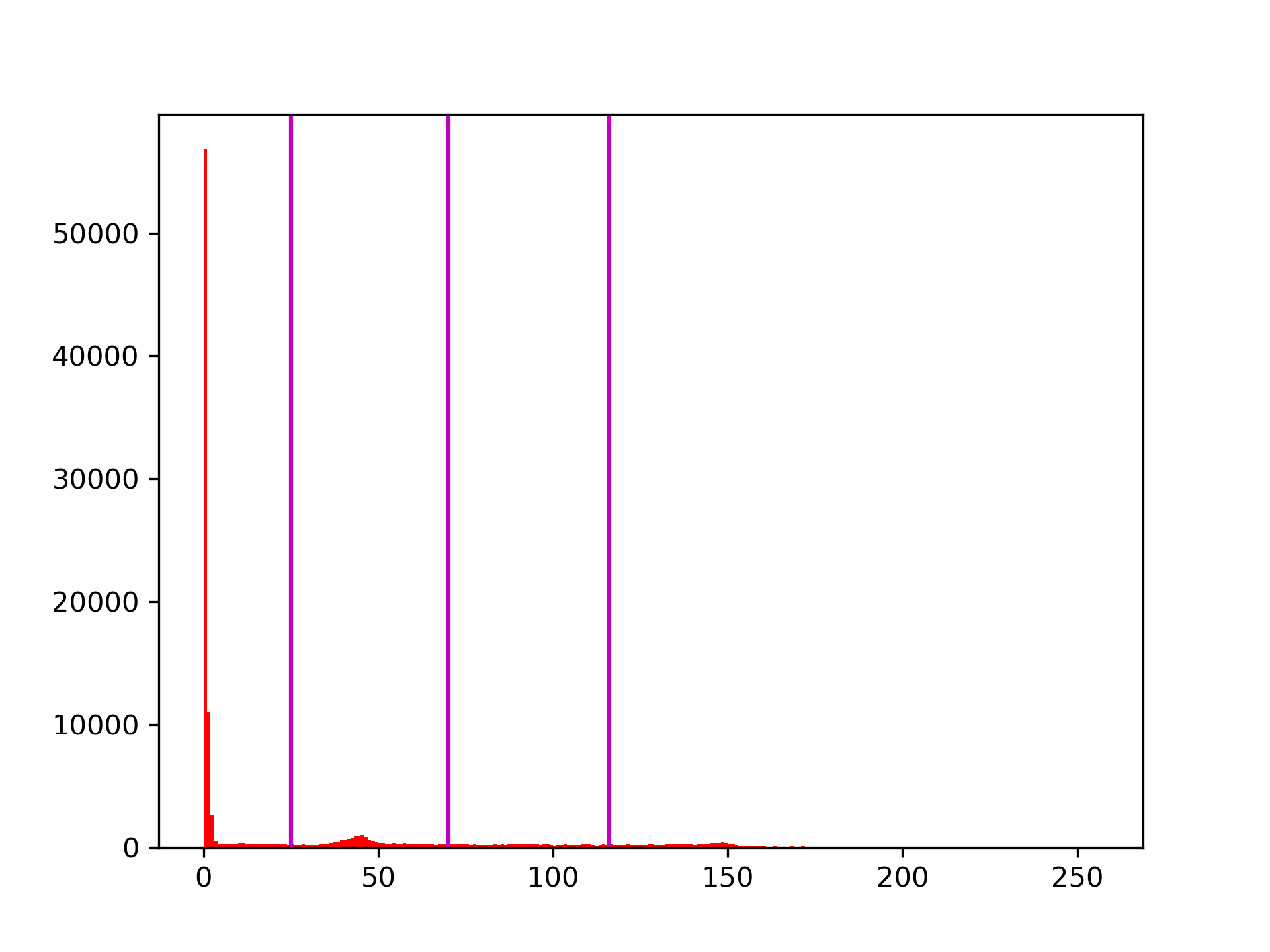
(h) 3 Thresholds

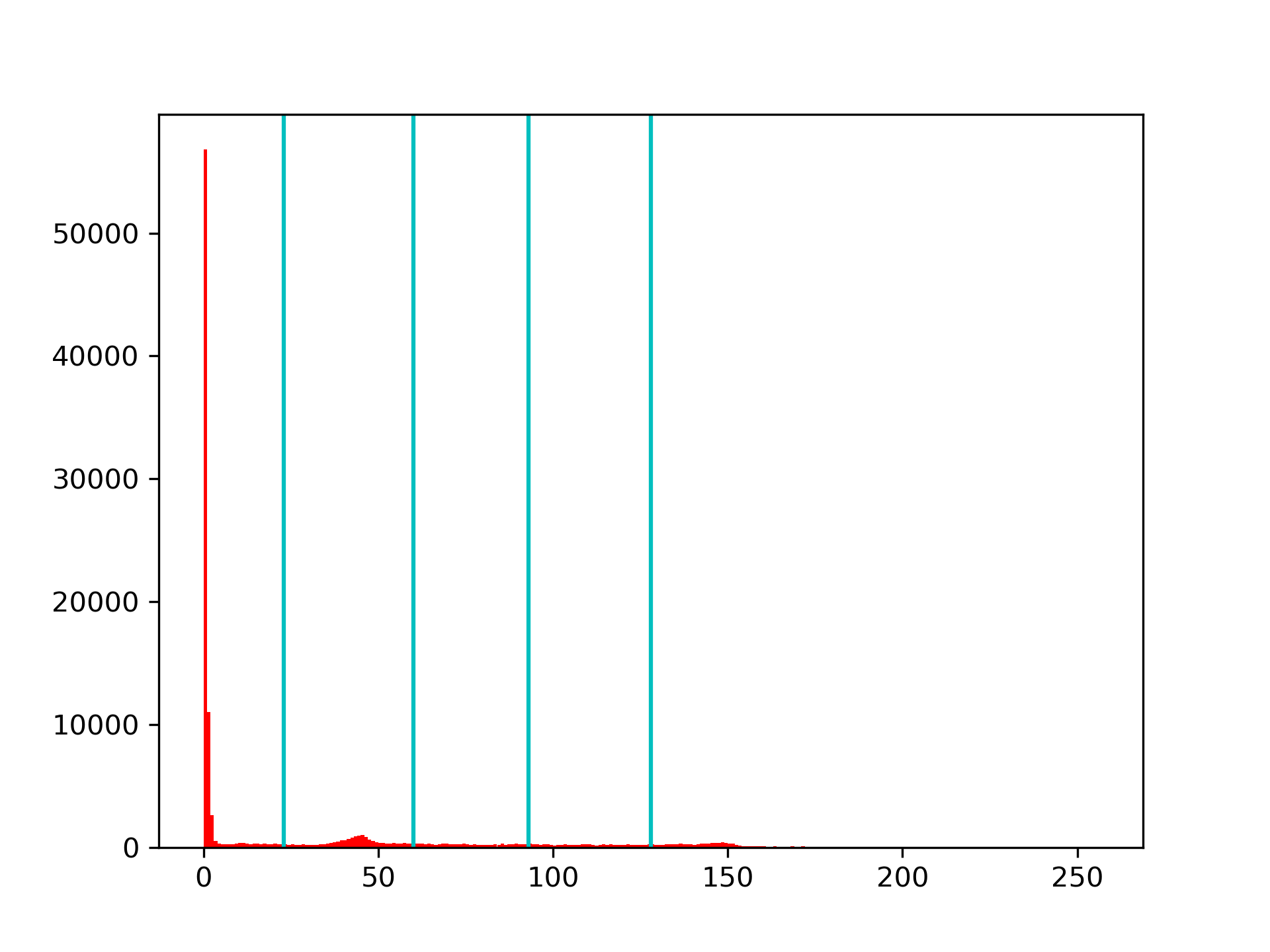
(i) 4 Thresholds

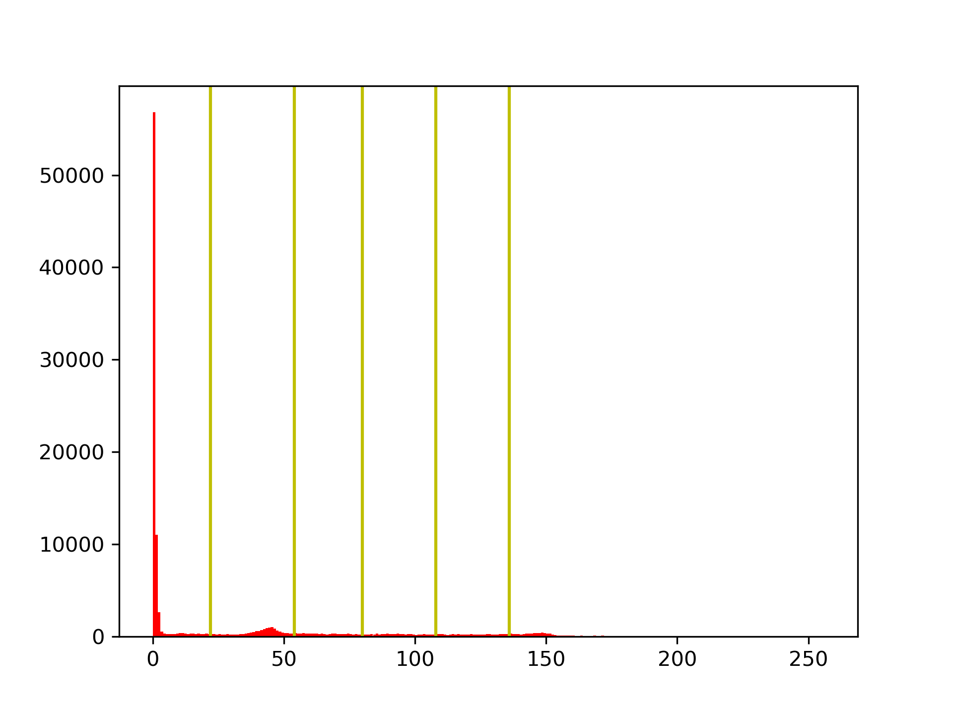
(j) 5 Thresholds

Figure 9: Original image and thresholded images for Brainweb dataset image Z144 with number of thresholds: 2, 3, 4 and 5, with their corresponding histograms and thresholds marked with vertical lines.

Experiments have been performed using 2, 3, 4 and 5 thresholds for the multi-level thresholding problem. Table 1 and Table 2 show the results of the proposed model on the two publicly available datasets used in this study. For each of the images, the high values for the six evaluation metrics justify the fact that the proposed segmentation framework is reliable. The values of the quantitative parameters differ from each other for each of the images and it is also observed that as the number of thresholds is increased for a particular image, the values of the metrics are seen to increase. This is because on increasing the number of thresholds, we get an image that is segmented into more classes and hence, the result. The FSIM, SSIM and PSNR metrics are generally used to gauge the quality of the segmented image by drawing a comparison with the original image. HPSI measures the visual similarity between two images with respect to a human observer. UIQI is used in comparison by modelling the image distortion which comprises loss of correlation, luminance and contrast. QILV is used to measure the non-stationarity of an image by centring on the basic image structure. Figures 2, 3, 4 and 5 show some qualitative results from the experiments on the Harvard WBA dataset and Figures 6, 7, 8 and 9 show some qualitative results from the Brainweb dataset using number of thresholds as 2, 3, 4 and 5 respectively. In each of the figures, we have placed the initial image, as well as the thresholded images by varying the number of thresholds. We have also included a graph marking the point of each of the thresholds for each of our thresholded images.

Table 3: Quantitative results as obtained on using various chaotic maps while initializing the feature vectors in HHO

Chaotic map	No. of Thresholds	PSNR	SSIM	FSIM	UIQI	QILV	HPSI
No map	2	23.0206	0.8162	0.7949	0.4371	0.7426	0.6863
	3	24.9477	0.8658	0.8603	0.5442	0.8440	0.7867
	4	26.4417	0.8960	0.8961	0.6215	0.8935	0.8389
	5	27.5454	0.9158	0.9205	0.6779	0.9223	0.8711
Sine	2	23.0206	0.8194	0.7959	0.4396	0.7426	0.6893
	3	24.8599	0.8681	0.8619	0.5478	0.8396	0.7900
	4	26.5405	0.8983	0.8983	0.6250	0.8947	0.8423
	5	27.5543	0.9146	0.9220	0.6744	0.9213	0.8746
Singer	2	23.0206	0.8162	0.7949	0.4371	0.7426	0.6852
	3	24.9173	0.8658	0.8603	0.5442	0.8418	0.7867
	4	26.3635	0.8972	0.8992	0.6242	0.8921	0.8440
	5	27.6836	0.9159	0.9211	0.6777	0.9237	0.8737
Sinusoidal	2	22.8736	0.8167	0.7945	0.4366	0.7381	0.6863
	3	24.9147	0.8657	0.8584	0.5419	0.8434	0.7813
	4	26.3635	0.8988	0.8992	0.6277	0.8898	0.8440
	5	27.6072	0.9192	0.9226	0.6844	0.9216	0.8766
Chebyshev	2	23.0206	0.8162	0.7949	0.4371	0.7426	0.6863
	3	24.9477	0.8636	0.8599	0.5395	0.8440	0.7875
	4	26.4528	0.8978	0.8980	0.6241	0.8925	0.8422
	5	27.6964	0.9175	0.9235	0.6805	0.9227	0.8785
Tent	2	22.9281	0.8174	0.7956	0.4382	0.7412	0.6904
	3	24.9173	0.8658	0.8603	0.5442	0.8418	0.7867
	4	26.4464	0.8997	0.8975	0.6280	0.8942	0.8413
	5	27.6484	0.9175	0.9235	0.6803	0.9216	0.8785
Logistic	2	23.0206	0.8174	0.7949	0.4382	0.7426	0.6852
	3	24.8212	0.8651	0.8602	0.5426	0.8408	0.7843
	4	26.3912	0.8972	0.8992	0.6242	0.8936	0.8440
	5	27.7382	0.9197	0.9230	0.6852	0.9239	0.8764
Iterative	2	22.9959	0.8202	0.7959	0.4415	0.7415	0.6893
	3	24.9477	0.8663	0.8615	0.5446	0.8440	0.7924
	4	26.3417	0.8966	0.8993	0.6238	0.8935	0.8443
	5	27.6072	0.9192	0.9226	0.6844	0.9218	0.8766
Gauss	2	22.9585	0.8137	0.7945	0.4343	0.7424	0.6863
	3	25.0224	0.8667	0.8600	0.5443	0.8445	0.7886
	4	26.2731	0.8939	0.8969	0.6181	0.8882	0.8396
	5	27.5186	0.9159	0.9208	0.6777	0.9217	0.8743

Table 3 thus demonstrates that amongst the various maps given, the one that gives the best results is the Logistic map. The values are provided in the table for each of the maps, for each threshold, and are computed by averaging each of the evaluation parameters, for all the images used in this paper. As expected, the chaotic maps boost the performance by increasing the diversity of the solutions. It is seen that the metrics obtained for most of the maps are very close to each other and differ marginally. Since the performance delivered by the Logistic chaotic map is the best, we use this particular map while doing further experiments.

Table 4: Comparison in performance of the proposed framework based on the objective function for fitness assignment to the Harris hawks population.

Objective Function	No. of thresholds	PSNR	SSIM	FSIM	UIQI	QILV	HPSI
Cross Entropy	2	18.8024	0.7158	0.7553	0.2720	0.6109	0.5665
	3	20.4756	0.7703	0.8151	0.3389	0.7542	0.7001
	4	22.2979	0.8242	0.8577	0.4099	0.8139	0.7705
	5	23.6517	0.8555	0.8866	0.4676	0.8545	0.8167
Mean Squared Error	2	17.0006	0.5524	0.6512	0.2234	0.7231	0.3524
	3	18.3757	0.6121	0.7019	0.2903	0.7999	0.4120
	4	19.6511	0.6574	0.7420	0.3509	0.8653	0.4622
	5	20.8165	0.6976	0.7764	0.4031	0.9059	0.5076
Proposed Objective Function	2	18.6361	0.7077	0.7621	0.2709	0.7008	0.5810
	3	20.5767	0.7823	0.8162	0.3451	0.8215	0.7136
	4	23.5121	0.8132	0.8740	0.4212	0.8456	0.7816
	5	24.7360	0.8410	0.8842	0.4531	0.9093	0.8142
Proposed Hybrid	2	19.6240	0.7176	0.7652	0.2711	0.7098	0.5818
	3	21.8767	0.7913	0.8368	0.3549	0.8258	0.7285
	4	23.5343	0.8251	0.8741	0.4237	0.8725	0.7857
	5	24.7686	0.8608	0.8959	0.4670	0.9192	0.8228

Table 4 outlines the quantitative results obtained by different objective functions used for fitness assignment in the HHO algorithm. Evidently, the proposed hybrid objective function performs better than the rest, where the weights are set as: $\alpha=0.35$ and $\beta=0.65$ experimentally. The hybrid objective function augments the values of all the metrics, as is evident from the results. There is a clear gap between the values returned by this function and those returned by the other objective functions.

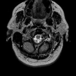
(a) Original

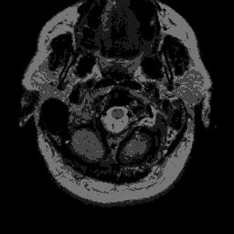
(b) 2 Thresholds

(c) 3 Thresholds

(d) 4 Thresholds

(e) 5 Thresholds

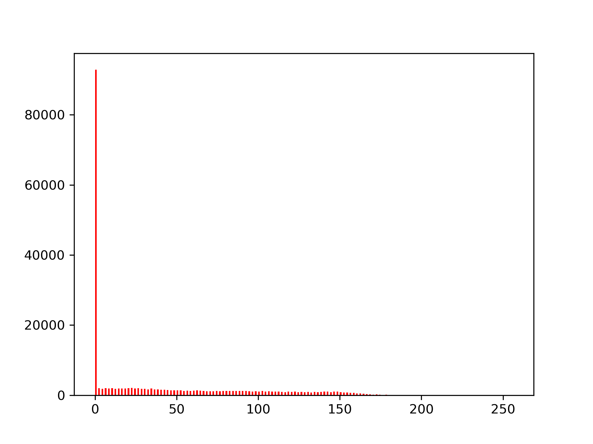
(f) Original

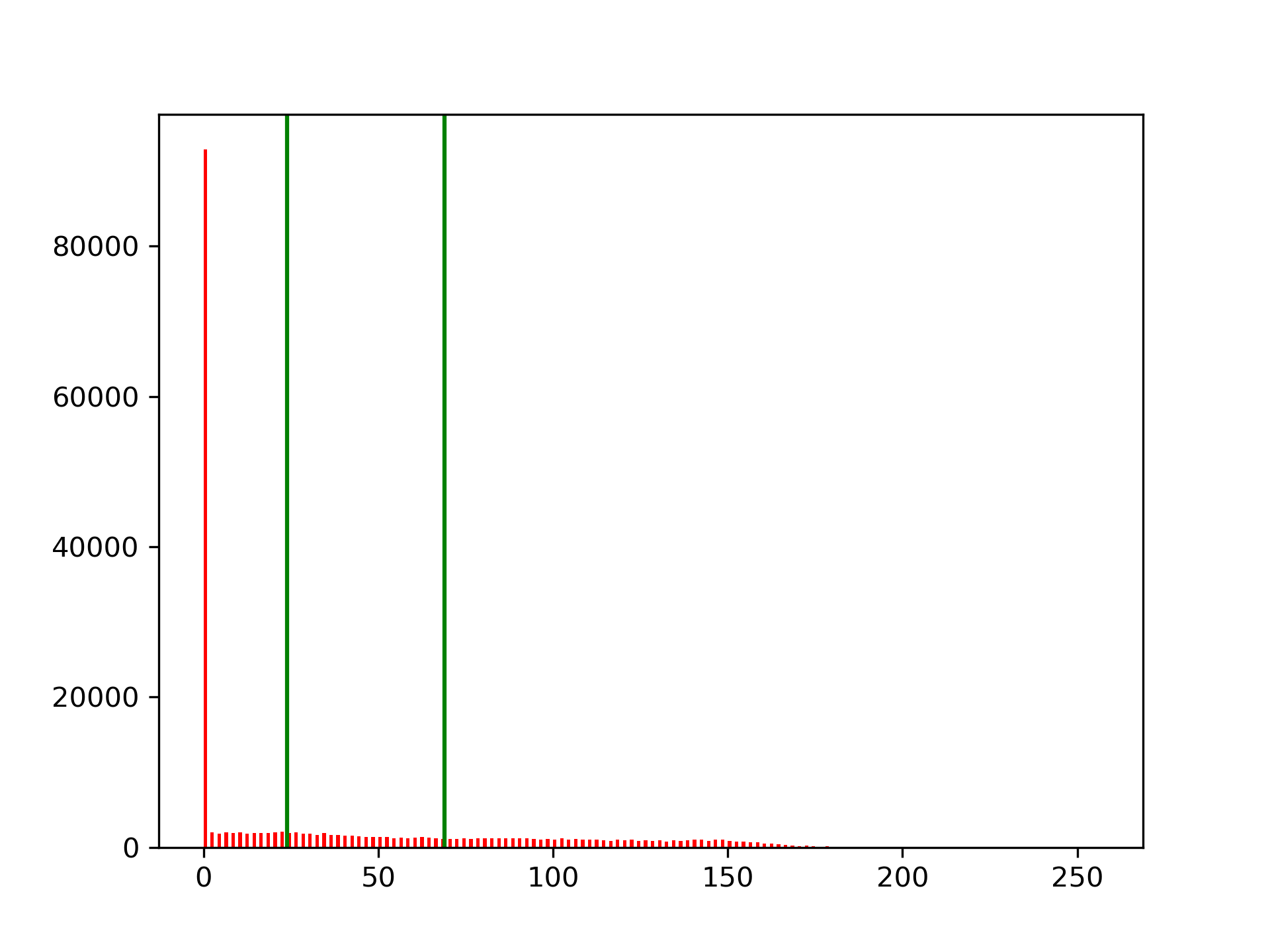
(g) 2 Thresholds

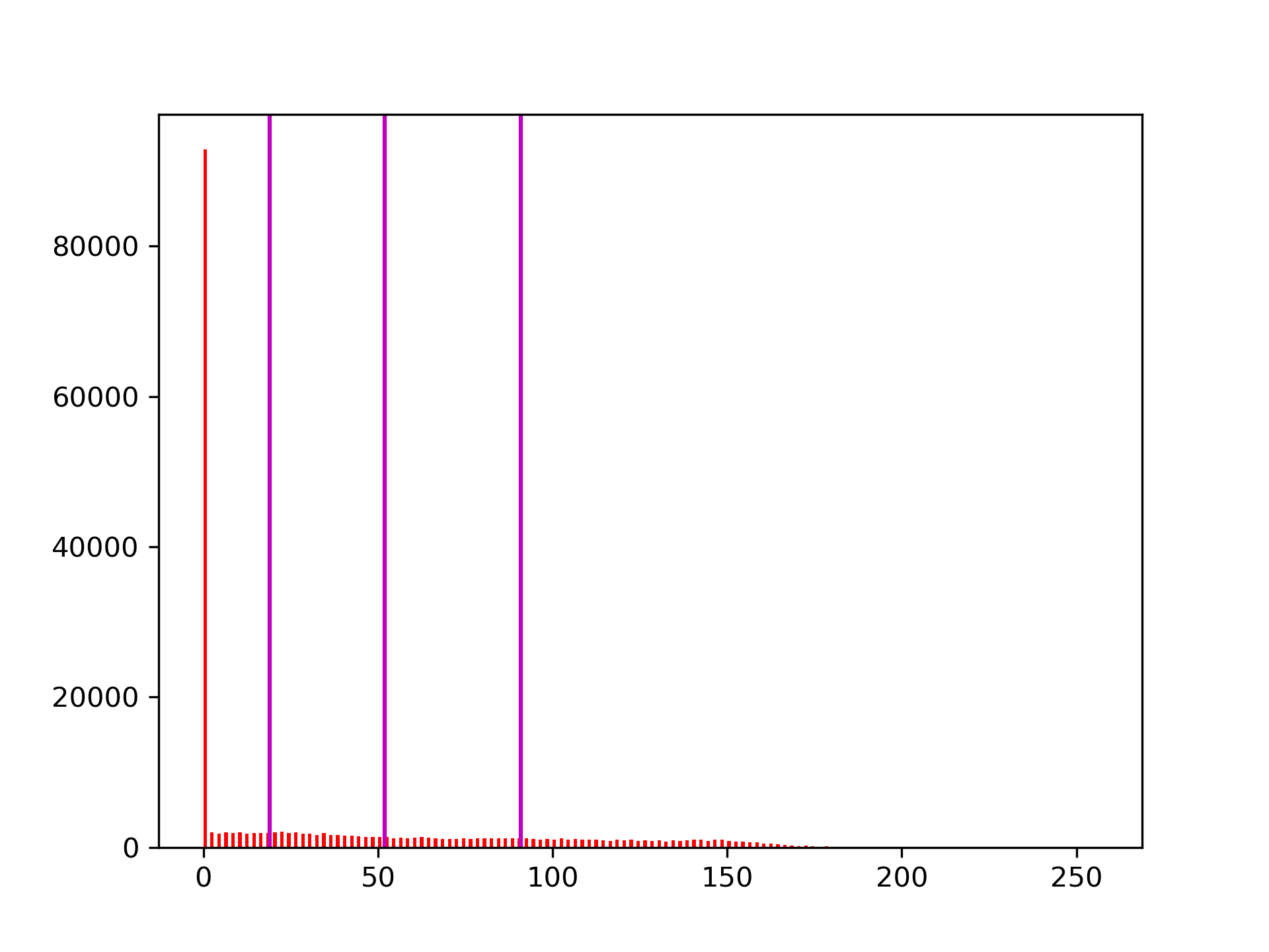
(h) 3 Thresholds

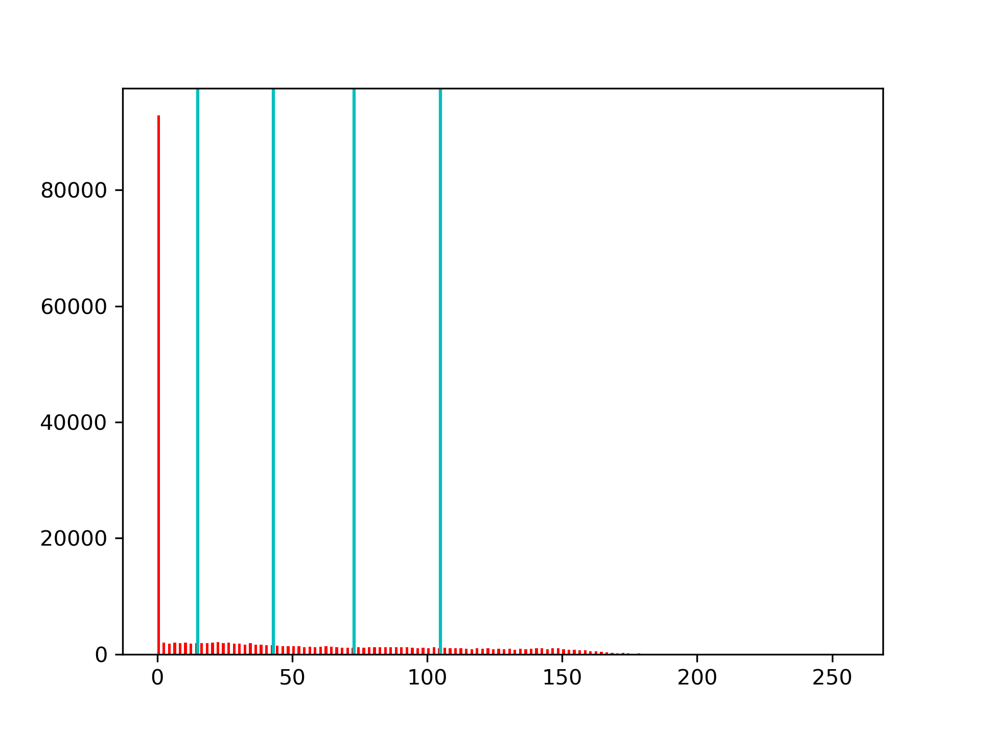
(i) 4 Thresholds

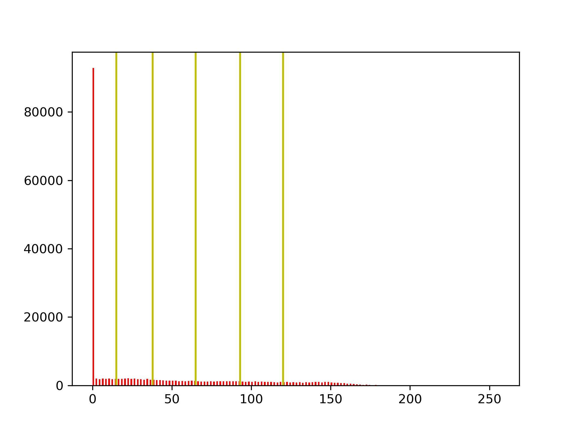
(j) 5 Thresholds

Figure 2: Original image and thresholded images for slice 22 of the Harvard WBA dataset with number of thresholds: 2, 3, 4 and 5, with their corresponding histograms and thresholds marked with vertical lines.

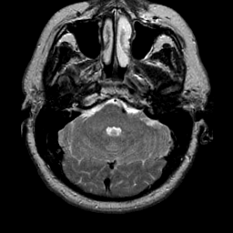
(a) Original

(b) 2 Thresholds

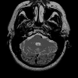
(c) 3 Thresholds

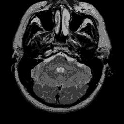
(d) 4 Thresholds

(e) 5 Thresholds

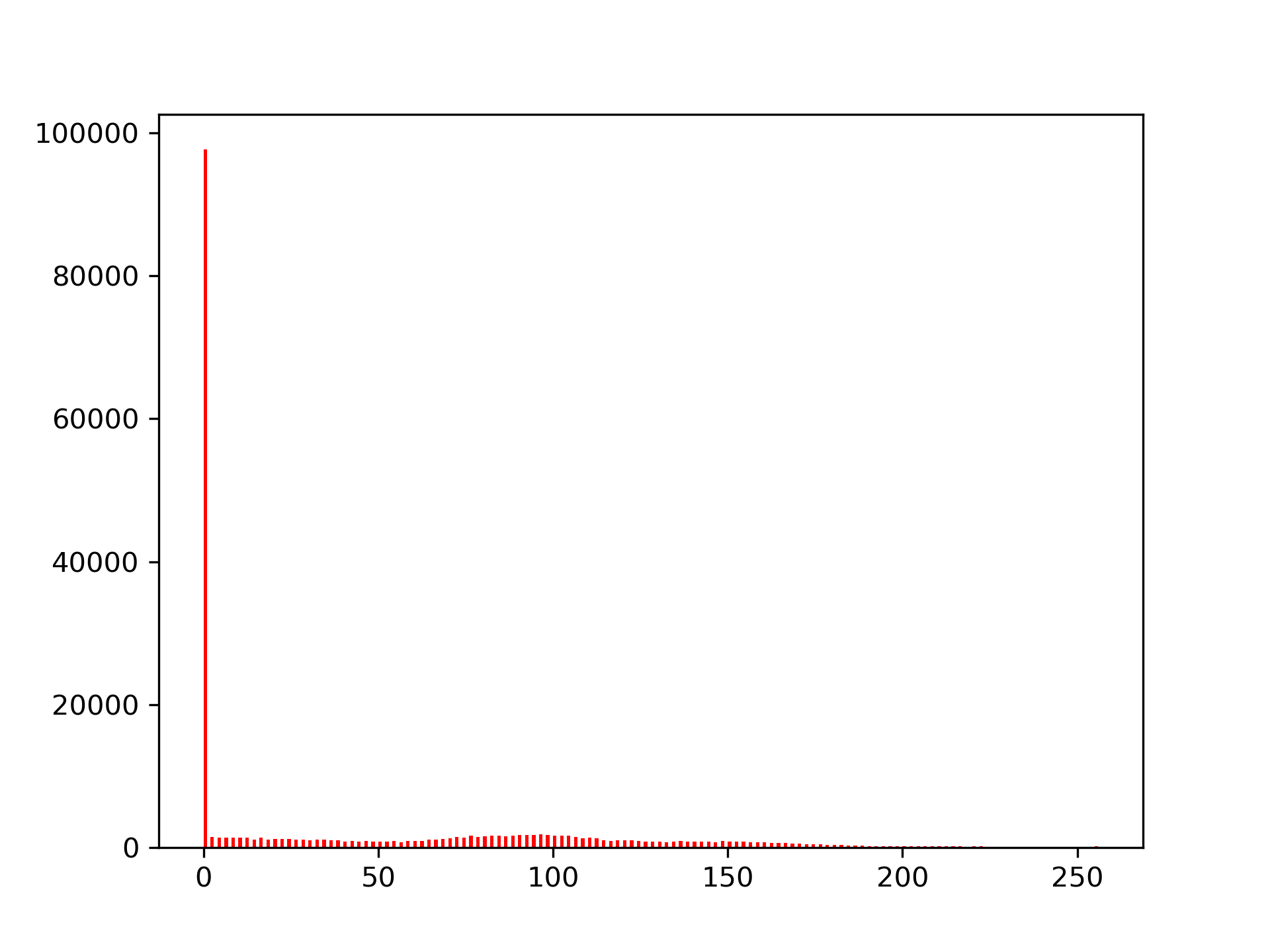
(f) Original

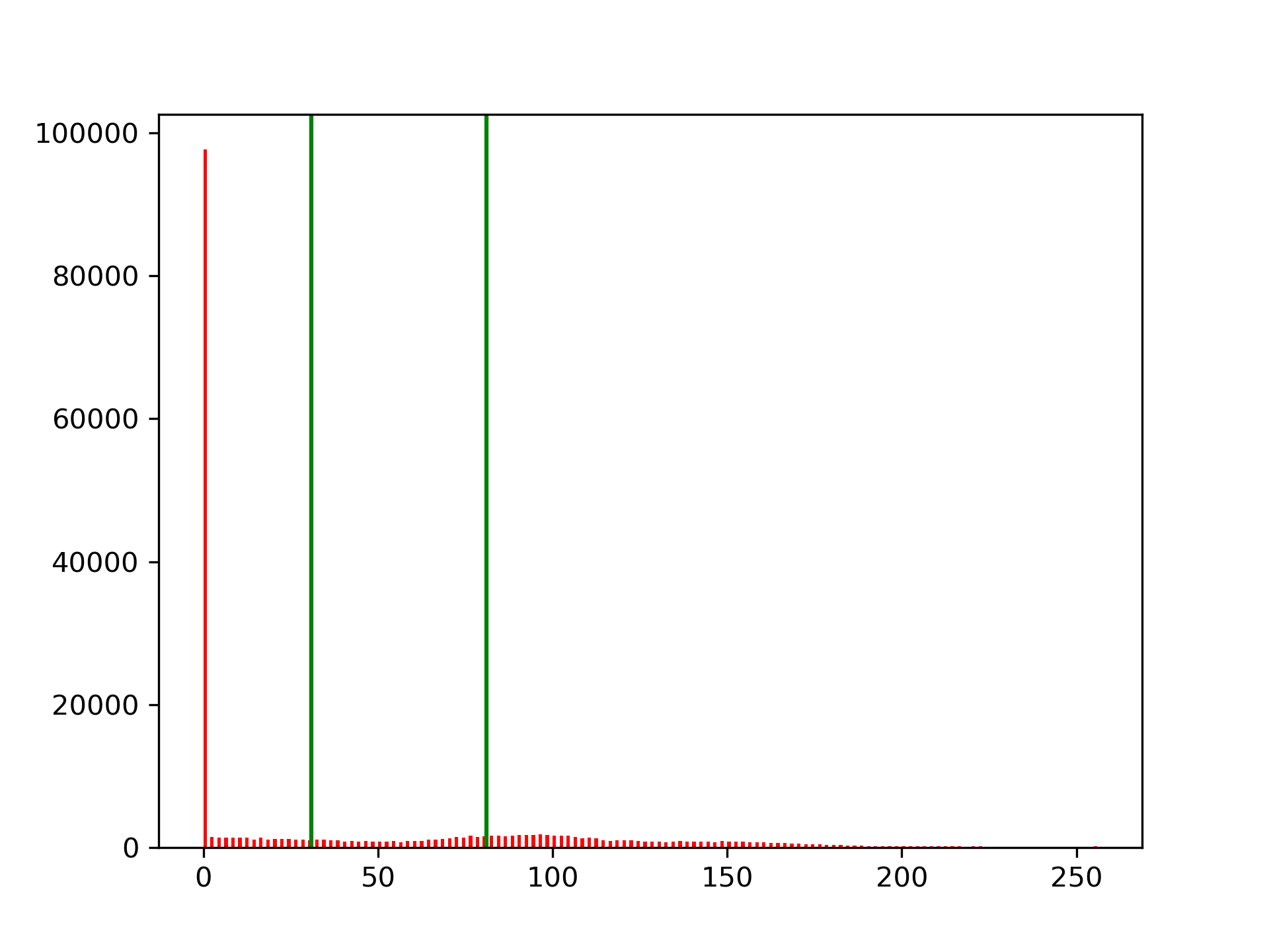
(g) 2 Thresholds

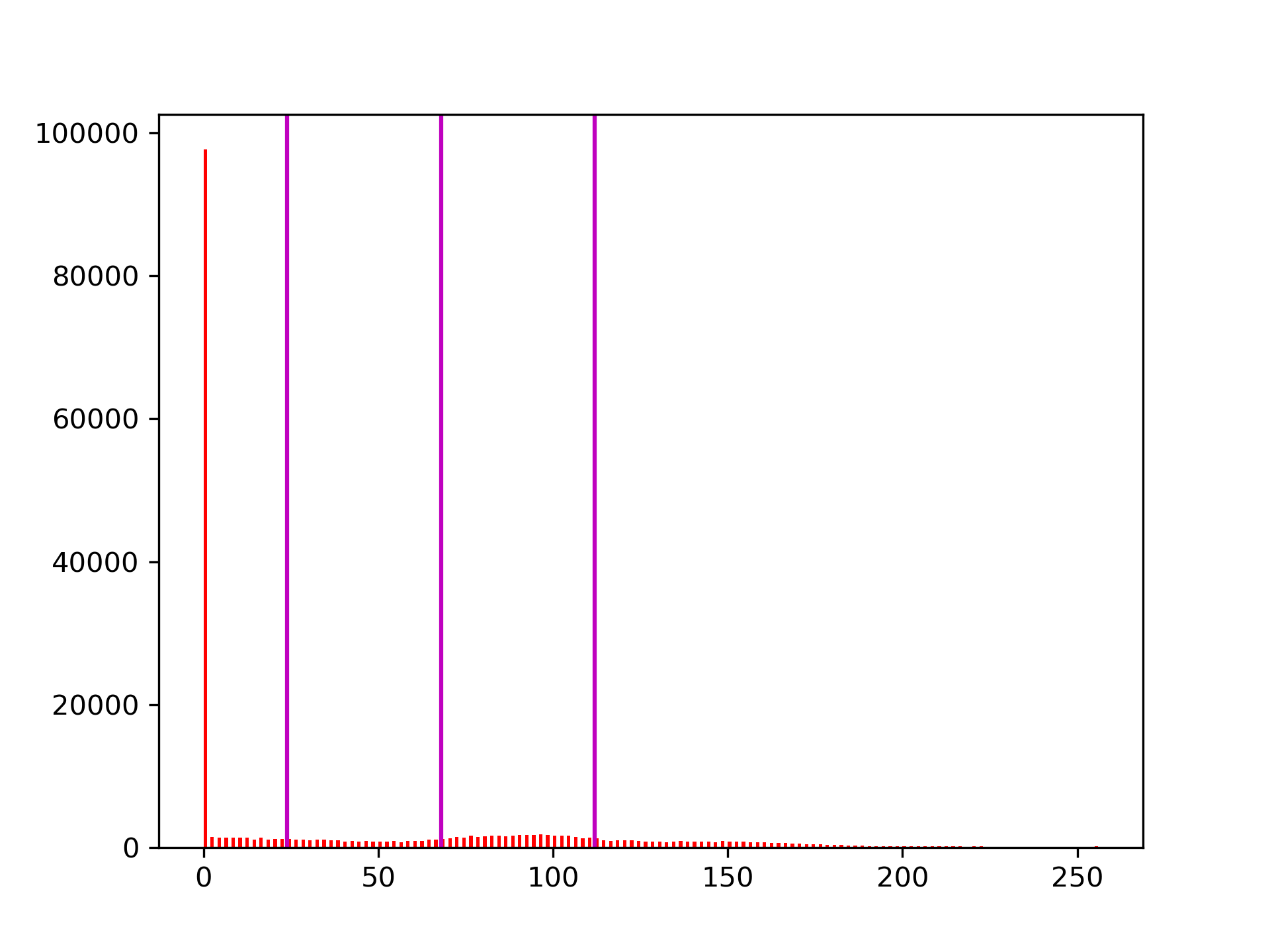
(h) 3 Thresholds

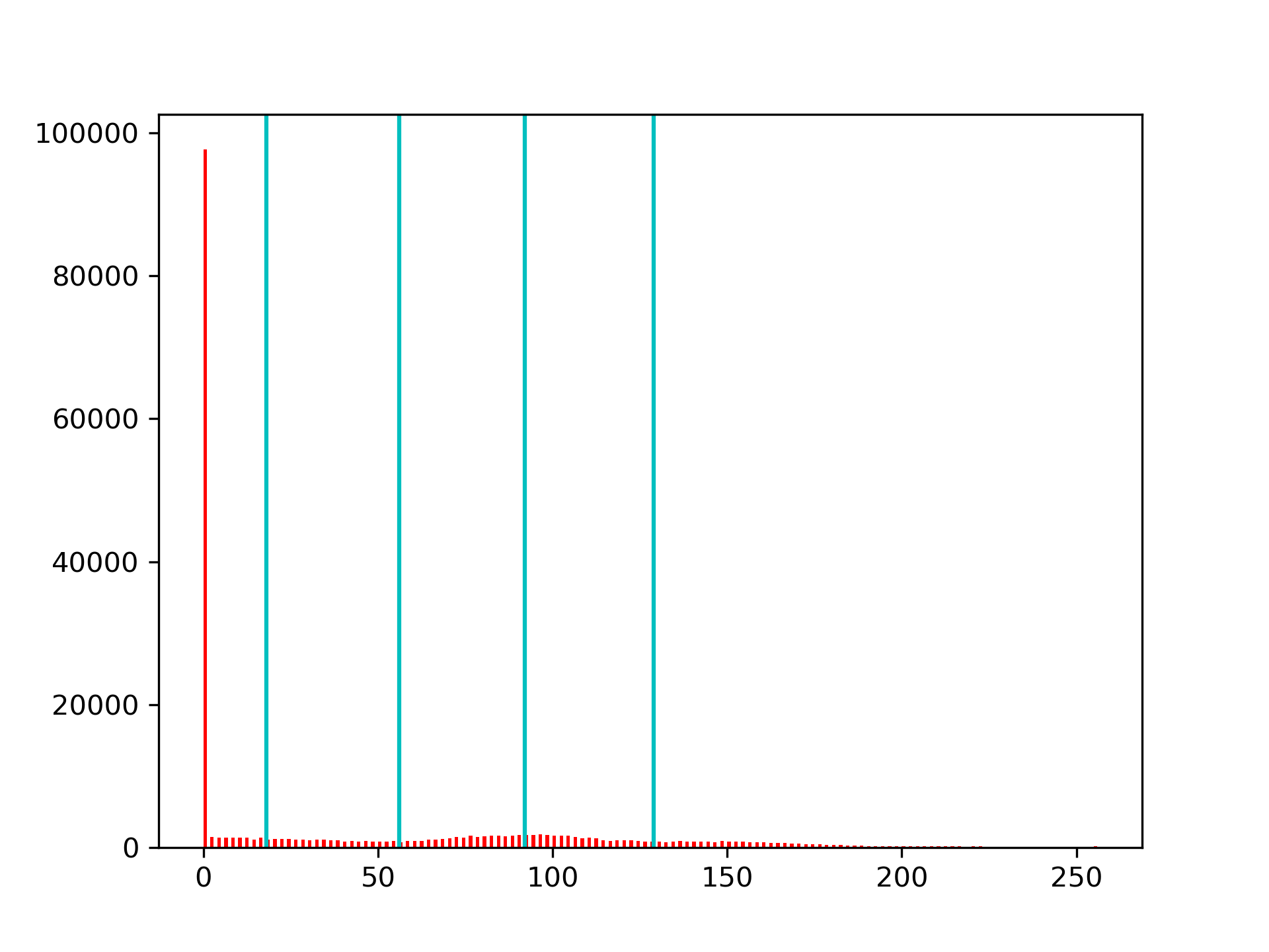
(i) 4 Thresholds

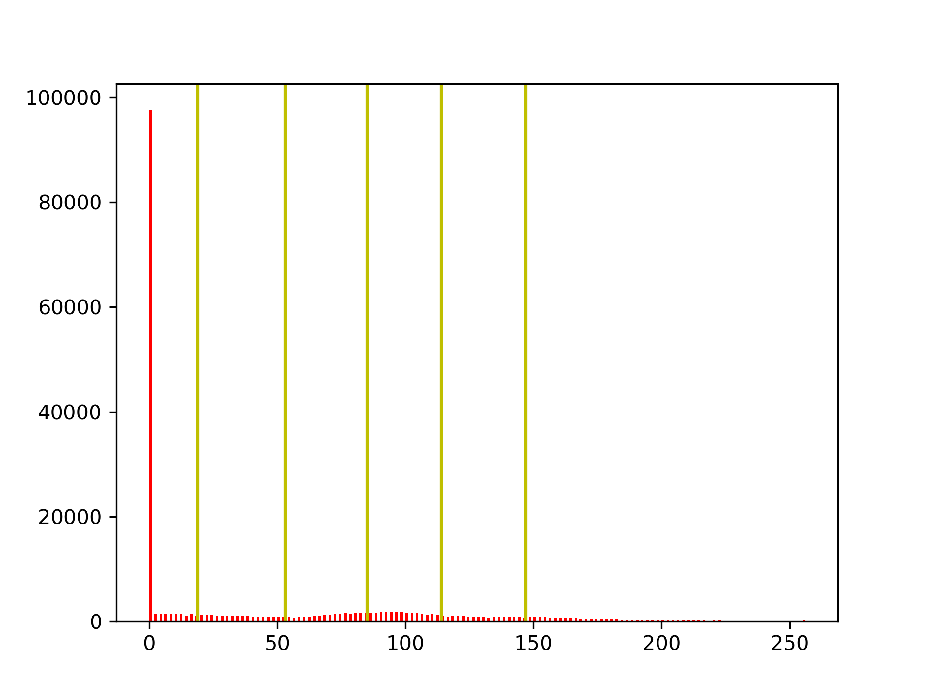
(j) 5 Thresholds

Figure 3: Original image and thresholded images for slice 42 of the Harvard WBA dataset with number of thresholds: 2, 3, 4 and 5, with their corresponding histograms and thresholds marked with vertical lines.

(a) Original

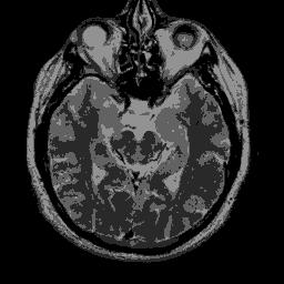
(b) 2 Thresholds

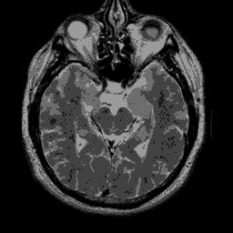
(c) 3 Thresholds

(d) 4 Thresholds

(e) 5 Thresholds

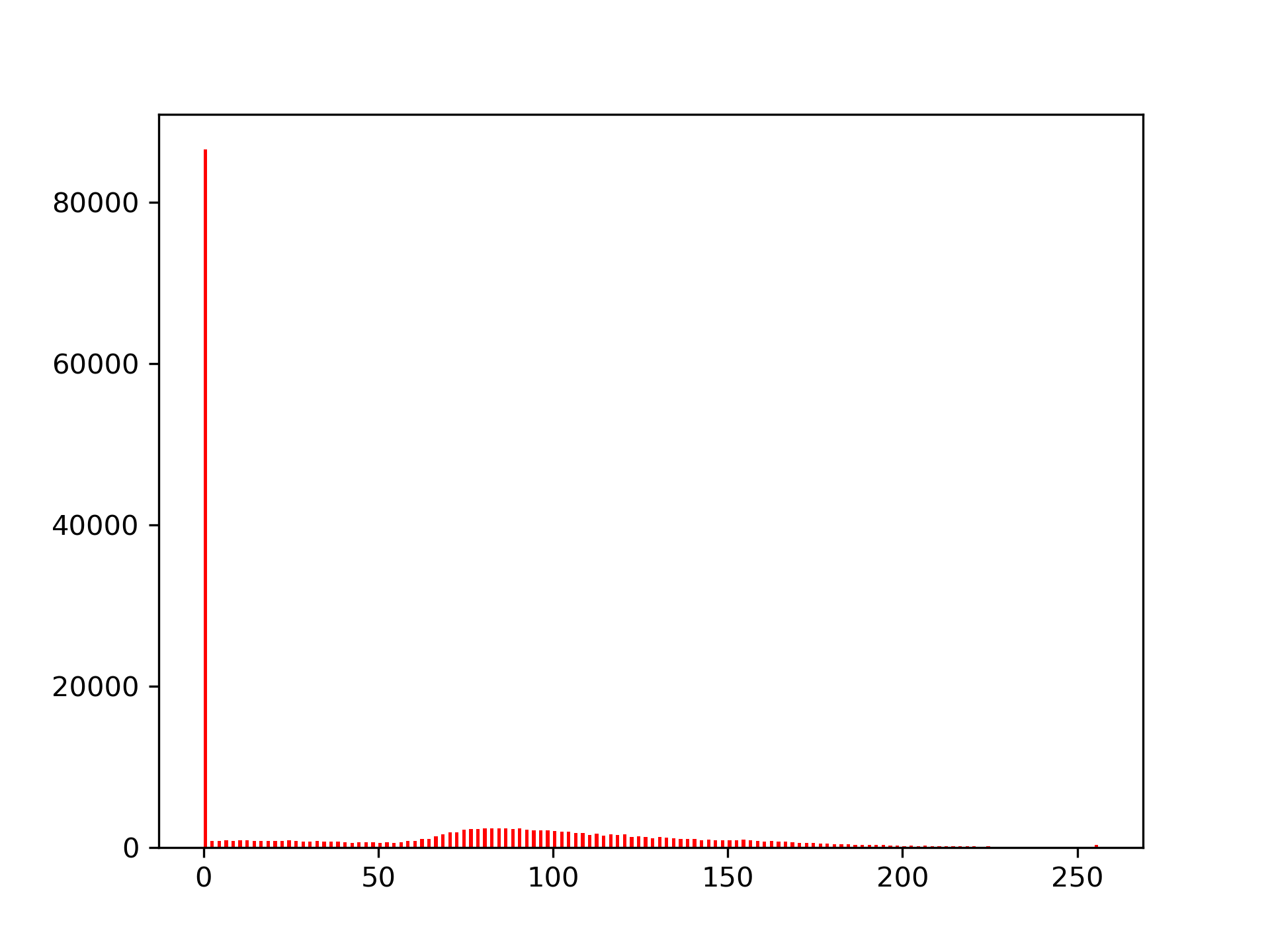
(f) Original

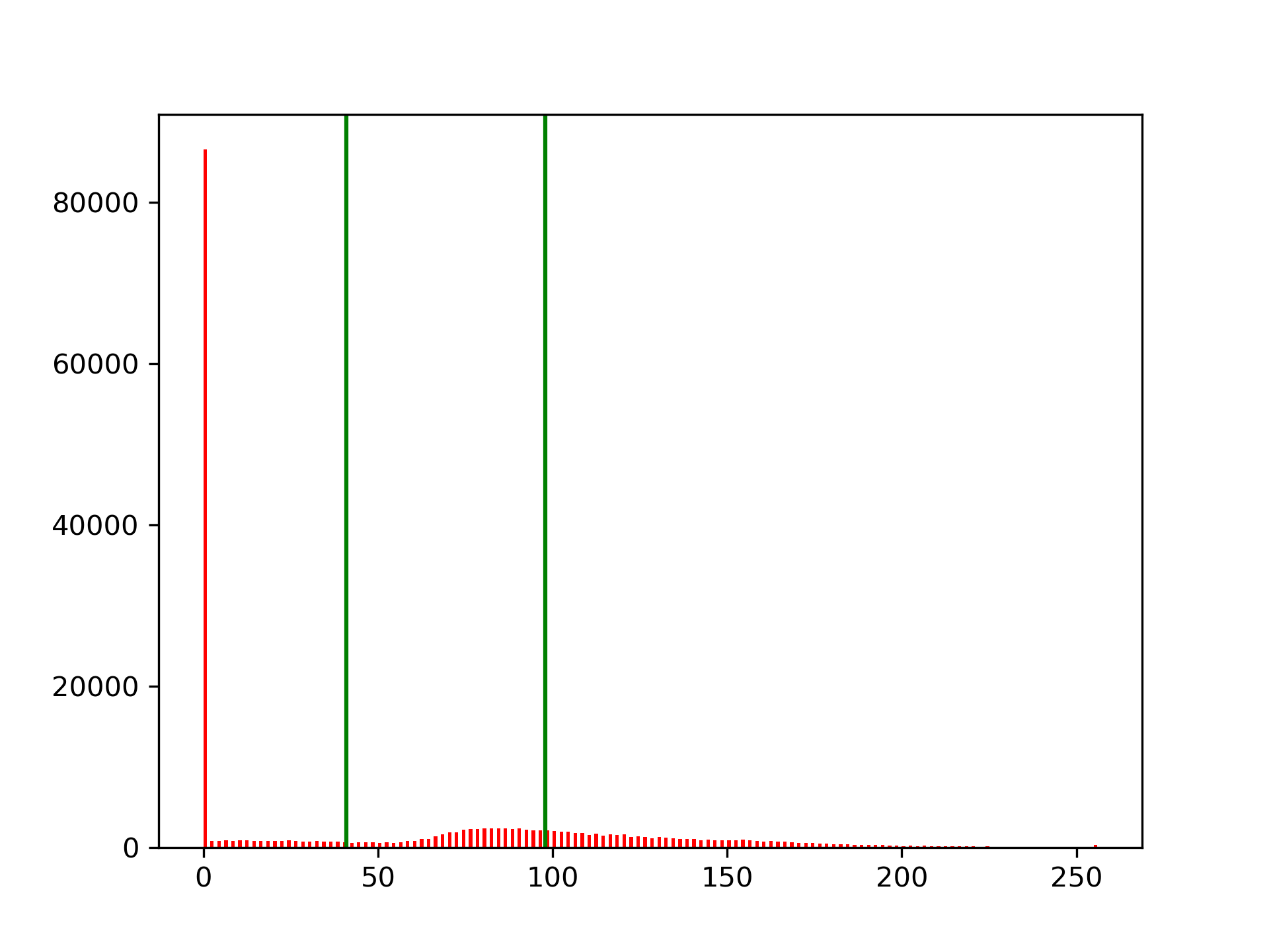
(g) 2 Thresholds

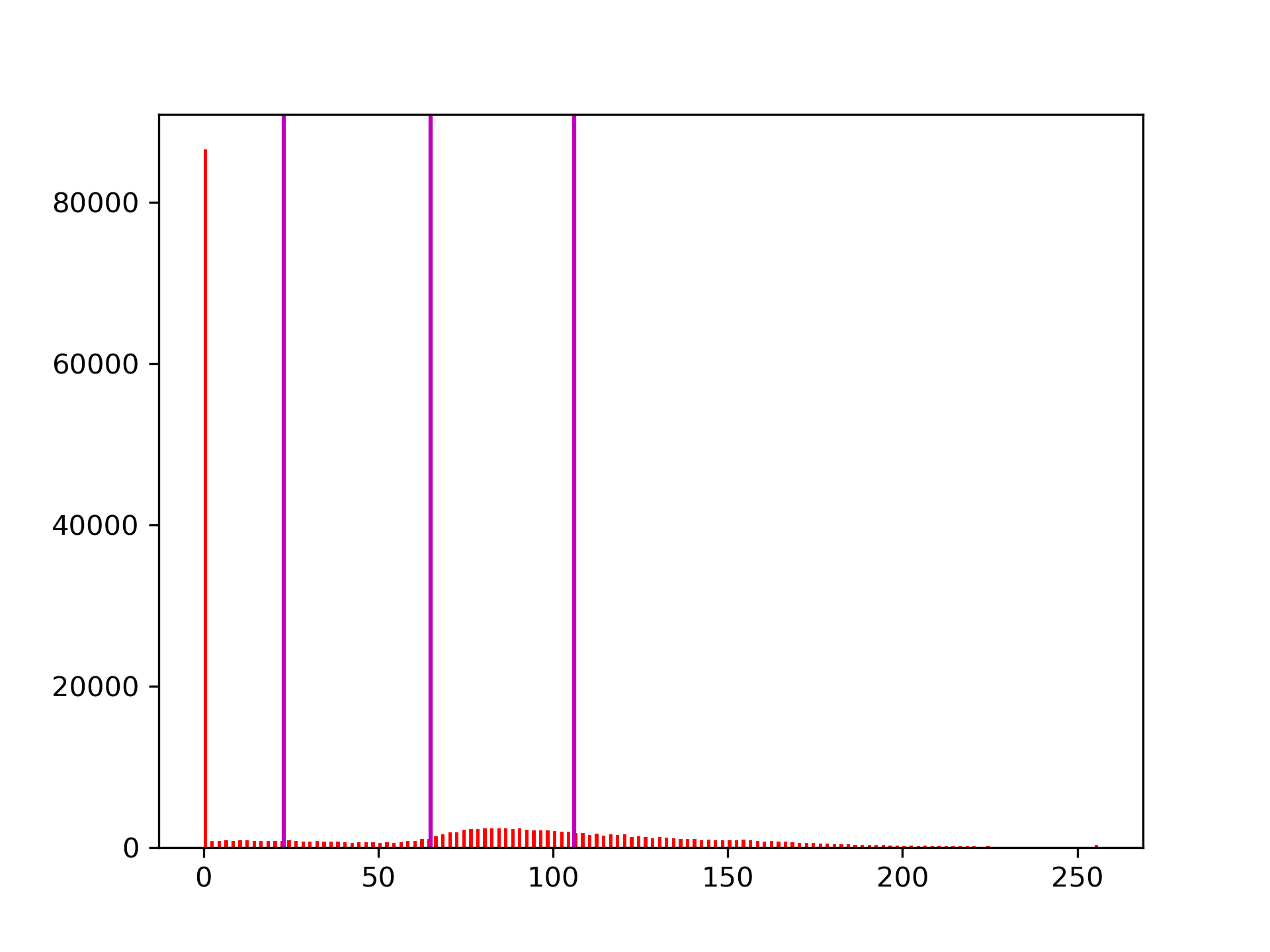
(h) 3 Thresholds

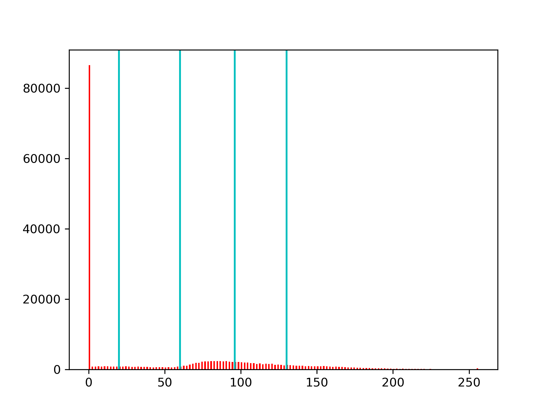
(i) 4 Thresholds

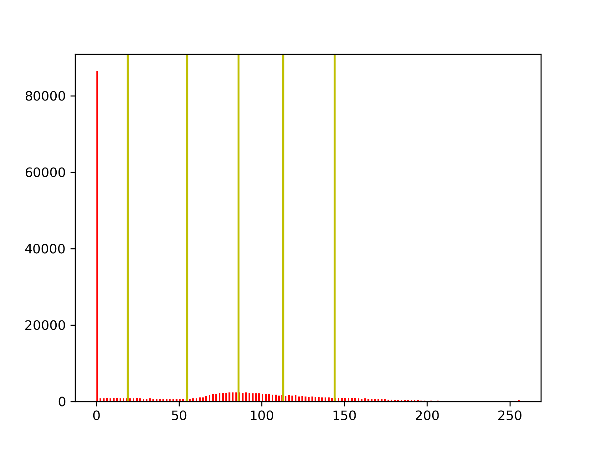
(j) 5 Thresholds

Figure 4: Original image and thresholded images for slice 62 of the Harvard WBA dataset with number of thresholds: 2, 3, 4 and 5, with their corresponding histograms and thresholds marked with vertical lines.

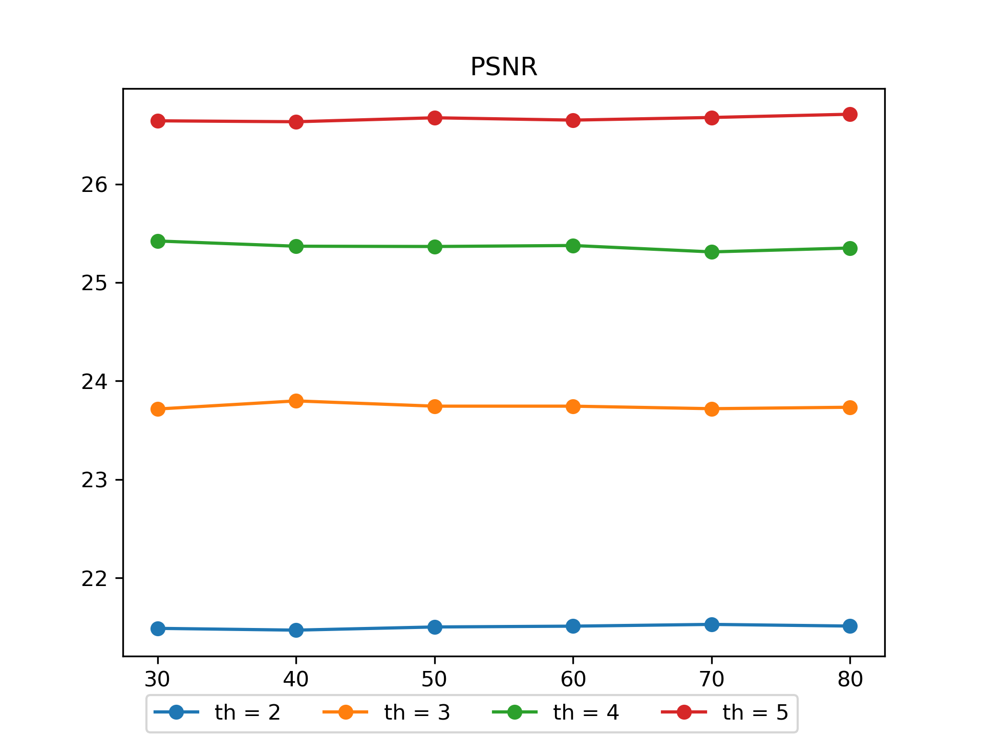
(a) Harvard PSNR

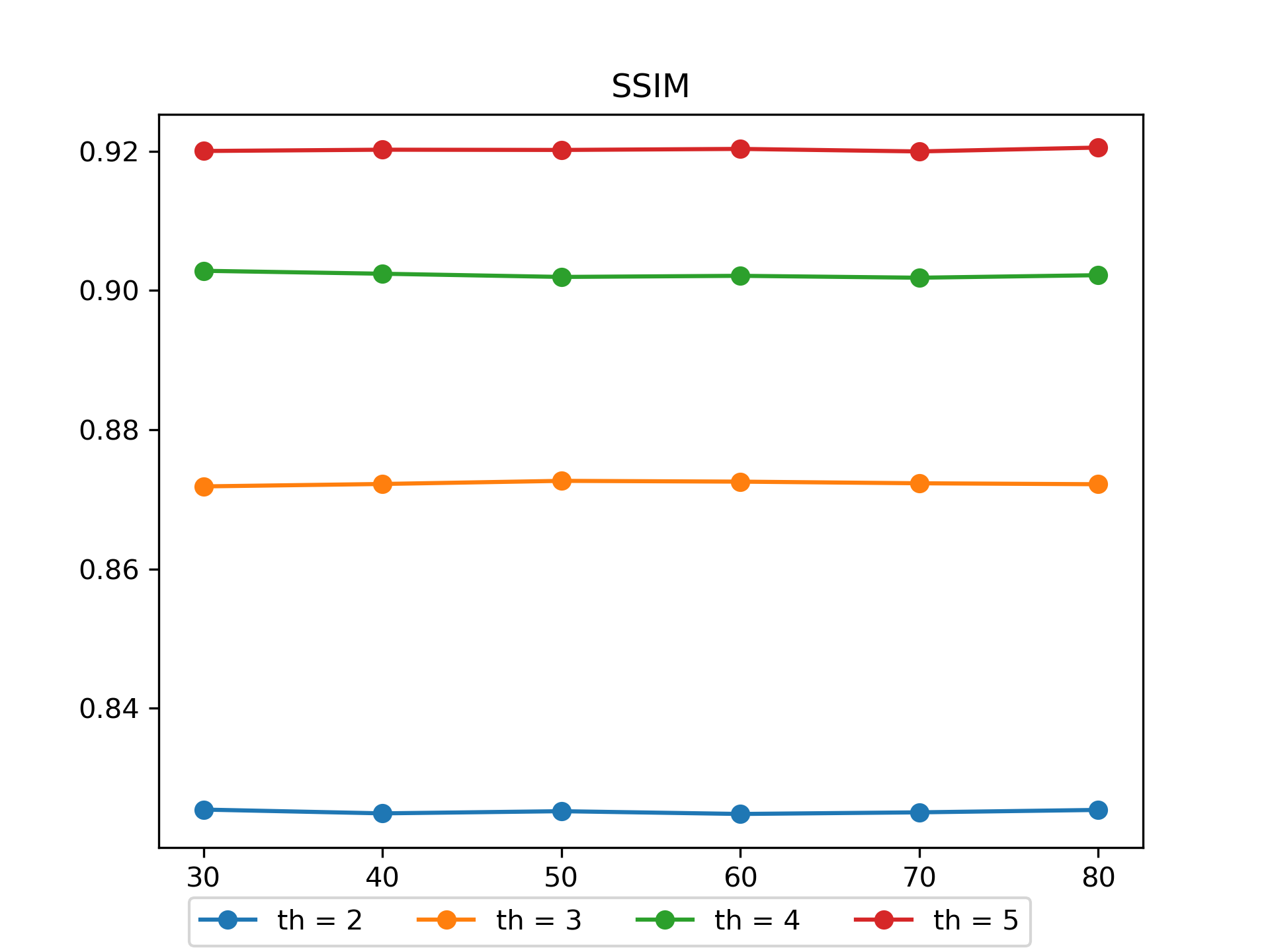
(b) Harvard SSIM

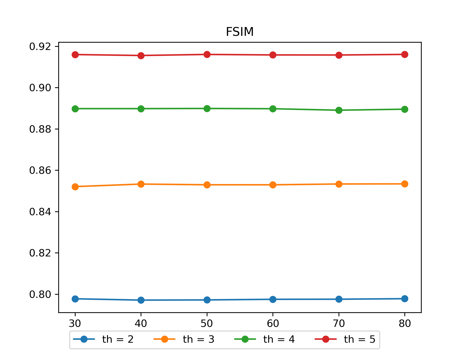
(c) Harvard FSIM

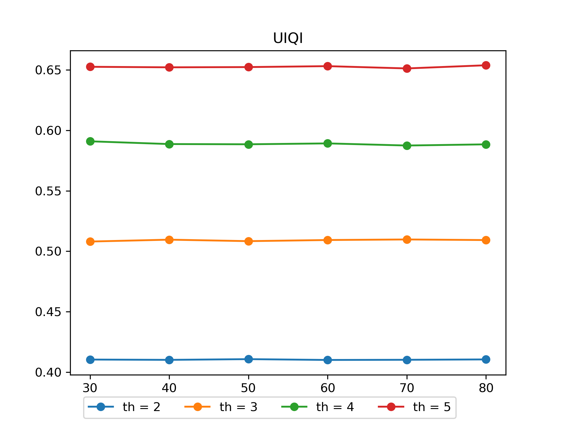
(d) Harvard UIQI

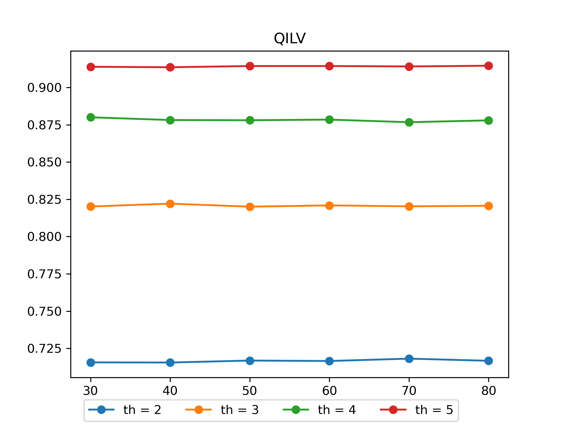
(e) Harvard QILV

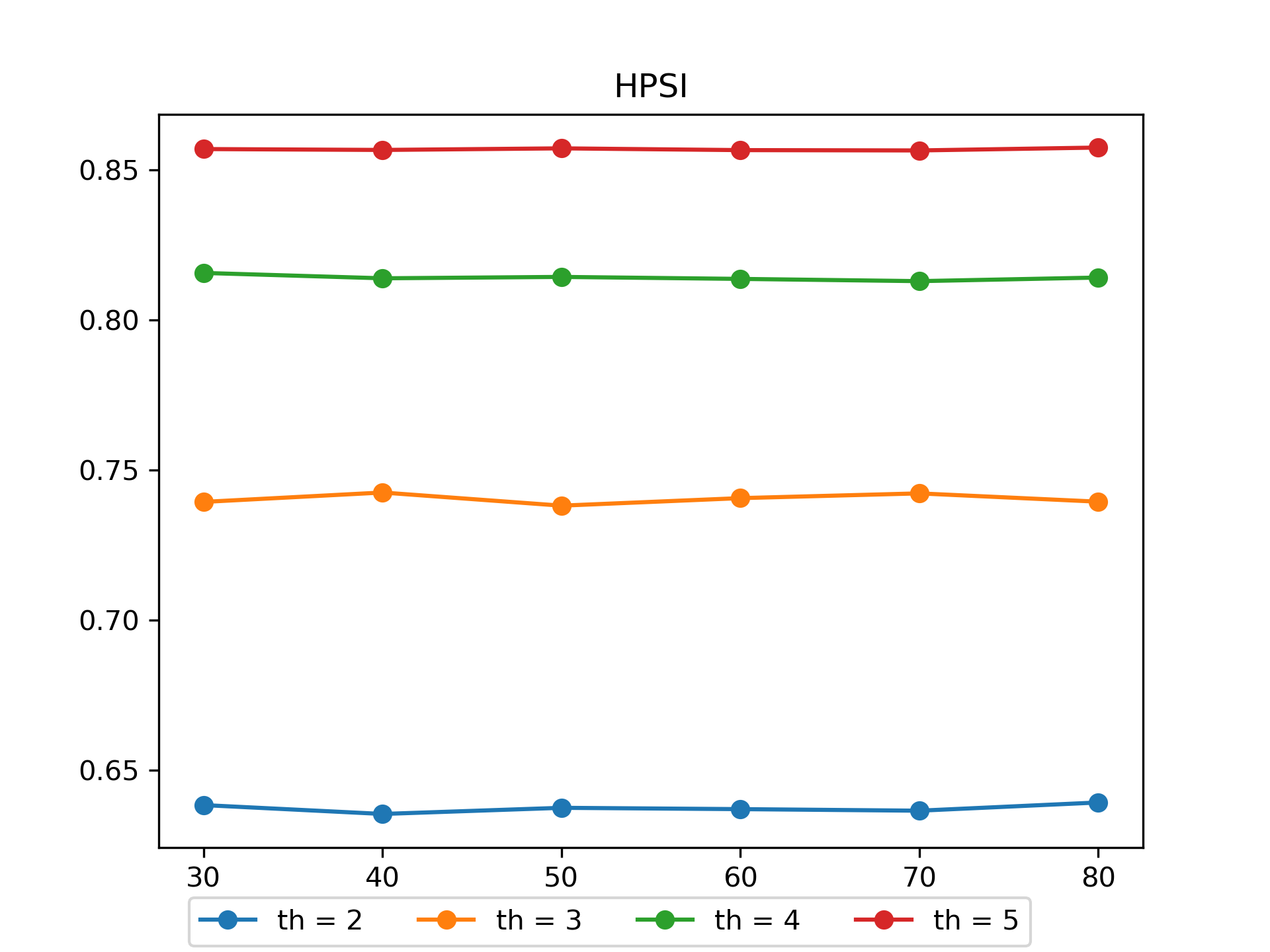
(f) Harvard HPSI

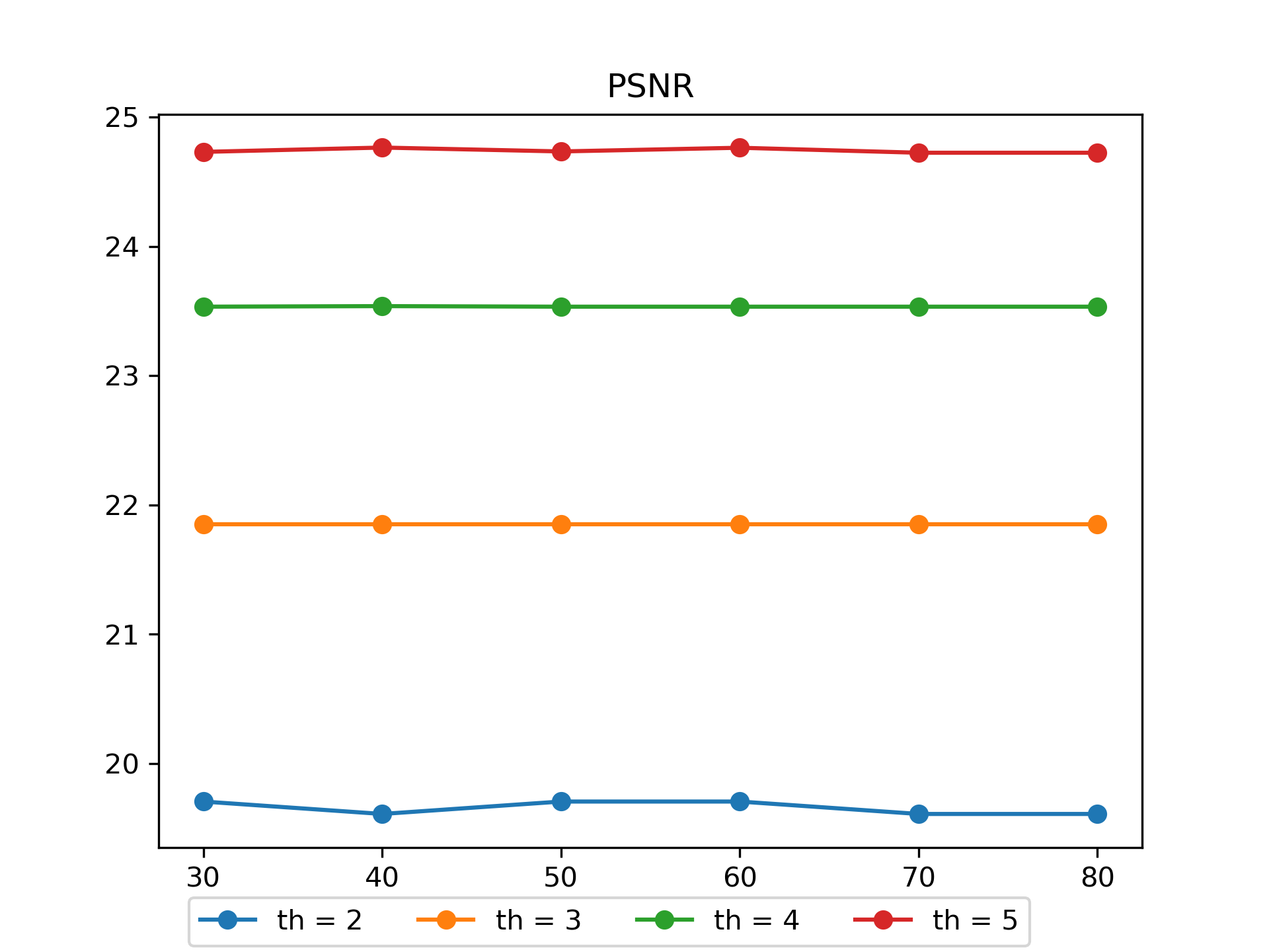
(g) Brainweb PSNR

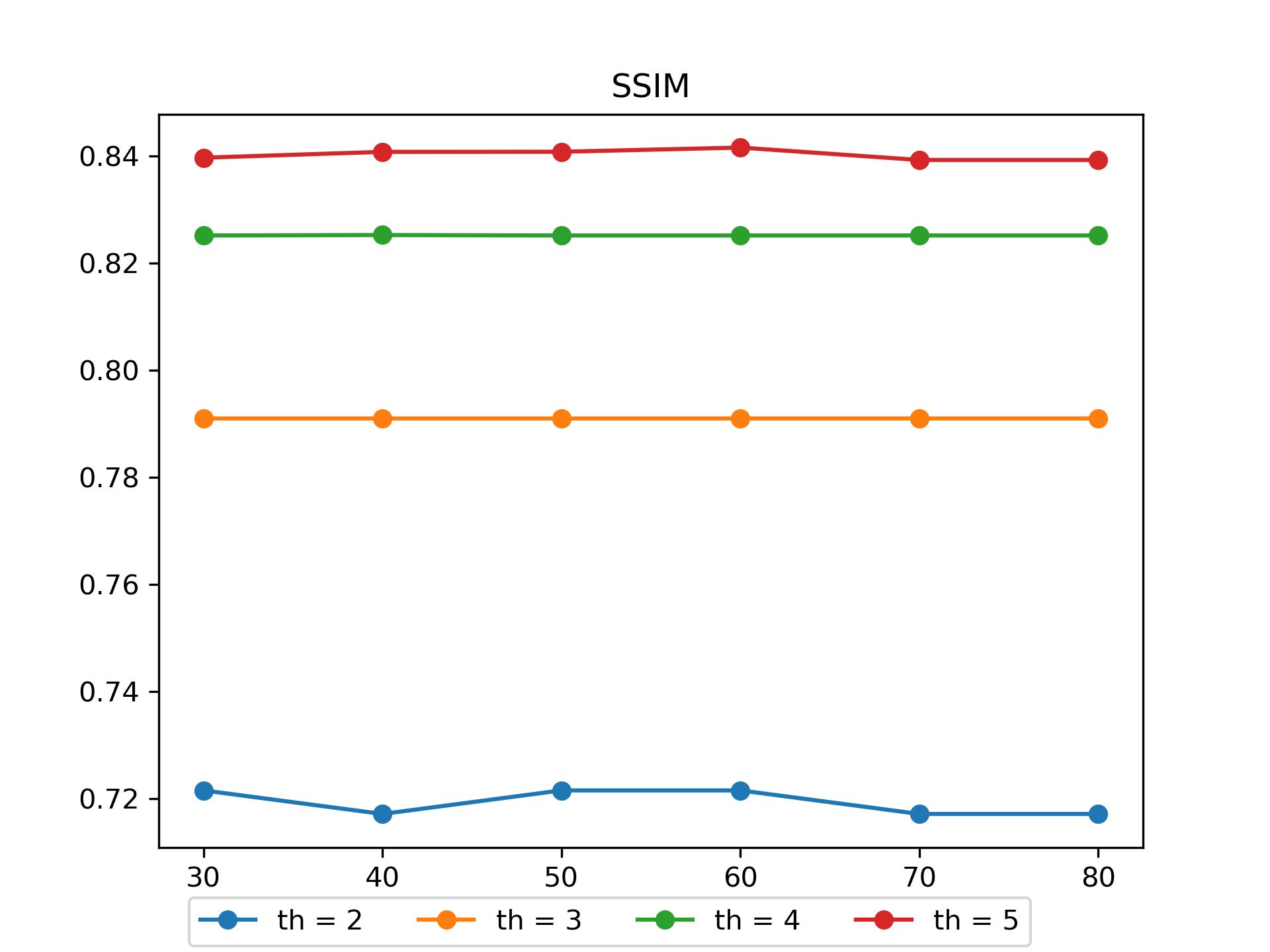
(h) Brainweb SSIM

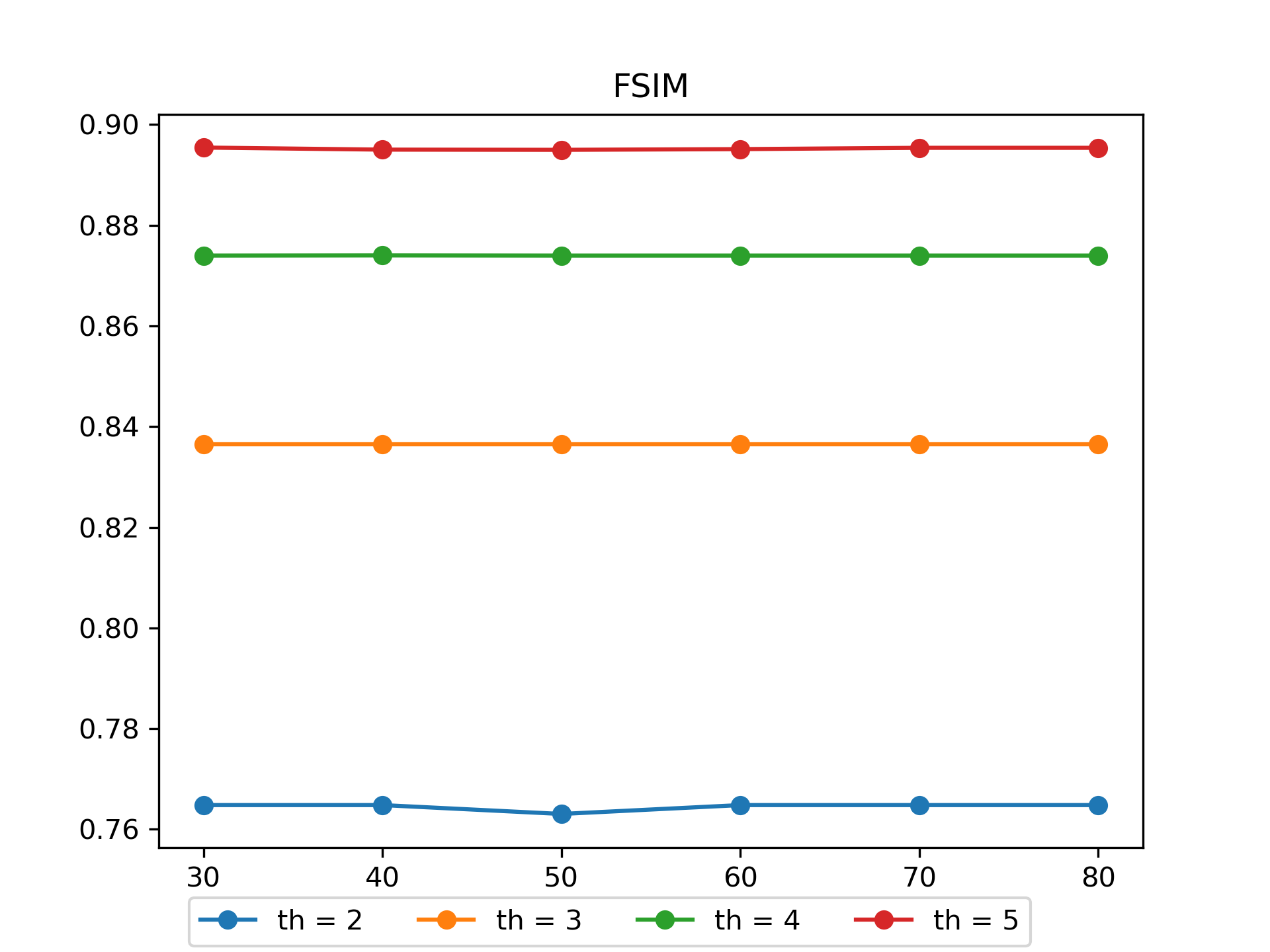
(i) Brainweb FSIM

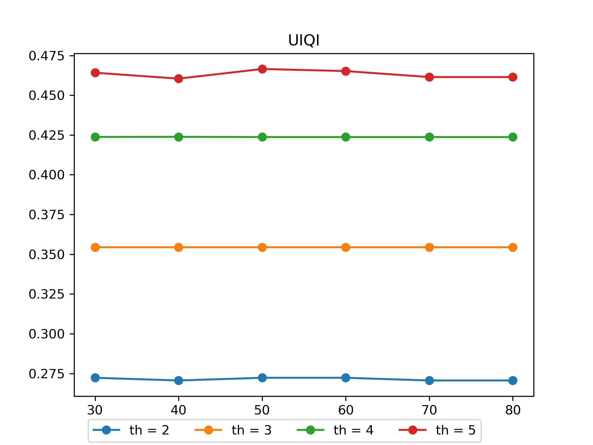
(j) Brainweb UIQI

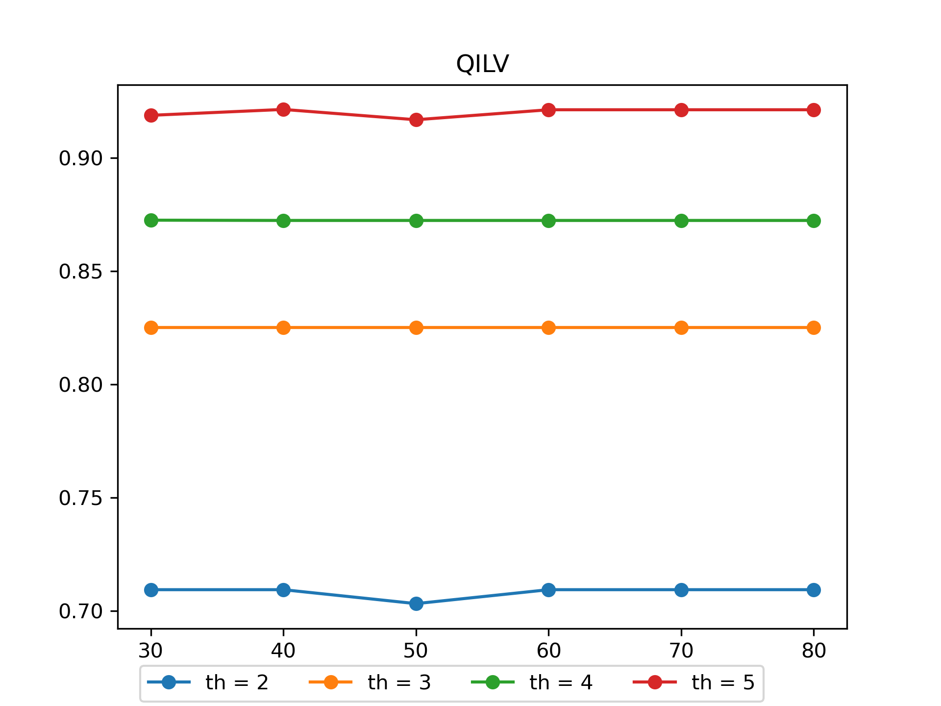
(k) Brainweb QILV

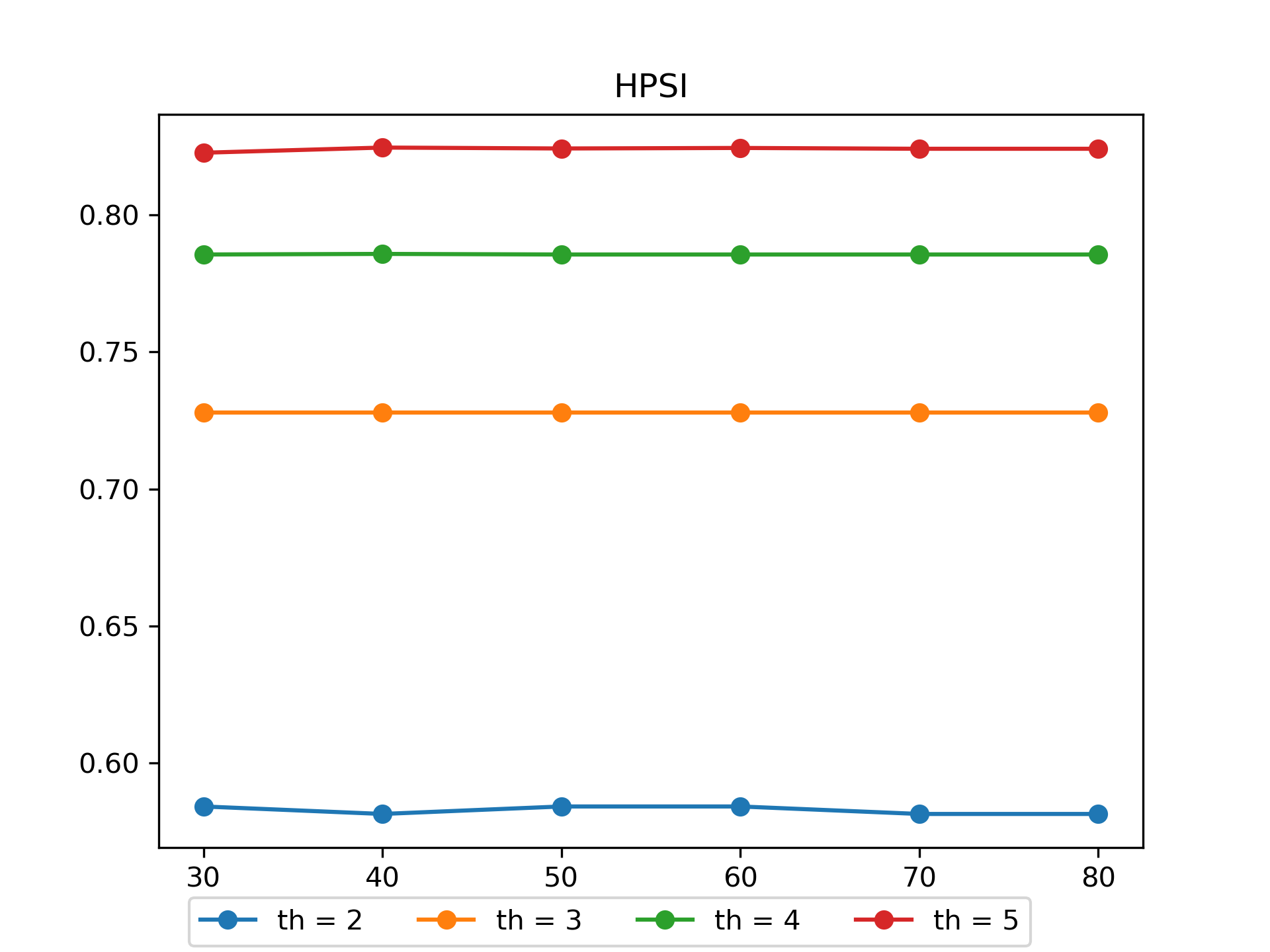
(l) Brainweb HPSI

Figure 10: Variation of performance with change in population size in HHO (altruism is set to 4 in each case): (a)-(f) in the Harvard WBA dataset; (g)-(l) in the Brainweb dataset.

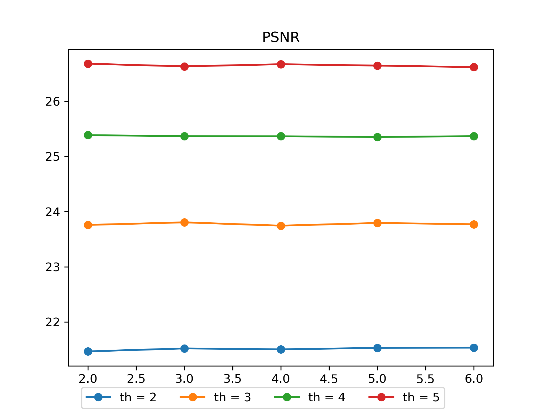
(a) Harvard PSNR

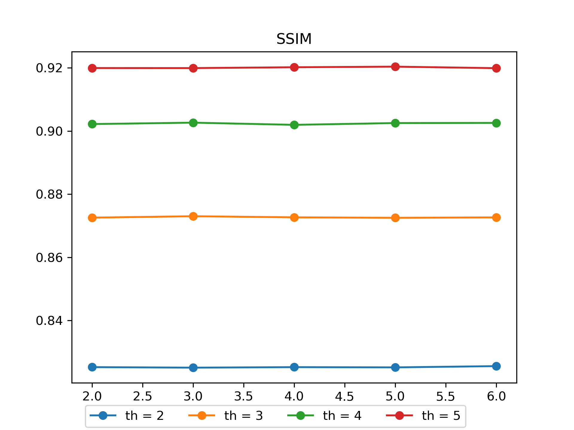
(b) Harvard SSIM

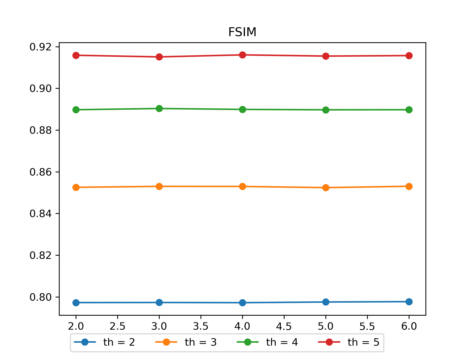
(c) Harvard FSIM

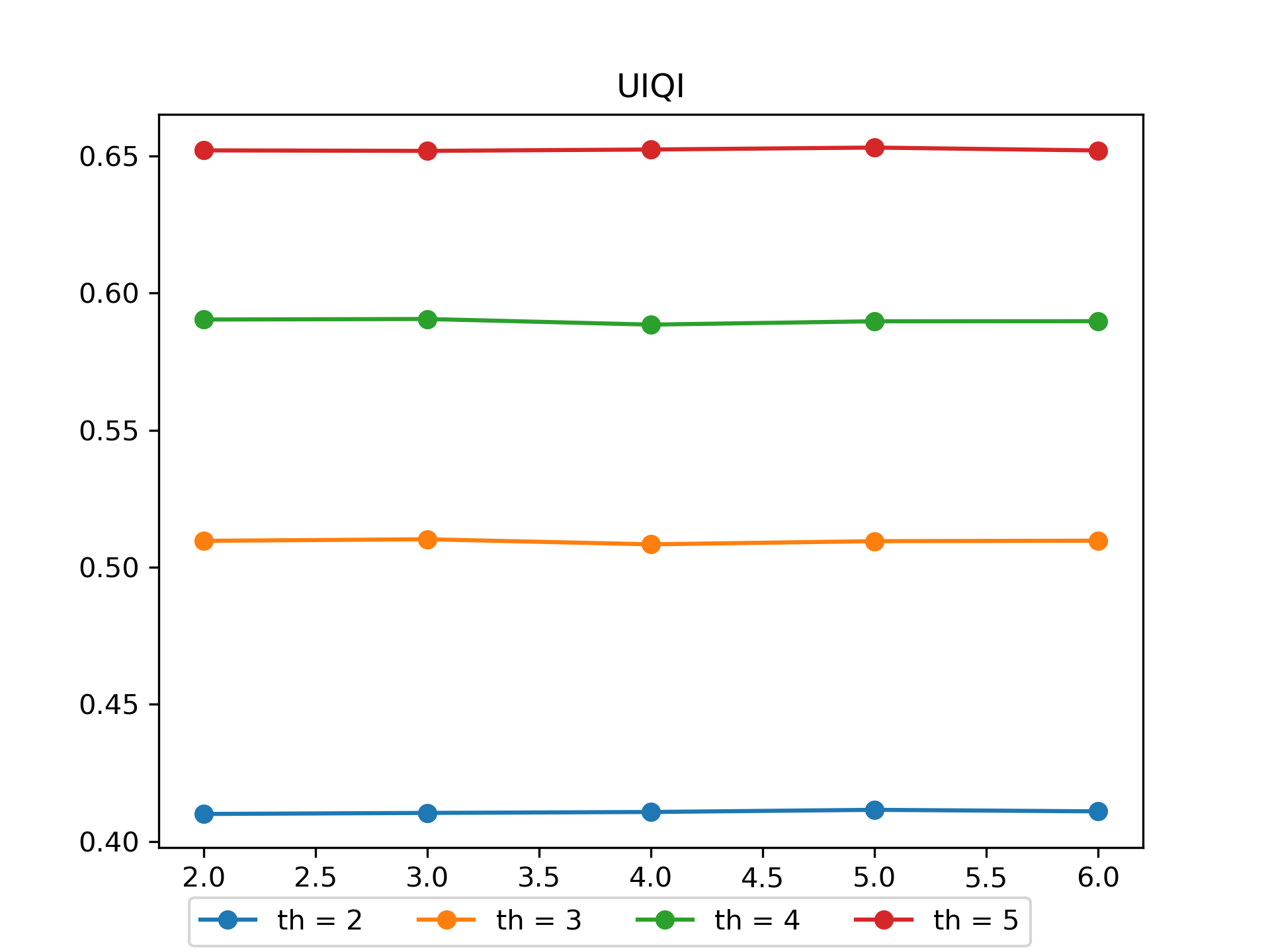
(d) Harvard UIQI

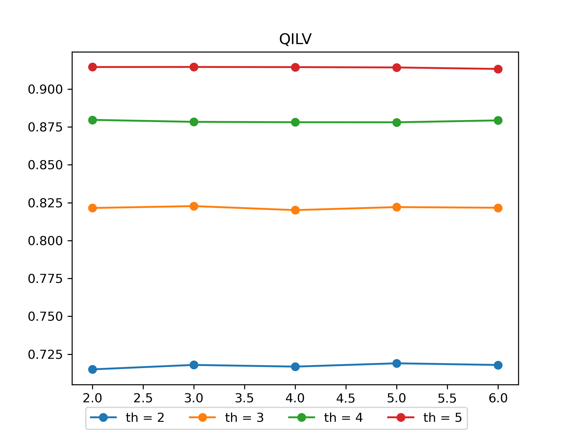
(e) Harvard QILV

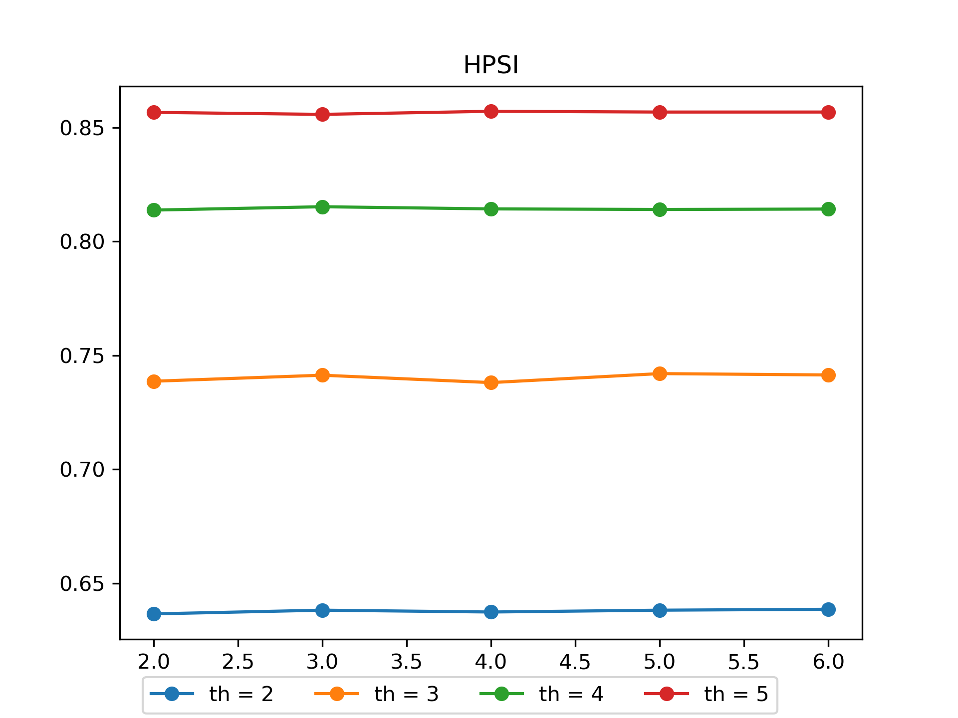
(f) Harvard HPSI

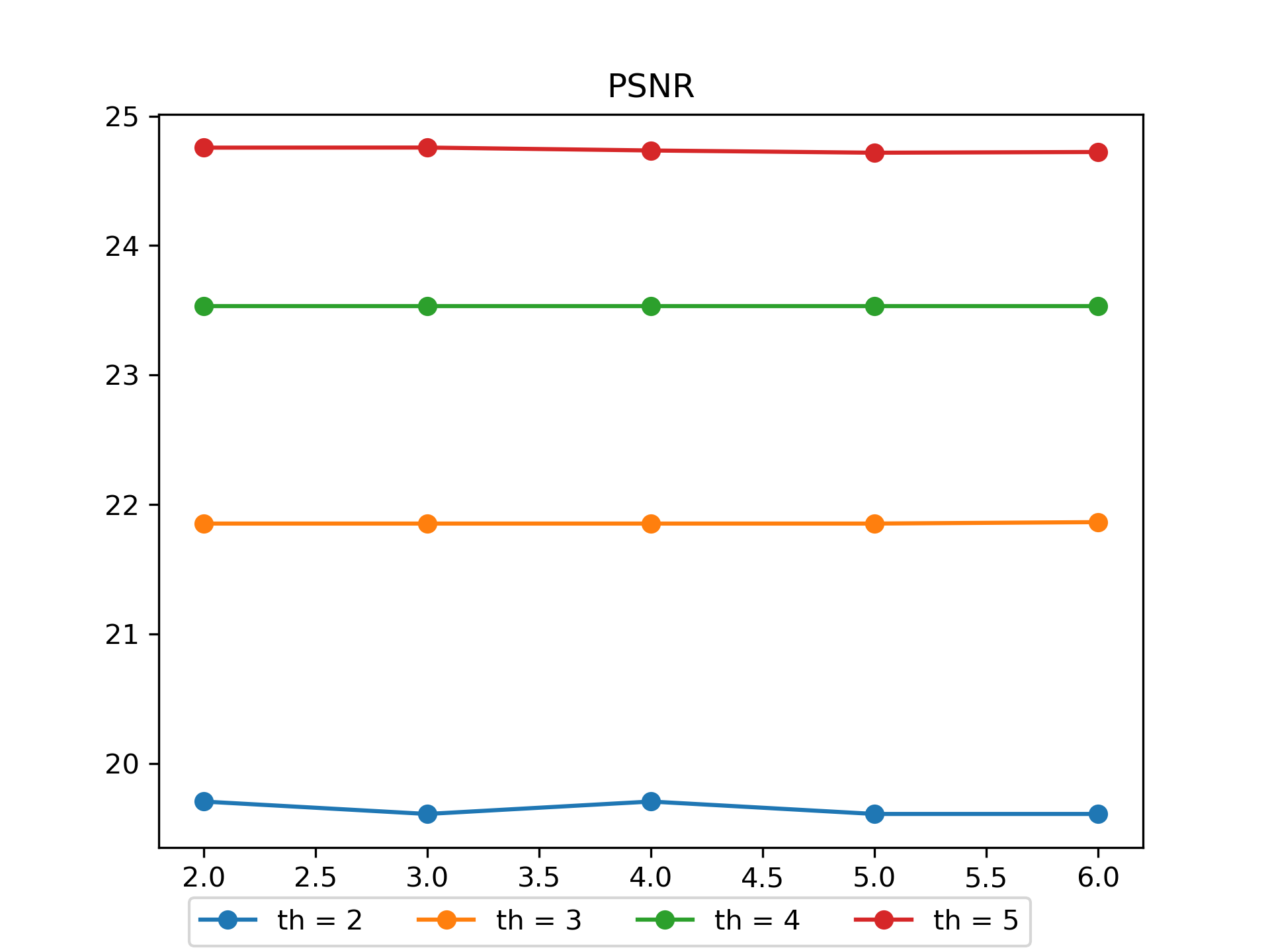
(g) Brainweb PSNR

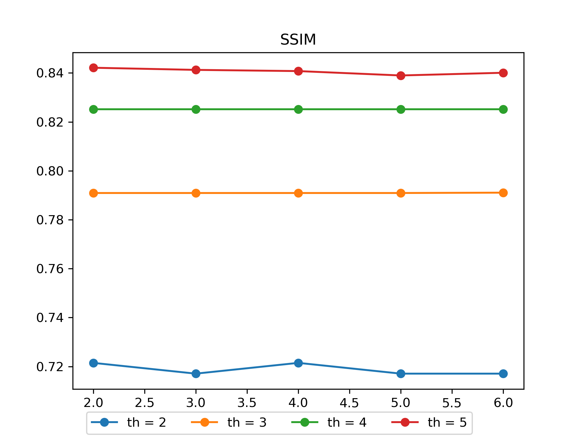
(h) Brainweb SSIM

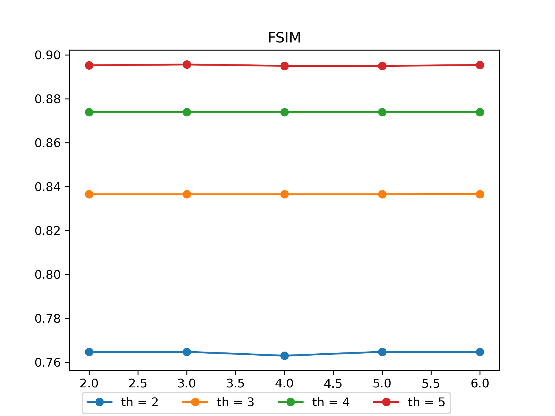
(i) Brainweb FSIM

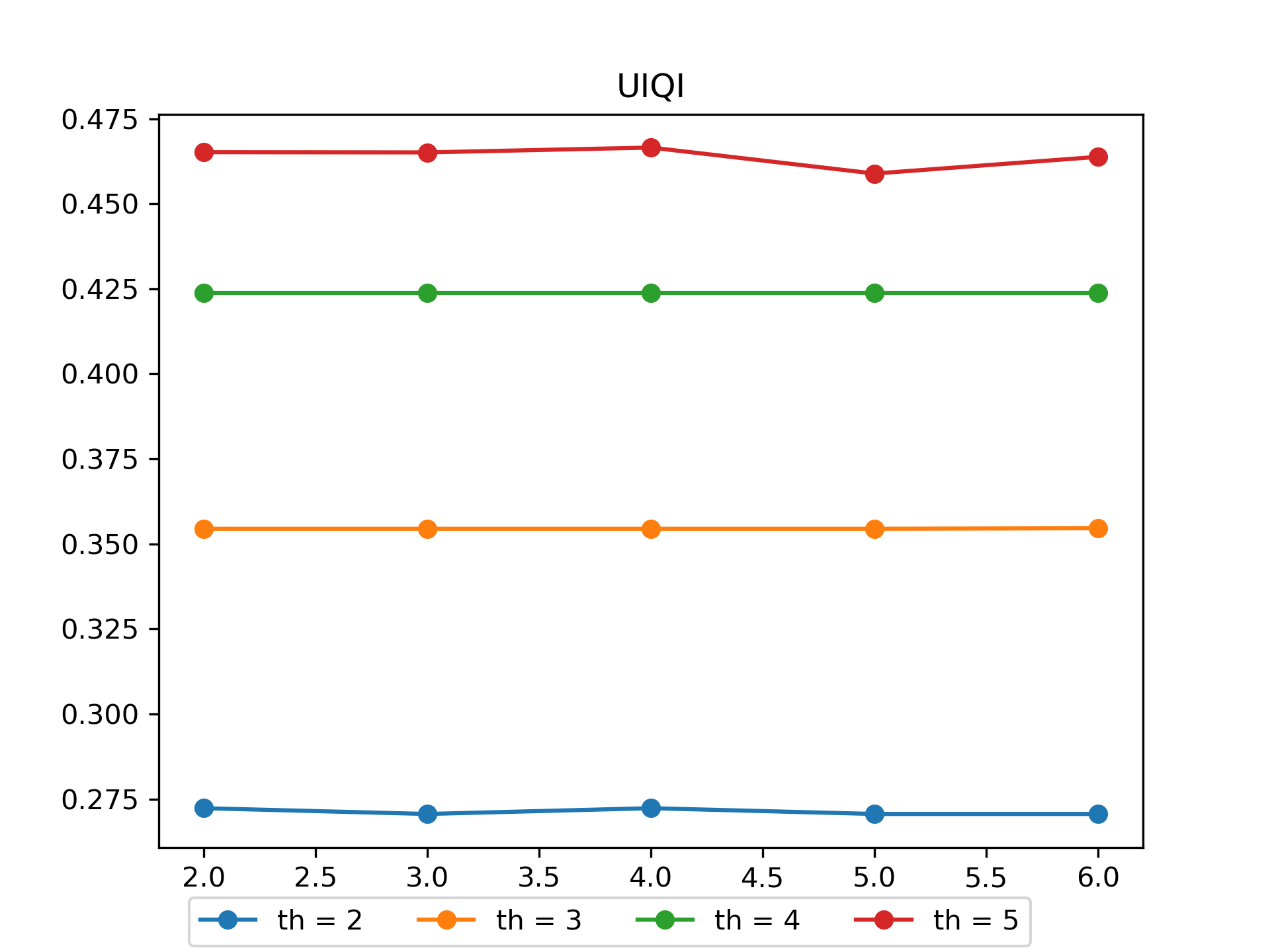
(j) Brainweb UIQI

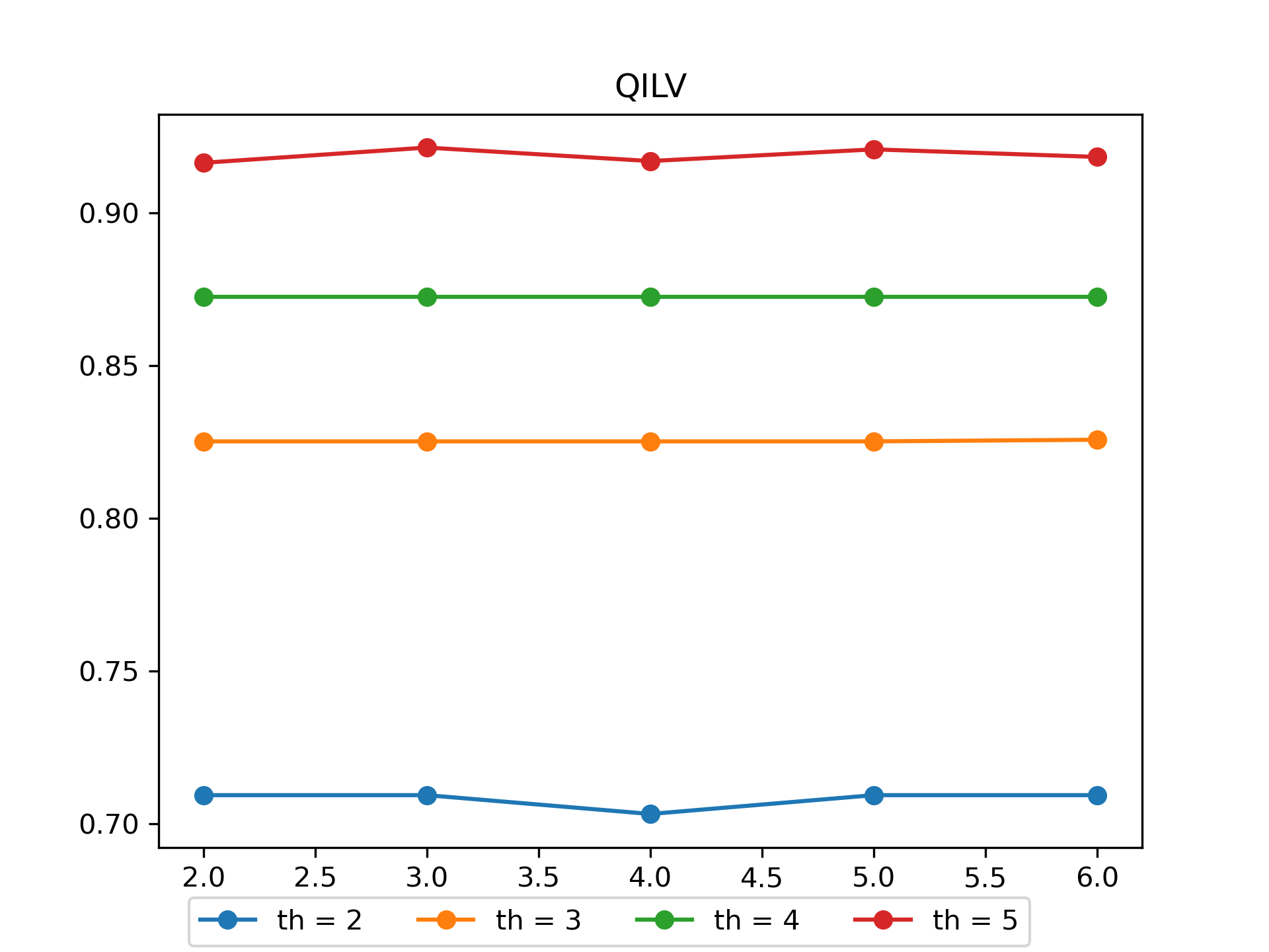
(k) Brainweb QILV

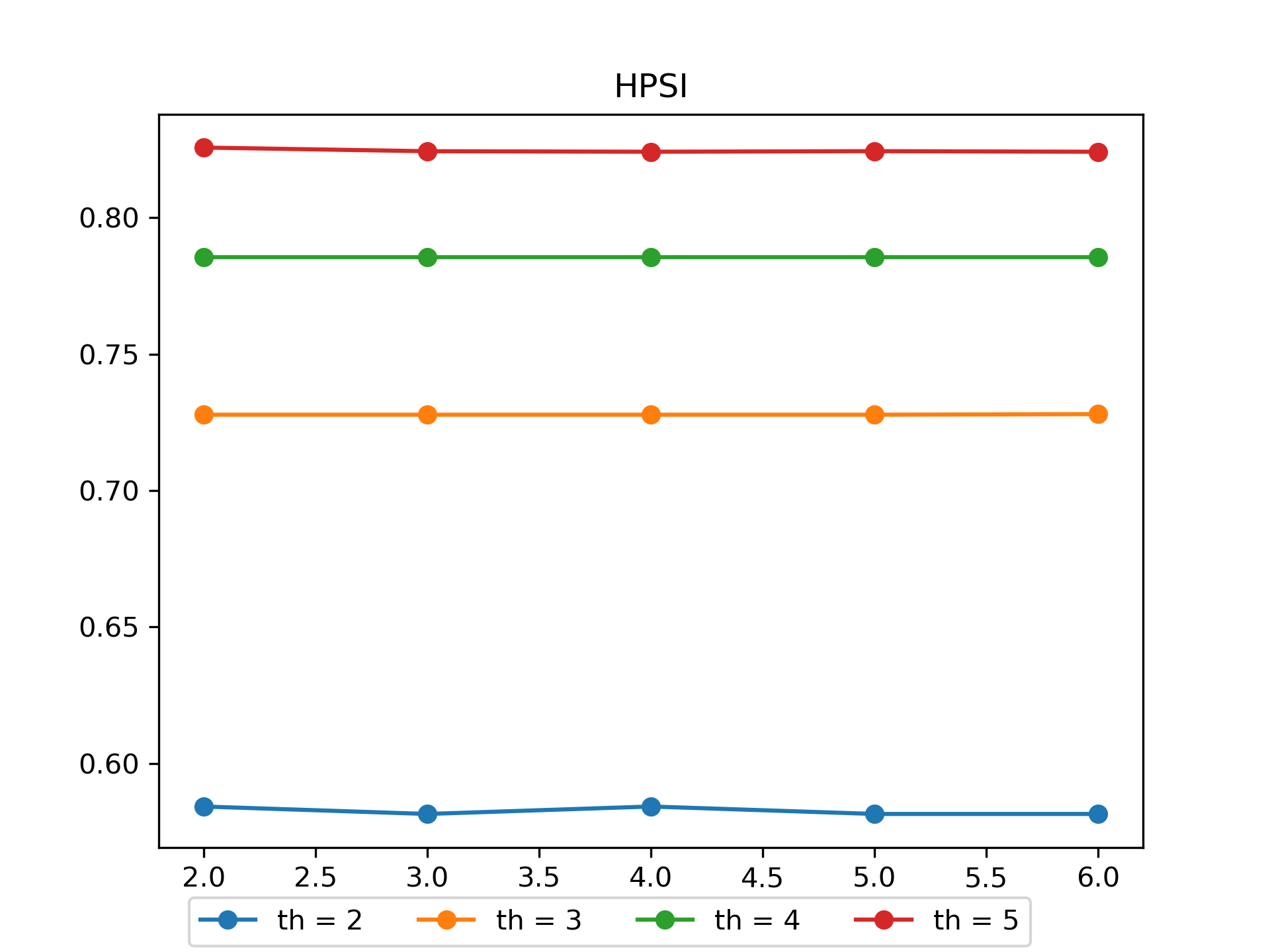
(l) Brainweb HPSI

Figure 11: Variation of performance with change in altruism in HHO (population is set to 50 in each case): (a)-(f) in the Harvard WBA dataset; (g)-(l) in the Brainweb dataset.

Figure 10 shows the variation in performance of the proposed framework with respect to the population size in the HHO algorithm. A population size of 50 gives consistently better results than the others, and hence 50 is chosen as the population in the algorithm framework.

Figure 11 shows the variation in performance of the proposed framework with respect to the number of altruistic individuals in the population of the HHO algorithm. Altruism when set to 4 (8% of population size) gives consistently better results than values higher or lower than 4, and hence it is chosen as the final altruism number in the algorithm for the final segmentation.

4.4 Comparison to state-of-the-art

Table 5: Comparison of the proposed method with other evolutionary algorithms for multi-level thresholding on the Harvard WBA database: the mean results from all 10 images are shown. The values in bold correspond to the best results obtained for the experiment.

Algorithm	No. of Thresholds	PSNR	SSIM	FSIM	UIQI	QILV	HPSI
	2	20.3954	0.8126	0.7629	0.3741	0.5691	0.5619
	3	22.5337	0.8638	0.8297	0.4967	0.7343	0.7000
	4	24.2621	0.8964	0.8700	0.5839	0.8190	0.7745
HHO [20]	5	25.6072	0.9196	0.8994	0.6503	0.8638	0.8312
	2	17.4848	0.7227	0.6675	0.4177	0.3336	0.2615
	3	20.3949	0.8122	0.7620	0.5599	0.5691	0.3743
	4	22.5438	0.8639	0.8289	0.6992	0.7366	0.4986
LSHADE [42]	5	24.3039	0.8973	0.8699	0.7746	0.8194	0.5851
	2	17.4334	0.7217	0.6648	0.4170	0.3292	0.2610
	3	20.3365	0.8117	0.7586	0.5588	0.5655	0.3736
	4	22.5043	0.8633	0.8272	0.6971	0.7344	0.4975
SADE [45]	5	24.2256	0.8965	0.8661	0.7702	0.8111	0.5771
	2	17.4246	0.7222	0.6671	0.4132	0.3283	0.2608
	3	20.3294	0.8115	0.7612	0.5584	0.5644	0.3726
	4	22.4584	0.8631	0.8281	0.6965	0.7319	0.4958
DE [14]	5	24.2290	0.8957	0.8669	0.7676	0.8158	0.5790
	2	17.4201	0.7217	0.6662	0.4156	0.3278	0.2604
	3	20.3303	0.8112	0.7600	0.5583	0.5620	0.3708
	4	22.4765	0.8617	0.8266	0.6952	0.7126	0.4893
PSO [28]	5	24.2359	0.8937	0.8672	0.7664	0.7832	0.5731
	2	17.4234	0.7220	0.6672	0.4173	0.3285	0.2608
	3	20.3357	0.8118	0.7612	0.5583	0.5644	0.3719
	4	22.4405	0.8622	0.8272	0.6928	0.7313	0.4938
GWO [35]	5	24.0956	0.8939	0.8644	0.7634	0.8092	0.5719
	2	17.2839	0.7003	0.6436	0.3400	0.2781	0.2315
	3	19.8034	0.7694	0.7108	0.4587	0.4467	0.3327
	4	21.1309	0.8132	0.7582	0.5444	0.5693	0.4121
SCA [46]	5	21.9658	0.8387	0.7892	0.6008	0.6478	0.4662
	2	20.3532	0.8127	0.7632	0.3741	0.5656	0.5621
	3	22.5069	0.8637	0.8297	0.4982	0.7339	0.7014
	4	24.1624	0.8968	0.8679	0.5755	0.8092	0.7684
WOA [34]	5	25.6927	0.9202	0.8996	0.6516	0.8658	0.8319
	2	20.3591	0.8123	0.7625	0.3738	0.5669	0.5615
	3	22.5495	0.8642	0.8304	0.4975	0.7348	0.7010
	4	24.2011	0.8966	0.8678	0.5773	0.8105	0.7714
ALO [30]	5	25.5824	0.9192	0.8992	0.6512	0.8634	0.8326
	2	20.3622	0.8121	0.7632	0.3736	0.5671	0.5616
	3	22.5093	0.8642	0.8302	0.4978	0.7332	0.7010
	4	24.2694	0.8965	0.8686	0.5801	0.8153	0.7725
MFO [31]	5	25.5434	0.9188	0.8988	0.6512	0.8628	0.8307
	2	20.3491	0.8124	0.7637	0.3732	0.5655	0.5621
	3	22.4844	0.8633	0.8300	0.4948	0.7328	0.6995
	4	24.2783	0.8969	0.8693	0.5813	0.8174	0.7737
DA [32]	5	25.5534	0.9187	0.8990	0.6480	0.8679	0.8327
	2	21.6240	0.8256	0.7977	0.4117	0.7223	0.6364
	3	23.7769	0.8722	0.8531	0.5091	0.8220	0.7399
	4	25.3682	0.9022	0.8902	0.5894	0.8784	0.8145
Proposed	5	26.6125	0.9197	0.9155	0.6515	0.9134	0.8570

Table 6: Comparison of the proposed method with other evolutionary algorithms for multi-level thresholding on the Brainweb database: the mean results from all 8 images used are shown. The values in bold correspond to the best results obtained for the experiment.

Algorithm	No. of Thresholds	PSNR	SSIM	FSIM	UIQI	QILV	HPSI
	2	18.8024	0.7158	0.7553	0.2720	0.6109	0.5665
	3	20.4756	0.7719	0.8151	0.3394	0.7542	0.7001
	4	22.3962	0.8236	0.8591	0.4125	0.8188	0.7720
HHO [20]	5	23.5675	0.8551	0.8857	0.4651	0.8520	0.8161
	2	18.8024	0.7158	0.7553	0.2720	0.6109	0.5665
	3	20.4756	0.7703	0.8151	0.3389	0.7542	0.7001
	4	22.2031	0.8244	0.8560	0.4075	0.8102	0.7685
LSHADE [42]	5	23.5619	0.8549	0.8856	0.4649	0.8519	0.8161
	2	18.7424	0.7058	0.7253	0.2520	0.5909	0.5465
	3	20.4156	0.7503	0.7851	0.3189	0.7242	0.6801
	4	22.1531	0.7944	0.8360	0.3875	0.7802	0.7485
SADE [45]	5	23.5219	0.8249	0.8656	0.4549	0.8319	0.7861
	2	18.7524	0.6958	0.7253	0.2520	0.5909	0.5365
	3	20.4356	0.7503	0.7951	0.3189	0.7342	0.6801
	4	22.1231	0.8044	0.8360	0.3875	0.7802	0.7485
DE [14]	5	23.4819	0.8449	0.8556	0.4349	0.8219	0.7961
	2	18.6986	0.7058	0.7319	0.2620	0.6009	0.5297
	3	20.3595	0.7469	0.8051	0.3289	0.7308	0.6901
	4	22.1239	0.7876	0.8326	0.3707	0.7734	0.7585
PSO [28]	5	23.4704	0.8449	0.8488	0.4549	0.8419	0.7927
	2	18.7411	0.6777	0.7306	0.2607	0.5996	0.5552
	3	20.3897	0.7322	0.7904	0.3142	0.7161	0.6754
	4	22.1295	0.8131	0.8313	0.3962	0.7989	0.7572
GWO [35]	5	23.5129	0.8436	0.8409	0.4402	0.8272	0.7780
	2	18.5496	0.6377	0.7240	0.1939	0.5796	0.5118
	3	20.3566	0.7390	0.7370	0.2842	0.6995	0.6454
	4	21.9280	0.7931	0.8247	0.3294	0.7789	0.7138
SCA [46]	5	23.3760	0.8236	0.8543	0.4336	0.7972	0.7380
	2	18.8024	0.7158	0.7553	0.2720	0.6109	0.5665
	3	20.4758	0.7703	0.8151	0.3389	0.7544	0.7001
	4	22.3490	0.8244	0.8584	0.4111	0.8155	0.7714
WOA [34]	5	23.5825	0.8549	0.8866	0.4659	0.8527	0.8161
	2	18.8024	0.7158	0.7553	0.2720	0.6109	0.5665
	3	20.4756	0.7703	0.8151	0.3389	0.7542	0.7001
	4	22.2978	0.8242	0.8577	0.4099	0.8139	0.7705
ALO [30]	5	23.5132	0.8549	0.8858	0.4649	0.8505	0.8149
	2	18.8024	0.7158	0.7553	0.2720	0.6109	0.5665
	3	20.4756	0.7703	0.8151	0.3389	0.7542	0.7001
	4	22.2978	0.8242	0.8577	0.4099	0.8139	0.7705
MFO [31]	5	23.5305	0.8539	0.8865	0.4617	0.8521	0.8147
	2	18.8040	0.7158	0.7553	0.2720	0.6115	0.5666
	3	20.5197	0.7709	0.8157	0.3392	0.7589	0.7019
	4	22.2008	0.8216	0.8551	0.4033	0.8155	0.7632
DA [32]	5	23.7499	0.8558	0.8882	0.4688	0.8611	0.8207
	2	19.6240	0.7176	0.7652	0.2711	0.7098	0.5818
	3	21.8767	0.7913	0.8368	0.3549	0.8258	0.7285
	4	23.5343	0.8251	0.8741	0.4237	0.8725	0.7857
Proposed	5	24.7686	0.8608	0.8959	0.4670	0.9192	0.8228

The following algorithms have been used to compare the results of the proposed method for brain MRI segmentation:

1. HHO (basic version) by [20]. The algorithm is inspired by the cooperative manner in which the Harris Hawks hunt in nature. They perform the surprise pounce to engulf the prey. Myriad chasing patterns can be emulated by this algorithm as discussed in our work.

2. L-SHADE by Piotrowski et al. [42] and utilized for brain MRI segmentation by Aranguren et al. [4] The main advantage of using L-SHADE as a meta-heuristic is that the parameters internal to the algorithm are tuned according to the information that is acquired during the process of evolution. The latter has used LSHADE to perform multi-level thresholding, using the minimum cross-entropy function as the objective function.

3. Differential Evolution (DE) by Price et al. [14]. DE is a powerful meta-heuristic and its application to multi-objective and large scale problems have been demonstrated.

4. Self-Adaptive Differential Evolution (SADE) by [45]. SADE The trial vector generation techniques, as well as the control values of parameters, are adapted by the algorithm itself using its past experiences. The performance is evaluated on constrained optimization problems, and comparison has been drawn with the other variants of adaptive DE

5. Particle Swarm Optimization (PSO) by Marini et al. [28] The solution is taken to be a swarm of particles. The prowess of the algorithm has been demonstrated in solving optimization problems, particularly in chemometrics.

6. Grey Wolf Optimization (GWO) by Mirjalili et al. [35] It imitates how the grey wolves hunt in nature. It performs well on the unimodal functions. And the good results on the multimodal functions support the exploration capability of the GWO. It yields superior results on real problems as well

7. Sine-Cosine Algorithm (SCA) by Mirjalili et al. [33]. Initially, random solutions are there and gradually they fluctuate away from or move towards the optimal solution according to a pre-defined mathematical model that deploys sine and cosine functions. The method is tested on unimodal, multi-modal and composite functions, and, on two-dimensional test functions.

8. Whale Optimization Algorithm (WOA) by Mirjalili et al. [34]. It is primarily encouraged by the humpback whales, and specifically the bubble-net hunting approach. It is tested on some of the benchmarked test functions, as well as on unimodal and multimodal functions.

9. Ant Lion Optimizer (ALO) by Mirjalili et al. [30] It is encouraged by how the antlions hunt and is tested on unimodal, multimodal, and benchmarked test functions as well as real problems.

10. Moth-Flame Optimization Algorithm (MFO) by Mirjalili et al. [31] It is influenced by how moths navigate, and specifically, the transverse orientation. It is evaluated on the benchmarked problems, as well as some real engineering problems and delivers superior results. The algorithm has been considered for application in the domain of marine propeller design.

11. Dragonfly Algorithm by Mirjalili (DA) by Mirjalili et al. [32] It is encouraged by how the dragonflies in nature swarm, namely, static and dynamic. Binary and multi-objective models of DA have been considered. Both of these have been tested on a real case study and myriad test functions.

For the algorithms, including the proposed algorithm, which require us to set the population size, the population size is set at 50. The maximum number of iterations is set at 1000 for all of the algorithms, the lower bound is set at 1 and the upper bound at 256. The parameters set for the state of the art algorithms are tabulated in Table 7. The names of the parameters have been taken from the commonly used literature. Apart from this, any other parameters not mentioned explicitly in Table 7 are also taken up directly from the established literature.

Table 7: Parameter tuning settings of the other state-of-the-art algorithms

Algorithm	Parameters
SADE	$learn\_generations=50$
	$rate\_crossover=0.50$
DE	$value\_scale_{f}actor=0.20$
	$init\_population\_size=50$
	$final\_population\_size=40$
LSHADE	$memory\_size=5$
GWO	$a$ is in range $[2,0]$
PSO	$value\_weight$ is in range $[1,0]$
WOA	$a$ is in range $[2,0]$
	$a=3$
SCA	$value\_r1$ is in range $[1,0]$
	$convergence\_const$ is in range $[-1,-2]$
MFO	$value\_spiral\_factor=1$
ALO	No additional parameters
DA	No additional parameters

The comparative results are shown in Table 5 for the images taken from Harvard WBA database images, and in Table 6 for the images taken from the Brainweb dataset. As evident from the comparative results, the proposed approach outperforms the other evolutionary metaheuristic algorithms by a significant margin. The values shown in the table are determined by averaging the metrics we get by running the algorithms over all the images of each dataset. It is seen that for each of the metrics, we get a significant increment using Altruism with the HHO algorithm. It is observed that for the images in the Harvard WBA database, the performance delivered by WOA is closest to the proposed approach. HHO, ALO, MFO and DA yielded values that were somewhat close to the WOA. However, there is a clear gap between the values yielded by these algorithms and the proposed method. For the Brainweb dataset, it is observed that the performance of the DA is closest to the proposed method. Some other algorithms such as HHO, L-SHADE and WOA also yield values close to the values obtained by the DA. However, the proposed algorithm outperforms these methods by a significant margin.

4.5 Findings of the work:

The findings of the work can be summarized as:

1. Evaluation of the proposed algorithm on MRI images from the WBA database developed by Harvard Medical School and the Brainweb database.

2. Use of six metrics for evaluating the performance which are: PSNR, SSIM, FSIM, HPSI, QILV, UIQI.

3. Performed experiments using different threshold values for multi-level thresholding.

4. Output images are provided to show the qualitative results on both of the datasets. The original image is placed with the thresholded images for viewing the difference between the images.

5. Compared the performances of the various chaotic maps and selected the Logistic chaotic map which delivers the best results amongst the chaotic maps.

6. Evaluated the performance of the proposed algorithm using various objective functions and demonstrated the superior performance of the proposed objective function.

7. Tuned the hyperparameters of the algorithm such as the population size and value of the parameter in altruism to get the best results.

8. Compared the performance of the proposed algorithm with other meta-heuristic algorithms such as L-SHADE, SADE, DE, PSO, GWO, SCA, WOA, ALO, MFO and DA to justify the good performance of the proposed algorithm.

5 Conclusions

Segmentation is an important preprocessing step in medical image analysis. Brain MRI segmentation is essential for disease identification, lesion delineation and better visualization of morphological changes. In this research, we explore the unsupervised segmentation of brain MRI images using a multi-level thresholding approach. Classical methods like Otsu’s thresholding, or Kapur’s entropy-based methods are inefficient for segmentation using a large number of thresholds, thus we explore evolutionary optimization algorithms to approach this problem. For this, we use an improved Harris Hawks Optimization algorithm wherein we embed the concept of altruism and use a hybrid of two objective functions. As evident from the results, HHO incorporated with altruism to enhance its exploitation capability, chaotic initialization to increase the diversity of the solutions and the hybrid objective function, yields results whose performance metrics are significantly better than the meta-heuristics that have been used earlier. The limitations of the feature selection algorithm have been mitigated to some extent by integrating altruism and a Logistic chaotic map. We evaluate the proposed algorithm on T2-weighted brain MRIs extracted from two popular publicly available databases: the Harvard WBA and the Brainweb datasets. Upon comparison, it is established that the proposed framework outperforms state-of-the-art methods on the same datasets, thus justifying the effectiveness of the model.

The main limitation of the proposed algorithm is that it consumes more time compared to other meta-heuristics due to the time complexity of the HHO algorithm and the altruism integrated into it. A balance can however be established between the time taken by the algorithm and the values of the performance metrics by decreasing the number of search agents or decreasing the number of iterations inside the feature selection algorithm. Future work will focus on overcoming these limitations and further increase the exploitation capability of the algorithm.

Conflict of interest

All the authors declare that there is no conflict of interest.

References

- Abutaleb [1989] Abutaleb, A. S. (1989). Automatic thresholding of gray-level pictures using two-dimensional entropy. Computer vision, graphics, and image processing, 47, 22–32.
- Aja-Fernandez et al. [2006] Aja-Fernandez, S., Estepar, R. S. J., Alberola-Lopez, C., & Westin, C.-F. (2006). Image quality assessment based on local variance. In 2006 international conference of the ieee engineering in medicine and biology society (pp. 4815–4818). IEEE.
- Akay [2013] Akay, B. (2013). A study on particle swarm optimization and artificial bee colony algorithms for multilevel thresholding. Applied Soft Computing, 13, 3066–3091.
- Aranguren et al. [2021] Aranguren, I., Valdivia, A., Morales-Castañeda, B., Oliva, D., Abd Elaziz, M., & Perez-Cisneros, M. (2021). Improving the segmentation of magnetic resonance brain images using the lshade optimization algorithm. Biomedical Signal Processing and Control, 64, 102259.
- Askarzadeh [2016] Askarzadeh, A. (2016). A novel metaheuristic method for solving constrained engineering optimization problems: crow search algorithm. Computers & Structures, 169, 1–12.
- Avcıbas et al. [2002] Avcıbas, I., Sankur, B., & Sayood, K. (2002). Statistical evaluation of image quality measures. Journal of Electronic Imaging, 11, 206–223.
- Baur et al. [2021] Baur, C., Wiestler, B., Muehlau, M., Zimmer, C., Navab, N., & Albarqouni, S. (2021). Modeling healthy anatomy with artificial intelligence for unsupervised anomaly detection in brain mri. Radiology: Artificial Intelligence, 3, e190169.
- Bednarz [1988] Bednarz, J. C. (1988). Cooperative hunting harris’ hawks (parabuteo unicinctus). Science, 239, 1525–1527.
- Bercea et al. [2021] Bercea, C. I., Wiestler, B., Rueckert, D., & Albarqouni, S. (2021). Feddis: Disentangled federated learning for unsupervised brain pathology segmentation. arXiv preprint arXiv:2103.03705, .
- Cai et al. [2021] Cai, X., Zhao, H., Shang, S., Zhou, Y., Deng, W., Chen, H., & Deng, W. (2021). An improved quantum-inspired cooperative co-evolution algorithm with muli-strategy and its application. Expert Systems with Applications, 171, 114629.
- Chang & Wang [1997] Chang, C.-C., & Wang, L.-L. (1997). A fast multilevel thresholding method based on lowpass and highpass filtering. Pattern Recognition Letters, 18, 1469–1478.
- Cho et al. [1989] Cho, S., Haralick, R., & Yi, S. (1989). Improvement of kittler and illingworth’s minimum error thresholding. Pattern Recognition, 22, 609–617.
- Cocosco et al. [1997] Cocosco, C. A., Kollokian, V., Kwan, R. K.-S., Pike, G. B., & Evans, A. C. (1997). Brainweb: Online interface to a 3d mri simulated brain database. In NeuroImage. Citeseer.
- Das & Suganthan [2010] Das, S., & Suganthan, P. N. (2010). Differential evolution: A survey of the state-of-the-art. IEEE transactions on evolutionary computation, 15, 4–31.
- Deng et al. [2021] Deng, W., Shang, S., Cai, X., Zhao, H., Zhou, Y., Chen, H., & Deng, W. (2021). Quantum differential evolution with cooperative coevolution framework and hybrid mutation strategy for large scale optimization. Knowledge-Based Systems, (p. 107080).
- Deng et al. [2020a] Deng, W., Xu, J., Gao, X.-Z., & Zhao, H. (2020a). An enhanced msiqde algorithm with novel multiple strategies for global optimization problems. IEEE Transactions on Systems, Man, and Cybernetics: Systems, .
- Deng et al. [2020b] Deng, W., Xu, J., Zhao, H., & Song, Y. (2020b). A novel gate resource allocation method using improved pso-based qea. IEEE Transactions on Intelligent Transportation Systems, .
- Ewees & Elaziz [2020] Ewees, A. A., & Elaziz, M. A. (2020). Performance analysis of chaotic multi-verse harris hawks optimization: A case study on solving engineering problems. Engineering Applications of Artificial Intelligence, 88, 103370. URL: https://doi.org/10.1016/j.engappai.2019.103370. doi:10.1016/j.engappai.2019.103370.
- Feng et al. [2017] Feng, Y., Zhao, H., Li, X., Zhang, X., & Li, H. (2017). A multi-scale 3d otsu thresholding algorithm for medical image segmentation. Digital Signal Processing, 60, 186–199.
- Heidari et al. [2019] Heidari, A. A., Mirjalili, S., Faris, H., Aljarah, I., Mafarja, M., & Chen, H. (2019). Harris hawks optimization: Algorithm and applications. Future generation computer systems, 97, 849–872.
- Kadry et al. [2021] Kadry, S., Rajinikanth, V., Raja, N. S. M., Hemanth, D. J., Hannon, N. M., & Raj, A. N. J. (2021). Evaluation of brain tumor using brain mri with modified-moth-flame algorithm and kapur’s thresholding: a study. Evolutionary Intelligence, 14, 1053–1063.
- Kapur et al. [1985] Kapur, J. N., Sahoo, P. K., & Wong, A. K. (1985). A new method for gray-level picture thresholding using the entropy of the histogram. Computer vision, graphics, and image processing, 29, 273–285.
- Kaur et al. [2016] Kaur, T., Saini, B. S., & Gupta, S. (2016). Optimized multi threshold brain tumor image segmentation using two dimensional minimum cross entropy based on co-occurrence matrix. In Medical imaging in clinical applications (pp. 461–486). Springer.
- Kittler & Illingworth [1986] Kittler, J., & Illingworth, J. (1986). Minimum error thresholding. Pattern recognition, 19, 41–47.
- Kullback [1997] Kullback, S. (1997). Information theory and statistics. Courier Corporation.
- Lai & Tseng [2004] Lai, C.-C., & Tseng, D.-C. (2004). A hybrid approach using gaussian smoothing and genetic algorithm for multilevel thresholding. International Journal of Hybrid Intelligent Systems, 1, 143–152.
- Li & Lee [1993] Li, C. H., & Lee, C. (1993). Minimum cross entropy thresholding. Pattern recognition, 26, 617–625.
- Marini & Walczak [2015] Marini, F., & Walczak, B. (2015). Particle swarm optimization (pso). a tutorial. Chemometrics and Intelligent Laboratory Systems, 149, 153–165.
- Menesy et al. [2020] Menesy, A. S., Sultan, H. M., Selim, A., Ashmawy, M. G., & Kamel, S. (2020). Developing and applying chaotic harris hawks optimization technique for extracting parameters of several proton exchange membrane fuel cell stacks. IEEE Access, 8, 1146–1159. URL: https://doi.org/10.1109/access.2019.2961811. doi:10.1109/access.2019.2961811.
- Mirjalili [2015a] Mirjalili, S. (2015a). The ant lion optimizer. Advances in engineering software, 83, 80–98.
- Mirjalili [2015b] Mirjalili, S. (2015b). Moth-flame optimization algorithm: A novel nature-inspired heuristic paradigm. Knowledge-based systems, 89, 228–249.
- Mirjalili [2016a] Mirjalili, S. (2016a). Dragonfly algorithm: a new meta-heuristic optimization technique for solving single-objective, discrete, and multi-objective problems. Neural Computing and Applications, 27, 1053–1073.
- Mirjalili [2016b] Mirjalili, S. (2016b). Sca: a sine cosine algorithm for solving optimization problems. Knowledge-based systems, 96, 120–133.
- Mirjalili & Lewis [2016] Mirjalili, S., & Lewis, A. (2016). The whale optimization algorithm. Advances in engineering software, 95, 51–67.
- Mirjalili et al. [2014] Mirjalili, S., Mirjalili, S. M., & Lewis, A. (2014). Grey wolf optimizer. Advances in engineering software, 69, 46–61.
- Oliva et al. [2019] Oliva, D., Abd Elaziz, M., & Hinojosa, S. (2019). Multilevel thresholding for image segmentation based on metaheuristic algorithms. In Metaheuristic Algorithms for Image Segmentation: Theory and Applications (pp. 59–69). Springer.
- Oliva et al. [2017] Oliva, D., Hinojosa, S., Cuevas, E., Pajares, G., Avalos, O., & Gálvez, J. (2017). Cross entropy based thresholding for magnetic resonance brain images using crow search algorithm. Expert Systems with Applications, 79, 164–180.
- Oliva et al. [2020] Oliva, D., Martins, M. S., Osuna-Enciso, V., & de Morais, E. F. (2020). Combining information from thresholding techniques through an evolutionary bayesian network algorithm. Applied Soft Computing, 90, 106147.
- Otsu [1979] Otsu, N. (1979). A threshold selection method from gray-level histograms. IEEE transactions on systems, man, and cybernetics, 9, 62–66.
- Panda et al. [2021] Panda, R., Samantaray, L., Das, A., Agrawal, S., & Abraham, A. (2021). A novel evolutionary row class entropy based optimal multi-level thresholding technique for brain mr images. Expert Systems with Applications, 168, 114426.
- Pham et al. [2000] Pham, D. L., Xu, C., & Prince, J. L. (2000). Current methods in medical image segmentation. Annual review of biomedical engineering, 2, 315–337.
- Piotrowski [2018] Piotrowski, A. P. (2018). L-shade optimization algorithms with population-wide inertia. Information Sciences, 468, 117–141.
- Prudkov & Rodina [2016] Prudkov, P. N., & Rodina, O. N. (2016). On altruism toward nonhuman animals. Society & Animals, 24, 321–336.
- Pun [1980] Pun, T. (1980). A new method for grey-level picture thresholding using the entropy of the histogram. Signal processing, 2, 223–237.
- Qin et al. [2008] Qin, A. K., Huang, V. L., & Suganthan, P. N. (2008). Differential evolution algorithm with strategy adaptation for global numerical optimization. IEEE transactions on Evolutionary Computation, 13, 398–417.
- Qu et al. [2018] Qu, C., Zeng, Z., Dai, J., Yi, Z., & He, W. (2018). A modified sine-cosine algorithm based on neighborhood search and greedy levy mutation. Computational Intelligence and Neuroscience, 2018.
- Ramakrishnan & Sankaragomathi [2017] Ramakrishnan, T., & Sankaragomathi, B. (2017). A professional estimate on the computed tomography brain tumor images using svm-smo for classification and mrg-gwo for segmentation. Pattern Recognition Letters, 94, 163–171.
- Reisenhofer et al. [2018] Reisenhofer, R., Bosse, S., Kutyniok, G., & Wiegand, T. (2018). A haar wavelet-based perceptual similarity index for image quality assessment. Signal Processing: Image Communication, 61, 33–43.
- Rodriguez-Esparza et al. [2020] Rodriguez-Esparza, E., Zanella-Calzada, L. A., Oliva, D., Heidari, A. A., Zaldivar, D., Pérez-Cisneros, M., & Foong, L. K. (2020). An efficient harris hawks-inspired image segmentation method. Expert Systems with Applications, 155, 113428.
- Sathya & Kayalvizhi [2011] Sathya, P., & Kayalvizhi, R. (2011). Optimal segmentation of brain mri based on adaptive bacterial foraging algorithm. Neurocomputing, 74, 2299–2313.
- Sims et al. [2008] Sims, D. W., Southall, E. J., Humphries, N. E., Hays, G. C., Bradshaw, C. J. A., Pitchford, J. W., James, A., Ahmed, M. Z., Brierley, A. S., Hindell, M. A., Morritt, D., Musyl, M. K., Righton, D., Shepard, E. L. C., Wearmouth, V. J., Wilson, R. P., Witt, M. J., & Metcalfe, J. D. (2008). Scaling laws of marine predator search behaviour. Nature, 451, 1098–1102. URL: https://doi.org/10.1038/nature06518. doi:10.1038/nature06518.
- Singh & Bala [2021] Singh, C., & Bala, A. (2021). An unsupervised orthogonal rotation invariant moment based fuzzy c-means approach for the segmentation of brain magnetic resonance images. Expert Systems with Applications, 164, 113989.
- Singh et al. [2021] Singh, S., Mittal, N., Thakur, D., Singh, H., Oliva, D., & Demin, A. (2021). Nature and biologically inspired image segmentation techniques. Archives of Computational Methods in Engineering, (pp. 1–28).
- Song et al. [2021] Song, Y., Wu, D., Deng, W., Gao, X.-Z., Li, T., Zhang, B., & Li, Y. (2021). Mppcede: multi-population parallel co-evolutionary differential evolution for parameter optimization. Energy Conversion and Management, 228, 113661.
- Stich et al. [2010] Stich, S., Doris, J. M., & Roedder, E. (2010). Altruism. American Physiological Association, .
- Sutton [1999] Sutton, D. (1999). The whole brain atlas.
- Tang et al. [2017] Tang, K., Xiao, X., Wu, J., Yang, J., & Luo, L. (2017). An improved multilevel thresholding approach based modified bacterial foraging optimization. Applied Intelligence, 46, 214–226.
- Viswanathan et al. [2000] Viswanathan, G., Afanasyev, V., Buldyrev, S. V., Havlin, S., da Luz, M., Raposo, E., & Stanley, H. (2000). Lévy flights in random searches. Physica A: Statistical Mechanics and its Applications, 282, 1–12. URL: https://doi.org/10.1016/s0378-4371(00)00071-6. doi:10.1016/s0378-4371(00)00071-6.
- Waibel et al. [2011] Waibel, M., Floreano, D., & Keller, L. (2011). A quantitative test of hamilton’s rule for the evolution of altruism. PLoS Biol, 9, e1000615.
- Wang & Bovik [2002] Wang, Z., & Bovik, A. C. (2002). A universal image quality index. IEEE signal processing letters, 9, 81–84.
- Wang et al. [2004] Wang, Z., Bovik, A. C., Sheikh, H. R., & Simoncelli, E. P. (2004). Image quality assessment: from error visibility to structural similarity. IEEE transactions on image processing, 13, 600–612.
- Yang [2010] Yang, X.-S. (2010). Nature-inspired metaheuristic algorithms. Luniver press.
- Yin [1999] Yin, P.-Y. (1999). A fast scheme for optimal thresholding using genetic algorithms. Signal processing, 72, 85–95.
- Zhang et al. [2011] Zhang, L., Zhang, L., Mou, X., & Zhang, D. (2011). Fsim: A feature similarity index for image quality assessment. IEEE transactions on Image Processing, 20, 2378–2386.