Thermalization in one-dimensional chains: the role of asymmetry and nonlinearity

Abstract

The symmetry of interparticle interaction potential (IIP) has a crucial influence on the thermodynamic and transport properties of solids. Here we focus on the effect of the asymmetry of IIP on thermalization properties. In general, asymmetry and nonlinearity interweave with each other. To explore the effects of asymmetry and nonlinearity on thermalization separately, we here introduce an asymmetric harmonic (AH) model, whose IIP has the only asymmetry but no nonlinearity in the sense that the frequency of a system is independent of input energy. Through extensive numerical simulations, a power-law relationship between the thermalization time $T_{\rm eq}$ and the perturbation strength (here the degree of asymmetry) is still confirmed, yet a larger exponent is observed instead of the previously found inverse square law in the thermodynamic limit. Then the quartic (symmetric) nonlinearity is added into the AH model, and the thermalization behavior under the coexistence of asymmetry and nonlinearity is systematically studied. It is found that Matthiessen’s rule gives a better estimation of the $T_{\rm eq}$ of the system. This work further suggests that the asymmetry plays a distinctive role in the properties of relaxation of a system.

I Introduction

In the 1950s, Fermi, in collaboration with Pasta, Ulam, and Tsingou (FPUT), carried out the first numerical experiments intending to verify the ergodic hypothesis in a simple mechanical system of springs and masses Fermi et al. (1955). This seminal work surprisingly observed that the system far from equilibrium does not enter the expected thermalized state over time, but instead returns to nearly the initial state of nonequilibrium, i.e., the now-famous FPUT recurrences. Since then, researchers have made a lot of efforts to explain and understand this phenomenon through longer simulation, and under larger system sizes in various nonlinear chains. Nevertheless, it is still hard to draw a clear conclusion about how the system relaxes to a thermalized state due to the rich dynamics of one-dimensional (1D) nonlinear chains Cha (2005); Gallavotti (2008).

Among many studies on the subject, there are two lines of research that are very interesting and particularly enlightening. One is that a general monatomic nonlinear chain should be regarded as the perturbation of the Toda chain rather than that of the harmonic one Ferguson et al. (1982); Casetti et al. (1997); Ponno et al. (2011); Benettin et al. (2013, 2018); Goldfriend and Kurchan (2019); Grava et al. (2020); Benettin and Ponno (2020), the other is that the relationship between the thermalization time $T_{\rm eq}$ and the strength of nonlinearity follows a power-law that is predicted by the wave turbulence theory Onorato et al. (2015); Lvov and Onorato (2018); Pistone et al. (2018). Inspired by these studies, it is found, via extensive numerical simulations of various models, that there exists a universal scaling law for the thermalization behavior of near-integrable systems, i.e., $T_{\rm eq}$ is inversely proportional to the square of perturbation strength Fu et al. (2019a, b); Pistone et al. (2019); Fu et al. (2019c); Wang et al. (2020a, b); Fu et al. (2021). The key to observing this universal scaling law is to select a suitable reference integrable system to define the perturbation strength, which guarantees that the ability of the system to be thermalized is accurately described. For example, the general nonlinear monatomic chain can be regarded as the perturbation of the Toda model, and the perturbation strength is defined as the distance between the perturbed system and the Toda one Fu et al. (2019a). Whereas, when the integrability of the Toda is broken, such as the diatomic chain Fu et al. (2019c), the mass-disordered chain Wang et al. (2020a, b); Fu et al. (2021), and the chain with on-site potential Pistone et al. (2018), the system should be regarded as the perturbation of the harmonic chain, and the perturbation strength is defined as the distance relative to the harmonic reference point.

However, the deviations from this universal law, i.e., steeper slopes have also been observed in the chain with cubic or quintic nonlinearity Fu et al. (2019b); Pistone et al. (2019). There are two different views for the source of the deviation, one is the finite-size effect (discreteness) Pistone et al. (2019); the other is the higher-order effect Fu et al. (2019b). Anyway, it is noteworthy that both the third-order nonlinearity and the fifth-order one are asymmetric interaction potentials (i.e., in the two states of tension and compression, the amplitude of forces corresponding to the same displacement are not equal).

It is well known that the asymmetric interparticle interaction potential (IIP) plays an important role in lattice models. For example, it can produce the effect of thermal expansion, while the symmetric one cannot Kittel et al. (1996). In addition, the asymmetry of IIP also has a great influence on the transport properties Lepri (2016). For instance, for a 1D momentum conservation system, the bulk viscosity of a system with symmetric IIP is finite in the thermodynamic limit while it is divergent for an asymmetric one Lee-Dadswell et al. (2005, 2008); Delfini et al. (2006, 2007); when the IIP is symmetric, the heat conductivity ($\kappa$) diverges with system size ($N$) as $\kappa\sim N^{1/2}$; whereas, the asymmetric one corresponds to $\kappa\sim N^{1/3}$ van Beijeren (2012); Spohn (2014); Lee-Dadswell et al. (2005); Delfini et al. (2007). More surprisingly, normal heat conduction (i.e., the thermal conductivity is independent of the system size in the thermodynamic limit) is observed in the chain of asymmetric IIP in the near-integrable region Zhong et al. (2012, 2013); Chen et al. (2016); Jiang and Zhao (2016), which is contrary to the common view. Although some researchers believe that this is the result of the finite-size effect Wang et al. (2013); Das et al. (2014), at least, it is shown that the system of asymmetric IIP has a larger kinetic region Chen et al. (2014, 2016); Jiang and Zhao (2016); Zhao and Wang (2018), which implies that the asymmetric IIP may lead to diffusive kinetic behaviors whereas the symmetric one does not Lepri et al. (2020).

A spontaneous question arises that whether asymmetric IIP plays a distinctive role in the thermalization problem. In the models mentioned above, such as those with odd-order nonlinearity, the asymmetry and nonlinearity are intertwined, so it is difficult to distinguish the effects of the two. Given this, we here introduce an asymmetric harmonic (AH) model, which is only asymmetric but not nonlinear (i.e., the nonlinearity means that the frequency of the motion of particles depends on the amplitude or, equivalently, the input energy Campbell et al. (2004)) to study the effect of pure asymmetry on thermalization. Whereafter, a quartic nonlinearity is added to the AH model to study the thermalization behavior when the asymmetry and nonlinearity are interwoven. In the following sections, we will first introduce the models and method in Sec. II, then give the numerical results in Sec. III. A summary and discussions are presented in Sec. IV.

II Models and method

For a homogeneous lattice we consider here that consists of $N$ particles of unit mass; its Hamiltonian is

$$H=\sum_{j=1}^{N}\frac{p_{j}^{2}}{2}+\sum_{j=0}^{N}V(q_{j+1}-q_{j}),$$ (1)

where $p_{j}$ and $q_{j}$ are, respectively, the momentum and the displacement from the equilibrium position of the $j$th particle, and $V$ is the nearest-neighboring interaction potential. To explore the effect of the asymmetry and that of the nonlinearity on the thermalization properties of systems, we consider the following two kinds of interaction potentials. The first is an asymmetric harmonic (AH) one Zhong et al. (2013) with the form of

$$V_{\text{AH}}(x)=\frac{1}{2}\begin{cases}(1+r)x^{2},&x<0;\\ (1-r)x^{2},&\text{otherwise},\end{cases}~{}r\in[0,1),$$ (2)

where $r$ is a free parameter that controls the degree of asymmetry, which is also the perturbation strength relative to the harmonic (reference integrable) system. This potential is very similar to the so-called broken linear one studied in the original work of FPUT Fermi et al. (1955). It has been pointed out in Ref. Zhong et al. (2013) that the AH model has an advantage, i.e., its dynamics is independent of the energy (temperature) of the system but only related to the parameters $r$ and $N$. Next, we introduce the fourth-order nonlinearity (i.e., a symmetric one) into the AH potential, as shown below

$$V_{\text{AH-}\beta}(x)=V_{\text{AH}}(x)+\frac{\beta}{4}x^{4},$$ (3)

to study the nonlinear effect, where $\beta$ is a positive and free parameter that controls the strength of nonlinearity. Note that the AH-$\beta$ potential (3) will turn into the FPUT-$\beta$ one when $r=0$. In fact, the dimensionless parameter $\tilde{\beta}=\beta\varepsilon$ controls the strength of nonlinearity for the AH-$\beta$ model, where $\varepsilon=E/N$ is the energy density, i.e., the energy per degree of freedom, and $E$ denotes the total energy of the system. Hereafter, the tilde has been omitted for brevity.

In this work, we consider the fixed boundary conditions, i.e., $q_{0}=q_{N+1}=0$, the normal modes of the chain are given by

$$\begin{cases}Q_{k}&=\sqrt{\frac{2}{N+1}}\sum_{j=1}^{N}q_{j}\sin\left(\frac{jk\pi}{N+1}\right),\\ P_{k}&=\sqrt{\frac{2}{N+1}}\sum_{j=1}^{N}p_{j}\sin\left(\frac{jk\pi}{N+1}\right).\end{cases}$$ (4)

The frequency $\omega_{k}$ and energy $E_{k}$ of the $k$th mode are, respectively,

$$\omega_{k}=2\sin\left(\frac{k\pi}{2N+2}\right),\quad E_{k}=\frac{1}{2}\left(P_{k}^{2}+\omega_{k}^{2}Q_{k}^{2}\right).$$ (5)

To each mode $k$, one can associate a phase $\varphi_{k}$ defined by

$$\begin{cases}Q_{k}&=\sqrt{\frac{2E_{k}}{\omega_{k}^{2}}}\sin{\left(\varphi_{k}\right)},\\ P_{k}&=\sqrt{2E_{k}}\cos{\left(\varphi_{k}\right)}.\end{cases}$$ (6)

In the thermalized state, the equipartition of energy will be achieved, which means that

$$\lim_{T\rightarrow\infty}\bar{E}_{k}(T)\simeq\varepsilon,\quad k=1,~{}\dots,~{}N,$$ (7)

where $\bar{E}_{k}(T)$ represents the time average of $E_{k}$ up to time $T$, namely,

$$\bar{E}_{k}(T)=\frac{1}{(1-\theta)T}\int_{\theta T}^{T}E_{k}(P(t),Q(t))dt,$$ (8)

where $\theta\in[0,1)$ is a free parameter that controls the size of the window of time average. In our numerical simulations, $\theta=2/3$ is kept fixed, which not only can speed up the calculations but also has the advantage of a quicker loss of the memory of the very special initial state as pointed in Ref. Benettin and Ponno (2011).

Based on the defined $\bar{E}_{k}(T)$, it is usually needed to introduce the normalized effective relative number of degrees of freedom Livi et al. (1985) to measure how close the system is to the state of equipartition. In the present work, to sensitively characterize the (very small) early growth of the energy of the high-frequency modes with $k\geq N/2$, a modified version,

$$\xi(t)=\tilde{\xi}(t)\frac{e^{\eta(t)}}{N/2},$$ (9)

which was proposed in Ref. Benettin and Ponno (2011), is employed, where $\eta(t)$ is the spectral entropy defined by

$$\eta(t)=-\sum_{k=N/2}^{N}w_{k}(t)\log[w_{k}(t)],$$ (10)

in which

$$w_{k}(t)=\frac{\bar{E}_{k}(t)}{\sum_{l=N/2}^{N}\bar{E}_{l}(t)},$$ (11)

and

$$\tilde{\xi}(t)=\frac{\sum_{k=N/2}^{N}\bar{E}_{k}(t)}{\frac{1}{2}\sum_{l=1}^{N}\bar{E}_{l}(t)}.$$ (12)

When the system enters the thermalized state, $\xi$ will saturate at the value $1$.

In numerical simulations, the equations of motion are integrated by the eighth-order Yoshida algorithm Yoshida (1990). The typical time step is $\Delta t=0.05$; the corresponding relative error in energy conservation is less than $10^{-5}$. A further decrease of time step by one order of magnitude, i.e., $\Delta t=0.001$, does not bring to qualitative or quantitative differences. For the sake of suppressing fluctuations, the ensemble average is done over $120$ different random choices of phases uniformly distributed in $[0,2\pi]$. Hereafter, we use $\langle\cdot\rangle$ to denote the ensemble average results. In addition, energy is initially distributed among $10\%$ of modes of the lowest frequencies throughout all simulations. We have checked and verified that no qualitative difference will be resulted in when the percentage of the excited modes is changed.

III Numerical Results

Figure 1 shows the numerical results of $\langle\bar{E}_{k}(t)/\varepsilon\rangle$ versus $k/N$ at various selected times for the AH chain with different perturbation strength $r$, and with the fixed size of system $N=1023$, and energy density $\varepsilon=10^{-3}$. It can be seen that the energy of initially excited modes gradually transfers to the other modes over time, meanwhile, the energy of the other modes grows continuously with time, which is very different from the pictures observed in both the FPUT model Benettin et al. (2009); Benettin and Ponno (2011); Benettin et al. (2013) and the perturbed Toda model Fu et al. (2019a), in both of which, the $\langle\bar{E}_{k}(t)/\varepsilon\rangle$ keeps its profile of exponential distribution nearly unchanged in a very large of initial time scale, i.e., the so-called metastable state. Since the AH model is non-smooth at $x=0$, it does not have the Toda integrability, thus no corresponding metastable state is observed in this model. From Figs. 1(a) to 1(c), it can be seen that the larger the perturbation strength, the more quickly the system enters the state of equipartition.

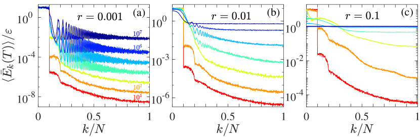
Figure 1: (a)-(c) The function of $\langle\bar{E}_{k}(t)/\varepsilon\rangle$ versus $k/N$ at different time $T$, for the AH chain with different perturbation strength $r$, with ensemble average measurements for $120$ different random choices of the phases, in semilogarithmic scale. In all three panels, the lines from the bottom (red) to top (blue), respectively, correspond to the results of $T=10^{1},10^{2},10^{3},10^{4},10^{5},10^{6},10^{7}$. All numerical results are obtained with the size of system $N=1023$, and energy density $\varepsilon=10^{-3}$. Initial excitation of modes with $0<k/N\leq 0.1$.

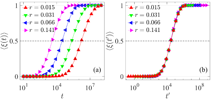
Figure 2: (a) The function of $\langle\xi(t)\rangle$ versus $t$ for the AH chain with different perturbation strength $r$, in semilogarithmic scale. (b) The same as (a) but the curves are shifted properly in the horizontal direction (with that for $r=0.066$ unshifted) so that they perfectly overlap with each other. The size of system $N=2047$, and energy density $\varepsilon=10^{-3}$ are kept fixed. Energy is initially distributed among $10\%$ of modes of the lowest frequencies.

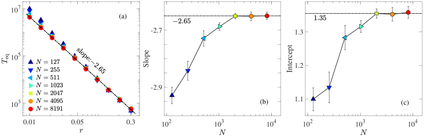
Figure 3: (a) The thermalization time $T_{\rm eq}$ as a function of the perturbation strength $r$ for the AH chain with different sizes of the system in the log-log scale. The dashed line with the slope of $-2.65$ is drawn for reference. Panels (b) and (c) are, respectively, the slope and intercept of the linear fitting of the data of different sizes in panel (a) vary with the size of the chain in semilogarithmic scale. The energy density $\varepsilon=10^{-3}$ is kept fixed. In all simulations, energy is initially distributed among $10\%$ of modes of the lowest frequencies.

To observe the overall process of thermalization dynamics, and obtain the thermalization time $T_{\rm eq}$, we study the evolution of $\langle\xi(t)\rangle$ defined by Eq. (9). Figure 2 shows the numerical results for the AH chain with different $r$. It is seen that on a sufficiently large time scale, all values of $\langle\xi(t)\rangle$ increase from $0$ to $1$ with very similar sigmoidal profiles, which means that the equipartition of energy is finally achieved. Meanwhile, it is also seen that the time required to reach the state of equipartition increases as $r$ decreases. Based on the definition of the equipartition, the thermalization time $T_{\rm eq}$ is defined as that when $\langle\xi(t)\rangle$ reaches the threshold value $1$. However, only the scaling behavior of $T_{\rm eq}$, but not the specific value is usually interested. Thus, we here define the $T_{\rm eq}$ as that when $\langle\xi(t)\rangle$ arrives at the threshold value $0.5$ to save the cost of calculation. This is very artificial; however, it does not influence the scaling behavior of $T_{\rm eq}$ Gallavotti (2008). As can be seen from Fig. 2(b) that the sigmoidal profiles in Fig. 2(a) can completely overlap with each other upon suitable shifts, which suggests that the concrete threshold value does not affect the scaling law of $T_{\rm eq}$. In the following, we will study the dependencies of the $T_{\rm eq}$ on $r$, $N$ for the AH chain, and $r$, $\beta$ for the AH-$\beta$ one.

In Fig. 3(a), we present the dependence of $T_{\rm eq}$ on $r$ in the log-log scale, for the AH chain with different values of $N$ at the fixed energy density $\varepsilon=10^{-3}$. In the explored range of $r$, $T_{\rm eq}$ becomes nearly independent of $N$ with the further increase of $N$. The numerical results show that $N=2047$ seems large enough that the thermodynamic limit is practically achieved. It is seen that $T_{\rm eq}$ versus $r$ exhibits a power-law behavior,

$$T_{\rm eq}\propto r^{\lambda}.$$ (13)

Figure 3(b) and 3(c) show, respectively, the dependence of the slope $\lambda$ and the intercept of the linear fitting of the data in Fig. 3(a) on $N$, in the semilogarithmic scale. It can be seen that the $\lambda$ rapidly saturates at $-2.65$, while the intercept saturates at $1.35$. Then we can give a rough estimate of the $T_{\rm eq}$ for the AH model in the thermodynamic limit,

$$T_{\rm eq}^{\text{AH}}\simeq 10^{1.35}r^{-2.65}\simeq 22.39r^{-2.65},$$ (14)

which deviates from the previously found inverse square law Fu et al. (2019a, b); Pistone et al. (2019); Fu et al. (2019c); Wang et al. (2020a, b); Fu et al. (2021). This phenomenon of the steeper slope is also observed in the model with the odd-order nonlinearity (e.g., the FPUT-$\alpha$ chain) Fu et al. (2019b); Pistone et al. (2019). Yet, the mechanism of this deviation is still unclear. In Ref. Pistone et al. (2019), it is suggested that the deviation is caused by the finite-size effect (discreteness), while in Ref. Fu et al. (2019b), it is shown that the results of different system size almost coincide in the range of studied parameters, but the steeper slope is still observed; in addition, it has been pointed out that the asymmetric IIP will lead to the asymmetric spectral peaks of modes (i.e., the higher-order effect), which is considered as the root of the deviation. The AH model, as a pure asymmetric one without nonlinearity, still shows the deviation, which further demonstrates that the asymmetry results in the steeper slope. Next, we will detect the role of the nonlinearity, which is exemplified by the AH-$\beta$ model [see again Eq. (3)].

Figure 4 shows the dependence of $T_{\rm eq}$ on $r$ in the log-log scale for the AH-$\beta$ chain with different values of $\beta$ at the fixed $N=8191$. It can be seen that the $T_{\rm eq}$ of the chain tends to saturation values with the decrease of $r$, and the saturation values decrease with the increase of $\beta$, which illustrates that the thermalization behavior of the AH-$\beta$ model is dominated by the fourth-order nonlinearity in the case of small $r$, while the thermalization behavior of the system is completely dominated by the asymmetry with the increase of $r$. This result further shows that there is a competitive relationship between the asymmetry and the fourth-order nonlinearity in the thermalization process. If the effects of these two factors on thermalization are independent of each other, as Ref. Fu et al. (2019b) suggested, then we can apply Matthiessen’s rule (MR) Srivastava (1990) to integrate their contributions. Thus, for the AH-$\beta$ chain, it is estimated that $T_{\rm eq}$ follows

$$\frac{1}{T_{\rm eq}^{\text{AH-}\beta}}=\frac{1}{T_{\rm eq}^{\text{AH}}}+\frac{1}{T_{\rm eq}^{\text{FPUT-}\beta}},$$ (15)

where $T_{\rm eq}^{\text{AH}}$ has been given by Eq. (14). While $T_{\rm eq}^{\text{FPUT-}\beta}\propto\beta^{-2}$ in the thermodynamic limit Fu et al. (2019b); Pistone et al. (2019), the thermalization time taken from Ref. Fu et al. (2019b), gives a rough estimate of the $T_{\rm eq}$ for the FPUT-$\beta$ chain,

$$T_{\rm eq}^{\text{FPUT-}\beta}\simeq 3\beta^{-2}.$$ (16)

Combined with Eqs. (14), (15), and (16), we thus can give a specific estimate of the $T_{\rm eq}$ for the AH-$\beta$ chain as

$$T_{\rm eq}^{\text{AH-}\beta}=\frac{67.17r^{-2.65}\beta^{-2}}{22.39r^{-2.65}+3\beta^{-2}}.$$ (17)

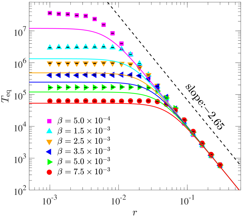
Figure 4: The thermalization time $T_{\rm eq}$ as a function of the perturbation strength $r$ for the AH-$\beta$ chain with different strength of nonlinearity $\beta$ at the fixed system size $N=8191$. The solid curves are estimations given by Eq. (17). The dashed line with slope $-2.65$ is drawn for reference. Initial excitation of modes with $0<k/N\leq 0.1$.

The solid lines in Fig. 4 are function curves of Eq. (17). It can be seen that the trend of the function curves and that of the numerical results are the same, but with the decrease of $\beta$, the deviation between the function curves and the numerical results becomes larger and larger, which is led by the finite-size effect. For example, in Refs. Lvov and Onorato (2018); Onorato et al. (2015), it has been pointed out that the timescale of the resonant four-wave kinetic equation is given by the $\beta^{-2}$, however, the exact four-wave resonances exist only when the size of chain $N\geq 163264$ Onorato et al. (2015); Nazarenko (2011). Nevertheless, because of the nonlinearity, each mode corresponds to a spectral peak of a nonzero width, which will result in the four-wave near-resonance interaction occurring Gershgorin et al. (2005). And the stronger the nonlinearity is, the easier the near-resonance interaction happens. In short, to see $T_{\rm eq}\propto\beta^{-2}$ requires a larger size at extremely weak nonlinearity, or, a stronger nonlinearity at a relatively limited size Fu et al. (2019b). This is why the deviation occurs in the range of small $\beta$, but nearly vanishes when $\beta$ becomes larger. In addition, from Eq. (17), it can be easily proved that $\partial T_{\rm eq}/\partial r<0$, namely, $T_{\rm eq}$ will decrease monotonically with the increase of $r$ for a given $\beta$. Similarly, $\partial T_{\rm eq}/\partial\beta<0$ also holds, which means that for a given $r$, $T_{\rm eq}$ will decrease monotonically as $\beta$ increases. Yet, this is not the case.

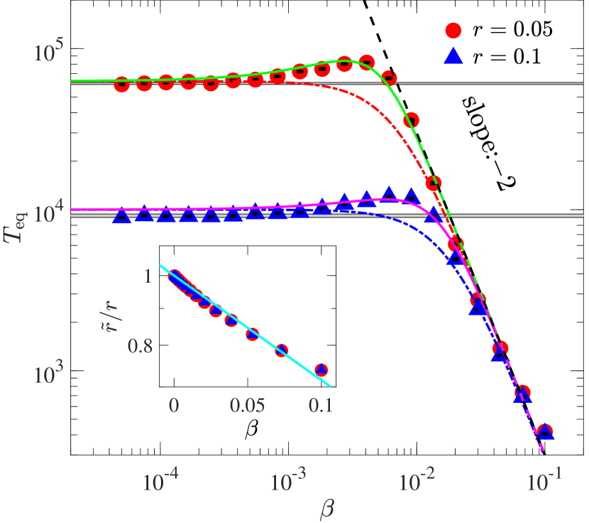
Figure 5: The thermalization time $T_{\rm eq}$ as a function of the strength of nonlinearity $\beta$ for the AH-$\beta$ chain with fixed perturbation strength $r=0.05$ (red circles), and $r=0.1$ (blue up-triangles). The dashed-dotted curves are estimations given by Eq. (17). The solid lines are fitting curves based on Eq. (18). The dashed line given by Eq. (16) is drawn for reference. Fitting parameter: $\gamma=72.21$ for $r=0.05$; and $\gamma=18.58$ for $r=0.1$. The horizontal gray area corresponds to $T_{\rm eq}$ of the AH model (i.e., AH-$\beta$ model with $\beta=0$), and the width represents the range of error. In all simulations, the size of system $N=2047$ is fixed. Initial excitation of modes with $0<k/N\leq 0.1$. Inset: The normalized effective degree of asymmetry $\tilde{r}/r$ as a function of nonlinearity strength $\beta$ in semilogarithmic scale with the vertical axis the logarithmic. The corresponding parameters of the circles and up-triangles are the same as those in the main panel. The solid line with the function of $e^{-3.35\beta}$ is drawn for reference.

Figure 5 presents the thermalization time $T_{\rm eq}$ as a function of $\beta$ in the log-log scale for the AH-$\beta$ chain with $r=0.05$ (red circles) and $r=0.1$ (blue up-triangles) at the fixed $N=2047$. The dashed-dotted curves are estimations of $T_{\rm eq}$ given by the Eq. (17). It is noted that the overall trend of the dashed-dotted lines and that of the data points are in good agreement, but it is also recognized that there are significant qualitative differences when $\beta$ is in the middle range, which shows that the $T_{\rm eq}$ varies non-monotonically as $\beta$ increases. Namely, after introducing nonlinearity into the AH model, the $T_{\rm eq}$ of the system increases firstly, then decreases, with continuous enhancement of the nonlinearity. This phenomenon is somewhat counterintuitive because the general view is that the enhancement of nonlinearity will promote the thermalization of the system.

How to understand the deviation between the numerical results and the MR’s estimation? In fact, according to the theory of condensed matter physics, the MR works only if the multiple scattering processes are independent of each other. While an intuitive physical picture is that the effective asymmetry of IIP decreases gradually with the increase of the fourth-order nonlinearity for a given $r$. An extreme example is that when $\beta$ tends to be infinity, the interaction potential becomes a completely symmetric one, which means that the effective degree of asymmetry $\tilde{r}$ approaches zero Fu and Zhao (2015). The method presented in Ref. Fu and Zhao (2015) is adopted to calculate the effective degree of asymmetry for the AH-$\beta$ model and the results are shown in the inset of Fig. 5. It is shown that with the increase of $\beta$, the effective degree of asymmetry $\tilde{r}$ approximately decays exponentially. Here we consider this effect and assume that $\tilde{r}=re^{-\gamma\beta}$, where $\gamma$ is an undetermined parameter. Given this, Eq. (17) can be modified as

$$T_{\rm eq}^{\text{AH-}\beta}=\frac{67.17(re^{-\gamma\beta})^{-2.65}\beta^{-2}}{22.39(re^{-\gamma\beta})^{-2.65}+3\beta^{-2}}.$$ (18)

The solid lines in Fig. 5 are fitting curves based on Eq. (18). It can be seen that the solid curve covers almost all data points. It should be pointed out that the fitting parameter $\gamma$ is different from the one obtained from the calculation presented in the inset. Except for differences in values, the former is highly dependent on $r$ while the latter is not. The differences may come from the two approximations: one is the exponential form itself; the other is the independence of the effective degree of asymmetry and the nonlinearity strength in the application of MR. While the specific reason for the differences is still an open question that needs to be further studied. Anyway, the consistency between the fitting curves and the numerical results shows that the above considerations of correction are reasonable to a certain extent. In short, for a given $r$, the enhancement of symmetric nonlinearity will rapidly reduce the effective degree of asymmetry of the IIP, then the counterintuitive result appears, i.e., $T_{\rm eq}$ varies non-monotonically with $\beta$. In fact, for a given $\beta$, the strength of nonlinearity also varies with the change of the degree of asymmetry, since the variation of the latter will lead to the change of the distribution function of the relative displacement, and then the proportion of the nonlinear energy in the total. However, the numerical results here show that this effect is very weak, as shown in Fig. 4 that the simulation results agree well with the MR’s estimation.

IV Summary And Discussions

In summary, we have studied the thermalization behavior of a 1D lattice chain, in which the particles are in a purely asymmetric interaction potential without nonlinearity, which is named as the AH model to study the effect of the asymmetry of the IIP on thermalization. Our numerical results show that, in the AH model, there is no metastable state similar to that observed in the perturbed Toda one (see again Fig. 1), since the non-smoothness of the IIP at $x=0$ destroys the Toda integrability. Thus, the AH model should be regarded as the perturbation of the harmonic chain, and the degree of asymmetry is the perturbation strength. Then, it is shown that, in the thermodynamic limit, the relationship between the thermalization time and the perturbation strength still satisfies a power-law, with the exponent of which however larger than that of the previously found universal scaling law (see again Fig. 3). The results are qualitatively consistent with those of the cubic nonlinear (FPUT-$\alpha$) chain Fu et al. (2019b); Pistone et al. (2019) and the quintic nonlinear one Fu et al. (2019b). In Ref. Pistone et al. (2019), the steeper slope is speculated to be caused by the finite-size effect (discreteness). However, the numerical results presented here and in Ref. Fu et al. (2019b) show that the finite-size effect of the models of asymmetric IIP is very weak, and the results converge rapidly with the increase of the system size. Therefore, the higher-order effect caused by the asymmetry may be the source of the steeper slope. One more thing that is worth noting for the AH model is that it can avoid the phenomenon of blowup in simulations of the odd-order nonlinear models as mentioned in Refs. Pistone et al. (2019); Carati and Ponno (2018), and this model can thus be used to study the higher-order effect. Of course, how asymmetry leads to the stronger higher-order effect and the steeper slope are interesting problems that need to be further clarified.

Moreover, the thermalization behavior under the case where the asymmetry and nonlinearity are interwoven (i.e., the AH-$\beta$ model) is also considered. It is found that the $T_{\rm eq}$ of the AH-$\beta$ chain can be described by the MR. And it is obvious that when the quartic nonlinearity is large enough and dominant, the previously found inverse square law of thermalization reappears. Another thing worth noting is the qualitative deviation between the data points and the uncorrected prediction of the MR (see again Fig. 5). It is due to the interrelationship between the asymmetry and the nonlinearity. In fact, coexisting multi-factors usually have complicated interactions where complex phenomena often live in. Therefore, it is necessary to explore the effect of each of the multi-factors separately, and the clear paradigm provided here may be a choice.

References

- Fermi et al. (1955) E. Fermi, J. Pasta, and S. Ulam, Los Alamos Scientific Laboratory, Report No. LA-1940 (1955).
- Cha (2005) Chaos focus issue: The “Fermi-Pasta-Ulam” problem—the first 50 years, Chaos 15 (2005).
- Gallavotti (2008) G. Gallavotti, ed., The Fermi-Pasta-Ulam Problem: A Status Report, Lect. Notes Phys., Vol. 728 (Springer, New York, 2008).
- Ferguson et al. (1982) W. Ferguson, H. Flaschka, and D. McLaughlin, J. Computat. Phys. 45, 157 (1982).
- Casetti et al. (1997) L. Casetti, M. Cerruti-Sola, M. Pettini, and E. G. D. Cohen, Phys. Rev. E 55, 6566 (1997).
- Ponno et al. (2011) A. Ponno, H. Christodoulidi, C. Skokos, and S. Flach, Chaos 21, 043127 (2011).
- Benettin et al. (2013) G. Benettin, H. Christodoulidi, and A. Ponno, J. Stat. Phys. 152, 195 (2013).
- Benettin et al. (2018) G. Benettin, S. Pasquali, and A. Ponno, J. Stat. Phys. 171, 521 (2018).
- Goldfriend and Kurchan (2019) T. Goldfriend and J. Kurchan, Phys. Rev. E 99, 022146 (2019).
- Grava et al. (2020) T. Grava, A. Maspero, G. Mazzuca, and A. Ponno, Commun. Math. Phys. 380, 811 (2020).
- Benettin and Ponno (2020) G. Benettin and A. Ponno, Math. Eng. 3, 1 (2020).
- Onorato et al. (2015) M. Onorato, L. Vozella, D. Proment, and Y. V. Lvov, Proc. Natl. Acad. Sci. 112, 4208 (2015).
- Lvov and Onorato (2018) Y. V. Lvov and M. Onorato, Phys. Rev. Lett. 120, 144301 (2018).
- Pistone et al. (2018) L. Pistone, M. Onorato, and S. Chibbaro, EPL (Europhysics Letters) 121, 44003 (2018).
- Fu et al. (2019a) W. Fu, Y. Zhang, and H. Zhao, New J. Phys. 21, 043009 (2019a).
- Fu et al. (2019b) W. Fu, Y. Zhang, and H. Zhao, Phys. Rev. E 100, 010101(R) (2019b).
- Pistone et al. (2019) L. Pistone, S. Chibbaro, M. Bustamante, Y. L’vov, and M. Onorato, Math. Eng. 1, 672 (2019).
- Fu et al. (2019c) W. Fu, Y. Zhang, and H. Zhao, Phys. Rev. E 100, 052102 (2019c).
- Wang et al. (2020a) Z. Wang, W. Fu, Y. Zhang, and H. Zhao, Phys. Rev. Lett. 124, 186401 (2020a).
- Wang et al. (2020b) Z. Wang, W. Fu, Y. Zhang, and H. Zhao, “Universal time scale for thermalization in two-dimensional systems,” (2020b), arXiv:2005.03478 [cond-mat.stat-mech] .
- Fu et al. (2021) W. Fu, Y. Zhang, and H. Zhao, Phys. Rev. E 104, L032104 (2021).
- Kittel et al. (1996) C. Kittel, P. McEuen, and P. McEuen, Introduction to solid state physics, Vol. 8 (Wiley New York, 1996).
- Lepri (2016) S. Lepri, ed., Thermal Transport in Low Dimensions: From Statistical Physics to Nanoscale Heat Transfer, Lect. Notes Phys., Vol. 921 (Springer, New York, 2016).
- Lee-Dadswell et al. (2005) G. R. Lee-Dadswell, B. G. Nickel, and C. G. Gray, Phys. Rev. E 72, 031202 (2005).
- Lee-Dadswell et al. (2008) G. Lee-Dadswell, B. Nickel, and C. Gray, J. Stat. Phys. 132, 1 (2008).
- Delfini et al. (2006) L. Delfini, S. Lepri, R. Livi, and A. Politi, Phys. Rev. E 73, 060201(R) (2006).
- Delfini et al. (2007) L. Delfini, S. Lepri, R. Livi, and A. Politi, J. Stat. Mech.: Theory Exp. 2007, P02007 (2007).
- van Beijeren (2012) H. van Beijeren, Phys. Rev. Lett. 108, 180601 (2012).
- Spohn (2014) H. Spohn, J. Stat. Phys. 154, 1191 (2014).
- Zhong et al. (2012) Y. Zhong, Y. Zhang, J. Wang, and H. Zhao, Phys. Rev. E 85, 060102(R) (2012).
- Zhong et al. (2013) Y. Zhong, Y. Zhang, J. Wang, and H. Zhao, Chin. Phys. B 22, 070505 (2013).
- Chen et al. (2016) S. Chen, Y. Zhang, J. Wang, and H. Zhao, J. Stat. Mech.: Theory Exp. 2016, 033205 (2016).
- Jiang and Zhao (2016) J. Jiang and H. Zhao, J. Stat. Mech. Theory Exp. 2016, 093208 (2016).
- Wang et al. (2013) L. Wang, B. Hu, and B. Li, Phys. Rev. E 88, 052112 (2013).
- Das et al. (2014) S. G. Das, A. Dhar, and O. Narayan, J. Stat. Phys. 154, 204 (2014).
- Chen et al. (2014) S. Chen, J. Wang, G. Casati, and G. Benenti, Phys. Rev. E 90, 032134 (2014).
- Zhao and Wang (2018) H. Zhao and W. g. Wang, Phys. Rev. E 97, 010103(R) (2018).
- Lepri et al. (2020) S. Lepri, R. Livi, and A. Politi, Phys. Rev. Lett. 125, 040604 (2020).
- Campbell et al. (2004) D. K. Campbell, S. Flach, and Y. S. Kivshar, Phys. Today 57, 43 (2004).
- Benettin and Ponno (2011) G. Benettin and A. Ponno, J. Stat. Phys. 144, 793 (2011).
- Livi et al. (1985) R. Livi, M. Pettini, S. Ruffo, M. Sparpaglione, and A. Vulpiani, Phys. Rev. A 31, 1039 (1985).
- Yoshida (1990) H. Yoshida, Phys. Lett. A 150, 262 (1990).
- Benettin et al. (2009) G. Benettin, R. Livi, and A. Ponno, J. Stat. Phys. 135, 873 (2009).
- Srivastava (1990) G. P. Srivastava, The physics of phonons (Hilger, Bristol, 1990).
- Nazarenko (2011) S. Nazarenko, ed., Wave Turbulence, Lecture Notes in Physics, Berlin Springer Verlag, Vol. 825 (2011).
- Gershgorin et al. (2005) B. Gershgorin, Y. V. Lvov, and D. Cai, Phys. Rev. Lett. 95, 264302 (2005).
- Fu and Zhao (2015) W. Fu and H. Zhao, “Effective phonon treatment of asymmetric interparticle interaction potentials,” (2015), arXiv:1511.00551 [cond-mat.stat-mech] .
- Carati and Ponno (2018) A. Carati and A. Ponno, J. Stat. Phys. 170, 883 (2018).