Nonlinear Deterministic Filter for Inertial Navigation and Bias Estimation with Guaranteed Performance

Abstract

Unmanned vehicle navigation concerns estimating attitude, position, and linear velocity of the vehicle the six degrees of freedom (6 DoF). It has been known that the true navigation dynamics are highly nonlinear modeled on the Lie Group of $\mathbb{SE}_{2}(3)$. In this paper, a nonlinear filter for inertial navigation is proposed. The filter ensures systematic convergence of the error components starting from almost any initial condition. Also, the errors converge asymptotically to the origin. Experimental results validates the robustness of the proposed filter.

I Introduction

Navigation solutions are key element in autonomous vehicles [1, 2]. Navigation estimation algorithms considers the vehicle orientation (attitude), position, and linear velocity to be completely unknown and require estimating the aforementioned three elements[3, 4]. Navigation solutions become indispensable if global positioning systems (GPS) are unreliable. A set of measurements is required for the estimation process. The vehicle’s orientation can be estimated using for instance, inertial measurement unit (IMU) [5, 6, 7, 8, 9], while vehicle’s pose (orientation and position) can be estimated using IMU and vision unit [10]. Recently, other potential solutions emerged to estimate the vehicle’s pose as well as map the unknown environment such as nonlinear deterministic filter for simultaneous localization and mapping (SLAM) [11, 12] and nonlinear stochastic filter for SLAM [1]. The family of pose and SLAM filters requires linear velocity to be known. In practice, linear velocity is hard to obtain in GPS-denied regions and it is challenging to reconstruct.

Traditionally, inertial navigation used to addressed using Gaussian filters, such as Kalman filter [13], extended Kalman filter [14], unscented Kalman filter [15], and particle filter which is non-Gaussian filter [16] among others. Gaussian filters are based on linear approximation while particle filters do not have clear measure for optimal performance. However, navigation dynamics of a vehicle navigating in three dimensional (3D) space are highly nonlinear. Also, the dynamics cannot be classified as right or left invariant. Thereby, a recent development of filters for inertial navigation on the Lie Group have been developed, for instance invariant extended Kalman filter (IEKF) on the Lie Group of $\mathbb{SE}_{2}(3)$ [17], a Riccati filter design [18], and a nonlinear stochastic filter on the Lie group of $\mathbb{SE}_{2}(3)=\mathbb{SO}\left(3\right)\times\mathbb{R}^{3}\times\mathbb{R}^{3}\subset\mathbb{R}^{5\times 5}$ [3, 4]. The filters in [17, 18, 3, 4] are developed directly on $\mathbb{SE}_{2}(3)$, however measures of transient and steady-state can be defined.

To sum up, the navigation dynamics are highly nonlinear posed on the Lie group of $\mathbb{SE}_{2}(3)$. Also, the transient and steady-state error has to be taken into account. It is worth noting that navigation filters relies on gyroscope and accelerometer measurements, and therefore, uncertainties in gyroscope and accelerometer measurements should be addressed. Hence, this paper consider the previously mentioned challenges through the following set of contributions: (1) A nonlinear filter on the Lie Group of $\mathbb{SE}_{2}(3)$ for inertial navigation with predefined measures of transient and steady-state performance is proposed; (2) the closed loop errors are shown to be almost globally asymptotically stable, and when provided with data from low-cost IMU and feature sensors; and (3) the presence of unknown bias in IMU measurements is successfully tackled.

The rest of the paper is organized as follows: Section II presents important notation and identities, and introduces the true navigation problem. Section III present the concept of guaranteed measures of transient and steady-state performance and proposes a novel nonlinear filter. Section IV shows experimental results. Finally, Section V concludes the work.

II Navigation Framework

II-A Preliminaries

Let $\mathbb{R}$ set of real numbers, and $\mathbb{R}^{n\times m}$ denote denote an $n$-by-$m$ real real numbers. $\mathbf{I}_{n}$ is an $n$-by-$n$ identity matrix and $0_{n\times m}$ is an $n$-by-$m$ dimensional matrix of zeros. $\left\{\mathcal{I}\right\}$ stands for the fixed inertial-frame and $\left\{\mathcal{B}\right\}$ corresponds to the fixed body-frame attached to a vehicle moving in 3D space. The vehicle’s orientation in 3D space, known as attitude, is described by $R\in\mathbb{SO}\left(3\right)$ where $\mathbb{SO}\left(3\right)$ is a short-hand notation for Special Orthogonal Group given by

$$\mathbb{SO}\left(3\right)=\left\{\left.R\in\mathbb{R}^{3\times 3}\right|RR^{\top}=R^{\top}R=\mathbf{I}_{3}\text{, }{\rm det}\left(R\right)=+1\right\}$$

where ${\rm det}\left(\cdot\right)$ stands for a determinant. $\mathfrak{so}\left(3\right)$ is the Lie-algebra of $\mathbb{SO}\left(3\right)$ denoted by

$$\mathfrak{so}\left(3\right) =\left\{\left.\left[x\right]_{\times}\in\mathbb{R}^{3\times 3}\right|\left[x\right]_{\times}^{\top}=-\left[x\right]_{\times},x\in\mathbb{R}^{3}\right\}$$

$$\left[x\right]_{\times}=\left[\begin{array}[]{ccc}0&-x_{3}&x_{2}\\ x_{3}&0&-x_{1}\\ -x_{2}&x_{1}&0\end{array}\right]\in\mathfrak{so}\left(3\right),\hskip 10.00002ptx=\left[\begin{array}[]{c}x_{1}\\ x_{2}\\ x_{3}\end{array}\right]$$

The following mappings are defined

$$\mathbf{vex}([x]_{\times}) =x,\hskip 10.00002pt\forall x\in\mathbb{R}^{3}$$ (1)

$$\boldsymbol{\mathcal{P}}_{a}(M) =\frac{1}{2}(M-M^{\top})\in\mathfrak{so}\left(3\right),\hskip 10.00002pt\forall M\in\mathbb{R}^{3\times 3}$$ (2)

$$\boldsymbol{\Upsilon}\left(M\right) =\mathbf{vex}(\boldsymbol{\mathcal{P}}_{a}(M))\in\mathbb{R}^{3},\hskip 10.00002pt\forall M\in\mathbb{R}^{3\times 3}$$ (3)

Define $||R||_{{\rm I}}$ as the Euclidean distance of $R\in\mathbb{SO}\left(3\right)$ such that

$$||R||_{{\rm I}}=\frac{1}{4}{\rm Tr}\{\mathbf{I}_{3}-R\}\in\left[0,1\right]$$ (4)

For more information about attitude and pose notation visit [5, 10]. The extended form of the Special Euclidean Group denoted by $\mathbb{SE}_{2}\left(3\right)=\mathbb{SO}\left(3\right)\times\mathbb{R}^{3}\times\mathbb{R}^{3}\subset\mathbb{R}^{5\times 5}$ is defined by

$$\mathbb{SE}_{2}\left(3\right)= \{\left.X\in\mathbb{R}^{5\times 5}\right|R\in\mathbb{SO}\left(3\right),P,V\in\mathbb{R}^{3}\}$$ (5)

$$X= \left[\begin{array}[]{ccc}R&P&V\\ 0_{1\times 3}&1&0\\ 0_{1\times 3}&0&1\end{array}\right]\in\mathbb{SE}_{2}\left(3\right)$$ (9)

where $X$, $R$, $P$, and $V$ denote a homogeneous navigation matrix, rigid-body’s orientation, position, and linear velocity, respectively, Let $\mathcal{U}_{\mathcal{M}}=\mathfrak{so}\left(3\right)\times\mathbb{R}^{3}\times\mathbb{R}^{3}\times\mathbb{R}$ be a submanifold of $\mathbb{R}^{5\times 5}$ where

$$\mathcal{U}_{\mathcal{M}} =\left\{\left.u\left(\text{$\left[\Omega\right]_{\times}$},V,a,\kappa\right)\right|\text{$\left[\Omega\right]_{\times}$}\in\mathfrak{so}\left(3\right),V,a\in\mathbb{R}^{3},\kappa\in\mathbb{R}\right\}$$

$$u\left(\text{$\left[\Omega\right]_{\times}$},V,a,\kappa\right)=\left[\begin{array}[]{ccc}\left[\Omega\right]_{\times}&V&a\\ 0_{1\times 3}&0&0\\ 0_{1\times 3}&\kappa&0\end{array}\right]\in\mathcal{U}_{\mathcal{M}}$$ (13)

with $\Omega\in\mathbb{R}^{3}$ and $a\in\mathbb{R}^{3}$ being the vehicle’s true angular velocity and the apparent acceleration composed of all non-gravitational forces affecting the vehicle. It should be remarked that $R,\Omega,a\in\left\{\mathcal{B}\right\}$ and $P,V\in\left\{\mathcal{I}\right\}$.

II-B Navigation Dynamics and Measurements

The true 3D navigation dynamics are highly nonlinear described by [3, 4]

$$\begin{cases}\dot{R}&=R\left[\Omega\right]_{\times}\\ \dot{P}&=V\\ \dot{V}&=Ra+\overrightarrow{\mathtt{g}}\end{cases},\hskip 10.00002pt\underbrace{\dot{X}=XU-\mathcal{\mathcal{G}}X}_{\text{Compact form}}$$ (14)

with the left portion of (14) being the detailed navigation dynamics and the notation were defined in (9) and (13). Also, $\overrightarrow{\mathtt{g}}$ refers to a gravity vector. Note that $\dot{X}:\mathbb{SE}_{2}\left(3\right)\times\mathbb{R}^{3}\times\mathbb{R}^{3}\rightarrow T_{X}\mathbb{SE}_{2}\left(3\right)$ [3, 4]. The right portion of (14) describes the compact form $\dot{X}:\mathbb{SE}_{2}\left(3\right)\times\mathcal{U}_{\mathcal{M}}\rightarrow T_{X}\mathbb{SE}_{2}\left(3\right)$ with $U=\underbrace{\left[\begin{array}[]{ccc}\left[\Omega\right]_{\times}&0_{3\times 1}&a\\ 0_{1\times 3}&0&0\\ 0_{1\times 3}&1&0\end{array}\right]}_{u(\text{$\left[\Omega\right]_{\times}$},0_{3\times 1},a,1)}$, $\mathcal{\mathcal{G}}=\underbrace{\left[\begin{array}[]{ccc}0_{3\times 3}&0_{3\times 1}&-\overrightarrow{\mathtt{g}}\\ 0_{1\times 3}&0&0\\ 0_{1\times 3}&1&0\end{array}\right]}_{u(0_{3\times 3},0_{3\times 1},-\overrightarrow{\mathtt{g}},1)}$ [3, 4]. The measurements of $\Omega$ and $a$ follows:

$$\begin{cases}\Omega_{m}&=\Omega+b_{\Omega}\in\mathbb{R}^{3}\\ a_{m}&=a+b_{a}\in\mathbb{R}^{3}\end{cases}$$ (15)

where $b_{\Omega}$ and $b_{a}$ denote unknown bias. Consider $n$ features in the environment where $p_{i}\in\mathbb{R}^{3}$ denotes the $i$th feature position $p_{i}\in\left\{\mathcal{I}\right\}$ for all $i=1,2,\ldots,n$. Let the $i$th feature measurement be

$$y_{i}=R^{\top}(p_{i}-P)+b_{i}^{y}+n_{i}^{y}\in\mathbb{R}^{3}$$ (16)

whee $b_{i}^{y}$ is an unknown bias and $n_{i}^{y}$ is noise.

Assumption 1

At least three non-collinear features available for measurement at each time instant.

II-C Navigation Matrix: Estimate, Error, and Measurements Setup

Let the estimate of the true homogeneous navigation matrix $X\in\mathbb{SE}_{2}\left(3\right)$ defined in (9) be

$$\hat{X}=\left[\begin{array}[]{ccc}\hat{R}&\hat{P}&\hat{V}\\ 0_{1\times 3}&1&0\\ 0_{1\times 3}&0&1\end{array}\right]\in\mathbb{SE}_{2}\left(3\right)$$ (17)

where $\hat{R}\in\mathbb{SO}\left(3\right)$, $\hat{P}\in\mathbb{R}^{3}$, and $\hat{V}\in\mathbb{R}^{3}$ denote estimates of the true orientation, position, and velocity, respectively. Define the error between $X$ and $\hat{X}$ as

$$\tilde{X}=X\hat{X}^{-1} =\left[\begin{array}[]{ccc}\tilde{R}&\tilde{P}&\tilde{V}\\ 0_{1\times 3}&1&0\\ 0_{1\times 3}&0&1\end{array}\right]$$ (21)

where $\tilde{R}=R\hat{R}^{\top}$, $\tilde{P}=P-\tilde{R}\hat{P}$, and $\tilde{V}=V-\tilde{R}\hat{V}$. A set of measurements have to be defined to be subsequently used as part of the filter design, part of the following definitions can be found at [19, 3, 4]. Let us begin by defining the error:

$$\overset{\circ}{\tilde{y}}_{i} =\overline{p}_{i}-\tilde{X}^{-1}\overline{p}_{i}=\overline{p}_{i}-\hat{X}\overline{y}_{i}$$

$$=\left[(p_{i}-\hat{R}y_{i}-\hat{P})^{\top},0,0\right]^{\top}\in\overset{\circ}{\mathcal{M}}$$ (22)

where $\overset{\circ}{\tilde{y}}_{i}=[\tilde{y}_{i}^{\top},0,0]^{\top}\in\overset{\circ}{\mathcal{M}}$, $p_{i}-\hat{R}y_{i}-\hat{P}=\tilde{p}_{i}-\tilde{P}$, $\tilde{p}_{i}=\hat{p}_{i}-\tilde{R}p_{i}$, and $\tilde{P}=P-\tilde{R}\hat{P}$. Define the following components: $s_{T}=\sum_{i=1}^{n}s_{i}$, $p_{c}=\frac{1}{s_{T}}\sum_{i=1}^{n}s_{i}p_{i}$, and $M=\sum_{i=1}^{n}s_{i}(p_{i}-p_{c})(p_{i}-P)^{\top}=\sum_{i=1}^{n}s_{i}p_{i}p_{i}^{\top}-2\sum_{i=1}^{n}s_{i}p_{i}p_{c}^{\top}+s_{T}p_{c}p_{c}^{\top}$ such that

$$M =\sum_{i=1}^{n}s_{i}p_{i}p_{i}^{\top}-s_{T}p_{c}p_{c}^{\top}$$ (23)

where $s_{i}>0$ denotes the sensor confidence level of the $i$th landmark, and $n\geq 3$ as defined in Assumption 1. One finds $\sum_{i=1}^{n}s_{i}(p_{i}-p_{c})y_{i}^{\top}\hat{R}^{\top}=\sum_{i=1}^{n}s_{i}(p_{i}-p_{c})(p_{i}-P)^{\top}\tilde{R}$ which means that

$$\sum_{i=1}^{n}s_{i}\left(p_{i}-p_{c}\right)y_{i}^{\top}\hat{R}^{\top}= M\tilde{R}$$ (24)

Additionally, the following result can be obtained $\sum_{i=1}^{n}s_{i}\tilde{y}_{i}=\sum_{i=1}^{n}s_{i}(p_{i}-\hat{R}y_{i}-\hat{P})=\sum_{i=1}^{n}s_{i}(p_{i}-\tilde{R}^{\top}p_{i})+\sum_{i=1}^{n}s_{i}\tilde{R}^{\top}\tilde{P}$ such that $\sum_{i=1}^{n}s_{i}\tilde{y}_{i}=s_{T}\tilde{R}^{\top}\tilde{P}_{\varepsilon}$ with $\tilde{P}_{\varepsilon}=\tilde{P}-(\mathbf{I}_{3}-\tilde{R})p_{c}$. Note that $\tilde{R}\rightarrow\mathbf{I}_{3}$ indicates that $\tilde{P}_{\varepsilon}\rightarrow\tilde{P}$ and $\tilde{R}=\mathbf{I}_{3}$ implying that $\tilde{R}^{\top}\tilde{P}_{\varepsilon}=\tilde{P}_{\varepsilon}=\tilde{P}$. Summing up the above derivations, the following set expressed in terms of vector measurements will be used in the filter design [3, 4]:

$$\begin{cases}p_{c}&=\frac{1}{s_{T}}\sum_{i=1}^{n}s_{i}p_{i},\hskip 10.00002pts_{T}=\sum_{i=1}^{n}s_{i}\\ M&=\sum_{i=1}^{n}s_{i}p_{i}p_{i}^{\top}-s_{T}p_{c}p_{c}^{\top}\\ \tilde{y}_{i}&=p_{i}-\hat{R}y_{i}-\hat{P}\\ M\tilde{R}&=\sum_{i=1}^{n}s_{i}\left(p_{i}-p_{c}\right)y_{i}^{\top}\hat{R}^{\top}\\ \tilde{R}^{\top}\tilde{P}_{\varepsilon}&=\frac{1}{s_{T}}\sum_{i=1}^{n}s_{i}\tilde{y}_{i}\end{cases}$$ (25)

II-D Nonlinear Filter Framework and Error Dynamics

Lemma 1

Let $\tilde{R}\in\mathbb{SO}\left(3\right)$, $M=M^{\top}\in\mathbb{R}^{3\times 3}$. Define $\overline{\mathbf{M}}={\rm Tr}\{M\}\mathbf{I}_{3}-M$ such that $\underline{\lambda}_{\overline{\mathbf{M}}}=\underline{\lambda}(\overline{\mathbf{M}})$ and $\overline{\lambda}_{\overline{\mathbf{M}}}=\overline{\lambda}(\overline{\mathbf{M}})$ are the minimum and the maximum eigenvalues of $\overline{\mathbf{M}}$, respectively. Then, one has

$$\frac{\underline{\lambda}_{\overline{\mathbf{M}}}}{2}(1+{\rm Tr}\{\tilde{R}\})||M\tilde{R}||_{{\rm I}} \leq||\boldsymbol{\Upsilon}(M\tilde{R})||^{2}\leq 2\overline{\lambda}_{\overline{\mathbf{M}}}||M\tilde{R}||_{{\rm I}}$$ (26)

Proof:

See ([5], Lemma 1).∎

From Lemma 1, define $\overline{\mathbf{M}}={\rm Tr}\{M\}\mathbf{I}_{3}-M$ given that $\lambda(M)=\{\lambda_{1},\lambda_{2},\lambda_{3}\}$ with $\lambda_{3}\geq\lambda_{2}\geq\lambda_{1}$. In view of Assumption (1), at least two of the eigenvalues in the set $\lambda(M)$ are greater than zero and therefore $\lambda(\overline{\mathbf{M}})=\{\lambda_{3}+\lambda_{2},\lambda_{3}+\lambda_{1},\lambda_{2}+\lambda_{1}\}$ see Section 4.2 in [5].

III Nonlinear Navigation Filter Design

III-A Systematic Convergence

Consider the following error in view of the measurements in (25):

$$e=[e_{1},e_{2},e_{3},e_{4}]^{\top}=\left[||M\tilde{R}||_{{\rm I}},\tilde{P}_{\varepsilon}^{\top}\tilde{R}\right]^{\top}\in\mathbb{R}^{4}$$ (27)

Define $\xi_{i}:\mathbb{R}_{+}\to\mathbb{R}_{+}$ as a positive smooth and time-decreasing function [20]:

$$\xi_{i}\left(t\right)=\left(\xi_{i}^{0}-\xi_{i}^{\infty}\right)\exp\left(-\ell_{i}t\right)+\xi_{i}^{\infty},\hskip 10.00002pt\forall i=1,2,\ldots,4$$ (28)

with $\xi_{i}\left(0\right)=\xi_{i}^{0}>0$ being upper bound of the known large set, $\xi_{i}^{\infty}>0$ being upper bound of the small set, and $\ell_{i}>0$ being convergence rate of $\xi_{i}\left(t\right)$ from $\xi_{i}^{0}$ to $\xi_{i}^{\infty}$. Define the error $e_{i}$ as [20]:

$$e_{i}=\xi_{i}\mathcal{N}(E_{i})$$ (29)

where $E_{i}\in\mathbb{R}$ denotes the transformed error which is unconstrained, and $\mathcal{N}(E_{i})$ denotes a smooth function which is differentiable, strictly increasing, and bounded, for more information see [5, 11]. The inverse transformation of (30) is given by

$$E_{i}=\mathcal{N}^{-1}(e_{i}/\xi_{i})$$ (30)

The inverse transformation in (30) is defined by [5, 11, 20]

$$E_{i}= \frac{1}{2}\begin{cases}\text{ln}\frac{\underline{\delta}_{i}+e_{i}/\xi_{i}}{\bar{\delta}_{i}-e_{i}/\xi_{i}},&\bar{\delta}_{i}>\underline{\delta}_{i}\text{ if }e_{i}\left(0\right)\geq 0\\ \text{ln}\frac{\underline{\delta}_{i}+e_{i}/\xi_{i}}{\bar{\delta}_{i}-e_{i}/\xi_{i}},&\underline{\delta}_{i}>\bar{\delta}_{i}\text{ if }e_{i}\left(0\right)<0\end{cases}$$ (31)

Let us define

$$\begin{split}\Delta_{i}&=\frac{1}{2\xi_{i}}\frac{\partial\mathcal{N}^{-1}\left(e_{i}/\xi_{i}\right)}{\partial\left(e_{i}/\xi_{i}\right)}=\frac{1}{2\xi_{i}}\left(\frac{1}{\underline{\delta}_{i}+e_{i}/\xi_{i}}+\frac{1}{\bar{\delta}_{i}-e_{i}/\xi_{i}}\right)\end{split}$$ (32)

Accordingly, the dynamics of $\dot{E}_{i}$ are

$$\dot{E}_{i} =\Delta_{i}\left(\frac{d}{dt}e_{i}-\frac{\dot{\xi}_{i}}{\xi_{i}}e_{i}\right)$$ (33)

Or to put simply

$$\dot{E}=\left[\begin{array}[]{cc}\Delta_{R}&0_{1\times 3}\\ 0_{3\times 1}&\Delta_{P}\end{array}\right]\left(\frac{d}{dt}e-\left[\begin{array}[]{cc}\mu_{R}&0_{1\times 3}\\ 0_{3\times 1}&\mu_{P}\end{array}\right]e\right)$$ (34)

such that $\mu_{R}=\dot{\xi}_{1}/\xi_{1}$, $\mu_{P}={\rm diag}(\dot{\xi}_{2}/\xi_{2},\dot{\xi}_{3}/\xi_{3},\dot{\xi}_{4}/\xi_{4})$, $\Delta_{R}=\Delta_{1}$, and $\Delta_{P}={\rm diag}(\Delta_{2},\Delta_{3},\Delta_{4})$ where $\mu_{R},\Delta_{R}\in\mathbb{R}$ and $\mu_{P},\Delta_{P}\in\mathbb{R}^{3\times 3}$. For more information of orientation, pose, and SLAM filters with prescribed performance visit [5, 11].

III-B Nonlinear Navigation Filter with Bias Compensation

In this Subsection the unknown bias inevitably present in measurements of angular velocity and acceleration is accounted for. From (15), let $\hat{b}_{\Omega}$ and $\hat{b}_{a}$ denote the estimates of $b_{\Omega}$ and $b_{a}$, respectively. Define the bias error as

$$\begin{cases}\tilde{b}_{\Omega}&=b_{\Omega}-\hat{b}_{\Omega}\\ \tilde{b}_{a}&=\hat{b}_{a}-b_{a}\end{cases}$$ (35)

Consider the following nonlinear filter design on the Lie Group of $\mathbb{SE}_{2}\left(3\right)$:

$$\begin{cases}\dot{\hat{R}}&=\hat{R}[\Omega_{m}-\hat{b}_{\Omega}]_{\times}-\left[w_{\Omega}\right]_{\times}\hat{R}\\ \dot{\hat{P}}&=\hat{V}-\left[w_{\Omega}\right]_{\times}\hat{P}-w_{V}\\ \dot{\hat{V}}&=\hat{R}(a_{m}-\hat{b}_{a})-\left[w_{\Omega}\right]_{\times}\hat{V}-w_{a}\end{cases},\hskip 4.5pt\underbrace{\dot{\hat{X}}=\hat{X}U_{m}-W\hat{X}}_{\text{Compact form}}$$ (36)

such that

$$\begin{cases}w_{\Omega}&=-k_{w}(E_{R}\Delta_{R}+1)\boldsymbol{\Upsilon}(M\tilde{R})\\ w_{V}&=\left[p_{c}-\tilde{R}^{\top}\tilde{P}_{\varepsilon}\right]_{\times}w_{\Omega}-\ell_{P}\tilde{R}^{\top}\tilde{P}_{\varepsilon}-k_{v}\Delta_{P}E_{P}\\ w_{a}&=-\overrightarrow{\mathtt{g}}+k_{a}\left(\delta\left[w_{\Omega}\right]_{\times}-\Delta_{P}\right)E_{P}\\ \dot{\hat{b}}_{\Omega}&=-\gamma_{b}(\Delta_{R}E_{R}+1)\hat{R}^{\top}\boldsymbol{\Upsilon}(M\tilde{R})\\ \dot{\hat{b}}_{a}&=-\gamma_{a}\delta\hat{R}^{\top}E_{P}\end{cases}$$ (37)

with $k_{w}$, $k_{v}$, $k_{a}$, $\delta$, $\ell_{P}$, $\gamma_{b}$, and $\gamma_{a}$ being positive constants, $w_{\Omega}$, $w_{V}$, and $w_{a}$ denoting correction factors $\forall$ $w_{\Omega},w_{V},w_{a}\in\mathbb{R}^{3}$, $\boldsymbol{\Upsilon}(M\tilde{R})=\mathbf{vex}(\boldsymbol{\mathcal{P}}_{a}(M\tilde{R}))$, $E_{R}=E_{1}$, and $E_{P}=[E_{2},E_{3},E_{4}]^{\top}$. Also, $U_{m}=u([\Omega_{m}-\hat{b}_{\Omega}\text{$]_{\times}$},0_{3\times 1},a_{m}-\hat{b}_{a},1)\in\mathcal{U}_{\mathcal{M}}$ and $W=u([w_{\Omega}\text{$]_{\times}$},w_{V},w_{a},1)]\in\mathcal{U}_{\mathcal{M}}$.

Theorem 1

Consider the navigation dynamics in (14) coupled with feature measurements (output $\overline{y}_{i}=X^{-1}\overline{p}_{i}$) for all $i=1,2,\ldots,n$, angular velocity measurements ($\Omega_{m}=\Omega+b_{\Omega}$), and acceleration measurements ($a_{m}=a+b_{a}$). Let Assumption 1 hold. Combine the nonlinear filter design in (36) and (37) with the measurements of $\overline{y}_{i}$, $\Omega_{m}$, and $a_{m}$. Let the design parameters $k_{w}$, $k_{v}$, $k_{a}$, $\ell_{P}$, $\gamma_{b}$, $\gamma_{a}$, $\delta$, $\underline{\delta}_{i}=\bar{\delta}_{i}>|e_{i}(0)|$, $\xi_{i}^{0}>|e_{i}(0)|$ and $\xi_{i}^{\infty}$ be selected as positive constants. Define the set

$$\mathcal{S}= \{\left.(E_{R},E_{P},\tilde{V},\tilde{b}_{\Omega},\tilde{b}_{a})\in\mathbb{R}\times\mathbb{R}^{3}\times\mathbb{R}^{3}\times\mathbb{R}^{3}\times\mathbb{R}^{3}\right|$$

$$\hskip 50.00008ptE_{R}=0,E_{P}=\tilde{V}=\tilde{b}_{\Omega}=\tilde{b}_{a}=0_{3\times 1}\}$$ (38)

given that $E_{R},E_{P}\in\mathcal{L}_{\infty}$ and $\tilde{R}(0)$ does not belong to the unattractive set defined in [5]. Then, 1) the errors $E_{R}$, $E_{P}$, $\tilde{V}$, $\tilde{b}_{\Omega}$, and $\tilde{b}_{a}$ converge asymptotically to $\mathcal{S}$ in (38), 2) the trajectory of $\tilde{R}$ converges asymptotically to $\mathbf{I}_{3}$, and 3) the trajectories of $\tilde{P}$ converge asymptotically to the origin.

Proof:

From (14) and (36), the orientation error dynamics are

$$\dot{\tilde{R}} =-\tilde{R}[\hat{R}(\Omega_{m}-\Omega)]_{\times}+\tilde{R}[w_{\Omega}\text{$]_{\times}$}$$ (39)

where $[\hat{R}\Omega]_{\times}=\hat{R}\left[\Omega\right]_{\times}\hat{R}^{\top}$. From (39), (14), and (36), the position error dynamics are

$$\dot{\tilde{P}} =\tilde{V}-\tilde{R}[\hat{P}]_{\times}\hat{R}(\Omega_{m}-\Omega)+\tilde{R}w_{V}$$ (40)

From (39), (14), and (36), the velocity error dynamics are

$$\dot{\tilde{V}} =-R(a_{m}-a)-\tilde{R}[\hat{V}]_{\times}\hat{R}(\Omega_{m}-\Omega)+\overrightarrow{\mathtt{g}}+\tilde{R}w_{a}$$ (41)

Given that $\Omega_{m}=\Omega+b_{\Omega}$ and $a_{m}=a+b_{a}$, one has

$$\begin{cases}\frac{d}{dt}||M\tilde{R}||_{{\rm I}}&=-\frac{1}{2}\boldsymbol{\Upsilon}(M\tilde{R})^{\top}(\hat{R}\tilde{b}_{\Omega}-w_{\Omega})\\ \frac{d}{dt}\tilde{R}^{\top}\tilde{P}_{\varepsilon}&=\tilde{R}^{\top}\tilde{V}-\left[\hat{P}-p_{c}+\tilde{R}^{\top}\tilde{P}_{\varepsilon}\right]_{\times}\hat{R}\tilde{b}_{\Omega}\\ &\hskip 10.00002pt-\left[p_{c}-\tilde{R}^{\top}\tilde{P}_{\varepsilon}\right]_{\times}w_{\Omega}+w_{V}\\ \frac{d}{dt}\tilde{R}^{\top}\tilde{V}&=-\left[\tilde{R}^{\top}V\right]_{\times}\hat{R}\tilde{b}_{\Omega}-\left[w_{\Omega}\right]_{\times}\tilde{R}^{\top}\tilde{V}\\ &\hskip 10.00002pt+\hat{R}\tilde{b}_{a}+\tilde{R}^{\top}\overrightarrow{\mathtt{g}}+w_{a}\end{cases}$$ (42)

From (42) and (34), one obtains

$$\begin{cases}\dot{E}_{R}&=\Delta_{R}\left(\frac{d}{dt}||M\tilde{R}||_{{\rm I}}-\mu_{R}||M\tilde{R}||_{{\rm I}}\right)\\ \dot{E}_{P}&=\Delta_{P}\left(\frac{d}{dt}\tilde{R}^{\top}\tilde{P}_{\varepsilon}-\mu_{P}\tilde{R}^{\top}\tilde{P}_{\varepsilon}\right)\end{cases}$$ (43)

Consider selecting the following Lyapunov function candidate $\mathcal{L}_{T}=\mathcal{L}_{T}(||M\tilde{R}||_{{\rm I}},E_{R},E_{P},\tilde{R}^{\top}\tilde{V},\hat{R}\tilde{b}_{\Omega},\hat{R}\tilde{b}_{a})$

$$\mathcal{L}_{T}=\mathcal{L}_{R}+\mathcal{L}_{PV}$$ (44)

Let $\overline{\lambda}_{\overline{\mathbf{M}}}=\overline{\lambda}(\overline{\mathbf{M}})$. The function $\mathcal{L}_{R}$ is selected as

$$\mathcal{L}_{R} =E_{R}^{2}+\mathcal{L}_{1}$$ (45)

where $\mathcal{L}_{Rb_{\Omega}}=2||M\tilde{R}||_{{\rm I}}+\frac{1}{2\gamma_{b}}||\tilde{b}_{\Omega}||^{2}+\frac{1}{2\overline{\gamma}_{b}\overline{\lambda}_{\overline{\mathbf{M}}}}\boldsymbol{\Upsilon}(M\tilde{R})^{\top}\hat{R}\tilde{b}_{\Omega}$. $\mathcal{L}_{Rb_{\Omega}}$ in (45) follows

$$\varepsilon_{1}^{\top}\underbrace{\left[\begin{array}[]{cc}2&\frac{-1}{4\overline{\gamma}_{b}\overline{\lambda}_{\overline{\mathbf{M}}}}\\ \frac{-1}{4\overline{\gamma}_{b}\overline{\lambda}_{\overline{\mathbf{M}}}}&\frac{1}{2\gamma_{b}}\end{array}\right]}_{\underline{A}_{1}}\varepsilon_{1}\leq\mathcal{L}_{1}\leq\varepsilon_{1}^{\top}\underbrace{\left[\begin{array}[]{cc}2&\frac{1}{4\overline{\gamma}_{b}\overline{\lambda}_{\overline{\mathbf{M}}}}\\ \frac{1}{4\overline{\gamma}_{b}\overline{\lambda}_{\overline{\mathbf{M}}}}&\frac{1}{2\gamma_{b}}\end{array}\right]}_{\overline{A}_{1}}\varepsilon_{1}$$

with $\varepsilon_{1}=\left[\sqrt{||M\tilde{R}||_{{\rm I}}},||\hat{R}\tilde{b}_{\Omega}||\right]^{\top}$ and $\sqrt{2\overline{\lambda}_{\overline{\mathbf{M}}}||\tilde{R}M||_{{\rm I}}}\geq||\boldsymbol{\Upsilon}(M\tilde{R})||$ as defined in (26), Lemma 1. Both $\underline{A}_{1}$ and $\overline{A}_{1}$ become positive given that

$$\frac{1}{\gamma_{b}}>\frac{1}{16\overline{\gamma}_{b}^{2}\overline{\lambda}_{\overline{\mathbf{M}}}^{2}}$$ (46)

Let $\gamma_{b}$ be selected as in (46). Recall (43) and (42). The derivative of (45) is

$$\dot{\mathcal{L}}_{R} \leq-c_{R}(\Delta_{R}^{2}E_{R}^{2}+1)||M\tilde{R}||_{{\rm I}}-c_{b}||\hat{R}\tilde{b}_{\Omega}||^{2}$$

$$+\frac{c_{\Omega}}{\overline{\gamma}_{b}\sqrt{2\overline{\lambda}_{\overline{\mathbf{M}}}}}\sqrt{||M\tilde{R}||_{{\rm I}}}\,||\hat{R}\tilde{b}_{\Omega}||$$

which can be expressed as

$$\dot{\mathcal{L}}_{R}\leq -\varepsilon_{1}^{\top}\underbrace{\left[\begin{array}[]{cc}c_{R}&\frac{c_{\Omega}}{\overline{\gamma}_{b}\sqrt{2\overline{\lambda}_{\overline{\mathbf{M}}}}}\\ \frac{c_{\Omega}}{\overline{\gamma}_{b}\sqrt{2\overline{\lambda}_{\overline{\mathbf{M}}}}}&c_{b}\end{array}\right]}_{A_{2}}\varepsilon_{1}$$ (49)

$$-c_{R}E_{R}^{2}\Delta_{R}^{2}||M\tilde{R}||_{{\rm I}}$$ (50)

where $\varepsilon_{1}=\left[\sqrt{||M\tilde{R}||_{{\rm I}}},||\hat{R}\tilde{b}_{\Omega}||\right]^{\top}$. It can be deduced that $A_{2}$ become positive by selecting $c_{R}c_{b}\geq\frac{c_{\Omega}^{2}}{2\overline{\gamma}_{b}^{2}\overline{\lambda}_{\overline{\mathbf{M}}}}$ such that

$$\overline{\gamma}_{b} \geq\sqrt{\frac{8c_{\Omega}^{2}(1+{\rm Tr}\{\tilde{R}\})+K_{M}}{2\sqrt{3}(k_{w}-1)\underline{\lambda}_{\overline{\mathbf{M}}}\overline{\lambda}_{\overline{\mathbf{M}}}}}$$ (51)

where $K_{M}=(\sqrt{3}\gamma_{b}+(2(k_{w}-1)\overline{\lambda}_{\overline{\mathbf{M}}}-\gamma_{b})k_{w}^{2})\underline{\lambda}_{\overline{\mathbf{M}}}$. Consider selecting $\overline{\gamma}_{b}$ as in (51) and defining $\underline{\lambda}_{A_{2}}=\underline{\lambda}(A_{2})$. Thus, $\dot{\mathcal{L}}_{R}$ in (50) follows the inequality below

$$\dot{\mathcal{L}}_{R}\leq-\underline{\lambda}_{A_{2}}||\varepsilon_{R}||^{2} -c_{R}E_{R}^{2}\Delta_{R}^{2}||M\tilde{R}||_{{\rm I}}$$ (52)

Let us turn our attention to the second portion of the $\mathcal{L}_{T}$ definition in (44). Define the following Lyapunov function candidate:

$$\mathcal{L}_{PV} =\frac{1}{2}||E_{P}||^{2}+\frac{1}{2k_{a}}||\tilde{V}^{\top}\tilde{R}||^{2}+\frac{1}{2\gamma_{a}}\left\|\hat{R}\tilde{b}_{a}\right\|^{2}$$

$$-\delta E_{P}^{\top}\tilde{R}^{\top}\tilde{V}+\delta_{a}\tilde{b}_{a}^{\top}\hat{R}^{\top}\tilde{R}^{\top}\tilde{V}$$ (53)

It is straightforward to show that $\mathcal{L}_{PV}$ in (53) follows

$$\varepsilon_{2}^{\top}\underbrace{\left[\begin{array}[]{ccc}\frac{1}{2}&\frac{-\delta}{2}&0\\ \frac{-\delta}{2}&\frac{1}{2k_{a}}&\frac{-\delta_{a}}{2}\\ 0&\frac{-\delta_{a}}{2}&\frac{1}{2\gamma_{a}}\end{array}\right]}_{\underline{A}_{3}}\varepsilon_{2}\leq\mathcal{L}_{PV}\leq\varepsilon_{2}^{\top}\underbrace{\left[\begin{array}[]{ccc}\frac{1}{2}&\frac{\delta}{2}&0\\ \frac{\delta}{2}&\frac{1}{2k_{a}}&\frac{\delta_{a}}{2}\\ 0&\frac{\delta_{a}}{2}&\frac{1}{2\gamma_{a}}\end{array}\right]}_{\overline{A}_{3}}\varepsilon_{2}$$

with $\varepsilon_{2}=\left[||E_{P}||,||\tilde{V}^{\top}\tilde{R}||,||\hat{R}\tilde{b}_{a}||\right]^{\top}$. It becomes apparent that $\text{$\underline{A}$}_{3}$, $\overline{A}_{3}$, and in turn $\mathcal{L}_{PV}$ can be made positive, if the following holds $\frac{1}{8\gamma_{a}}(\frac{1}{k_{a}}-\delta^{2})-\frac{\delta_{a}^{2}}{8}>0$ which can be enabled by selecting $\delta,\delta_{a},k_{a},\gamma_{a}>0$ and

$$k_{a} <\frac{1}{\delta_{a}^{2}\gamma_{a}+\delta^{2}}$$ (54)

Let $k_{a}$ be selected as in (54). Recall (43) and (42). The time derivative of $\mathcal{L}_{PV}$ in (53) is as follows:

$$\dot{\mathcal{L}}_{PV}\leq -\varepsilon_{PV}^{\top}\underbrace{\left[\begin{array}[]{cc}k_{v}c_{1}-\delta k_{a}c_{2}&\frac{\delta k_{v}c_{4}}{2}\\ \frac{\delta k_{v}c_{4}}{2}&\delta c_{3}\end{array}\right]}_{A_{4}}\varepsilon_{PV}$$ (57)

$$-\delta_{a}||\hat{R}\tilde{b}_{a}||^{2}+(\delta_{a}c_{a}||\hat{R}\tilde{b}_{a}||+c_{b}||\hat{R}\tilde{b}_{\Omega}||)||\tilde{R}^{\top}\tilde{V}||$$

$$+c_{g}(||\tilde{V}||+||E_{P}||+||\hat{R}\tilde{b}_{a}||)||\mathbf{I}_{3}-\tilde{R}||_{F}$$

$$+c_{b}||\hat{R}\tilde{b}_{\Omega}||\,||E_{P}||+\delta_{a}c_{a}||\hat{R}\tilde{b}_{a}||\,||E_{P}||$$ (58)

where $\varepsilon_{PV}=\left[||E_{P}||,||\tilde{V}^{\top}\tilde{R}||\right]^{\top}$. It becomes clear that $A_{4}$ in (58) can be made positive by selecting

$$\frac{1}{\delta}>\frac{k_{v}^{2}c_{4}^{2}+4k_{a}c_{3}c_{2}}{4c_{3}c_{1}k_{v}}$$ (59)

Let $\delta$ be selected as in (59) and define $\underline{\lambda}_{A_{4}}=\underline{\lambda}(A_{4})$. One may rewrite the inequality in (58) as follows:

$$\dot{\mathcal{L}}_{PV}\leq -\left[\begin{array}[]{c}||\varepsilon_{PV}||\\ ||\hat{R}\tilde{b}_{a}||\end{array}\right]^{\top}\underbrace{\left[\begin{array}[]{cc}\underline{\lambda}_{A_{4}}&\frac{\delta_{a}c_{a}}{2}\\ \frac{\delta_{a}c_{a}}{2}&\delta_{a}\end{array}\right]}_{A_{5}}\left[\begin{array}[]{c}||\varepsilon_{PV}||\\ ||\hat{R}\tilde{b}_{a}||\end{array}\right]$$ (66)

$$+c_{g}(||\tilde{V}||+||E_{P}||+||\hat{R}\tilde{b}_{a}||)||\mathbf{I}_{3}-\tilde{R}||_{F}$$

$$+c_{b}||\hat{R}\tilde{b}_{\Omega}||\,||E_{P}||+c_{b}||\hat{R}\tilde{b}_{\Omega}||\,||\tilde{R}^{\top}\tilde{V}||$$ (67)

It can be shown that $A_{5}$ is positive if the following holds:

$$\delta_{a}<\frac{4\underline{\lambda}_{A_{4}}}{c_{a}^{2}}$$ (68)

Consider selecting $\delta_{a}$ as in (68) and defining $\underline{\lambda}_{A_{5}}=\underline{\lambda}(A_{5})$. Define $\varepsilon_{T}=\left[||\varepsilon_{Pb}||,\sqrt{||M\tilde{R}||_{{\rm I}}},||\hat{R}\tilde{b}_{\Omega}||\right]^{\top}$ and let $c_{n}=\max\{4\overline{\lambda}_{M}c_{g},c_{b}\}$. Hence, one obtains

$$\dot{\mathcal{L}}_{T}\leq -\varepsilon_{T}^{\top}\underbrace{\left[\begin{array}[]{cc}\underline{\lambda}_{A_{5}}&\frac{c_{n}}{2}\mathbf{1}_{1\times 2}\\ \frac{c_{n}}{2}\mathbf{1}_{2\times 1}&\underline{\lambda}_{A_{2}}\mathbf{I}_{2}\end{array}\right]}_{A_{T}}\varepsilon_{T}$$ (71)

$$-\frac{\underline{\lambda}_{\overline{\mathbf{M}}}k_{w}E_{R}^{2}\Delta_{R}^{2}}{4(1+{\rm Tr}\{\tilde{R}\})}||M\tilde{R}||_{{\rm I}}$$ (72)

Select the parameters of $A_{2}$ and $A_{5}$ such that $4\underline{\lambda}_{A_{5}}\underline{\lambda}_{A_{2}}>c_{n}^{2}$ guaranteeing the positive definiteness of $A_{T}$. Accordingly, the following result is obtained:

$$\dot{\mathcal{L}}_{T}\leq-\underline{\lambda}(A_{T})\,||\varepsilon_{T}||^{2}-\frac{\underline{\lambda}_{\overline{\mathbf{M}}}k_{w}E_{R}^{2}\Delta_{R}^{2}}{4(1+{\rm Tr}\{\tilde{R}\})}||M\tilde{R}||_{{\rm I}}$$ (73)

Recall that $\varepsilon_{T}=\left[||\varepsilon_{Pb}||,\sqrt{||M\tilde{R}||_{{\rm I}}},||\hat{R}\tilde{b}_{\Omega}||\right]$ where $\varepsilon_{Pb}=\left[||\varepsilon_{PV}||,||\hat{R}\tilde{b}_{a}||\right]^{\top}$, and $\varepsilon_{PV}=\left[||E_{P}||,||\tilde{V}^{\top}\tilde{R}||\right]^{\top}$. In accordance with the definition of $\mathcal{L}_{T}$ in (44), the inequality in (73) indicates that $\dot{\mathcal{L}}_{T}$ is negative for all $\mathcal{L}_{T}>0$, and $\dot{\mathcal{L}}_{T}=0$ only at $\mathcal{L}_{T}=0$. This ensures asymptotic convergence of $\mathcal{L}_{T}$ enabling the guaranteed performance of transient and steady-state error in (27). This completes the proof.∎

For implementation purposes, the nonlinear navigation filter with guaranteed performance for unknown bias outlined in (36) and detailed in (37) is presented in discrete form. Let $\Delta t$ denote a small sample time step. The complete discrete implementation steps are detailed in Algorithm 1.

Algorithm 1 Discrete nonlinear filter.

Initialization:

1. Set $\hat{R}[0]\in\mathbb{SO}\left(3\right)$, $\hat{P}[0]\in\mathbb{R}^{3}$, $\hat{V}[0]\in\mathbb{R}^{3}$, and $\hat{b}_{\Omega}[0]=\hat{b}_{a}[0]=0_{3\times 1}$

2. Select $k_{w}$, $k_{v}$, $k_{a}$, $\ell_{P}$, $\gamma_{b}$, $\gamma_{a}$, $\delta$, $\underline{\delta}_{i}=\bar{\delta}_{i}>|e_{i}(0)|$, $\xi_{i}^{0}>|e_{i}(0)|$ and $\xi_{i}^{\infty}$ as positive constants, and the sample $k=0$

while (1) do

1. /* Prediction step */

2. $\hat{X}_{k|k}=\left[\begin{array}[]{ccc}\hat{R}_{k|k}&\hat{P}_{k|k}&\hat{V}_{k|k}\\ 0_{1\times 3}&1&0\\ 0_{1\times 3}&0&1\end{array}\right]$ and $\hat{U}_{k}=\left[\begin{array}[]{ccc}\left[\Omega_{m}[k]-\hat{b}_{\Omega}[k]\right]_{\times}&0_{3\times 1}&a_{m}[k]-\hat{b}_{a}[k]\\ 0_{1\times 3}&0&0\\ 0_{1\times 3}&1&0\end{array}\right]$

3. $\hat{X}_{k+1|k}=\hat{X}_{k|k}\exp(\hat{U}_{k}\Delta t)$

4. /* Update step */

5. $\begin{cases}p_{c}&=\frac{1}{s_{T}}\sum_{i=1}^{n}s_{i}p_{i}[k],\hskip 10.00002pts_{T}=\sum_{i=1}^{n}s_{i}\\ M_{k}&=\sum_{i=1}^{n}s_{i}p_{i}[k]p_{i}^{\top}[k]-s_{T}p_{c}p_{c}^{\top}\\ M\tilde{R}_{k}&=\sum_{i=1}^{n}s_{i}\left(p_{i}[k]-p_{c}\right)y_{i}^{\top}[k]\hat{R}_{k+1|k}^{\top}\\ \tilde{R}^{\top}\tilde{P}_{\varepsilon}[k]&=\frac{\sum_{i=1}^{n}s_{i}(p_{i}[k]-\hat{R}_{k+1|k}y_{i}[k]-\hat{P}_{k+1|k})}{s_{T}}\end{cases}$

6. $[e_{1}[k],e_{2}[k],e_{3}[k],e_{4}[k]]^{\top}=\left[||M\tilde{R}_{k}||_{{\rm I}},\tilde{P}_{\varepsilon}^{\top}\tilde{R}[k]\right]^{\top}\in\mathbb{R}^{4}$

7. for $i=1:4$      /* Guaranteed Performance*/

8. $\xi_{i}[k]=(\xi_{0}-\xi_{\infty})\exp(-\ell k\Delta t)+\xi_{\infty}$

9. if $e_{i}[k]>\xi_{i}[k]$ then

10. $\xi_{i}[k]=e_{i}[k]+\epsilon$,      /* $\epsilon$ is a small constant */

11. end if

12. $\begin{cases}E_{i}&=\frac{1}{2}\text{ln}\frac{\underline{\delta}_{i}+e_{i}[k]/\xi_{i}[k]}{\bar{\delta}_{i}-e_{i}[k]/\xi_{i}[k]}\\ \Delta_{i}&=\frac{1}{2\xi_{i}[k]}\left(\frac{1}{\underline{\delta}_{i}+e_{i}[k]/\xi_{i}[k]}+\frac{1}{\bar{\delta}_{i}-e_{i}[k]/\xi_{i}[k]}\right)\end{cases}$

13. end for

14. Set $E_{R}[k]=E_{1}$, $E_{P}[k]=[E_{2},E_{3},E_{4}]^{\top}$, $\Delta_{R}[k]=\Delta_{1}$, and $\Delta_{P}[k]={\rm diag}(\Delta_{2},\Delta_{3},\Delta_{4})$.

15. $\begin{cases}w_{\Omega}[k]&=-k_{w}(E_{R}[k]\Delta_{R}[k]+1)\boldsymbol{\Upsilon}(M\tilde{R}_{k})\\ w_{V}[k]&=\left[p_{c}[k]-\tilde{R}^{\top}\tilde{P}_{\varepsilon}[k]\right]_{\times}w_{\Omega}[k]\\ &\hskip 10.00002pt-\ell_{P}\tilde{R}^{\top}\tilde{P}_{\varepsilon}[k]-k_{v}\Delta_{P}[k]E_{P}[k]\\ w_{a}[k]&=-\overrightarrow{\mathtt{g}}+k_{a}\left(\delta\left[w_{\Omega}[k]\right]_{\times}-\Delta_{P}[k]\right)E_{P}[k]\\ \hat{b}_{\Omega}[k+1]&=\hat{b}_{\Omega}[k]-\Delta t\gamma_{b}\hat{R}_{k+1|k}^{\top}\boldsymbol{\Upsilon}(M\tilde{R}_{k})\\ &\hskip 10.00002pt-\Delta t\gamma_{b}\Delta_{R}[k]E_{R}[k]\hat{R}_{k+1|k}^{\top}\boldsymbol{\Upsilon}(M\tilde{R}_{k})\\ \hat{b}_{a}[k+1]&=\hat{b}_{a}[k]-\Delta t\gamma_{a}\delta\hat{R}_{k+1|k}^{\top}E_{P}[k]\end{cases}$

16. $W_{k}=\left[\begin{array}[]{ccc}\left[w_{\Omega}[k]\right]_{\times}&w_{V}[k]&w_{a}[k]\\ 0_{1\times 3}&0&0\\ 0_{1\times 3}&1&0\end{array}\right]$

17. $\hat{X}_{k+1|k+1}=\exp(-W_{k}\Delta t)\hat{X}_{k+1|k}$

18. $k=k+1$

end while

IV Experimental Results

In this Section, we test the proposed navigation filter against real-world data obtained from the EuRoC dataset [21]. The dataset in [21] is composed of ground truth that describes the quadrotor true trajectory, uncertain measurements collected by IMU, and stereo images. It should be noted that the stereo images were recorded by MT9V034 at a sampling rate of 20Hz and the IMU measurements were obtained at a sampling rate of 200 Hz using ADIS16448. The dataset does not include values of real world features, as a result, a set of virtual landmarks were assigned randomly in accordance with Assumption 1. The camera parameters were calibrated through a Stereo Camera Calibrator Application and the images are not distorted, see Fig. 1. More details can be found about EuRoC dataset in [21]. Consider the initial value of orientation, position and linear velocity to be:

$$\hat{R}_{0}=\hat{R}\left(0\right) =\mathbf{I}_{3},\hskip 10.00002pt\hat{P}\left(0\right)=\hat{V}\left(0\right)=[0,0,0]^{\top}$$

Let the initial bias estimate $\hat{b}_{\Omega}\left(0\right)=\hat{b}_{a}\left(0\right)=[0,0,0]^{\top}$ and the design parameters be defined as $k_{w}=3$, $k_{v}=4$, $k_{a}=\ell_{P}=4$, $\gamma_{b}=2$, $\gamma_{a}=3$, $\delta=0.15$, $\ell=1.2[1,1,1,1]^{\top}$, $\xi^{\infty}=[0.03,0.08,0.08,0.08]^{\top}$, and

$$\xi_{i}^{0}=\underline{\delta}=\bar{\delta}=\left[\begin{array}[]{c}1.3||M\tilde{R}(0)||_{{\rm I}}\\ 2\tilde{R}(0)^{\top}\tilde{P}_{\varepsilon}(0)\end{array}\right]+2[0.25,1,1,1]^{\top}$$

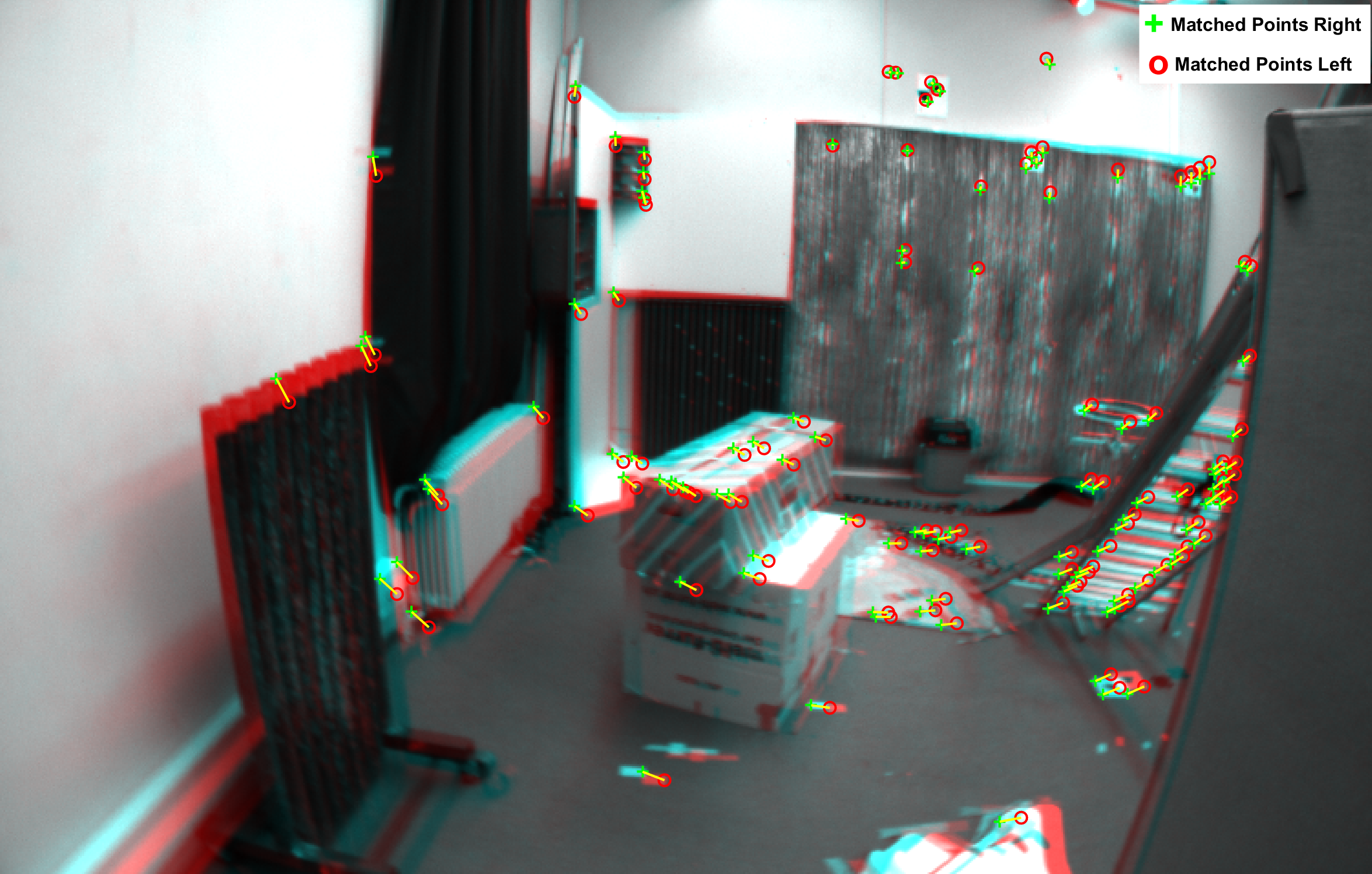
Figure 1: This image presents an example of right and left feature detection and tracking performed by a stereo camera via the Computer Vision System Toolbox with MATLAB R2020b. The annotated photograph is adopted from the EuRoC dataset [21].

Fig. 2 shows the experimental performance of the proposed filter in discrete form. The dataset that was used in this Section is the Vicon Room 2 01 dataset [21]. Fig. 2 presents robust convergence starting from large error in initialization to the neighborhood of the origin. This can be confirmed from the left portion of Fig. 2 which shows accurate tracking performance. Hence, the proposed solution is promising to be implemented on a cheap electronic kit.

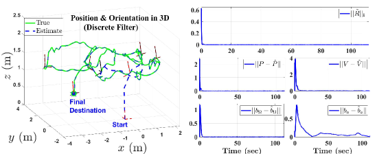
Figure 2: Dataset Vicon Room 2 01: True trajectory versus estimated trajectory plotted using the proposed nonlinear discrete navigation filter. In the right portion, the true trajectory is plotted in green solid-line while the estimated trajectory is plotted in blue dash-line. The true 3-axes orientation is plotted in green solid-line while the estimated orientation is plotted in red dash-line. The final destination is marked with a star. The features are marked by black circles. In the right portion, a blue solid-line is used to demonstrate error components of: orientation $||R\hat{R}^{\top}||_{{\rm I}}$, position $||P-\hat{P}||$, velocity $||V-\hat{V}||$, bias in angular velocity $||b_{\Omega}-\hat{b}_{\Omega}||$, and bias in acceleration $||b_{a}-\hat{b}_{a}||$.

V Conclusion

In this paper, the navigation problem of a vehicle traveling in 3D space has been addressed in deterministic sense. The vehicle’s orientation, position, and linear velocity have been estimated successfully through a proposed nonlinear filter on $\mathbb{SE}_{2}(3)$. The proposed solution successfully accounts and compensates for the unknown bias inevitably present in angular velocity and acceleration measurements. According to the experimental results, the proposed filter showed strong tracking capabilities of the unknown pose and estimation of the unknown linear velocity of the vehicle.

References

- [1] H. A. Hashim, “A geometric nonlinear stochastic filter for simultaneous localization and mapping,” Aerospace Science and Technology, vol. 111, p. 106569, 2021.
- [2] A. I. Mourikis and S. I. Roumeliotis, “A multi-state constraint kalman filter for vision-aided inertial navigation,” in Proceedings 2007 IEEE International Conference on Robotics and Automation. IEEE, 2007, pp. 3565–3572.
- [3] H. A. Hashim, “Gps-denied navigation: Attitude, position, linear velocity, and gravity estimation with nonlinear stochastic observer,” in 2021 American Control Conference (ACC). IEEE, 2021, pp. 1146–1151.
- [4] H. A. Hashim, M. Abouheaf, and M. A. Abido, “Geometric stochastic filter with guaranteed performance for autonomous navigation based on imu and feature sensor fusion,” Control Engineering Practice, vol. PP, no. PP, pp. 1–11, 2021.
- [5] H. A. Hashim, “Systematic convergence of nonlinear stochastic estimators on the special orthogonal group SO(3),” International Journal of Robust and Nonlinear Control, vol. 30, no. 10, pp. 3848–3870, 2020.
- [6] H. A. Hashim, L. J. Brown, and K. McIsaac, “Nonlinear stochastic attitude filters on the special orthogonal group 3: Ito and stratonovich,” IEEE Transactions on Systems, Man, and Cybernetics: Systems, vol. 49, no. 9, pp. 1853–1865, 2019.
- [7] Á. Odry, “An open-source test environment for effective development of marg-based algorithms,” Sensors, vol. 21, no. 4, p. 1183, 2021.
- [8] K. J. Jensen, “Generalized nonlinear complementary attitude filter,” Journal of Guidance, Control, and Dynamics, vol. 34, no. 5, pp. 1588–1593, 2011.
- [9] Á. Odry, R. Fuller, I. J. Rudas, and P. Odry, “Kalman filter for mobile-robot attitude estimation: Novel optimized and adaptive solutions,” Mechanical systems and signal processing, vol. 110, pp. 569–589, 2018.
- [10] H. A. Hashim and F. L. Lewis, “Nonlinear stochastic estimators on the special euclidean group SE(3) using uncertain imu and vision measurements,” IEEE Transactions on Systems, Man, and Cybernetics: Systems, vol. PP, no. PP, pp. 1–14, 2020.
- [11] H. A. Hashim and A. E. E. Eltoukhy, “Landmark and imu data fusion: Systematic convergence geometric nonlinear observer for slam and velocity bias,” IEEE Transactions on Intelligent Transportation Systems, vol. PP, no. PP, pp. 1–10, 2020.
- [12] ——, “Nonlinear filter for simultaneous localization and mapping on a matrix lie group using imu and feature measurements,” IEEE Transactions on Systems, Man, and Cybernetics: Systems, vol. PP, no. PP, pp. 1–12, 2021.
- [13] L. Zhao, H. Qiu, and Y. Feng, “Analysis of a robust kalman filter in loosely coupled gps/ins navigation system,” Measurement, vol. 80, pp. 138–147, 2016.
- [14] Y.-L. Hsu, J.-S. Wang, and C.-W. Chang, “A wearable inertial pedestrian navigation system with quaternion-based extended kalman filter for pedestrian localization,” IEEE Sensors Journal, vol. 17, no. 10, pp. 3193–3206, 2017.
- [15] B. Allotta, A. Caiti, L. Chisci, R. Costanzi, F. Di Corato, C. Fantacci, D. Fenucci, E. Meli, and A. Ridolfi, “An unscented kalman filter based navigation algorithm for autonomous underwater vehicles,” Mechatronics, vol. 39, pp. 185–195, 2016.
- [16] P. M. Blok, K. van Boheemen, F. K. van Evert, J. IJsselmuiden, and G.-H. Kim, “Robot navigation in orchards with localization based on particle filter and kalman filter,” Computers and Electronics in Agriculture, vol. 157, pp. 261–269, 2019.
- [17] A. Barrau and S. Bonnabel, “The invariant extended kalman filter as a stable observer,” IEEE Transactions on Automatic Control, vol. 62, no. 4, pp. 1797–1812, 2016.
- [18] M.-D. Hua and G. Allibert, “Riccati observer design for pose, linear velocity and gravity direction estimation using landmark position and imu measurements,” in 2018 IEEE Conference on Control Technology and Applications (CCTA). IEEE, 2018, pp. 1313–1318.
- [19] H. A. Hashim, “Guaranteed performance nonlinear observer for simultaneous localization and mapping,” IEEE Control Systems Letters, vol. 5, no. 1, pp. 91–96, 2021.
- [20] C. P. Bechlioulis and G. A. Rovithakis, “Robust adaptive control of feedback linearizable mimo nonlinear systems with prescribed performance,” IEEE Transactions on Automatic Control, vol. 53, no. 9, pp. 2090–2099, 2008.
- [21] M. Burri, J. Nikolic, P. Gohl, T. Schneider, J. Rehder, S. Omari, M. W. Achtelik, and R. Siegwart, “The EuRoC micro aerial vehicle datasets,” The International Journal of Robotics Research, vol. 35, no. 10, pp. 1157–1163, 2016.
- [22] H. A. Hashim, “Special orthogonal group SO(3), euler angles, angle-axis, rodriguez vector and unit-quaternion: Overview, mapping and challenges,” arXiv preprint arXiv:1909.06669, 2019.