Residues of bosonic string scattering amplitudes and the Lauricella functions

Abstract

We calculate explicitly residues of all $n$-point Koba-Nielsen (KN) amplitudes by using on-shell recursion relation of string scattering amplitudes (SSA). In addition, we show that the residues of all SSA including the KN amplitudes can be expressed in terms of the Lauricella functions. This result demonstrates the exact $SL(K+3,\mathbb{C})$ symmetry of the tree-level open bosonic string theory. Moreover, we derive an iteration relation among the residues of a given SSA. This iteration relation is related to the $SL(K+3,\mathbb{C})$ symmetry and can presumably be used to soften the well-known hard SSA.

I Introduction

It is known that a string scattering amplitude (SSA) can be expressed in terms of an infinite sum of simple pole terms with residues which are well-organized that its hard high energy behavior is very soft and decays as an exponential fall-off. A well-known simple example is the four tachyon Veneziano amplitude GSW . Presumably, there is a mechanism similar to the symmetry principle in quantum field theory (QFT) which triggers this soft behavior for hard SSA. In contrast to QFT, string theory as a quantum theory of an extended string consists of an infinite number of particles with arbitrary high spins and masses in the spectrum. It is thus reasonable to believe that there exists a huge symmetry group Moore ; Moore1 ; CKT which relates these infinite number of couplings and soften the SSA in the hard scattering limit.

Recently, the present authors calculated a subset of exact $4$-point SSA, namely, amplitudes of three tachyons and one arbitrary string states, and expressed them in terms of the $D$-type Lauricella functions LLY2 . In addition, it was shown that these Lauricella SSA (LSSA) can be expressed in terms of the basis functions in the infinite dimensional representation of the $SL(K+3,C)$ group Group . For any fixed positive integer $K$, one has infinite number of LSSA in the $SL(K+3,C)$ representations slkc . Moreover, it was further shown that there existed $K+2$ recurrence relations among the $D$-type Lauricella functions. These recurrence relations can be used to reproduce the Cartan subalgebra and simple root system of the $SL(K+3,\mathbb{C})$ group with rank $K+2$. As a result, the $SL(K+3,\mathbb{C})$ group with its corresponding stringy Ward identities (recurrence relations) can be used to solve solve all the LSSA and express them in terms of one amplitude. See the recent review LSSA .

The LSSA can be used to rederive the solvability of SSA in various scattering limits LLY2 ,0705 ; RR1 ; RR2 ; RR3 ; RR4 ; RR5 ; RR6 ; RR7 . One important application of this solvability was in the hard string scattering limit. In particular, it was shown that in the hard scattering limit the LSSA can be used to reproduce LLY2 infinite linear relations with constant coefficients among all hard SSA and solve the ratios among them. These behaviors of high energy string scatterings GM ; GM1 ; GrossManes were first conjectured by Gross Gross ; Gross1 and later corrected ChanLee ; ChanLee2 ; CHL and proved ChanLee ; ChanLee2 ; CHLTY2 ; CHLTY1 by the method of decoupling of zero norm states (ZNS) Lee ; lee-Ov ; LeePRL . For details, see the recent review papers review ; over . More importantly, since the decoupling of ZNS and thus the infinite linear relations in the hard scattering limit persist to all string loop orders, it was believed that the proposed $SL(K+3,\mathbb{C})$ symmetry at string-tree level is also valid for string loop amplitudes. On the other hand, one believes that by keeping $M$ fixed as a finite constant in the ZNS calculation, one can obtain more information about the high energy behavior of string theory in contrast to the tensionless string ($\alpha^{\prime}\rightarrow\infty$) approach less1 ; less2 ; less3 ; less5 ; less6 ; less7 ; less8 ; less9 ; less10 ; less11 ; less12 in which all string states are massless.

In this paper, we will apply the string theory extension stringbcfw , bcfw3 ; bcfw4 of field theory BCFW on-shell recursion relations bcfw1 ; bcfw2 to calculate explicitly residues of all $n$-point Koba-Nielsen (KN) amplitudes. In addition, we will show that the residues of all SSA including the KN amplitudes can be expressed in terms of the Lauricella functions. This result demonstrates the exact $SL(K+3,\mathbb{C})$ symmetry of the tree-level open bosonic string theory. On the other hand, since the LSSA of three tachyons and one arbitrary string states can be rederived LLYT from the deformed cubic string field theory (SFT) Taejin , we conjecture that the proposed $SL(K+3,\mathbb{C})$ symmetry can be obtained from Witten SFT.

This paper is organized as following. In section II, we give a brief review of the calculation of the LSSA of three tachyons and one arbitrary string states. In addition, we review the $SL(K+3,\mathbb{C})$ symmetry group and the corresponding recurrence relations of the LSSA. We will then show that SSA of four arbitrary string states can also be written in terms of the Lauricella functions. (details will be given in section V) In section III, we first explicitly calculate the residues of $5$, $6$ and $7$-point KN amplitudes. We then extend the calculation of residues to all $n$-point KN amplitudes. In section IV, we derive an iteration relation among the residues of a given KN amplitude. This iteration relation is related to the $SL(K+3,\mathbb{C})$ symmetry and can presumably be used to soften the well-known hard SSA. In section V, we will first use the shifting method to demonstrate that all $5$-point SSA with arbitrary five tensor legs can be expressed in terms of the LSSA. In general, we can use mathematical induction, together with the on-shell recursion and the shifting principle, to show that all $n$-point SSA can be expressed in terms of the LSSA. We will see that this multi-tensor calculation is closely related to the calculation of applying multi-step string on-shell recursion calculation to KN amplitudes. In section VI, a conclusion and some open questions are given. Finally, in the end an appendix is given to prove some mathematical identities used in the text.

II The Lauricella string scattering amplitudes

In this section we give a brief review of the LSSA of three tachyons and one arbitrary string states in the $26D$ open bosonic string theory and its associated $SL(K+3,C)$ group. The general states at mass level $M_{2}^{2}=2(N_{2}-1)$, $N_{2}=\sum_{n,m,l>0}\left(nr_{n}^{T}+mr_{m}^{P}+lr_{l}^{L}\right)$ with polarizations on the scattering plane can be written as LSSA

$$\left|r_{n}^{T},r_{m}^{P},r_{l}^{L}\right\rangle=\prod_{n>0}\left(\alpha_{-n}^{T}\right)^{r_{n}^{T}}\prod_{m>0}\left(\alpha_{-m}^{P}\right)^{r_{m}^{P}}\prod_{l>0}\left(\alpha_{-l}^{L}\right)^{r_{l}^{L}}|0,k\rangle$$ (2.1)

where $e^{P}=\frac{1}{M_{2}}(E_{2},\mathrm{k}_{2},0)=\frac{k_{2}}{M_{2}}$ the momentum polarization, $e^{L}=\frac{1}{M_{2}}(\mathrm{k}_{2},E_{2},0)$ the longitudinal polarization on and $e^{T}=(0,0,1)$ the transverse polarization. In the CM frame, we define the kinematics as

$$k_{1} =\left(\sqrt{M_{1}^{2}+|\vec{k_{1}}|^{2}},-|\vec{k_{1}}|,0\right),$$ (2.2)

$$k_{2} =\left(\sqrt{M_{2}+|\vec{k_{1}}|^{2}},+|\vec{k_{1}}|,0\right),$$ (2.3)

$$k_{3} =\left(-\sqrt{M_{3}^{2}+|\vec{k_{3}}|^{2}},-|\vec{k_{3}}|\cos\phi,-|\vec{k_{3}}|\sin\phi\right),$$ (2.4)

$$k_{4} =\left(-\sqrt{M_{4}^{2}+|\vec{k_{3}}|^{2}},+|\vec{k_{3}}|\cos\phi,+|\vec{k_{3}}|\sin\phi\right)$$ (2.5)

with $M_{1}^{2}=M_{3}^{2}=M_{4}^{2}=-2$ and $\phi$ is the scattering angle. The Mandelstam variables are defined to be $s=-\left(k_{1}+k_{2}\right)^{2}$, $t=-\left(k_{2}+k_{3}\right)^{2}$ and $u=-\left(k_{1}+k_{3}\right)^{2}$. We will also use the notation $k_{i}^{X}\equiv e^{X}\cdot k_{i}$  for  $X=\left(T,P,L\right).$ It is important to note that SSA of three tachyons and one arbitrary string states with polarizations orthogonal to the scattering plane vanish. It is interesting to note that the $\left(s,t\right)$ channel of the LSSA can be calculated and expressed in terms of the Lauricella functions LSSA

$$A_{st}^{(r_{n}^{T},r_{m}^{P},r_{l}^{L})} =\prod_{n=1}\left[-(n-1)!k_{3}^{T}\right]^{r_{n}^{T}}\cdot\prod_{m=1}\left[-(m-1)!k_{3}^{P}\right]^{r_{m}^{P}}\prod_{l=1}\left[-(l-1)!k_{3}^{L}\right]^{r_{l}^{L}}$$

$$\cdot B\left(-\frac{t}{2}-1,-\frac{s}{2}-1\right)F_{D}^{(K)}\left(-\frac{t}{2}-1;R_{n}^{T},R_{m}^{P},R_{l}^{L};\frac{u}{2}+2-N;\tilde{Z}_{n}^{T},\tilde{Z}_{m}^{P},\tilde{Z}_{l}^{L}\right)$$ (2.6)

where we have defined

$$R_{k}^{X}\equiv\left\{-r_{1}^{X}\right\}^{1},\cdots,\left\{-r_{k}^{X}\right\}^{k}\text{ \ with \ }\left\{a\right\}^{n}=\underset{n}{\underbrace{a,a,\cdots,a}}.$$ (2.7)

and

$$Z_{k}^{X}\equiv\left[z_{1}^{X}\right],\cdots,\left[z_{k}^{X}\right]\text{ \ \ with \ \ }\left[z_{k}^{X}\right]=z_{k0}^{X},\cdots,z_{k\left(k-1\right)}^{X}.$$ (2.8)

In Eq.(2.8), we have defined

$$z_{k}^{X}=\left|\left(-\frac{k_{1}^{X}}{k_{3}^{X}}\right)^{\frac{1}{k}}\right|,\ z_{kk^{\prime}}^{X}=z_{k}^{X}e^{\frac{2\pi ik^{\prime}}{k}},\ \tilde{z}_{kk^{\prime}}^{X}\equiv 1-z_{kk^{\prime}}^{X}\text{ \ \ for \ \ }k^{\prime}=0,\cdots,k-1.$$ (2.9)

In addition to the mass level $M_{2}$ and $N_{2}$, the integer $K$ in Eq.(2.6) is defined to be

$$\text{ }K=\underset{\{\text{for all }r_{j}^{T}\neq 0\}}{\sum j}+\underset{\{\text{for all }r_{j}^{P}\neq 0\}}{\sum j}+\underset{\{\text{for all }r_{j}^{L}\neq 0\}}{\sum j}.$$ (2.10)

The $D$-type Lauricella function $F_{D}^{(K)}$ in Eq.(2.6) is one of the four extensions of the Gauss hypergeometric function to $K$ variables and is defined to be

$$F_{D}^{(K)}\left(\alpha;\beta_{1},...,\beta_{K};\gamma;x_{1},...,x_{K}\right)$$

$$=\sum_{n_{1},\cdots,n_{K}=0}^{\infty}\frac{\left(\alpha\right)_{n_{1}+\cdots+n_{K}}}{\left(\gamma\right)_{n_{1}+\cdots+n_{K}}}\frac{\left(\beta_{1}\right)_{n_{1}}\cdots\left(\beta_{K}\right)_{n_{K}}}{n_{1}!\cdots n_{K}!}x_{1}^{n_{1}}\cdots x_{K}^{n_{K}}$$ (2.11)

where $(\alpha)_{n}=\alpha\cdot\left(\alpha+1\right)\cdots\left(\alpha+n-1\right)$ is the Pochhammer symbol. There was an important integral representation of the Lauricella function Appell

$$F_{D}^{(K)}\left(\alpha;\beta_{1},...,\beta_{K};\gamma;x_{1},...,x_{K}\right)$$

$$=\frac{\Gamma(\gamma)}{\Gamma(\alpha)\Gamma(\gamma-\alpha)}\int_{0}^{1}dt\,t^{\alpha-1}(1-t)^{\gamma-\alpha-1}\cdot(1-x_{1}t)^{-\beta_{1}}(1-x_{2}t)^{-\beta_{2}}...(1-x_{K}t)^{-\beta_{K}},$$ (2.12)

which was used to calculate Eq.(2.6). One can use the LSSA to calculate various scattering limits of the SSA LSSA .

In the following, we discuss the hard scattering limit of the LSSA. For more details, see the recent review LSSA . It was first observed that for each fixed mass level $N$ with $M^{2}=2(N-1)$, the following states are of leading order in energy at the hard scattering limit CHLTY2 ; CHLTY1

$$\left|N,2m,q\right\rangle\equiv(\alpha_{-1}^{T})^{N-2m-2q}(\alpha_{-1}^{L})^{2m}(\alpha_{-2}^{L})^{q}|0,k\rangle.$$ (2.13)

Note that in Eq.(2.13), only even powers $2m$ in $\alpha_{-1}^{L}$ ChanLee ; ChanLee2 survive, and the naive energy order of the amplitudes will drop by an even number of energy powers in general. One important application of the LSSA presented in Eq.(2.6) in the hard string scattering limit is to reproduce LLY2 the infinite linear relations with constant coefficients among all hard SSA and solve the ratios among them LSSA

$$\frac{T^{(N,2m,q)}}{T^{(N,0,0)}}=\left(-\frac{1}{M}\right)^{2m+q}\left(\frac{1}{2}\right)^{m+q}(2m-1)!!.$$ (2.14)

The infinite linear relations with constant coefficients and the solvability of SSA in the hard scattering limit were first conjectured by Gross GM ; GM1 and later corrected ChanLee ; ChanLee2 and proved CHLTY2 ; CHLTY1 by the method of decoupling of zero norm states (ZNS) Lee ; lee-Ov ; LeePRL .

To reproduce the infinite linear relations in Eq.(2.14) from LSSA, we first note that, in the hard scattering limit, the relevant kinematics reduce to

$$k_{1}^{T} =0\text{, \ \ }k_{3}^{T}\simeq-E\sin\phi,$$ (2.15)

$$k_{1}^{L} \simeq-\frac{2p^{2}}{M_{2}}\simeq-\frac{2E^{2}}{M_{2}},$$ (2.16)

$$k_{3}^{L} \simeq\frac{2E^{2}}{M_{2}}\sin^{2}\frac{\phi}{2}$$ (2.17)

where $E$ and $\phi$ are the CM frame energy and scattering angle, respectively. One can calculate

$$\tilde{z}_{kk^{\prime}}^{T}=1,\ \tilde{z}_{kk^{\prime}}^{L}=1-\left(-\frac{s}{t}\right)^{1/k}e^{\frac{i2\pi k^{\prime}}{k}}\sim O\left(1\right),$$ (2.18)

and the LSSA in Eq.(2.6) reduces to LLY2

$$A_{st}^{(r_{n}^{T},r_{l}^{L})}=B\left(-\frac{t}{2}-1,-\frac{s}{2}-1\right)$$

$$\cdot\prod_{n=1}\left[(n-1)!E\sin\phi\right]^{r_{n}^{T}}\prod_{l=1}\left[-(l-1)!\frac{2E^{2}}{M_{2}}\sin^{2}\frac{\phi}{2}\right]^{r_{l}^{L}}$$

$$\cdot F_{D}^{(K)}\left(-\frac{t}{2}-1;R_{n}^{T},R_{l}^{L};\frac{u}{2}+2-N;\left(1\right)_{n},\tilde{Z}_{l}^{L}\right).$$ (2.19)

Since in the hard scattering limit, there was a difference between the naive energy order and the real energy order corresponding to the $\left(\alpha_{-1}^{L}\right)^{r_{1}^{L}}$ operator in Eq.(2.1), it is important to pay attention to the corresponding summation and write

$$A_{st}^{(r_{n}^{T},r_{l}^{L})}=B\left(-\frac{t}{2}-1,-\frac{s}{2}-1\right)$$

$$\cdot\prod_{n=1}\left[(n-1)!E\sin\phi\right]^{r_{n}^{T}}\prod_{l=1}\left[-(l-1)!\frac{2E^{2}}{M_{2}}\sin^{2}\frac{\phi}{2}\right]^{r_{l}^{L}}$$

$$\cdot\sum_{k_{r}}\frac{\left(-\frac{t}{2}-1\right)_{k_{r}}}{\left(\frac{u}{2}+2-N\right)_{k_{r}}}\frac{\left(-r_{1}^{L}\right)_{k_{r}}}{k_{r}!}\left(1+\frac{s}{t}\right)^{k_{r}}\cdot\left(\cdots\right)$$ (2.20)

where $\left(a\right)_{n+m}=\left(a\right)_{n}\left(a+n\right)_{m}$ and $\left(\cdots\right)$ are terms which are not relevant to the following discussion. To proceed, the following formula was proposed LLY2

$$\sum_{k_{r}=0}^{r_{1}^{L}}\frac{\left(-\frac{t}{2}-1\right)_{k_{r}}}{\left(\frac{u}{2}+2-N\right)_{k_{r}}}\frac{\left(-r_{1}^{L}\right)_{k_{r}}}{k_{r}!}\left(1+\frac{s}{t}\right)^{k_{r}}$$

$$= 0\cdot\left(\frac{tu}{s}\right)^{0}\!+0\cdot\left(\frac{tu}{s}\right)^{-1}\!+\dots+0\cdot\left(\frac{tu}{s}\right)^{-\left[\frac{r_{1}^{L}+1}{2}\right]-1}$$

$$+C_{r_{1}^{L}}\left(\frac{tu}{s}\right)^{-\left[\frac{r_{1}^{L}+1}{2}\right]}+\mathit{O}\left\{\left(\frac{tu}{s}\right)^{-\left[\frac{r_{1}^{L}+1}{2}\right]+1}\right\}.$$ (2.21)

where $[$ $]$ stands for the Gauss symbol, $C_{r_{1}^{L}}$ is independent of energy $E$ and depends on $r_{1}^{L}$ and possibly the scattering angle $\phi$. When $r_{1}^{L}=2m$ is an even number, one further proposes that $C_{r_{1}^{L}}=\frac{\left(2m\right)!}{m!}$ and is $\phi$ independent. It was verified that Eq.(2.21) is valid for $r_{1}^{L}=0,1,2,\cdots,10$ LLY2 .

It is interesting to Note that Eq.(2.21) reduces to the Stirling number identity by taking the Regge limit ($s\rightarrow\infty$ with $t$ fixed) and setting $r_{1}^{L}=2m$,

$$\sum_{k_{r}=0}^{2m}\frac{\left(-\frac{t}{2}-1\right)_{k_{r}}}{\left(-\frac{s}{2}\right)_{k_{r}}}\frac{\left(-2m\right)_{k_{r}}}{k_{r}!}\left(\frac{s}{t}\right)^{k_{r}}\simeq\sum_{k_{r}=0}^{2m}\left(-2m\right)_{k_{r}}\left(-\frac{t}{2}-1\right)_{k_{r}}\frac{\left(-2/t\right)^{k_{r}}}{k_{r}!}$$

$$=0\cdot\left(-t\right)^{0}\!+0\cdot\left(-t\right)^{-1}\!+\dots+0\cdot\left(-t\right)^{-m+1}+\frac{(2m)!}{m!}\left(-t\right)^{-m}+\mathit{O}\left\{\left(\frac{1}{t}\right)^{m+1}\right\},$$ (2.22)

which was proposed in KLY and proved in LYAM . The zero terms in Eq.(2.21) correspond to the naive leading energy orders in the hard SSA calculation. In the hard scattering limit, the true leading order SSA can then be identified

$$A_{st}^{(r_{n}^{T},r_{l}^{L})}\simeq B\left(-\frac{t}{2}-1,-\frac{s}{2}-1\right)$$

$$\cdot\prod_{n=1}\left[(n-1)!E\sin\phi\right]^{r_{n}^{T}}\prod_{l=1}\left[-(l-1)!\frac{2E^{2}}{M_{2}}\sin^{2}\frac{\phi}{2}\right]^{r_{l}^{L}}$$

$$\cdot C_{r_{1}^{L}}\left(E\sin\phi\right)^{-2\left[\frac{r_{1}^{L}+1}{2}\right]}\cdot\left(\cdots\right)$$

$$\sim E^{N-\sum_{n\geq 2}nr_{n}^{T}-\left(2\left[\frac{r_{1}^{L}+1}{2}\right]-r_{1}^{L}\right)-\sum_{l\geq 3}lr_{l}^{L}},$$ (2.23)

which means that SSA reaches its highest energy when $r_{n\geq 2}^{T}=r_{l\geq 3}^{L}=0$ and $r_{1}^{L}=2m$, an even number. This result is consistent with the previous result presented in Eq.(2.13).

Finally, the leading order SSA in the hard scattering limit, i.e., $r_{1}^{T}=N-2m-2q$, $r_{1}^{L}=2m$ and $r_{2}^{L}=q$, can be calculated to be LLY2

$$A_{st}^{(N-2m-2q,2m,q)}$$

$$\simeq B\left(-\frac{t}{2}-1,-\frac{s}{2}-1\right)\left(E\sin\phi\right)^{N}\frac{\left(2m\right)!}{m!}\left(-\frac{1}{2M_{2}}\right)^{2m+q}$$

$$=(2m-1)!!\left(-\frac{1}{M_{2}}\right)^{2m+q}\left(\frac{1}{2}\right)^{m+q}A_{st}^{(N,0,0)}$$ (2.24)

which reproduces the ratios in Eq.(2.14).

To obtain the recurrence relations of the Lauricella functions, we consider the type-$1$ Appell functions. For the case of $K=2$, the $D$-type Lauricella functions $F_{D}^{(K)}\left(\alpha;\beta_{1},...,\beta_{K};\gamma;x_{1},...,x_{K}\right)$ reduce to the type-$1$ Appell functions $F_{1}\left(\alpha;\beta_{1},\beta_{2};\gamma,x,y\right)$, and one has $4$ known recurrence relations. It was shown that one can generalize the $4=2+2$ fundamental recurrence relations of the Appell functions $F_{1}$ and prove the following $K+2$ recurrence relations for the $D$-type Lauricella functions $(m=1,2,...,K)$ Group

$$\left(\alpha-\underset{i}{\sum}\beta_{i}\right)F_{D}^{(K)}-\alpha F_{D}^{(K)}\left(\alpha+1\right)+\beta_{1}F_{D}^{(K)}\left(\beta_{1}+1\right)+...+\beta_{K}F_{D}^{(K)}\left(\beta_{K}+1\right) =0,$$ (2.25)

$$\gamma F_{D}^{(K)}-\left(\gamma-\alpha\right)F_{D}^{(K)}\left(\gamma+1\right)-\alpha F_{D}^{(K)}\left(\alpha+1;\gamma+1\right) =0,$$ (2.26)

$$\gamma F_{D}^{(K)}+\gamma(x_{m}-1)F_{D}^{(K)}\left(\beta_{m}+1\right)+(\alpha-\gamma)x_{m}F_{D}^{(K)}\left(\beta_{m}+1,;\gamma+1\right) =0$$ (2.27)

where for simplicity we have omitted those arguments of $F_{D}^{(K)}$ which remain the same in the relations. Moreover, these recurrence relations can be used to reproduce the Cartan subalgebra and simple root system of the $SL(K+3,\mathbb{C})$ group with rank $K+2$Group . As a result, the $SL(K+3,\mathbb{C})$ group with its corresponding stringy Ward identities (recurrence relations) can be used to solve solve all the LSSA and express them in terms of one amplitude.

In particular, it was shown that one can use the above recurrence relations to decrease the value of $K$ step by step and reduce all the Lauricella functions $F_{D}^{(K)}$ in the LSSA to the Gauss hypergeometry functions $F_{D}^{(1)}=$ ${}_{2}F_{1}(\alpha,\beta,\gamma,x)$. One can further reduce the Gauss hypergeometry functions by deriving a multiplication theorem for them, and then solve all the LSSA in terms of one single $4$-tachyon amplitude. One of the reason of this solvability is that all $\beta_{J}$ in the Lauricella functions of the LSSA take very special values, namely, nonpositive integers. See the recent review LSSA .

On the other hand, to obtain the $SL(K+3,\mathbb{C})$ symmetry group of the LSSA, we introduce the variables $a,b_{1},\cdots,b_{K},c$ and define the basis functions slkc

$$f_{ac}^{b_{1}\cdots b_{K}}\left(\alpha;\beta_{1},\cdots,\beta_{K};\gamma;x_{1},\cdots,x_{K}\right)$$

$$=B\left(\gamma-\alpha,\alpha\right)F_{D}^{\left(K\right)}\left(\alpha;\beta_{1},\cdots,\beta_{K};\gamma;x_{1},\cdots,x_{K}\right)a^{\alpha}b_{1}^{\beta_{1}}\cdots b_{K}^{\beta_{K}}c^{\gamma},$$ (2.28)

so that the LSSA in Eq.(2.6) can be written as Group

$$A_{st}^{(r_{n}^{T},r_{m}^{P},r_{l}^{L})}=f_{11}^{-(n-1)!k_{3}^{T},-(m-1)!k_{3}^{P},-(l-1)!k_{3}^{L}}\left(-\frac{t}{2}-1;R_{n}^{T},R_{m}^{P},R_{l}^{L};\frac{u}{2}+2-N;\tilde{Z}_{n}^{T},\tilde{Z}_{m}^{P},\tilde{Z}_{l}^{L}\right).$$ (2.29)

We then define and introduce the $(K+3)^{2}-1$ generators of $SL(K+3,C)$ group slkc ; Group . These are $1$ $E^{\alpha}$, $K$ $E^{\beta_{k}}$, $1$ $E^{\gamma}$,$1$ $E^{\alpha\gamma}$,$K$ $E^{\beta_{k}\gamma}$ and $K$ $E^{\alpha\beta_{k}\gamma}$ which sum up to $3K+3$ raising generators. There are also $3K+3$ lowering operators. In addition, there are $K\left(K-1\right)$ $E_{\beta_{p}}^{\beta_{k}}$ and $K+2$ $\ J$ , $\left\{J_{\alpha},J_{\beta_{k}},J_{\gamma}\right\}$, the Cartan subalgebra. In sum, the total number of generators are $2(3K+3)+K(K-1)+K+2=(K+3)^{2}-1$. The explicit forms of these generators are

$$E^{\alpha} =a\left(\underset{j}{{\displaystyle\sum}}x_{j}\partial_{j}+a\partial_{a}\right),$$

$$E^{\beta_{k}} =b_{k}\left(x_{k}\partial_{k}+b_{k}\partial_{b_{k}}\right),$$

$$E^{\gamma} =c\left(\underset{j}{{\displaystyle\sum}}\left(1-x_{j}\right)\partial_{x_{j}}+c\partial_{c}-a\partial_{a}-\underset{j}{{\displaystyle\sum}}b_{j}\partial_{b_{j}}\right),$$

$$E^{\alpha\gamma} =ac\left(\underset{j}{{\displaystyle\sum}}\left(1-x_{j}\right)\partial_{x_{j}}-a\partial_{a}\right),$$

$$E^{\beta_{k}\gamma} =b_{k}c\left[\left(x_{k}-1\right)\partial_{x_{k}}+b_{k}\partial_{b_{k}}\right],$$

$$E^{\alpha\beta_{k}\gamma} =ab_{k}c\partial_{x_{k}},$$

$$E_{\alpha} =\frac{1}{a}\left[\underset{j}{{\displaystyle\sum}}x_{j}\left(1-x_{j}\right)\partial_{x_{j}}+c\partial_{c}-a\partial_{a}-\underset{j}{{\displaystyle\sum}}x_{j}b_{j}\partial_{b_{j}}\right],$$

$$E_{\beta_{k}} =\frac{1}{b_{k}}\left[x_{k}\left(1-x_{k}\right)\partial_{x_{k}}+x_{k}\underset{j\neq k}{{\displaystyle\sum}}\left(1-x_{j}\right)x_{j}\partial_{x_{j}}+c\partial_{c}-x_{k}a\partial_{a}-\underset{j}{{\displaystyle\sum}}b_{j}\partial_{u_{j}}\right],$$

$$E_{\gamma} =-\frac{1}{c}\left(\underset{j}{{\displaystyle\sum}}x_{j}\partial_{x_{j}}+c\partial_{c}-1\right),$$

$$E_{\alpha\gamma} =\frac{1}{ac}\left[\underset{j}{{\displaystyle\sum}}x_{j}\left(1-x_{j}\right)\partial_{x_{j}}-\underset{j}{{\displaystyle\sum}}x_{j}b_{j}\partial_{b_{j}}+c\partial_{c}-1\right],$$

$$E_{\beta_{k}\gamma} =\frac{1}{b_{k}c}\left[x_{k}\left(x_{k}-1\right)\partial_{x_{k}}+\underset{j\neq k}{{\displaystyle\sum}}\left(x_{j}-1\right)x_{j}\partial_{x_{j}}+x_{k}a\partial_{a}-c\partial_{c}+1\right],$$

$$E_{\alpha\beta_{k}\gamma} =\frac{1}{ab_{k}c}\left[\underset{j}{{\displaystyle\sum}}x_{j}\left(x_{j}-1\right)\partial_{x_{j}}-c\partial_{c}+x_{k}a\partial_{a}+\underset{j}{{\displaystyle\sum}}x_{j}b_{j}\partial_{b_{j}}-x_{k}+1\right],$$

$$E_{\beta_{p}}^{\beta_{k}} =\frac{b_{k}}{b_{p}}\left[\left(x_{k}-x_{p}\right)\partial_{z_{k}}+b_{k}\partial_{b_{k}}\right],(k\neq p),$$

$$J_{\alpha} =a\partial_{a},$$

$$J_{\beta_{k}} =b_{k}\partial_{b_{k}},$$

$$J_{\gamma} =c\partial_{c}.$$ (2.30)

It is straightforward to calculate the operation of these generators on the basis functions ($k=1,2,...K$) $f_{ac}^{b_{1}\cdots b_{K}}\left(\alpha;\beta_{1},\cdots,\beta_{K};\gamma;x_{1},\cdots,x_{K}\right)$

$$E^{\alpha}f_{ac}^{b_{1}\cdots b_{K}}\left(\alpha\right) =\left(\gamma-\alpha-1\right)f_{ac}^{b_{1}\cdots b_{K}}\left(\alpha+1\right),$$

$$E^{\beta_{k}}f_{ac}^{b_{1}\cdots b_{K}}\left(\beta_{k}\right) =\beta_{k}f_{ac}^{b_{1}\cdots b_{K}}\left(\beta_{k}+1\right),$$

$$E^{\gamma}f_{ac}^{b_{1}\cdots b_{K}}\left(\gamma\right) =\left(\gamma-\underset{j}{{\displaystyle\sum}}\beta_{j}\right)f_{ac}^{b_{1}\cdots b_{K}}\left(\gamma+1\right),$$

$$E^{\alpha\gamma}f_{ac}^{b_{1}\cdots b_{K}}\left(\alpha;\gamma\right) =\left(\underset{j}{{\displaystyle\sum}}\beta_{j}-\gamma\right)f_{ac}^{b_{1}\cdots b_{K}}\left(\alpha+1;\gamma+1\right),$$

$$E^{\beta_{k}\gamma}f_{ac}^{b_{1}\cdots b_{K}}\left(\beta_{k};\gamma\right) =\beta_{k}f_{ac}^{b_{1}\cdots b_{K}}\left(\beta_{k}+1;\gamma+1\right),$$

$$E^{\alpha\beta_{k}\gamma}f_{ac}^{b_{1}\cdots b_{K}}\left(\alpha;\beta_{k};\gamma\right) =\beta_{k}f_{ac}^{b_{1}\cdots b_{K}}\left(\alpha+1;\beta_{k}+1;\gamma+1\right),$$

$$E_{\alpha}f_{ac}^{b_{1}\cdots b_{K}}\left(\alpha\right) =\left(\alpha-1\right)f_{ac}^{b_{1}\cdots b_{K}}\left(\alpha-1\right),$$

$$E_{\beta_{k}}f_{ac}^{b_{1}\cdots b_{K}}\left(\beta_{k}\right) =\left(\gamma-\underset{j}{{\displaystyle\sum}}\beta_{j}\right)f_{ac}^{b_{1}\cdots b_{K}}\left(\beta_{k}-1\right),$$

$$E_{\gamma}f_{ac}^{b_{1}\cdots b_{K}}\left(\gamma\right) =\left(\alpha-\gamma+1\right)f_{ac}^{b_{1}\cdots b_{K}}\left(\gamma-1\right),$$

$$E_{\alpha\gamma}f_{ac}^{b_{1}\cdots b_{K}}\left(\alpha;\gamma\right) =\left(\alpha-1\right)f_{ac}^{b_{1}\cdots b_{K}}\left(\alpha-1;\gamma-1\right),$$

$$E_{\beta_{k}\gamma}f_{ac}^{b_{1}\cdots b_{K}}\left(\beta_{k};\gamma\right) =\left(\alpha-\gamma+1\right)f_{ac}^{b_{1}\cdots b_{K}}\left(\beta_{k}-1;\gamma-1\right),$$

$$E_{\alpha\beta_{k}\gamma}f_{ac}^{b_{1}\cdots b_{K}}\left(\alpha;\beta_{k};\gamma\right) =\left(1-\alpha\right)f_{ac}^{b_{1}\cdots b_{K}}\left(\alpha-1;\beta_{k}-1;\gamma-1\right),$$

$$E_{\beta_{p}}^{\beta_{k}}f_{ac}^{b_{1}\cdots b_{K}}\left(\beta_{k};\beta_{p}\right) =\beta_{k}f_{ac}^{b_{1}\cdots b_{K}}\left(\beta_{k}+1;\beta_{p}-1\right),$$

$$J_{\alpha}f_{ac}^{b_{1}\cdots b_{K}}\left(\alpha;\beta_{k};\gamma\right) =\alpha f_{ac}^{b_{1}\cdots b_{K}}\left(\alpha;\beta_{k};\gamma\right),$$

$$J_{\beta_{k}}f_{ac}^{b_{1}\cdots b_{K}}\left(\alpha;\beta_{k};\gamma\right) =\beta_{k}f_{ac}^{b_{1}\cdots b_{K}}\left(\alpha;\beta_{k};\gamma\right),$$

$$J_{\gamma}f_{ac}^{b_{1}\cdots b_{K}}\left(\alpha;\beta_{k};\gamma\right) =\gamma f_{ac}^{b_{1}\cdots b_{K}}\left(\alpha;\beta_{k};\gamma\right)$$ (2.31)

and show explicitly the $SL(K+3,\mathbb{C})$ symmetry of the LSSA LSSA . In Eq.(2.31), we have omitted those arguments in $f_{ac}^{b_{1}\cdots b_{K}}$ that remain the same after the operation. Indeed, with the following identifications slkc

$$E^{\alpha} =\mathcal{E}_{12},E_{\alpha}=\mathcal{E}_{21},E^{\beta_{k}}=\mathcal{E}_{k+3,3},E_{\beta}=\mathcal{E}_{3,k+3},$$

$$E^{\gamma} =\mathcal{E}_{31},E_{\gamma}=\mathcal{E}_{13},E^{\alpha\gamma}=\mathcal{E}_{32},E_{\alpha\gamma}=\mathcal{E}_{23},$$

$$E^{\beta_{k}\gamma} =-\mathcal{E}_{k+3,1},E_{\beta_{k}\gamma}=-\mathcal{E}_{1,k+3},E_{\alpha\beta_{k}\gamma}=-\mathcal{E}_{k+3,2},$$

$$E_{\alpha\beta_{k}\gamma} =-\mathcal{E}_{2,k+3},J_{\alpha}^{\prime}=\frac{1}{2}\left(\mathcal{E}_{11}-\mathcal{E}_{22}\right),J_{\beta_{k}}^{\prime}=\frac{1}{2}\left(\mathcal{E}_{k+3,k+3}-\mathcal{E}_{33}\right),J_{\gamma}^{\prime}=\frac{1}{2}\left(\mathcal{E}_{33}-\mathcal{E}_{11}\right),$$ (2.32)

one can calculate the Lie algebra commutation relations of the $SL(K+3,\mathbb{C})$

$$\left[\mathcal{E}_{ij},\mathcal{E}_{kl}\right]=\delta_{jk}\mathcal{E}_{il}-\delta_{li}\mathcal{E}_{kj};\text{ \ }1\leqslant i,j\leqslant K+3.$$ (2.33)

It is important to note that instead of finite dimensional representation, here we encounter infinite dimensional representation of the noncompact Lie group $SL(K+3,C)$. This means that for any fixed positive integer $K$, one has infinite number of LSSA in the $SL(K+3,C)$ representations.

Finally, it is straightforward to generalize the LSSA of three tachyons and one arbitrary string states and show that all SSA of four arbitrary string states can still be expressed in terms of the $D$-type Lauricella functions $F_{D}^{(K)}.$ See section V for more details. Indeed, for the general multi-tensor $4$-point functions, there are new terms with finite number of contractions among $\partial^{n}X...$ and $\partial^{m}X...$, and one obtains more $D$-type Lauricella functions with different values of $K$. In general, the LSSA of four arbitrary string states can be expressed as sum over finite terms of the $D$-type Lauricella functions and can be written as

$$LSSA=\underset{J}{\sum}c_{J}(k_{i})\int_{0}^{1}dt\,t^{\alpha-1}(1-t)^{\gamma-\alpha-1}\cdot P_{J}(t)$$ (2.34)

where $P_{J}(t)$ is a polynomial with coefficients depending on $k_{i}$ and polarizations $\zeta$, and $c_{J}(k_{i})$ is a $k_{i}$ and $\zeta$ dependent coefficient. One simple example KLT is the two vectors, two tachyons bosonic open SSA

$$A\left(\zeta_{1},k_{1};k_{2};\zeta_{3},k_{3};k_{4}\right) =\left(\zeta_{1}\cdot k_{2}\right)\left(\zeta_{3}\cdot k_{4}\right)\frac{\Gamma\left(\frac{-s}{2}-1\right)\Gamma\left(\frac{-t}{2}-1\right)}{\Gamma\left(-\frac{s}{2}-\frac{t}{2}-2\right)}$$

$$\times F_{D}^{\left(2\right)}\left(\frac{-s}{2}-1;-1,-1;-\frac{s}{2}-\frac{t}{2}-2;-\frac{\zeta_{1}\cdot k_{3}}{\zeta_{1}\cdot k_{2}},-\frac{\zeta_{3}\cdot k_{1}}{\zeta_{3}\cdot k_{4}}\right)$$

$$+\left(\zeta_{1}\cdot\zeta_{3}\right)\frac{\Gamma\left(\frac{-s}{2}\right)\Gamma\left(\frac{-t}{2}\right)}{\Gamma\left(-\frac{s}{2}-\frac{t}{2}\right)}F_{D}^{\left(0\right)}\left(\frac{-s}{2};;-\frac{s}{2}-\frac{t}{2};\right),$$ (2.35)

which contains two Lauricella functions with $K=0,2$. Note that in contrast to Eq.(2.6), all physical polarizations $\zeta_{i}^{\mu}$ except ZNS contribute for the case of multi-tensor SSA as in Eq.(2.35). More examples will be given in section V.

III Residues of the Koba-Nielsen (KN) amplitudes

In this section, we will use the string theory extension bcfw3 ; bcfw4 of field theory BCFW on-shell recursion relations bcfw1 ; bcfw2 to calculate in details the residues of all $n$-point Koba-Nielsen (KN) amplitudes. In section V, we will show that the residues of all $n$-point KN amplitudes calculated in this section can be expressed in terms of the Lauricella functions. Moreover, we will use the shifting principle to show that all SSA including the KN amplitudes can be expressed in terms of the Lauricella functions.

III.1 The Veneziano amplitude

We begin with the discussion on four tachyon amplitude which can be written as

$$A_{4}=\int_{0}^{1}dzz^{k_{1}\cdot k_{2}}\left(1-z\right)^{k_{2}\cdot k_{3}}=\int_{0}^{1}dzz^{k_{1}\cdot k_{2}}e^{k_{2}\cdot k_{3}\ln\left(1-z\right)}=\int_{0}^{1}dzz^{k_{1}\cdot k_{2}}e^{-k_{2}\cdot k_{3}\left(z+\frac{z^{2}}{2}+\frac{z^{3}}{3}+\cdots\right)},$$ (3.1)

or

$$A_{4}=\int_{0}^{1}dzz^{k_{1}\cdot k_{2}}\exp\left[\begin{array}[c]{c}1+T\left(z+\frac{z^{2}}{2}+\frac{z^{3}}{3}+\cdots\right)+\frac{T^{2}}{2}\left(z+\frac{z^{2}}{2}+\frac{z^{3}}{3}+\cdots\right)^{2}\\ +\frac{T^{3}}{3!}\left(z+\frac{z^{2}}{2}+\frac{z^{3}}{3}+\cdots\right)^{3}+\cdots\end{array}\right]$$ (3.4)

$$=\underset{1}{\underbrace{\int_{0}^{1}dzz^{k_{1}\cdot k_{2}}}}+\underset{\alpha_{-1}}{\underbrace{T}}\int_{0}^{1}dzz^{k_{1}\cdot k_{2}+1}+\left(\underset{\alpha_{-2}}{\underbrace{\frac{T}{2}}}+\underset{\alpha_{-1}^{2}}{\underbrace{\frac{T^{2}}{2!}\frac{1}{1^{2}}}}\right)\int_{0}^{1}dzz^{k_{1}\cdot k_{2}+2}$$

$$+\left(\underset{\alpha_{-3}}{\underbrace{\frac{T}{3}}}+\underset{\alpha_{-1}\alpha_{-2}}{\underbrace{\frac{T^{2}}{1!1!}\frac{1}{1^{1}}\frac{1}{2^{1}}}}+\underset{\alpha_{-1}^{3}}{\underbrace{\frac{T^{3}}{3!}}}\right)\int_{0}^{1}dzz^{k_{1}\cdot k_{2}+3}$$

$$+\left(\underset{\alpha_{-4}}{\underbrace{\frac{T}{4}}}+\underset{\alpha_{-3}\alpha_{-1}}{\underbrace{\frac{T^{2}}{1!1!}\frac{1}{1^{1}}\frac{1}{3^{1}}}}+\underset{\alpha_{-2}^{2}}{\underbrace{\frac{T^{2}}{2!}\frac{1}{2^{2}}}}+\underset{\alpha_{-1}^{2}\alpha_{-2}}{\underbrace{\frac{T^{3}}{2!1!}\frac{1}{1^{2}2^{1}}}}+\underset{\alpha_{-1}^{4}}{\underbrace{\frac{T^{4}}{4!}\frac{1}{1^{4}}}}\right)\int_{0}^{1}dzz^{k_{1}\cdot k_{2}+4}+\cdots$$ (3.5)

where $T=-k_{2}\cdot k_{3}$. With the definition of the Mandelstam variables $s=-\left(k_{1}+k_{2}\right)^{2}$, $t=-\left(k_{2}+k_{3}\right)^{2}$, we can express the amplitude in terms of a series of simple pole terms with residues

$$A_{4}=\underset{1}{\underbrace{\frac{2}{-s-2}}}+\underset{\alpha_{-1}}{\underbrace{T\frac{2}{-s+0}}}+(\underset{\alpha_{-2}}{\underbrace{\frac{T}{2}}}+\underset{\alpha_{-1}^{2}}{\underbrace{\frac{T^{2}}{2!}\frac{1}{1^{2}})}}\frac{2}{-s+2}$$

$$+\underset{\alpha_{-3}}{\underbrace{(\frac{T}{3}}}+\underset{\alpha_{-1}\alpha_{-2}}{\underbrace{\frac{T^{2}}{1!1!}\frac{1}{1^{1}}\frac{1}{2^{1}}}}+\underset{\alpha_{-1}^{3}}{\underbrace{\frac{T^{3}}{3!})}}\frac{2}{-s+4}$$

$$\underset{\alpha_{-4}}{\underbrace{(\frac{T}{4}}}+\underset{\alpha_{-3}\alpha_{-1}}{\underbrace{\frac{T^{2}}{1!1!}\frac{1}{1^{1}}\frac{1}{3^{1}}}}+\underset{\alpha_{-2}^{2}}{\underbrace{\frac{T^{2}}{2!}\frac{1}{2^{2}}}}+\underset{\alpha_{-1}^{2}\alpha_{-2}}{\underbrace{\frac{T^{3}}{2!1!}\frac{1}{1^{2}2^{1}}}}+\underset{\alpha_{-1}^{4}}{\underbrace{\frac{T^{4}}{4!}\frac{1}{1^{4}})}}\frac{2}{-s+6}+\cdots$$ (3.6)

$$=\overset{\infty}{\underset{n=0}{\sum}}-\frac{(\alpha(t)+1)(\alpha(t)+2)\cdots(\alpha(t)+n)}{n!}\frac{1}{\alpha(s)-n}$$ (3.7)

where $\alpha(t)=\alpha^{\prime}t+\alpha(0)$ with $\alpha^{\prime}=1/2$ and $\alpha(0)=1$ GSW . In Eq.(3.6) or Eq.(3.5), we can see various residues at each pole of the Veneziano amplitude. We will find generalization of these residues for higher point KN amplitudes in section IV.

III.2 The five-point KN amplitude

For the $5$-point KN amplitude, a simple generalization of Eq.(3.6) is to use the string theory extension stringbcfw of field theory BCFW on-shell recursion relations bcfw1 ; bcfw2 to calculate the infinite number of residues. Moreover, we will show that all residues can be expressed in terms of the Lauricella functions. The $5$-point KN amplitude can be written as stringbcfw

$$A_{5}^{KN} =\int_{0}^{1}dz_{3}\int_{0}^{z_{3}}dz_{2}z_{2}^{k_{2}\cdot k_{1}}z_{3}^{k_{3}\cdot k_{1}}\left(1-z_{3}\right)^{k_{4}\cdot k_{3}}\left(1-z_{2}\right)^{k_{4}\cdot k_{2}}\left(z_{3}-z_{2}\right)^{k_{3}\cdot k_{2}}$$ (3.8)

$$=\underset{a,b,c=0}{\overset{\infty}{{\displaystyle\sum}}}\frac{\left(-k_{2}\cdot k_{3}\right)_{a}}{a!}\frac{\left(-k_{2}\cdot k_{4}\right)_{b}}{b!}\frac{\left(-k_{3}\cdot k_{4}\right)_{c}}{c!}\frac{2}{-s_{12}+2\left(a+b-1\right)}\frac{2}{-s_{123}+2\left(b+c-1\right)}$$ (3.9)

where $s_{12}=-\left(k_{1}+k_{2}\right)^{2},s_{123}=-\left(k_{1}+k_{2}+k_{3}\right)^{2}$. We now consider the BCFW deformation with pair $(k_{1},k_{5})=(1,5)$, and set

$$\hat{k}_{1}\left(z\right)=k_{1}+zq,\hat{k}_{5}\left(z\right)=k_{5}-zq,q^{2}=k_{1}\cdot q=k_{5}\cdot q=0.$$ (3.10)

For $s_{12}$ and $s_{123}$, the poles are located at

$$z_{2,M} =\frac{\left(k_{1}+k_{2}\right)^{2}+2\left(M-1\right)}{-2q\cdot\left(k_{1}+k_{2}\right)},M=a+b=0,1,2,...;$$ (3.11)

$$z_{3,M} =\frac{\left(k_{1}+k_{2}+k_{3}\right)^{2}+2\left(M-1\right)}{-2q\cdot\left(k_{1}+k_{2}+k_{3}\right)},M=b+c=0,1,2,...$$ (3.12)

respectively. By using string on-shell recursion relation, we get stringbcfw

$$A_{5}^{KN}=\underset{M}{\sum}\frac{2}{-s_{12}+2\left(M-1\right)}R_{3,4}^{M}+\underset{{}_{M}}{\sum}\frac{2}{-s_{123}+2\left(M-1\right)}R_{4,3}^{M}$$ (3.13)

where the residues $R_{3,4}^{M}$ and $R_{4,3}^{M}$ can be calculated to be

$$R_{3,4}^{M} =\underset{a,b,c=0,M=a+b}{\overset{\infty}{{\displaystyle\sum}}}\frac{\left(-k_{2}\cdot k_{3}\right)_{a}}{a!}\frac{\left(-k_{2}\cdot k_{4}\right)_{b}}{b!}\frac{\left(-k_{3}\cdot k_{4}\right)_{c}}{c!}\frac{2}{-\hat{s}_{123}\left(z_{N}\right)+2\left(b+c-1\right)},$$ (3.14)

$$R_{4,3}^{M} =\underset{a,b,c=0,M=b+c}{\overset{\infty}{{\displaystyle\sum}}}\frac{\left(-k_{2}\cdot k_{3}\right)_{a}}{a!}\frac{\left(-k_{2}\cdot k_{4}\right)_{b}}{b!}\frac{\left(-k_{3}\cdot k_{4}\right)_{c}}{c!}\frac{2}{-\hat{s}_{12}\left(w_{M}\right)+2\left(a+b-1\right)}.$$ (3.15)

The residues $R_{3,4}^{M}$ and $R_{4,3}^{M}$ above can be further calculated to be

$$R_{3,4}^{M} =\underset{a,b=0,M=a+b}{\overset{\infty}{{\displaystyle\sum}}}\frac{\left(-k_{2}\cdot k_{3}\right)_{a}}{a!}\frac{\left(-k_{2}\cdot k_{4}\right)_{b}}{b!}\int_{0}^{1}dz_{2}z_{2}^{\left(\hat{k}_{1}+k_{2}\right)\cdot k_{3}-a}\left(1-z_{2}\right)^{k_{3}\cdot k_{4}},$$ (3.16)

$$R_{4,3}^{M} =\underset{b,c=0,M=b+c}{\overset{\infty}{{\displaystyle\sum}}}\frac{\left(-k_{2}\cdot k_{4}\right)_{b}}{b!}\frac{\left(-k_{3}\cdot k_{4}\right)_{c}}{c!}\int_{0}^{1}dz_{2}z_{2}^{\hat{k}_{1}\cdot k_{2}+b}\left(1-z_{2}\right)^{k_{2}\cdot k_{3}}.$$ (3.17)

We can now use the identity derived in the appendix

$$\underset{b+c=M,b,c=0}{\sum}\frac{\left(T_{1}\right)_{b}}{b!}\frac{\left(T_{2}\right)_{c}}{c!}x_{1}^{b}x_{2}^{c}=\underset{\left\{N_{r}\right\}}{\sum}\prod_{r=1}\left(\frac{1}{N_{r}!r^{N_{r}}}\left[T_{1}x_{1}^{r}+T_{2}x_{2}^{r}\right]^{N_{r}}\right)$$ (3.18)

to obtain

$$R_{3,4}^{M} =\underset{\left\{N_{r}\right\}}{\sum}\left(-k_{2}\cdot k_{3}\right)^{N}\int_{0}^{1}dz_{2}z_{2}^{\left(\hat{k}_{1}+k_{2}\right)\cdot k_{3}-M}\left(1-z_{2}\right)^{k_{3}\cdot k_{4}}\prod_{r=1}\frac{1}{N_{r}!r^{N_{r}}}\left[1-\left(-\frac{k_{2}\cdot k_{4}}{k_{2}\cdot k_{3}}\right)z_{2}^{r}\right]^{N_{r}},$$ (3.19)

$$R_{4,3}^{M} =\underset{\left\{N_{r}\right\}}{\sum}\left(-k_{3}\cdot k_{4}\right)^{N}\int_{0}^{1}dz_{2}z_{2}^{\hat{k}_{1}\cdot k_{2}}\left(1-z_{2}\right)^{k_{2}\cdot k_{3}}\prod_{r=1}\frac{1}{N_{r}!r^{N_{r}}}\left[1-\left(-\frac{k_{2}\cdot k_{4}}{k_{3}\cdot k_{4}}\right)z_{2}^{r}\right]^{N_{r}}.$$ (3.20)

In Eq.(3.19) and Eq.(3.20) the sums are over partitions of $N$ into $\left\{N_{r}\right\}$ with $M=\underset{r=1}{\sum}rN_{r}$ and $N=\underset{r=1}{\sum}N_{r}$. Thus the string on-shell recursion relation reduces the $5$-point KN amplitude into two products of subamplitudes $3\otimes 4$ and $4\otimes 3$ with $3$-point and $4$-point functions. One can now easily express the residues in Eq.(3.19) and Eq.(3.20) in terms of sums of the Lauricella functions

$$R_{3,4}^{M} =\underset{\left\{N_{r}\right\}}{\sum}\left(-k_{2}\cdot k_{3}\right)^{N}B\left(\left(\hat{k}_{1}+k_{2}\right)\cdot k_{3}-M+1,k_{3}\cdot k_{4}+1\right)\left(\prod_{r=1}\frac{1}{N_{r}!r^{N_{r}}}\right)$$

$$\cdot F_{D}^{(K)}\left(\begin{array}[c]{c}\left(\hat{k}_{1}+k_{2}\right)\cdot k_{3}-M+1;\cdots,\left\{-N_{r}\right\}^{r},\cdots;\\ \left(\hat{k}_{1}+k_{2}\right)\cdot k_{3}+k_{3}\cdot k_{4}-M+2;\cdots,\left[\left(-\frac{k_{2}\cdot k_{4}}{k_{2}\cdot k_{3}}\right)_{r}\right],\cdots\end{array}\right),$$ (3.23)

$$R_{4,3}^{M} =\underset{\left\{N_{r}\right\}}{\sum}\left(-k_{3}\cdot k_{4}\right)^{N}B\left(\hat{k}_{1}\cdot k_{2}+1,k_{2}\cdot k_{3}+1\right)\left(\prod_{r=1}\frac{1}{N_{r}!r^{N_{r}}}\right)$$

$$\cdot F_{D}^{(K)}\left(\begin{array}[c]{c}\hat{k}_{1}\cdot k_{2}+1;\cdots,\left\{-N_{r}\right\}^{r},\cdots;\\ \hat{k}_{1}\cdot k_{2}+k_{2}\cdot k_{3}+2;\cdots,\left[\left(-\frac{k_{2}\cdot k_{4}}{k_{3}\cdot k_{4}}\right)_{r}\right],\cdots\end{array}\right).$$ (3.26)

where $K=\underset{\{\text{for all }N_{r}\neq 0\}}{\sum r}$.

III.3 The six-point KN amplitude

For the higher $n$-point KN amplitudes, we define the residues $R_{m+1,n-m+1}^{M}$ ($2\leq m\leq n-2$) of $n$-point KN amplitude and express the KN amplitude as

$$A_{n}^{KN}=\underset{m=2}{\overset{n-2}{\sum}}\underset{M=0}{\overset{\infty}{\sum}}\frac{2R_{m+1,n-m+1}^{M}}{\left(k_{1}+k_{2}+...+k_{m}\right)^{2}+2(M-1)}$$ (3.27)

where the pole locations $z_{m,M}$ are given by solutions of

$$\left(\hat{k}_{1}+k_{2}+....+k_{m}\right)^{2}+2(M-1)=0,M=0,1,2...\text{.}$$ (3.28)

Figure 1: Residues of KN amplitudes

For the case of $6$-point KN amplitude. There are three types of residues $R_{3,5}^{M}$, $R_{4,4}^{M}$ and $R_{5,3}^{M}$. For the residue $R_{3,5}^{M}$, we propose the left and right subamplitudes as following

$$A\left(\hat{1},2,-P\right)=R_{3,5}^{P,L}=\prod_{r=1}\frac{\underset{\sigma=1}{\overset{N_{r}}{{\displaystyle\prod}}}\epsilon_{r}^{(\sigma)}\cdot k_{2}}{\sqrt{N_{r}!r^{N_{r}}}},$$ (3.29)

$$A\left(P,3,4,5,\hat{6}\right)=R_{3,5}^{P,R}$$

$$=\int_{0}^{1}dw_{4}\int_{0}^{w_{4}}dw_{3}w_{3}^{k_{P}\cdot k_{3}}w_{4}^{k_{P}\cdot k_{4}}\left(1-w_{3}\right)^{k_{3}\cdot k_{5}}\left(1-w_{4}\right)^{k_{4}\cdot k_{5}}\left(w_{4}-w_{3}\right)^{k_{3}\cdot k_{4}}$$

$$\times\prod_{r=1}\frac{1}{\sqrt{N_{r}!r^{N_{r}}}}\underset{\sigma=1}{\overset{N_{r}}{{\displaystyle\prod}}}\left(-\epsilon_{r}^{(\sigma)}\right)\cdot\left[k_{3}\left(\frac{1}{w_{3}}\right)^{r}+k_{4}\left(\frac{1}{w_{4}}\right)^{r}+k_{5}\left(\frac{1}{1}\right)^{r}\right].$$ (3.30)

where $k_{P}=\hat{k}_{1}+k_{2}$ and $P$ is a normalized arbitrary string fock state

$$\left|P\right\rangle=\prod_{r=1}\frac{\left(\underset{\sigma=1}{\overset{N_{r}}{{\displaystyle\prod}}}\epsilon_{r}^{(\sigma)}\cdot\alpha_{-r}\right)}{\sqrt{N_{r}!r^{Nr}}}\left|0,k_{P}\right\rangle.$$ (3.31)

In Eq.(3.31), it is understood, for example, that the state $\epsilon_{1}^{(1)}\cdot\alpha_{-1}\epsilon_{1}^{(2)}\cdot\alpha_{-1}\epsilon_{1}^{(3)}\cdot\alpha_{-1}$ means $\epsilon_{\mu\nu\lambda}\alpha_{-1}^{\mu}\alpha_{-1}^{\nu}\alpha_{-1}^{\lambda}$. In Eq.(3.29), we have chosen $z_{1}=0$, $z_{2}=1$ and $z_{P}=\infty$ to fix the $SL(2,R)$ gauge. Similarly, in Eq.(3.30), we set $w_{P}=0$, $w_{5}=1$ and $w_{6}=\infty$. After summing over all $P$, we obtain the residue

$$R_{3,5}^{M}=\underset{\left\{N_{r}\right\}}{\sum}\int_{0}^{1}dw_{4}\int_{0}^{w_{4}}dw_{3}w_{3}^{\left(\hat{k}_{1}+k_{2}\right)\cdot k_{3}}w_{4}^{\left(\hat{k}_{1}+k_{2}\right)\cdot k_{4}}\left(1-w_{3}\right)^{k_{3}\cdot k_{5}}\left(1-w_{4}\right)^{k_{4}\cdot k_{5}}\left(w_{4}-w_{3}\right)^{k_{3}\cdot k_{4}}$$

$$\times\prod_{r=1}\frac{\left[\left(-k_{2}\cdot k_{3}\right)\left(\frac{1}{w_{3}}\right)^{r}+\left(-k_{2}\cdot k_{4}\right)\left(\frac{1}{w_{4}}\right)^{r}+\left(-k_{2}\cdot k_{5}\right)\left(\frac{1}{1}\right)^{r}\right]}{N_{r}!r^{N_{r}}}^{N_{r}}.$$ (3.32)

For the residue $R_{4,4}^{M}$, we propose the left and right subamplitudes as following

$$A\left(\hat{1},2,3,-P\right) =R_{4,4}^{P,L}=\prod_{r=1}\int_{0}^{1}dz_{2}z_{2}^{\hat{k}_{1}\cdot k_{2}}\left(1-z_{2}\right)^{k_{2}\cdot k_{3}}\frac{\underset{\sigma=1}{\overset{N_{r}}{{\displaystyle\prod}}}\epsilon_{r}^{(\sigma)}\cdot\left[k_{2}\left(z_{2}\right)^{r}+k_{3}\left(1\right)^{r}\right]}{\sqrt{N_{r}!r^{N_{r}}}},$$ (3.33)

$$A\left(P,4,5,\hat{6}\right) =R_{4,4}^{P,R}=\prod_{r=1}\int_{0}^{1}dw_{4}w_{4}^{k_{P}\cdot k_{4}}\left(1-w_{4}\right)^{k_{4}\cdot k_{5}}\frac{\underset{\sigma=1}{\overset{N_{r}}{{\displaystyle\prod}}}\left(-\epsilon_{r}^{(\sigma)}\right)\cdot\left[k_{4}\left(\frac{1}{w_{4}}\right)^{r}+k_{5}\left(\frac{1}{1}\right)^{r}\right]}{\sqrt{N_{r}!r^{N_{r}}}}$$ (3.34)

where $k_{P}=\hat{k}_{1}+k_{2}+k_{3}$. In Eq.(3.33), we have chosen $z_{1}=0$, $z_{3}=1$ and $z_{P}=\infty$ to fix the $SL(2,R)$ gauge. Similarly, in Eq.(3.34), we set $w_{P}=0$, $w_{5}=1$ and $w_{6}=\infty$. After summing over all $P$, we obtain the residue

$$R_{4,4}^{M} =\underset{\left\{N_{r}\right\}}{\sum}\int_{0}^{1}dw_{4}\int_{0}^{1}dz_{2}z_{2}^{\hat{k}_{1}\cdot k_{2}}\left(1-z_{2}\right)^{k_{2}\cdot k_{3}}w_{4}^{\left(\hat{k}_{1}+k_{2}+k_{3}\right)\cdot k_{4}}\left(1-w_{4}\right)^{k_{4}\cdot k_{5}}$$

$$\times\prod_{r=1}\frac{\left[\left(-k_{2}\cdot k_{4}\right)\left(\frac{z_{2}}{w_{4}}\right)^{r}+\left(-k_{2}\cdot k_{5}\right)\left(z_{2}\right)^{r}+\left(-k_{3}\cdot k_{4}\right)\left(\frac{1}{w_{4}}\right)^{r}+\left(-k_{3}\cdot k_{5}\right)1^{r}\right]^{N_{r}}}{N_{r}!r^{N_{r}}},$$ (3.35)

which is a sum of products of the Lauricella functions after term by term integrations for a given $M$. On the other hand, to prove that the residue $R_{3,5}^{M}$ in Eq.(3.32) (and the residue $R_{5,3}^{M}$ to be discussed below) can be expressed in terms of LSSA, one needs to do a second on-shell recursion process. This will be done in section V.

For the residue $R_{5,3}^{M}$, we propose the left and right subamplitudes as following

$$A\left(-P,5,\hat{6}\right)=R_{5,3}^{P,R}=\prod_{r=1}\frac{\left(-\underset{\sigma=1}{\overset{N_{r}}{{\displaystyle\prod}}}\epsilon_{r}^{(\sigma)}\cdot k_{5}\right)}{\sqrt{N_{r}!r^{N_{r}}}}$$ (3.36)

$$A\left(\hat{1},2,3,4,P\right)=R_{5,3}^{P,L}$$

$$=\int_{0}^{1}dz_{3}\int_{0}^{z_{3}}dz_{2}z_{2}^{\hat{k}_{1}\cdot k_{2}}z_{3}^{\hat{k}_{1}\cdot k_{3}}\left(z_{3}-z_{2}\right)^{k_{2}\cdot k_{3}}\left(1-z_{2}\right)^{k_{2}\cdot k_{4}}\left(1-z_{3}\right)^{k_{3}\cdot k_{4}}$$

$$\times\prod_{r=1}\frac{\underset{\sigma=1}{\overset{N_{r}}{{\displaystyle\prod}}}\epsilon_{r}^{(\sigma)}\cdot\left[k_{2}\left(z_{2}\right)^{r}+k_{3}\left(z_{3}\right)^{r}+k_{4}\left(1\right)^{r}\right]}{\sqrt{N_{r}!r^{N_{r}}}}$$ (3.37)

where we have chosen $z_{1}=0$, $z_{4}=1$ and $z_{P}=\infty$ to fix the $SL(2,R)$ gauge. Similarly, in Eq.(3.36), we set $w_{P}=0$, $w_{5}=1$ and $w_{6}=\infty$. After summing over all $P$, we can get

$$R_{5,3}^{M} =\underset{\left\{N_{r}\right\}}{\sum}\int_{0}^{1}dz_{3}\int_{0}^{z_{3}}dz_{2}z_{2}^{\hat{k}_{1}\cdot k_{2}}z_{3}^{\hat{k}_{1}\cdot k_{3}}\left(z_{3}-z_{2}\right)^{k_{2}\cdot k_{3}}\left(1-z_{2}\right)^{k_{2}\cdot k_{4}}\left(1-z_{3}\right)^{k_{3}\cdot k_{4}}$$

$$\times\prod_{r=1}\frac{\left[\left(-k_{2}\cdot k_{5}\right)\left(z_{2}\right)^{r}+\left(-k_{3}\cdot k_{5}\right)\left(z_{3}\right)^{r}+\left(-k_{4}\cdot k_{5}\right)\left(1\right)^{r}\right]^{N_{r}}}{N_{r}!r^{N_{r}}}.$$ (3.38)

To justify the results in Eq.(3.32), Eq.(3.35) and Eq.(3.38), we follow the standard string on-shell recursion calculation. The $6$-point KN amplitude can be written as

$$A_{6}^{KN}=\int_{0}^{1}dz_{4}\int_{0}^{z_{4}}dz_{3}\int_{0}^{z_{3}}dz_{2}z_{2}^{k_{1}\cdot k_{2}}z_{3}^{k_{1}\cdot k_{3}}z_{4}^{k_{1}\cdot k_{4}}$$

$$\cdot\left(z_{3}-z_{2}\right)^{k_{2}\cdot k_{3}}\left(z_{4}-z_{2}\right)^{k_{2}\cdot k_{4}}\left(1-z_{2}\right)^{k_{2}\cdot k_{5}}\left(z_{4}-z_{3}\right)^{k_{3}\cdot k_{4}}\left(1-z_{3}\right)^{k_{3}\cdot k_{5}}$$

$$=\underset{a,b,c,d,e,f=0}{\sum}\frac{\left(-k_{2}\cdot k_{3}\right)_{a}}{a!}\frac{\left(-k_{2}\cdot k_{4}\right)_{b}}{b!}\frac{\left(-k_{2}\cdot k_{5}\right)_{c}}{c!}\frac{\left(-k_{3}\cdot k_{4}\right)_{d}}{d!}\frac{\left(-k_{3}\cdot k_{5}\right)_{e}}{e!}\frac{\left(-k_{4}\cdot k_{5}\right)_{f}}{f!}$$

$$\times\frac{2}{\left(-s_{12}\right)+2\left(a+b+c-1\right)}\frac{2}{\left(-s_{123}\right)+2\left(b+c+d+e-1\right)}\frac{2}{\left(-s_{1234}\right)+2\left(c+e+f-1\right)}$$ (3.39)

where

$$s_{12}=-\left(k_{1}+k_{2}\right)^{2},s_{123}=-\left(k_{1}+k_{2}+k_{3}\right)^{2},s_{1234}=-\left(k_{1}+k_{2}+k_{3}+k_{4}\right)^{2}.$$ (3.40)

The next step is to do the on-shell recursion deformation

$$\hat{k}_{1}\left(z\right)=k_{1}+zq,q^{2}=k_{1}\cdot q=k_{6}\cdot q=0,\hat{k}_{6}\left(z\right)=k_{6}-zq$$ (3.41)

to obtain the poles

$$z_{2,M} =\frac{\left(k_{1}+k_{2}\right)^{2}+2\left(M-1\right)}{-2q\cdot\left(k_{1}+k_{2}\right)},M=a+b+c=0,1,2,...;$$ (3.42)

$$z_{3,M} =\frac{\left(k_{1}+k_{2}+k_{3}\right)^{2}+2\left(M-1\right)}{-2q\cdot\left(k_{1}+k_{2}+k_{3}\right)},M=b+c+d+e=0,1,2,...;$$ (3.43)

$$z_{4,M} =\frac{\left(k_{1}+k_{2}+k_{3}+k_{4}\right)^{2}+2\left(M-1\right)}{-2q\cdot\left(k_{1}+k_{2}+k_{3}+k_{4}\right)},M=c+e+f=0,1,2,....$$ (3.44)

The amplitude can then be written as

$$A_{6}^{KN}=\underset{M}{\sum}\frac{2}{\left(-s_{12}\right)+2\left(M-1\right)}R_{3,5}^{M}+\underset{M}{\sum}\frac{2}{\left(-s_{123}\right)+2\left(M-1\right)}R_{4,4}^{M}+\underset{M}{\sum}\frac{2}{\left(-s_{1234}\right)+2\left(M-1\right)}R_{5,3}^{M}$$ (3.45)

where the residues can be calculated to be

$$R_{3,5}^{M}=\underset{\begin{array}[c]{c}a,b,c,d,e,f=0\\ M=a+b+c\end{array}}{\sum}\frac{\left(-k_{2}\cdot k_{3}\right)_{a}}{a!}\frac{\left(-k_{2}\cdot k_{4}\right)_{b}}{b!}\frac{\left(-k_{2}\cdot k_{5}\right)_{c}}{c!}\frac{\left(-k_{3}\cdot k_{4}\right)_{d}}{d!}\frac{\left(-k_{3}\cdot k_{5}\right)_{e}}{e!}\frac{\left(-k_{4}\cdot k_{5}\right)_{f}}{f!}$$ (3.48)

$$\times\frac{2}{\left(-\hat{s}_{123}\left(z_{2,M}\right)\right)+2\left(b+c+d+e-1\right)}\frac{2}{\left(-\hat{s}_{1234}\left(z_{2,M}\right)\right)+2\left(c+e+f-1\right)},$$ (3.49)

$$R_{4,4}^{M}=\underset{\begin{array}[c]{c}a,b,c,d,e,f=0\\ M=b+c+d+e\end{array}}{\sum}\frac{\left(-k_{2}\cdot k_{3}\right)_{a}}{a!}\frac{\left(-k_{2}\cdot k_{4}\right)_{b}}{b!}\frac{\left(-k_{2}\cdot k_{5}\right)_{c}}{c!}\frac{\left(-k_{3}\cdot k_{4}\right)_{d}}{d!}\frac{\left(-k_{3}\cdot k_{5}\right)_{e}}{e!}\frac{\left(-k_{4}\cdot k_{5}\right)_{f}}{f!}$$ (3.52)

$$\times\frac{2}{\left(-\hat{s}_{12}\left(z_{3,M}\right)\right)+2\left(a+b+c-1\right)}\frac{2}{\left(-\hat{s}_{1234}\left(z_{3,M}\right)\right)+2\left(c+e+f-1\right)},$$ (3.53)

$$R_{5,3}^{M}=\underset{\begin{array}[c]{c}a,b,c,d,e,f=0\\ M=c+e+f\end{array}}{\sum}\frac{\left(-k_{2}\cdot k_{3}\right)_{a}}{a!}\frac{\left(-k_{2}\cdot k_{4}\right)_{b}}{b!}\frac{\left(-k_{2}\cdot k_{5}\right)_{c}}{c!}\frac{\left(-k_{3}\cdot k_{4}\right)_{d}}{d!}\frac{\left(-k_{3}\cdot k_{5}\right)_{e}}{e!}\frac{\left(-k_{4}\cdot k_{5}\right)_{f}}{f!}$$ (3.56)

$$\times\frac{2}{\left(-\hat{s}_{12}\left(z_{4,M}\right)\right)+2\left(a+b+c-1\right)}\frac{2}{\left(-\hat{s}_{123}\left(z_{4,M}\right)\right)+2\left(b+c+d+e-1\right)}.$$ (3.57)

Finally, we need to identify Eq.(3.32) with Eq.(3.49), Eq.(3.35) with Eq.(3.53) and Eq.(3.38) with Eq.(3.57) respectively. To do this on the residue $R_{3,5}^{M}$, we apply Eq.(A.16) for the case of $n=3$ and rewrite Eq.(3.32) as

$$R_{3,5}^{M}=\int_{0}^{1}dw_{4}\int_{0}^{w_{4}}dw_{3}w_{3}^{\left(\hat{k}_{1}+k_{2}\right)\cdot k_{3}}w_{4}^{\left(\hat{k}_{1}+k_{2}\right)\cdot k_{4}}\left(1-w_{3}\right)^{k_{3}\cdot k_{5}}\left(1-w_{4}\right)^{k_{4}\cdot k_{5}}\left(w_{4}-w_{3}\right)^{k_{3}\cdot k_{4}}$$

$$\times\underset{\begin{array}[c]{c}M=a+b+c\\ a,b,c=0\end{array}}{\sum}\frac{\left(-k_{2}\cdot k_{3}\right)_{a}}{a!}\frac{\left(-k_{2}\cdot k_{4}\right)_{b}}{b!}\frac{\left(-k_{2}\cdot k_{5}\right)_{c}}{c!}w_{3}^{-a}w_{4}^{-b}1^{-c},$$ (3.60)

which after binormal expansions and integrations can be further written as

$$R_{3,5}^{M} =\underset{\begin{array}[c]{c}M=a+b+c\\ a,b,c,d,e,f=0\end{array}}{\sum}\frac{\left(-k_{2}\cdot k_{3}\right)_{a}}{a!}\frac{\left(-k_{2}\cdot k_{4}\right)_{b}}{b!}\frac{\left(-k_{2}\cdot k_{5}\right)_{c}}{c!}\frac{\left(-k_{3}\cdot k_{4}\right)_{d}}{d!}\frac{\left(-k_{3}\cdot k_{5}\right)_{e}}{e!}\frac{\left(-k_{4}\cdot k_{5}\right)_{f}}{f!}$$ (3.63)

$$\times\frac{1}{\left(\hat{k}_{1}+k_{2}\right)\cdot k_{3}+(d+e-a+1)}\frac{1}{\left(\hat{k}_{1}+k_{2}\right)\cdot\left(k_{3}+k_{4}\right)+k_{3}\cdot k_{4}+\left(e+f-a+2\right)}.$$ (3.64)

We see that Eq.(3.64) above is the same as Eq.(3.49) since

$$2\left(\hat{k}_{1}+k_{2}\right)\cdot k_{3}+2\left(d+e-a+1\right)=\left(-\hat{s}_{123}\left(z_{2,M}\right)\right)+2\left(b+c+d+e-1\right)$$ (3.65)

and

$$2\left(\hat{k}_{1}+k_{2}\right)\cdot\left(k_{3}+k_{4}\right)+2k_{3}\cdot k_{4}+2\left(e+f-a+2\right)=\left(-\hat{s}_{1234}\left(z_{2,M}\right)\right)+2\left(c+e+f-1\right).$$ (3.66)

This completes the proof that the proposals of the subamplitudes in Eq.(3.29), Eq.(3.30) and thus the result of the residue calculated in Eq.(3.32) are indeed the correct ones.

For the residue $R_{4,4}^{M}$, we apply Eq.(A.16) for the case of $n=4$ and rewrite Eq.(3.35) as

$$R_{4,4}^{M} =\int_{0}^{1}dw_{4}\int_{0}^{1}dz_{2}z_{2}^{\hat{k}_{1}\cdot k_{2}}\left(1-z_{2}\right)^{k_{2}\cdot k_{3}}w_{4}^{\left(\hat{k}_{1}+k_{2}+k_{3}\right)\cdot k_{4}}\left(1-w_{4}\right)^{k_{4}\cdot k_{5}}$$

$$\underset{\begin{array}[c]{c}b,c,d,e=0\\ M=b+c+d+e\end{array}}{\sum}\frac{\left(-k_{2}\cdot k_{4}\right)_{b}}{b!}\frac{\left(-k_{2}\cdot k_{5}\right)_{c}}{c!}\frac{\left(-k_{3}\cdot k_{4}\right)_{d}}{d!}\frac{\left(-k_{3}\cdot k_{5}\right)_{e}}{e!}\left(\frac{z_{2}}{w_{4}}\right)^{b}\left(z_{2}\right)^{c}\left(\frac{1}{w_{4}}\right)^{d}$$ (3.69)

which after binomial expansions and integrations can be further written as

$$R_{4,4}^{M} =\underset{\begin{array}[c]{c}M=b+c+d+e\\ a,b,c,d,e,f=0\end{array}}{\sum}\frac{\left(-k_{2}\cdot k_{3}\right)_{a}}{a!}\frac{\left(-k_{2}\cdot k_{4}\right)_{b}}{b!}\frac{\left(-k_{2}\cdot k_{5}\right)_{c}}{c!}\frac{\left(-k_{3}\cdot k_{4}\right)_{d}}{d!}\frac{\left(-k_{3}\cdot k_{5}\right)_{e}}{e!}\frac{\left(-k_{4}\cdot k_{5}\right)_{f}}{f!}$$ (3.72)

$$\times\frac{1}{\hat{k}_{1}\cdot k_{2}+\left(a+b+c+1\right)}\frac{1}{\left(\hat{k}_{1}+k_{2}+k_{3}\right)\cdot k_{4}+\left(f-b-d+1\right)}.$$ (3.73)

We see that Eq.(3.73) above is the same as Eq.(3.53) since

$$-\hat{s}_{12}\left(z_{3,M}\right)+2\left(a+b+c-1\right)=2\hat{k}_{1}\cdot k_{2}+2\left(a+b+c+1\right)$$ (3.74)

and

$$-\hat{s}_{1234}(z_{3,M})+2\left(c+e+f-1\right)=2\left(\hat{k}_{1}+k_{2}+k_{3}\right)\cdot k_{4}+2\left(f-b-d+1\right).$$ (3.75)

This completes the proof that the proposals of the subamplitudes in Eq.(3.33), Eq.(3.34) and thus the result of the residue calculated in Eq.(3.35) are indeed the correct ones.

For the residue $R_{5,3}^{M}$, we apply Eq.(A.16) for the case of $n=3$ and rewrite Eq.(3.38) as

$$R_{5,3}^{M} =\int_{0}^{1}dz_{3}\int_{0}^{z_{3}}dz_{2}z_{2}^{\hat{k}_{1}\cdot k_{2}}z_{3}^{\hat{k}_{1}\cdot k_{3}}\left(z_{3}-z_{2}\right)^{k_{2}\cdot k_{3}}\left(1-z_{2}\right)^{k_{2}\cdot k_{4}}\left(1-z_{3}\right)^{k_{3}\cdot k_{4}}$$

$$\underset{\begin{array}[c]{c}M=c+e+f\\ c,e,f=0\end{array}}{\sum}\frac{\left(-k_{2}\cdot k_{5}\right)_{c}}{c!}\frac{\left(-k_{3}\cdot k_{5}\right)_{e}}{e!}\frac{\left(-k_{4}\cdot k_{5}\right)_{f}}{f!}\left(z_{2}\right)^{c}\left(z_{3}\right)^{e}\left(1\right)^{f},$$ (3.78)

which after binomial expansions and integrations can be further written as

$$R_{5,3}^{M} =\underset{\begin{array}[c]{c}M=c+e+f\\ a,b,c,d,e,f=0\end{array}}{\sum}\frac{\left(-k_{2}\cdot k_{3}\right)_{a}}{a!}\frac{\left(-k_{2}\cdot k_{4}\right)_{b}}{b!}\frac{\left(-k_{2}\cdot k_{5}\right)_{c}}{c!}\frac{\left(-k_{3}\cdot k_{4}\right)_{c}}{d!}\frac{\left(-k_{3}\cdot k_{5}\right)_{e}}{e!}\frac{\left(-k_{4}\cdot k_{5}\right)_{f}}{f!}$$ (3.81)

$$\times\frac{1}{\hat{k}_{1}\cdot k_{2}+a+b+c+1}\frac{1}{\hat{k}_{1}\cdot k_{2}+\hat{k}_{1}\cdot k_{3}+k_{2}\cdot k_{3}+b+c+d+e+2}$$ (3.82)

We see that Eq.(3.82) above is the same as Eq.(3.57) since

$$-\hat{s}_{12}\left(z_{4,M}\right)+2\left(a+b+c-1\right)=2\hat{k}_{1}\cdot k_{2}+2\left(a+b+c+1\right)$$ (3.83)

and

$$-\hat{s}_{123}\left(z_{4,M}\right)+2\left(b+c+d+e-1\right)=2\hat{k}_{1}\cdot k_{2}+2\hat{k}_{1}\cdot k_{3}+2k_{2}\cdot k_{3}+2(b+c+d+e+2).$$ (3.84)

This completes the proof that the proposals of the subamplitudes in Eq.(3.37), Eq.(3.36) and thus the result of the residue calculated in Eq.(3.38) are indeed the correct ones.

III.4 The seven-point KN amplitude

For the case of $7$-point KN amplitude. There are four types of residues $R_{3,6}^{M}$, $R_{4,5}^{M}$, $R_{5,4}^{M}$ and $R_{6,3}^{M}$. We will work out residues $R_{3,6}^{M}$and $R_{4,5}^{M}$. Similar calculation can be done for $R_{5,4}^{M}$ and $R_{6,3}^{M}$. For the residue $R_{3,6}^{M}$, we propose the left and right subamplitudes as following

$$A\left(\hat{1},2,-P\right)=R_{3,6}^{P,L}=\prod_{r=1}\frac{\left(\underset{\sigma=1}{\overset{N_{r}}{{\displaystyle\prod}}}\epsilon_{r}^{(\sigma)}\cdot k_{2}\right)}{\sqrt{N_{r}!r^{N_{r}}}},$$ (3.85)

$$A\left(P,3,4,5,6,\hat{7}\right)=R_{3,6}^{P,R}$$

$$=\int_{0}^{1}dw_{5}\int_{0}^{w_{5}}dw_{4}\int_{0}^{w_{4}}dw_{3}w_{3}^{k_{P}\cdot k_{3}}w_{4}^{k_{P}\cdot k_{4}}w_{5}^{\left(\hat{k}_{1}+k_{2}\right)\cdot k_{5}}\left(1-w_{3}\right)^{k_{3}\cdot k_{6}}\left(1-w_{4}\right)^{k_{4}\cdot k_{6}}$$

$$\cdot\left(1-w_{5}\right)^{k_{5}\cdot k_{6}}\left(w_{4}-w_{3}\right)^{k_{3}\cdot k_{4}}\left(w_{5}-w_{3}\right)^{k_{3}\cdot k_{5}}\left(w_{5}-w_{4}\right)^{k_{4}\cdot k_{5}}$$

$$\times\prod_{r=1}\frac{1}{\sqrt{N_{r}!r^{N_{r}}}}\underset{\sigma=1}{\overset{N_{r}}{{\displaystyle\prod}}}\left(-\epsilon_{r}^{(\sigma)}\right)\cdot\left[k_{3}\left(\frac{1}{w_{3}}\right)^{r}+k_{4}\left(\frac{1}{w_{4}}\right)^{r}+k_{5}\left(\frac{1}{w_{5}}\right)^{r}+k_{6}\left(\frac{1}{1}\right)^{r}\right]$$ (3.86)

where $P$ is a normalized arbitrary string fock state defined in Eq.(3.31) and $k_{P}=\hat{k}_{1}+k_{2}$. In Eq.(3.85), we have chosen $z_{1}=0$, $z_{2}=1$ and $z_{P}=\infty$ to fix the $SL(2,R)$ gauge. Similarly, in Eq.(3.86), we set $w_{P}=0$, $w_{6}=1$ and $w_{7}=\infty$. After summing over all $P$, we obtain the residue

$$R_{3,6}^{M}=\underset{\left\{N_{r}\right\}}{\sum}\int_{0}^{1}dw_{5}\int_{0}^{w_{5}}dw_{4}\int_{0}^{w_{4}}dw_{3}w_{3}^{\left(\hat{k}_{1}+k_{2}\right)\cdot k_{3}}w_{4}^{\left(\hat{k}_{1}+k_{2}\right)\cdot k_{4}}w_{5}^{\left(\hat{k}_{1}+k_{2}\right)\cdot k_{5}}$$

$$\cdot\left(1-w_{3}\right)^{k_{3}\cdot k_{5}}\left(1-w_{4}\right)^{k_{4}\cdot k_{5}}\left(w_{4}-w_{3}\right)^{k_{3}\cdot k_{4}}$$

$$\times\prod_{r=1}\frac{\left[\left(-k_{2}\cdot k_{3}\right)\left(\frac{1}{w_{3}}\right)^{r}+\left(-k_{2}\cdot k_{4}\right)\left(\frac{1}{w_{4}}\right)^{r}+\left(-k_{2}\cdot k_{5}\right)\left(\frac{1}{w_{5}}\right)^{r}+\left(-k_{2}\cdot k_{6}\right)\left(\frac{1}{1}\right)^{r}\right]}{N_{r}!r^{N_{r}}}^{N_{r}}.$$ (3.87)

To justify the result in Eq.(3.87), we follow the standard string on-shell recursion calculation. First of all, we use the identity Eq.(A.16) to transform the last line of Eq.(3.87) to a summation, and then do binomial expansions before performing integrations. Finally we end up with

$$R_{3,6}^{M} =\underset{\begin{array}[c]{c}M=a+b+c+d\\ a,b,c,d,e,f,g,h,i,j=0\end{array}}{\sum}\frac{\left(-k_{2}\cdot k_{3}\right)_{a}}{a!}\frac{\left(-k_{2}\cdot k_{4}\right)_{b}}{b!}\frac{\left(-k_{2}\cdot k_{5}\right)_{c}}{c!}\frac{\left(-k_{2}\cdot k_{6}\right)_{d}}{d!}$$ (3.90)

$$\cdot\frac{\left(-k_{3}\cdot k_{4}\right)_{e}}{e!}\frac{\left(-k_{3}\cdot k_{5}\right)_{f}}{f!}\frac{\left(-k_{3}\cdot k_{6}\right)_{g}}{g!}\frac{\left(-k_{4}\cdot k_{5}\right)_{h}}{h!}\frac{\left(-k_{4}\cdot k_{6}\right)_{i}}{i!}\frac{\left(-k_{5}\cdot k_{6}\right)_{j}}{j!}$$

$$\times\frac{1}{\left(\hat{k}_{1}+k_{2}\right)\cdot k_{3}+(e+f+g-a+1)}\frac{1}{\left(\hat{k}_{1}+k_{2}\right)\cdot\left(k_{3}+k_{4}\right)+k_{3}\cdot k_{4}+\left(f+g+h+i-a-b+2\right)}$$

$$\times\frac{1}{\left(\hat{k}_{1}+k_{2}\right)\cdot\left(k_{3}+k_{4}+k_{5}\right)+k_{3}\cdot k_{4}+k_{3}\cdot k_{5}+k_{4}\cdot k_{5}+\left(g+i+j-a-b-c+3\right)}.$$ (3.91)

On the other hand, the residue $R_{3,6}^{M}$ can be extracted from the pole of the $7$-point KN amplitude

$$z_{2,M}=\frac{\left(k_{1}+k_{2}\right)^{2}+2\left(M-1\right)}{-2q\cdot\left(k_{1}+k_{2}\right)},M=a+b+c+d=0,1,2,...\text{,}$$ (3.92)

and calculated to be

$$R_{3,6}^{M} =\underset{\begin{array}[c]{c}M=a+b+c+d\\ a,b,c,d,e,f,g,h,i,j=0\end{array}}{\sum}\frac{\left(-k_{2}\cdot k_{3}\right)_{a}}{a!}\frac{\left(-k_{2}\cdot k_{4}\right)_{b}}{b!}\frac{\left(-k_{2}\cdot k_{5}\right)_{c}}{c!}\frac{\left(-k_{2}\cdot k_{6}\right)_{d}}{d!}$$ (3.95)

$$\cdot\frac{\left(-k_{3}\cdot k_{4}\right)_{e}}{e!}\frac{\left(-k_{3}\cdot k_{5}\right)_{f}}{f!}\frac{\left(-k_{3}\cdot k_{6}\right)_{g}}{g!}\frac{\left(-k_{4}\cdot k_{5}\right)_{h}}{h!}\frac{\left(-k_{4}\cdot k_{6}\right)_{i}}{i!}\frac{\left(-k_{5}\cdot k_{6}\right)_{j}}{j!}$$

$$\times\frac{2}{-\hat{s}_{123}\left(z_{2,M}\right)+2\left(b+c+d+e+f+g-1\right)}\frac{2}{-\hat{s}_{1234}\left(z_{2,M}\right)+2\left(c+d+f+g+h+i-1\right)}$$

$$\times\frac{2}{-\hat{s}_{12345}\left(z_{2,M}\right)+2\left(d+g+i+j-1\right)}.$$ (3.96)

It is straightforwad to verify

$$-\hat{s}_{123}\left(z_{2,M}\right)+2\left(b+c+d+e+f+g-1\right) =2\left(\hat{k}_{1}+k_{2}\right)\cdot k_{3}+2(e+f+g-a+1),$$ (3.97)

$$-\hat{s}_{1234}\left(z_{2,M}\right)+2\left(c+d+f+g+h+i-1\right) =2\left(\hat{k}_{1}+k_{2}\right)\cdot\left(k_{3}+k_{4}\right)+2k_{3}\cdot k_{4}$$

$$+2\left(f+g+h+i-a-b+2\right),$$ (3.98)

$$-\hat{s}_{12345}\left(z_{2,M}\right)+2\left(d+g+i+j-1\right) =2\left(\hat{k}_{1}+k_{2}\right)\cdot\left(k_{3}+k_{4}+k_{5}\right)+2k_{3}\cdot k_{4}+2k_{3}\cdot k_{5}$$

$$+2k_{4}\cdot k_{5}+2\left(g+i+j-a-b-c+3\right).$$ (3.99)

This shows that Eq.(3.91) is the same as Eq.(3.96), and the proposal in Eq.(3.85) and Eq.(3.86) are consistent ones.

For the residue $R_{4,5}^{M}$, we propose the left and right subamplitudes as following

$$A\left(\hat{1},2,3,-P\right) =R_{4,5}^{P,L}=\prod_{r=1}\int_{0}^{1}dz_{2}z_{2}^{\hat{k}_{1}\cdot k_{2}}\left(1-z_{2}\right)^{k_{2}\cdot k_{3}}\frac{\underset{\sigma=1}{\overset{N_{r}}{{\displaystyle\prod}}}\epsilon_{r}^{(\sigma)}\cdot\left[k_{2}\left(z_{2}\right)^{r}+k_{3}\left(1\right)^{r}\right]}{\sqrt{N_{r}!r^{N_{r}}}},$$ (3.100)

$$A\left(P,4,5,6,\hat{7}\right) =R_{4,5}^{P,R}=\prod_{r=1}\int_{0}^{1}dw_{4}\int_{0}^{w_{4}}dw_{5}w_{4}^{k_{P}\cdot k_{4}}w_{5}^{k_{P}\cdot k_{5}}\left(1-w_{4}\right)^{k_{4}\cdot k_{6}}\left(1-w_{5}\right)^{k_{5}\cdot k_{6}}\left(w_{5}-w_{4}\right)^{k_{4}\cdot k_{5}}$$

$$\times\frac{\underset{\sigma=1}{\overset{N_{r}}{{\displaystyle\prod}}}\left(-\epsilon_{r}^{(\sigma)}\right)\cdot\left[k_{4}\left(\frac{1}{w_{4}}\right)^{r}+k_{5}\left(\frac{1}{w_{5}}\right)^{r}+k_{6}\left(\frac{1}{1}\right)^{r}\right]}{\sqrt{N_{r}!r^{N_{r}}}}$$ (3.101)

where $k_{P}=\hat{k}_{1}+k_{2}+k_{3}$. After summing over all $P$, we obtain the residue

$$R_{4,5}^{M} =\underset{\left\{N_{r}\right\}}{\sum}\int_{0}^{1}dw_{4}\int_{0}^{w_{4}}dw_{5}\int_{0}^{1}dz_{2}z_{2}^{\hat{k}_{1}\cdot k_{2}}\left(1-z_{2}\right)^{k_{2}\cdot k_{3}}w_{4}^{k_{P}\cdot k_{4}}w_{5}^{k_{P}\cdot k_{5}}\left(1-w_{4}\right)^{k_{4}\cdot k_{6}}\left(1-w_{5}\right)^{k_{5}\cdot k_{6}}\left(w_{5}-w_{4}\right)^{k_{4}\cdot k_{5}}$$

$$\times\prod_{r=1}\frac{\left[\begin{array}[c]{c}\left(-k_{2}\cdot k_{4}\right)\left(\frac{z_{2}}{w_{4}}\right)^{r}+\left(-k_{2}\cdot k_{5}\right)\left(\frac{z_{2}}{w_{5}}\right)^{r}+\left(-k_{2}\cdot k_{6}\right)\left(z_{2}\right)^{r}\\ +\left(-k_{3}\cdot k_{4}\right)\left(\frac{1}{w_{4}}\right)^{r}+\left(-k_{3}\cdot k_{5}\right)\left(\frac{1}{w_{5}}\right)^{r}+\left(k_{3}\cdot k_{6}\right)\left(\frac{1}{1}\right)^{r}\end{array}\right]^{N_{r}}}{N_{r}!r^{N_{r}}}.$$ (3.104)

The next step is to use the identity in Eq.(A.16) and then do binomial expansions before performing integrations on Eq.(3.104), we finally end up with

$$R_{4,5}^{M} =\underset{\begin{array}[c]{c}M=b+c+d+e+f+g\\ a,b,c,d,e,f,g,h,i,j=0\end{array}}{\sum}\frac{\left(-k_{2}\cdot k_{3}\right)_{a}}{a!}\frac{\left(-k_{2}\cdot k_{4}\right)_{b}}{b!}\frac{\left(-k_{2}\cdot k_{5}\right)_{c}}{c!}\frac{\left(-k_{2}\cdot k_{6}\right)_{d}}{d!}$$ (3.107)

$$\cdot\frac{\left(-k_{3}\cdot k_{4}\right)_{e}}{e!}\frac{\left(-k_{3}\cdot k_{5}\right)_{f}}{f!}\frac{\left(-k_{3}\cdot k_{6}\right)_{g}}{g!}\frac{\left(-k_{4}\cdot k_{5}\right)_{h}}{h!}\frac{\left(-k_{4}\cdot k_{6}\right)_{i}}{i!}\frac{\left(-k_{5}\cdot k_{6}\right)_{j}}{j!}$$

$$\times\frac{1}{\left(\hat{k}_{1}+k_{2}+k_{3}\right)\cdot k_{4}+(h+i-b-e+1)}$$

$$\times\frac{1}{\left(\hat{k}_{1}+k_{2}+k_{3}\right)\cdot\left(k_{4}+k_{5}\right)+k_{4}\cdot k_{5}+\left(i+j-b-c-e-f+2\right)}$$

$$\times\frac{1}{\hat{k}_{1}\cdot k_{2}+\left(a+b+c+d+1\right)}.$$ (3.108)

On the other hand, the residue $R_{4,5}^{M}$ can be extracted from the pole of the $7$-point KN amplitude

$$z_{3,M}=\frac{\left(k_{1}+k_{2}+k_{3}\right)^{2}+2\left(M-1\right)}{-2q\cdot\left(k_{1}+k_{2}+k_{3}\right)},M=b+c+d+e+f+g=0,1,2,...\text{,}$$ (3.109)

and calculated to be

$$R_{4,5}^{M} =\underset{\begin{array}[c]{c}M=b+c+d+e+f+g\\ a,b,c,d,e,f,g,h,i,j=0\end{array}}{\sum}\frac{\left(-k_{2}\cdot k_{3}\right)_{a}}{a!}\frac{\left(-k_{2}\cdot k_{4}\right)_{b}}{b!}\frac{\left(-k_{2}\cdot k_{5}\right)_{c}}{c!}\frac{\left(-k_{2}\cdot k_{6}\right)_{d}}{d!}$$ (3.112)

$$\cdot\frac{\left(-k_{3}\cdot k_{4}\right)_{e}}{e!}\frac{\left(-k_{3}\cdot k_{5}\right)_{f}}{f!}\frac{\left(-k_{3}\cdot k_{6}\right)_{g}}{g!}\frac{\left(-k_{4}\cdot k_{5}\right)_{h}}{h!}\frac{\left(-k_{4}\cdot k_{6}\right)_{i}}{i!}\frac{\left(-k_{5}\cdot k_{6}\right)_{j}}{j!}$$

$$\times\frac{1}{-\hat{s}_{1234}\left(z_{3,M}\right)+2\left(c+d+f+g+h+i-1\right)}$$

$$\times\frac{1}{-\hat{s}_{12345}\left(z_{3,M}\right)+2\left(d+g+i+j-1\right)}\times\frac{1}{-\hat{s}_{12}\left(z_{3,M}\right)+2\left(a+b+c+d-1\right)}.$$ (3.113)

It is straightforward to verify

$$-\hat{s}_{1234}\left(z_{3,M}\right)+2\left(c+d+f+g+h+i-1\right) =2\left(\hat{k}_{1}+k_{2}+k_{3}\right)\cdot k_{4}+2(h+i-b-e+1),$$ (3.114)

$$-\hat{s}_{12345}\left(z_{3,M}\right)+2\left(d+g+i+j-1\right) =2\left(\hat{k}_{1}+k_{2}+k_{3}\right)\cdot\left(k_{4}+k_{5}\right)+2k_{4}\cdot k_{5}$$

$$+2\left(i+j-b-c-e-f+2\right),$$ (3.115)

$$-\hat{s}_{12}\left(z_{3,M}\right)+2\left(a+b+c+d-1\right) =2\hat{k}_{1}\cdot k_{2}+2\left(a+b+c+d+1\right).$$ (3.116)

This shows that Eq.(3.108) is the same as Eq.(3.113), and the proposal in Eq.(3.100) and Eq.(3.101) are consistent ones.

III.5 The n-point KN amplitude

In this section, we will adopt two methods to calculate the residues of general $n$-point KN amplitudes. We will first use the method of subamplitudes similar to the previous subsections. We then use a direct calculation method. The result that residues of all $n$-point SSA can be expressed in terms of Lauricella functions will be discussed in section V.

III.5.1 Method of subamplitudes

To calculate the residues $R_{m+1,n-m+1}^{M}$ of $A_{n}$ in Eq.(3.27), we can generalize the previous calculations and propose the following two subamplitudes $R_{m+1,n-m+1}^{P,L}\left(\hat{1},2,...,m,-P\right)$ and $R_{m+1,n-m+1}^{P,R}\left(P,m+1,\cdots,n-1,\hat{n}\right)$

$$R_{m+1,n-m+1}^{P,L}\left(\underset{z_{1}=0}{\underbrace{\hat{1}}},\underset{z_{2}}{\underbrace{2}},\cdots,\underset{z_{m-1}}{\underbrace{m-1}},\underset{z_{m}=1}{\underbrace{m}},\underset{\infty}{\underbrace{-P}}\right)$$

$$=\int_{0}^{1}dz_{m-1}\cdots\int_{0}^{z_{3}}dz_{2}\underset{1\leq j<i\leq m}{\prod}\left(z_{i}-z_{j}\right)^{k_{i}\cdot k_{j}}\prod_{r=1}\frac{\left[\underset{\sigma=1}{\overset{N_{r}}{{\displaystyle\prod}}}\epsilon_{r}^{(\sigma)}\cdot\underset{2\leq i\leq m}{\sum}k_{i}\left(z_{i}\right)^{r}\right]}{\sqrt{N_{r}!r^{N_{r}}}},$$ (3.117)

$$R_{m+1,n-m+1}^{P,R}\left(\underset{w_{m}=0}{\underbrace{P}},\underset{{}_{w_{m+1}}}{\underbrace{m+1}},\cdots,\underset{w_{n-2}}{\underbrace{n-2}},\underset{w_{n-1}=1}{\underbrace{n-1}},\underset{w_{n}=\infty}{\underbrace{\hat{n}}}\right)$$

$$=\int_{0}^{1}dw_{n-2}\cdots\int_{0}^{w_{m+2}}dw_{m+1}\underset{P=m\leq j<i\leq n-1}{\prod}\left(w_{i}-w_{j}\right)^{k_{i}\cdot k_{j}}\prod_{r=1}\frac{\left[\underset{\sigma=1}{\overset{N_{r}}{{\displaystyle\prod}}}\left(-\epsilon_{r}^{(\sigma)}\right)\cdot\underset{m+1\leq i\leq n-1}{\sum}k_{i}\left(\frac{1}{w_{i}}\right)^{r}\right]}{\sqrt{N_{r}!r^{N_{r}}}}$$ (3.118)

where $k_{P}=\hat{k}_{1}+\underset{i=2}{\overset{m}{\sum}}k_{i}$. It is understood that $k_{1}$ in Eq.(3.117) should be replaced by $\hat{k}_{1}$.

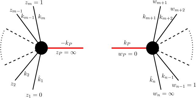
Figure 2: The left and right subamplitudes

We then sum over all $P$ to obtain the residue

$$R_{m+1,n-m+1}^{M}\left(\hat{1},2,\cdots,m,m+1,\cdots,n-1,\hat{n}\right)$$

$$=\int_{0}^{1}dz_{m-1}\cdots\int_{0}^{z_{3}}dz_{2}\int_{0}^{1}dw_{n-2}\cdots\int_{0}^{w_{m+2}}dw_{m+1}\underset{1\leq j<i\leq m}{\prod}\left(z_{i}-z_{j}\right)^{k_{i}\cdot k_{j}}$$

$$\times\underset{P=m\leq j<i\leq n-1}{\prod}\left(w_{i}-w_{j}\right)^{k_{i}\cdot k_{j}}\underset{\left\{N_{r}\right\}}{\sum}\prod_{r=1}\frac{\left[\underset{2\leq j\leq m,m+1\leq i\leq n-1}{\sum}\left(-k_{j}\cdot k_{i}\right)\left(\frac{z_{j}}{w_{i}}\right)^{r}\right]}{N_{r}!r^{N_{r}}}^{N_{r}}.$$ (3.119)

We will show in section V that all residues $R_{m+1,n-m+1}^{M}$ in Eq.(3.119) can be expressed in terms of sum over LSSA.

III.5.2 Direct calculation

In the previous method of subamplitudes calculation, we did not do a consistency check similar to Eq.(3.114), Eq.(3.115) and Eq.(3.116). In this section, we adopt a direct calculation starting from the general $n$-point KN amplitude. The $n$-point KN amplitude is

$$A_{n}^{KN}=\int_{0}^{1}dz_{n-2}\int_{0}^{z_{n-2}}dz_{n-3}\cdots\int_{0}^{z_{3}}dz_{2}\text{ }\prod_{i>j=1}^{n-2}\left(z_{i}-z_{j}\right)^{k_{i}\cdot k_{j}}\text{, }z_{i}\geq z_{j}$$ (3.120)

which has $\left(n-3\right)$ series of poles for each integral on $z_{2},\cdots,z_{n-2}$.

To investigate the poles for the integral on $z_{m}$, which splits the $n$-point Koba-Nielsen amplitude to a $\left(m+1\right)$-point and a $\left(n-m+1\right)$-point amplitudes connected by a string propagator, we express $A_{n}^{KN}$ in the following form

$$A_{n}^{KN} =\int_{0}^{1}dz_{n-2}\cdots\int_{0}^{z_{m+2}}dz_{m+1}\int_{0}^{z_{m+1}}dz_{m}\int_{0}^{z_{m}}dz_{m-1}\cdots\int_{0}^{z_{3}}dz_{2}$$

$$\cdot\prod_{m\geq i>j}\left(z_{i}-z_{j}\right)^{k_{i}\cdot k_{j}}\prod_{i>j>m}\left(z_{i}-z_{j}\right)^{k_{i}\cdot k_{j}}\prod_{i>m\geq j}\left(z_{i}-z_{j}\right)^{k_{i}\cdot k_{j}}$$ (3.121)

where we have taken $\left(z_{0},z_{n-1},z_{n}\right)=\left(0,1,\infty\right)$ to fix the $SL\left(2,R\right)$ invariance.

By defining the new coordinates,

$$\text{for }i >m:y_{i}=z_{i}\text{ with }\left(y_{m}\equiv y_{P},y_{n-1},y_{n}\right)=\left(0,1,\infty\right),$$ (3.122)

$$\text{for }i =m:z_{P}=\frac{z_{m}}{z_{m+1}},$$ (3.123)

$$\text{for }i <m:x_{i}=\frac{z_{i}}{z_{m}}\text{ with }\left(x_{1},x_{m},x_{m+1}\right)=\left(0,1,\infty\right),$$ (3.124)

Eq.(3.121) becomes

$$A_{n}^{KN} =\int_{0}^{1}dy_{n-2}\cdots\int_{0}^{y_{m+2}}dy_{m+1}\text{ }\prod_{i=m+1}^{n-2}y_{i}^{k_{i}\cdot k_{P}}\prod_{i>j=m+1}^{n-2}\left(y_{i}-y_{j}\right)^{k_{i}\cdot k_{j}}$$

$$\times\int_{0}^{1}dx_{m-1}\cdots\int_{0}^{x_{3}}dx_{2}\text{ }\prod_{i>j=1}^{m-1}\left(x_{i}-x_{j}\right)^{k_{i}\cdot k_{j}}$$

$$\times\int_{0}^{1}dz_{P}\text{ }\left(z_{P}\right)^{\sum\limits_{m\geq i>j}k_{i}\cdot k_{j}+m-2}\left(y_{m+1}\right)^{\sum\limits_{m\geq i>j}k_{i}\cdot k_{j}+m-1}\prod_{2\leq j\leq m,m+1\leq i\leq n-1}\left(1-\frac{y_{m+1}z_{P}x_{j}}{y_{i}}\right)^{k_{i}\cdot k_{j}}.$$ (3.125)

We then expand the last product in Eq.(3.125) by using Binomial theorem

$$\left(1-\frac{y_{m+1}z_{P}x_{j}}{y_{i}}\right)^{k_{i}\cdot k_{j}}=\sum_{a_{ij}}\frac{\left(-k_{i}\cdot k_{j}\right)_{a_{ij}}}{a_{ij}!}\left(\frac{y_{m+1}z_{P}x_{j}}{y_{i}}\right)^{a_{ij}}$$ (3.126)

where $a_{ij}$’s are integers, to get

$$A_{n}^{KN} =\int_{0}^{1}dy_{n-2}\cdots\int_{0}^{y_{m+2}}dy_{m+1}\text{ }\underset{P=m\leq j<i\leq n-1}{\prod}\left(y_{i}-y_{j}\right)^{k_{i}\cdot k_{j}}$$

$$\times\int_{0}^{1}dx_{m-1}\cdots\int_{0}^{x_{3}}dx_{2}\text{ }\underset{1\leq j<i\leq m}{\prod}\left(x_{i}-x_{j}\right)^{k_{i}\cdot k_{j}}\sum_{a_{ij}}\left(y_{m+1}\right)^{\sum\limits_{m\geq i>j}k_{i}\cdot k_{j}+\sum\limits_{2\leq j\leq m,m+1\leq i\leq n-1}a_{ij}+m-1}$$

$$\times\prod_{2\leq j\leq m,m+1\leq i\leq n-1}\frac{\left(-k_{i}\cdot k_{j}\right)_{a_{ij}}}{a_{ij}!}\left(\frac{x_{j}}{y_{i}}\right)^{a_{ij}}\int_{0}^{1}dz_{P}\text{ }\left(z_{P}\right)^{\sum\limits_{m\geq i>j}k_{i}\cdot k_{j}\sum\limits_{2\leq j\leq m,m+1\leq i\leq n-1}a_{ij}+m-2}.$$ (3.127)

In the above calculation, we have defined the momentum of the propagator as $k_{P}=\sum\limits_{j=1}^{m}k_{j}$.

By performing the integral on $z_{P}$, we finally express $A_{n}^{KN}$ in the following form

$$A_{n}^{KN} =\int_{0}^{1}dy_{n-2}\cdots\int_{0}^{y_{m+2}}dy_{m+1}\text{ }\underset{P=m\leq j<i\leq n-1}{\prod}\left(y_{i}-y_{j}\right)^{k_{i}\cdot k_{j}}$$

$$\times\int_{0}^{1}dx_{m-1}\cdots\int_{0}^{x_{3}}dx_{2}\text{ }\underset{1\leq j<i\leq m}{\prod}\left(x_{i}-x_{j}\right)^{k_{i}\cdot k_{j}}\sum_{a_{ij}}\left(y_{m+1}\right)^{\sum\limits_{m\geq i>j}k_{i}\cdot k_{j}+\sum\limits_{2\leq j\leq m,m+1\leq i\leq n-1}a_{ij}+m-1}$$

$$\times\prod_{2\leq j\leq m,m+1\leq i\leq n-1}\frac{\left(-k_{i}\cdot k_{j}\right)_{a_{ij}}}{a_{ij}!}\left(\frac{x_{j}}{y_{i}}\right)^{a_{ij}}\frac{2}{-s_{1\cdots m}+2\left(\sum\limits_{2\leq j\leq m,m+1\leq i\leq n-1}a_{ij}-1\right)}$$ (3.128)

where we have defined

$$s_{1\cdots m}=-\left(k_{1}+\cdots+k_{m}\right)^{2}.$$ (3.129)

Next, we make the momentum shift as in BCFW,

$$k_{1}\left(z\right)=k_{1}+zq,k_{n}\left(z\right)=k_{n}-zq\text{ with }q^{2}=k_{1}\cdot q=k_{n}\cdot q=0.$$ (3.130)

The KN amplitudes can be written as in Eq.(3.27)

$$A_{n}^{KN} =\sum_{m=2}^{n-2}\underset{M=0}{\overset{\infty}{\sum}}\left[\frac{A_{n}^{KN}(z)}{z}(z-z_{m,M})\right]_{z=z_{m,M}}$$

$$=\sum_{m=2}^{n-2}\underset{M=0}{\overset{\infty}{\sum}}\frac{2}{-s_{1\cdots m}+2\left(M-1\right)}R_{m+1,n-m+1}^{M}$$ (3.131)

where we have defined the residue $R_{m+1,n-m+1}^{M}$. The poles $z_{m,M}$ can be calculated from the equation

$$-s_{1\cdots m}\left(z_{m,M}\right)+2\left(\sum_{2\leq j\leq m,m+1\leq i\leq n-1}a_{ij}-1\right)=0.$$ (3.132)

For a fixed mass $M=\sum\limits_{2\leq j\leq m,m+1\leq i\leq n-1}a_{ij}$, the poles are

$$z_{m,M}=\frac{-s_{1\cdots m}+2\left(M-1\right)}{-2\sum\limits_{i=1}^{m}q\cdot k_{i}}.$$ (3.133)

One of the term in Eq.(3.131) for the split $m$ can be calculated as

$$\underset{M=0}{\overset{\infty}{\sum}}\frac{2}{-s_{1\cdots m}+2\left(M-1\right)}R_{m+1,n-m+1}^{M}$$

$$=\underset{M=0}{\overset{\infty}{\sum}}\int_{0}^{1}dy_{n-2}\cdots\int_{0}^{y_{m+2}}dy_{m+1}\text{ }\underset{P=m\leq j<i\leq n-1}{\prod}\left(y_{i}-y_{j}\right)^{k_{i}\cdot k_{j}}\int_{0}^{1}dx_{m-1}\cdots\int_{0}^{x_{3}}dx_{2}\text{ }\underset{1\leq j<i\leq m}{\prod}\left(x_{i}-x_{j}\right)^{k_{i}\cdot k_{j}}$$

$$\times\frac{2}{-s_{12\cdots n}+2\left(M-1\right)}\prod_{2\leq j\leq m,m+1\leq i\leq n-1}\sum_{\Sigma a_{ij}=M}\frac{\left(-k_{i}\cdot k_{j}\right)_{a_{ij}}}{a_{ij}!}\left(\frac{x_{j}}{y_{i}}\right)^{a_{ij}}.$$ (3.134)

In the above calculation, we have used the identity

$$\left(\sum\limits_{m\geq i>j}k_{i}\cdot k_{j}\right)\left(z_{m,M}\right)+M+m-1=0.$$ (3.135)

A special case of Eq.(3.135) corresponds to the consistency check of Eq.(3.114), Eq.(3.115) and Eq.(3.116) in the calculation of the residue $R_{4,5}^{M}$ of $7$-point KN amplitude. Using the identity

$$\prod_{i=1}^{n}\sum_{\Sigma b_{i}=M}\frac{\left(T_{i}\right)_{b_{i}}}{b_{i}!}X_{i}^{b_{i}}=\sum_{\left\{N_{r}\right\}}\prod_{r=1}\frac{1}{N_{r}!r^{N_{r}}}\left(\sum_{i=1}^{n}T_{i}X_{i}^{r}\right)^{N_{r}},$$ (3.136)

which was proved in the appendix, and identifying the parameter $a_{ij}$ as $b_{i}$, the residue becomes

$$R_{m+1,n-m+1}^{M}$$

$$=\int_{0}^{1}dx_{m-1}\cdots\int_{0}^{x_{3}}dx_{2}\int_{0}^{1}dy_{n-2}\cdots\int_{0}^{y_{m+2}}dy_{m+1}\text{ }\underset{1\leq j<i\leq m}{\prod}\left(x_{i}-x_{j}\right)^{k_{i}\cdot k_{j}}$$

$$\times\text{ }\underset{P=m\leq j<i\leq n-1}{\prod}\left(y_{i}-y_{j}\right)^{k_{i}\cdot k_{j}}\sum_{\left\{N_{r}\right\}}\prod_{r=1}\frac{\left[\sum\limits_{2\leq j\leq m,m+1\leq i\leq n-1}\left(-k_{i}\cdot k_{j}\right)\left(\frac{x_{j}}{y_{i}}\right)^{r}\right]^{N_{r}}}{N_{r}!r^{N_{r}}}.$$ (3.137)

The residue in Eq.(3.137) can be written as

$$R_{m+1,n-m+1}^{M}=\sum_{P}A_{m+1}\left(1,\cdots,m,-P\right)A_{n-m+1}\left(P,m+1,\cdots,n\right)$$ (3.138)

where

$$A_{m+1}\left(1,\cdots,m,-P\right) =\int_{0}^{1}dx_{m-1}\cdots\int_{0}^{x_{3}}dx_{2}$$

$$\times\text{ }\underset{1\leq j<i\leq m}{\prod}\left(x_{i}-x_{j}\right)^{k_{i}\cdot k_{j}}\prod_{r=1}\frac{\left[\underset{\sigma=1}{\overset{N_{r}}{{\displaystyle\prod}}}\epsilon_{r}^{(\sigma)}\cdot\sum\limits_{2\leq j\leq m}k_{j}\left(x_{j}\right)^{r}\right]}{\sqrt{N_{r}!r^{N_{r}}}},$$ (3.139)

$$A_{n-m+1}\left(P,m+1,\cdots,n\right) =\int_{0}^{1}dy_{n-2}\cdots\int_{0}^{y_{m+2}}dy_{m+1}$$

$$\times\text{ }\underset{P=m\leq j<i\leq n-1}{\prod}\left(y_{i}-y_{j}\right)^{k_{i}\cdot k_{j}}\prod_{r=1}\frac{\left[\underset{\sigma=1}{\overset{N_{r}}{{\displaystyle\prod}}}\left(-\epsilon_{r}^{(\sigma)}\right)\cdot\sum\limits_{m+1\leq i\leq n-1}k_{i}\left(\frac{1}{y_{i}}\right)^{r}\right]}{\sqrt{N_{r}!r^{N_{r}}}}$$ (3.140)

are the $m+1$ and $\left(n-m+1\right)$-point subamplitudes of $m$ and $\left(n-m\right)$ tachyons and a string fock state $P$. Note that the sum over $P$ in Eq.(3.138) reduces to $\sum_{\left\{N_{r}\right\}}$ in Eq.(3.137). The results in Eq.(3.137), Eq.(3.139) and Eq.(3.140) are consistent with Eq.(3.119), Eq.(3.117) and Eq.(3.118) respectively proposed and calculated in the last subsection.

IV Iteration relations among residues

To get some feeling of the residue calculation, we give the explicit form of $R_{4,3}^{4}$ in Eq.(3.20) as one example of residue calculation

$$R_{4,3}^{4} =\frac{1}{4}\int_{0}^{1}dz_{2}z_{2}^{\hat{k}_{1}\cdot k_{2}}\left(1-z_{2}\right)^{k_{2}\cdot k_{3}}\left[-k_{3}\cdot k_{4}-(-k_{2}\cdot k_{4})z_{2}^{4}\right]$$

$$+\frac{1}{1!1!}\left(\frac{1}{3}\right)\left(\frac{1}{1}\right)\int_{0}^{1}dz_{2}z_{2}^{\hat{k}_{1}\cdot k_{2}}\left(1-z_{2}\right)^{k_{2}\cdot k_{3}}\left[-k_{3}\cdot k_{4}-(-k_{2}\cdot k_{4})z_{2}^{3}\right]\left[-k_{3}\cdot k_{4}-(-k_{2}\cdot k_{4})z_{2}\right]$$

$$+\frac{1}{2!}\left(\frac{1}{2}\right)^{2}\int_{0}^{1}dz_{2}z_{2}^{\hat{k}_{1}\cdot k_{2}}\left(1-z_{2}\right)^{k_{2}\cdot k_{3}}\left[-k_{3}\cdot k_{4}-(-k_{2}\cdot k_{4})z_{2}^{2}\right]^{2}$$

$$+\frac{1}{2!1!}\left(\frac{1}{1}\right)^{2}\left(\frac{1}{2}\right)\int_{0}^{1}dz_{2}z_{2}^{\hat{k}_{1}\cdot k_{2}}\left(1-z_{2}\right)^{k_{2}\cdot k_{3}}\left[-k_{3}\cdot k_{4}-(-k_{2}\cdot k_{4})z_{2}\right]^{2}\left[-k_{3}\cdot k_{4}-(-k_{2}\cdot k_{4})z_{2}^{2}\right]$$

$$+\frac{1}{4!}\left(\frac{1}{1}\right)^{4}\int_{0}^{1}dz_{2}z_{2}^{\hat{k}_{1}\cdot k_{2}}\left(1-z_{2}\right)^{k_{2}\cdot k_{3}}\left[-k_{3}\cdot k_{4}-(-k_{2}\cdot k_{4})z_{2}\right]^{4}.$$ (4.1)

There are $5$ terms in $R_{4,3}^{4}$ which are all in the form of Eq.(2.34) and thus can be expressed in terms of the Lauricella functions. It is interesting to note that Eq.(4.1) is a generalization of the last line of Eq.(3.5) of Veneziano amplitude to $5$-point KN amplitude. In particular, the coefficients of each of the $5$ terms in both expressions are the same. Similarly, $R_{4,3}^{1}$, $R_{4,3}^{2}$ and $R_{4,3}^{3}$ can all be expressed in terms of the Lauricella functions. Moreover, because of the solvability or the $SL(K+3,C)$ symmetry of the LSSA, we expect relations among various residues $R_{4,3}^{J}$. Indeed, if we define

$$F_{M}\left(z_{2},z_{1}\right) =\underset{b+c=M,b,c=0}{\sum}\frac{\left(-k_{2}\cdot k_{4}\right)_{b}}{b!}\frac{\left(-k_{3}\cdot k_{4}\right)_{c}}{c!}\left(z_{2}\right)^{b}\left(z_{1}\right)^{c}$$ (4.2)

$$=\underset{\left\{N_{r}\right\}}{\sum}\left(-k_{3}\cdot k_{4}\right)^{N}\prod_{r=1}\frac{1}{N_{r}!r^{N_{r}}}\left[z_{1}^{r}-\left(-\frac{k_{2}\cdot k_{4}}{k_{3}\cdot k_{4}}\right)z_{2}^{r}\right]^{N_{r}},$$ (4.3)

then by Eq.(3.20)

$$R_{4,3}^{M}=\int_{0}^{1}dz_{2}z_{2}^{\hat{k}_{1}\cdot k_{2}}\left(1-z_{2}\right)^{k_{2}\cdot k_{3}}F_{M}\left(z_{2},1\right).$$ (4.4)

Moreover, one can show the following iteration relation

$$F_{M}\left(z_{2},z_{1}\right)=\frac{1}{M}\underset{N=0}{\overset{M-1}{\sum}}F_{N}\left(z_{2},z_{1}\right)\left[\left(-k_{2}\cdot k_{4}\right)\left(z_{2}\right)^{M-N}+\left(-k_{3}\cdot k_{4}\right)\left(z_{1}\right)^{M-N}\right],$$ (4.5)

which expresses $F_{M}$ in terms of $F_{M-1}$, $F_{M-2}$, $....$, $F_{1}$, $F_{0}\equiv 1$. Similar iteration relation holds for the residue $R_{3,4}^{M}$. So one obtains an iteration relation among all residues of $5$-point KN amplitude. Presumably, these kind of relations among various residues $R_{4,3}^{J}$ $($or $R_{3,4}^{M})$ resulting from the $SL(K+3,C)$ symmetry soften the SSA in the hard scattering limit.

We believe that this iteration relation and its implication on the softness of some kind of hard $5$-point SSA are generalization of the well-known soft $4$-point Vaneziano amplitude in the hard scattering limit. To further study this issue, one first needs to define and identify the specific hard scattering limit of $5$-point SSA as there are $5$ kinematic variables for the $5$-point function instead of $2$ for the well-known $4$-point function. Indeed this iteration relation persists for all higher point SSA. We give one more example here. The explicit form of $R_{5,3}^{3}$ of the $6$-point KN amplitude can be calculated from Eq.(3.38)

$$R_{5,3}^{3} =\frac{1}{1!3}\int_{0}^{1}dz_{3}\int_{0}^{z_{3}}dz_{2}z_{2}^{\hat{k}_{1}\cdot k_{2}}z_{3}^{\hat{k}_{1}\cdot k_{3}}\left(z_{3}-z_{2}\right)^{k_{2}\cdot k_{3}}\left(1-z_{2}\right)^{k_{2}\cdot k_{4}}\left(1-z_{3}\right)^{k_{3}\cdot k_{4}}$$

$$\times\left[\left(-k_{2}\cdot k_{5}\right)\left(z_{2}\right)^{3}+\left(-k_{3}\cdot k_{5}\right)\left(z_{3}\right)^{3}+\left(-k_{4}\cdot k_{5}\right)\left(1\right)^{3}\right]$$

$$+\frac{1}{1!1}\frac{1}{1!2}\int_{0}^{1}dz_{3}\int_{0}^{z_{3}}dz_{2}z_{2}^{\hat{k}_{1}\cdot k_{2}}z_{3}^{\hat{k}_{1}\cdot k_{3}}\left(z_{3}-z_{2}\right)^{k_{2}\cdot k_{3}}\left(1-z_{2}\right)^{k_{2}\cdot k_{4}}\left(1-z_{3}\right)^{k_{3}\cdot k_{4}}$$

$$\times\left[\left(-k_{2}\cdot k_{5}\right)\left(z_{2}\right)+\left(-k_{3}\cdot k_{5}\right)\left(z_{3}\right)+\left(-k_{4}\cdot k_{5}\right)\left(1\right)\right]^{2}$$

$$\times\left[\left(-k_{2}\cdot k_{5}\right)\left(z_{2}\right)^{2}+\left(-k_{3}\cdot k_{5}\right)\left(z_{3}\right)^{2}+\left(-k_{4}\cdot k_{5}\right)\left(1\right)^{2}\right]$$

$$+\frac{1}{3!1}\int_{0}^{1}dz_{3}\int_{0}^{z_{3}}dz_{2}z_{2}^{\hat{k}_{1}\cdot k_{2}}z_{3}^{\hat{k}_{1}\cdot k_{3}}\left(z_{3}-z_{2}\right)^{k_{2}\cdot k_{3}}\left(1-z_{2}\right)^{k_{2}\cdot k_{4}}\left(1-z_{3}\right)^{k_{3}\cdot k_{4}}$$

$$\times\left[\left(-k_{2}\cdot k_{5}\right)\left(z_{2}\right)+\left(-k_{3}\cdot k_{5}\right)\left(z_{3}\right)+\left(-k_{4}\cdot k_{5}\right)\left(1\right)\right]^{3}.$$ (4.6)

There are $3$ terms in $R_{5,3}^{3}$ which can all be expressed in terms of the Lauricella functions as will be shown in section V. It is interesting to note that Eq.(4.6) is a generalization of the third line of Eq.(3.5) of Veneziano amplitude to $6$-point KN amplitude. In particular, the coefficients of each of the $3$ terms in both expressions are the same. Similarly, $R_{5,3}^{1}$ and $R_{5,3}^{2}$ can all be expressed in terms of the Lauricella functions. If we define

$$F_{M}\left(z_{2,}z_{3},z_{1}\right)=\underset{\begin{array}[c]{c}M=c+e+f\\ c,e,f=0\end{array}}{\sum}\frac{\left(-k_{2}\cdot k_{5}\right)_{c}}{c!}\frac{\left(-k_{3}\cdot k_{5}\right)_{e}}{e!}\frac{\left(-k_{4}\cdot k_{5}\right)_{f}}{f!}\left(z_{2}\right)^{c}\left(z_{3}\right)^{e}\left(z_{1}\right)^{f},$$ (4.7)

then

$$R_{5,3}^{M}=\int_{0}^{1}dz_{3}\int_{0}^{z_{3}}dz_{2}z_{2}^{\hat{k}_{1}\cdot k_{2}}z_{3}^{\hat{k}_{1}\cdot k_{3}}\left(z_{3}-z_{2}\right)^{k_{2}\cdot k_{3}}\left(1-z_{2}\right)^{k_{2}\cdot k_{4}}\left(1-z_{3}\right)^{k_{3}\cdot k_{4}}F_{M}\left(z_{2,}z_{3},1\right).$$ (4.8)

One can show the following iteration relation

$$F_{M}\left(z_{2},z_{3},z_{1}\right)=\frac{1}{M}\underset{N=0}{\overset{M-1}{\sum}}F_{N}\left(z_{2},z_{3},z_{1}\right)\left[\left(-k_{2}\cdot k_{5}\right)\left(z_{2}\right)^{M-N}+\left(-k_{3}\cdot k_{5}\right)\left(z_{3}\right)^{M-N}+\left(-k_{4}\cdot k_{5}\right)\left(z_{1}\right)^{M-N}\right],$$ (4.9)

which again expresses $F_{M}$ in terms of $F_{M-1}$, $F_{M-2}$, $....$, $F_{1}$, $F_{0}\equiv 1$.

One can easily generalize this iteration property to any residue $R_{m+1,n-m+1}^{M}$ of $n$-point KN amplitudes. Indeed, by using Eq.(3.119) and Eq.(A.16), we can express the residue $R_{m+1,n-m+1}^{M}$ in terms of $F_{M}$

$$R_{m+1,n-m+1}^{M}\left(\hat{1},2,\cdots,m,m+1,\cdots,n-1,\hat{n}\right)$$

$$=\int_{0}^{1}dz_{m-1}\cdots\int_{0}^{z_{3}}dz_{2}\int_{0}^{1}dw_{n-2}\cdots\int_{0}^{w_{m+2}}dw_{m+1}\underset{1\leq j<i\leq m}{\prod}\left(z_{i}-z_{j}\right)^{k_{i}\cdot k_{j}}$$

$$\times\underset{P=m\leq j<i\leq n-1}{\prod}\left(w_{i}-w_{j}\right)^{k_{i}\cdot k_{j}}\underset{\left\{N_{r}\right\}}{\sum}\prod_{r=1}\frac{\left[\underset{2\leq j\leq m,m+1\leq i\leq n-1}{\sum}\left(-k_{j}\cdot k_{i}\right)\left(\frac{z_{j}}{w_{i}}\right)^{r}\right]}{N_{r}!r^{N_{r}}}^{N_{r}}$$

$$=\int_{0}^{1}dz_{m-1}\cdots\int_{0}^{z_{3}}dz_{2}\int_{0}^{1}dw_{n-2}\cdots\int_{0}^{w_{m+2}}dw_{m+1}\underset{1\leq j<i\leq m}{\prod}\left(z_{i}-z_{j}\right)^{k_{i}\cdot k_{j}}$$

$$\times\underset{P=m\leq j<i\leq n-1}{\prod}\left(w_{i}-w_{j}\right)^{k_{i}\cdot k_{j}}F_{M}\text{ }(\frac{z_{j}}{w_{i}})$$ (4.10)

where $j=2,\cdots,m;i=m+1,\cdots,n-1$ and $z_{m}=w_{n-1}=1$. Similarly, one can show the following iteration relation

$$F_{M}=\frac{1}{M}\underset{N=0}{\overset{M-1}{\sum}}F_{N}\left[\underset{2\leq j\leq m,m+1\leq i\leq n-1}{\sum}\left(-k_{j}\cdot k_{i}\right)\left(\frac{z_{j}}{w_{i}}\right)^{M-N}\right],$$ (4.11)

which again expresses $F_{M}$ in terms of $F_{M-1}$, $F_{M-2}$, $....$, $F_{1}$, $F_{0}\equiv 1$. More investigation needs to be done on this interesting issue.

V Expressing n-point SSA in terms of the LSSA

We note from Eq.(3.13) that the $5$-point KN amplitude can be expressed in terms of residues $R_{3,4}^{M}$ and $R_{4,3}^{M}$ after doing $1$-step recursion. These residues can then be written as $4$-point SSA with one tensor leg (excited string state) or the LSSA. In this section, we will first use the shifting method to demonstrate that all $5$-point SSA with arbitrary five tensor legs can be expressed in terms of the LSSA. In general, we can use mathematical induction, together with the on-shell recursion and the shifting principle, to show that all $n$-point SSA including the KN amplitudes can be expressed in terms of the LSSA. We begins with the discussion of the $4$-point case and introduce the shifting method.

V.1 Four-point SSA with tensor legs and the Shifting principle

We first consider the two tachyons and two vectors amplitude KLT

$$A\left(\zeta_{1},k_{1};k_{2};\zeta_{3},k_{3};k_{4}\right)$$

$$=\int dz_{2}\left|z_{13}z_{14}z_{34}\right|\left\langle e^{ik_{1}X_{1}+i\zeta_{1}\partial_{1}X_{1}}e^{ik_{2}X_{2}}e^{ik_{3}X_{3}+i\zeta_{3}\partial_{3}X_{3}}e^{ik_{4}X_{4}}\right\rangle|_{m.l.}$$

$$=\int dz_{2}\left|z_{13}z_{14}z_{34}\right|\left|z_{12}\right|^{k_{1}\cdot k_{2}}\left|z_{13}\right|^{k_{1}\cdot k_{3}}\left|z_{14}\right|^{k_{1}\cdot k_{4}}\left|z_{23}\right|^{k_{2}\cdot k_{3}}\left|z_{24}\right|^{k_{2}\cdot k_{4}}\left|z_{34}\right|^{k_{3}\cdot k_{4}}$$

$$\times\exp\left[\zeta_{1}\cdot\left(\frac{k_{2}}{z_{21}}+\frac{k_{3}}{z_{31}}+\frac{k_{4}}{z_{41}}\right)+\zeta_{3}\cdot\left(\frac{k_{1}}{z_{13}}+\frac{k_{2}}{z_{23}}+\frac{k_{4}}{z_{43}}\right)+\frac{\zeta_{1}\cdot\zeta_{3}}{z_{13}^{2}}\right].$$ (5.1)

After the standard $SL(2,R)$ gauge fixing, we obtain

$$A\left(\zeta_{1},k_{1};k_{2};\zeta_{3},k_{3};k_{4}\right)$$

$$=\int_{0}^{1}dz_{2}z_{2}^{k_{1}\cdot k_{2}}\left(1-z_{2}\right)^{k_{2}\cdot k_{3}}\left[\left(\frac{\zeta_{1}\cdot k_{2}}{z_{2}}+\frac{\zeta_{1}\cdot k_{3}}{1}\right)\left(\frac{-\zeta_{3}\cdot k_{1}}{1}-\frac{\zeta_{3}\cdot k_{2}}{1-z_{2}}\right)+\frac{\zeta_{1}\cdot\zeta_{3}}{1}\right].$$ (5.2)

Plug in the kinematic $k_{1}\cdot k_{2}=\frac{-s}{2}-1$, $k_{2}\cdot k_{3}=\frac{-t}{2}-1$ and after some algebra, we get

$$A\left(\zeta_{1},k_{1};k_{2};\zeta_{3},k_{3};k_{4}\right)$$

$$= \int_{0}^{1}dz_{2}z_{2}^{\frac{-s}{2}-1}\left(1-z_{2}\right)^{\frac{-t}{2}-1}\left[-\left(\frac{\zeta_{1}\cdot k_{2}}{z_{2}}+\frac{\zeta_{1}\cdot k_{3}}{1}\right)\left(\frac{\zeta_{3}\cdot k_{1}}{1}+\frac{\zeta_{3}\cdot k_{2}}{1-z_{2}}\right)+\frac{\zeta_{1}\cdot\zeta_{3}}{1}\right]$$

$$=\left(\zeta_{1}\cdot k_{2}\right)\left(\zeta_{3}\cdot k_{4}\right)\int_{0}^{1}dz_{2}z_{2}^{\frac{-s}{2}-2}\left(1-z_{2}\right)^{\frac{-t}{2}-2}\left(1-\left(-\frac{\zeta_{1}\cdot k_{3}}{\zeta_{1}\cdot k_{2}}z_{2}\right)\right)\left(1-\left(-\frac{\zeta_{3}\cdot k_{1}}{\zeta_{3}\cdot k_{4}}z_{2}\right)\right)$$ (5.3)

$$+\zeta_{1}\cdot\zeta_{3}\int_{0}^{1}dz_{2}z_{2}^{\frac{-s}{2}-1}\left(1-z_{2}\right)^{\frac{-t}{2}-1},$$ (5.4)

which can be written in terms of the Lauricella functions with $K=0,2$ presented in Eq.(2.35) of section II. It is important to note that in order to get the $F_{D}^{\left(2\right)}$ term in the above amplitude calculation, we avoid doing expansion for the product of binomial in the integrand in Eq.(5.3). This is a great simplification for amplitude calculation with higher $K$.

The calculation of the above $4$-point SSA with tensor legs are similar to that of the $4$-tachyon Veneziano amplitude except shifting some appropriate kinematic variables. This is not surprising as the similar shiftings already show up in the more familiar $4$-point SSA with three tachyons and one vector SSA which can be calculated to be ($\left(z_{1},z_{3},z_{4}\right)=\left(0,1,\infty\right)$)

$$A_{4}\left(k_{1};\zeta_{2},k_{2};k_{3};k_{4}\right)$$

$$=\int_{0}^{1}dz_{2}z_{2}^{k_{1}\cdot k_{2}}\left(1-z_{2}\right)^{k_{2}\cdot k_{3}}\times(-\zeta_{2})\cdot\left[\frac{k_{1}}{z_{2}}-\frac{k_{3}}{1-z_{2}}\right]$$

$$=(-\zeta_{2}\cdot k_{1})A_{4}^{(1)}-(-\zeta_{2}\cdot k_{3})A_{4}^{(2)}$$ (5.5)

where ($T=-k_{2}\cdot k_{3}$, $s=-2k_{1}\cdot k_{2}-2$)

$$A_{4}^{(1)}=\underset{1}{\underbrace{\frac{2}{-s-2}}}+\underset{\alpha_{-1}}{\underbrace{T\frac{2}{-s+0}}}+(\underset{\alpha_{-2}}{\underbrace{\frac{T}{2}}}+\underset{\alpha_{-1}^{2}}{\underbrace{\frac{T^{2}}{2!}\frac{1}{1^{2}})}}\frac{2}{-s+2}$$

$$+\underset{\alpha_{-3}}{\underbrace{(\frac{T}{3}}}+\underset{\alpha_{-1}\alpha_{-2}}{\underbrace{\frac{T^{2}}{1!1!}\frac{1}{1^{1}}\frac{1}{2^{1}}}}+\underset{\alpha_{-1}^{3}}{\underbrace{\frac{T^{3}}{3!})}}\frac{2}{-s+4}+.....$$ (5.6)

and

$$A_{4}^{(2)}=\underset{\alpha_{-1}}{\underbrace{\frac{2}{-s+2}}}+\underset{\alpha_{-2},\alpha_{-1}^{2}}{\underbrace{(T+1)\frac{2}{-s+4}}}+\underset{\alpha_{-3},\alpha_{-1}\alpha_{-2},\alpha_{-1}^{3}}{\underbrace{\left[\frac{(T+1)}{2}+\frac{(T+1)^{2}}{2!}\frac{1}{1^{2}}\right]\frac{2}{-s+6}}}$$

$$+\underset{\alpha_{-4},\alpha_{-1}\alpha_{-3},\alpha_{-2}^{2},\alpha_{-1}^{2}\alpha_{-2},\alpha_{-1}^{4}}{\underbrace{\left[\frac{(T+1)}{3}+\frac{(T+1)^{2}}{1!1!}\frac{1}{1^{1}}\frac{1}{2^{1}}+\frac{(T+1)^{3}}{3!}\right]\frac{2}{-s+8}}}+.....\text{.}$$ (5.7)

These results correspond to shift the kinematic variables $T$ and $s$ of results of the original $4$-point Veneziano amplitude presented in Eq.(3.6) to $T+1$ and $s+4$, and they agree with results obtained by operator method calculation in stringbcfw .

The SSA of three vectors and one tachyon can be similarly calculated to be

$$A\left(\zeta_{1},k_{1};\zeta_{2},k_{2};\zeta_{3},k_{3};k_{4}\right)$$

$$=\left(\zeta_{1}\cdot k_{2}\right)\left(\zeta_{2}\cdot k_{2}\right)\left(\zeta_{3}\cdot k_{4}\right)\frac{\Gamma\left(\frac{-s}{2}-2\right)\Gamma\left(\frac{-t}{2}-2\right)}{\Gamma\left(-\frac{s}{2}-\frac{t}{2}-4\right)}$$

$$\times F_{D}^{\left(3\right)}\left(\frac{-s}{2}-2;-1,-1,-1;-\frac{s}{2}-\frac{t}{2}-4;\frac{\zeta_{1}\cdot k_{3}}{\zeta_{1}\cdot k_{2}},-\frac{\zeta_{2}\cdot k_{4}}{\zeta_{2}\cdot k_{1}},-\frac{\zeta_{3}\cdot k_{1}}{\zeta_{3}\cdot k_{4}}\right)$$

$$+\left(\zeta_{1}\cdot\zeta_{2}\right)\left(-\zeta_{3}\cdot k_{4}\right)\frac{\Gamma\left(\frac{-s}{2}-2\right)\Gamma\left(\frac{-t}{2}-1\right)}{\Gamma\left(-\frac{s}{2}-\frac{t}{2}-3\right)}F_{D}^{\left(1\right)}\left(\frac{-s}{2}-2;-1;-\frac{s}{2}-\frac{t}{2}-3;-\frac{\zeta_{3}\cdot k_{1}}{\zeta_{3}\cdot k_{4}}\right)$$

$$+\left(\zeta_{2}\cdot\zeta_{3}\right)\left(-\zeta_{1}\cdot k_{2}\right)\frac{\Gamma\left(\frac{-s}{2}-1\right)\Gamma\left(\frac{-t}{2}-2\right)}{\Gamma\left(-\frac{s}{2}-\frac{t}{2}-3\right)}F_{D}^{\left(1\right)}\left(\frac{-s}{2}-1;-1;-\frac{s}{2}-\frac{t}{2}-3;\frac{\zeta_{1}\cdot k_{3}}{\zeta_{1}\cdot k_{2}}\right)$$

$$+\left(\zeta_{1}\cdot\zeta_{3}\right)\left(-\zeta_{2}\cdot k_{1}\right)\frac{\Gamma\left(\frac{-s}{2}-1\right)\Gamma\left(\frac{-t}{2}-1\right)}{\Gamma\left(-\frac{s}{2}-\frac{t}{2}-2\right)}F_{D}^{\left(1\right)}\left(\frac{-s}{2}-1;-1;-\frac{s}{2}-\frac{t}{2}-2;-\frac{\zeta_{2}\cdot k_{4}}{\zeta_{2}\cdot k_{1}}\right)$$ (5.8)

which can be written in terms of the Lauricella functions with $K=1,3$. The expression with $4$ terms in Eq.(5.8) is to be compared with expression with $12$ terms calculated in KLT .

As another example, the SSA of one rank-$2$ tensor, one vector and one tachyon can be calculated to be ($\zeta_{\mu\nu}=\zeta_{\mu}^{(1)}\zeta_{\nu}^{(2)}$)

$$A\left(\zeta_{\mu\nu},k_{1};k_{2};\zeta,k_{3};k_{4}\right)$$

$$=-\zeta_{\mu\nu}k_{2}^{\mu}k_{2}^{\nu}\left(\zeta\cdot k_{4}\right)\frac{\Gamma\left(\frac{-s}{2}-2\right)\Gamma\left(\frac{-t}{2}-2\right)}{\Gamma\left(-\frac{s}{2}-\frac{t}{2}-4\right)}$$

$$\times F_{D}^{\left(3\right)}\left(\frac{-s}{2}-2;-1,-1,-1;-\frac{s}{2}-\frac{t}{2}-4;-\frac{\zeta^{(1)}\cdot k_{3}}{\zeta^{(1)}\cdot k_{2}},-\frac{\zeta^{(2)}\cdot k_{3}}{\zeta^{(2)}\cdot k_{2}},-\frac{\zeta\cdot k_{1}}{\zeta\cdot k_{4}}\right)$$

$$+\zeta_{\mu\nu}\zeta^{\mu}k_{2}^{\nu}\left(\zeta\cdot k_{4}\right)\frac{\Gamma\left(\frac{-s}{2}-1\right)\Gamma\left(\frac{-t}{2}-1\right)}{\Gamma\left(-\frac{s}{2}-\frac{t}{2}-2\right)}F_{D}^{\left(1\right)}\left(\frac{-s}{2}-1;-1;-\frac{s}{2}-\frac{t}{2}-2;-\frac{\zeta^{(1)}\cdot k_{3}}{\zeta^{(1)}\cdot k_{2}}\right)$$

$$+\zeta_{\mu\nu}\zeta^{\mu}k_{2}^{\nu}\left(\zeta\cdot k_{4}\right)\frac{\Gamma\left(\frac{-s}{2}-1\right)\Gamma\left(\frac{-t}{2}-1\right)}{\Gamma\left(-\frac{s}{2}-\frac{t}{2}-2\right)}F_{D}^{\left(1\right)}\left(\frac{-s}{2}-1;-1;-\frac{s}{2}-\frac{t}{2}-2;-\frac{\zeta^{(2)}\cdot k_{3}}{\zeta^{(2)}\cdot k_{2}}\right),$$ (5.9)

which again can be written in terms of the Lauricella functions with $K=1,3$. In conclusion, we see that the calculation of SSA expressed in terms of the Lauricella functions is much simpler than the traditional calculation.

Finally for the 26D open bosonic string, a general state at mass level $N$

$$M^{2}=2\left(N-1\right),\text{ and }N=\sum_{r>0}rn_{r},$$ (5.10)

is of the form

$$\left|P\right\rangle=\prod_{r>0}\prod_{\sigma=1}^{n_{r}}\frac{\varepsilon_{r}^{\left(\sigma\right)}\cdot\alpha_{-r}}{\sqrt{n_{r}!r^{n_{r}}}}|0,k\rangle$$ (5.11)

where $\varepsilon_{r}^{\left(\sigma\right)}$ are polarizations with $\sigma=1,\cdots n_{r}$ for each operator $\alpha_{-r}$. The corresponding string vertex is

$$V\left(k,z\right)=\prod_{r>0}\prod_{\sigma=1}^{n_{r}}\varepsilon_{r}^{\left(\sigma\right)}\cdot\partial_{z}^{r}X\left(z\right)e^{ik\cdot X\left(z\right)}.$$ (5.12)

For 4-point amplitude $i=1,2,3,4$, let

$$X_{i}=X\left(z_{i}\right)\text{ and }k_{i}=\left(E_{i},\vec{p}_{i}\right)\text{ with }\sum k_{i}=\sum\vec{p}_{i}=0,$$ (5.13)

and we define the Mandelstam variables as $s=-\left(k_{1}+k_{2}\right)^{2}$, $t=-\left(k_{2}+k_{3}\right)^{2}$. The $4$-point SSA with four general string states can be calculated as

$$A =\int dz_{2}\left|z_{13}z_{14}z_{34}\right|\left\langle\prod_{i=1}^{4}V_{i}\left(k_{i},z_{i}\right)\right\rangle$$

$$=\int dz_{2}\left|z_{13}z_{14}z_{34}\right|\left\langle\prod_{i=1}^{4}\exp\left(ik_{i}\cdot X_{i}+i\sum_{r_{i}>0}\sum_{\sigma_{i}=1}^{n_{r_{i}}}\varepsilon_{r_{i}}^{\left(\sigma_{i}\right)}\cdot\partial_{i}^{r_{i}}X_{i}\right)\right\rangle_{m.l.}$$

$$=\int dz_{2}\left|z_{13}z_{14}z_{34}\right|\left|z_{12}\right|^{k_{1}\cdot k_{2}}\left|z_{13}\right|^{k_{1}\cdot k_{3}}\left|z_{14}\right|^{k_{1}\cdot k_{4}}\left|z_{23}\right|^{k_{2}\cdot k_{3}}\left|z_{24}\right|^{k_{2}\cdot k_{4}}\left|z_{34}\right|^{k_{3}\cdot k_{4}}$$

$$\cdot\exp\left(\sum_{r_{i}>0}\sum_{\sigma_{i}=1}^{n_{r_{i}}}\sum_{i}^{4}\sum_{j\neq i}\frac{-\varepsilon_{r_{i}}^{\left(\sigma_{i}\right)}\cdot k_{j}}{z_{ji}^{r_{i}}}+\sum_{r_{i},r_{j}>0}\sum_{\sigma_{i}=1}^{n_{r_{i}}}\sum_{\sigma_{j}=1}^{n_{r_{j}}}\sum_{i<j=2}^{4}\frac{-\varepsilon_{r_{i}}^{\left(\sigma_{i}\right)}\varepsilon_{r_{j}}^{\left(\sigma_{j}\right)}}{z_{ji}^{r_{i}}z_{ij}^{r_{j}}}\right)_{m.l.}$$ (5.14)

where the lower label $m.l.$ means that we only keep multi-linear terms with each polarization $\varepsilon_{r_{i}}^{\left(\sigma_{i}\right)}$. The amplitude can be expressed as

$$A =\int_{0}^{1}dz_{2}z_{2}^{k_{1}\cdot k_{2}}\left(1-z_{2}\right)^{k_{2}\cdot k_{3}}$$

$$\lim_{z_{4}\rightarrow\infty}\cdot\sum_{\left\{\varepsilon_{r_{i}}^{\left(\sigma_{i}\right)}\right\}}\left[\prod\limits_{i=1}^{4}\prod\limits_{\left\{r_{i},\sigma_{i}\right\}}\left(\sum_{j\neq i}\frac{\varepsilon_{r_{i}}^{\left(\sigma_{i}\right)}\cdot k_{j}}{z_{ji}^{r_{i}}}\right)\cdot\prod\limits_{i<j=2}^{4}\prod\limits_{\left\{r_{i},\sigma_{i};r_{j},\sigma_{j}\right\}}\frac{\varepsilon_{r_{i}}^{\left(\sigma_{i}\right)}\varepsilon_{r_{j}}^{\left(\sigma_{j}\right)}}{z_{ji}^{r_{i}}z_{ij}^{r_{j}}}\right]_{z_{1}=0,z_{3}=1}$$ (5.15)

where the configurations $\left\{\varepsilon_{r_{i}}^{\left(\sigma_{i}\right)}\right\}$ satisfy

$$\prod\limits_{i=1}^{4}\prod\limits_{\left\{r_{i},\sigma_{i}\right\}}\varepsilon_{r_{i}}^{\left(\sigma_{i}\right)}\cdot\prod\limits_{i<j=2}^{4}\prod\limits_{\left\{r_{i},\sigma_{i};r_{j},\sigma_{j}\right\}}\left(\varepsilon_{r_{i}}^{\left(\sigma_{i}\right)}\varepsilon_{r_{j}}^{\left(\sigma_{j}\right)}\right)=\prod_{i=1}^{4}\prod_{r_{i}>0}\prod_{\sigma_{i}=1}^{n_{r_{i}}}\varepsilon_{r_{i}}^{\left(\sigma_{i}\right)},$$ (5.16)

which ensures the multi-linear condition. For each configuration $\left\{\varepsilon_{r_{i}}^{\left(\sigma_{i}\right)}\right\}$, it is straightforward to transform Eq.(5.15) to the standard integral form of the Lauricella function. In the first line of Eq.(5.15), we have fixed $SL\left(2,R\right)$ by choosing $\left(z_{1},z_{3},z_{4}\right)=\left(0,1,\infty\right)$ and drop a factor which is independent of momentum $k_{i}$. It is much more tricky to take the $z_{4}\rightarrow\infty$ in the second line of Eq.(5.15). For $V_{4}\left(k_{i},z_{i}\right)$ to be a higher spin state, one needs to apply stringy massive Ward identities or decoupling of massive ZNS to obtain a consistent result LLY3 .

We conclude this subsection by noting that the calculation of $4$-point SSA with tensor legs are similar to that of the $4$-tachyon Veneziano amplitude except shifting some appropriate kinematic variables. It is easy to generalize this shifting method to arbitrary $n$-point SSA and obtain the following

Shifting principle : If the $n$-point KN amplitude can be expressed in terms of the LSSA, then one can use the shifting method to calculate all $n$-point SSA with tensor legs (excited string states) and express them in terms of the LSSA.

We will present more examples to demonstrate the shifting method in the following subsections. We will see that while the string on-shell recursion relation can be used to reduce higher point KN amplitudes to the lower SSA and express them in terms of the LSSA, the shifting method can be used to express SSA with tensor legs in terms of the LSSA.

V.2 Five-point SSA with tensor legs

In section III, we have shown that the two residues $R_{3,4}^{M}$ and $R_{4,3}^{M}$ of $5$-point KN amplitude in Eq.(3.13) can be expressed in terms of the Lauricella functions. In this subsection, we will use the shifting method to calculate more examples of $5$-point SSA with tensor legs and express them in terms of the LSSA. In general, according to the shifting principle, all $5$-point SSA can be expressed in terms of LSSA. Unfortunately, to explicitly calculate the higher point ($n\geq 5$) SSA with multi-tensor legs is quite lengthy. The case of $5$-point SSA with $1$-tensor legs, for example, will show up after doing $1$-step recursion on the $6$-point KN amplitude. To begin with, let’s consider the four tachyons, one vector SSA ($\left(z_{1},z_{4},z_{5}\right)=\left(0,1,\infty\right)$)

$$A_{5}\left(\zeta_{1},k_{1};k_{2};k_{3};k_{4};k_{5}\right)$$

$$=\int_{0}^{1}dz_{3}\int_{0}^{z_{3}}dz_{2}z_{2}^{k_{2}\cdot k_{1}}z_{3}^{k_{3}\cdot k_{1}}\left(1-z_{3}\right)^{k_{4}\cdot k_{3}}\left(1-z_{2}\right)^{k_{4}\cdot k_{2}}\left(z_{3}-z_{2}\right)^{k_{3}\cdot k_{2}}$$

$$\times(-\zeta_{1})\cdot\left[\frac{k_{2}}{z_{2}}+\frac{k_{3}}{z_{3}}+\frac{k_{4}}{1}\right]$$

$$=A_{5}^{(1)}+A_{5}^{(2)}+A_{5}^{(3)}$$ (5.17)

where we have used the result of Eq.(3.30) by taking $N=1=M$. Mathematically, all three terms of Eq.(5.17) are similar to the $5$-point KN amplitude and we can apply the shifting principle to do the calculation. We will explicitly calculate the three terms separately. We first note that the original $5$-point KN amplitude in Eq.(3.9) can be rewritten as

$$A_{5}^{KN} =\underset{a,b,c=0}{\overset{\infty}{{\displaystyle\sum}}}\frac{\left(-k_{2}\cdot k_{3}\right)_{a}}{a!}\frac{\left(-k_{2}\cdot k_{4}\right)_{b}}{b!}\frac{\left(-k_{3}\cdot k_{4}\right)_{c}}{c!}$$

$$\times\frac{2}{2k_{1}\cdot k_{2}+2\left(a+b+1\right)}\frac{2}{2(k_{1}\cdot k_{2}+k_{2}\cdot k_{3}+k_{1}\cdot k_{3})+2\left(b+c+2\right)}.$$ (5.18)

Similarly, the three terms in Eq.(5.17) can be calculated to be

$$A_{5}^{(1)} =(-\zeta_{1}\cdot k_{2})\int_{0}^{1}dz_{3}\int_{0}^{z_{3}}dz_{2}z_{2}^{k_{2}\cdot k_{1}-1}z_{3}^{k_{3}\cdot k_{1}}\left(1-z_{3}\right)^{k_{4}\cdot k_{3}}\left(1-z_{2}\right)^{k_{4}\cdot k_{2}}\left(z_{3}-z_{2}\right)^{k_{3}\cdot k_{2}}$$

$$=(-\zeta_{1}\cdot k_{2})\underset{a,b,c=0}{\overset{\infty}{{\displaystyle\sum}}}\frac{\left(-k_{2}\cdot k_{3}\right)_{a}}{a!}\frac{\left(-k_{2}\cdot k_{4}\right)_{b}}{b!}\frac{\left(-k_{3}\cdot k_{4}\right)_{c}}{c!}$$

$$\times\frac{2}{2k_{1}\cdot k_{2}+2\left(a+b\right)}\frac{2}{2(k_{1}\cdot k_{2}+k_{2}\cdot k_{3}+k_{1}\cdot k_{3})+2\left(b+c+1\right)},$$ (5.19)

$$A_{5}^{(2)} =(-\zeta_{1}\cdot k_{3})\int_{0}^{1}dz_{3}\int_{0}^{z_{3}}dz_{2}z_{2}^{k_{2}\cdot k_{1}}z_{3}^{k_{3}\cdot k_{1}-1}\left(1-z_{3}\right)^{k_{4}\cdot k_{3}}\left(1-z_{2}\right)^{k_{4}\cdot k_{2}}\left(z_{3}-z_{2}\right)^{k_{3}\cdot k_{2}}$$

$$=(-\zeta_{1}\cdot k_{3})\underset{a,b,c=0}{\overset{\infty}{{\displaystyle\sum}}}\frac{\left(-k_{2}\cdot k_{3}\right)_{a}}{a!}\frac{\left(-k_{2}\cdot k_{4}\right)_{b}}{b!}\frac{\left(-k_{3}\cdot k_{4}\right)_{c}}{c!}$$

$$\times\frac{2}{2k_{1}\cdot k_{2}+2\left(a+b+1\right)}\frac{2}{2(k_{1}\cdot k_{2}+k_{2}\cdot k_{3}+k_{1}\cdot k_{3})+2\left(b+c-1\right)}$$ (5.20)

and

$$A_{5}^{(3)} =(-\zeta_{1}\cdot k_{4})\int_{0}^{1}dz_{3}\int_{0}^{z_{3}}dz_{2}z_{2}^{k_{2}\cdot k_{1}}z_{3}^{k_{3}\cdot k_{1}}\left(1-z_{3}\right)^{k_{4}\cdot k_{3}}\left(1-z_{2}\right)^{k_{4}\cdot k_{2}}\left(z_{3}-z_{2}\right)^{k_{3}\cdot k_{2}}$$

$$(-\zeta_{1}\cdot k_{4})\underset{a,b,c=0}{\overset{\infty}{{\displaystyle\sum}}}\frac{\left(-k_{2}\cdot k_{3}\right)_{a}}{a!}\frac{\left(-k_{2}\cdot k_{4}\right)_{b}}{b!}\frac{\left(-k_{3}\cdot k_{4}\right)_{c}}{c!}$$ (5.21)

$$\times\frac{2}{2k_{1}\cdot k_{2}+2\left(a+b+1\right)}\frac{2}{2(k_{1}\cdot k_{2}+k_{2}\cdot k_{3}+k_{1}\cdot k_{3})+2\left(b+c+2\right)}.$$ (5.22)

We can now apply string on-shell recursion relation to obtain

$$A_{5}^{(1)} =(-\zeta_{1}\cdot k_{2})\underset{{}_{M}}{\sum}\frac{2}{2k_{1}\cdot k_{2}+2M}R_{3,4}^{(1),M}$$

$$+(-\zeta_{1}\cdot k_{2})\underset{{}_{M}}{\sum}\frac{2}{2(k_{1}\cdot k_{2}+k_{2}\cdot k_{3}+k_{1}\cdot k_{3})+2\left(M+1\right)}R_{4,3}^{(1),M}$$ (5.23)

where the two residues

$$R_{3,4}^{(1),M}=\underset{\left\{N_{r}\right\}}{\sum}\left(-k_{2}\cdot k_{3}\right)^{N}\int_{0}^{1}dz_{2}z_{2}^{\left(\hat{k}_{1}+k_{2}\right)\cdot k_{3}-M}\left(1-z_{2}\right)^{k_{3}\cdot k_{4}}\prod_{r=1}\frac{1}{N_{r}!r^{N_{r}}}\left[1-\left(-\frac{k_{2}\cdot k_{4}}{k_{2}\cdot k_{3}}\right)z_{2}^{r}\right]^{N_{r}}$$ (5.24)

and

$$R_{4,3}^{(1),M}=\underset{\left\{N_{r}\right\}}{\sum}\left(-k_{3}\cdot k_{4}\right)^{N}\int_{0}^{1}dz_{2}z_{2}^{\hat{k}_{1}\cdot k_{2}-1}\left(1-z_{2}\right)^{k_{2}\cdot k_{3}}\prod_{r=1}\frac{1}{N_{r}!r^{N_{r}}}\left[1-\left(-\frac{k_{2}\cdot k_{4}}{k_{3}\cdot k_{4}}\right)z_{2}^{r}\right]^{N_{r}}$$ (5.25)

can all be expressed in terms of the Lauricella functions. Similarly, we can calculate

$$A_{5}^{(2)} =(-\zeta_{1}\cdot k_{3})\underset{{}_{M}}{\sum}\frac{2}{2k_{1}\cdot k_{2}+2\left(M+1\right)}R_{3,4}^{(2),M}$$

$$+(-\zeta_{1}\cdot k_{2})\underset{{}_{M}}{\sum}\frac{2}{2(k_{1}\cdot k_{2}+k_{2}\cdot k_{3}+k_{1}\cdot k_{3})+2\left(M+1\right)}R_{4,3}^{(2),M}$$ (5.26)

where

$$R_{3,4}^{(2),M} =\underset{\left\{N_{r}\right\}}{\sum}\left(-k_{2}\cdot k_{3}\right)^{N}\int_{0}^{1}dz_{2}z_{2}^{\left(\hat{k}_{1}+k_{2}\right)\cdot k_{3}-M-1}\left(1-z_{2}\right)^{k_{3}\cdot k_{4}}\prod_{r=1}\frac{1}{N_{r}!r^{N_{r}}}\left[1-\left(-\frac{k_{2}\cdot k_{4}}{k_{2}\cdot k_{3}}\right)z_{2}^{r}\right]^{N_{r}},$$ (5.27)

$$R_{4,3}^{(2),M} =\underset{\left\{N_{r}\right\}}{\sum}\left(-k_{3}\cdot k_{4}\right)^{N}\int_{0}^{1}dz_{2}z_{2}^{\hat{k}_{1}\cdot k_{2}}\left(1-z_{2}\right)^{k_{2}\cdot k_{3}}\prod_{r=1}\frac{1}{N_{r}!r^{N_{r}}}\left[1-\left(-\frac{k_{2}\cdot k_{4}}{k_{3}\cdot k_{4}}\right)z_{2}^{r}\right]^{N_{r}};$$ (5.28)

and

$$A_{5}^{(3)} =(-\zeta_{1}\cdot k_{4})\underset{{}_{M}}{\sum}\frac{2}{2k_{1}\cdot k_{2}+2\left(M+1\right)}R_{3,4}^{(3),M}$$

$$+(-\zeta_{1}\cdot k_{4})\underset{{}_{M}}{\sum}\frac{2}{2(k_{1}\cdot k_{2}+k_{2}\cdot k_{3}+k_{1}\cdot k_{3})+2\left(M+2\right)}R_{4,3}^{(3),M}$$ (5.29)

where

$$R_{3,4}^{(3),M} =\underset{\left\{N_{r}\right\}}{\sum}\left(-k_{2}\cdot k_{3}\right)^{N}\int_{0}^{1}dz_{2}z_{2}^{\left(\hat{k}_{1}+k_{2}\right)\cdot k_{3}-M}\left(1-z_{2}\right)^{k_{3}\cdot k_{4}}\prod_{r=1}\frac{1}{N_{r}!r^{N_{r}}}\left[1-\left(-\frac{k_{2}\cdot k_{4}}{k_{2}\cdot k_{3}}\right)z_{2}^{r}\right]^{N_{r}},$$ (5.30)

$$R_{4,3}^{(3),M} =\underset{\left\{N_{r}\right\}}{\sum}\left(-k_{3}\cdot k_{4}\right)^{N}\int_{0}^{1}dz_{2}z_{2}^{\hat{k}_{1}\cdot k_{2}-1}\left(1-z_{2}\right)^{k_{2}\cdot k_{3}}\prod_{r=1}\frac{1}{N_{r}!r^{N_{r}}}\left[1-\left(-\frac{k_{2}\cdot k_{4}}{k_{3}\cdot k_{4}}\right)z_{2}^{r}\right]^{N_{r}}.$$ (5.31)

We note that the calculations above are straightforward and the results correspond to shift the appropriate kinematic variables of results of the original $5$-point KN amplitude. According to the shifting principle, one can generalize the above calculation to the four tachyons and one higher tensor SSA and express it in terms of the LSSA.

It is lengthy to explicitly calculate $5$-point SSA with three tachyons and two general tensor legs SSA. However, it is straightforward though still lengthy to explicitly calculate the three tachyons, two vectors SSA

$$A_{5}\left(\zeta_{1},k_{1};k_{2};k_{3};\zeta_{4},k_{4};k_{5}\right)$$

$$=\int_{0}^{1}dz_{3}\int_{0}^{z_{3}}dz_{2}z_{2}^{k_{2}\cdot k_{1}}z_{3}^{k_{3}\cdot k_{1}}\left(1-z_{3}\right)^{k_{4}\cdot k_{3}}\left(1-z_{2}\right)^{k_{4}\cdot k_{2}}\left(z_{3}-z_{2}\right)^{k_{3}\cdot k_{2}}$$

$$\times\left[\zeta_{1}\cdot\left(\frac{k_{2}}{z_{2}}+\frac{k_{3}}{z_{3}}+\frac{k_{4}}{1}\right)(-\zeta_{4})\cdot\left(\frac{k_{1}}{1}+\frac{k_{2}}{1-z_{2}}+\frac{k_{3}}{1-z_{3}}\right)+\frac{\zeta_{1}\cdot\zeta_{4}}{1}\right]$$

$$=A_{5}^{(i,j)}+A_{5}^{(0,0)},\text{ \ }i,j=1,2,3,$$ (5.32)

and express it in terms of the sum of LSSA. To do this, one needs to calculate $3\times 3+1=10$ $5$-point SSA. Mathematically, all $10$ amplitude calculations are similar to the calculation of $5$-point KN amplitude in Eq.(5.18). The first $3$ amplitudes can be identified to be

$$A_{5}^{(1,1)} =(\zeta_{4}\cdot k_{1})A_{5}^{(1)},$$ (5.33)

$$A_{5}^{(2,1)} =(\zeta_{4}\cdot k_{1})A_{5}^{(2)},$$ (5.34)

$$A_{5}^{(3,1)} =(\zeta_{4}\cdot k_{1})A_{5}^{(3)}$$ (5.35)

where $k_{4}$ of a tachyon with $k_{4}^{2}=2$ in $A_{5}^{(j)}$ is replaced by $k_{4}$ of a vector with $k_{4}^{2}=0$. The other $7$ amplitudes correspond to shift some appropriate kinematic variables of Eq.(5.18) and can be calculated to be

$$A_{5}^{(1,2)} =(-\zeta_{1}\cdot k_{2})(\zeta_{4}\cdot k_{2})\underset{a,b,c=0}{\overset{\infty}{{\displaystyle\sum}}}\frac{\left(-k_{2}\cdot k_{3}\right)_{a}}{a!}\frac{\left(-k_{2}\cdot k_{4}+1\right)_{b}}{b!}\frac{\left(-k_{3}\cdot k_{4}\right)_{c}}{c!}$$

$$\times\frac{2}{2k_{1}\cdot k_{2}+2\left(a+b\right)}\frac{2}{2(k_{1}\cdot k_{2}+k_{2}\cdot k_{3}+k_{1}\cdot k_{3})+2\left(b+c+1\right)},$$ (5.36)

$$A_{5}^{(2,2)} =(-\zeta_{1}\cdot k_{3})(\zeta_{4}\cdot k_{2})\underset{a,b,c=0}{\overset{\infty}{{\displaystyle\sum}}}\frac{\left(-k_{2}\cdot k_{3}+1\right)_{a}}{a!}\frac{\left(-k_{2}\cdot k_{4}+1\right)_{b}}{b!}\frac{\left(-k_{3}\cdot k_{4}\right)_{c}}{c!}$$

$$\times\frac{2}{2k_{1}\cdot k_{2}+2\left(a+b+1\right)}\frac{2}{2(k_{1}\cdot k_{2}+k_{2}\cdot k_{3}+k_{1}\cdot k_{3})+2\left(b+c+1\right)},$$ (5.37)

$$A_{5}^{(3,2)} =(-\zeta_{1}\cdot k_{4})(\zeta_{4}\cdot k_{2})\underset{a,b,c=0}{\overset{\infty}{{\displaystyle\sum}}}\frac{\left(-k_{2}\cdot k_{3}\right)_{a}}{a!}\frac{\left(-k_{2}\cdot k_{4}+1\right)_{b}}{b!}\frac{\left(-k_{3}\cdot k_{4}\right)_{c}}{c!}$$

$$\times\frac{2}{2k_{1}\cdot k_{2}+2\left(a+b+1\right)}\frac{2}{2(k_{1}\cdot k_{2}+k_{2}\cdot k_{3}+k_{1}\cdot k_{3})+2\left(b+c+2\right)},$$ (5.38)

$$A_{5}^{(1,3)} =(-\zeta_{1}\cdot k_{2})(\zeta_{4}\cdot k_{3})\underset{a,b,c=0}{\overset{\infty}{{\displaystyle\sum}}}\frac{\left(-k_{2}\cdot k_{3}\right)_{a}}{a!}\frac{\left(-k_{2}\cdot k_{4}\right)_{b}}{b!}\frac{\left(-k_{3}\cdot k_{4}+1\right)_{c}}{c!}$$

$$\times\frac{2}{2k_{1}\cdot k_{2}+2\left(a+b\right)}\frac{2}{2(k_{1}\cdot k_{2}+k_{2}\cdot k_{3}+k_{1}\cdot k_{3})+2\left(b+c+1\right)},$$ (5.39)

$$A_{5}^{(2,3)} =(-\zeta_{1}\cdot k_{3})(\zeta_{4}\cdot k_{3})\underset{a,b,c=0}{\overset{\infty}{{\displaystyle\sum}}}\frac{\left(-k_{2}\cdot k_{3}+1\right)_{a}}{a!}\frac{\left(-k_{2}\cdot k_{4}\right)_{b}}{b!}\frac{\left(-k_{3}\cdot k_{4}+1\right)_{c}}{c!}$$

$$\times\frac{2}{2k_{1}\cdot k_{2}+2\left(a+b+1\right)}\frac{2}{2(k_{1}\cdot k_{2}+k_{2}\cdot k_{3}+k_{1}\cdot k_{3})+2\left(b+c+1\right)},$$ (5.40)

$$A_{5}^{(3,3)} =(-\zeta_{1}\cdot k_{4})(\zeta_{4}\cdot k_{3})\underset{a,b,c=0}{\overset{\infty}{{\displaystyle\sum}}}\frac{\left(-k_{2}\cdot k_{3}\right)_{a}}{a!}\frac{\left(-k_{2}\cdot k_{4}\right)_{b}}{b!}\frac{\left(-k_{3}\cdot k_{4}+1\right)_{c}}{c!}$$

$$\times\frac{2}{2k_{1}\cdot k_{2}+2\left(a+b+1\right)}\frac{2}{2(k_{1}\cdot k_{2}+k_{2}\cdot k_{3}+k_{1}\cdot k_{3})+2\left(b+c+2\right)}$$ (5.41)

and

$$A_{5}^{(0,0)} =(\zeta_{1}\cdot\zeta_{4})\underset{a,b,c=0}{\overset{\infty}{{\displaystyle\sum}}}\frac{\left(-k_{2}\cdot k_{3}\right)_{a}}{a!}\frac{\left(-k_{2}\cdot k_{4}\right)_{b}}{b!}\frac{\left(-k_{3}\cdot k_{4}\right)_{c}}{c!}$$

$$\times\frac{2}{2k_{1}\cdot k_{2}+2\left(a+b+1\right)}\frac{2}{2(k_{1}\cdot k_{2}+k_{2}\cdot k_{3}+k_{1}\cdot k_{3})+2\left(b+c+2\right)}.$$ (5.42)

We can now apply string on-shell recursion relation to obtain

$$A_{5}^{(1,2)} =\underset{{}_{M}}{\sum}\frac{2(-\zeta_{1}\cdot k_{2})(\zeta_{4}\cdot k_{2})}{2k_{1}\cdot k_{2}+2M}R_{3,4}^{(1,2),M}$$

$$+\underset{{}_{M}}{\sum}\frac{2(-\zeta_{1}\cdot k_{2})(\zeta_{4}\cdot k_{2})}{2(k_{1}\cdot k_{2}+k_{2}\cdot k_{3}+k_{1}\cdot k_{3})+2\left(M+1\right)}R_{4,3}^{(1,2),M}$$ (5.43)

where the two residues

$$R_{3,4}^{(1,2),M}=\underset{\left\{N_{r}\right\}}{\sum}\left(-k_{2}\cdot k_{3}\right)^{N}\int_{0}^{1}dz_{2}z_{2}^{\left(\hat{k}_{1}+k_{2}\right)\cdot k_{3}-M}\left(1-z_{2}\right)^{k_{3}\cdot k_{4}}\prod_{r=1}\frac{1}{N_{r}!r^{N_{r}}}\left[1-\left(\frac{-k_{2}\cdot k_{4}+1}{k_{2}\cdot k_{3}}\right)z_{2}^{r}\right]^{N_{r}}$$ (5.44)

and

$$R_{4,3}^{(1,2),M}=\underset{\left\{N_{r}\right\}}{\sum}\left(-k_{3}\cdot k_{4}\right)^{N}\int_{0}^{1}dz_{2}z_{2}^{\hat{k}_{1}\cdot k_{2}-1}\left(1-z_{2}\right)^{k_{2}\cdot k_{3}}\prod_{r=1}\frac{1}{N_{r}!r^{N_{r}}}\left[1-\left(\frac{-k_{2}\cdot k_{4}+1}{k_{3}\cdot k_{4}}\right)z_{2}^{r}\right]^{N_{r}}$$ (5.45)

can all be expressed in terms of the Lauricella functions. Similarly, we can calculate

$$A_{5}^{(2,2)} =\underset{{}_{M}}{\sum}\frac{2(-\zeta_{1}\cdot k_{2})(\zeta_{4}\cdot k_{2})}{2k_{1}\cdot k_{2}+2(M+1)}R_{3,4}^{(2,2),M}$$

$$+\underset{{}_{M}}{\sum}\frac{2(-\zeta_{1}\cdot k_{2})(\zeta_{4}\cdot k_{2})}{2(k_{1}\cdot k_{2}+k_{2}\cdot k_{3}+k_{1}\cdot k_{3})+2\left(M+2\right)}R_{4,3}^{(2,2),M}$$ (5.46)

where

$$R_{3,4}^{(2,2),M} =\underset{\left\{N_{r}\right\}}{\sum}\left(-k_{2}\cdot k_{3}+1\right)^{N}\int_{0}^{1}dz_{2}z_{2}^{\left(\hat{k}_{1}+k_{2}\right)\cdot k_{3}-M-1}\left(1-z_{2}\right)^{k_{3}\cdot k_{4}}\prod_{r=1}\frac{1}{N_{r}!r^{N_{r}}}\left[1-\left(\frac{-k_{2}\cdot k_{4}+1}{k_{2}\cdot k_{3}-1}\right)z_{2}^{r}\right]^{N_{r}},$$ (5.47)

$$R_{4,3}^{(2,2),M} =\underset{\left\{N_{r}\right\}}{\sum}\left(-k_{3}\cdot k_{4}\right)^{N}\int_{0}^{1}dz_{2}z_{2}^{\hat{k}_{1}\cdot k_{2}-1}\left(1-z_{2}\right)^{k_{2}\cdot k_{3}-1}\prod_{r=1}\frac{1}{N_{r}!r^{N_{r}}}\left[1-\left(\frac{-k_{2}\cdot k_{4}+1}{k_{3}\cdot k_{4}}\right)z_{2}^{r}\right]^{N_{r}};$$ (5.48)

$$A_{5}^{(3,2)} =\underset{{}_{M}}{\sum}\frac{2(-\zeta_{1}\cdot k_{4})(\zeta_{4}\cdot k_{2})}{2k_{1}\cdot k_{2}+2(M+1)}R_{3,4}^{(3,2),M}$$

$$+\underset{{}_{M}}{\sum}\frac{2(-\zeta_{1}\cdot k_{4})(\zeta_{4}\cdot k_{2})}{2(k_{1}\cdot k_{2}+k_{2}\cdot k_{3}+k_{1}\cdot k_{3})+2\left(M+2\right)}R_{4,3}^{(3,2),M}$$ (5.49)

where

$$R_{3,4}^{(3,2),M} =\underset{\left\{N_{r}\right\}}{\sum}\left(-k_{2}\cdot k_{3}\right)^{N}\int_{0}^{1}dz_{2}z_{2}^{\left(\hat{k}_{1}+k_{2}\right)\cdot k_{3}-M}\left(1-z_{2}\right)^{k_{3}\cdot k_{4}}\prod_{r=1}\frac{1}{N_{r}!r^{N_{r}}}\left[1-\left(\frac{-k_{2}\cdot k_{4}+1}{k_{2}\cdot k_{3}}\right)z_{2}^{r}\right]^{N_{r}},$$ (5.50)

$$R_{4,3}^{(3,2),M} =\underset{\left\{N_{r}\right\}}{\sum}\left(-k_{3}\cdot k_{4}\right)^{N}\int_{0}^{1}dz_{2}z_{2}^{\hat{k}_{1}\cdot k_{2}}\left(1-z_{2}\right)^{k_{2}\cdot k_{3}}\prod_{r=1}\frac{1}{N_{r}!r^{N_{r}}}\left[1-\left(\frac{-k_{2}\cdot k_{4}+1}{k_{3}\cdot k_{4}}\right)z_{2}^{r}\right]^{N_{r}}.$$ (5.51)

The next $3$ amplitudes can be calculated to be

$$A_{5}^{(1,3)} =\underset{{}_{M}}{\sum}\frac{2(-\zeta_{1}\cdot k_{2})(\zeta_{4}\cdot k_{3})}{2k_{1}\cdot k_{2}+2(M+1)}R_{3,4}^{(1,3),M}$$

$$+\underset{{}_{M}}{\sum}\frac{2(-\zeta_{1}\cdot k_{2})(\zeta_{4}\cdot k_{3})}{2(k_{1}\cdot k_{2}+k_{2}\cdot k_{3}+k_{1}\cdot k_{3})+2\left(M+2\right)}R_{4,3}^{(1,3),M}$$ (5.52)

where

$$R_{3,4}^{(1,3),M} =\underset{\left\{N_{r}\right\}}{\sum}\left(-k_{2}\cdot k_{3}+1\right)^{N}\int_{0}^{1}dz_{2}z_{2}^{\left(\hat{k}_{1}+k_{2}\right)\cdot k_{3}-M}\left(1-z_{2}\right)^{k_{3}\cdot k_{4}-1}\prod_{r=1}\frac{1}{N_{r}!r^{N_{r}}}\left[1-\left(\frac{-k_{2}\cdot k_{4}+1}{k_{2}\cdot k_{3}-1}\right)z_{2}^{r}\right]^{N_{r}},$$ (5.53)

$$R_{4,3}^{(1,3),M} =\underset{\left\{N_{r}\right\}}{\sum}\left(-k_{3}\cdot k_{4}+1\right)^{N}\int_{0}^{1}dz_{2}z_{2}^{\hat{k}_{1}\cdot k_{2}-1}\left(1-z_{2}\right)^{k_{2}\cdot k_{3}}\prod_{r=1}\frac{1}{N_{r}!r^{N_{r}}}\left[1-\left(\frac{-k_{2}\cdot k_{4}+1}{k_{3}\cdot k_{4}-1}\right)z_{2}^{r}\right]^{N_{r}};$$ (5.54)

$$A_{5}^{(2,3)} =\underset{{}_{M}}{\sum}\frac{2(-\zeta_{1}\cdot k_{3})(\zeta_{4}\cdot k_{3})}{2k_{1}\cdot k_{2}+2(M+1)}R_{3,4}^{(2,3),M}$$

$$+\underset{{}_{M}}{\sum}\frac{2(-\zeta_{1}\cdot k_{3})(\zeta_{4}\cdot k_{3})}{2(k_{1}\cdot k_{2}+k_{2}\cdot k_{3}+k_{1}\cdot k_{3})+2\left(M+2\right)}R_{4,3}^{(2,3),M}$$ (5.55)

where

$$R_{3,4}^{(2,3),M} =\underset{\left\{N_{r}\right\}}{\sum}\left(-k_{2}\cdot k_{3}+1\right)^{N}\int_{0}^{1}dz_{2}z_{2}^{\left(\hat{k}_{1}+k_{2}\right)\cdot k_{3}-M-1}\left(1-z_{2}\right)^{k_{3}\cdot k_{4}-1}\prod_{r=1}\frac{1}{N_{r}!r^{N_{r}}}\left[1-\left(\frac{-k_{2}\cdot k_{4}}{k_{2}\cdot k_{3}-1}\right)z_{2}^{r}\right]^{N_{r}},$$ (5.56)

$$R_{4,3}^{(2,3),M} =\underset{\left\{N_{r}\right\}}{\sum}\left(-k_{3}\cdot k_{4}+1\right)^{N}\int_{0}^{1}dz_{2}z_{2}^{\hat{k}_{1}\cdot k_{2}}\left(1-z_{2}\right)^{k_{2}\cdot k_{3}-1}\prod_{r=1}\frac{1}{N_{r}!r^{N_{r}}}\left[1-\left(\frac{-k_{2}\cdot k_{4}}{k_{3}\cdot k_{4}-1}\right)z_{2}^{r}\right]^{N_{r}};$$ (5.57)

and

$$A_{5}^{(3,3)} =\underset{{}_{M}}{\sum}\frac{2(-\zeta_{1}\cdot k_{4})(\zeta_{4}\cdot k_{3})}{2k_{1}\cdot k_{2}+2(M+1)}R_{3,4}^{(3,3),M}$$

$$+\underset{{}_{M}}{\sum}\frac{2(-\zeta_{1}\cdot k_{4})(\zeta_{4}\cdot k_{3})}{2(k_{1}\cdot k_{2}+k_{2}\cdot k_{3}+k_{1}\cdot k_{3})+2\left(M+2\right)}R_{4,3}^{(3,3),M}$$ (5.58)

where

$$R_{3,4}^{(3,3),M} =\underset{\left\{N_{r}\right\}}{\sum}\left(-k_{2}\cdot k_{3}\right)^{N}\int_{0}^{1}dz_{2}z_{2}^{\left(\hat{k}_{1}+k_{2}\right)\cdot k_{3}-M}\left(1-z_{2}\right)^{k_{3}\cdot k_{4}-1}\prod_{r=1}\frac{1}{N_{r}!r^{N_{r}}}\left[1-\left(\frac{-k_{2}\cdot k_{4}}{k_{2}\cdot k_{3}-1}\right)z_{2}^{r}\right]^{N_{r}},$$ (5.59)

$$R_{4,3}^{(3,3),M} =\underset{\left\{N_{r}\right\}}{\sum}\left(-k_{3}\cdot k_{4}+1\right)^{N}\int_{0}^{1}dz_{2}z_{2}^{\hat{k}_{1}\cdot k_{2}}\left(1-z_{2}\right)^{k_{2}\cdot k_{3}}\prod_{r=1}\frac{1}{N_{r}!r^{N_{r}}}\left[1-\left(\frac{-k_{2}\cdot k_{4}}{k_{3}\cdot k_{4}-1}\right)z_{2}^{r}\right]^{N_{r}}.$$ (5.60)

Finally, the last one is

$$A_{5}^{(0,0)} =\underset{{}_{M}}{\sum}\frac{2\zeta_{1}\cdot\zeta_{4}}{2k_{1}\cdot k_{2}+2(M+1)}R_{3,4}^{(0,0),M}$$

$$+\underset{{}_{M}}{\sum}\frac{2\zeta_{1}\cdot\zeta_{4}}{2(k_{1}\cdot k_{2}+k_{2}\cdot k_{3}+k_{1}\cdot k_{3})+2\left(M+2\right)}R_{4,3}^{(0,0),M}$$ (5.61)

where

$$R_{3,4}^{(0,0),M} =\underset{\left\{N_{r}\right\}}{\sum}\left(-k_{2}\cdot k_{3}\right)^{N}\int_{0}^{1}dz_{2}z_{2}^{\left(\hat{k}_{1}+k_{2}\right)\cdot k_{3}-M}\left(1-z_{2}\right)^{k_{3}\cdot k_{4}}\prod_{r=1}\frac{1}{N_{r}!r^{N_{r}}}\left[1-\left(\frac{-k_{2}\cdot k_{4}}{k_{2}\cdot k_{3}}\right)z_{2}^{r}\right]^{N_{r}},$$ (5.62)

$$R_{4,3}^{(0,0),M} =\underset{\left\{N_{r}\right\}}{\sum}\left(-k_{3}\cdot k_{4}\right)^{N}\int_{0}^{1}dz_{2}z_{2}^{\hat{k}_{1}\cdot k_{2}}\left(1-z_{2}\right)^{k_{2}\cdot k_{3}}\prod_{r=1}\frac{1}{N_{r}!r^{N_{r}}}\left[1-\left(\frac{-k_{2}\cdot k_{4}}{k_{3}\cdot k_{4}}\right)z_{2}^{r}\right]^{N_{r}}.$$ (5.63)

This completes the long calculation of Eq.(5.32), and we have successfully expressed the $5$-point SSA with three tachyons and two vectors in terms of the $4$-point LSSA. According to the shifting principle, one can generalize the above calculation to the three tachyons and two tensor SSA and express it in terms of the LSSA. In general, it is easy to see that the above calculations can be generalized to $5$-point SSA with arbitrary five tensor legs and express them in terms of the LSSA.

V.3 Six-point SSA with tensor legs

One important application of the above calculations is to prove that the $6$-point KN amplitude can be expressed in terms of the Lauricella functions. Indeed, we note that Eq.(5.17) can be obtained from Eq.(3.30) by taking $N=1=M$. So what we have just shown above is that $R_{3,5}^{1}$, the $M=1$ case of the residue $R_{3,5}^{M}$ in Eq.(3.30) can be expressed in terms of the Lauricella functions. In fact, by using Eq.(3.32) and Eq.(5.17), we have the identification

$$R_{3,5}^{1}(\hat{k}_{1}+k_{2},k_{3},k_{4},k_{5},k_{6})=A_{5}(\zeta_{1}=k_{2},\hat{k}_{1}+k_{2};k_{3};k_{4};k_{5};k_{6})$$ (5.64)

and the following expression

$$R_{3,5}^{1}(k=\hat{k}_{1}+k_{2},k_{3},k_{4},k_{5},k_{6})$$

$$=\underset{{}_{M}}{\sum}\frac{-2k_{2}\cdot k_{3}}{2k\cdot k_{3}+2M}R_{3,4}^{(1),M}+\underset{{}_{M}}{\sum}\frac{-2k_{2}\cdot k_{3}}{2(k\cdot k_{3}+k_{3}\cdot k_{4}+k\cdot k_{4})+2(M+1)}R_{4,3}^{(1),M}$$

$$+\underset{{}_{M}}{\sum}\frac{-2k_{2}\cdot k_{4}}{2k\cdot k_{3}+2(M+1)}R_{3,4}^{(2),M}+\underset{{}_{M}}{\sum}\frac{-2k_{2}\cdot k_{4}}{2(k\cdot k_{3}+k_{3}\cdot k_{4}+k\cdot k_{4})+2(M+1)}R_{4,3}^{(2),M}$$

$$+\underset{{}_{M}}{\sum}\frac{-2k_{2}\cdot k_{5}}{2k\cdot k_{3}+2(M+1)}R_{3,4}^{(3),M}+\underset{{}_{M}}{\sum}\frac{-2k_{2}\cdot k_{5}}{2(k\cdot k_{3}+k_{3}\cdot k_{4}+k\cdot k_{4})+2(M+1)}R_{4,3}^{(3),M},$$ (5.65)

which expresses one of the residue of the $6$-point KN amplitude $R_{3,5}^{1}$ in terms of the LSSA. Similar consideration applies to $M=2,3,4\cdots$ cases. For example, for $M=2$ case, by Eq.(3.32), it is straightforward to calculate

$$R_{3,5}^{2}=\int_{0}^{1}dw_{4}\int_{0}^{w_{4}}dw_{3}w_{3}^{\left(\hat{k}_{1}+k_{2}\right)\cdot k_{3}}w_{4}^{\left(\hat{k}_{1}+k_{2}\right)\cdot k_{4}}\left(1-w_{3}\right)^{k_{3}\cdot k_{5}}\left(1-w_{4}\right)^{k_{4}\cdot k_{5}}\left(w_{4}-w_{3}\right)^{k_{3}\cdot k_{4}}$$

$$\times\left\{\begin{array}[c]{c}\frac{1}{2!1^{2}}\left[\left(-k_{2}\cdot k_{3}\right)\left(\frac{1}{w_{3}}\right)+\left(-k_{2}\cdot k_{4}\right)\left(\frac{1}{w_{4}}\right)+\left(-k_{2}\cdot k_{5}\right)\left(\frac{1}{1}\right)\right]^{2}\\ +\frac{1}{1!2^{1}}\left[\left(-k_{2}\cdot k_{3}\right)\left(\frac{1}{w_{3}^{2}}\right)+\left(-k_{2}\cdot k_{4}\right)\left(\frac{1}{w_{4}^{2}}\right)+\left(-k_{2}\cdot k_{5}\right)\left(\frac{1}{1^{2}}\right)\right]\end{array}\right\},$$ (5.68)

and express it in terms of the LSSA. The calculation of each term in Eq.(5.68) is similar to that of the $5$-point KN amplitude except shifting some kinematic variables. Thus $R_{3,5}^{M}$ are LSSA and so are $R_{5,3}^{M}$.

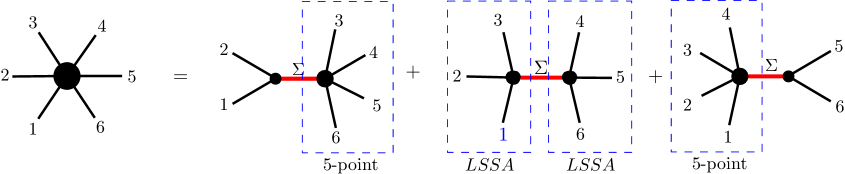
Figure 3: Expressing the 6-point KN amplitude in terms of the LSSA by the first recursion

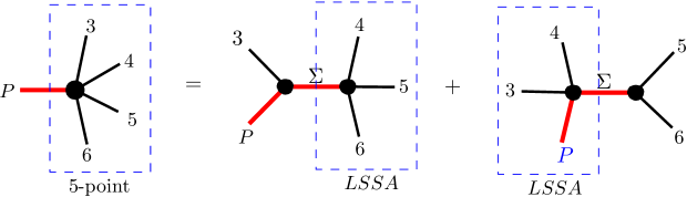
Figure 4: Expressing the 6-point KN amplitude in terms of the LSSA by the second recursion

On the other hand, the result of Eq.(3.35) tells us that the residue $R_{4,4}^{M}$ is a sum of products of the Lauricella functions after term by term integrations for a given $M$. We conclude that the $6$-point KN amplitude is a LSSA. It is interesting to note that to obtain the LSSA form of the residue $R_{4,4}^{M}$, one needs only do one-step recursion from the $6$-point KN amplitude. But to obtain the LSSA form of the residue $R_{3,5}^{M}$ ($R_{5,3}^{M}$), one needs to do $2$-step recursion or $(recursion)^{2}$. See Fig.3 and Fig.4.

In fact, to show that the $6$-point KN amplitude is a LSSA, one needs only do $1$-step recursion to express it in terms of the lower $5$-point and $4$-point amplitudes as was shown in Fig.3. Since we have shown that all $5$-point and $4$-point SSA are LSSA, the $6$-point KN amplitude is a LSSA. However, to explicitly calculate the LSSA form of the $6$-point KN amplitude, one needs to do the second recursion as was shown in Fig.4, and the calculation will be very lengthy.

The next step is to use the shifting principle to argue that all $6$-point SSA with arbitrary six tensor legs can be expressed in terms of the LSSA. The argument is obvious although the detailed calculation will again be very lengthy.

V.4 Seven-point SSA with tensor legs

For the case of $7$-point SSA, we first do $1$-step recursion on $7$-point KN amplitude. The subamplitude $R_{3,6}^{P,R}$ of the residue $R_{3,6}^{M}$ we obtained is the $6$-point SSA with five tachyons and one tensor leg. So for simplicity let’s first consider the five tachyons, one vector SSA ($\left(z_{1},z_{5},z_{6}\right)=\left(0,1,\infty\right)$)

$$A_{6}\left(\zeta_{1},k_{1};k_{2};k_{3};k_{4};k_{5};k_{6}\right)$$

$$=\int_{0}^{1}dz_{4}\int_{0}^{z_{4}}dz_{3}\int_{0}^{z_{3}}dz_{2}z_{2}^{k_{2}\cdot k_{1}}z_{3}^{k_{3}\cdot k_{1}}z_{4}^{k_{4}\cdot k_{1}}\left(1-z_{2}\right)^{k_{5}\cdot k_{2}}\left(1-z_{3}\right)^{k_{5}\cdot k_{3}}$$

$$\times\left(z_{4}-z_{2}\right)^{k_{4}\cdot k_{2}}\left(z_{4}-z_{3}\right)^{k_{4}\cdot k_{3}}\left(z_{3}-z_{2}\right)^{k_{3}\cdot k_{2}}$$

$$\times(-\zeta_{1})\cdot\left[\frac{k_{2}}{z_{2}}+\frac{k_{3}}{z_{3}}+\frac{k_{4}}{z_{4}}+\frac{k_{5}}{1}\right]$$

$$=A_{6}^{(1)}+A_{6}^{(2)}+A_{6}^{(3)}+A_{6}^{(4)}.$$ (5.69)

Mathematically, the calculation of all four terms in Eq.(5.69) are similar to the $6$-point KN amplitude which has been proved to be a LSSA in the last subsection. So the amplitude in Eq.(5.69) is a LSSA. According to the shifting principle, one can generalize the above calculation and consider five tachyons, one arbitrary tensor SSA and express them in terms of the LSSA. This proves that the residue $R_{3,6}^{M}$ of $7$-point KN amplitude is a LSSA. Similar consideration applies to the other residue $R_{6,3}^{M}$ of the $7$-point KN amplitude. The other two residues $R_{4,5}^{M}$, $R_{5,4}^{M}$ contain $5$-point and $4$-point SSA which have been shown to be LSSA. We conclude that the $7$-point KN amplitude is a LSSA. The next step is to use the shifting principle to argue that all $7$-point SSA with arbitrary seven tensor legs can be expressed in terms of the LSSA.

It is interesting to note that on the calculation of multi-step recursion processes, one encounters multi-tensor lower point SSA. For example, in addition to the $\zeta$ ($6$-point to $5$-point) in Eq.(5.23), there is another hidden leg in $R_{3,4}^{(1),M}$ ($R_{4,3}^{(1),M}$) when one performs the recursion from $5$-point to $4$-point. In sum, one obtains two tensor-legs in the final $4$-point LSSA when performing $2$-step recursion $(recursion)^{2}$ on the $6$-point KN amplitude. It is interesting to see that the multi-tensor SSA are associated with the multi-step recursion processes.

V.5 N-point SSA with tensor legs

In general, we can use mathematical induction, together with the on-shell recursion and the shifting principle, to show that all $n$-point SSA can be expressed in terms of the LSSA. The procedure goes as following. We assume that all $k$-point SSA ($k\leq n-1$) are LSSA, and we want to prove that all $n$-point SSA are LSSA. To prove this, we first apply the on-shell recursion to express the residue of $n$-point KN amplitude calculated in section III in terms of the lower point ($k\leq n-1$) SSA which were assumed to be LSSA. See Fig 1 above Eq.(3.27). So the $n$-point KN amplitude is a LSSA. We can then apply the shifting principle to show that all $n$-point SSA including the $n$-point KN amplitude are LSSA. This completes the proof.

As an example of application of the shifting principle, the $(n-1)$ tachyons, one vector SSA can be written as ($\left(z_{1},z_{n-1},z_{n}\right)=\left(0,1,\infty\right)$)

$$A_{n}\left(\zeta_{1},k_{1};k_{2};k_{3};k_{4};\cdot\cdot\cdot;k_{n}\right)$$

$$=\int_{0}^{1}dz_{n-2}\int_{0}^{z_{n-2}}dz_{n-3}\cdots\int_{0}^{z_{3}}dz_{2}\text{ }\prod_{i>j=1}^{n-2}\left(z_{i}-z_{j}\right)^{k_{i}\cdot k_{j}}$$

$$\times(-\zeta_{1})\cdot\left[\frac{k_{2}}{z_{2}}+\frac{k_{3}}{z_{3}}+\frac{k_{4}}{z_{4}}+\cdot\cdot\cdot+\frac{k_{n-1}}{1}\right]$$

$$=A_{n}^{(1)}+A_{n}^{(2)}+A_{n}^{(3)}+\cdot\cdot\cdot+A_{n}^{(n-2)}$$ (5.70)

where the calculation of each $A_{n}^{(j)}$ is similar to the $n$-point KN amplitude and can be expressed in terms of LSSA.

VI Conclusion

In this paper, we calculate explicitly residues of all $n$-point Koba-Nielsen (KN) amplitudes by using string on-shell recursion relation of string scattering amplitudes (SSA). We then use mathematical induction, together with the on-shell recursion and the shifting principle, to show that all $n$-point SSA including the KN amplitudes can be expressed in terms of the LSSA. In general, to explicitly calculate the LSSA form of the $n$-point KN amplitude, one needs to apply up to ($n-4)$-step recursion $(recursion)^{n-4}$ to achieve a $4$-point LSSA. These results demonstrates the exact $SL(K+3,\mathbb{C})$ symmetry of the tree-level open bosonic string theory.

Moreover, we derive an iteration relation among the residues of a given $n$-point KN amplitude. This iteration relation is a generalization of the case of simple Veneziano amplitude to the higher point SSA. We argue that this iteration relation is related to the $SL(K+3,\mathbb{C})$ symmetry and can presumably, in the $4$-point case, be used to soften the well-known hard Veneziano amplitude. So we expect the $SL(K+3,\mathbb{C})$ symmetry can be used to soften all higher $n$-point hard SSA. This mechanism is reminiscent of symmetry principle in QFT.

In the calculation of multi-tensor SSA, we discover that the calculation of SSA expressed in terms of the Lauricella functions is much simpler than the traditional calculation KLT . It is also interesting to see that to express the residues of higher point SSA in terms of the Lauricella $4$-point function, one encounters application of the multi-step recursion processes which are associated with the multi-tensor SSA calculation.

It will be important to extend the results of this paper to the superstring theory. However, the known construction of the string fermion vertex involved only the leading Regge trajectory fermion string state of the R sector PFSSA ; Osch ; RRR . It is a nontrivial task to construct the general massive fermion string vertex operators m1 ; m2 ; m3 ; m4 . Many questions related to the construction of SSA involving the general massive fermion string states need to be answered before one can further understand the symmetry of superstring theory.

In addition to the dynamics of $4$-point SSA with higher spin particles, there are many interesting issues related to higher point SSA. To name some, is there any evidence of the $SL(K+3,\mathbb{C})$ symmetry other than deriving it from SSA? In a recent publication LLYT , it was shown that the LSSA of three tachyons and one arbitrary string states can be rederived from the deformed cubic string field theory (SFT) Taejin . But can one use Witten SFT to obtain the $SL(K+3,\mathbb{C})$ symmetry ? How to deal with the $z_{4}\rightarrow\infty$ limit as was shown in Eq.(5.15) when calculating SSA with higher spin particles putting at $z_{4}$ ? Are there linear relations among higher point ($n\geq 5$) hard SSA similar to those of the $4$-point case? We hope to address these issues in the next publications.

Appendix A Generating function

In this appendix, we prove two relations which we used in the text to do the residue calculation. We begin with the generating function

$$e^{x\left[z+\frac{z^{2}}{2}+\frac{z^{3}}{3}+\cdots\right]}=e^{\left[xz+\frac{xz^{2}}{2}+\frac{xz^{3}}{3}+\cdots\right]}$$ (A.1)

which we used in Eq.(3.1) to do the residue calculation of the Veneziano amplitude. For our purpose here, let’s generalize this function and consider

$$A\left(x_{1},x_{2},\cdots;z\right) =\exp\left[B\left(x_{1},x_{2},\cdots;z\right)\right]=e^{\left[x_{1}z+\frac{x_{2}z^{2}}{2}+\frac{x_{3}z^{3}}{3}+\cdots\right]}$$

$$=\underset{m=0}{\overset{\infty}{\sum}}E_{m}\left(x_{1},x_{2},\cdots,x_{m}\right)z^{m}.$$ (A.2)

Two simple applications of the functions $E_{m}\left(x_{1},x_{2},\cdots,x_{m}\right)$ follow. If we set $x_{i}=x$ for all $i$, we obtain

$$A\left(x_{1},x_{2},\cdots;z\right)=\exp\left[x\left(z+\frac{z^{2}}{2}+\frac{z^{3}}{3}+\frac{z^{4}}{4}+\frac{z^{5}}{5}\cdots\right)\right]$$

$$=E_{0}+E_{1}\left(x\right)z+E_{2}\left(x\right)z^{2}+E_{3}\left(x\right)z^{3}+E_{4}\left(x\right)z^{4}+\cdots$$ (A.3)

with

$$E_{0} =1=\frac{\left(x\right)_{0}}{0!}$$

$$E_{1} =\frac{1}{1}x=x=\frac{x}{1!}=\frac{\left(x\right)_{1}}{1!}$$

$$E_{2} =\frac{1}{2}x+\frac{1}{2!}\left(\frac{1}{1}\right)^{2}x^{2}=\frac{x\left(x+1\right)}{2!}=\frac{\left(x\right)_{2}}{2!}$$

$$E_{3} =\frac{1}{3}x+\frac{1}{1!1!}\left(\frac{1}{2}\right)\left(\frac{1}{1}\right)x^{2}+\frac{1}{3!}\left(\frac{1}{1}\right)^{3}x^{3}=\frac{x\left(x+1\right)\left(x+2\right)}{3!}=\frac{\left(x\right)_{3}}{3!}$$

$$E_{4} =\frac{1}{4}x+\left[\frac{1}{1!1!}\left(\frac{1}{3}\right)\left(\frac{1}{1}\right)+\frac{1}{2!}\left(\frac{1}{2}\right)^{2}\right]x^{2}$$

$$+ \frac{1}{2!1!}\left(\frac{1}{1}\right)^{2}\left(\frac{1}{2}\right)x^{3}+\frac{1}{4!}\left(\frac{1}{1}\right)^{4}x^{4}=\frac{x\left(x+1\right)\left(x+2\right)\left(x+3\right)}{4!}=\frac{\left(x\right)_{4}}{4!}$$

$$\cdots$$ (A.4)

The coefficient functions above find application in Eq.(3.6) which corresponds to the residues of the Veneziano amplitude. On the other hand, if we set $\left(x_{1},x_{2},\cdots;z\right)=\left(\alpha_{-1},\alpha_{-2},\cdots;z\right)$, we obtain

$$A\left(\alpha_{-1},\alpha_{-2},\cdots;z\right)=\exp\left[\alpha_{-1}z+\frac{\alpha_{-2}z^{2}}{2}+\frac{\alpha_{-3}z^{3}}{3}+\frac{\alpha_{-4}z^{4}}{4}+\frac{\alpha_{-5}z^{5}}{5}\cdots\right]$$

$$=E_{0}+E_{1}\left(\alpha_{-1}\right)z+E_{2}\left(\alpha_{-1},\alpha_{-2}\right)z^{2}+E_{3}\left(\alpha_{-1},\alpha_{-2},\alpha_{-3}\right)z^{3}$$

$$+E_{4}\left(\alpha_{-1},\alpha_{-2},\alpha_{-3},\alpha_{-4}\right)z^{4}+...$$ (A.5)

with

$$E_{0} =1$$

$$E_{1} =\frac{\alpha_{-1}}{1}$$

$$E_{2} =\frac{\alpha_{-2}}{2}+\frac{1}{2!}\left(\frac{\alpha_{-1}}{1}\right)^{2}$$

$$E_{3} =\frac{\alpha_{-3}}{3}+\frac{1}{1!1!}\left(\frac{\alpha_{-2}}{2}\right)\left(\frac{\alpha_{-1}}{1}\right)+\frac{1}{3!}\left(\frac{\alpha_{-1}}{1}\right)^{3}$$

$$E_{4} =\frac{\alpha_{-4}}{4}+\frac{1}{1!1!}\left(\frac{\alpha_{-3}}{3}\right)\left(\frac{\alpha_{-1}}{1}\right)+\frac{1}{2!}\left(\frac{\alpha_{-2}}{2}\right)^{2}+\frac{1}{2!1!}\left(\frac{\alpha_{-1}}{1}\right)^{2}\left(\frac{\alpha_{-2}}{2}\right)+\frac{1}{4!}\left(\frac{\alpha_{-1}}{1}\right)^{4}$$

$$\cdots$$

$$E_{M} =\underset{\left\{N_{t}\right\},M=\underset{t=1}{\overset{\infty}{{\displaystyle\sum}}}tN_{t}}{\sum}\prod_{r=1}\frac{\left(\alpha_{-r}\right)^{N_{r}}}{N_{r}!r^{Nr}}$$ (A.6)

where in Eq.(A.6) the sum is over partitions of $N$ into $\left\{N_{r}\right\}$ with $M=\underset{r=1}{\sum}rN_{r}$ and $N=\underset{r=1}{\sum}N_{r}$. The coefficient $E_{M}$ above reminds us of the sum over normalized creation operators of the string spectrum at mass level $M$.

There are two relations which we used in the text to do the residue calculation. They are

$$F_{M}\left(x_{1},x_{2}\right) =\underset{b+c=M,b,c=0}{\sum}\frac{\left(T_{1}\right)_{b}}{b!}\frac{\left(T_{2}\right)_{c}}{c!}x_{1}^{b}x_{2}^{c}$$

$$=\underset{\left\{N_{r}\right\},M=\underset{r=1}{\sum}rN_{r}}{\sum}\prod_{r=1}\left(\frac{1}{N_{r}!r^{N_{r}}}\left[T_{1}x_{1}^{r}+T_{2}x_{2}^{r}\right]^{N_{r}}\right),$$ (A.7)

and the following recurrence relation

$$F_{M}\left(x_{1},x_{2}\right)=\underset{N=0}{\overset{M-1}{\sum}}F_{N}\left(x_{1},x_{2}\right)\left[T_{1}x_{1}^{M-N}+T_{2}x_{2}^{M-N}\right].$$ (A.8)

To prove Eq.(A.7), we introduce the generating function

$$G\left(x_{1},x_{2};z\right) =\left(1-zx_{1}\right)^{-T_{1}}\left(1-zx_{2}\right)^{-T_{2}}$$

$$=\underset{b,c=0}{\sum}\frac{\left(T_{1}\right)_{b}}{b!}\frac{\left(T_{2}\right)_{c}}{c!}x_{1}^{b}x_{2}^{c}z^{b+c},$$ (A.9)

and

$$F_{M}\left(x_{1},x_{2}\right) =\frac{1}{M!}\frac{\partial^{M}}{\partial z^{M}}G\left(x_{1},x_{2};z\right)|_{z=0}$$

$$=\underset{b+c=M,b,c=0}{\sum}\frac{\left(T_{1}\right)_{b}}{b!}\frac{\left(T_{2}\right)_{c}}{c!}x_{1}^{b}x_{2}^{c}.$$ (A.10)

On the other hand, we note that

$$G\left(x_{1},x_{2},z\right) =\left(1-zx_{1}\right)^{-T_{1}}\left(1-zx_{2}\right)^{-T_{2}}=\exp\left[-T_{1}\ln\left(1-zx_{1}\right)-T_{2}\ln\left(1-zx_{2}\right)\right]$$

$$=\exp\left[T_{1}\left(zx_{1}+\frac{\left(zx_{1}\right)^{2}}{2}+\frac{\left(zx_{1}\right)^{3}}{3}+\cdots\right)+T_{2}\left(zx_{2}+\frac{\left(zx_{2}\right)^{2}}{2}+\frac{\left(zx_{1}\right)^{3}}{3}+\cdots\right)\right]$$

$$=\exp\left[\left(T_{1}x_{1}+T_{2}x_{2}\right)z+\left(T_{1}x_{1}^{2}+T_{2}x_{2}^{2}\right)\frac{z^{2}}{2}+\left(T_{1}x_{1}^{3}+T_{2}x_{2}^{3}\right)\frac{z^{3}}{3}+\cdots\right]$$

$$=A\left(T_{1}x_{1}+T_{2}x_{2},T_{1}x_{1}^{2}+T_{2}x_{2}^{2},T_{1}x_{1}^{3}+T_{2}x_{2}^{3},\cdots;z\right),$$ (A.11)

so

$$F_{M}\left(x_{1},x_{2}\right) =E_{M}\left(T_{1}x_{1}+T_{2}x_{2},T_{1}x_{1}^{2}+T_{2}x_{2}^{2},\cdots,T_{1}x_{1}^{M}+T_{2}x_{2}^{M}\right)$$

$$=\sum_{\left\{N_{r}\right\}\text{,with }M=\underset{r}{\sum}rN_{r}}\prod_{r=1}\left(\frac{\left(T_{1}x_{1}^{r}+T_{2}x_{2}^{r}\right)^{N_{r}}}{N_{r}!r^{N_{r}}}\right)$$ (A.12)

where we have used Eq.(A.6) to obtain Eq.(A.12). This completes the proof of Eq.(A.7). It is straightforward to generalize Eq.(A.7) to

$$F_{M}\left(x_{1},\cdots,x_{n}\right) =\underset{\begin{array}[c]{c}a_{1}+\cdots+a_{n}=M\\ a_{1},\cdots,a_{n}=0\end{array}}{\sum}\frac{\left(T_{1}\right)_{a_{1}}}{a_{1}!}\cdots\frac{\left(T_{n}\right)_{a_{n}}}{a_{n}!}x_{1}^{a_{1}}\cdots x_{n}^{a_{n}}$$ (A.15)

$$=\underset{\left\{N_{r}\right\}\text{,with fixed }M=\underset{r}{\sum}rN_{r}}{\sum}\prod_{r=1}\left(\frac{1}{N_{r}!r^{N_{r}}}\left[T_{1}x_{1}^{r}+\cdots+T_{n}x_{n}^{r}\right]^{N_{r}}\right).$$ (A.16)

It can be shown that $E_{m}\left(x_{1},\cdots,x_{m}\right)$ satisfies a iteration relation

$$E_{m}\left(x_{1},\cdots,x_{m}\right) =\frac{1}{m!}\frac{\partial^{m}}{\partial z^{m}}A\left(x_{1},\cdots;z\right)|_{z=0}=\frac{1}{m!}\frac{\partial^{m-1}}{\partial z^{m-1}}\left(\frac{\partial B}{\partial z}e^{B}\right)|_{z=0}$$

$$=\frac{1}{m}\underset{n=0}{\overset{m-1}{\sum}}\frac{1}{n!}\left(\frac{\partial^{n}}{\partial z^{n}}e^{B}\right)\frac{1}{\left(m-n-1\right)!}\frac{\partial^{m-1-n}}{\partial z^{m-1-n}}\left(\frac{\partial B}{\partial z}\right)|_{z=0}$$

$$=\frac{1}{m}\underset{n=0}{\overset{m-1}{\sum}}\frac{1}{n!}\left(\frac{\partial^{n}}{\partial z^{n}}e^{B}\right)|_{z=0}\left[x_{m-n}+O\left(z\right)\right]|_{z=0}=\frac{1}{m}\underset{n=0}{\overset{m-1}{\sum}}E_{n}\left(x_{1},\cdots,x_{n}\right)x_{m-n}.$$ (A.17)

If we put $x_{i}=\alpha_{-i}$ for all $i$, we obtain

$$E_{m}\left(\alpha_{-1},\alpha_{-2},\cdots;\alpha_{-m}\right)=\frac{1}{m}\underset{n=1}{\overset{m-1}{\sum}}E_{n}\left(\alpha_{-1},\alpha_{-2},\cdots;\alpha_{-n}\right)\alpha_{-\left(m-n\right)}.$$ (A.18)

Similarly, $F_{M}\left(x_{1},x_{2}\right)$ obeys a iteration relation

$$F_{M}\left(x_{1},x_{2}\right)=\frac{1}{M!}\frac{\partial^{M}}{\partial z^{M}}G\left(x_{1},x_{2};z\right)|_{z=0}$$

$$=\frac{1}{M!}\frac{\partial^{M}}{\partial z^{M}}\left(1-zx_{1}\right)^{-T_{1}}\left(1-zx_{2}\right)^{-T_{2}}|_{z=0}$$

$$=\frac{1}{M!}\frac{\partial^{M-1}}{\partial z^{M-1}}\left[\left(1-zx_{1}\right)^{-T_{1}}\left(1-zx_{2}\right)^{-T_{2}}\left(\frac{x_{1}T_{1}}{1-zx_{1}}+\frac{x_{1}T_{2}}{1-zx_{2}}\right)\right]|_{z=0},$$ (A.19)

which can be written as

$$=\frac{1}{M!}\underset{N=0}{\overset{M-1}{\sum}}\left[\begin{array}[c]{c}\frac{\left(M-1\right)!}{N!\left(M-1-N\right)!}\frac{\partial^{N}}{\partial z^{N}}\left(\left(1-zx_{1}\right)^{-T_{1}}\left(1-zx_{2}\right)^{-T_{2}}\right)|_{z=0}\\ \times\frac{\partial^{M-1-N}}{\partial z^{M-1-N}}\left(\frac{x_{1}T_{1}}{1-zx_{1}}+\frac{x_{1}T_{2}}{1-zx_{2}}\right)|_{z=0}\end{array}\right]$$ (A.22)

$$=\frac{1}{M}\underset{N=0}{\overset{M-1}{\sum}}\frac{1}{N!}\frac{\partial^{N}}{\partial z^{N}}\left(\left(1-zx_{1}\right)^{-T_{1}}\left(1-zx_{2}\right)^{-T_{2}}\right)|_{z=0}\left(T_{1}x_{1}^{M-N}+T_{2}x_{2}^{M-N}\right)$$

$$=\frac{1}{M}\underset{N=0}{\overset{M-1}{\sum}}F_{N}\left(x_{1},x_{2}\right)\left(T_{1}x_{1}^{M-N}+T_{2}x_{2}^{M-N}\right).$$ (A.23)

This completes the proof of Eq.(A.8). It is straightforward to generalize Eq.(A.8) to

$$F_{M}\left(x_{1},x_{2},\cdots,x_{n}\right)=\underset{N=0}{\overset{M-1}{\sum}}F_{N}\left(x_{1},x_{2},\cdots,x_{n}\right)\left[T_{1}x_{1}^{M-N}+T_{2}x_{2}^{M-N}+\cdots+T_{n}x_{n}^{M-N}\right].$$ (A.24)

References

- (1) MB Green, JH Schwarz and E Witten. Superstring theory, v. 1. Cambridge University,Cambridge, (1987).
- (2) Gregory Moore. Finite in all directions. arXiv preprint hep-th/9305139, 1993.
- (3) Gregory Moore. Symmetries of the bosonic string S-matrix. arXiv preprint hep-th/9310026, 1993.
- (4) Chuan-Tsung Chan, Shoichi Kawamoto, and Dan Tomino. To see symmetry in a forest of trees. Nucl. Phys. B, 885:225–265, 2014.
- (5) Sheng-Hong Lai, Jen-Chi Lee, and Yi Yang. The lauricella functions and exact string scattering amplitudes. Journal of High Energy Physics, 2016(11):62, 2016.
- (6) S. H. Lai, J. C. Lee and Yi Yang, ”The Symmetry of the Bosonic String Scattering Amplitudes”, Nucl. Phys. B 941 (2019) 53-71.
- (7) Willard Miller Jr. Symmetry and separation of variables. Addison-Wesley, Reading, Massachusetts, 1977.
- (8) S. H. Lai, J. C. Lee and Yi Yang, ”Solving Lauricella String Scattering Amplitudes through recurrence relations”, JHEP 09 (2017) 130.
- (9) S. H. Lai, J. C. Lee and Yi Yang, ”Recent developments of the Lauricella string scattering amplitudes and their exact Symmetry”, Symmetry 13 (2021) 454, arXiv:2012.14726 [hep-th].
- (10) Steven B Giddings, David J Gross, and Anshuman Maharana. Gravitational effects in ultrahigh-energy string scattering. Physical Review D, 77(4):046001, 2008.
- (11) Daniele Amati, M Ciafaloni, and G Veneziano. Superstring collisions at Planckian energies. Phys. Lett. B, 197(1):81–88, 1987.
- (12) Daniele Amati, M Ciafaloni, and G Veneziano. Classical and quantum gravity effects from Planckian energy superstring collisions. Int. J. of Mod. Phys. A, 3(07):1615–1661, 1988.
- (13) Daniele Amati, Marcello Ciafaloni, and Gabriele Veneziano. Can spacetime be probed below the string size? Phys. Lett. B, 216(1):41–47, 1989.
- (14) M Soldate. Partial-wave unitarity and closed-string amplitudes. Phys. Lett. B, 186(3):321–327, 1987.
- (15) IJ Muzinich and M Soldate. High-energy unitarity of gravitation and strings. Phys. Rev. D, 37(2):359, 1988.
- (16) Richard C Brower, Joseph Polchinski, Matthew J Strassler, and Chung-I Tan. The Pomeron and gauge/string duality. JHEP, 2007(12):005, 2007.
- (17) Richard C Brower, Horatiu Nastase, Howard J Schnitzer, and Chung-I Tan. Analyticity for multi-Regge limits of the Bern–Dixon–Smirnov amplitudes. Nucl. Phys. B, 822(1):301–347, 2009.
- (18) David J Gross and Paul F Mende. The high-energy behavior of string scattering amplitudes. Phys. Lett. B, 197(1):129–134, 1987.
- (19) David J Gross and Paul F Mende. String theory beyond the Planck scale. Nucl. Phys. B, 303(3):407–454, 1988.
- (20) David J Gross and JL Manes. The high energy behavior of open string scattering. Nucl. Phys. B, 326(1):73–107, 1989.
- (21) David J. Gross. High-Energy Symmetries of String Theory. Phys. Rev. Lett., 60:1229, 1988.
- (22) D. J. Gross. Strings at superPlanckian energies: In search of the string symmetry. In In *London 1988, Proceedings, Physics and mathematics of strings* 83-95. (Philos. Trans. R. Soc. London A329 (1989) 401-413)., 1988.
- (23) Chuan-Tsung Chan and Jen-Chi Lee. Stringy symmetries and their high-energy limits. Phys. Lett. B, 611(1):193–198, 2005.
- (24) Chuan-Tsung Chan and Jen-Chi Lee. Zero-norm states and high-energy symmetries of string theory. Nucl. Phys. B, 690(1):3–20, 2004.
- (25) Chuan-Tsung Chan, Pei-Ming Ho, and Jen-Chi Lee. Ward identities and high energy scattering amplitudes in string theory. Nucl. Phys. B, 708(1):99–114, 2005.
- (26) Chuan-Tsung Chan, Pei-Ming Ho, Jen-Chi Lee, Shunsuke Teraguchi, and Yi Yang. High-energy zero-norm states and symmetries of string theory. Phys. Rev. Lett., 96(17):171601, 2006.
- (27) Chuan-Tsung Chan, Pei-Ming Ho, Jen-Chi Lee, Shunsuke Teraguchi, and Yi Yang. Solving all 4-point correlation functions for bosonic open string theory in the high-energy limit. Nucl. Phys. B, 725(1):352–382, 2005.
- (28) Jen-Chi Lee. New symmetries of higher spin states in string theory. Physics Letters B, 241(3):336–342, 1990.
- (29) Jen-Chi Lee and Burt A Ovrut. Zero-norm states and enlarged gauge symmetries of the closed bosonic string with massive background fields. Nucl. Phys. B, 336(2):222–244, 1990.
- (30) Jen-Chi Lee. Decoupling of degenerate positive-norm states in string theory. Phys. Rev. Lett., 64(14):1636, 1990.
- (31) Jen-Chi Lee and Yi Yang. Review on high energy string scattering amplitudes and symmetries of string theory. arXiv preprint arXiv:1510.03297, 2015.
- (32) Jen-Chi Lee and Yi Yang. Overview of high energy string scattering amplitudes and symmetries of string theory. Symmetry, 11(8):1045, 2019.
- (33) Bagchi, Arjun, Aritra Banerjee, and Shankhadeep Chakrabortty. ”Rindler Physics on the String Worldsheet.” Physical Review Letters 126.3 (2021): 031601.
- (34) Eberhardt, Lorenz. ”Partition functions of the tensionless string.” arXiv preprint arXiv:2008.07533 (2020).
- (35) Bagchi, Arjun, et al. ”A tale of three—tensionless strings and vacuum structure.” Journal of High Energy Physics 2020.4 (2020): 1-53.
- (36) Lee, Seung-Joo, Wolfgang Lerche, and Timo Weigand. ”Tensionless strings and the weak gravity conjecture.” Journal of High Energy Physics 2018.10 (2018): 1-83.
- (37) Bagchi, Arjun, et al. ”Inhomogeneous tensionless superstrings.” Journal of High Energy Physics 2018.2 (2018): 1-33.
- (38) Yu, Ming, Chi Zhang, and Yao-Zhong Zhang. ”One loop amplitude from null string.” Journal of High Energy Physics 2017.6 (2017): 1-18.
- (39) Hohm, Olaf, Usman Naseer, and Barton Zwiebach. ”On the curious spectrum of duality invariant higher-derivative gravity.” Journal of High Energy Physics 2016.8 (2016): 1-31.
- (40) Bagchi, Arjun, Shankhadeep Chakrabortty, and Pulastya Parekh. ”Tensionless superstrings: view from the worldsheet.” Journal of High Energy Physics 2016.10 (2016): 1-24.
- (41) Bagchi, Arjun, Shankhadeep Chakrabortty, and Pulastya Parekh. ”Tensionless strings from worldsheet symmetries.” Journal of High Energy Physics 2016.1 (2016): 158.
- (42) Gaberdiel, Matthias R., and Rajesh Gopakumar. ”Higher spins & strings.” Journal of High Energy Physics 2014.11 (2014): 44.
- (43) Sagnotti, A., and M. Tsulaia. ”On higher spins and the tensionless limit of string theory.” Nuclear Physics B 682.1-2 (2004): 83-116.
- (44) Yung-Yeh Chang, Bo Feng, Chih-Hao Fu, Jen-Chi Lee,Yihong Wang and Yi Yang, ”A note on on-shell recursion relation of string amplitudes”, JHEP 02 (2013) 028.
- (45) R. H. Boels, D. Marmiroli and N. A. Obers, “On-shell Recursion in String Theory,” JHEP 1010 (2010) 034 [arXiv:1002.5029 [hep-th]].
- (46) C. Cheung, D. O’Connell and B. Wecht, “BCFW Recursion Relations and String Theory,” JHEP 1009 (2010) 052 [arXiv:1002.4674 [hep-th]].
- (47) R. Britto, F. Cachazo and B. Feng, “New recursion relations for tree amplitudes of gluons,” Nucl. Phys. B 715 (2005) 499 [hep-th/0412308].
- (48) R. Britto, F. Cachazo, B. Feng and E. Witten, “Direct proof of tree-level recursion relation in Yang-Mills theory,” Phys. Rev. Lett. 94 (2005) 181602 [hep-th/0501052].
- (49) Sheng-Hong Lai, Jen-Chi Lee, Taejin Lee and Yi Yang, Phys. Lett. B 776 (2018) 150-157.
- (50) Taejin Lee, Phys. Lett. B 768 (2017) 248.
- (51) J AppellPandKampé de Fériet. Fonctions hypergéométriques et hypersphériques, 1926.
- (52) Ko, S.-L.; Lee, J.-C.; Yang, Y. Patterns of high energy massive string scatterings in the regge regime. J. High Energy Phys. 2009, 2009, 28.
- (53) Lee, J.-C.; Yan, C.H.; Yang, Y. High-energy string scattering amplitudes and signless Stirling number identity. SIGMA Symmetry Integr. Geom. Methods Appl. 2012, 8, 45.
- (54) H. Kawai, David C Lewellen, and S-HH Tye. A relation between tree amplitudes of closed and open strings. Nucl. Phys. B, 269(1):1–23, 1986.
- (55) Sheng-Hong Lai, Jen-Chi Lee, and Yi Yang, work in progress.
- (56) S. H. Lai, J. C. Lee and Yi Yang, Phys. Lett. B797, 134812 (2019).
- (57) O. Schlotterer, ”Scattering amplitudes in open superstring theory”, Fortschr. Phys.60,No.5, 373-691 (2012).
- (58) I.G. Koh, W. Troost and A. Van Proeyen, Nucl. Phys. B292, 201 (1987).
- (59) M. Bianchi, L. Lopez, and R. Richter, ”On stable higher spin states in Heterotic String Theories,” JHEP 1103 (2011) 051
- (60) A. Hanany, D. Forcella, and J. Troost, ”The Covariant perturbative string spectrum”, Nucl.Phys. B846 (2011) 212.
- (61) Wan-Zhe Feng, Dieter Lust, Oliver Schlotterer, Stephan Stieberger, Tomasz R. Taylor, Nucl.Phys.B843, 570 (2011).
- (62) M. Vasiliev, ”Nonlinear equations for symmetric massless higher spin fields in (A)dS(d)”, Phys.Lett. B567 (2003) 139.