Instabilities of vortex-ring-bright soliton in trapped binary 3D Bose-Einstein condensates

Abstract

Instabilities of vortex-ring-bright coherent structures in harmonically trapped two-component three-dimensional Bose-Einstein condensates are studied numerically within the coupled Gross-Pitaevskii equations and interpreted analytically. Interestingly, the filled vortex core with a sufficiently large amount of the bright component is observed to reduce the parametric interval of stability of the vortex ring. We have identified the mechanisms of several linear instabilities and one nonlinear parametric instability in this connection. Two of the linear instabilities are qualitatively different from ones reported earlier, to our knowledge, and are associated with azimuthal modes of $m=0$ and $m=1$, i.e., deviations of the vortex from the stationary ring shape. Our nonlinear parametric resonance instability occurs between the $m=0$ and $m=2$ modes and signals the exchange of energy between them.

I Introduction

The study of Bose-Einstein condensates (BECs) has offered for two and a half decades now an ideal playground for the exploration of nonlinear phenomena Pethick and Smith (2002); Stringari and Pitaevskii (2003); Kevrekidis et al. (2015). Specifically, the study of topological excitations has been of wide interest to the research communities of atomic, nonlinear and wave physics Fetter and Svidzinsky (2001); Fetter (2009). Indeed, relevant reviews have focused not only on two-dimensional vortical structures, but also on three-dimensional vortex lines and vortex rings Komineas (2007), as well as on more complex patterns including skyrmions Marzlin et al. (2000); Mizushima et al. (2002); Reijnders et al. (2004), Dirac monopoles Ollikainen et al. (2017) and quantum knots Hall et al. (2016); Lee et al. (2018); Ruban (2018a); Ticknor et al. (2019).

While the majority of the studies has naturally been directed at the understanding of the single-component BEC setting, the study of multi-component BECs has also attracted considerable attention both in the two-component setting Kevrekidis and Frantzeskakis (2016), but also in the case of the so-called spinor condensates Kawaguchi and Ueda (2012); Stamper-Kurn and Ueda (2013) of more than two components. Indeed, such multi-component settings have offered an ideal framework for the exploration of ideas of phase separation Trippenbach et al. (2000); Barankov (2002); Lee et al. (2016); Indekeu et al. (2015), but also for the manifestation of a wide range of fluid-like instabilities. The latter include, among others, the Rayleigh-Taylor instability Sasaki et al. (2009); Gautam and Angom (2010); Kadokura et al. (2012), the Kelvin-Helmholtz instability Takeuchi et al. (2010a); Suzuki et al. (2010); Baggaley and Parker (2018), the capillary Sasaki et al. (2011); Indekeu et al. (2018) and Richtmyer-Meshkov Bezett et al. (2010) instabilities, as well as the countersuperflow Law et al. (2001); Yukalov and Yukalova (2004); Takeuchi et al. (2010b); Hamner et al. (2011), but also the Rosensweig Saito et al. (2009) instabilities. This wealth of findings clearly illustrates the fact that multi-component systems may possess a significant additional wealth of features, in comparison with the simpler single-component ones.

It is exactly on this nexus of nonlinear topological coherent structures and their instabilities, but focusing on the multi-component variants thereof that our present study intends to focus. Earlier work of different subsets of the present authors Bisset et al. (2015a); Wang et al. (2017); Bisset et al. (2015b); Ruban (2017a) has explored the instabilities of chiefly one-component, three-dimensional structures, such as vortex lines and vortex rings, as well as multi-line/ring variants thereof. The last few years have led to a deeper and intensified consideration of vortical patterns bearing a second component that fills the relevant vortex core Law et al. (2010); Pola et al. (2012); Hayashi et al. (2013), as well as their dynamics and instabilities Ruban (2021a, b), and interactions with each other Richaud et al. (2020, 2021) and with defects Wang (2021). Most of these above studies have been centered around the somewhat less computationally intensive, yet still quite interesting 2d realm. Our aim here is to extend such multi-component, filled-vortex considerations to structures arising in three-dimensional condensates. More concretely, as our prototypical example, we will explore filled-core vortex rings.

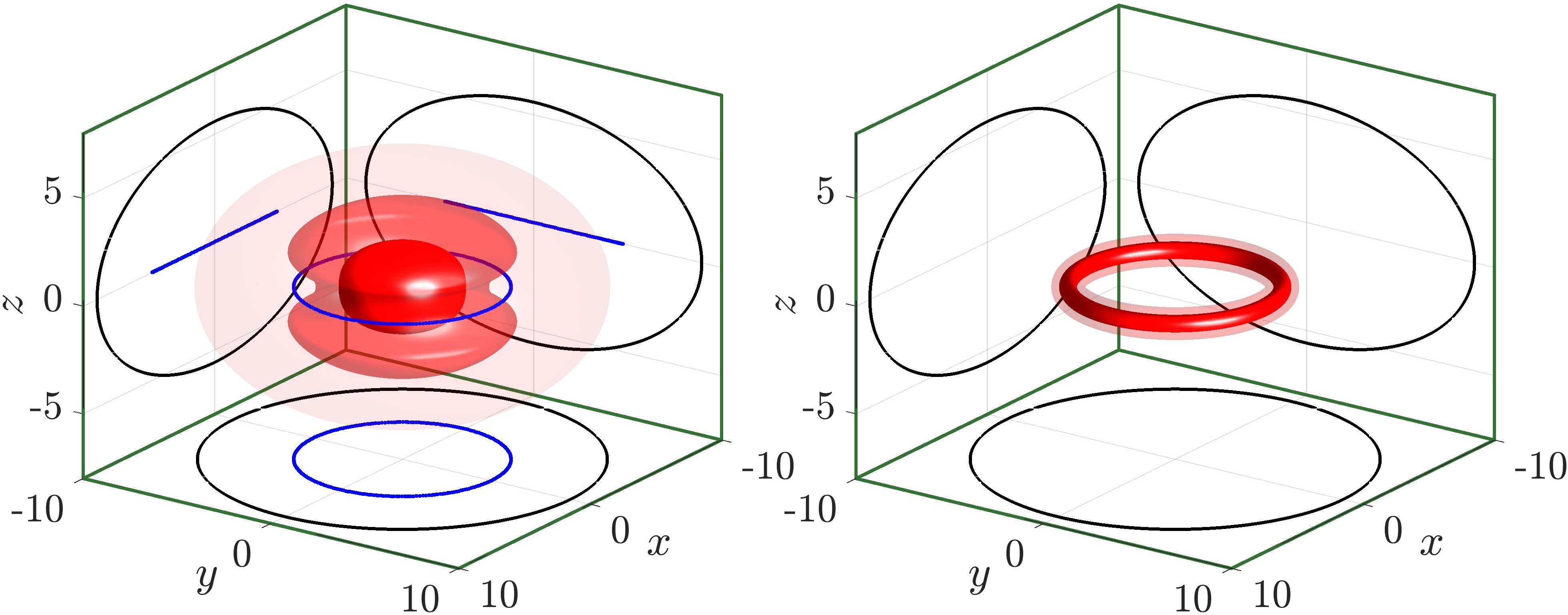
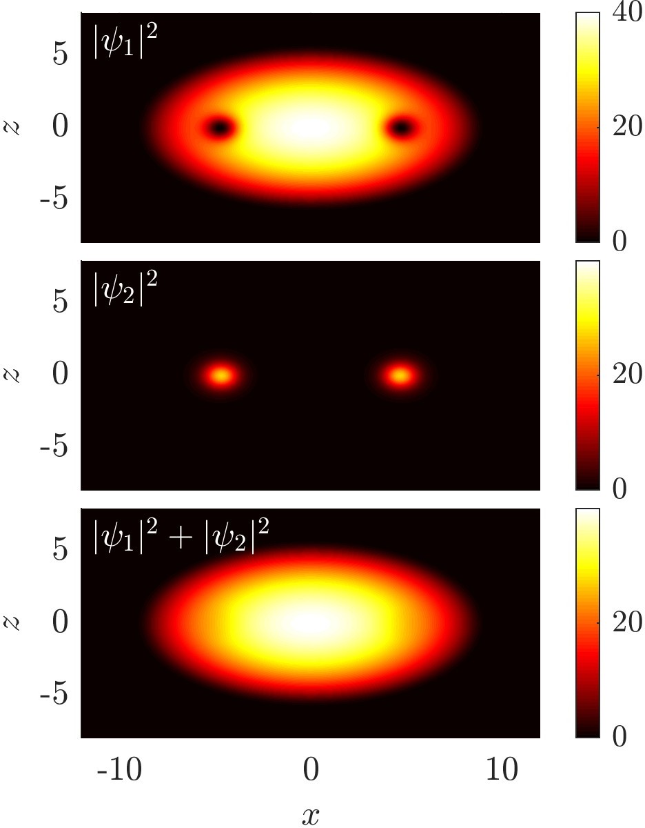
Figure 1: A typical, numerically exact fat-core VRB configuration with a relatively massive bright component at $\kappa=1.6,g_{12}=1.02,\mu_{1}=40$ and $\mu_{2}=39.6$. In the top row, the density contours are shown with the core of the VR highlighted in blue; the density projections along the different planes are also shown. In the second-fourth row panels, the density projections along the $x$-$z$ plane are illustrated in detail. Note that the configuration is rotationally symmetric about the $z$-axis. The vortical (dipolar) pattern of the second row and the bright (second component) pattern of the third row add up to the total density featuring a Thomas-Fermi (TF) profile for the density equal to $\max(\mu_{1}-V,0)$ on the fourth panel.

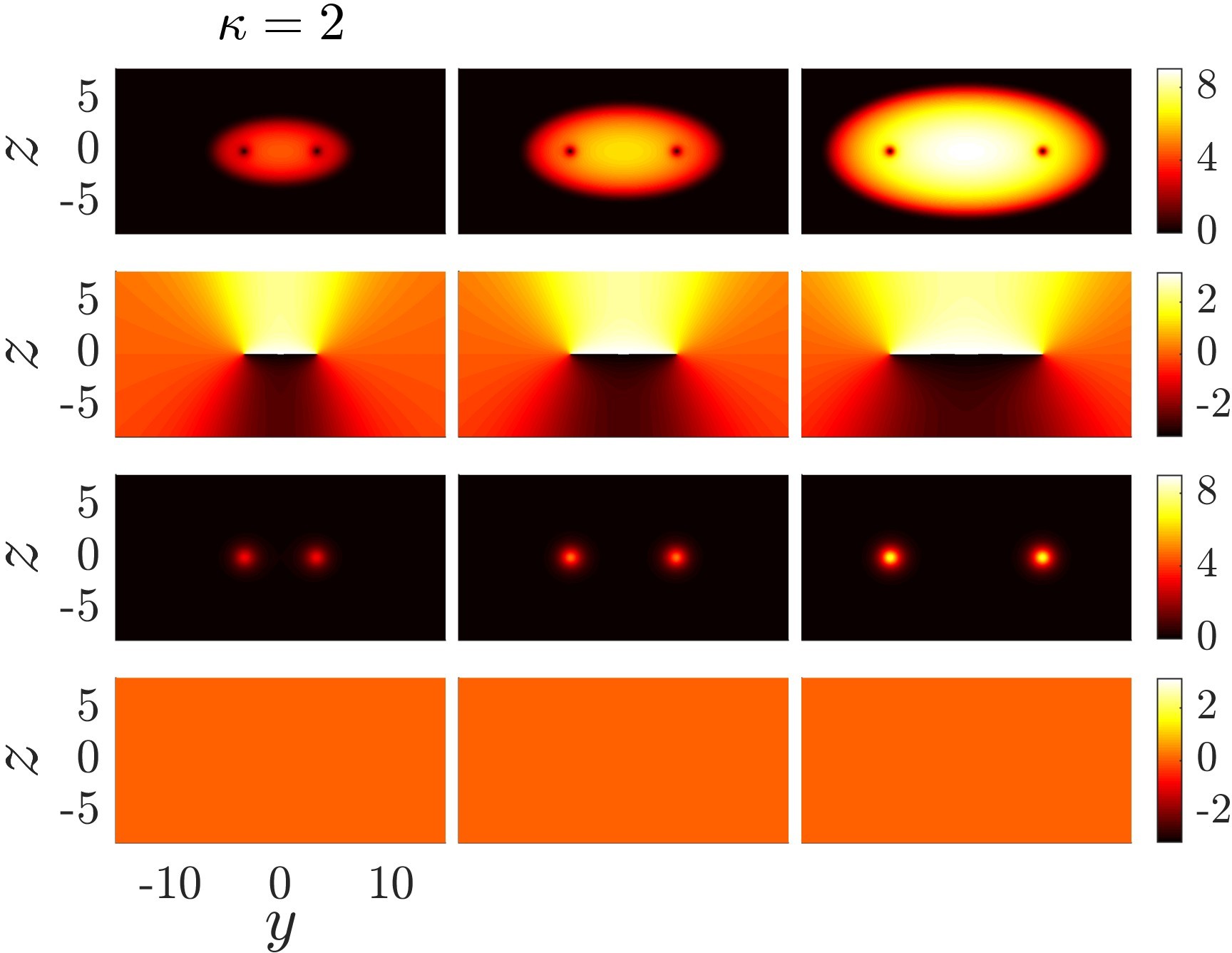
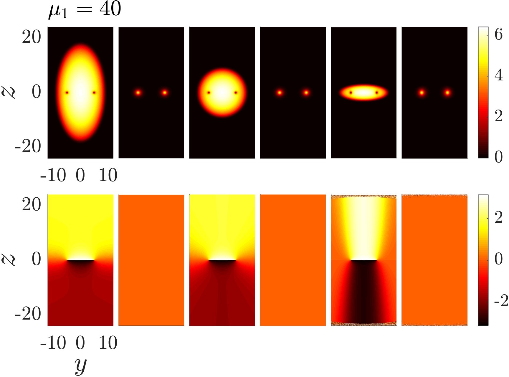
Figure 2: Typical stationary VRB configurations: the amplitude and phase profiles are depicted in odd and even rows, respectively. In top panels, the three columns, in turn, are for chemical potentials $\mu_{1}=20,40$ and $80$ at $\kappa=2$, see Eq. (43) for the respective values of $\mu_{2}$. In the bottom panels, the state at $\mu_{1}=40$ above is continued in the aspect ratio to $\kappa=0.5,1$ and $3$, respectively.

The so-called vortex-ring-bright (VRB) structures (see some numerical examples in Figs. 1 and 2) are among the canonical generalizations of the widely studied single-component vortex ring Komineas (2007); Wang et al. (2017); Ruban (2017a). For the latter in our earlier work, we had explored Ticknor et al. (2018) numerically the theoretically predicted instabilities Horng et al. (2006), finding that azimuthal perturbations of different modes of azimuthal wavenumber $m$ become unstable in different regimes of anisotropy of the condensate confinement. Indeed, for prolate BECs, the mode with $m=1$ was found to be unstable leading to tumbling motion of the VR structure. Weakly oblate BECs represented the canonical regions of stability of the VR, while sufficiently oblate ones led to the instability, progressively of the $m=2$, $m=3$ etc. modes, splitting the VR into two-, three- etc. vortex lines, respectively. Here, our aim is to examine what happens to the same phenomenology, when the core of the ring vortex is filled by a second component. In line with the wealth of phenomenology identified in earlier multi-component studies, we find a variety of potential instabilities, including some that are unprecedented, to the best of our knowledge. The $m=2$ mode instability still occurs, but at a wider range of anisotropies due to the presence of the second component. For the $m=1$ mode, an oscillatory variant of the relevant instability is newly emergent for a suitable range of atom numbers/chemical potentials. Finally, as concerns linear instabilities, in a narrow parametric regime an unprecedented instability of the $m=0$ mode is found to arise. Lastly, we also identify a nonlinear (parametric) instability stemming from the resonance between the $m=0$ and the $m=2$ modes, causing the exchange of energy between the two.

In what follows, our presentation of these phenomena for the VRB structures is as follows. First, we qualitatively justify theoretically the origin of these instabilities, after having presented the mathematical setup of our work. Then we present our computational setup, and in Sec. IV, we support our theoretical analysis by means of numerical computations of existence, stability and dynamics of VRB structures in different parametric regimes. Finally, in Sec. V, we summarize our findings and present our conclusions.

II Mathematical Setup & Qualitative Theoretical Analysis

II.1 The basic model

As the basic mathematical model for our setup, we employ the widely recognized coupled Gross-Pitaevskii equations for two complex wave functions, $\psi_{1}({\bf r},t)$ (the vortical component), and $\psi_{2}({\bf r},t)$ (the bright component) Pethick and Smith (2002); Stringari and Pitaevskii (2003); Kevrekidis et al. (2015). For simplicity, equal masses $m_{1}=m_{2}=m$ of the species atoms are considered. Let an axisymmetric harmonic trap be characterized by a perpendicular frequency $\omega_{\perp}$ and by an anisotropy $\kappa=\omega_{\parallel}/\omega_{\perp}$. Using the trap units $\tau=1/\omega_{\perp}$ for the time, $l_{\rm trap}=\sqrt{\hbar/(m\omega_{\perp})}$ for the length, and $\varepsilon=\hbar\omega_{\perp}$ for the energy, the equations of motion are written in dimensionless form

$${\sf i}\dot{\psi}_{1}=-\frac{1}{2}\nabla^{2}\psi_{1}+\left[V({\bf r})+g_{11}|\psi_{1}|^{2}+g_{12}|\psi_{2}|^{2}\right]\psi_{1},$$ (1)

$${\sf i}\dot{\psi}_{2}=-\frac{1}{2}\nabla^{2}\psi_{2}+\left[V({\bf r})+g_{21}|\psi_{1}|^{2}+g_{22}|\psi_{2}|^{2}\right]\psi_{2},$$ (2)

where the overdot stands for the temporal partial derivative,

$$V({\bf r})=(x^{2}+y^{2}+\kappa^{2}z^{2})/2$$ (3)

is the trap potential, while $g_{ij}$ is a symmetric $2\times 2$ matrix of nonlinear interactions. Physically, the interactions are determined by the scattering lengths $a_{ij}$ Pu and Bigelow (1998):

$$g^{\rm phys}_{ij}=2\pi\hbar^{2}a_{ij}(m_{i}^{-1}+m_{j}^{-1}),\qquad i,j=1,2.$$ (4)

In this work, we consider the symmetric case $a_{11}=a_{22}=a>0$, so the self-repulsion coefficients are equal to each other. It should be noted that while the setting, e.g., of ⁸⁷Rb features slight differences between the $a_{ij}$’s Egorov et al. (2013), it is possible to experimentally engineer the well-known, so-called Manakov case of equal interactions Lannig et al. (2020). Without loss of generality, the relevant coefficients can be normalized to the unit value, $g_{11}=g_{22}=1$. With this choice, the (conserved) numbers of trapped atoms are given by the relations

$$N_{1}=\frac{l_{\rm trap}}{4\pi a}\int|\psi_{1}|^{2}d^{3}{\bf r}=(l_{\rm trap}/a)n_{1},$$ (5)

$$N_{2}=\frac{l_{\rm trap}}{4\pi a}\int|\psi_{2}|^{2}d^{3}{\bf r}=(l_{\rm trap}/a)n_{2}.$$ (6)

In real experiments the ratio $l_{\rm trap}/a$ ranges typically from a few hundreds to a few thousands. In what follows, $n_{1}$ and $n_{2}$ will be important control parameters. The cross-repulsion coefficient will be assumed as $g_{12}=1+g$, with a small positive parameter $g$. The condition $g>0$ is required for the phase separation regime to take place Timmermans (1998); Ao and Chui (1998), as has also been experimentally manifested in Papp et al. (2008).

Since we intend to consider soft excitations on a stationary background, two more parameters will be used as well, namely the chemical potentials $\mu_{1}$ and $\mu_{2}$. The numbers of particles $n_{1}$ and $n_{2}$ are dependent upon $\mu_{1}$ and $\mu_{2}$. We are mainly interested in the Thomas-Fermi (TF) regime $\mu_{1}\gg 1$, when the (single component) background density profile is given by a simple approximate formula

$$|\psi_{1}^{(0)}|^{2}=\rho({\bf r})\approx\mu_{1}-V({\bf r}).$$ (7)

The typical sizes of the trapped cloud are thus $R_{\perp}=\sqrt{2\mu_{1}}$ and $R_{z}=R_{\perp}/\kappa$, while a typical width of an empty vortex core is $\xi_{*}\sim 1/\sqrt{\mu_{1}}$. Importantly, a filled vortex core can have a width $w$ which is essentially larger than $\xi_{*}$. Roughly $w$ can be estimated as

$$w\sim n_{2}^{1/2}\mu_{1}^{-3/4},$$ (8)

since an effective volume of the bright component is $\sim w^{2}\sqrt{\mu_{1}}$ (assuming a bright component that completely fills the vortex density dip; such a regime with $\mu_{1}\approx\mu_{2}$ is typical for the critical phenomena under consideration; see Fig. 1 for example), while a typical density of the bright component is $\sim\mu_{1}$. The inequality $w>\xi_{*}$ can be the reason for instability of a certain kind, as we will see further.

However, it is relevant to keep in mind that the VRB solutions may exist for a wide range of $\mu_{2}$ and not just for $\mu_{2}$ comparable to $\mu_{1}$. A good example to draw analogies with is the dark-bright solitons of Busch and Anglin (2001) where the analytical solution makes it clear that roughly the solutions exist for a very broad range of $\mu_{2}<\mu_{1}$.

II.2 Variational approach and approximate Hamiltonian

In the Thomas-Fermi regime, a typical time period for vortex motion is parametrically long, $\tau_{\rm vort}\sim\mu$, since the quantum of circulation is $2\pi\sim R_{\perp}^{2}/\tau_{\rm vort}$. On the other hand, typical periods of potential oscillations (sound modes) are about 1 and larger. Thus, the latter hard degrees of freedom are well separated from the soft degrees of freedom. As sound modes are not excited (sitting at much higher frequencies in the TF limit), the dynamics of soft modes can be described self-consistently through an appropriate effective vortex Lagrangian Ruban (2001). Here we briefly discuss some basic properties of such a variational description.

Let us first recall that the commonly used inertia-free approximation for a long-scale dynamics of a closed vortex filament in a trapped single-component BEC corresponds to a Lagrangian functional of the general form Ruban (2001, 2017a, 2018b)

$${\cal L}=\Gamma\oint{\bf F}({\bf R})\cdot[{\bf R}_{\beta}\times{\bf R}_{t}]d\beta-{\cal H}_{v}\{{\bf R}(\beta,t)\},$$ (9)

where $\Gamma=2\pi\hbar/m$ is the circulation quantum, and the unknown vector function ${\bf R}(\beta,t)$ describes the shape of the vortex in three dimensions, with $\beta$ being an arbitrary longitudinal parameter along the line. Here, the Hamiltonian ${\cal H}_{v}$ is the vortex energy on the given density background. For self-consistency, the vector function ${\bf F}({\bf R})$ should satisfy the condition Ruban (2017a)

$$\mbox{div}_{\bf R}{\bf F}({\bf R})=\rho({\bf R}).$$ (10)

The equation of motion in the vector form reads

$$\Gamma[{\bf R}_{\beta}\times{\bf R}_{t}]\rho({\bf R})=\delta{\cal H}_{v}/\delta{\bf R}.$$ (11)

If the shape of the distorted vortex ring is given in the cylindrical coordinates by two real functions $R(\varphi,t)$ and $Z(\varphi,t)$ characterizing the radial extent of the VR and its $z$-location, then the two scalar equations of motion are of the following non-canonical Hamiltonian form,

$$\Gamma\rho(R,Z)R\dot{Z} = \delta{\cal H}_{v}/\delta R,$$ (12)

$$-\Gamma\rho(R,Z)R\dot{R} = \delta{\cal H}_{v}/\delta Z.$$ (13)

For configurations such as a moderately perturbed vortex ring, the vortex Hamiltonian ${\cal H}_{v}$ is often taken in the Local Induction Approximation (LIA), which corresponds to the deep TF regime Ruban (2001):

$${\cal H}_{v} \approx {\cal H}_{\rm LIA}=\frac{\Gamma^{2}}{4\pi}\Lambda\oint\rho({\bf R})|{\bf R}_{\beta}|d\beta$$ (14)

$$= \frac{\Gamma^{2}}{4\pi}\Lambda\int\rho(R,Z)\sqrt{R^{2}+R^{\prime 2}+Z^{\prime 2}}d\varphi,$$

where $\Lambda=\ln(R_{*}/\xi_{*})\approx\ln(\mu)$ is a large LIA constant, with $R_{*}$ being the equilibrium ring radius. It is easily derived from expression (14) that in the LIA framework $R_{*}=R_{\perp}/\sqrt{3}$. When small deviations $\delta R(\varphi,t)$ and $\delta Z(\varphi,t)$ are considered, the second-order Hamiltonian is

$${\cal H}^{(2)}_{\rm LIA}\propto\ln(\mu)\sum_{m}\Big{[}(m^{2}-3)|\delta R_{m}|^{2}+(m^{2}-\kappa^{2})|\delta Z_{m}|^{2}\Big{]},$$ (15)

where $m$ is the wavenumber of the azimuthal Fourier mode. It is this second-order contribution that leads to the linearized motion of the VR in accordance with Eqs. (12-13). This yields the corresponding eigenfrequencies of VR motion as Horng et al. (2006); Ruban (2017a)

$$\omega^{\rm LIA}_{m}\propto\frac{\ln(\mu)}{\mu}\sqrt{(m^{2}-3)(m^{2}-\kappa^{2})}.$$ (16)

Accordingly, the ring is stable in the parametric interval $1\leqslant\kappa\leqslant 2$. The left edge of the stability interval is determined by the coefficient in front of $|\delta Z_{1}|^{2}$, while the right edge is determined by the coefficient in front of $|\delta Z_{2}|^{2}$. This result is valid in the limit $\mu\to\infty$. As to finite values of $\mu$, the stability interval has been numerically found as $1\leqslant\kappa\leqslant\kappa_{c}(\mu)<2$ Ticknor et al. (2018). It is important for our present work that the critical value of the anisotropy parameter $\kappa_{c}(\mu)$ increases together with $\mu$, tending to its asymptotic limit provided by Eq. (16). To interpret this fact properly, we should recall that the LIA Hamiltonian (14) is a limiting case of a more accurate non-local Hamiltonian functional Ruban (2018b)

$${\cal H}_{v}=\frac{1}{2}\oint\oint G_{kl}({\bf R}_{1},{\bf R}_{2})R^{\prime}_{k}(\beta_{1})R^{\prime}_{l}(\beta_{2})d\beta_{1}d\beta_{2},$$ (17)

where $G_{kl}({\bf R}_{1},{\bf R}_{2})$ is the (appropriately regularized) matrix Green function for the auxiliary equation

$$\mbox{curl}\frac{1}{\rho({\bf r})}\mbox{curl}{\bf A}={\bf\Omega}({\bf r}).$$ (18)

Here ${\bf A}$ is a vector potential for the condensate flow around the vortex [the flow is nearly incompressible in the sense $(\nabla\cdot\rho{\bf v})\approx 0$, and therefore ${\rho{\bf v}}\approx\mbox{curl}{\bf A}$], while ${\bf\Omega}$ is the singular vorticity distributed along the vortex central line. Unfortunately, it is impossible to solve the above equation analytically with the density profile $\rho({\bf r})=\mu-(x^{2}+y^{2}+\kappa^{2}z^{2})/2$ (the only known analytical solution corresponds to the Gaussian density profile and is expressed through a complicated integral Ruban (2017b)). Without an explicit Hamiltonian at hand, we are only able to extract just some general consequences of this description. However, three of them are crucially important and are briefly discussed below.

First off, it is evident that a small non-dimensional geometric regularization parameter is $\xi_{*}/R_{*}\sim 1/\mu$. The corresponding second-order Hamiltonian for small deviations of the vortex ring should take the form

$${\cal H}^{(2)}_{v}\propto\sum_{m}\Big{[}A_{m}(\kappa,\mu)|\delta R_{m}|^{2}+B_{m}(\kappa,\mu)|\delta Z_{m}|^{2}\Big{]},$$ (19)

with real coefficients $A_{m}=A_{-m}$ and $B_{m}=B_{-m}$. At large values $\mu\gg 1$, these functions behave as

$$A_{m}(\kappa,\mu) \approx \tilde{A}_{m}(\kappa)+(m^{2}-3)\ln(\mu),$$ (20)

$$B_{m}(\kappa,\mu) \approx \tilde{B}_{m}(\kappa)+(m^{2}-\kappa^{2})\ln(\mu),$$ (21)

where $\tilde{A}_{m}$ and $\tilde{B}_{m}$ are finite regular functions corresponding to essentially non-local parts of the interactions. The squared eigenfrequencies are

$$\omega_{m}^{2}\propto A_{m}B_{m}/\mu^{2}.$$ (22)

For linear stability, this product should be positive. Due to general symmetry reasons, coefficient $B_{1}(\kappa,\mu)$ takes zero value at $\kappa=1$ for all $\mu$, so the left edge of the stable interval does not change and involves the tumbling VR instability due to $m=1$ discussed for the case of prolate condensates. But the coefficient $B_{2}(\kappa,\mu)$ becomes zero at some critical value of the anisotropy parameter,

$$\kappa_{c}(\mu)=2-{\cal O}(1/\ln(\mu)).$$ (23)

Hence, the latter instability associated with $m=2$ does depend on the specific value of the chemical potential, as illustrated in Ticknor et al. (2018), reaching the asymptotic limit of $\kappa_{c}=2$ only as $\mu\rightarrow\infty$.

The second important point is that, according to the general theory of Hamiltonian systems, there exist so-called normal complex variables

$${\sf a}_{m}\sim\frac{\sqrt{|A_{m}|}\delta R_{m}-{\sf i}\sqrt{|B_{m}|}\delta Z_{m}}{\sqrt{2|\omega_{m}|}},$$ (24)

such that the quadratic part of the Hamiltonian acquires an especially simple form,

$${\cal H}^{(2)}_{v}=\sum_{m=-\infty}^{+\infty}\omega_{m}{\sf a}^{*}_{m}{\sf a}_{m},$$ (25)

and the equations of motion are ${\sf i}\dot{\sf a}_{m}=\partial{\cal H}_{v}/\partial{\sf a}^{*}_{m}$. Thus, in the linear approximation we have just a set of uncoupled harmonic oscillators. Their dynamics is reduced to rotation of the phases,

$${\sf a}_{m}(t)\approx{\sf a}_{m}(0)\exp(-{\sf i}\omega_{m}t).$$ (26)

Nonlinear interactions between the oscillators are described by cubic and higher-order terms in the Hamiltonian expansion in powers of ${\sf a}_{m}$. In particular, the three-wave Hamiltonian is of the general form

$${\cal H}_{v}^{(3)}\!=\!\frac{1}{6\!}\sum\!\delta_{m_{1}+m_{2}+m_{3}}[U_{m_{1},m_{2},m_{3}}{\sf a}^{*}_{m_{1}}{\sf a}^{*}_{m_{2}}{\sf a}^{*}_{m_{3}\!}+\!c.c.]$$

$$+\frac{1}{2}\sum\delta_{m_{1}+m_{2}-m_{3}}[V_{m_{1},m_{2},m_{3}}{\sf a}^{*}_{m_{1}}{\sf a}^{*}_{m_{2}}{\sf a}_{m_{3}}+c.c.],$$ (27)

with some interaction coefficients $U$ and $V$.

The third important observation is that within the stability interval the coefficients $A_{0}$, $B_{0}$, $A_{1}$, and $B_{1}$ are negative, while all the coefficients for $m\geqslant 2$ are positive. This fact implies that the values $\omega_{0}$ and $\omega_{1}=\omega_{-1}$ have the negative sign Ruban (2017a). Physically this indicates the opposite direction of rotation for modes with $m=0$ and $m=\pm 1$.

II.3 Linear $m=2$ instability

Let us now consider a vortex ring with the core filled by the second component. The first instability encountered upon increasing anisotropy (past the spherical condensate limit) is the one associated with $m=2$ and hence this is the one with which we start our considerations. We may assume that in some cases the role of the bright component is reduced mainly to increasing an effective relative width of the vortex core. In other words, a “fat”, filled vortex ring can behave similarly to a vortex ring in a one-component system but with a smaller $\mu$, up to rescaling of the time variable. In such cases, the geometric regularization parameter becomes $w/R_{*}\sim n_{2}^{1/2}\mu_{1}^{-5/4}$ instead of $\xi_{*}/R_{*}\sim 1/\mu_{1}$, so the critical anisotropy value (corresponding to the $m=2$ instability) changes to

$$\tilde{\kappa}_{c}(n_{2},\mu_{1})\approx 2-{\cal O}(1/\ln[n_{2}^{-1/2}\mu_{1}^{5/4}])<\kappa_{c}(\mu_{1}).$$ (28)

For a given $\mu_{1}$ and a given anisotropy parameter within the region $\tilde{\kappa}_{c}(n_{2},\mu_{1})<\kappa<\kappa_{c}(\mu_{1})$, the filled vortex ring is unstable despite the fact that the corresponding empty-core ring is stable. Apparently, there should exist a critical value $n_{2,c}(\kappa,\mu_{1})$, such that $\tilde{\kappa}_{c}(n_{2,c},\mu_{1})=\kappa$. The vortex-ring-bright structure becomes unstable when $n_{2}>n_{2,c}$. In our numerical computations, that will be reported below, we will indeed observe such an instability near the right side of the (empty-vortex stable) anisotropy interval $[1:\kappa_{c}(\mu_{1})]$. Hence, the presence of the second component narrows the interval of the anisotropy parameter $\kappa$, within the oblate condensate geometry, for which the VR is dynamically stable.

II.4 Nonlinear parametric instability

The negative value for $\omega_{0}$ and positive value for $\omega_{2}$ additionally render possible a nonlinear parametric resonance corresponding to explosive three-wave nonlinear interaction of $0\longleftrightarrow 3$ type and described by terms as $[U{\sf a}^{*}_{0}{\sf a}^{*}_{2}{\sf a}^{*}_{-2}+c.c.]$ in the Hamiltonian expansion on powers of the normal complex variables. In Ref. Ruban (2017a), this phenomenon was considered for a single-component condensate (with a different density profile) within the simplified LIA approach. In the present work, it is studied for binary condensates, within the fully three-dimensional model of the coupled Gross-Pitaevskii equations.

The condition for this nonlinear resonance is

$$2\omega_{2}+\omega_{0}\approx 0,$$ (29)

and it is satisfied near a definite value of the anisotropy $\kappa_{\rm prm}$, depending upon $n_{2}$ and $\mu_{1}$. It should be noted here that $\kappa_{\rm prm}$ is sensitive to the logarithm of the effective ratio $w/R_{*}\sim n_{2}^{1/2}\mu_{1}^{-5/4}$. For comparison, in the empty-core case the solution is sensitive to the logarithm of $\xi_{*}/R_{*}\sim 1/\mu_{1}$. Interestingly, the logarithmic correction is so essential for condition (29) that even at quite large $\mu_{1}\sim 40$ we cannot safely use the LIA prediction $\kappa_{\rm prm}=\sqrt{16/7}$ for the resonant value Ruban (2017a). Thus, for a filled vortex ring in a binary condensate with realistic parameters, the LIA prediction yields practically inaccurate results. In general, as $n_{2}$ increases, $\kappa_{\rm prm}(n_{2},\mu_{1})$ decreases. The approximate description of this instability is given by a simplified fully integrable Hamiltonian with just three degrees of freedom,

$$H_{\rm prm} = (\delta-2\omega_{2})|{\sf a}_{0}|^{2}+\omega_{2}(|{\sf a}_{2}|^{2}+|{\sf a}_{-2}|^{2})$$ (30)

$$+ U({\sf a}^{*}_{0}{\sf a}^{*}_{2}{\sf a}^{*}_{-2}+{\sf a}_{0}{\sf a}_{2}{\sf a}_{-2}),$$

where $\delta$ is a small detuning parameter. The width of the resonance depends on $\delta$ and on the initial wave amplitudes. The growth of the amplitudes is not exponential in time. In particular, with $\delta=0$ there is a simple solution of the following form,

$${\sf a}_{2}={\sf a}_{-2}=\frac{{\sf i}\exp(-{\sf i}\omega_{2}t)}{U(t_{0}-t)},\quad{\sf a}_{0}=\frac{{\sf i}\exp(2{\sf i}\omega_{2}t)}{U(t_{0}-t)}.$$ (31)

This demonstrates a power-law growth and is, in principle, associated with a finite-time singularity, although the dynamics saturates prior to such an event. To analyze the system (30) in general, one has to take into account the two additional integrals of motion,

$$|{\sf a}_{0}|^{2}-|{\sf a}_{2}|^{2}=D_{+},\qquad|{\sf a}_{0}|^{2}-|{\sf a}_{-2}|^{2}=D_{-}.$$ (32)

Let us introduce a new canonical complex variable ${\sf c}=|{\sf a}_{0}|\exp[{\sf i}(\mbox{Arg}({\sf a}_{0})+\mbox{Arg}({\sf a}_{2})+\mbox{Arg}({\sf a}_{-2}))]$. Accordingly, the dynamical system (30) is reduced to just one degree of freedom, with an effective Hamiltonian

$$H_{\rm eff}=\delta|{\sf c}|^{2}+U\sqrt{(|{\sf c}|^{2}-D_{+})(|{\sf c}|^{2}-D_{-})}({\sf c}^{*}+{\sf c}).$$ (33)

The phase trajectories are level contours for the above expression in coordinates $\xi=\mbox{Re}({\sf c})$ and $\eta=\mbox{Im}({\sf c})$. In particular, with $D_{+}=D_{-}=D$ we have the family of cubic curves

$$(\xi^{2}+\eta^{2}-D)(\delta/U+2\xi)=\mbox{const}.$$ (34)

The above-mentioned analytic solution corresponds to $\delta=0$ and $\xi=0$.

The fully nonlinear three-dimensional system of coupled Gross-Pitaevskii equations behaves, as may be expected, in a more complicated manner. For instance, when shifted from the exact resonance condition sufficiently far by $\delta$, it may demonstrate a recurrent behavior. However, an accurate theoretical description of the recurrence is impossible without taking into account the terms from the four-wave Hamiltonian ${\cal H}^{(4)}_{v}$ and higher orders. The above simplified three-wave model is only valid at an initial low-amplitude stage (as discussed also above), while the recurrence actually occurs at considerably larger wave amplitudes, when the higher order nonlinear terms dominate the dynamics.

II.5 Linear $m=1$ instability

Besides the $m=2$ instability, which is qualitatively the same as in the single-component case, we have detected numerically a qualitatively different linear instability caused by the presence of the bright component. This instability involves 3D modes with azimuthal number $m=1$, and it is particularly relevant in the middle of the parametric interval $1<\kappa<\kappa_{c}(\mu_{1})$. It is important to highlight that this is a distinct instability scenario than the $m=1$ case occurring for $\kappa<1$. Basically, the unstable mode is a mix of deviation of the vortex central line from the perfect axially symmetric circular (annular) shape and a nonuniform cross-section of the core along the vortex. For this new instability, we have not yet developed an accurate quantitative theoretical description. However, we believe that a proper qualitative explanation can be provided as follows.

The point is that the above described mechanism of instability for the $m=2$ mode was based on the assumption that the filling component does not present its own dynamics. Such a regime is only possible if the corresponding degrees of freedom remain hard. However, the assumption is apparently incorrect if nonuniform longitudinal oscillations of the bright component along the vortex filament become essentially excited due to softening of their effective potential energy. Qualitatively, the longitudinal flows are similar to a one-dimensional gas dynamics with an effective “equation of state”. The softening corresponds to an effective decrease in “speed of sound” at sufficiently large “gas density”, and it is presumably similar to the mechanism of the “sausage” instability for a classical hollow columnar vortex due to the presence of surface tension Ponstein (1959). In the case of binary BECs, the effective surface tension between the two components is roughly proportional to $\sqrt{g_{12}-1}=\sqrt{g}$, while the width of a domain wall between the components is proportional to $1/\sqrt{g}$ Van Schaeybroeck (2008). Of course, the applicability of the analogy with the classical picture assumes that the wall is narrow in comparison with an effective vortex core radius. In our case, since we deal with small values of $g$, this assumption is not valid, so the analogy with a classical vortex is quite distant. Nevertheless, the softening of the longitudinal flows does take place as the amount of filling component is increased Ruban (2021a). In the trapped system, they couple with the $m=1$ mode of ring shape oscillations and produce an oscillatory instability. Mathematically, this coupling can be expressed by a quadratic Hamiltonian of the following form,

$$H_{\rm cpl}=-\frac{1}{2}p^{2}-\frac{\omega_{1}^{2}}{2}q^{2}+\frac{1}{2}P^{2}+\frac{\Omega_{1}^{2}}{2}Q^{2}+\zeta qQ,$$ (35)

where canonical variables $q$ and $p$ represent the ring deviations (they are proportional to $\delta R_{1}$ and $\delta Z_{1}$, respectively), while $Q$ and $P$ represent the first Fourier harmonic of the longitudinal oscillations of the filling component. The corresponding function $\tilde{Q}(\varphi,t)$ [“gas density”] is proportional to the density integral of the second component over the cross-section $\arctan(y/x)=\varphi$ of the filled vortex. More precisely,

$$\tilde{Q}(\varphi,t)\propto\int|\psi_{2}(r,z,\varphi,t)|^{2}rdrdz.$$ (36)

A canonically conjugate function $\tilde{P}(\varphi)$ is basically proportional to the potential of longitudinal velocity of the bright component.

The parameter $\omega^{2}_{1}$ here is the squared frequency of $m=1$ mode of transverse oscillations as determined by coefficients $A_{1}$ and $B_{1}$ with a given ratio $w/R_{*}$. The frequency of the longitudinal mode is denoted as $\Omega_{1}$. It basically coincides with the longitudinal frequency of a straight filled vortex at wavelength $2\pi R_{*}$, for the same mean filling per unit length, and for periodic boundary conditions. There is also a coupling coefficient $\zeta$ between these two degrees of freedom (the only admissible by symmetry reasons, but actually unknown due to the absence of explicit expression for the Hamiltonian).

It is important that the two negative signs in expression (35) are in accordance with the opposite direction of rotation for the first mode of the ring shape deviations, while the longitudinal-flow degree of freedom, when taken separately, behaves as an ordinary oscillator with positively defined self-energy.

The eigenvalues of Hamiltonian (35) are

$$\lambda_{1,2}^{2}=\frac{1}{2}\Big{[}-\omega_{1}^{2}-\Omega_{1}^{2}\pm\sqrt{\big{(}\Omega_{1}^{2}-\omega_{1}^{2}\big{)}^{2}-4\zeta^{2}}\phantom{.}\Big{]}.$$ (37)

It is clear from the above expression that with $\Omega_{1}$ sufficiently close to $|\omega_{1}|$, the eigenvalues become complex, and an oscillatory instability takes place. It is interesting to note that with sufficiently small $\zeta$ the above formula predicts a finite unstable interval in $\Omega_{1}$, so a re-stabilization may occur when the softening of the longitudinal mode is too deep (small $\Omega_{1}$). This will be explored in our numerical computations below.

II.6 Massive-core transverse instability

Another important dynamical effect not covered by the Lagrangian (9) is the transverse inertia of the vortex core. For two-dimensional flows, this effect has been considered in recent works Richaud et al. (2020, 2021). The three-dimensional case studied here is more complicated. In general, the local cross-section of a filled vortex core is not circular but rather elliptic or even more distorted, and therefore it is less straightforward to perform an exhaustive theoretical analysis for a “fat” distorted massive core. However, roughly we may take into account only the most important parameter, i.e., the transverse mass (see below). This is different from the longitudinal mass coinciding with the bright component mass per unit length of the vortex (the corresponding longitudinal flows have been briefly discussed in the previous subsection). Here we consider the effect of transverse mass upon stability of a filled vortex ring in a trap. The transverse mass $M_{\perp}$ (a local characteristic per unit length) includes (as a part) the mass of the bright component, but also the added mass of the vortex component caused by the density depletion. This added mass is qualitatively similar to the well-known added mass in classical hydrodynamics, since every transverse motion of the core is accompanied by an additional potential flow in the vortex component. That flow is effectively localized on the scale of the core width. Accordingly, an additional kinetic energy is associated with such flow. This kinetic energy is a quadratic functional in time derivatives of the vortex configuration. Therefore, it has to be added to the Lagrangian (9). Together with the transverse kinetic energy of the bright component, we have the term

$${\cal K}_{\perp}=\frac{1}{2}\oint M_{\perp}(\beta,t)|{\bf R}_{t,\perp}|^{2}|{\bf R}_{\beta}|d\beta.$$

The above expression essentially contains the definition of the transverse mass. Unfortunately, it is very difficult to calculate the added mass analytically, but it is of the same order as the longitudinal mass of a non-weakly filled core. Therefore, as a simple estimate we may use the following formula,

$$M_{\perp}\sim M_{\parallel}\sim n_{2}/\sqrt{\mu_{1}}.$$

Linearized equations of motion for small deviations of the ring now are

$$-M_{\perp}R_{*}\ddot{R}+\Gamma\rho_{*}R_{*}\dot{Z}=\delta{\cal H}_{v}^{(2)}/\delta R,$$ (38)

$$-M_{\perp}R_{*}\ddot{Z}-\Gamma\rho_{*}R_{*}\dot{R}=\delta{\cal H}_{v}^{(2)}/\delta Z.$$ (39)

When written in Fourier representation, these equations take the simple form

$$-\frac{M_{\perp}}{\Gamma\rho_{*}}\ddot{R}_{m}+\dot{Z}_{m}=\frac{\Gamma}{4\pi R_{*}^{2}}A_{m}R_{m},$$ (40)

$$-\frac{M_{\perp}}{\Gamma\rho_{*}}\ddot{Z}_{m}-\dot{R}_{m}=\frac{\Gamma}{4\pi R_{*}^{2}}B_{m}Z_{m}.$$ (41)

With a fixed mass, the mathematical structure of these equations is the same as for a particle in a constant magnetic field in the presence of an external quadratic potential. The eigenfrequencies for the above system are determined by a bi-quadratic equation,

$$(\tau\omega_{m}^{2}-\hat{A}_{m})(\tau\omega_{m}^{2}-\hat{B}_{m})=\omega_{m}^{2},$$ (42)

where $\tau=M_{\perp}/(\Gamma\rho_{*})$, while $\hat{A}_{m}=\Gamma/(4\pi R_{*}^{2})A_{m}$ and $\hat{B}_{m}=\Gamma/(4\pi R_{*}^{2})B_{m}$. It is easy to see that if $\hat{A}_{m}$ and $\hat{B}_{m}$ are both negative, as is the case for $m=0$ and $m=1$, then at sufficiently large values of $\tau$ the discriminant of the above equation becomes negative. This signals the appearance of an oscillatory instability.

For a “completely filled” VRB in the deep TF limit, we can roughly put $R_{*}=\sqrt{2\mu_{1}/3}$, $\rho_{*}=2\mu_{1}/3$, $M_{\perp}=4\pi n_{2}/(2\pi R_{*})$, and

$$A_{m} = (m^{2}-3)\ln(C_{\rm fit}\mu_{1}^{5/4}n_{2}^{-1/2}),$$

$$B_{m} = (m^{2}-\kappa^{2})\ln(C_{\rm fit}\mu_{1}^{5/4}n_{2}^{-1/2}),$$

where $C_{\rm fit}$ is a fitting constant. Then, since $\Gamma=2\pi$, we will have in Eq. (42): $\tau=n_{2}/[\pi(2\mu_{1}/3)^{3/2}]$, $\hat{A}_{m}=3A_{m}/(4\mu_{1})$, $\hat{B}_{m}=3B_{m}/(4\mu_{1})$. With fixed parameters $\mu_{1}$ and $n_{2}$, we can solve Eq. (42) for $\omega_{m}(\kappa)$ and compare them to the numerical results, similarly to Fig. 3 in the work Ticknor et al. (2018) on VRs. To explore this potential instability for $m=0$, as well as more generally the above analytical predictions, we will now turn to numerical computations.

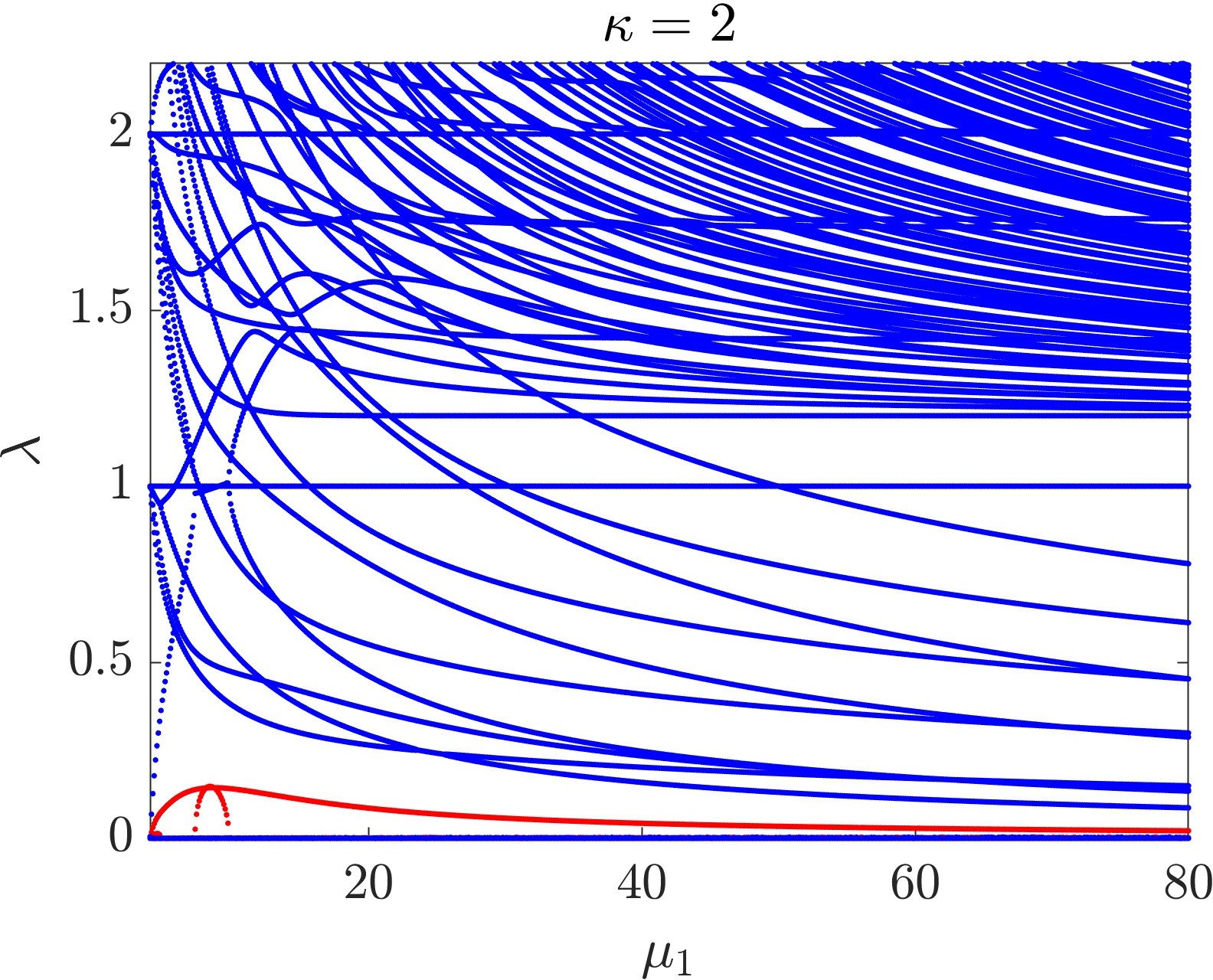
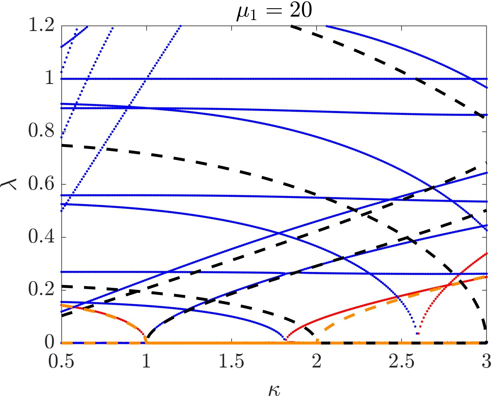
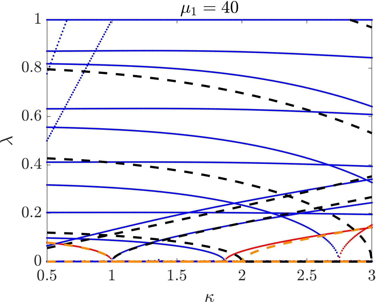
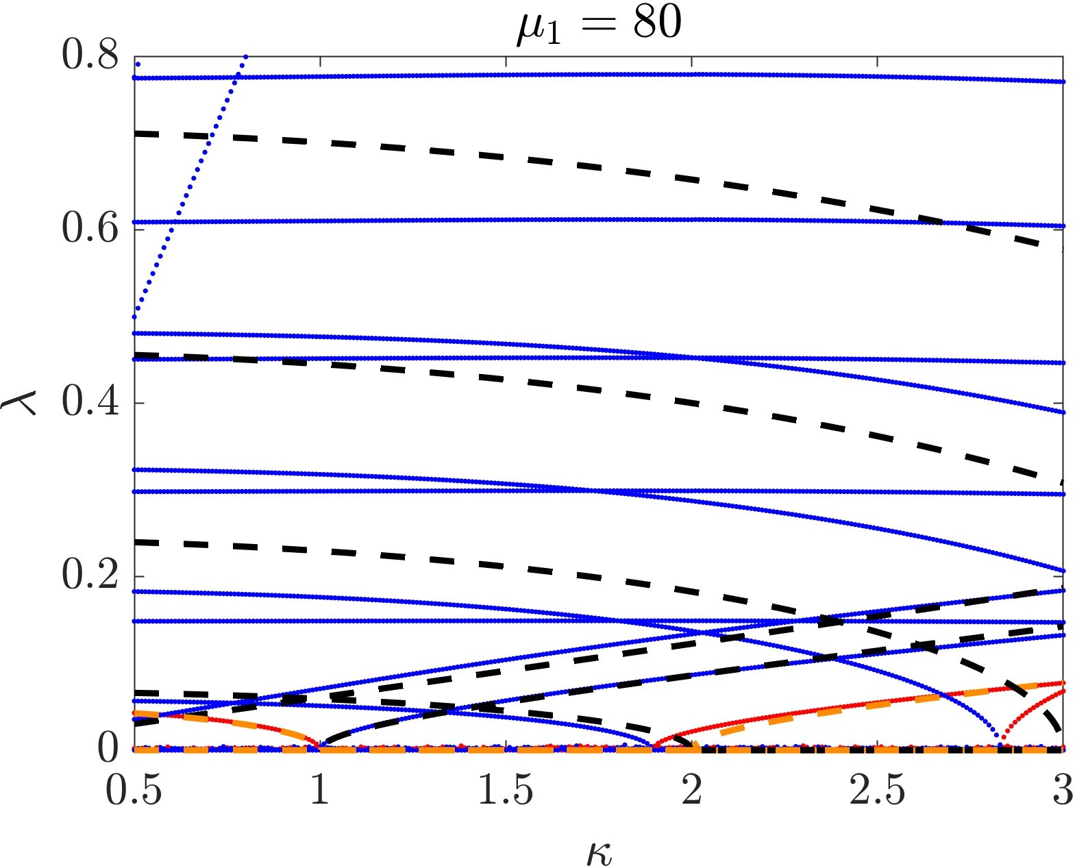
Figure 3: The BdG spectra of the VRB along the continuation path (of Eq. (43)) by varying the chemical potentials at fixed $\kappa=2$ (a) the real and imaginary parts of $\lambda$ are shown in red and blue, respectively. In (b-d), typical states in the TF regime are further continued in $\kappa$ from the above path at fixed chemical potentials $\mu_{1}=20,40$ and $80$, respectively. The gross feature is similar to that of the single-component VR, and the numerical spectra compare favourably with the analytically predicted spectra (of Eq. (42)) shown as dashed gold (real part) and dashed black (imaginary part) lines. Notice the improving nature of the analytical predictions as $\mu_{1}$ increases. See the text for more details and an analogous comparison with the VR spectra in Ticknor et al. (2018).

III Computational Setup

Our numerical computation includes identifying numerically exact VRB stationary states, characterizing their stability properties through the Bogolyubov-de Gennes (BdG) spectral analysis Pitaevskii and Stringari (2003); Kevrekidis et al. (2015), as well as exploring the VRB unstable dynamics. To find a stationary state, we apply the finite element method for a spatial discretization of the fields and subsequently utilize the Newton’s method for convergence given a suitable initial guess; see the parametric continuation below for the numerical continuation of the VRB states from its underlying analytic linear limit. Since the states are rotationally symmetric about the $z$-axis, we have identified them in the reduced $(\rho,z)$ cross section, where $\rho=\sqrt{x^{2}+y^{2}}$. Upon convergence, the BdG spectrum of the state is collected using the partial-wave method Wang et al. (2016); Wang and Kevrekidis (2017); Kollár and Pego (2011), again in the $(\rho,z)$ plane. In this work, we have collected the spectra of the pertinent low-lying angular Fourier modes $m=0,1,2,...,5$ Wang and Kevrekidis (2017). It is worth mentioning that this $2d$ reduced computation is far more efficient than a direct $3d$ computation, enabling us to investigate the VRB deep in the TF regime. Indeed, we have explored up to chemical potentials as large as $\mu_{1}=80$ for this three-dimensional structure in this work. Finally, when a genuinely $3d$ state is needed for dynamics, it is initialized from the $2d$ state using the cubic spline interpolation. Our dynamics is integrated using either the regular fourth-order Runge-Kutta method or a third-order operator splitting Fourier spectral method.

The VRB stationary states are parametrically continued from the underlying analytic linear limit at $(\mu_{1}=4,\mu_{2}=2)$ and $\kappa=2$. In this setting, the two small-amplitude fields decouple. The VR state is a complex mixing of the degenerate states of the ring dark soliton $(|200\rangle+|020\rangle)/\sqrt{2}$ and the planar dark soliton $|001\rangle$ with a relative phase of $\pi/2$. The bright component is in the $|000\rangle$ ground state. Here, $|mnp\rangle$ represents a $3d$ quantum harmonic oscillator state in the Cartesian coordinates. These linear states are used as the initial guess for slightly larger chemical potentials $(\mu_{1},\mu_{2})$ at fixed $\kappa=2$. When a solution is found near the linear limit, it is then used as the initial guess for larger chemical potentials at $\kappa=2$, and so on in this parametric continuation. By trial and error, we find that the following continuation path is both typical (the bright mass is neither too large nor small) and robust:

$$\mu_{2}=\mu_{1}-1.2-0.8\exp(-0.5(\mu_{1}-4)).$$ (43)

In addition, when the chemical potentials are sufficiently large (i.e., $\mu_{1}\gtrsim 10$), the existence of the VRB around this particular continuation path becomes robust and we can readily continue the states therein further in all other parameters, i.e., $\mu_{2}$, $\kappa$, and $g_{12}$. For example, for a typical $\mu_{1}$, $\mu_{2}$ can be tuned in a wide parametric range. The lower bound increases with increasing $\mu_{1}$ due to the tighter confinement of the vortex core and the upper bound is typically slightly below $\mu_{1}$. Here, the bright mass in the stationary state is tuned by adjusting $\mu_{2}$.

IV Numerical results

IV.1 Stationary states and the BdG spectra

Several typical numerically exact VRB configurations are depicted in Fig. 2. In this work, we have continued the VRB state following the continuation path of Eq. (43) from the linear limit all the way to $\mu_{1}=80$ which is deep in the TF regime at $\kappa=2$. Because the trap geometry is expected to have a strong influence on the VRB stability, we have explored the effect of $\kappa\in[0.5,3]$ at three typical chemical potentials at $\mu_{1}=20,40,80$.

The BdG spectra of the VRB along these four continuation paths are summarized in Fig. 3. Overall, the gross structure is qualitatively very similar to that of the single-component VR Ticknor et al. (2018). The $m=1$ mode becomes unstable exactly below $\kappa=1$, i.e., for prolate condensates. In the opposite direction, the $m=2$ mode becomes unstable at $\kappa>2$ (theoretically) and there is a finite chemical potential effect narrowing down the stability interval. The critical $\kappa$ moves closer to the theoretical limit $\kappa=2$ as $\mu_{1}$ is increased. Then, there is a similar trend for the $m=3$ mode, where the critical $\kappa$ moves towards the theoretical limit of $\kappa=3$ with an even stronger finite chemical potential effect. Between the two regimes, the VRB has a stable regime in the interval $1<\kappa\lesssim 2$. Therefore, the VRB is most stable in a slightly oblate condensate.

The numerical spectra also compare favourably with the corresponding theoretical prediction of Eq. (42), shown in dashed gold and dashed black lines for the real and imaginary parts, respectively. In Eq. (42), there is a fitting parameter $C_{\rm fit}$, which number is chosen to match the real part of the spectra, as motivated by the single-component VR work Ticknor et al. (2018). The $C_{\rm fit}$ is reasonably robust: our best fit at $\mu_{1}=20$ yields $C_{\rm fit}=2.5$, the ones at $\mu_{1}=40$ and $80$ are only slightly larger, yielding $C_{\rm fit}=2.6$ in both cases. The increasing stable mode with increasing $\kappa$ is the $m=0$ mode, the modes of $m=1,2,3$ can be readily identified due to their stability-instability transitions. Then, the yet higher-lying ones in increasing order correspond to $m=4$ and $5$, respectively. As $\mu_{1}$ increases, it is noted that the numerical spectra move closer to the theoretical predictions. This parallels the corresponding findings in the single-component VR comparison Ticknor et al. (2018), yet here we systematically generalize the results to the two-component VRB structure. Indeed, the latter is richer due to the modes associated with the presence of the second component. For example at $\mu_{1}=80$, the almost horizontal lines around Im$(\lambda)=0.15,0.3,0.45,0.6,0.75$ are due to $m=1,2,...,5$, respectively. Such almost horizontal and nearly equidistant lines in Figs. 3-3 correspond to the longitudinal modes. Mathematically, they are similar to sound modes in a 1D gas dynamics. In particular, the $m=1$ longitudinal mode, together with the $m=1$ transverse mode, produce the $m=1$ instability at larger $n_{2}$, as we see in Fig. 4.

IV.2 Effect of the bright mass

To understand the effect of the filled bright mass, it is helpful to compare the spectra of the VRB and VR in detail. To this end, we compare their stability intervals and typical growth rates qualitatively using several representative observables as summarized in Table 1. From these details, we identify the following features:

1. The critical $\kappa_{c}=1$ for the mode $m=1$ appears to be exact for both the VRB and VR. For higher Kelvin modes (i.e., modes of higher $m$), the critical $\kappa_{c}(m)\lesssim m$ and approaches $m$ as $\mu_{1}$ increases. In addition, large chemical potentials tend to decrease the unstable growth rates for both states.

2. The stability interval systematically shrinks when the VR is filled with a bright component, i.e., the bright component tends to narrow down the stability regime.

3. Interestingly, when both the VRB and VR are unstable, the bright component tends to decrease the corresponding growth rates. I.e., while the presence of the bright component expands the region of instability, it concurrently weakens the instability growth rates in the cases where the instability was already present. However, this is not strictly satisfied, e.g., the bright component enhances $\lambda_{r}(m=3,\kappa=3)$ at small chemical potentials, and then lowers it at larger ones.

Table 1: Some observables comparing the spectra of the VRB in Fig. 3 and the corresponding ones of VR Ticknor et al. (2018). Here, $\mu_{1}$ for the VR is understood as its chemical potential, and $\lambda_{r}=\mathrm{Re}(\lambda)$.

States	observables	$\mu_{1}=20$	$\mu_{1}=40$	$\mu_{1}=80$
VR	$\kappa_{c}(m=1)$	1	1	1
VR	$\kappa_{c}(m=2)$	1.86	1.9	1.92
VR	$\kappa_{c}(m=3)$	2.755	2.845	2.89
VR	$\lambda_{r}(m=1,\kappa=0.5)$	0.1572	0.09331	0.05435
VR	$\lambda_{r}(m=2,\kappa=2)$	0.08632	0.04619	0.02445
VR	$\lambda_{r}(m=3,\kappa=3)$	0.2931	0.1426	0.07254
VRB	$\kappa_{c}(m=1)$	1	1	1
VRB	$\kappa_{c}(m=2)$	1.815	1.87	1.895
VRB	$\kappa_{c}(m=3)$	2.595	2.75	2.83
VRB	$\lambda_{r}(m=1,\kappa=0.5)$	0.1434	0.07857	0.04306
VRB	$\lambda_{r}(m=2,\kappa=2)$	0.08574	0.04279	0.02149
VRB	$\lambda_{r}(m=3,\kappa=3)$	0.3391	0.1518	0.06821

The narrowing of the stability interval by the bright mass suggests a stability-instability transition when $\mu_{2}$ is tuned, at least for the $m\geq 2$ modes. This is indeed observed as we shall discuss below. However, it is interesting that we find the $m=0$ and $m=1$ modes can also have such transitions in this scenario. In addition, these instabilities are unprecedented in the VR context, to our knowledge, as the eigenvalues are complex ones. By contrast, the eigenvalue of the unstable $m=1$ mode below $\kappa=1$ is purely real. Our dynamic simulations confirm that the instabilities are indeed distinct ones, i.e., they appear to be genuinely caused by the interplay between the VR and the bright core and therefore they are not present in the single-component VR.

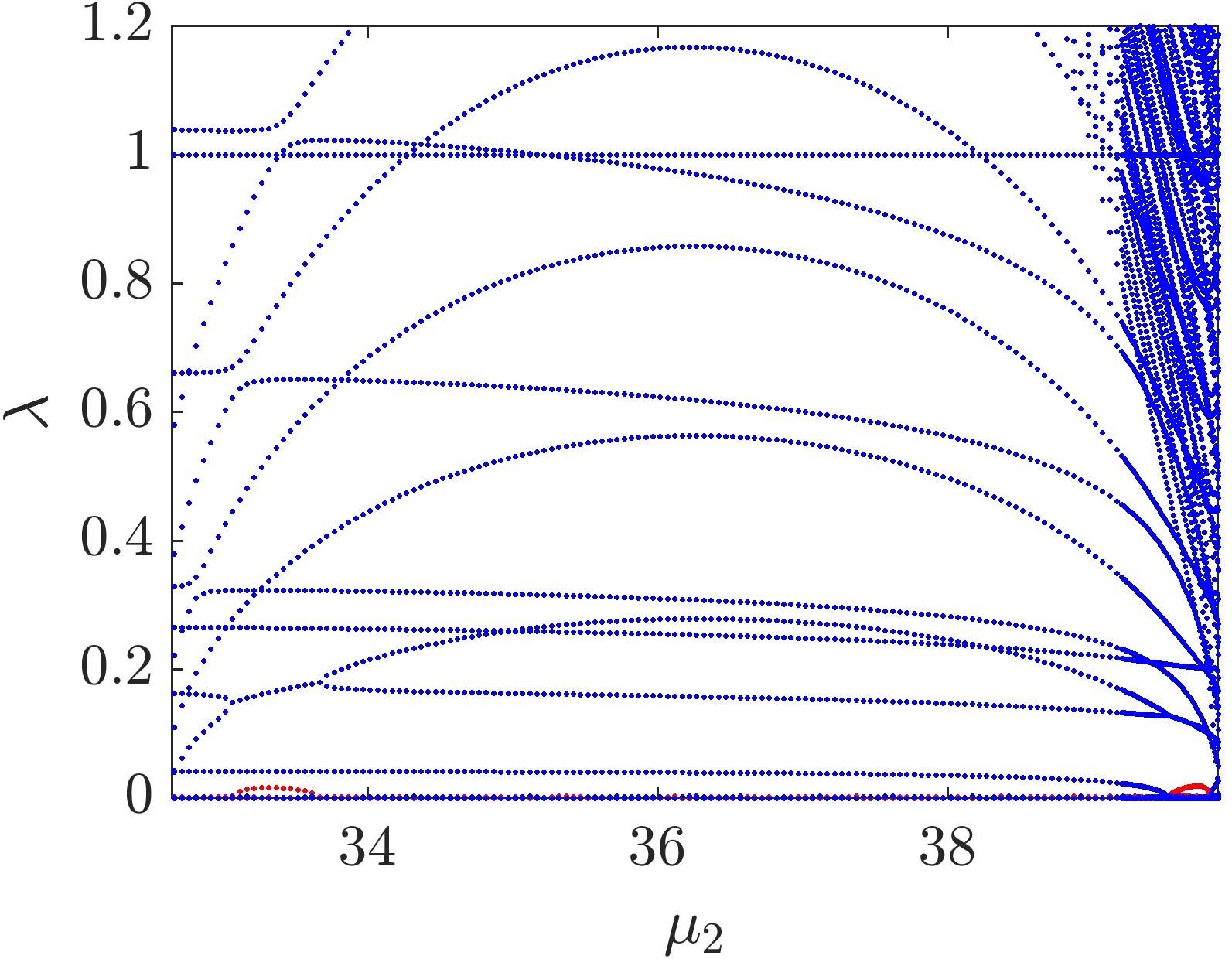
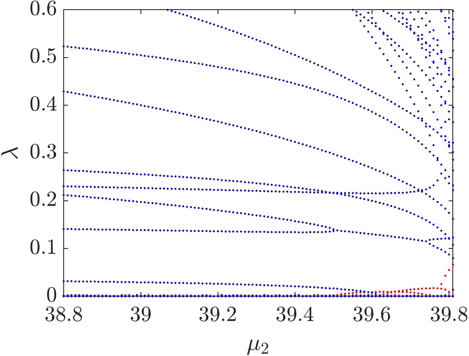
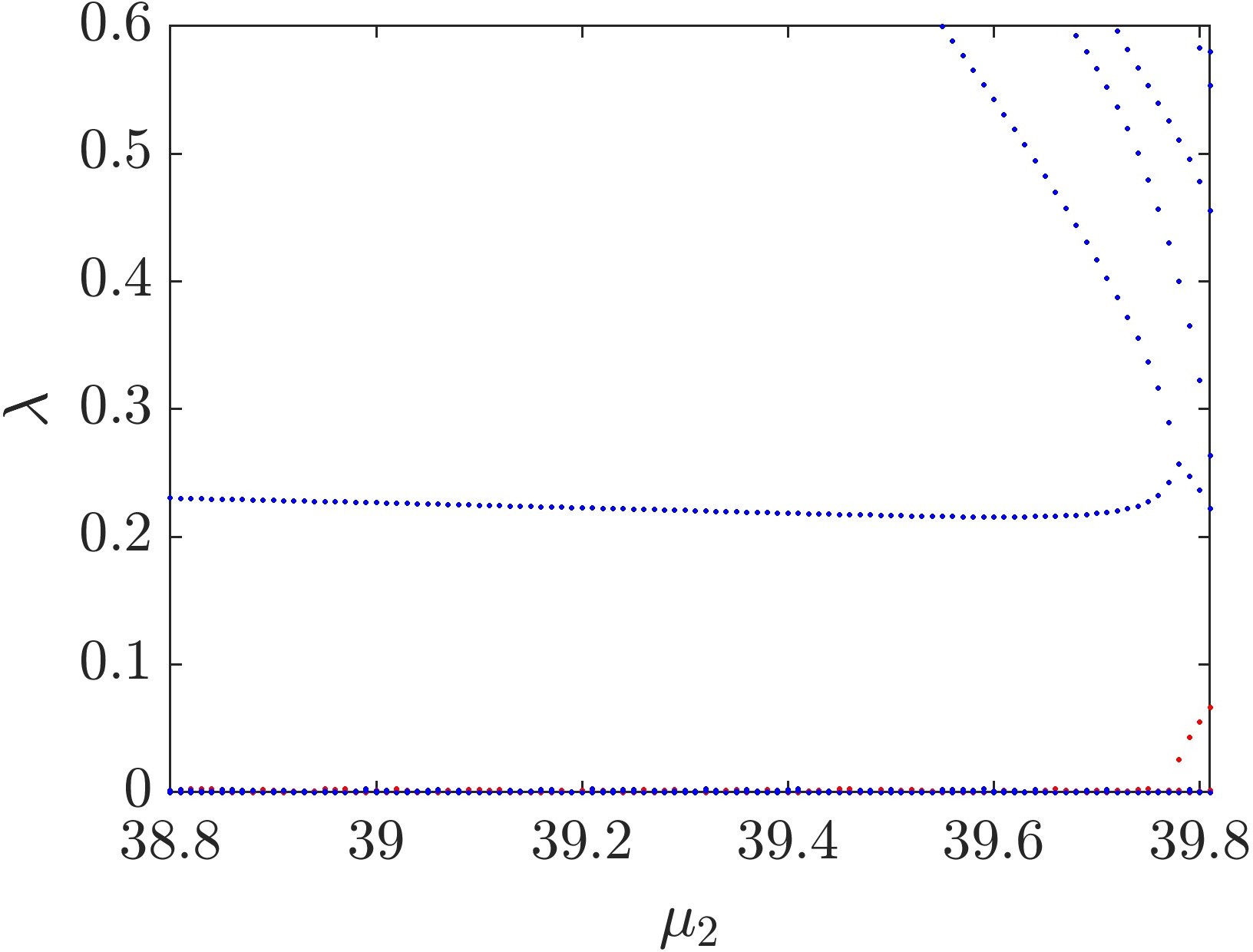
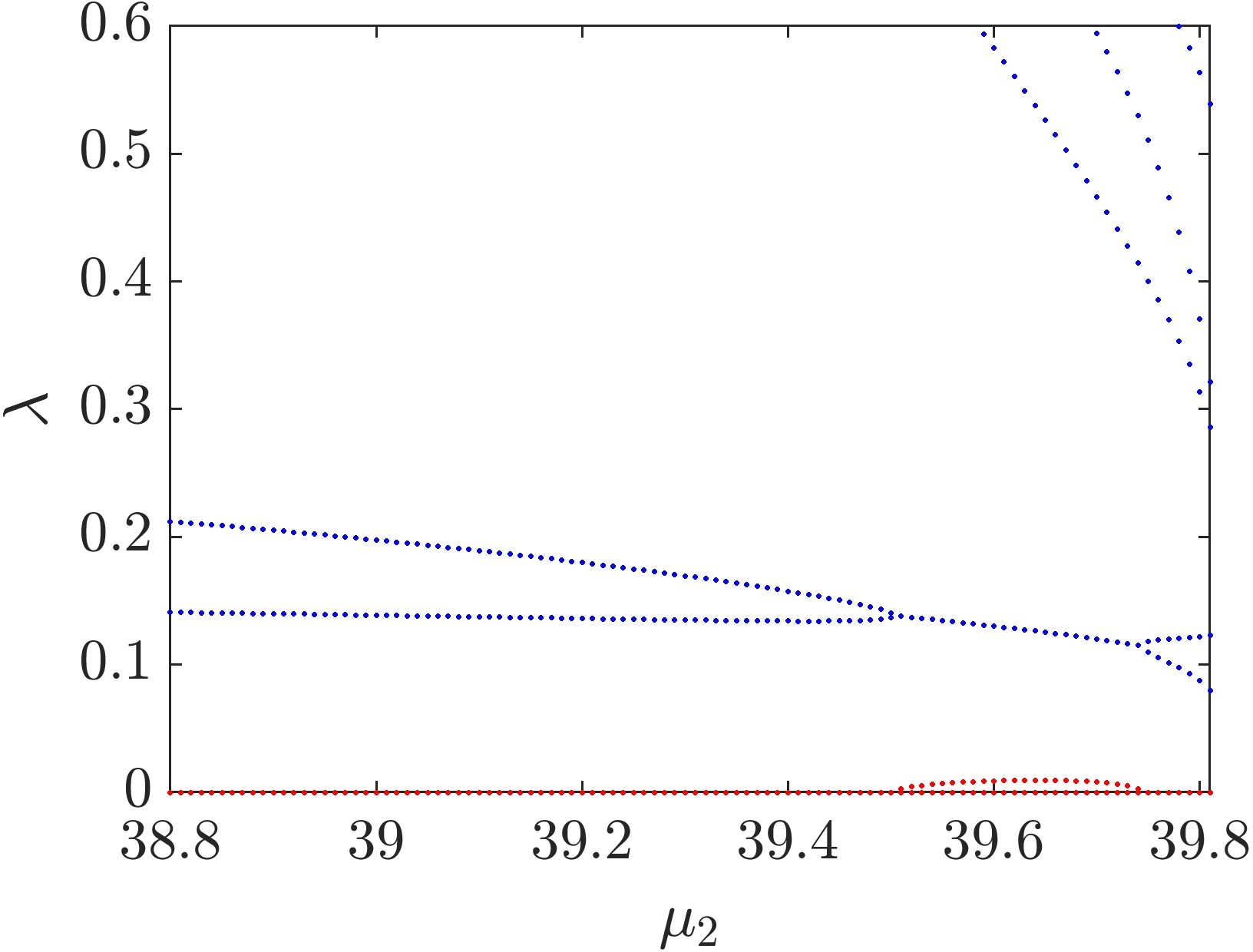
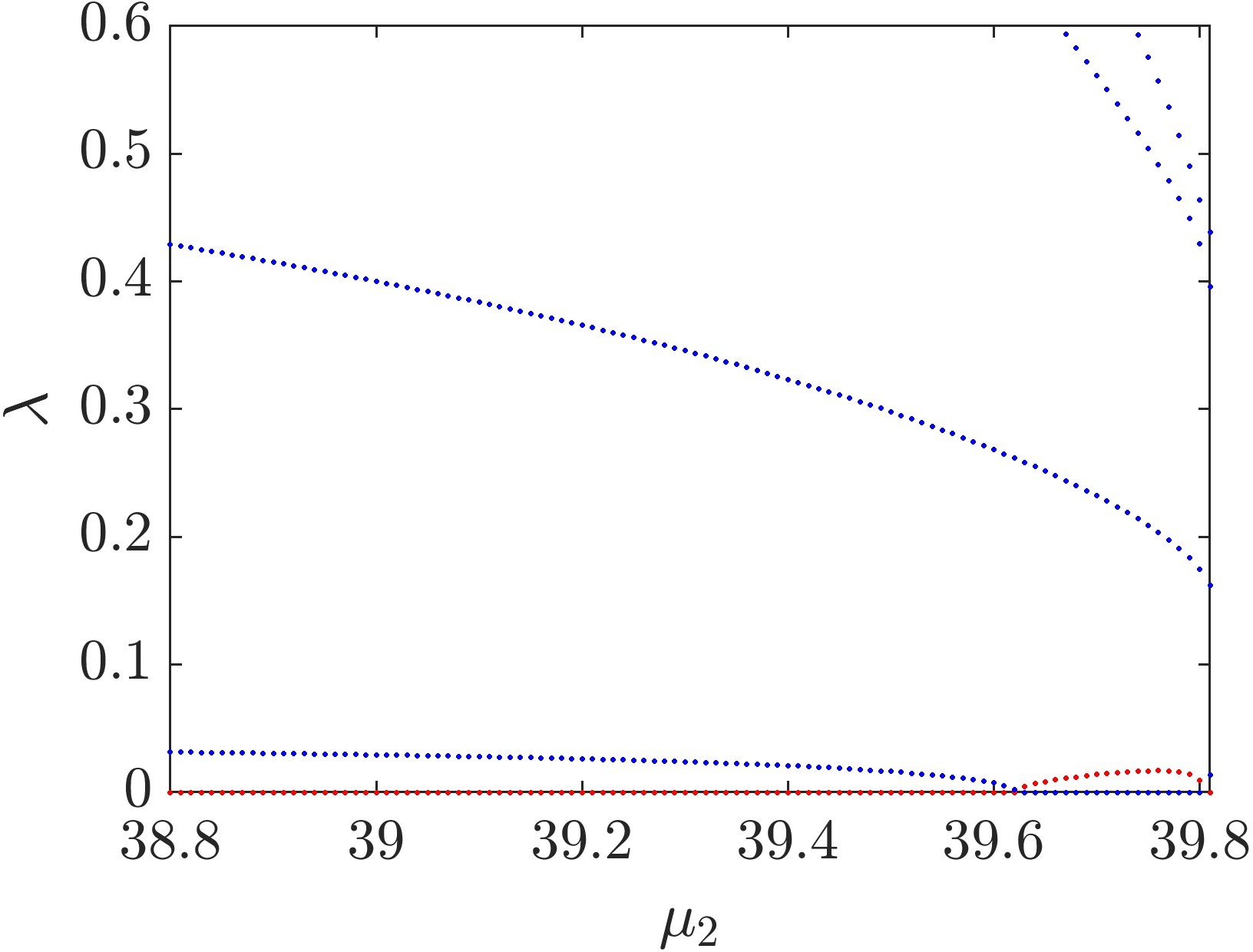
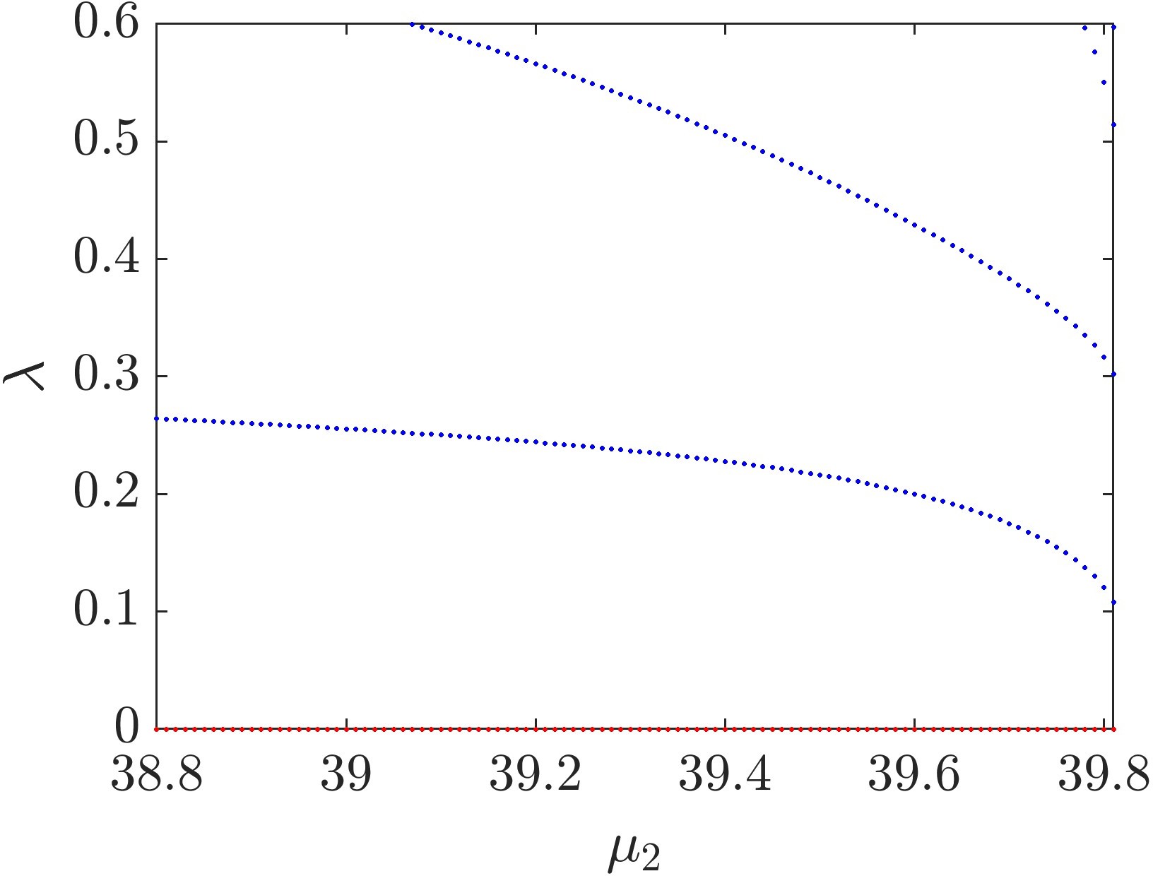
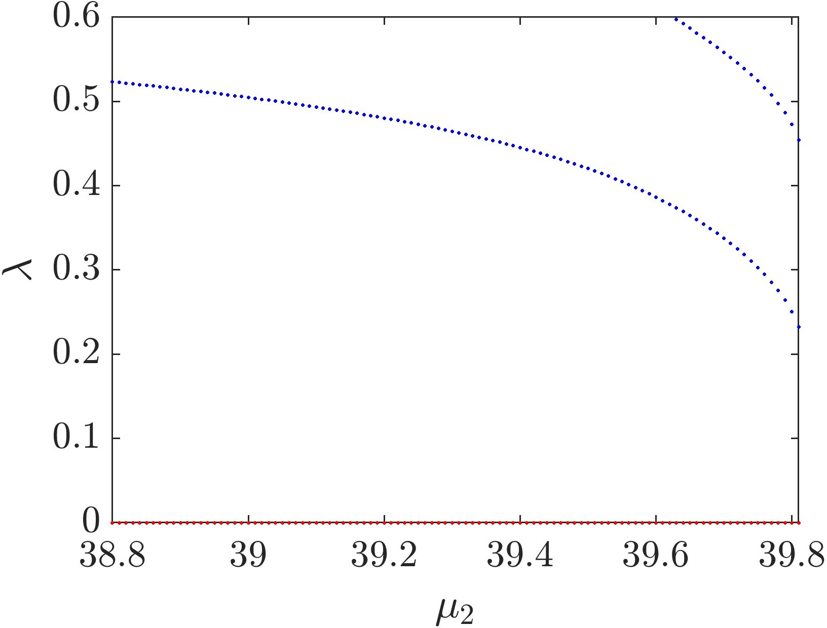
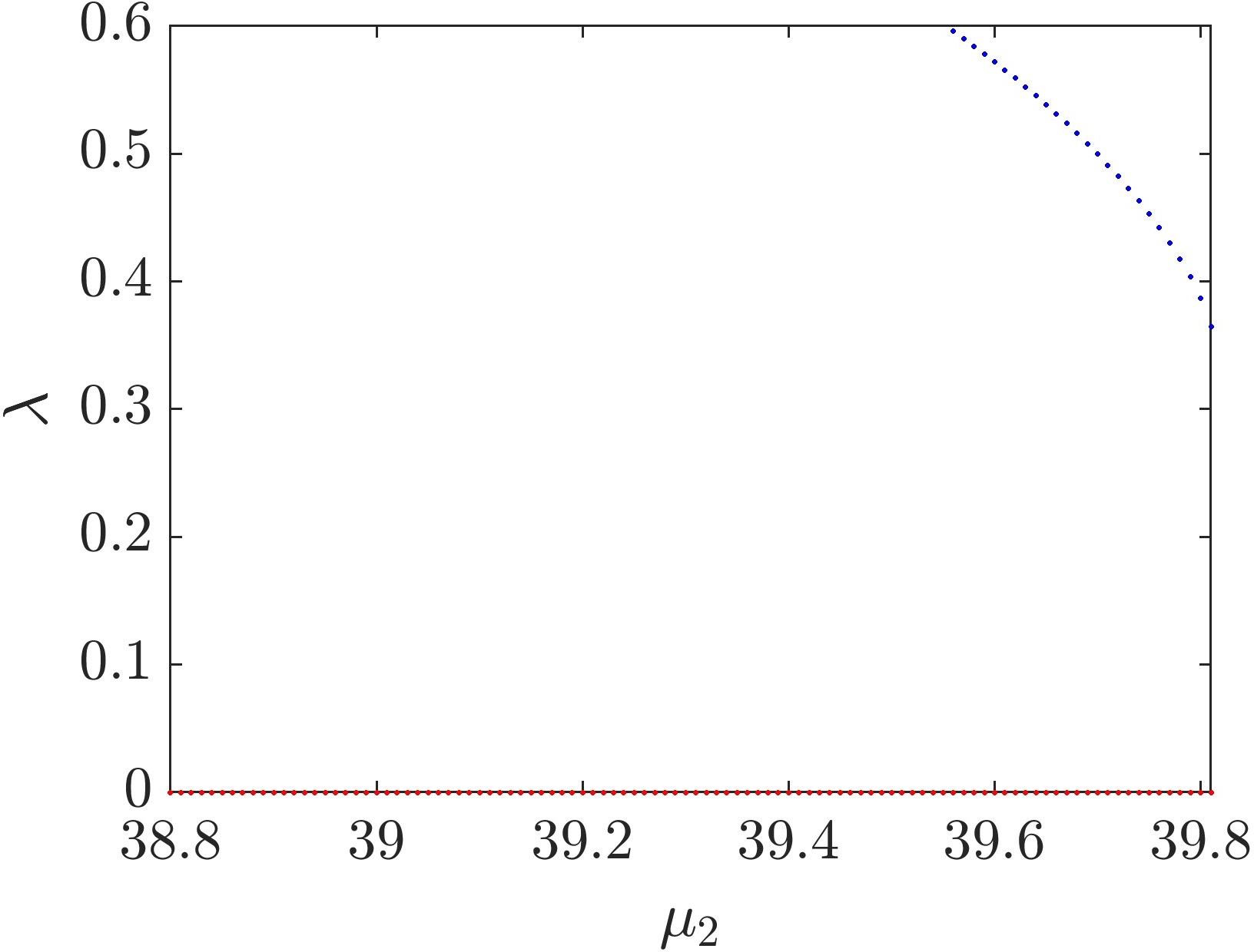
Figure 4: The first panel showcasing the BdG spectrum as a function of $\mu_{2}$ for a VRB illustrates the feature that $\mu_{2}$ can be tuned in a wide range in the TF regime, spanning from a vanishing number of atoms to a system-size bright component. When the bright mass is varied, the VRB may suffer intervals of instability. Here, $\mu_{1}=40$, $32.65<\mu_{2}<39.87$, $\kappa=1.8$, $g_{12}=1$. The second panel focuses on the relatively large $\mu_{2}$ regime for another typical case $\mu_{1}=40$, $\kappa=1.8$, but $g_{12}=1.01$. Detailed inspection shows that the $m=0,1,2$ modes can potentially become unstable as illustrated in the following panels depicting the spectra of the Fourier modes $m=0,1,...,5$, respectively. It should be noted that the $m=1$, $2$ instabilities are very common but the $m=0$ instability is only restricted to large fillings if it exists and frequently occurs in a rather narrow parametric regime.

Table 2: Some critical $\alpha$ and $\mu_{2}$ values when the bright mass is tuned at different $g_{12}$. Here, $\kappa=1.8$ and $\mu_{1}=40$.

$g_{12}$	$\alpha_{c}(m=1)$	$\alpha_{c}(m=2)$	$\mu_{2c}(m=1)$	$\mu_{2c}(m=2)$
1	0.1440	0.1440	39.52	39.52
1.01	0.0958	0.1345	39.5	39.62
1.02	0.0774	0.1238	39.53	39.71
1.03	0.0669	0.1158	39.58	39.8
1.04	0.0588	0.1061	39.63	39.88

We have conducted a systematic study of the VRB spectra by tuning $\mu_{2}$ at various values of $\kappa$ and $g_{12}$. The first panel of Fig. 4 illustrates a Manakov case, and $\mu_{2}$ is studied in its full range at $\mu_{1}=40$ and $\kappa=1.8$. This is achieved by starting from the state at $(\mu_{1},\mu_{2})=(40,38.8)$ and $\kappa=1.8$ in Fig. 3, and then tuning $\mu_{2}$ by either increasing or decreasing its value until the state no longer exists. As such, we find that the VRB exists for this particular case in a wide interval $32.65<\mu_{2}<39.87$, ranging from a faint bright soliton to a very fat core and also showing the robustness of the existence of the VRB structure at large $\mu_{1}$. The spectrum reveals an interesting feature that the bright component can introduce unstable intervals, and both the $m=1$ and $m=2$ modes can become unstable. To gain more intuition about the impact of the bright component mass, we introduce the mass ratio observable :

$$\alpha=N_{2}/N_{1}$$ (44)

complementing the more abstract $\mu_{2}$. Detailed inspection shows that the left instability (the one below $\mu_{2}=34$) is due to the mode $m=1$, but the mass ratio there is extremely small $\alpha\in[0.0004247,0.001128]$. On the other hand, both $m=1$ and $m=2$ modes become unstable when the filling is reasonably large $\alpha\gtrsim 0.1440$. The $m=1$ instability in the two intervals is oscillatory in nature, therefore differs from the $m=1$ instability in Fig. 3. By contrast, the $m=2$ instability is real and appears to be a regular one.

The instabilities in the relatively large $\alpha$ regime appear to be common for a wide range of $g_{12}$ and $\kappa$, and a typical spectrum at $g_{12}=1.01$ and $\kappa=1.8$ is also shown in Fig. 4. While the $m=1$ and $m=2$ modes become unstable simultaneously in the Manakov case, this appears to be an interesting coincidence and in general they do not bifurcate together at other $g_{12}$ and $\kappa$ values. Furthermore, an unstable $m=0$ mode is found despite the fact that it only occurs in the highly filled regime. However, it should be noted that the unstable interval thereof can be much narrower in other parametric regimes.

The critical $\alpha$ and $\mu_{2}$ of the modes with $m=1$ and $m=2$ for a few $g_{12}$ values are summarized in Table 2, and we shall explore the effect of $\kappa$ in the next subsection. As $g_{12}$ increases, the critical $\alpha$ decreases for both modes, and the $m=1$ mode bifurcates earlier than the $m=2$ mode at a smaller mass ratio. The decreasing of $\alpha$ here is reasonable, as the inter-component repulsion becomes stronger, it presumably does not take much bright mass to produce the same effective strength of interaction for the induced instabilities.

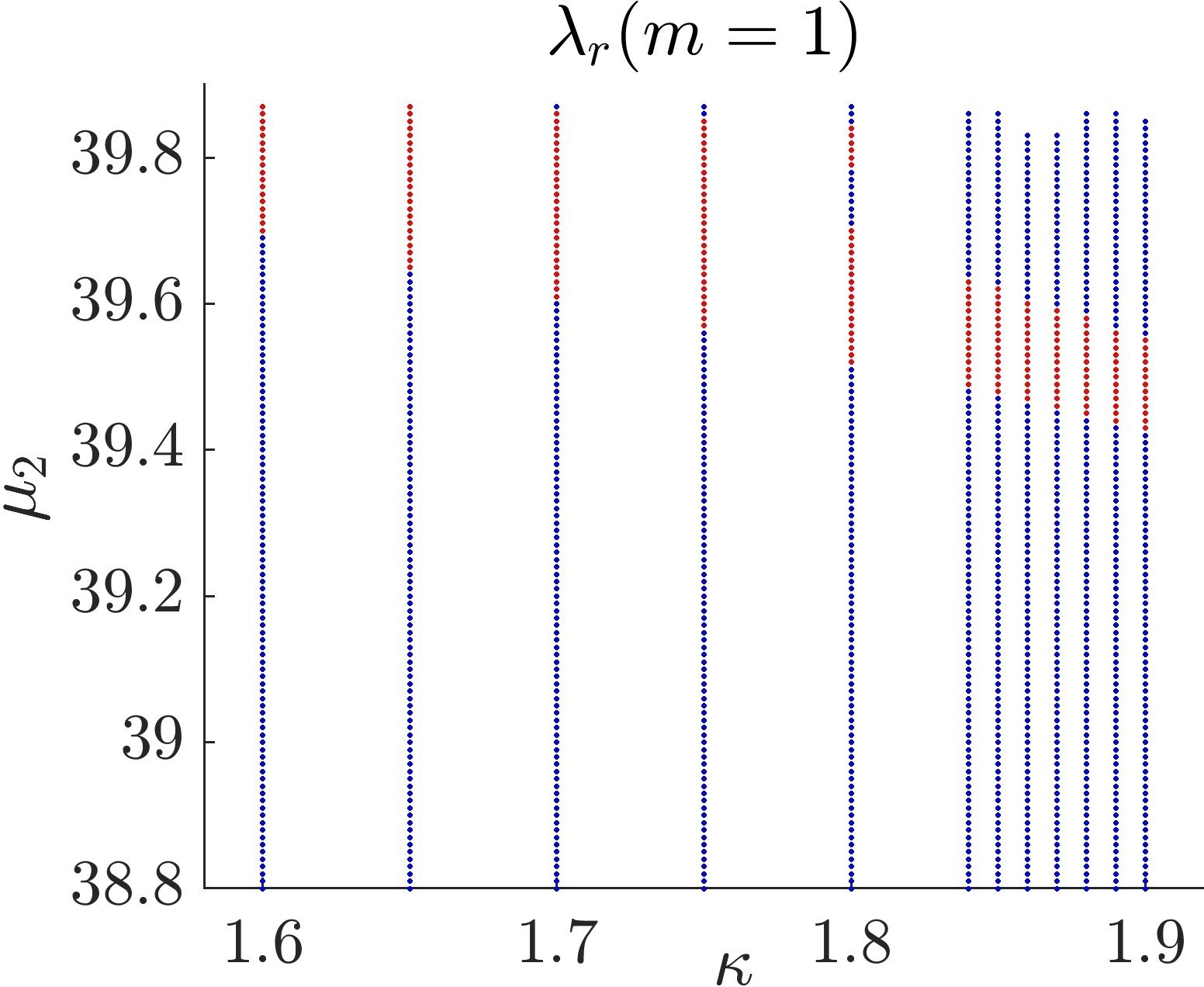
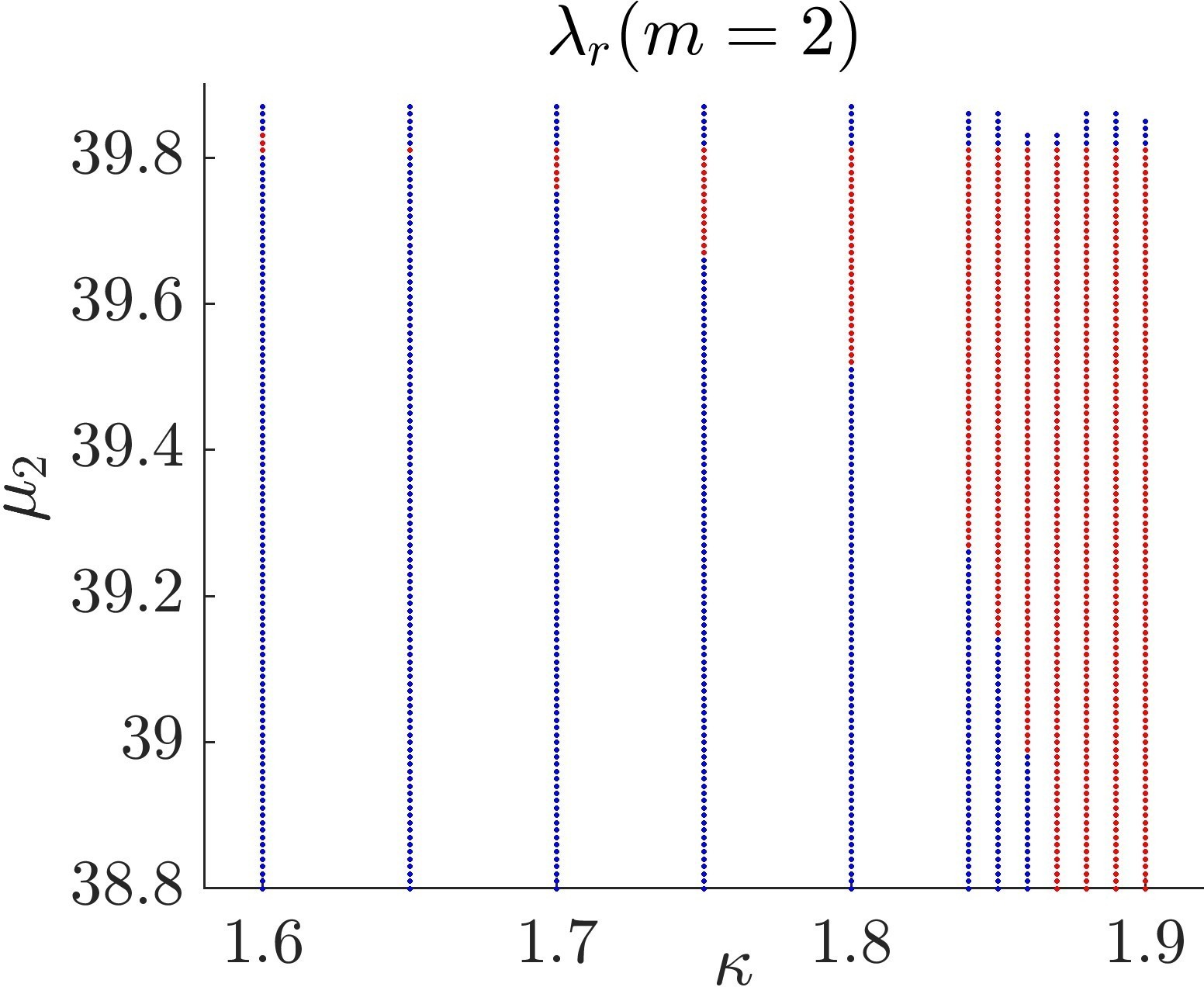
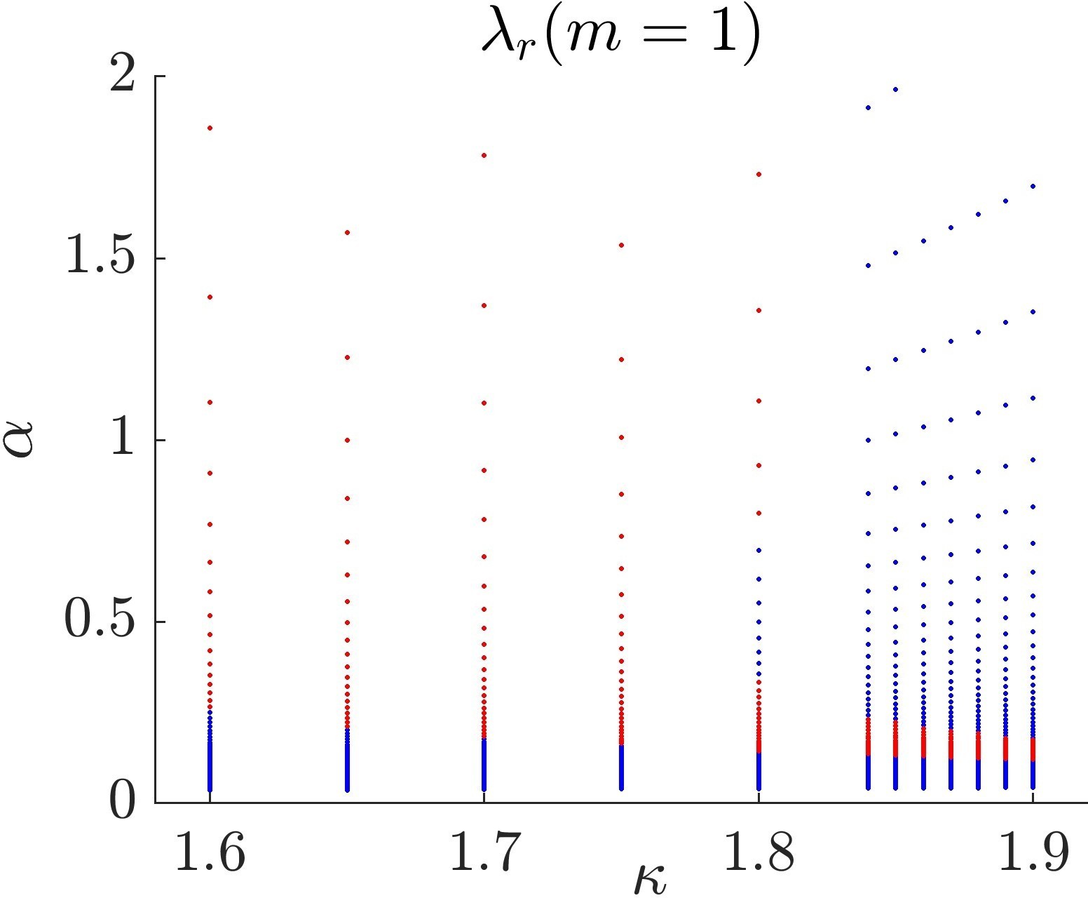
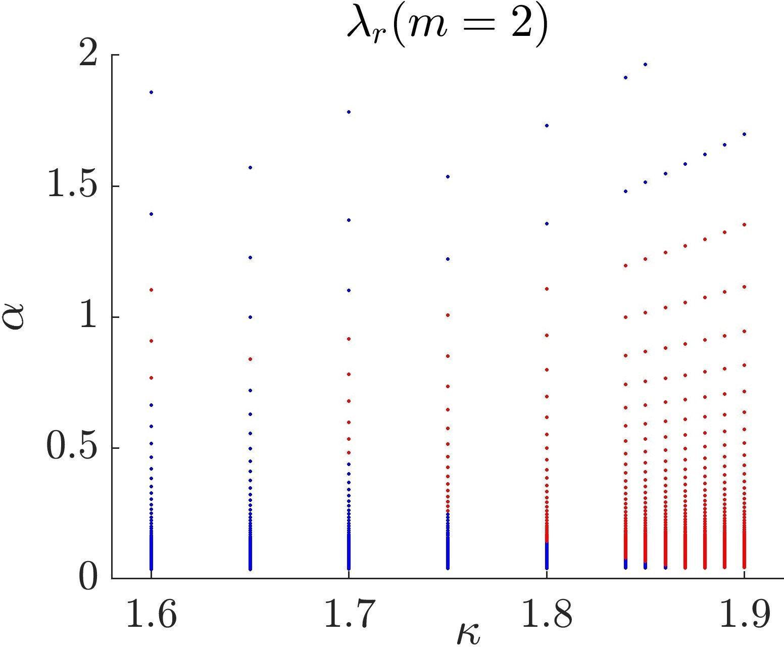
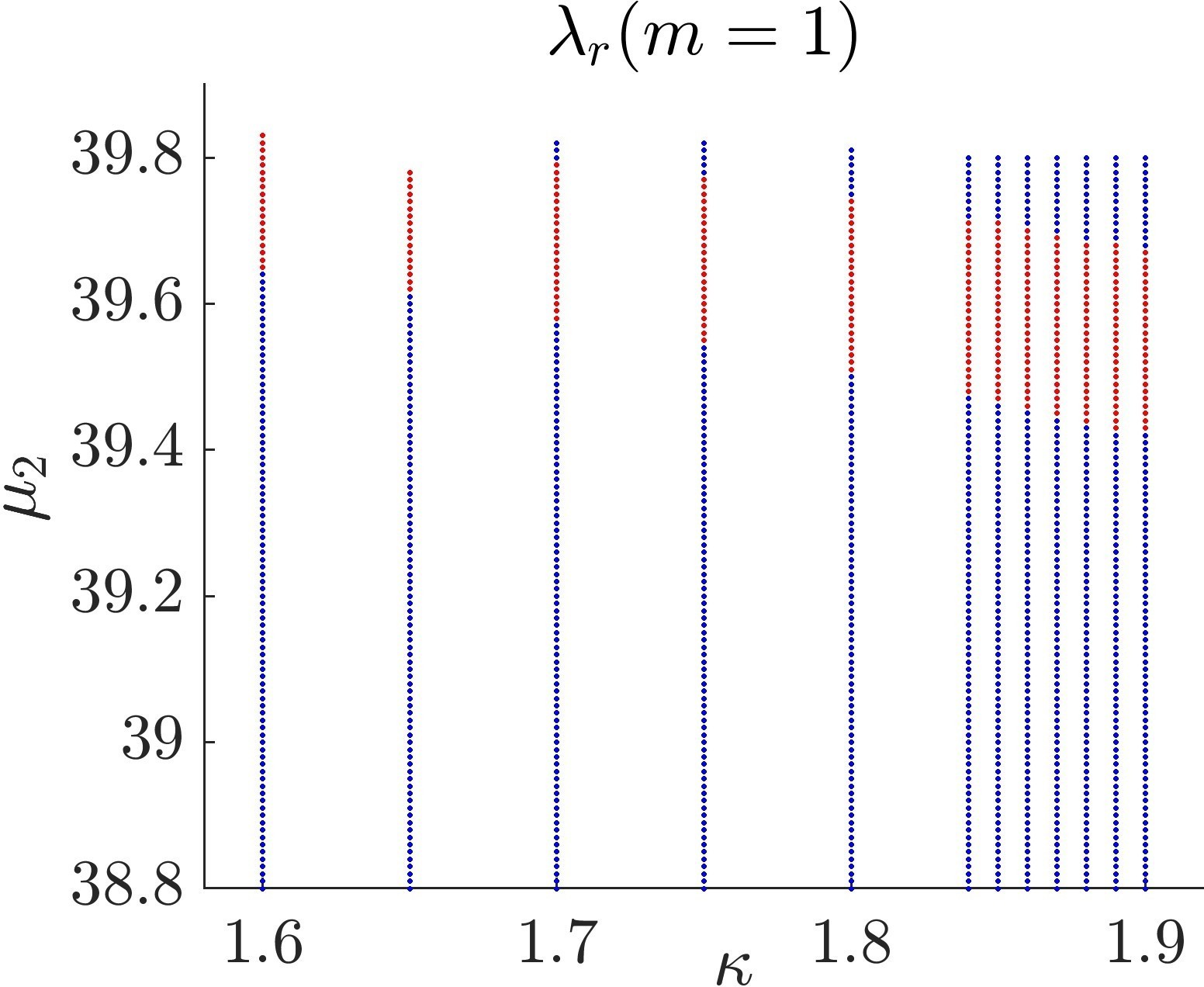
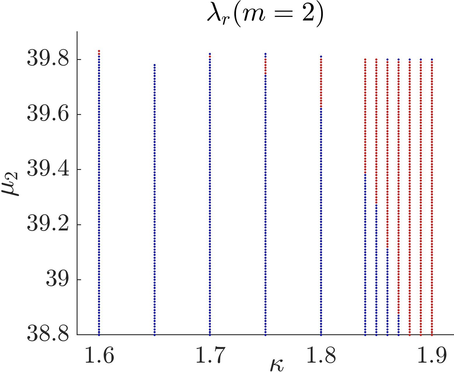
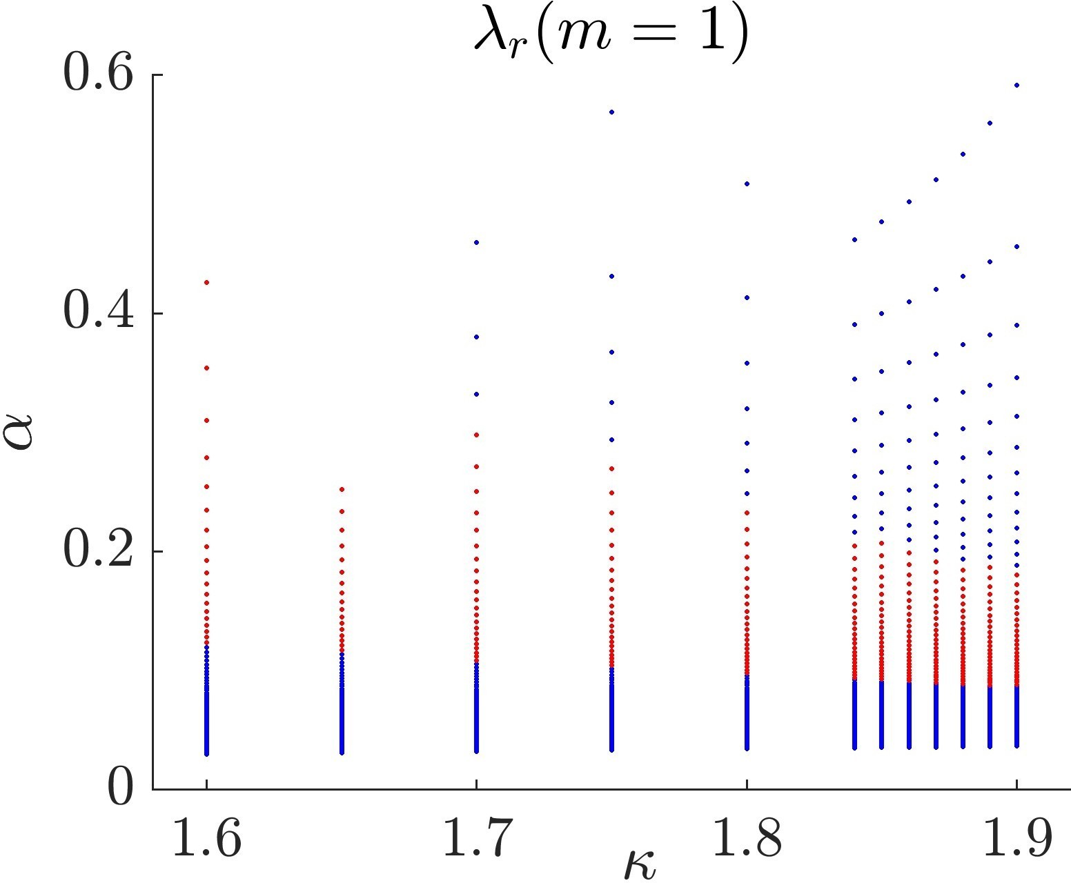
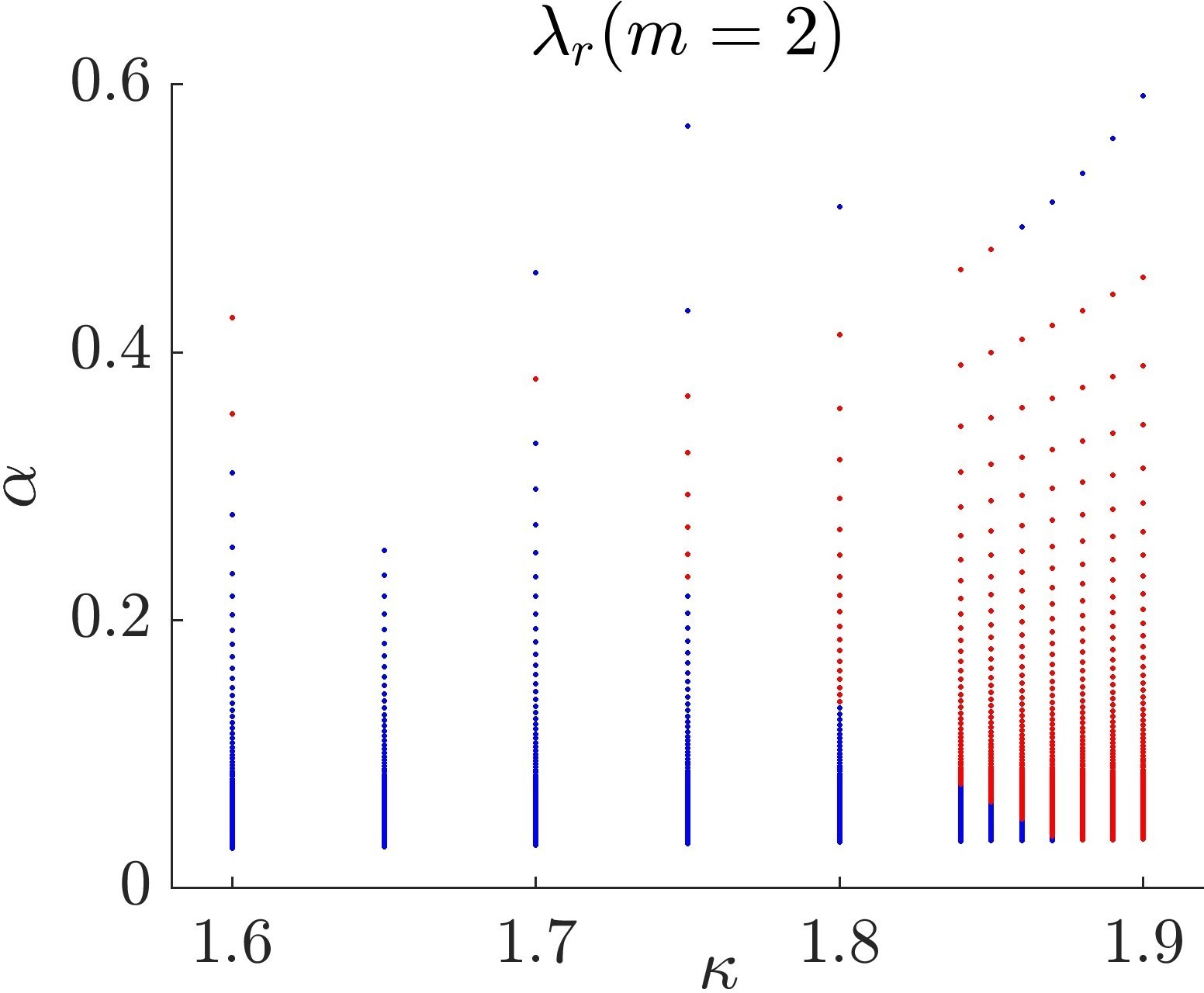
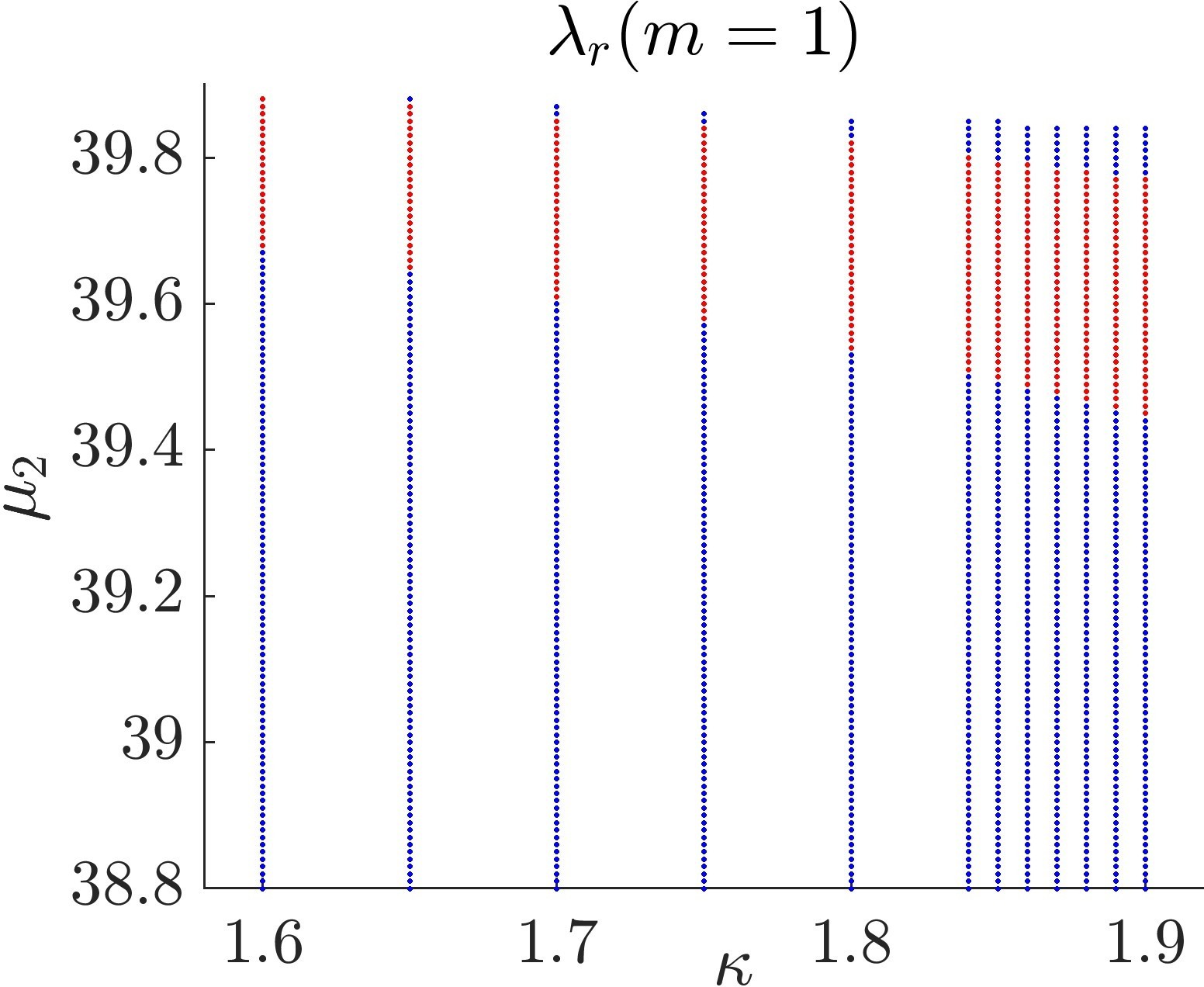
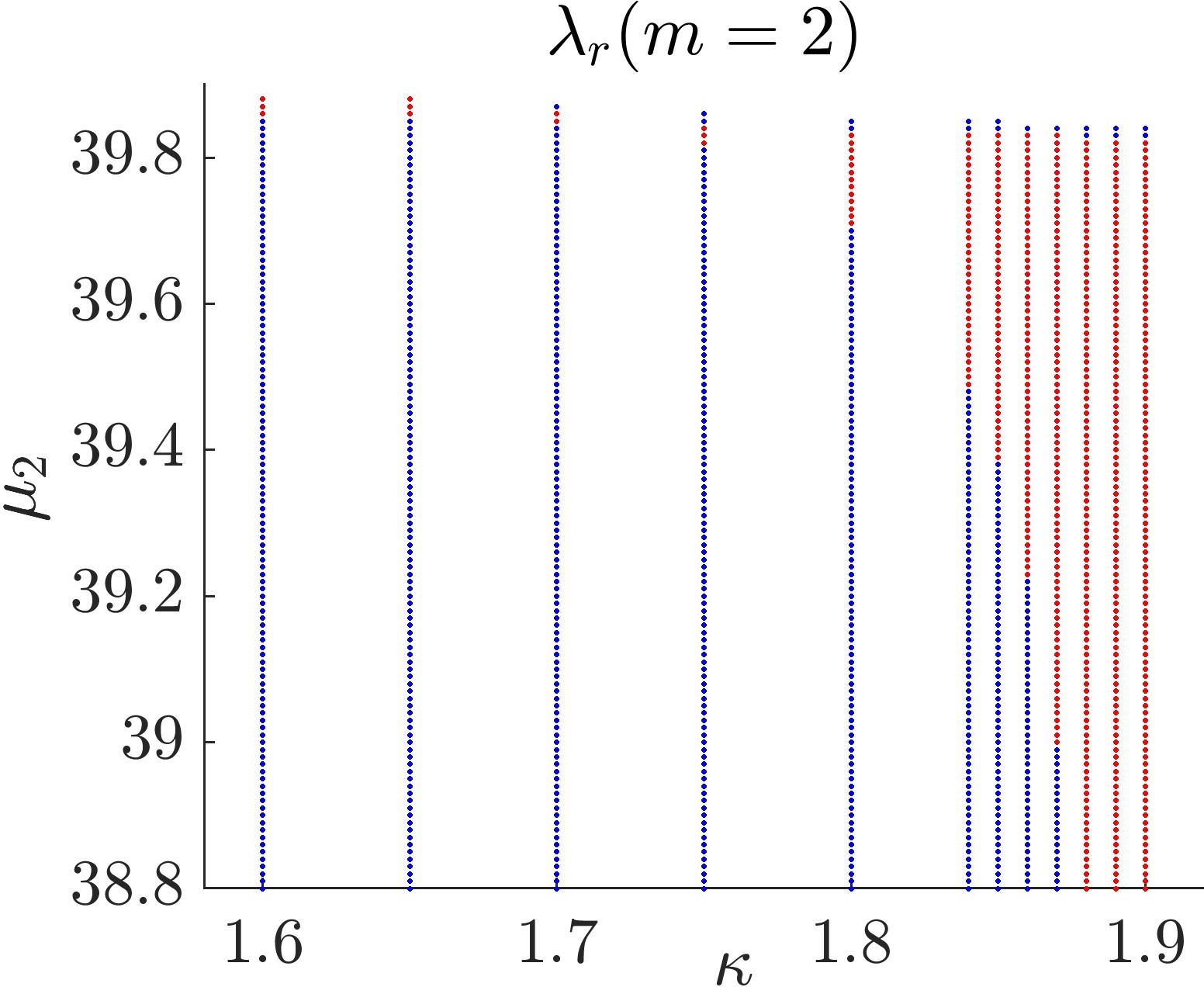
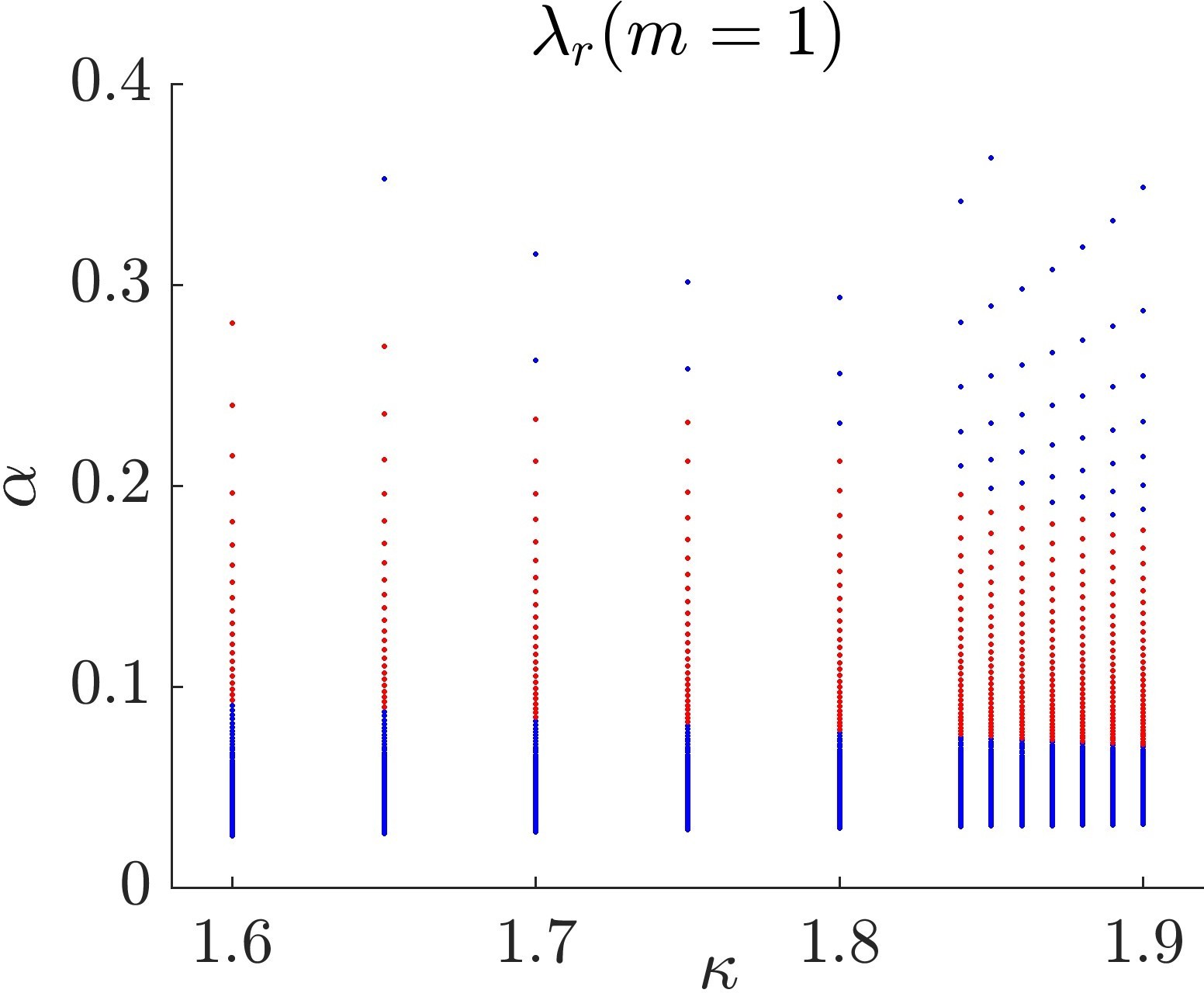
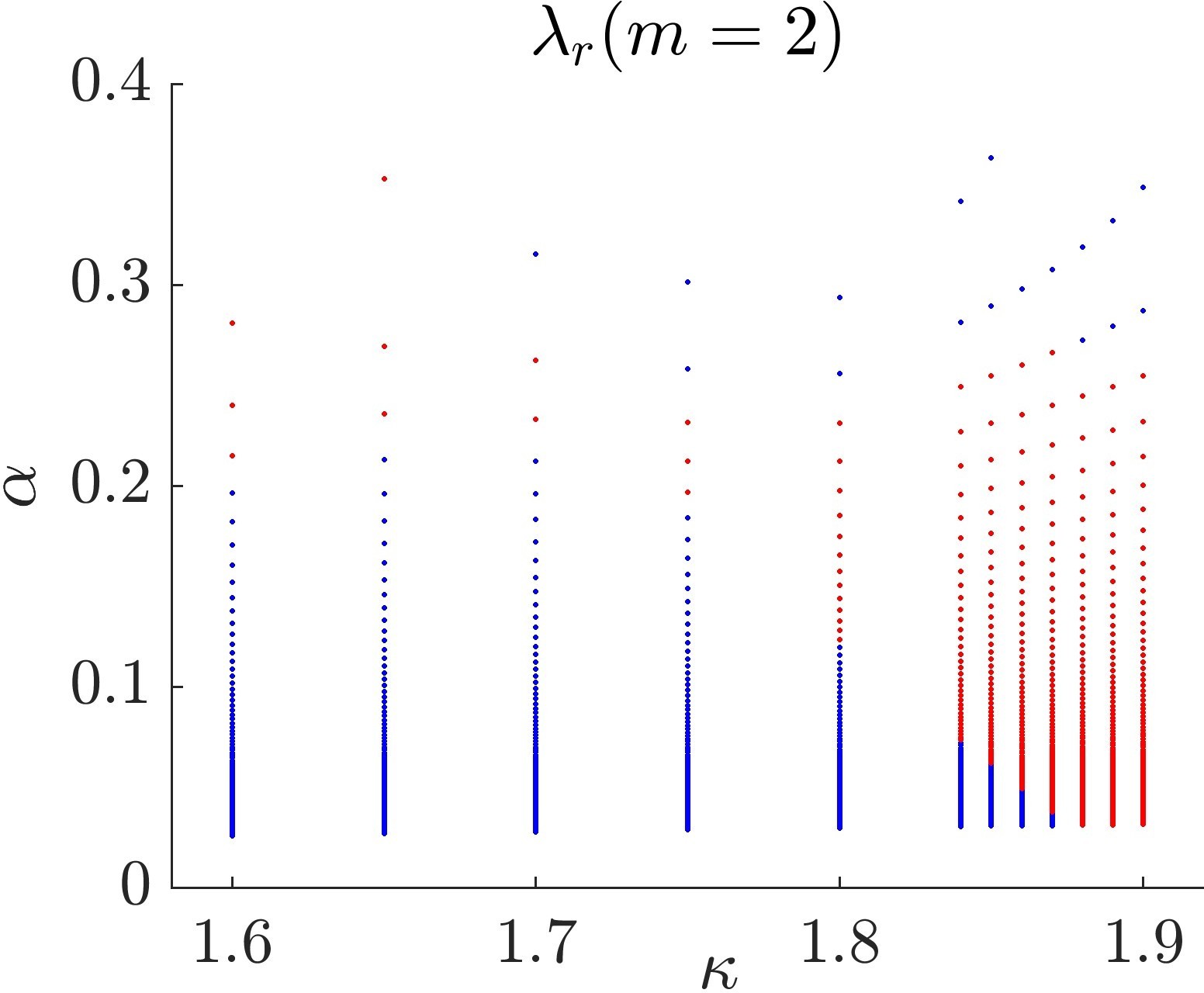
Figure 5: The effect of the bright mass on the VRB stability for various $\kappa$ and $g_{12}$ values. The rows in turn are for $g_{12}=1$, $1.01$, and $1.02$. Here, the blue points are for stable regimes and the red points are for unstable regimes. The maximum growth rate in an unstable interval is typically on the order of $O(0.01)$.

IV.3 Effect of $\kappa$ on the critical transitions

Here, we investigate the $\kappa$-dependence of the bright-induced instability in the large $\alpha$ regime. The examples shown in the previous subsection suggest that the critical transitions clearly depend on $\kappa$. To this end, we compute the spectra with respect to $\mu_{2}$ for a series of $\kappa$ values by further increasing $\mu_{2}$ to its upper limit from the appropriate states in Fig. 3. The results are illustrated in Fig. 5 and some typical numbers for the Manakov case are summarized in Table 3.

Since Fig. 3 shows that the $m=2$ instability is already present at $\kappa=1.87$ before $\mu_{2}$ is increased, this suggests that the critical chemical potential thereof should decrease when $\kappa$ is increased. This is found to be essentially the case numerically in Fig. 4 for both the $m=1$ and $m=2$ modes. However, the effect of $\kappa$ on the $m=2$ mode is stronger: note that the critical mass has a much larger slope for the $m=2$ mode. This produces an interesting exchange of bifurcation order as $\alpha$ increases at, e.g., $\kappa=1.8$ for the Manakov case. Above this value the $m=2$ instability bifurcates first, and below this value the $m=1$ instability bifurcates earlier instead.

Table 3: Some critical $\alpha$ and $\mu_{2}$ values with respect to $\kappa$ when the bright mass is tuned for the typical Manakov case in Fig. 5. The ones marked with a star (*) have rather narrow instability intervals. The “peculiar” trend of $\alpha_{c}(m=2)$ at $\kappa\lesssim 1.65$ is because in this regime, $\mu_{2c}$ essentially saturates, the drop of $\alpha$ at $\kappa=1.6$ is therefore dominated by the larger background size.

$\kappa$	$\alpha_{c}(m=1)$	$\alpha_{c}(m=2)$	$\mu_{2c}(m=1)$	$\mu_{2c}(m=2)$
1.60	0.2651	0.7675∗	39.70	39.81
1.65	0.2112	0.8379∗	39.65	39.81
1.70	0.1842	0.4370	39.61	39.75
1.75	0.1583	0.2606	39.56	39.67
1.80	0.1440	0.1440	39.52	39.52
1.84	0.1315	0.0789	39.48	39.26
1.85	0.1288	0.0658	39.47	39.15
1.86	0.1262	0.0525	39.46	38.99
1.87	0.1237	$<$0.042	39.45	$<$38.8
1.88	0.1213	$<$0.042	39.44	$<$38.8
1.89	0.1191	$<$0.043	39.43	$<$38.8
1.90	0.1169	$<$0.043	39.42	$<$38.8

It is noted that restabilization can occur when $\alpha$ is increased further, in line with the theoretical expectation, and more than one unstable intervals can also exist. Increasing $g_{12}$ has an effect of lowering the critical $\alpha$, but other than that, the general features remain largely similar to those of the Manakov case. It is worth mentioning that these instabilities are, however, quite weak and a typical maximum growth rate in an unstable interval is only approximately $O(0.01)$. In line with our theoretical expectation, no unstable modes for $m\geq 3$ are found in these wide parametric regimes.

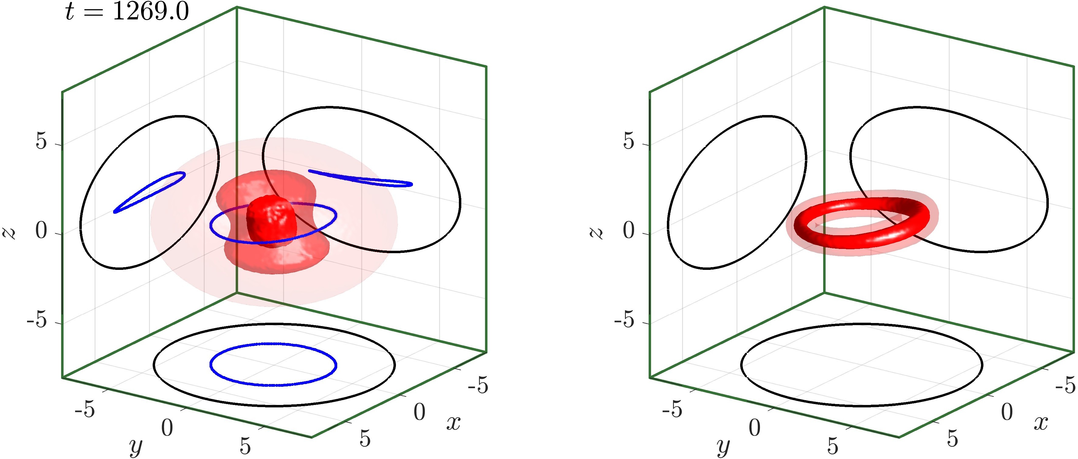
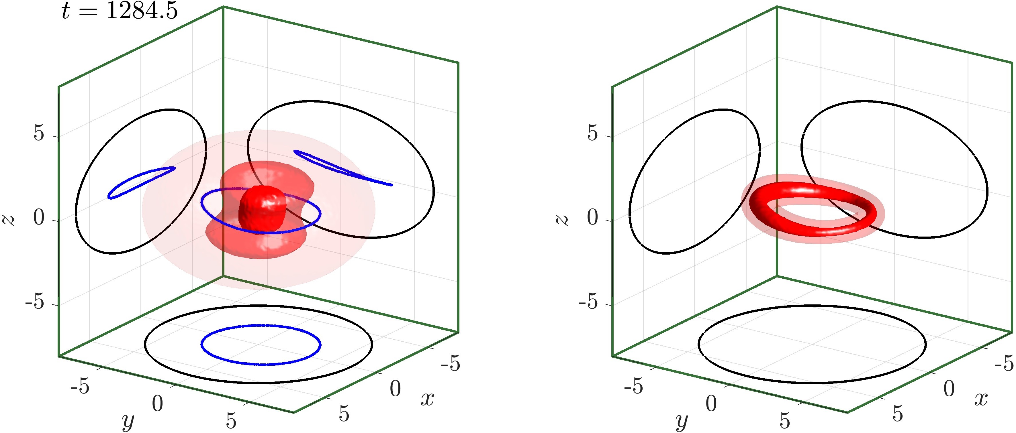
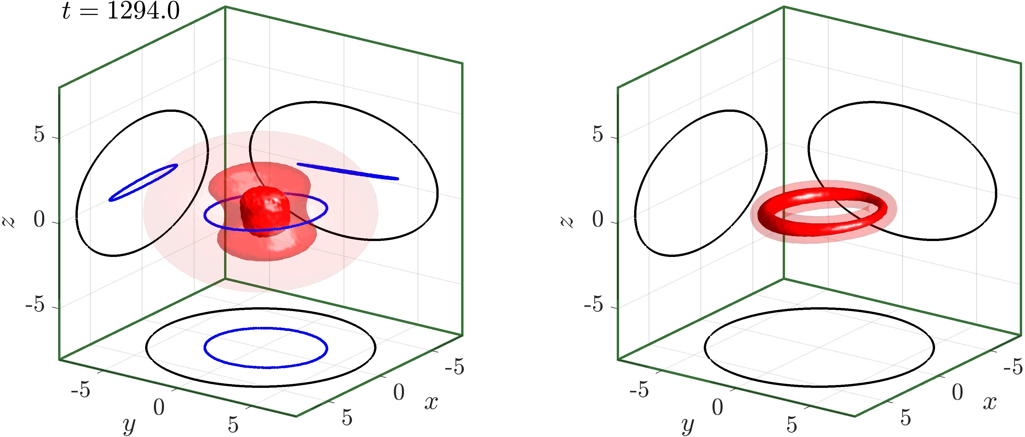
Figure 6: In the oscillatory $m=1$ unstable mode, the VRB first tilts and then propagates off the center, here in the approximately $-y$ direction at $t=1269$. The VRB then reaches the edge of the cloud and reverses its tilting direction. The VRB finishes the reversing at $t=1278.5$ and propagates in the opposite direction, passing through the center at approximately $t=1284.5$, and reaching the opposite end of the cloud. It similarly finishes reversing its tilting direction at $t=1294$ and then runs back to the trap center. The VRB reaches the trap center at $t=1300$, in a state similar to the one we started with at $t=1269$, and then continues the cycle. The oscillation amplitude, however, gradually increases and the VRB eventually breaks into VLB filaments; see the full movie for details VRB (a).

IV.4 Dynamical Simulations

We have conducted several typical dynamical simulations following the spectra. The unstable modes in Fig. 3 are similar to those of the single-component VR. For example, we have run three VRB dynamics with random perturbations at $\mu_{1}=20$ and $\kappa=0.9,2,3$, where the dominant unstable modes are $m=1,2,3$, respectively. First, it is worth mentioning that the bright mass essentially follows the VR core. At $\kappa=0.9$, the VRB tends to flip and meanwhile it also extends one of its ends towards the edge of the condensate. The VRB breaks into two pieces before almost making a full flip. At $\kappa=2$, the VRB breaks into two parallel vortex-line-bright (VLB) filaments extending outside the BEC. Then, the two VLBs can contract and reconnect into a full VRB. The VRB can repeat this process multiple times, with the two VLBs oriented towards different directions, before finally getting highly excited and disordered into vortical filaments. The instability at $\kappa=3$ is triggered much faster, and the VRB is broken into three VLBs following the $m=3$ mode as expected. Because these dynamics are similar to the VR counterparts, we shall not discuss them further here.

As mentioned earlier, we have also identified two unstable modes that are not available to the single-component VR, the oscillatorily unstable $m=1$ and $m=0$ modes. The former is very common but the latter is restricted to rather narrow chemical potential intervals of a large bright mass. We now discuss these two modes in detail.

The $m=1$ oscillatorily unstable mode is illustrated in Fig. 6. It might be appropriate to call it the VRB sloshing mode, as the VRB sloshes back and forth in the condensate. The VRB first tilts in the condensate and then propagates off the center, here in the approximately $-y$ direction at $t=1269$. The VRB then collides with the edge of the cloud and reverses its tilting direction. The VRB finishes the reversal at $t=1278.5$ and propagates in the opposite direction, passing through the center at approximately $t=1284.5$, colliding with the trap again on the other side and similarly finishes reversing its tilting direction at $t=1294$ and then runs back to the trap center. The VRB reaches the trap center at $t=1300$, in a state similar to the one we started with, and then continues this cycle. The oscillation amplitude, however, increases and the VRB eventually breaks into VLB filaments; see the full movie for details VRB (a). The simulation parameters are $\mu_{1}=20,\mu_{2}=19.4,\kappa=1.65,\alpha=0.2596,\lambda_{r}=0.006895$, and the $m=1$ mode is the only unstable mode.

The $m=0$ oscillatorily unstable mode is simpler to describe: this is the regular precessional mode of $m=0$ around its equilibrium state but with a growing amplitude. As the amplitude grows, Kelvin modes are naturally excited, leading to instabilities. Since the mode is relatively familiar, we shall not discuss it in further detail here, but a full movie thereof is available VRB (b). In this case, the $m=3$ mode is excited, and it is noticed that the VRB can break and reform for many cycles before the VRB is finally ejected out of the condensate. It is not very straightforward to find a parameter regime where $m=0$ is the only unstable mode, but it is possible to find a suitable regime where it dominates. For the state in the movie, $\mu_{1}=20,\mu_{2}=19.61,\kappa=1.7,\alpha=0.8306,\lambda_{r}(m=0)=0.02388,\lambda_{r}(m=1)=0.008185,\lambda_{r}(m=2)=0.006596$. Note that the bright mass is very large, with a remarkable filling fraction as large as $83$ percent.

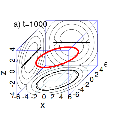
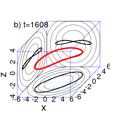
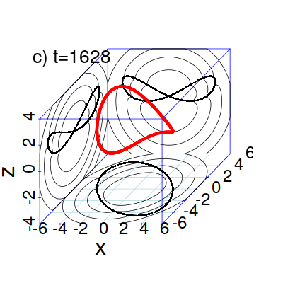
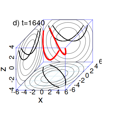
Figure 7: Snapshots of a vortex ring are shown for a parametric instability. The positions of the extracted vortex cores are shown as red points and their projections are shown on each plane along with the density contours of the BEC. In this example, we have picked $\mu=30$ with $\kappa=1.25$. A small displacement from a circular structure was initially induced with an $m=2$ mode in the radial direction.

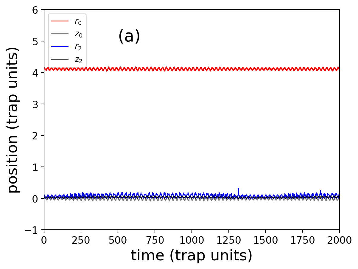
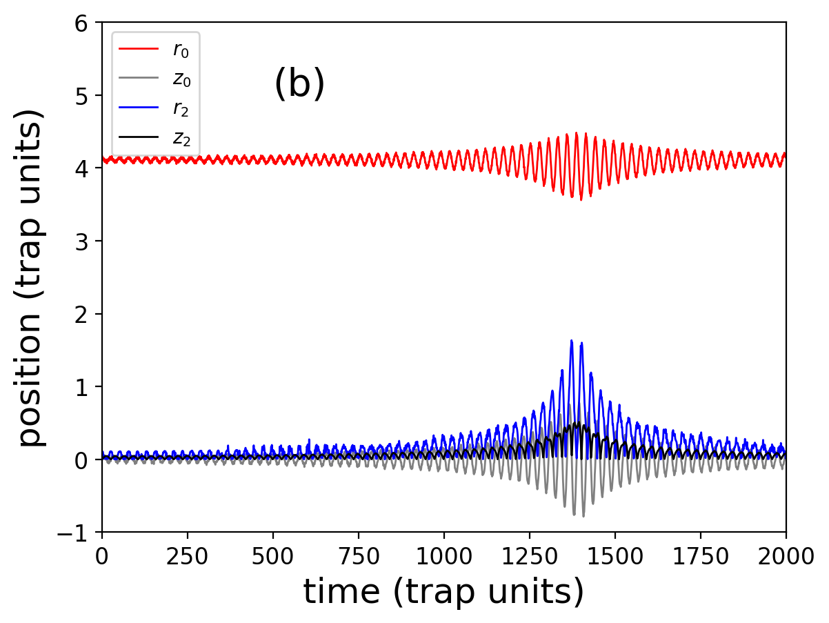
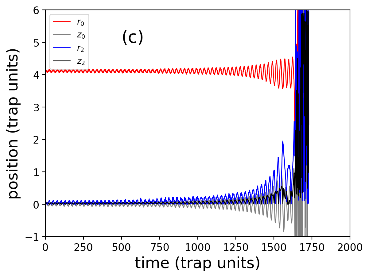
Figure 8: Several examples of the extracted modes associated with the vortex core positions (see Eq. (45)) are shown for different geometries: (a) $\kappa=1.27$, (b) $\kappa=1.255$, and (c) $\kappa=1.25$. The extracted vortex ring mode amplitudes shown are $r_{0}$ (red), $r_{2}$ (blue), $z_{0}$ (grey), and $z_{2}$ (black). In (a) a typical stable configuration with a seeded $m=2$ perturbation is shown. In (b) a configuration near the maximal response associated with the parametric instability has a growth and decay of a mode of the vortex ring. Another revival was observed (for longer times, not shown here) without the ring being broken. In (c) at the point of resonance, the ring breaks after being unstable at a time of around 1640 trap units. All simulations are for a single-component BEC with $\mu=30$.

IV.5 Nonlinear Parametric Instability

So far we have explored the linear instabilities of the VRB structure. Now, we turn to the nonlinear parametric instability analyzed qualitatively in Sec. II.4. Some numerical examples showcasing this instability are shown in Figs. 7 and 8. In Fig. 7 we show the vortex core locations by means of red points. Their projected positions are shown on each plane. In addition to the projected cores, we show the BEC density as thin contours at 0.2, 0.4, 0.6 and 0.8 of the maximum density. The BEC is started with the ring at 0.92 $R_{*}$ with a small amount of $m=2$ perturbation. After a long time, in this case about 1640 trap units of time, the $m=2$ mode grows and becomes unstable. The vortex ring stretches until the ring is broken by part of the ring leaving the BEC. This can be seen in Fig. 7(c) and (d). Notice that while the results here are shown for the case of a single-component VR, similar features arise in the case of the VRB.

Mode analysis, associated with this instability, is performed by extracting the core positions. These are sorted to be in azimuthal order. Then, analysis on the displacement and shape of the vortex ring was done assuming the following form for the vortex ring:

$$r(\varphi)=r_{0}+\sum_{m}r_{m}e^{im\varphi},\quad z(\varphi)=z_{0}+\sum_{m}z_{m}e^{im\varphi}.$$ (45)

Here $r$, $\varphi$, and $z$ are the cylindrical projections of $\bf R$. We have taken the real part of $z_{m}$ and the real and positive part of $r_{m}$. These have been plotted in Fig. 8. Here, the nonlinear parametric instability can be identified as occurring around $\kappa=1.25$. For$\kappa=1.27$, i.e., some distance parametrically away from this instability, the ring is stable. As $\kappa$ approaches the relevant parametric resonance point (from above) at $\kappa=1.255$, it is noted that the ring tends to become unstable but the instability can decay and thereby a stable ring is restored. Another revival was observed until the instability amplifies and eventually the ring breaks. At the resonance of $\kappa=1.25$, the ring becomes unstable quickly.

In other simulations, for example with $\kappa=1.14$, $n_{2}=78.5$, and $n_{1}=1570$, we observed similar behavior.

The parametric instability might be (partially) responsible for why the VR decays along some modes that are predicted to be linearly stable from the BdG spectrum Ticknor et al. (2018). It is therefore highly interesting to explore this type of resonance more systematically in the future, as it concerns a system that is linearly stable but nonlinearly unstable.

V Conclusions and Future Challenges

The properties of the VRB show significant similarities with the single VR, but also nontrivial differences. The bright component has an effect towards slowing down the unstable dynamics, i.e., decreasing the instability growth rate when the structure is (already at the single-component VR level) unstable. Nevertheless, at the same time, the presence of the second (bright, filling) component also typically narrows the stability regime in the parameter space, especially as concerns the higher wavenumber instabilities, such as $m=2$, $m=3$ and so on. Perhaps more importantly, the latter component can endow the structure with additional instabilities in a regime where the VR would be structurally stable. These instabilities may be weak, yet they are of interest given their diverse possible origin, both in terms of the mode responsible and the linear vs. nonlinear nature of the instability. For instance, we discussed herein (and qualitatively justified) the oscillatory instability arising from the $m=1$ mode, as well as the rather narrow instability of the $m=0$ mode at the linear (spectral) level. There are also nonlinear, parametric instabilities that are present, arising from the resonance of modes such as $m=0$ and $m=2$, as we have also elucidated.

Naturally, there are numerous future directions that are emerging as a result of the present work. One important aspect of consideration of such topologically charged states is the consideration of not only density-induced (spin-independent) effects as is the case herein, but also of spin-dependent ones that arise in $F=1$ and $F=2$ spinor condensates Kawaguchi and Ueda (2012); Stamper-Kurn and Ueda (2013). Hence, extensions of considerations to similar (but also Skyrmion) structures in 3-component BECs and beyond constitute a natural extension of the present work. Additionally, the recent exploration of advanced numerical methods, such as deflation Boullé et al. (2020) has enabled the characterization of far more elaborate topological structures in single-component, three-dimensional condensates. It would be of particular interest to examine generalizations of such states in multi-component settings and to examine their associated mechanisms of instability. Lastly, and similarly to the extensions of a single VR to multiple ones in single-component BECs Wang et al. (2017), the interaction of a VRB with a VR or with another VRB would be interesting to quantify from an analytical and numerical perspective. Such studies will be reported in future publications.