Quintic-scaling rank-reduced coupled cluster theory with single and double excitations

Abstract

We consider the rank-reduced coupled-cluster theory with single and double excitations (RR-CCSD) introduced recently [Parrish et al., J. Chem. Phys. 150, 164118 (2019)]. The main feature of this method is the decomposed form of the doubly-excited amplitudes which are expanded in the basis of largest magnitude eigenvectors of the MP2 or MP3 amplitudes. This approach enables a substantial compression of the amplitudes with only minor loss of accuracy. However, the formal scaling of the computational costs with the system size ($N$) is unaffected in comparison with the conventional CCSD theory ($\propto N^{6}$) due to presence of some terms quadratic in the amplitudes which do not naturally factorize to a simpler form even within the rank-reduced framework. We show how to solve this problem, exploiting the fact that their effective rank increases only linearly with the system size. We provide a systematic way to approximate the problematic terms using the singular value decomposition and reduce the scaling of the RR-CCSD iterations down to the level of $N^{5}$. This is combined with an iterative method of finding dominant eigenpairs of the MP2 or MP3 amplitudes which eliminates the necessity to perform the complete diagonalization and making the cost of this step proportional to the fifth power of the system size, as well. Next, we consider the evaluation of the perturbative corrections to the CCSD energies resulting from triply excited configurations. The triply-excited amplitudes present in the CCSD(T) method are decomposed to the Tucker-3 format using the higher-order orthogonal iteration (HOOI) procedure. This enables to compute the energy correction due to triple excitations non-iteratively with $N^{6}$ cost. The accuracy of the resulting rank-reduced CCSD(T) method is studied both for total and relative correlation energies of a diverse set of molecules. Accuracy levels better than 99.9% can be achieved with a substantial reduction of the computational costs. Concerning the computational timings, break-even point between the rank-reduced and conventional CCSD implementations occurs for systems with about $30-40$ active electrons.

I Introduction

With the coupled-cluster (CC) theory Crawford and Schaefer III (2007); Bartlett and Musiał (2007) firmly established as a powerful electronic structure method, applying it to large molecules remains a considerable challenge. Such applications are limited by unfavorable scaling of the computational costs with the size of the system. For example, the “gold standard” electronic structure method – CC model with single and double excitations (CCSD) augmented with perturbative triples correction [CCSD(T)] – scales as the seventh power of the system size Raghavachari et al. (1989). This makes canonical CCSD(T) calculations for molecules larger than $20-30$ atoms extremely expensive, assuming that a basis set of at least triple-zeta quality is used. To an extent, this boundary can be pushed by massive parallelization of the code Kobayashi and Rendell (1997); Hirata (2003); Auer et al. (2006); Olson et al. (2007); Janowski, Ford, and Pulay (2007); Janowski and Pulay (2008); van Dam et al. (2011); Deumens et al. (2011); Anisimov et al. (2014); Solomonik et al. (2014); Calvin, Lewis, and Valeev (2015); Peng et al. (2016); Lyakh (2019); Gyevi-Nagy, Kállay, and Nagy (2020); Peng et al. (2020); Datta and Gordon (2021); Gyevi-Nagy, Kállay, and Nagy (2021); Kowalski et al. (2021); Calvin et al. (2021) and/or by employing graphical processing units (GPU) to speed up the computations DePrince and Hammond (2011); Ma et al. (2011); A. Eugene DePrince et al. (2014); Kaliman and Krylov (2017); DePrince III, Hammond, and Sherrill (2016); Peng, Calvin, and Valeev (2019); Wang, Guo, and Wang (2020); Seritan et al. (2020). Other techniques designed to reduce the cost of CC calculations rely on optimization of the virtual space (either globallyAdamowicz and Bartlett (1987); Adamowicz, Bartlett, and Sadlej (1988); Neogrády, Pitoňák, and Urban (2005); Pitoňák et al. (2006); Kumar and Crawford (2017) or for individual orbital pairsYang et al. (2011); Kurashige et al. (2012); Yang et al. (2012); Schütz et al. (2013)) or employ local correlation techniquesLi, Ma, and Jiang (2002); Li et al. (2006, 2009); Neese, Wennmohs, and Hansen (2009); Li and Piecuch (2010a, b); Rolik and Kállay (2011); Rolik et al. (2013); Riplinger and Neese (2013); Riplinger et al. (2013); Liakos et al. (2015); Schwilk et al. (2017). The latter family of methods is especially powerful and achieves linear scaling of the computational costs for sufficiently large systems.

The unfavorable scaling of the canonical CCSD(T) calculations results from contractions between high-order tensors that represent the wavefunction amplitudes and/or the Hamiltonian parameters. The main idea of the tensor decomposition techniques Kolda and Bader (2009) is to approximate these tensors as combinations of lower-rank quantities without compromising the accuracy. A widely known examples of such procedure are the density fittingWhitten (1973); Baerends, Ellis, and Ros (1973); Dunlap, Connolly, and Sabin (1979); Van Alsenoy (1988); Vahtras, Almlöf, and Feyereisen (1993) and Cholesky decompositionBeebe and Linderberg (1997); Koch, Sánchez de Merás, and Pedersen (2003); Pedersen, Sánchez de Merás, and Koch (2004); Folkestad, Kjønstad, and Koch (2019) of the electron repulsion integrals (ERI) where, in essence, the four-index ERI tensor is rewritten as a combination of only two-index and three-index objects. As each index represents a quantity with dimension proportional to the system size, this leads to significant savings. In recent years, more thorough decomposition schemes for ERI have been proposed such as the pseudospectral/chain-of-spheres approximationMartinez, Mehta, and Carter (1992); Martinez and Carter (1993, 1994, 1995); Reynolds, Martinez, and Carter (1996); Neese et al. (2009); Kossmann and Neese (2010); Izsák and Neese (2011); Petrenko, Kossmann, and Neese (2011); Izsák, Hansen, and Neese (2012); Izsák and Neese (2013); Dutta, Neese, and Izsák (2016), tensor hypercontractionHohenstein, Parrish, and Martínez (2012); Parrish et al. (2012, 2013a, 2013b) (THC) or canonical decomposition formatBenedikt et al. (2011); Benedikt, Böhm, and Auer (2013). In the latter two methods only two-index quantities are required to approximate ERI. Aside from the reduced storage requirements, the aforementioned techniques allow to decrease the scaling of methods such as MP2 and MP3 with the system size Hohenstein, Parrish, and Martínez (2012); Hohenstein et al. (2013a); Kokkila Schumacher et al. (2015); Lee, Lin, and Head-Gordon (2020); Matthews (2021). Unfortunately, even with the most thorough ERI decomposition it is impossible to reduce the scaling of CC calculations as long as the high-order cluster amplitudes tensors are explicitly present.

The evidence that even without locality assumptions CC amplitudes can be efficiently compressed by representing them as combinations of low-order tensors is substantial, see, for example, the papers of Bell et al. Bell, Lambrecht, and Head-Gordon (2010), Kinoshita et al. Kinoshita, Hino, and Bartlett (2003); Hino, Kinoshita, and Bartlett (2004), and Scuseria and collaborators Scuseria, Henderson, and Sorensen (2008); Schutski et al. (2017). Quite recently, these findings were exploited to reduce the cost of various conventional CC modelsHohenstein et al. (2012, 2013a, 2013b); Parrish et al. (2014); Lesiuk (2020a). In this work we focus on the rank-reduced CCSD method (RR-CCSD) introduced by Parrish and collaborators Parrish et al. (2019), where the doubly-excited CC amplitudes are represented as (details of the notation are given in the next section)

$$t_{ij}^{ab}=U_{ia}^{X}\;t_{XY}\,U_{jb}^{Y}.$$ (1)

The practical advantage of this decomposition is that the length of the summation over $X$, $Y$ has to scale (asymptotically) only linearly with the system size to maintain a constant level of relative accuracy in the correlation energy. In effect, the four-index amplitudes $t_{ij}^{ab}$ are rewritten as a combination of only two- and three-dimensional tensors, with each dimension being proportional to the system size. Unfortunately, this reduction of storage requirements is not accompanied by a commensurate decrease of the overall computational complexity of the RR-CCSD method. While the scaling of all terms linear in the CC amplitudes (in particular, the dreaded particle-particle ladder diagram) can indeed be reduced by a factor of $N$ by appropriate ordering of elementary tensor contractions, some terms quadratic in the amplitudes resist such factorization attempts. Therefore, the scaling of the RR-CCSD method remains formally the same ($N^{6}$) as the exact CCSD theory. The second problem encountered in the RR-CCSD theory is related to the choice of the quantities $U_{ia}^{X}$ present in Eq. (1). Following Ref. Parrish et al., 2019 we adopt eigenvectors of the MP2 or MP3 amplitudes for this purpose. While the MP2 amplitudes have a distinctive advantage that their diagonalization can be performed rapidly, inclusion of a large number of eigenvectors in Eq. (1) is required to achieve accuracy levels sufficient for general-purpose applications. The MP3 amplitudes perform much better in this respect and are preferred in practice, but their computation requires $\propto N^{6}$ computational effort which constitutes a considerable overhead.

In this paper we modify the RR-CCSD theory of Parrish and collaborators Parrish et al. (2019) in order to remove the aforementioned roadblocks that prevent the scaling reduction to $\propto N^{5}$. First, we show that the non-factorizable quadratic terms in the RR-CCSD working equations can be eliminated by proper definition of certain four-index intermediates and noting that their rank scales linearly (rather than quadratically) with the system size. This property is demonstrated numerically for realistic systems using the singular value decomposition procedure. Next, we exploit this finding by expanding the new intermediates in a separate basis (with a dimension proportional to the system size) which is fixed during the RR-CCSD iterations. This approach eliminates the non-factorizable $\propto N^{6}$ terms from the RR-CCSD equations; the error resulting from truncation of the intermediates expansion basis is small and controllable.

To solve the problem of efficient determination of the MP3 expansion basis $U_{ia}^{X}$, we adopt an iterative diagonalization method that avoids explicit construction of the amplitudes tensor. Instead, only products of the amplitudes with some trial vectors are necessary. Since we need to find only a small subset of the eigenvectors, i.e. proportional to the system size, the cost of the procedure scales rigorously as $N^{5}$. Note that in Ref. Parrish et al., 2019 the authors suggested that such an approach is possible. By combining the proper handling of the intermediates described in the previous paragraph with iterative determination of the MP3 eigenvectors, we arrive at the variant of the RR-CCSD theory with quintic scaling of the total computational costs with the system size. The accuracy of the resulting approach in terms of both total and relative correlation energies is accessed by systematic comparison with the exact CCSD results for a large and diverse set of polyatomic molecules.

Further in the paper we move to the calculation of perturbative triples correction on top of the RR-CCSD method. The conventional implementation of the (T) correction Raghavachari et al. (1989) scales as $N^{7}$ with the system size which would constitute a significant bottleneck in comparison with $N^{5}$ cost of RR-CCSD. One may pragmatically argue that this is not a major issue in actual applications as the (T) correction can simply be computed with a smaller basis set (and possibly scaled) at a significantly reduced cost. As the energy corrections resulting from triple excitations typically converge fasterHelgaker et al. (1997); Karton, Taylor, and Martin (2007); Martin and de Oliveira (1999) to the basis set limit than the CCSD contribution, this approach is certainly adequate in many situations. On the other hand, perturbative corrections calculated with a small basis, e.g. of double-zeta quality, are not always reliable and may require an independent verification.

In this work we propose a reduced-scaling ($N^{6}$) method of calculating the (T) correction on top of the RR-CCSD method. The crucial aspect of the method is the representation of the triply-excited amplitudes in the Tucker-3 formatTucker (1966)

$$t_{ijk}^{abc}=t_{ABC}\,V_{ia}^{A}\,V_{jb}^{B}\,V_{kc}^{C}.$$ (2)

The above decomposition of the $t_{ijk}^{abc}$ tensor has been previously applied to the full CCSDT theoryLesiuk (2020a), as well as to some of its approximate variantsHino, Kinoshita, and Bartlett (2004); Lesiuk (2019), with the optimal expansion basis $V_{ia}^{A}$ found by the higher-order singular value decomposition procedure (HOSVD)De Lathauwer, De Moor, and Vandewalle (2000a); Vannieuwenhoven, Vandebril, and Meerbergen (2012). While HOSVD is a robust and general method for acquiring the Tucker decomposition, its computational costs are too high to be workable in the present context. To circumvent this difficulty, we put forward a new scheme of obtaining the optimal expansion (2) for the second-order triply-excited amplitudes encountered in the calculation of the (T) correction. It is based on the higher-order orthogonal iteration (HOOI) procedureDe Lathauwer, De Moor, and Vandewalle (2000b); Eldén and Savas (2009) – a straightforward iterative method of finding $V_{ia}^{A}$ by minimization of least-squares error of Eq. (2). While the use of HOOI is widespread in fields of study such as signal processingCichocki et al. (2015), machine learningLiu et al. (2014) or data miningMørup (2011), applications of this procedure in quantum chemistry are, to the best of our knowledge, almost non-existentBell, Lambrecht, and Head-Gordon (2010). This can be contrasted with another method of tensor decomposition, namely the alternating least squares (ALS), which has been thoroughly studied Hohenstein, Parrish, and Martínez (2012); Hummel, Tsatsoulis, and Grüneis (2017); Schutski et al. (2017); Pierce, Rishi, and Valeev (2021). In this work we show that the HOOI enables to compute the decomposition in Eq. (2) with $N^{5}$ complexity and is numerically stable and rapidly convergent. Once the decomposition of the triply-excited amplitudes given by Eq. (2) is available, calculation of the (T) correction is a non-iterative step with $N^{6}$ complexity.

II Preliminaries

II.1 Definitions and notation

The notation adopted in this paper is as follows. The canonical Hartree-Fock (HF) determinant, denoted $|\phi_{0}\rangle$, is the reference wavefunction. The orbitals occupied in the reference are denoted by the symbols $i$, $j$, $k$, etc., and the unoccupied (virtual) orbitals by the symbols $a$, $b$, $c$, etc. General indices $p$, $q$, $r$, etc. are used when the occupation of the orbital is not specified. We additionally introduce the following conventions: $\langle A\rangle\stackrel{{\scriptstyle\mbox{\tiny def}}}{{=}}\langle\phi_{0}|A\phi_{0}\rangle$ and $\langle A|B\rangle\stackrel{{\scriptstyle\mbox{\tiny def}}}{{=}}\langle A\phi_{0}|B\phi_{0}\rangle$ for general operators $A$, $B$. The Einstein convention for summation over repeated indices is employed unless explicitly stated otherwise. The electronic Hamiltonian is partitioned into a sum of the Fock operator, $F$, and the fluctuation potential, $W$. The number of occupied and virtual orbitals in the (molecular) basis set is denoted by $O$ and $V$, respectively. Formulas given in this work are valid for a spin-restricted closed-shell reference wavefunction.

All theoretical methods introduced in this work were implemented in a locally modified version of the Gamess program packageSchmidt et al. (1993); Barca et al. (2020). The exact CCSD(T) results, used as a reference in some calculations, were generated with the help of NWChem programAprà et al. (2020), version 6.8.

II.2 Density-fitting approximation

Unless explicitly stated otherwise, in all CC calculations reported in this work the electron repulsion integrals (ERI), $(pq|rs)$, are decomposed with help of the robust variant of the density fitting approximationWhitten (1973); Baerends, Ellis, and Ros (1973); Dunlap, Connolly, and Sabin (1979); Van Alsenoy (1988); Vahtras, Almlöf, and Feyereisen (1993) (Coulomb metric)

$$(pq|rs)=B_{pq}^{Q}\,B_{rs}^{Q}.$$ (3)

The capital letters $P$, $Q$ denote the elements of the auxiliary basis set and

$$B_{pq}^{Q}=(pq|P)\,[\mathbf{V}^{-1/2}]_{PQ},$$ (4)

where $(pq|P)$ and $V_{PQ}=(P|Q)$ are the three-center and two-center ERI as defined in Ref. Katouda and Nagase, 2009. For the purposes of subsequent analysis we note that the size of the auxiliary basis set, denoted $N_{\mathrm{aux}}$ further in the paper, scales linearly with the system size. Let us also point out that the accuracy offered by the density-fitting approximation with the standard pre-optimized auxiliary basis sets is satisfactory even in accurate CC calculations. As a matter of fact, extensive benchmark calculationsEpifanovsky et al. (2013); DePrince and Sherrill (2013); A. Eugene DePrince et al. (2014); Lesiuk (2020b) revealed that the errors in the CC correlation energies resulting from the decomposition (3) are negligible in comparison with the inherent orbital basis set incompleteness errors, at least as long as molecules are not far away from their equilibrium structures. Moreover, all equations derived in the present work remain valid also for the Cholesky decomposition Beebe and Linderberg (1997); Koch, Sánchez de Merás, and Pedersen (2003); Pedersen, Sánchez de Merás, and Koch (2004); Folkestad, Kjønstad, and Koch (2019) of ERI, where the accuracy can be controlled more rigorously. The only necessary change in the replacement of the quantities $B_{pq}^{Q}$ in Eq. (3) by the appropriate Cholesky vectors. Finally, we stress that the density-fitting approximation is not used at the stage of self-consistent field calculations. Due to relatively minor computational costs, the Hartree-Fock equations are solved using the exact four-index ERI.

II.3 Truncated singular value decomposition

Throughout this work we shall repeatedly encounter the problem of calculating singular value decomposition (SVD) of some intermediate quantities. The necessary decomposition schemes assume one of three possible patterns

$$\begin{split}M_{ia,jb}=U_{ia}^{r}\,\sigma_{r}\,V_{jb}^{r},\\ M_{ij,ab}=U_{ij}^{r}\,\sigma_{r}\,V_{ab}^{r},\\ M_{ij,kl}=U_{ij}^{r}\,\sigma_{r}\,V_{kl}^{r},\\ \end{split}$$ (5)

for matrices of size $OV\times OV$, $O^{2}\times V^{2}$, and $O^{2}\times O^{2}$, respectively. In a special case where the matrix under consideration is square symmetric, the SVD can be replaced by the usual eigendecomposition for simplicity. The quantities $\mathbf{U}$ and $\mathbf{V}$ then coincide, but the eigenvalues $\sigma_{r}$ can be of an arbitrary sign, unlike the singular values which are strictly non-negative.

Since the dimension of each matrix in Eq. (5) is quadratic in the number of orbitals, the computational cost of determining the complete SVD is proportional to the sixth power of the system size. However, in every situation encountered in this work only a small subset of singular vectors has to be found that correspond to the largest singular values (or the largest absolute eigenvalues in the case of the eigendecomposition). Moreover, the number of elements of this subset increases only linearly with the system size. Under these conditions it is possible to find the required subset of singular value/vector pairs with the cost proportional to the fifth power of the system size by a proper choice of the decomposition algorithm.

For this purpose we adopt a scheme based on partial Golub-Kahan bidiagonalizationGolub and Kahan (1965) that has been previously used to find singular vectors of the triply-excited amplitudes tensorLesiuk (2019). The details of the procedure are described in Ref. Lesiuk, 2019 and in earlier works in the numerical analysis literatureSimon and Zha (2000); Baglama and Reichel (2005). The most important aspect of the algorithm is that the matrix under consideration is never formed explicitly. Instead, one needs to evaluate only left- and right-hand-side products of the matrix with some trial vectors. Within this setup, the desired subset of singular vectors can be found with $N^{5}$ complexity provided that the left- and right-hand-side products with an arbitrary trial vector can be computed with $N^{4}$ scaling. The latter property shall be demonstrated separately for each matrix under consideration in this work. Note that the truncated SVD algorithm described here is reminiscent of the Davidson diagonalizationDavidson (1975) method which has found widespread use in the configuration interaction (CI) calculations, among others.

III Rank-reduced formalism

III.1 Rank-reduced CCSD method

In this section we summarize the key aspects of the rank-reduced CCSD method as introduced by Parrish et al. Parrish et al. (2019). Next, we describe some technical aspects and practical limitations of this formulation. Finally, we propose a modification of this theory that enables to reduce its scaling, as elaborated in subsequent sections.

The coupled-cluster theory Crawford and Schaefer III (2007); Bartlett and Musiał (2007) employs the exponential parametrization of the electronic wavefunction

$$|\Psi\rangle=e^{T}\,|\phi_{0}\rangle,$$ (6)

where $T$ is the cluster operator. In this work we consider the CCSD method where the cluster operator includes only single and double excitations ($T=T_{1}+T_{2}$) with respect to the reference determinant

$$T_{1}=t_{i}^{a}\,E_{ai},\;\;\;T_{2}=\frac{1}{2}\,t_{ij}^{ab}\,E_{ai}\,E_{bj},$$ (7)

where $t_{i}^{a}$, $t_{ij}^{ab}$ are the cluster amplitudes, and $E_{pq}=p^{\dagger}_{\alpha}q_{\alpha}+p^{\dagger}_{\beta}q_{\beta}$ are the spin-adapted singlet orbital replacement operators Paldus and Jeziorski (1988). The cluster amplitudes are the wavefunction parameters and are found by solving non-linear equations

$$\begin{split}&\langle_{i}^{a}|e^{-T}He^{T}\rangle=0,\\ &\langle_{ij}^{ab}|e^{-T}He^{T}\rangle=0,\end{split}$$ (8)

where $\langle_{i}^{a}|$ and $\langle_{ij}^{ab}|$ denote projection onto the singly- and doubly-excited configurations. Finally, the correlation energy is calculated from the formula $E_{\mathrm{corr}}=\langle e^{-T}He^{T}\rangle$.

In the rank-reduced CCSD (RR-CCSD) theory introduced by Parrish et al. Parrish et al. (2019) the doubly-excited amplitudes are represented by Eq. (1), where the quantities $U_{ia}^{X}$ generate the necessary excitation subspace and the core matrix $t_{XY}$ plays the role of “compressed“ amplitudes. While it is, in principle, possible to optimize both $U_{ia}^{X}$ and $t_{XY}$ during the CC iterations, this choice is rather impractical. Instead, the basis vectors $U_{ia}^{X}$ are found upfront by diagonalizing the MP2 or MP3 amplitudes and collecting the eigenvectors that correspond to the eigenvalues of the largest magnitude. The quantities $U_{ia}^{X}$ are then fixed in the CC iterative process where the compressed amplitudes $t_{XY}$ are solved for. Further details of this procedure are thoroughly discussed Ref. Parrish et al., 2019. In the present work we do not attempt to compress the singly-excited amplitudes – they are treated in exactly the same way as in the exact CCSD theory.

Throughout this paper, the dimension of the excitation subspace, i.e. the length of the summation summation over $X$, $Y$ in Eq. (1), is denoted by $N_{\mathrm{eig}}$ and we have $N_{\mathrm{eig}}\leq OV$. Moreover, in the limit $N_{\mathrm{eig}}=OV$ the expansion becomes exact independently of the source of the approximate amplitudes employed generate $U_{ia}^{X}$. However, the practical advantage of Eq. (1) is that to maintain a constant relative accuracy in the correlation energy, the quantity $N_{\mathrm{eig}}$ has to grow only linearly with the system size, rather than quadratically as in the exact CCSD limit ($N_{\mathrm{eig}}=OV$). Besides the advantage of reducing the storage requirements, this property also opens up a window for reducing the scaling of the RR-CCSD calculations.

To simplify the task of solving the RR-CCSD equations to obtain the compressed amplitudes $t_{XY}$, it is helpful to enforce some constraints on the basis vectors $U_{ia}^{X}$. First, note that as a byproduct of the diagonalization, the quantities $U_{ia}^{X}$ are automatically orthonormal in the sense of the following formula

$$U_{ia}^{X}\,U_{ia}^{Y}=\delta_{XY}.$$ (9)

By an orthogonal transformation of $U_{ia}^{X}$ it is possible to simultaneously satisfy the second equality

$$U_{ia}^{X}\,\epsilon_{i}^{a}\,U_{ia}^{Y}=\delta_{XY}\,\epsilon_{X},$$ (10)

where $\epsilon_{X}$ are some real-valued constants, and $\epsilon_{i}^{a}=\epsilon_{i}-\epsilon_{a}$. Once the basis vectors $U_{ia}^{X}$ satisfy the constraints (9) and (10), application of the Lagrangian formalism from Ref. Parrish et al., 2019 leads to a straightforward prescription for an update of the compressed amplitudes, namely

$$-\frac{r_{XY}}{\epsilon_{X}+\epsilon_{Y}}\longrightarrow t_{XY},$$ (11)

where $r_{XY}$ is the compressed residual defined as

$$r_{XY}=U_{ia}^{X}\,U_{jb}^{Y}\,\langle_{ij}^{ab}|e^{-T}He^{T}\rangle.$$ (12)

These formulas are iterated until convergence, i.e. until the norm of the residual $r_{XY}$ falls below a certain threshold. Due to the striking similarity of this procedure to the standard CC iterations, various techniques designed to accelerate the CC convergence Pulay (1980); Scuseria, Lee, and Schaefer (1986); Purvis and Bartlett (1981); Ziółkowski et al. (2008); Ettenhuber and Jørgensen (2015) can be straightforwardly applied at this point.

As mentioned in the introduction, there are two major problems that limit the applicability of the RR-CCSD theory outlined above. The first is related to the choice of approximate doubly-excited amplitudes as a source of the basis vectors $U_{ia}^{X}$. Natural candidates for this task are the MP2 or MP3 amplitudes since they constitute the first- and second-order approximations to the exact coupled-cluster amplitudes in the framework of the conventional Møller-Plesset perturbation theory. However, as demonstrated in Ref. Parrish et al., 2019, the MP2 amplitudes require rather large $N_{\mathrm{eig}}$ to achieve satisfactory accuracy levels. This poor performance is understandable from a purely mathematical point of view: the MP2 amplitudes are negative-definite while the CCSD amplitudes are indefinite. This means that the MP2 amplitudes lack the entire portion of the spectrum that corresponds to the positive eigenvalues. Despite the negative portion of the spectrum is dominant, eigenvectors from the positive part are needed to achieve accurate results. This deficiency is rectified by the MP3 amplitudes which are also indefinite. Unfortunately, the computation of the MP3 amplitudes is an $N^{6}$ process which is unacceptable from the present point of view. This bottleneck can be removed by noticing that we have to find only a certain subset of eigenvectors that correspond to the largest singular values and the dimension of this subset is proportional to the system size. In Sec. III.2 we discuss how this partial diagonalization can be accomplished with $N^{5}$ cost.

The second bottleneck that prevents the scaling reduction of the RR-CCSD method is the computation of the residual $r_{XY}$ defined in Eq. (12). Many terms present in $r_{XY}$ can be computed with $N^{5}$ scaling by proper arrangement of elementary tensor contractions (in particular, all terms linear in the amplitudes). However, there are two terms quadratic in the amplitudes that are resistant to such treatment and require $N^{6}$ operations to compute. In Sec. III.3 we show that the problem of apparently non-factorizable terms can be solved by defining certain intermediate quantities and subjecting them to the singular-value decomposition procedure. Similarly as in the case of the amplitudes, we prove numerically that the singular vectors corresponding to small singular values can be dropped without significant impact on the accuracy. More importantly, a constant relative error in the correlation energy can be maintained with a number of singular values scaling only linearly with the system size. This paves the way for a modified formulation of the RR-CCSD theory with $N^{5}$ overall scaling.

III.2 Efficient determination of the excitation subspace

The practical usefulness of the RR-CCSD theory hinges upon the assumption that the optimal excitation subspace can be found efficiently. In this section we show that the product of the MP2 and MP3 amplitudes with an arbitrary set of trial vectors with dimension proportional to the system size can be assembled with the $N^{4}$ and $N^{5}$ cost, respectively. We begin by defining

$$t_{ij}^{ab}(\mbox{MP2})=\big{(}\epsilon_{ij}^{ab}\big{)}^{-1}\langle_{ij}^{ab}|W\rangle=\big{(}\epsilon_{ij}^{ab}\big{)}^{-1}(ia|jb),$$ (13)

and

$$\begin{split}&t_{ij}^{ab}(\mbox{MP3})=t_{ij}^{ab}(\mbox{MP2})+\big{(}\epsilon_{ij}^{ab}\big{)}^{-1}\langle_{ij}^{ab}|\Big{[}W,T_{2}^{\mathrm{MP2}}\Big{]}\rangle\end{split}$$ (14)

with

$$\begin{split}&\langle_{ij}^{ab}|\Big{[}W,T_{2}^{\mathrm{MP2}}\Big{]}\rangle=P_{ij}^{ab}\Big{[}-\frac{1}{2}\,(ki|lj)\,t_{kl}^{ab}(\mbox{MP2})+(ac|ki)\,t_{kj}^{cb}(\mbox{MP2})\\ &-(ai|kc)\,\big{[}2t_{kj}^{cb}(\mbox{MP2})-t_{kj}^{bc}(\mbox{MP2})\big{]}+(bc|ki)\,t_{kj}^{ac}(\mbox{MP2})-\frac{1}{2}\,(ac|bd)\,t_{ij}^{cd}(\mbox{MP2})\Big{]},\end{split}$$ (15)

where $\epsilon_{ij}^{ab}=\epsilon_{i}^{a}+\epsilon_{j}^{b}$ is the two-particle energy denominator, and $P_{ij}^{ab}$ is a permutation operator that simultaneously exchanges the indices $i\leftrightarrow j$ and $a\leftrightarrow b$. To enable an efficient handling of the amplitudes defined above one has to remove the denominator from both formulas. This is achieved with help of the Laplace transformation technique

$$(\epsilon_{ij}^{ab})^{-1}=\sum_{g}^{N_{g}}w_{g}\,e^{-t_{g}\left(\epsilon_{i}^{a}+\epsilon_{j}^{b}\right)},$$ (16)

where $t_{g}$ and $w_{g}$ are the quadrature nodes and weights, respectively, and $N_{g}$ is the size of the quadrature. Further in the text we remove the symbol of the sum $\sum_{g}^{N_{g}}$ wherever its presence is clear from the context. The Laplace transformation technique was first proposed by Almlöf Almlöf (1991) to simplify the MP2 calculations, but since then it has been successfully used in combination with other electronic structure methods Häser and Almlöf (1992); Ayala and Scuseria (1999); Lambrecht, Doser, and Ochsenfeld (2005); Nakajima and Hirao (2006); Jung et al. (2004); Kats, Usvyat, and Schütz (2008). In this work we employ the min-max quadrature proposed by Takatsuka and collaborators Takatsuka, Ten-no, and Hackbusch (2008); Braess and Hackbusch (2005); Helmich-Paris and Visscher (2016) for the choice of $t_{g}$ and $w_{g}$. The number of quadrature points in Eq. (16) is independent of the system size, that is $N_{g}\propto N^{0}$.

Using the Laplace transformation technique and the density-fitting decomposition of the two-electron integrals, the product of MP2 amplitudes with an arbitrary trial vector $\omega_{ia}$ can be rewritten as

$$t_{ij}^{ab}(\mbox{MP2})\,\omega_{jb}=w_{g}\,e^{-t_{g}\epsilon_{i}^{a}}\bigg{[}B_{ia}^{Q}\,\Big{(}B_{jb}^{Q}\,\tilde{\omega}_{jb}^{g}\Big{)}\bigg{]},$$ (17)

where $\tilde{\omega}_{jb}^{g}=\omega_{jb}\,e^{-t_{g}\epsilon_{j}^{b}}$. By carrying the contractions in the order indicated by the parentheses, the cost of the operations is proportional to $OVN_{\mathrm{aux}}N_{g}\propto N^{3}$. Therefore, the task of obtaining $N_{\mathrm{eig}}$ dominant eigenpairs can be accomplished with $N^{4}$ cost, because both $N_{\mathrm{eig}}$ and the number of trial vectors is asymptotically linear in the system size. The fact that this is possible has also been demonstrated in Ref. Parrish et al., 2019, albeit using a somewhat different approach.

In order to perform the diagonalization of the MP3 amplitudes efficiently, the product $t_{ij}^{ab}(\mbox{MP3})\,\omega_{jb}$ has to evaluated with $N^{4}$ complexity. To show that this is possible, we first introduce a handful of intermediates that combine the density-fitted integrals with the expansion vectors $U_{ia}^{X(\mathrm{MP2})}$ obtained previously for the MP2 amplitudes, namely

$$D_{ia}^{QX}=B_{ki}^{Q}\,U_{ka}^{X(\mathrm{MP2})}-B_{ac}^{Q}\,U_{ic}^{X(\mathrm{MP2})},$$ (18)

$$\begin{split}\Gamma_{ia}^{X}&=\Big{(}B_{ac}^{Q}\,U_{kc}^{X(\mathrm{MP2})}\,d_{X}^{\mathrm{MP2}}\Big{)}\,B_{ki}^{Q}\\ &-2B_{ia}^{Q}\,\Big{(}B_{kc}^{Q}\,U_{kc}^{X(\mathrm{MP2})}\,d_{X}^{\mathrm{MP2}}\Big{)},\\ \end{split}$$ (19)

$$W_{jb}^{Q}=U_{kb}^{X(\mathrm{MP2})}\,\Big{(}B_{kc}^{Q}\,U_{jc}^{X(\mathrm{MP2})}\,d_{X}^{\mathrm{MP2}}\Big{)}.$$ (20)

Evaluation of each intermediate has $N^{5}$ complexity, but they are computed only once before the diagonalization and stored. With help of Eqs. (18)–(20) the contraction of the MP3 amplitudes with the trial vector $\omega_{jb}$ is rewritten as

$$\begin{split}&t_{ij}^{ab}(\mbox{MP3})\,\omega_{jb}=w_{g}\,e^{-t_{g}\epsilon_{i}^{a}}\bigg{[}D_{ia}^{QY}\,d_{Y}^{\mathrm{MP2}}\,\Big{(}D_{jb}^{QY}\,\tilde{\omega}_{jb}^{g}\Big{)}\\ &+U_{ia}^{Y(\mathrm{MP2})}\,\Big{(}\Gamma_{jb}^{Y}\,\tilde{\omega}_{jb}^{g}\Big{)}+\Gamma_{ia}^{Y}\,\Big{(}U_{jb}^{Y(\mathrm{MP2})}\,\tilde{\omega}_{jb}^{g}\Big{)}\\ &+B_{ia}^{Q}\,\Big{(}W_{jb}^{Q}\,\tilde{\omega}_{jb}^{g}\Big{)}+W_{ia}^{Q}\,\Big{(}B_{jb}^{Q}\,\tilde{\omega}_{jb}^{g}\Big{)}\bigg{]}.\end{split}$$ (21)

None of the elementary steps in the above formula involve more than four indices at the same time (the grid index $g$ does not count since $N_{g}\propto N^{0}$). The first term in the above formula typically dominates the workload with the scaling $OVN_{\mathrm{aux}}N_{\mathrm{eig}}N_{g}\propto N^{4}$. This shows that the multiplication $t_{ij}^{ab}(\mbox{MP3})\,\omega_{jb}$ can be accomplished with $N^{4}$ cost and enables efficient ($N^{5}$) determination of the basis vectors $U_{ia}^{Y(\mathrm{MP3})}$ for the MP3 excitation subspace using an iterative eigensolver.

The remaining issue that has to be discussed is an adequate choice of the number of quadrature points in the Laplace transformation formula, Eq. (16). In the case of the MP2 amplitudes, Eq. (13), we found that ten quadrature points are sufficient to reach relative accuracy of a few parts per million in the RR-CCSD correlation energy. This deviation is negligible in comparison to other sources of error. Considering the MP3 amplitudes we note that the second term in Eq. (14) is typically by an order of magnitude smaller than the first. Therefore, the efficiency of the diagonalization can be improved without degrading the accuracy if a smaller number of quadrature points is used for decomposition of the denominator in the second term of Eq. (14). We found that three points of the min-max quadrature are sufficient for this task. A numerical illustration of the impact of the $N_{g}$ parameter on the accuracy of the RR-CCSD correlation energy is included in the supplementary material.

III.3 Non-factorizable terms in the RR-CCSD residual

A complete formula for the RR-CCSD residual, Eq. (12), expressed explicitly through the basic two-electron integrals and cluster amplitudes is given in the supplementary material for the sake of brevity. Here we concentrate only on two terms that do not naturally factorize to a form that can be evaluated with $N^{5}$ cost and write the residual shortly as

$$\begin{split}r_{XY}=\frac{1}{2}\,P_{XY}\Big{[}&U_{ka}^{Z}\;t_{ZW}\,U_{lb}^{W}\,O_{kl}^{ij}\,U_{ia}^{X}\,U_{jb}^{Y}\\ +\,&U_{ka}^{Z}\;t_{ZW}\,U_{jc}^{W}\,Z_{ki}^{bc}\,U_{ia}^{X}\,U_{jb}^{Y}\Big{]}\\ +\,&\mbox{factorizable terms},\end{split}$$ (22)

where $P_{XY}$ is a permutation operator that exchanges the indices $X$ and $Y$. The intermediate quantities $O_{kl}^{ij}$ and $Z_{ki}^{bc}$ are defined as

$$O^{ij}_{kl}=(kc|ld)\,t_{ij}^{cd},$$ (23)

and

$$Z_{ij}^{ab}=(ic|kb)\,t_{jk}^{ca}.$$ (24)

The terms in Eq. (22) that involve the intermediates $O_{kl}^{ij}$ and $Z_{ki}^{bc}$ require $\propto O^{4}V^{2}$ and $\propto O^{3}V^{3}$ operations, respectively, to evaluate. To eliminate this bottleneck we decompose the intermediates using the following format

$$O^{ij}_{kl}=\alpha_{ik}^{F}\,o_{F}\,\alpha_{jl}^{F},$$ (25)

$$Z_{ij}^{ab}=\beta_{ij}^{F}\,z_{F}\,\beta_{ab}^{F}.$$ (26)

The first intermediate obeys the symmetry relation $O^{ij}_{kl}=O^{ji}_{lk}$. Therefore, the decomposition (25) is obtained by rewriting it as $O^{2}\times O^{2}$ matrix $O_{ik,jl}$, followed by diagonalization. The second decomposition is obtained by SVD of the $Z$ intermediate reshaped as a $O^{2}\times V^{2}$ matrix, $Z_{ij,ab}$. Consequently, the quantities $z_{F}$ are non-negative while $o_{F}$ can have an arbitrary sign.

We conjecture that for any fixed threshold $\varepsilon$, the number of singular values (or absolute eigenvalues) larger than $\varepsilon$ in Eqs. (25) and (26), i.e. $z_{F}>\varepsilon$ or $|o_{F}|>\varepsilon$, grows asymptotically only linearly with the system size, not quadratically as the dimensions of $O^{ij}_{kl}$ and $Z_{ij}^{ab}$. We did not manage to prove this statement rigorously and hence we demonstrate it numerically for two representative model systems: linear alkanes C_nH_2n+2 with increasing chain length $n$, and water clusters $\big{(}$H₂O$\big{)}_{n}$. The former system is an idealized, quasi-1D structure with strong covalent bonds, while the latter is a fully three-dimensional structure with more diverse bonding character which is more demanding from the practical point of view. The geometries of the model systems were taken from Refs. Lesiuk, 2020a and Parrish et al., 2019, respectively.

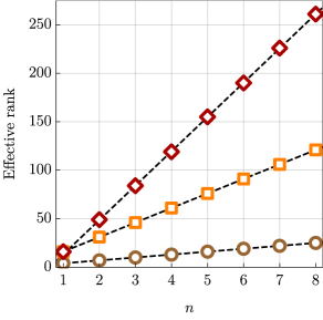
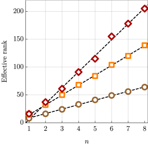
Figure 1: Effective rank of the $O^{ij}_{kl}$ intermediate for the linear alkanes C_nH_2n+2 (left panel) and water clusters $\big{(}$H₂O$\big{)}_{n}$ (right panel) extracted from the CCSD/cc-pVTZ calculations. The brown circles, orange squares and red diamonds indicate the effective rank obtained with the thresholds $\varepsilon=10^{-2}$, $10^{-3}$, and $10^{-4}$, respectively. The black dashed lines were obtained by least-squares fitting to the corresponding data points ($n=2,\ldots,8$).

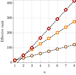
Figure 2: Effective rank of the $Z_{ij}^{ab}$ intermediate for the linear alkanes C_nH_2n+2 (left panel) and water clusters $\big{(}$H₂O$\big{)}_{n}$ (right panel) extracted from the CCSD/cc-pVTZ calculations. The brown circles, orange squares and red diamonds indicate the effective rank obtained with the thresholds $\varepsilon=10^{-3}$, $10^{-4}$, and $10^{-5}$, respectively. The black dashed lines were obtained by least-squares fitting to the corresponding data points ($n=2,\ldots,8$).

For both model systems we performed the exact CCSD calculations using the cc-pVTZ orbital basis setDunning (1989) and the corresponding cc-pVTZ-RIFIT density-fitting basisWeigend, Köhn, and Hättig (2002). The $1s$ core orbitals of carbon and oxygen atoms were frozen in these calculations. Next, we computed the $O^{ij}_{kl}$ and $Z_{ij}^{ab}$ intermediates with the converged doubly-excited amplitudes and performed the decompositions (25) and (26). Finally, for each system size $n$ and threshold value $\varepsilon$ we recorded the number of singular values (or absolute eigenvalues) larger than $\varepsilon$. This number is referred to further in the text as the effective rank. The results are illustrated in Fig. 1 for the $O^{ij}_{kl}$ intermediate and in Fig. 2 for the $Z_{ij}^{ab}$ intermediate. For the former quantity we considered the thresholds $\varepsilon=10^{-2}$, $10^{-3}$, and $10^{-4}$. For the latter we replaced $\varepsilon=10^{-2}$ by $\varepsilon=10^{-5}$ because the effective ranks for $\varepsilon=10^{-2}$ were too small ($\leq 6$) for a meaningful comparison. The results presented in Fig. 1 and Fig. 2 confirm the conjecture that the effective ranks of both intermediates increase only linearly with the system size. This statement is true to a good degree of approximation for every truncation threshold $\varepsilon$ considered here. Some deviations from the trend line are observed for the more challenging test case of water clusters, but only for the smallest value of the threshold ($\varepsilon=10^{-5}$). It is also noteworthy that a decrease of $\varepsilon$ by an order of magnitude leads to an increase of the slope of the linear trend line by approximately a factor of two.

To address the question whether the results represented graphically in Figs. 1 and 2 can be reproduced also in a smaller basis set, we performed analogous calculations with the cc-pVDZ basis. The plots of effective ranks analogous to Fig. 1 and 2 are given in supplementary material. In summary, the effective ranks change by no more than 5% when going from the cc-pVDZ to the cc-pVTZ basis. The only exception occurs for the water clusters with the smallest threshold ($\varepsilon=10^{-5}$), where the changes are slightly larger. Nonetheless, the linear growth of the effective ranks with the system size is confirmed in every case.

III.4 Quintic-scaling formulation

Having shown that the effective ranks of the $O^{ij}_{kl}$ and $Z_{ij}^{ab}$ intermediates increase only linearly (rather than quadratically) with the system size, we now describe how this observation can be exploited to decrease the scaling of the RR-CCSD calculations to the level of $N^{5}$. For simplicity, we consider the $O^{ij}_{kl}$ intermediate first; extension of this approach to $Z_{ij}^{ab}$ is presented further in the text.

In the modified RR-CCSD theory the $O^{ij}_{kl}$ intermediate is represented as

$$O^{ij}_{kl}=\alpha_{ik}^{F}\,o_{FG}\,\alpha_{jl}^{G},$$ (27)

The expansion vectors $\alpha_{ij}^{F}$ are obtained before the iterations and are fixed thereafter, while the core matrix $o_{FG}$ changes from iteration to iteration. The length of this expansion, i.e. the summations over $F$, $G$, is denoted $N_{\mathrm{O}}$ further in the text and it scales linearly with the system size. A suitable expansion basis $\alpha_{ik}^{F}$ is obtained by diagonalization of Eq. (25) reshaped as a symmetric $O^{2}\times O^{2}$ matrix $O_{ik,jl}$, and taking $N_{\mathrm{O}}$ eigenvectors that correspond to the largest absolute eigenvalues ($N_{\mathrm{O}}$ dominant eigenvectors). Because the exact CCSD amplitudes entering Eq. (25) are not known before the iterations, they are approximated by their MP2 or MP3 counterparts in the rank-reduced form

$$t_{ij}^{ab}=U_{ia}^{X}\;d_{X}\,U_{jb}^{X},$$ (28)

that are obtained according to the scheme presented in Sec. III.2. For brevity, we no longer distinguish the MP2 and MP3 amplitudes here [$t_{ij}^{ab}(\mbox{MP2})$ and $t_{ij}^{ab}(\mbox{MP3})$], because the treatment of the $O^{ij}_{kl}$ and $Z_{ij}^{ab}$ intermediates described below is the same in both cases.

Asymptotically, the $N_{\mathrm{O}}$ parameter is much smaller than the dimension ($O^{2}$) of the $O_{ik,jl}$ matrix. Therefore, the full diagonalization of the matrix $O_{ik,jl}$ can be avoided and only a subset of $N_{\mathrm{O}}$ dominant eigenpairs has to be found. This task can be accomplished efficiently ($N^{5}$ overall scaling) provided that the product $O^{ij}_{kl}\,q_{jl}$, where $q_{jl}$ is an arbitrary trial vector, can be calculated with $N^{4}$ cost. To prove that we first define an auxiliary quantity

$$B_{ki}^{QX}=B_{kc}^{Q}\,U_{ic}^{X},$$ (29)

which can be calculated before the diagonalization ($O^{2}VN_{\mathrm{aux}}N_{\mathrm{eig}}$ cost) and stored. Next, we combine the initial formula (25) with Eqs. (28) – (29) and rearrange the order of elementary operations as follows

$$O^{ij}_{kl}\,q_{jl}=B_{ki}^{QX}\Big{(}d_{X}\,B_{lj}^{QX}q_{jl}\Big{)}.$$ (30)

The $O^{2}N_{\mathrm{aux}}N_{\mathrm{eig}}\propto N^{4}$ cost of the two contraction steps becomes evident.

Because the expansion basis $\alpha_{ik}^{F}$ is fixed, in each RR-CCSD iteration one has to find an updated core matrix $o_{FG}$, taking into account that the compressed amplitudes $t_{XY}$ from Eq. (1) change. To simplify this task we note that as a byproduct of the diagonalization procedure, the expansion vectors obey the orthonormality relation $\alpha_{ij}^{F}\,\alpha_{ij}^{G}=\delta_{FG}$. Therefore, in every iteration the core matrix is given by an explicit expression

$$o_{FG}=\alpha_{ik}^{F}\,O^{ij}_{kl}\,\alpha_{jl}^{G}.$$ (31)

By using the definition (23) and inserting the formulas (28) and (29) we arrive at

$$o_{FG}=\Big{(}B_{ki}^{QX}\,\alpha_{ik}^{F}\Big{)}t_{XY}\,\Big{(}B_{lj}^{QY}\,\alpha_{jl}^{G}\Big{)}.$$ (32)

Finally, the contribution of the $O^{ij}_{kl}$ intermediate to the RR-CCSD residual is calculated by inserting Eqs. (27) into (22)

$$\frac{1}{2}\,P_{XY}\Big{[}\big{(}\alpha_{ik}^{F}\,U_{ka}^{Z}\,U_{ia}^{X}\big{)}o_{FG}\,t_{ZW}\big{(}\alpha_{jl}^{G}\,U_{lb}^{W}\,U_{jb}^{Y}\big{)}\Big{]}\rightarrow r_{XY}.$$ (33)

It is straightforward to show that both Eq. (32) and (33) can be evaluated with $N^{5}$ computational cost. Note that the quantity in the round brackets in Eq. (33) does not change during the RR-CCSD iterations and hence it can be precomputed and stored.

The treatment of the $Z_{ij}^{ab}$ intermediate is based on the following representation

$$Z_{ij}^{ab}=\beta_{ij}^{F}\,z_{FG}\,\beta_{ab}^{G}.$$ (34)

with the expansion length (denoted $N_{\mathrm{Z}}$) proportional to the system size. The expansion vectors $\beta_{ij}^{F}$ and $\beta_{ab}^{G}$ are obtained from SVD of Eq. (26) reshaped as a rectangular $O^{2}\times V^{2}$ matrix $Z_{ij,ab}$, taking $N_{\mathrm{Z}}$ left- and right-singular vectors corresponding to the largest singular values. Similarly as for the $O^{ij}_{kl}$ intermediate, MP2 or MP3 amplitudes are used in Eq. (26), so that the expansion vectors do not have to be updated in every RR-CCSD iteration. To guarantee that the SVD can be calculated efficiently, we consider the left-hand- and right-hand-side multiplications, $Z_{ij}^{ab}\,y_{ij}$ and $Z_{ij}^{ab}\,y_{ab}$, by an arbitrary pair of trial vectors, $y_{ij}$ and $y_{ab}$. The necessary factorized formulas read

$$Z_{ij}^{ab}\,y_{ij}=B_{kb}^{Q}\,U_{ka}^{X}\,\big{(}d_{X}\,B_{ij}^{QX}\,y_{ij}\big{)},$$ (35)

$$Z_{ij}^{ab}\,y_{ab}=B_{ij}^{QX}\,d_{X}\,\big{(}B_{kb}^{Q}\,U_{ka}^{X}\,y_{ab}\big{)}.$$ (36)

Each elementary contraction in the above formulas can be computed with $N^{4}$ cost. As a result, the overall computational cost of the truncated SVD (with the rank $N_{\mathrm{Z}}$) of the $Z_{ij}^{ab}$ intermediate scales as the fifth power of the system size.

During each RR-CCSD iteration the core matrix $z_{FG}$ is calculated from the explicit formula

$$z_{FG}=\big{(}\beta_{ij}^{F}\,B_{ij}^{QX}\,t_{XY}\big{)}\,\big{(}B_{kb}^{Q}\,U_{ka}^{Y}\,\beta_{ab}^{G}\big{)},$$ (37)

exploiting the orthonormality relations $\beta_{ij}^{F}\,\beta_{ij}^{G}=\delta_{FG}$ and $\beta_{ab}^{F}\,\beta_{ab}^{G}=\delta_{FG}$ which result from properties of singular value decomposition. Finally, the contribution to the residual is obtained from

$$\frac{1}{2}P_{XY}\Big{[}\big{(}\beta_{ki}^{F}\,U_{ka}^{Z}\,U_{ia}^{X}\big{)}\,t_{ZW}\,z_{FG}\,\big{(}U_{jc}^{W}\,\beta_{bc}^{G}\,U_{jb}^{Y}\big{)}\Big{]}\rightarrow r_{XY}.$$ (38)

The computational costs of evaluating the above expressions scale as $OVN_{\mathrm{aux}}N_{\mathrm{eig}}N_{\mathrm{Z}}\propto N^{5}$ and $OVN_{\mathrm{aux}}N_{\mathrm{eig}}^{2}\propto N^{5}$ in the rate determining steps. This proves that by exploiting the compressed formats of the intermediates (27) and (34), and noting their effective rank scales only linearly with the system size, the overall cost of RR-CCSD iterations can be reduced to the level of $N^{5}$.

The issue that has not been discussed yet is the practical choice of the expansion lengths in Eqs. (27) and (34), denoted by the symbols $N_{\mathrm{O}}$ and $N_{\mathrm{Z}}$. For convenience, we express both of them as multiples of the number of occupied orbitals in the system, i.e. $N_{\mathrm{O}}=mO$ and $N_{\mathrm{Z}}=m^{\prime}O$, where the parameters $m$ and $m^{\prime}$ are asymptotically independent of the system size. Clearly, the parameters $m$ and $m^{\prime}$ should be chosen to provide an optimal balance between the truncation error and the computational overhead of performing the decompositions (27) and (34). To recommend suitable value of $m$ and $m^{\prime}$ we require a larger and a more diverse test set of molecules than the model systems considered previously in the paper. For this purpose, we employ the Adler-Werner benchmark set developed in Ref. Adler and Werner, 2011. From this set we removed the hydrogen molecule as it is too small to be useful for the present purposes. This leaves $70$ molecules ranging in size from two to about twenty light atoms (H, C, N, O, S, Cl). The original geometries from Ref. Adler and Werner, 2011 were used throughout. The $1s$ core orbitals were frozen in all correlated calculations; for the second row atoms the $2s$ and $2p$ orbitals were also excluded.

For all molecules in the Adler-Werner benchmark set we performed two groups of RR-CCSD calculations, both within the cc-pVDZ orbital basis. In the first group adopted no approximations to the $O^{ij}_{kl}$ and $Z_{ij}^{ab}$ intermediates. Therefore, the scaling of these calculations is $N^{6}$ and their purpose is only to provide the reference results for a given $N_{\mathrm{eig}}$. In the second group of the RR-CCSD calculations we employ the decomposed form of the $O^{ij}_{kl}$ and $Z_{ij}^{ab}$ intermediates and hence the scaling is $N^{5}$, but the approximations (27) and (34) introduce an error. The magnitude of this error is quantified by comparing the corresponding results from the first and second group with the same $N_{\mathrm{eig}}$. This means that the error resulting from approximation of the doubly-excited amplitudes, Eq. (1), is not considered at this point. The only source of the error is the incompleteness of the representation of the $O^{ij}_{kl}$ and $Z_{ij}^{ab}$ intermediates themselves. The expansion lengths in Eqs. (27) and (34) are controlled by the parameters $N_{\mathrm{O}}$ and $N_{\mathrm{Z}}$ which, in general, can be varied completely independently. However, in our preliminary calculations we found that near-optimal results are obtained for equal values of these parameters, i.e. $N_{\mathrm{O}}=N_{\mathrm{Z}}$. Accuracy gains attainable by an independent adjustment of $N_{\mathrm{O}}$ and $N_{\mathrm{Z}}$ are not worth the corresponding increase of the complexity. Therefore, we set $N_{\mathrm{O}}=N_{\mathrm{Z}}$ (or $m=m^{\prime}$) from this point onward.

Table 1: Statistical measures of relative errors (in percent) in the RR-CCSD/cc-pVDZ correlation energy (for $N_{\mathrm{eig}}=N_{\mathrm{MO}}$) resulting from truncation of the expansions (27) and (34) at length $N_{\mathrm{O}}=N_{\mathrm{Z}}=mO$, where $O$ is the number of occupied orbitals in the system and the value of the parameter $m$ is given in the first column. The statistics comes from RR-CCSD/cc-pVDZ calculations for 70 molecules contained in the Adler-Werner benchmark set Adler and Werner (2011).

$m$	mean	mean abs.	standard	max. abs.
	error	error	deviation	error
$1$	$-0.167$	$0.168$	$0.043$	$0.340$
$2$	$-0.069$	$0.077$	$0.042$	$0.165$
$3$	$-0.032$	$0.037$	$0.022$	$0.066$
$4$	$-0.015$	$0.016$	$0.009$	$0.032$

Table 2: The same data as in Table 1, but for $N_{\mathrm{eig}}=2\cdot N_{\mathrm{MO}}$.

$m$	mean	mean abs.	standard	max. abs.
	error	error	deviation	error
$1$	$-0.169$	$0.169$	$0.046$	$0.321$
$2$	$-0.074$	$0.079$	$0.035$	$0.152$
$3$	$-0.034$	$0.042$	$0.028$	$0.097$
$4$	$-0.016$	$0.017$	$0.010$	$0.033$

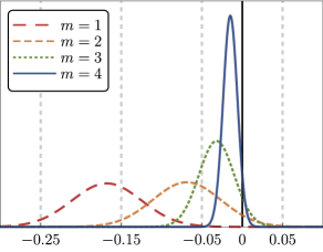
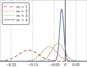
Figure 3: Distribution of relative error (in percent) resulting from the truncation of the expansions (27) and (34) at length $N_{\mathrm{O}}=N_{\mathrm{Z}}=mO$, where $O$ is the number of occupied orbitals in the system and the value of the parameter $m$ is given in the legend. The top and bottom panels correspond to $N_{\mathrm{eig}}=N_{\mathrm{MO}}$ and $N_{\mathrm{eig}}=2\cdot N_{\mathrm{MO}}$, respectively. The statistics comes from RR-CCSD/cc-pVDZ calculations for 70 molecules contained in the Adler-Werner benchmark set Adler and Werner (2011).

The calculations for the Alder-Werner benchmark set were performed for two representative examples of $N_{\mathrm{eig}}=N_{\mathrm{MO}}$ and $N_{\mathrm{eig}}=2\cdot N_{\mathrm{MO}}$, where $N_{\mathrm{MO}}$ is the total number of active orbitals in a given system (occupied plus virtual, neglecting the frozen-core orbitals). The expansion vectors $U_{ia}^{X}$ come from diagonalization of the MP2 amplitudes, but nearly the same results are obtained with the MP3 amplitudes. All data are given for $N_{\mathrm{O}}=N_{\mathrm{Z}}=mO$ with $m=1$, $2$, $3$, $4$. As the size of Alder-Werner benchmark set is substantial and comparison of individual results is cumbersome, we provide statistical error measures to access the quality of the results for each value of the control parameters $N_{\mathrm{O}}=N_{\mathrm{Z}}$. In Tables 1 and 2 we report such measures for relative errors in the RR-CCSD correlation energies: the mean relative error, mean absolute relative error, standard deviation of the relative error and maximum absolute relative error. Since the molecules included in the Alder-Werner set vary considerably in size, relative errors are preferred due to their size-intensive character. We found that for each value of the parameters $m$ and $N_{\mathrm{eig}}$ the distributions of the (signed) relative errors are well approximated by the normal (Gaussian) distribution with the mean and standard deviation indicated in Tables 1 and 2. In Fig. 3 we represent these distributions graphically to simplify the analysis of the results.

In general, the approximate treatment of the $O^{ij}_{kl}$ and $Z_{ij}^{ab}$ intermediates leads to minor errors in the RR-CCSD energy. Even with the smallest expansion length considered here ($N_{\mathrm{O}}=N_{\mathrm{Z}}=O$) more than 99.8% of the correlation energy is recovered. Beyond this point the error vanishes with increasing $N_{\mathrm{O}}$ and $N_{\mathrm{Z}}$ at a rate close to exponential; with $N_{\mathrm{O}}=N_{\mathrm{Z}}=4O$ the relative error decreases below 0.02%. Moreover, the error distributions for $N_{\mathrm{eig}}=N_{\mathrm{MO}}$ and $N_{\mathrm{eig}}=2\cdot N_{\mathrm{MO}}$ are remarkably similar, indicating that the truncation error of Eqs. (27) and (34) is practically independent of the dimension of the double excitation subspace. It is also noteworthy that the approximate treatment of the $O^{ij}_{kl}$ and $Z_{ij}^{ab}$ intermediates systematically underestimates the correlation energy. In summary, the results obtained with $N_{\mathrm{O}}=N_{\mathrm{Z}}=3O$ are, on average, sufficiently accurate for routine applications, with the mean error of only about 0.03%. However, the standard deviation of the error obtained with $N_{\mathrm{O}}=N_{\mathrm{Z}}=3O$ is still substantial compared to its mean, and hence the error distribution is rather broad. From the practical point of view, this negatively impacts the reliability of the method since it is not uncommon to encounter ”outliers“ with unexpectedly large errors. Therefore, we recommend that $N_{\mathrm{O}}=N_{\mathrm{Z}}=4O$ is used in actual applications where the reference results are not available. As is evident from Fig. 3 the error distribution for $N_{\mathrm{O}}=N_{\mathrm{Z}}=4O$ is much narrower than for $N_{\mathrm{O}}=N_{\mathrm{Z}}=3O$ which translates into a decreased likelihood of encountering the outliers. At the same time, the jump from $N_{\mathrm{O}}=N_{\mathrm{Z}}=3O$ to $N_{\mathrm{O}}=N_{\mathrm{Z}}=4O$ leads to only a minor increase of the overall computational timings. Therefore, all numerical results reported further in this work were obtained with $N_{\mathrm{O}}=N_{\mathrm{Z}}=4O$.

It is also important to study how the augmentation of the basis set with diffuse functions influences the accuracy of the approximations adopted for the $O^{ij}_{kl}$ and $Z_{ij}^{ab}$ intermediates. To address this question, we performed analogous calculations for the Alder-Werner benchmark set as described in the previous paragraph, but employing the aug-cc-pVDZ basis set Kendall, Dunning, and Harrison (1992). As the results are essentially insensitive to the value of the $N_{\mathrm{eig}}$ parameter, in supplementary material we report the data for the representative case of $N_{\mathrm{eig}}=N_{\mathrm{MO}}$. In summary, the augmentation of the basis set has a tiny influence on the accuracy of the decomposition applied to the $O^{ij}_{kl}$ and $Z_{ij}^{ab}$ intermediates. As an example, for the recommended expansion length ($N_{\mathrm{O}}=N_{\mathrm{Z}}=4O$) the mean relative error in the correlation energy increases only by about one thousandth of a percent upon the augmentation. Therefore, the approach proposed in the present work with the recommended expansion length ($N_{\mathrm{O}}=N_{\mathrm{Z}}=4O$) can be safely applied in calculations with diffuse basis set functions.

It is worthwhile to point out that there are two equivalent ways of selecting the dimension of the subspace used for the expansion of the $O^{ij}_{kl}$ and $Z_{ij}^{ab}$ intermediates. The first is to specify the values of parameters $N_{\mathrm{O}}$ and $N_{\mathrm{Z}}$ by relating it to another quantity that scales linearly with the system size, as was done in the calculations above ($N_{\mathrm{O}}=N_{\mathrm{Z}}=mO$). In this way the values of $N_{\mathrm{O}}$ and $N_{\mathrm{Z}}$ are known before the calculations are even started. However, an alternative idea is to form the subspace by taking all singular vectors with singular values larger than the predefined numerical threshold $\epsilon$. In other words, $N_{\mathrm{O}}$ and $N_{\mathrm{Z}}$ are found dynamically during the SVD procedure based on the parameter $\epsilon$ provided by the user. The main advantage of knowing $N_{\mathrm{O}}$ and $N_{\mathrm{Z}}$ in advance, besides the fact that the computational cost and scaling of the method can be judged more easily, is purely technical. In fact, implementation of an SVD procedure that dynamically adjusts the expansion length in each iteration is significantly more complicated than with fixed $N_{\mathrm{O}}$ and $N_{\mathrm{Z}}$, and can be expected to be also less efficient, especially in parallel environment. To address the question whether is worth the effort to develop an algorithm that dynamically adjusts the expansion length, we performed calculations for a subset of the Alder-Werner benchmark set. In the supplementary material we provide a comparison of the fixed and dynamic approach for one molecule we found representative of the whole set. As an example, the dynamic adjustment based on $\epsilon$ reduces the expansion length by about 15% if the relative accuracy of 99.95% is desired. While this reduction is non-negligible, this finding has to be understood in a broader context. In fact, in the next section we provide a comparison of timings of various steps of the RR-CCSD calculations. We show that the determination of the subspace used for the expansion of the $O^{ij}_{kl}$ and $Z_{ij}^{ab}$ intermediates constitutes less than 5% of the total RR-CCSD timings. Therefore, while the cost of handling the $O^{ij}_{kl}$ and $Z_{ij}^{ab}$ intermediates alone may be reduced using the dynamic adjustment of the expansion length, this would lead to only a minuscule decrease of the overall cost of the RR-CCSD method.

Finally, let us discuss how the approximations to the $O^{ij}_{kl}$ and $Z_{ij}^{ab}$ intermediates adopted in the present work affect the size-extensivity of the energy and how the present approach can be extended to calculation of, e.g. molecular properties. Similarly as discussed in Ref. Parrish et al., 2019, there are two necessary conditions that the expansion basis used in Eqs. (27) and (34) must fulfill. First, the basis vectors must be obtained using approximate doubly-excited amplitudes coming from a method that is size-extensive itself. In the present work MP2 or MP3 amplitudes are used which both fulfill this requirement. Second, the expansion length in Eqs. (27) and (34) must be a size-extensive quantity and hence increase linearly with the system size. We verified numerically using the model systems of linear alkanes and water clusters considered above, that the original Parrish et al. (2019) and the modified RR-CCSD variants retain the size-extensive property.

Moving on to the calculation of the RR-CCSD properties, in the original formulation of the RR-CCSD method described in Ref. Parrish et al., 2019, the projectors $U_{ia}^{X}$ are assumed to be perturbation-independent. Therefore, the Lagrangian formulation introduced in Ref. Parrish et al., 2019 enables straightforward calculation of molecular properties, using a similar approach as in the conventional coupled-cluster theory. It is reasonable to adopt the same condition for expansion basis in Eqs. (27) and (34) which leaves only the core matrices $o_{FG}$ and $z_{FG}$ as additional perturbation-dependent quantities whose response must be taken into account explicitly. In order to extend the RR-CCSD Lagrangian in this direction one requires to specify the stationary conditions that $o_{FG}$ and $z_{FG}$ fulfill. Taking the former matrix as an example, let us define the following quantity

$$\tau=\sum_{ijkl}\Big{[}O^{ij}_{kl}-\sum_{FG}\alpha_{ik}^{F}\,o_{FG}\,\alpha_{jl}^{G}\Big{]}.$$ (39)

One can show that at convergence of the RR-CCSD iterations this quantity is stationary with respect to $o_{FG}$ in the sense that $\frac{\partial\tau}{\partial o_{FG}}=0$ as this condition becomes equivalent to Eq. (32). Therefore, the modified RR-CCSD Lagrangian is defined by adding a term $\zeta_{FG}\,\frac{\partial\tau}{\partial o_{FG}}$, where $\zeta_{FG}$ is a new set of Lagrange multipliers. By minimization of this modified Lagrangian with respect to all perturbation-dependent parameters ($t_{XY}$, $o_{FG}$) one obtains equations that have to be solved to find the multipliers. As a result, the Lagrangian is stationary with respect to all parameters which enables straightforward determination of molecular properties using the extended Hellmann-Feynman theorem.

III.5 Accuracy and efficiency of the method

Table 3: Statistical measures of relative errors (in percent) in the RR-CCSD correlation energy with respect to the exact CCSD results. The dimension of the excitation subspace ($N_{\mathrm{eig}}$) is expressed as $N_{\mathrm{eig}}=x\cdot N_{\mathrm{MO}}$, where $N_{\mathrm{MO}}$ is the total number of orbitals in the system. The subspace of double excitations was obtained by diagonalization of MP2 amplitudes. The statistics comes from calculations for 70 molecules contained in the Adler-Werner benchmark set Adler and Werner (2011).

$x$	mean	mean abs.	standard	max. abs.
	error	error	deviation	error
cc-pVDZ basis set
$0.5$	0.349	0.365	0.310	1.419
$1.0$	0.608	0.608	0.268	2.034
$1.5$	0.285	0.290	0.128	0.538
$2.0$	0.197	0.203	0.118	0.427
$2.5$	0.227	0.228	0.195	1.601
cc-pVTZ basis set
$0.5$	0.342	0.343	0.164	1.275
$1.0$	0.309	0.312	0.140	1.124
$1.5$	0.088	0.119	0.113	0.333
$2.0$	0.106	0.124	0.149	0.300
$2.5$	0.123	0.131	0.079	0.259

Table 4: The same data as in Table 3, but the subspace of double excitations was obtained by diagonalization of MP3 amplitudes.

$x$	mean	mean abs.	standard	max. abs.
	error	error	deviation	error
cc-pVDZ basis set
$0.5$	0.100	0.286	0.371	1.128
$1.0$	0.468	0.468	0.216	2.053
$1.5$	0.294	0.294	0.081	0.487
$2.0$	0.158	0.158	0.052	0.298
$2.5$	0.068	0.069	0.034	0.223
cc-pVTZ basis set
$0.5$	$-$0.203	0.257	0.165	0.917
$1.0$	$-$0.259	0.258	0.143	1.372
$1.5$	$-$0.121	0.121	0.044	0.422
$2.0$	$-$0.037	0.039	0.027	0.114
$2.5$	$-$0.004	0.018	0.024	0.076

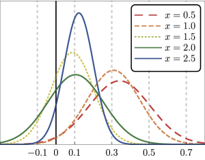
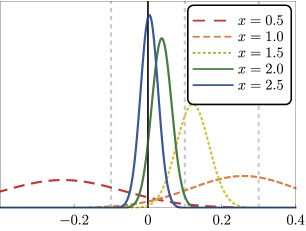
Figure 4: Distribution of relative error (in percent) in the RR-CCSD/cc-pVTZ correlation energy with respect to the exact CCSD/cc-pVTZ results. The dimension of the excitation subspace ($N_{\mathrm{eig}}$) is expressed as $N_{\mathrm{eig}}=x\cdot N_{\mathrm{MO}}$, where $N_{\mathrm{MO}}$ is the total number of orbitals in the system. The excitations subspace was obtained by diagonalization of MP2 amplitudes (top panel) or MP3 amplitudes (bottom panel). The statistics comes from calculations for 70 molecules contained in the Adler-Werner benchmark set Adler and Werner (2011). See the supplementary material for analogous results obtained within cc-pVDZ basis set.

In this section we study the cumulative error of the RR-CCSD method incurred by the truncation of the double excitation subspace (as a function of $N_{\mathrm{eig}}$) and the approximate treatment of the $O^{ij}_{kl}$ and $Z_{ij}^{ab}$ intermediates. In contrast to Sec. III.4, the exact CCSD correlation energies obtained within the same basis set are treated as a reference here. The RR-CCSD calculations for the whole Alder-Werner benchmark set were performed with $N_{\mathrm{eig}}=x\cdot N_{\mathrm{MO}}$, where $x$ is a parameter taking values $x=0.50$, $1.00$, $1.50$, $2.00$, $2.50$, and with the recommended $N_{\mathrm{O}}=N_{\mathrm{Z}}=4O$. All calculations were performed within the cc-pVDZ and cc-pVTZ basis sets. We consider two variants of the method, where the subspace of double excitations is obtained by diagonalization of either MP2 or MP3 amplitudes. Statistical measures of relative errors in the RR-CCSD correlation energy with respect to the exact CCSD results for both variants are given in Tables 3 and 4. Similarly as in the previous section, we found that the corresponding error distributions are approximately normal and are given in Fig. 4 in the case of the cc-pVTZ basis set. For brevity, plots representing analogous results obtained within the cc-pVDZ basis were moved to the supplementary material.

From Tables 3 and 4 one concludes that the MP2 excitation subspace is not well-suited for highly accurate calculation of the correlation energy. While for smaller values of $N_{\mathrm{eig}}$ ($x=0.5-1.0$) the MP2 basis performs only marginally worse than MP3, for larger $x$ the former method stalls in terms of relative accuracy at the level of $0.2-0.3\%$ in the cc-pVDZ basis and $0.1-0.2\%$ in the cc-pVTZ basis. If errors of this magnitude are acceptable, the MP2 basis is a reasonable choice due to the marginal cost of its determination. However, it is uneconomical to aim at the accuracy levels of $0.1\%$ or better with the MP2 basis, as the error decays too slowly as a function of $N_{\mathrm{eig}}$. As a result, in accurate calculations where relative errors below $0.1\%$ are expected, MP3 amplitudes are necessary. The MP3 basis does not suffer from the diminishing returns as $N_{\mathrm{eig}}$ is increased, and the convergence with respect to $N_{\mathrm{eig}}$ is fast even in the high-accuracy regime. For $N_{\mathrm{eig}}=2N_{\mathrm{MO}}$ the MP3 basis achieves relative accuracy of about $0.1\%$ in the cc-pVDZ basis and about $0.04\%$ in the cc-pVTZ basis. As a side note, this demonstrates that the amplitudes obtained within the larger basis set are more ”compressible“ and we expect this phenomenon to prevail as the basis set is increased further. To sum up, we recommend that $N_{\mathrm{eig}}=2N_{\mathrm{MO}}$ is used to fix the expansion length in Eq. (1), both in the case of MP2 and MP3 excitation bases. This value strikes a balance between the computational cost of the RR-CCSD procedure and the accuracy level it offers.

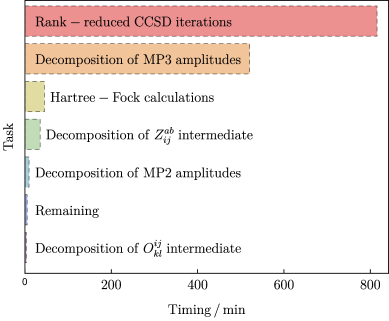
Figure 5: Breakdown of the RR-CCSD/cc-pVTZ wall clock timings for the ethylbenzene molecule (C₈H₁₀, 380 molecular orbitals). The timings of the Hartree-Fock calculations are given for comparison (default Gamess settings, density matrix convergence threshold $10^{-8}$). The category ”remaining“ includes minor tasks such as updating the coupled-cluster amplitudes, evaluating the energy, etc. The calculations were performed using a single core of AMD Opteron™  Processor 6174 (no parallelization).

To study the computational efficiency of the RR-CCSD method we first analyze which steps of the RR-CCSD algorithm bring the dominant contribution to the total timings. To this end, we consider the largest molecule in the Adler-Werner set (ethylbenzene, C₈H₁₀) employing the cc-pVTZ basis set (380 molecular orbitals). We employ the recommended values of the truncation parameters, namely $N_{\mathrm{eig}}=2N_{\mathrm{MO}}$, $N_{\mathrm{O}}=N_{\mathrm{Z}}=4O$. In Fig. 5 we present a breakdown of the total RR-CCSD wall clock timings into individual components of the algorithm. For comparison, timings of the Hartree-Fock calculations obtained with the default Gamess settings and the density matrix convergence threshold of $10^{-8}$ are also given. From Fig. 5 it is clear that two steps of the proposed RR-CCSD algorithm, namely diagonalization of the MP2 amplitudes and decomposition of the $O^{ij}_{kl}$ intermediate, are essentially negligible in terms of the computational effort. The treatment of $Z_{ij}^{ab}$ intermediate is somewhat more costly, but still comparable with the conventional Hartree-Fock calculations. Therefore, while the decomposition of the $O^{ij}_{kl}$ and $Z_{ij}^{ab}$ intermediates advocated in this work scales formally as $N^{5}$ with the system size, the prefactor of this procedure is small and hence this step does not contribute significantly to the overall workload. On the other hand, the diagonalization of the MP3 amplitudes introduces a considerable overhead. With the current implementation the total costs of finding the MP3 excitation subspace and the subsequent RR-CCSD iterations are comparable.

In general, the pilot implementation of the RR-CCSD method reported in this paper is limited to $600-700$ basis set functions, but this limitation results from overuse of disk files for storage of intermediate quantities. We are currently working on an improved implementation that avoids this problem and hence should vastly exceed the capabilities of the conventional CCSD implementations. In fact, shortly after the present manuscript was submitted for publication, another article was published hohenstein21a that describes a GPU-accelerated parallel implementation of the RR-CCSD method applicable up to ca. 2000 basis set functions. Notably, this was achieved without any special treatment of the non-factorizable terms in the RR-CCSD residual, and hence the implementation reported in Ref. hohenstein21a scales as $N^{6}$. Because of that, the non-factorizable terms turned out to be the bottleneck of this implementation for large systems. Clearly, an efficient implementation of the RR-CCSD method with the treatment of the non-factorizable terms described in the present work should be capable of reaching even larger systems. An alternative method of eliminating the non-factorizable terms based on the tensor hypercontraction (THC) decomposition of the doubly-excited amplitudes has also been reported recently hohenstein21b.

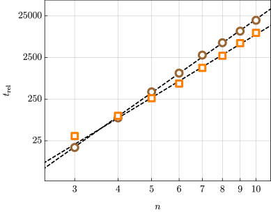
Figure 6: Timings of the RR-CCSD/cc-pVDZ calculations with $N_{\mathrm{eig}}=2N_{\mathrm{MO}}$, $N_{\mathrm{O}}=N_{\mathrm{Z}}=4O$ (orange squares) and of the exact CCSD/cc-pVDZ calculations (brown circles) for linear alkanes C_nH_2n+2 as a function of the chain length, $n$ (logarithmic scale on both axes). The timings are given in relation to the CCSD calculations for methane ($t_{\mathrm{rel}}$). The calculations were performed using a single core of AMD Opteron™  Processor 6174 (no parallelization). The black dashed lines were obtained by least-squares fitting of the data points with the functional form $a\cdot n^{b}$ (represented by linear functions on doubly-logarithmic scale).

Finally, to compare the performance of the RR-CCSD and the exact CCSD methods, we analyze their timings for the linear alkanes C_nH_2n+2 previously considered in Sec. III.3. In Fig. 6 we report the total wall clock times of the CCSD and RR-CCSD calculations (cc-pVDZ basis set) as a function of the alkanes chain length, $n$. Similarly as above, we employ the recommended values of the truncation parameters, namely $N_{\mathrm{eig}}=2N_{\mathrm{MO}}$, $N_{\mathrm{O}}=N_{\mathrm{Z}}=4O$. The timings for the RR-CCSD method include determination of the double-excitation subspace, treatment of the $O^{ij}_{kl}$ and $Z_{ij}^{ab}$ intermediates and all other steps discussed in the previous paragraph. To convert the data into dimensionless units the timings are given in relation to the CCSD calculations for methane.

To confirm numerically that the scaling observed in Fig. 6 matches the theoretical predictions from Sec. III.4 we fitted the timings with the functional form $a\cdot n^{b}$ for $n=3-10$. We obtained the exponents $b=5.04$ for the RR-CCSD method and $5.86$ for the exact CCSD theory, in a good agreement with the conclusions of Sec. III.4. Another important issue is to estimate for how large systems the RR-CCSD method becomes advantageous in terms of computational timings. From Fig. 6 we see that the break-even point for linear alkanes occurs rather early, around $n=4$ (butane). Beyond this point the RR-CCSD is less computationally expensive, with the gap increasing linearly with the molecular size. For the fixed values of the control parameters ($N_{\mathrm{eig}}=2N_{\mathrm{MO}}$, $N_{\mathrm{O}}$, and $N_{\mathrm{Z}}$) we expect this finding to be approximately valid also for other systems, with the break-even point occurring for about thirty or so active electrons.

IV Perturbative triples corrections

IV.1 Problem formulation

It is well-known that the conventional coupled-cluster theory with only single and double excitations included in the cluster operator is insufficient to obtain chemically-accurate predictions. In fact, only after triple excitations are accounted for, levels of accuracy of 1 kcal/mol or better become routinely accessibleBartlett et al. (1990); Hopkins and Tschumper (2004); Bak et al. (2000); Tajti et al. (2004); Karton et al. (2006); Riley et al. (2010). However, the computational cost of the coupled-cluster theory with full inclusion of triple excitations is prohibitively high for systems comprising more than a few non-hydrogen atoms. For this reason, numerous approximate schemes were proposed to account for the effects of triple excitations in a more affordable way without sacrificing too much accuracy. The most widely-used method of this type is the CCSD(T) theory of Raghavachari et al.Raghavachari et al. (1989), frequently referred to as the ”gold standard“ of quantum chemistry.

The CCSD(T) theory is perturbative in nature and adds a non-iterative correction, denoted shortly $E_{\mathrm{(T)}}$ further in the text, on top of the standard CCSD energy. This correction is a sum of two terms

$$E_{\mathrm{(T)}}=E_{\mathrm{T}}^{[4]}+E_{\mathrm{ST}}^{[5]}$$ (40)

defined as

$$E_{\mathrm{T}}^{[4]}=\langle T_{2}^{\mathrm{SD}}|\Big{[}W,T_{3}\Big{]}\rangle,$$ (41)

and

$$E_{\mathrm{ST}}^{[5]}=\langle T_{1}^{\mathrm{SD}}|\Big{[}W,T_{3}\Big{]}\rangle,$$ (42)

where $T_{1}^{\mathrm{SD}}$ and $T_{2}^{\mathrm{SD}}$ is an abbreviation for cluster operators (7) obtained at the CCSD level of theory. The triple excitation operator present in Eqs. (40) and (41) is given by the standard formula

$$T_{3}=\frac{1}{6}\,t_{ijk}^{abc}\,E_{ai}\,E_{bj}\,E_{ck},$$ (43)

where the amplitudes $t_{ijk}^{abc}$ are approximated as

$$t_{ijk}^{abc}\approx(\epsilon_{ijk}^{abc})^{-1}\,\Gamma_{ijk}^{abc},$$ (44)

$$\Gamma_{ijk}^{abc}=\langle\,_{ijk}^{abc}|\big{[}W,T_{2}^{\mathrm{SD}}\big{]}\rangle,$$ (45)

and $\epsilon_{ijk}^{abc}=\epsilon_{i}^{a}+\epsilon_{j}^{b}+\epsilon_{k}^{c}$ is the three-particle energy denominator. The evaluation of the corrections $E_{\mathrm{T}}^{[4]}$ and $E_{\mathrm{ST}}^{[5]}$ scales as $N^{7}$ with the system size, if no further approximations are introduced.

A natural extension of the RR-CCSD method is to evaluate the $E_{\mathrm{(T)}}$ correction with the singly- and doubly-excited amplitudes obtained within the rank-reduced formalism and add it to the RR-CCSD correlation energy. The resulting method is abbreviated RR-CCSD(T) further in the paper and we expect it to faithfully reproduce the exact CCSD(T) results. Unfortunately, the steep $N^{7}$ scaling of the $E_{\mathrm{(T)}}$ correction would constitute a severe bottleneck in applications to larger systems, in comparison to the more subdued $N^{5}$ cost of the RR-CCSD iterations. To the best of our knowledge, the $N^{7}$ scaling cannot be reduced by exploiting solely the rank-reduced form of the $T_{2}^{\mathrm{SD}}$ amplitudes given by Eq. (1). Therefore, additional approximations are needed to make the RR-CCSD(T) method advantageous which is explored in the subsequent section.

IV.2 Compression of the triply excited amplitudes

To decrease the scaling of the $E_{\mathrm{(T)}}$ correction removal of the three-particle energy denominator from Eq. (44) is a priority. To this end, we employ the same min-max quadrature as in Sec. III.2 for the MP2 and MP3 amplitudes. The Laplace transformation formula now reads

$$(\epsilon_{ijk}^{abc})^{-1}=w_{g}\,e^{-t_{g}\big{(}\epsilon_{i}^{a}+\epsilon_{j}^{b}+\epsilon_{k}^{c}\big{)}},$$ (46)

where the notation for all quantities in the same as in Sec. III.2. As demonstrated in the paper of Constans et al.Constans, Ayala, and Scuseria (2000) application of the Laplace transformation of the three-particle energy denominator alone is sufficient to reduce the scaling of the $E_{\mathrm{T}}^{[4]}$ and $E_{\mathrm{ST}}^{[5]}$ terms to the level of $N^{6}$. Unfortunately, the subsequent factorization yields numerous terms with a large prefactor ($OV^{5}$ scaling) and hence the computational benefits are achieved only for very large systems. To avoid this problem, in Ref. Constans, Ayala, and Scuseria, 2000 the $E_{\mathrm{T}}^{[4]}$ and $E_{\mathrm{ST}}^{[5]}$ corrections were rewritten in terms of CCSD natural orbitals, enabling an efficient screening procedure to eliminate negligible contributions. Here we propose an alternative approach where the triply-excited amplitudes (44) are approximately represented in the Tucker-3 formatTucker (1966)

$$t_{ijk}^{abc}=t_{ABC}\,V_{ia}^{A}\,V_{jb}^{B}\,V_{kc}^{C}.$$ (47)

In analogy to Eq. (1) the basis vectors $V_{ia}^{A}$ span the subspace of triple excitations. The dimension of this subspace, i.e. the length of the summations over the variables $A$, $B$, $C$ in Eq. (47), is denoted $N_{\mathrm{trip}}$ further in the paper. Note that the Tucker-3 decomposition has been recently applied to the full CCSDT methodLesiuk (2020a) with the quantities $V_{ia}^{A}$ obtained by higher-order singular value decompositionDe Lathauwer, De Moor, and Vandewalle (2000a); Vannieuwenhoven, Vandebril, and Meerbergen (2012) (HOSVD) of Eq. (44). More importantly, it has also been shown that $N_{\mathrm{trip}}$ has to scale only linearly with the system size in order to maintain a constant relative accuracy in the correlation energy. As demonstrated further in the text, this allows to calculate the $E_{\mathrm{T}}^{[4]}$ and $E_{\mathrm{ST}}^{[5]}$ corrections with the cost proportional to $N^{6}$ and an acceptable prefactor. Unfortunately, the HOSVD method adopted in Ref. Lesiuk, 2020a is not feasible in the present context due to a prohibitive cost. To achieve the decomposition (47) we thus employ a variant of the higher-order orthogonal iteration (HOOI) procedureDe Lathauwer, De Moor, and Vandewalle (2000b); Eldén and Savas (2009) which is a particular method of minimizing the least-squares error

$$\tau=\sum_{ijk}\sum_{abc}\bigg{[}t_{ijk}^{abc}-t_{ABC}\,V_{ia}^{A}\,V_{jb}^{B}\,V_{kc}^{C}\bigg{]}^{2},$$ (48)

subject to the orthonormality condition $V_{ia}^{A}\,V_{ia}^{B}=\delta_{AB}$. While HOOI is a well-known tool in the mathematics literature, we are aware of only one paper where it is used in the context of the electronic structure theoryBell, Lambrecht, and Head-Gordon (2010).

To apply the HOOI procedure to the $t_{ijk}^{abc}$ amplitudes one requires an initial guess of the basis vectors $V_{ia}^{A}$. In our implementation this guess is generated by taking the basis vectors $U_{ia}^{X}$ (obtained previously for the doubly-excited amplitudes) that correspond to the largest absolute eigenvalues. While a more sophisticated and effective guess can definitely be proposed, we found this simple and self-contained approach to be entirely adequate. The HOOI procedure consists of two basic steps

• evaluate the partially contracted quantity

  $$t_{ia,BC}=t_{ijk}^{abc}\,V_{jb}^{B}\,V_{kc}^{C},$$ (49)

  with current estimation of the factors $V_{ia}^{A}$;

• compute SVD of $t_{ia,BC}$ reshaped as a $OV\times N_{\mathrm{trip}}^{2}$ matrix and take left-singular vectors that correspond to the largest singular values as the next $V_{ia}^{A}$.

These steps are repeated until convergence; the choice of the stopping criteria is discussed further in the text. The computational costs of both steps scale as the fifth power of the system size. This is straightforward to prove in the case of the second step by noting that we need to find only a subset of $N_{\mathrm{trip}}$ singular vectors with the largest singular values. As $N_{\mathrm{trip}}$ is proportional to the system size, application of the decomposition algorithm described in Sec. II.3 immediately results in $N^{5}$ cost. The first step of the HOOI algorithm can also be accomplished with the same scaling. To show that we recall the explicit formula for the quantity $\Gamma_{ijk}^{abc}$ defined in Eq. (44):

$$\begin{split}\Gamma_{ijk}^{abc}&=\Big{(}1+P_{jk}^{bc}\Big{)}\Big{(}1+P_{ij}^{ab}+P_{ik}^{ac}\Big{)}\\ &\times\Big{[}t_{ij}^{ad}\,(ck|bd)-t_{il}^{ab}\,(ck|lj)\Big{]},\end{split}$$ (50)

By inserting the density-fitting form of the two-electron integrals together with the decomposed amplitudes (1) and defining the intermediate

$$\bar{D}_{jb}^{QX}=\Big{(}B_{bd}^{Q}\,U_{jd}^{Y}-B_{lj}^{Q}\,U_{lb}^{Y}\Big{)}\,t_{XY},$$ (51)

we bring Eq. (50) into a simpler form

$$\Gamma_{ijk}^{abc} =\Big{(}1+P_{jk}^{bc}\Big{)}\Big{(}1+P_{ij}^{ab}+P_{ik}^{ac}\Big{)}U_{ia}^{X}\,\bar{D}_{jb}^{QX}\,B_{kc}^{Q}.$$ (52)

This leads to the working expression for the partially contracted quantity $t_{ia,BC}$ required in the HOOI algorithm

$$\begin{split}t_{ia,BC}&=\big{(}1+P_{BC}\big{)}w_{g}\,e^{-t_{g}\epsilon_{i}^{a}}\\ &\times\Big{[}U_{ia}^{X}\,\Big{(}\bar{D}_{jb}^{QX}\,V_{jb}^{B}\,e^{-t_{g}\epsilon_{j}^{b}}\Big{)}\Big{(}B_{kc}^{Q}\,V_{kc}^{C}\,e^{-t_{g}\epsilon_{k}^{c}}\Big{)}\\ &+\,\bar{D}_{ia}^{QX}\,\Big{(}U_{jb}^{X}\,V_{jb}^{B}\,e^{-t_{g}\epsilon_{j}^{b}}\Big{)}\Big{(}B_{kc}^{Q}\,V_{kc}^{C}\,e^{-t_{g}\epsilon_{k}^{c}}\Big{)}\\ &+\,B_{ia}^{Q}\,\Big{(}U_{jb}^{X}\,V_{jb}^{B}\,e^{-t_{g}\epsilon_{j}^{b}}\Big{)}\Big{(}\bar{D}_{kc}^{QX}\,V_{kc}^{C}\,e^{-t_{g}\epsilon_{k}^{c}}\Big{)}\Big{]}.\end{split}$$ (53)

It is straightforward to verify that each elementary contraction in the above formula involves at most five indices at the same time, not including the Laplace grid index. As a result, the cost of assembling the quantity $t_{ia,BC}$ scales as the fifth power of the system size.

Finally, we discuss the issue of the stopping criteria in the HOOI procedure. The obvious choices are to monitor either the least-squares error of Eq. (47) or the norm of the difference between $V_{ia}^{A}$ obtained in two subsequent iterations. Unfortunately, both of these ideas are troublesome in practice. The calculation of the least-squares error during every HOOI iteration is prohibitively expensive as it involves quantities such as $\Big{(}t_{ijk}^{abc}\Big{)}^{2}$. The use of the differences between the expansion vectors $V^{A}_{ai}$ is not effective due to non-uniqueness of the singular vectors which may change from iteration to iteration without affecting the error in Eq. (47).

To avoid these problems, we monitor the norm of the core tensor $t_{ABC}$ as a proxy for the convergence of the procedure, namely

$$||t||^{2}=\sum_{ABC}t_{ABC}^{2}=\sum_{ABC}\Big{(}\sum_{ia}t_{ia,BC}\,V_{ia}^{A}\Big{)}\Big{(}\sum_{jb}t_{jb,BC}\,V_{jb}^{A}\Big{)},$$ (54)

where summation symbols were added for clarity. The second equality is a consequence of the orthonormality of the $V^{A}_{ai}$ vectors obtained from the SVD procedure. The HOOI procedure is terminated when the difference in $||t||$ between two consecutive iterations falls below a predefined threshold. The threshold value $10^{-5}$ is sufficient in most applications and has been adopted in the present work. The cost of computing $||t||$ during every iteration is negligible in comparison with other parts of the algorithm as $t_{ia,BC}$ is explicitly available anyway. The reason why this simplified procedure is adequate follows from the fact that the HOOI algorithm can be equivalently formulated as a maximization of the norm of the core tensor rather than the minimization of the least-squares error as in Eq. (48), see Refs. Kolda and Bader, 2009 and reference therein.

With the triply-excited amplitudes represented in the rank-reduced format (47), the remaining task is to evaluate the $E_{\mathrm{T}}^{[4]}$ and $E_{\mathrm{ST}}^{[5]}$ corrections. Derivation of explicit formulas for these corrections given in terms of basic two-electron integrals and cluster amplitudes is straightforward, but the resulting expressions are rather lengthy. Therefore, they are given in the full form in the supplementary material. However, it is worth pointing out that the $E_{\mathrm{ST}}^{[5]}$ correction is expressed as a sum of four distinct terms with the computational complexity of $N^{5}$ or lower. Assuming that $N_{\mathrm{aux}}>N_{\mathrm{trip}}$, the most expensive of them scales as $O^{2}N_{\mathrm{aux}}N_{\mathrm{trip}}^{2}$ or $O^{2}VN_{\mathrm{aux}}N_{\mathrm{trip}}$ depending on the ratio of $V$ to $N_{\mathrm{trip}}$. Explicit formula for $E_{\mathrm{T}}^{[4]}$ comprises six terms, the most expensive two scaling as $O^{2}VN_{\mathrm{eig}}N_{\mathrm{aux}}N_{\mathrm{trip}}\propto N^{6}$. Therefore, evaluation of the $E_{\mathrm{(T)}}$ correction in the rank-reduced formalism possesses $N^{6}$ computational complexity, lower than the $O^{3}V^{4}\propto N^{7}$ scaling of the conventional algorithms. A rough estimate of the crossover point between two algorithms is obtained by recalling that $N_{\mathrm{eig}}\approx 2N_{\mathrm{MO}}\approx 2V$ is sufficient in practice in the RR-CCSD method, and that $N_{\mathrm{aux}}\approx 2-4V$ with the standard auxiliary basis sets. Therefore, even in the most computationally demanding scenario where $N_{\mathrm{trip}}\approx N_{\mathrm{eig}}$ is needed to achieve sufficient levels of accuracy, the crossover point occurs for relatively small systems with $O\approx 10$ or so.

IV.3 Accuracy of the RR-CCSD(T) method: total energies

Table 5: Statistical measures of relative errors (in percent) in the $E_{\mathrm{(T)}}$ correction in the rank-reduced formulation with respect to the exact results. The dimension of the triple excitation subspace ($N_{\mathrm{trip}}$) is expressed as $N_{\mathrm{trip}}=y\cdot N_{\mathrm{MO}}$, where $N_{\mathrm{MO}}$ is the total number of orbitals in the system. The statistics comes from calculations for 70 molecules contained in the Adler-Werner benchmark set Adler and Werner (2011).

$y$	mean	mean abs.	standard	max. abs.
	error	error	deviation	error
cc-pVDZ basis set
$0.50$	$-$16.63	16.65	5.81	25.00
$0.75$	0$-$7.33	07.71	4.34	14.42
$1.00$	0$-$2.89	03.76	3.17	07.37
$1.25$	0$-$1.58	02.57	2.59	05.65
$1.50$	0$-$0.71	01.88	2.19	05.19
cc-pVTZ basis set
$0.50$	$-$6.86	7.38	4.17	12.67
$0.75$	$-$1.89	2.79	2.75	6.93
$1.00$	$-$0.53	1.67	2.04	5.26
$1.25$	$-$0.31	1.21	1.49	4.64
$1.50$	$-$0.34	0.94	1.17	4.90

Table 6: The same data as in Table 5, except relative errors (in percent) in the total RR-CCSD(T) correlation energies are given.

$y$	mean	mean abs.	standard	max. abs.
	error	error	deviation	error
cc-pVDZ basis set
$0.50$	$-$0.397	0.411	0.240	0.900
$0.75$	$-$0.094	0.159	0.180	0.506
$1.00$	$-$0.053	0.099	0.133	0.534
$1.25$	$-$0.096	0.114	0.119	0.580
$1.50$	$-$0.125	0.130	0.107	0.591
cc-pVTZ basis set
$0.50$	$-$0.257	0.320	0.273	1.200
$0.75$	$-$0.041	0.136	0.210	1.269
$1.00$	$-$0.022	0.101	0.187	1.001
$1.25$	$-$0.034	0.083	0.171	0.871
$1.50$	$-$0.033	0.070	0.166	0.784

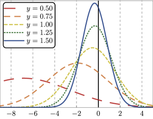
Figure 7: Distribution of relative error (in percent) in the $E_{\mathrm{(T)}}$ correction with respect to the exact results (cc-pVTZ basis). The dimension of the triples excitation subspace ($N_{\mathrm{trip}}$) is expressed as $N_{\mathrm{trip}}=y\cdot N_{\mathrm{MO}}$, where $N_{\mathrm{MO}}$ is the total number of orbitals in the system. The statistics comes from calculations for 70 molecules contained in the Adler-Werner benchmark set Adler and Werner (2011). See the supplementary material for analogous results obtained within the cc-pVDZ basis set.

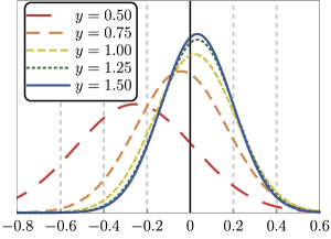
Figure 8: Distribution of relative error (in percent) in the total RR-CCSD(T)/cc-pVTZ correlation energy with respect to the exact CCSD(T)/cc-pVTZ method. The dimension of the triples excitation subspace ($N_{\mathrm{trip}}$) is expressed as $N_{\mathrm{trip}}=y\cdot N_{\mathrm{MO}}$, where $N_{\mathrm{MO}}$ is the total number of orbitals in the system. The statistics comes from calculations for 70 molecules contained in the Adler-Werner benchmark set Adler and Werner (2011). See the supplementary material for analogous results obtained within the cc-pVDZ basis set.

In order to study the accuracy levels that can realistically be reached with the RR-CCSD(T) method and find the value of the parameter $N_{\mathrm{trip}}$ that offers a compromise between accuracy and computational costs under typical conditions, we performed RR-CCSD(T) calculations for the Alder-Werner benchmark set. The other numerical parameters present in the RR-CCSD(T) method were fixed at their recommended values ($N_{\mathrm{eig}}=2N_{\mathrm{MO}}$ and $N_{\mathrm{O}}=N_{\mathrm{Z}}=4O$), so that the focus is solely on the remaining $N_{\mathrm{trip}}$ parameter. Additionally, in this section we consider only the RR-CCSD(T) method with the double excitation subspace obtained by diagonalization of the MP3 amplitudes. We found that the $E_{\mathrm{(T)}}$ correction, in contrast to the RR-CCSD energy, is rather insensitive to whether MP2 or MP3 amplitudes are used, with relative errors of the $E_{\mathrm{(T)}}$ correction differing by just a small fraction of a percent.

For each member of the Alder-Werner set we performed RR-CCSD(T) calculations with $N_{\mathrm{trip}}=y\cdot N_{\mathrm{MO}}$, where $y=0.50$, $0.75$, $1.00$, $1.25$, and $1.50$. Note that the $y$ parameter is asymptotically independent of the system size and hence we expect it to possess some universal value that delivers a decent accuracy in the $E_{\mathrm{(T)}}$ correction for a broad range of systems.

We aim at relative accuracy level of a few percent in the $E_{\mathrm{(T)}}$ correction. This is a reasonable target from the practical point of view, because $E_{\mathrm{(T)}}$ rarely contributes from the 5% of the total correlation energy in well-behaved systems. In Table 5 we report error statistics for the calculations of the $E_{\mathrm{(T)}}$ correction in the rank-reduced formulation. Analogous data are given also in Table 6, but there we consider errors in the total RR-CCSD(T) correlation energies, i.e. the sum of the RR-CCSD and $E_{\mathrm{(T)}}$ contributions, taking the exact CCSD(T) results as a reference. For ease of comparison, the distributions of errors for the $E_{\mathrm{(T)}}$ correction alone and for the total RR-CCSD(T) correlation energy (both within the cc-pVTZ basis set) are represented graphically in terms of normal distributions in Figs. 7 and 8, respectively. Analogous plots obtained with RR-CCSD(T)/cc-pVDZ method are given in the supplementary material.

The results reported in Fig. 7 reveal the overall trend in the accuracy of the $E_{\mathrm{(T)}}$ correction as a function of the $y$ parameter. Even with the smallest triple excitation subspace dimension considered here ($y=0.50$) a reasonable relative accuracy of several percent is obtained. This improves to about 0.5% when the parameter $y$ is increased to unity. Beyond the point $y=1$ the improvement rate slows down considerably. We verified that this phenomenon is a consequence of finite accuracy of the doubly-excited amplitudes (with the recommended $N_{\mathrm{eig}}=2N_{\mathrm{MO}}$) which limit the accuracy of the $E_{\mathrm{(T)}}$ correction for $y>1$.

Based on the results reported in Table 5, we recommend that for $N_{\mathrm{eig}}=2N_{\mathrm{MO}}$ the dimension of the triple-excitation subspace is set to $N_{\mathrm{trip}}=N_{\mathrm{MO}}$, corresponding to $y=1$. For this value of the parameter the accuracy of the $E_{\mathrm{(T)}}$ correction meets the criteria discussed in the previous paragraphs. Moreover, this choice is supported by the observation that a further increase of the parameter $y$ leads to minor improvements in the accuracy of the total RR-CCSD(T) energies, see Table 6. This is a result of an accidental, yet systematic cancellation of errors that occurs for $N_{\mathrm{eig}}=2N_{\mathrm{MO}}$ and $N_{\mathrm{trip}}=N_{\mathrm{MO}}$ where the RR-CCSD component of the energy is slightly underestimated, while the $E_{\mathrm{(T)}}$ correction is overestimated by a comparable amount. However, we verified that even in the absence of this fruitful error cancellation, i.e. assuming that both errors are of the same sign, the combination of the parameters $N_{\mathrm{eig}}=2N_{\mathrm{MO}}$ and $N_{\mathrm{trip}}=N_{\mathrm{MO}}$ would still provide accuracy levels better than 0.1% in the total RR-CCSD(T) energies. Therefore, the choice $N_{\mathrm{eig}}=2N_{\mathrm{MO}}$ and $N_{\mathrm{trip}}=N_{\mathrm{MO}}$ is both safe and pragmatic, and is adopted further in the paper.

IV.4 Accuracy of the RR-CCSD(T) method: relative energies

Finally, we study the accuracy of the RR-CCSD(T) method in reproduction of relative energies and compare the results with the reference CCSD(T) data. As the first test we employ the benchmark set of 34 isomerization energies of organic molecules introduced by Grimme et al.Grimme, Steinmetz, and Korth (2007) (usually abbreviated as ISO34 in the literature). The range of isomerization energies included in the ISO34 set spans from a few kJ/mol to a few hundreds kJ/mol. The RR-CCSD(T) calculations were performed with the recommended settings ($N_{\mathrm{eig}}=2N_{\mathrm{MO}}$, $N_{\mathrm{O}}=N_{\mathrm{Z}}=4O$, and $N_{\mathrm{trip}}=N_{\mathrm{MO}}$) and are compared with the exact CCSD(T) results obtained with NWChem package. Note that in the latter calculations we do not apply the density-fitting approximation of the two-electron integrals and hence the error budget of the RR-CCSD(T) results formally includes also the density-fitting error. In all calculations we employ the cc-pVTZ basis set and the $1s$ core orbitals of the first-row atoms were frozen. Within this setup the largest system included in the ISO34 set contains about 500 orbitals and 50 active electrons which is near the edge of applicability of the canonical CCSD(T) theory without further approximations or a parallelization.

Raw isomerization energies computed using the RR-CCSD(T) and the exact CCSD(T) methods are listed in the supplementary material. To simplify the analysis we consider statistical error measures with respect to the reference CCSD(T) method evaluated for the whole ISO34 set. The RR-CCSD(T)/cc-pVTZ method exhibits the mean error of $-$0.03 kJ/mol and mean absolute error of 0.32 kJ/mol. The standard deviation of the error equals to 0.38 kJ/mol. This level of accuracy is sufficient for many applications involving polyatomic molecules. Moreover, it is worth pointing out that the RR-CCSD(T) method is systematically improvable without a drastic increase of the computational costs. Therefore, if accuracy levels of, e.g., 0.1 kJ/mol are needed in a particular application, this requirement can be met by increasing the control parameters $N_{\mathrm{eig}}$ and $N_{\mathrm{trip}}$ above the values recommended currently.

The maximum absolute deviation among the isomerization energies from the ISO34 set was found for reaction 13 (styrene $\rightarrow$ cyclooctatetraene) and amounts to 0.77 kJ/mol. However, it has to be pointed out that the total isomerization energy for this reaction is particularly large (152.89 kJ/mol), so the relative error obtained in this case (about 0.5%) is still acceptable. At the same time, the RR-CCSD(T) method accurately reproduces also small energy differences, indicating a systematic error cancellation. For example, consider the smallest two isomerization energies from the ISO34 benchmark set equal to 4.66 kJ/mol and 4.73 kJ/mol for reaction 4 (trans-2-butene $\rightarrow$ cis-2-butene) and reaction 5 (isobutylene $\rightarrow$ trans-2-butene). The errors of the RR-CCSD(T) method for these reactions amount to $-$0.03 kJ/mol and $-$0.06 kJ/mol, respectively. This shows that the proposed method is capable of providing uniformly reliable results in a chemically-relevant energy range.

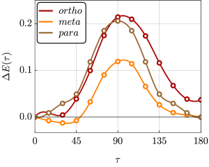
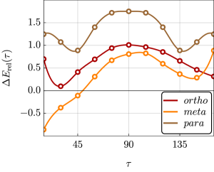
Figure 9: Absolute errors (left panel) and percent relative errors (right panel) in the RR-CCSD(T)/cc-pVTZ torsional energy curves for the ortho-, meta- and para-fluorophenols. The exact CCSD(T)/cc-pVTZ results are used as a reference.

The second group of model systems we employ to study the accuracy of the RR-CCSD(T) method in reproduction of relative energies are ortho-, meta- and para-fluorophenols. These systems have been intensively studied in the literature due to their rich microwave spectrum prototypical for hydrogen bond interactions with fluorineLarsen and Nicolaisen (1974); Larsen (1986); Smeyers and Hernández-Laguna (1987); Ratzer, Nispel, and Schmitt (2003); Jaman (2007); Bell et al. (2017). Here we consider the torsional energy differences related to the internal rotation of the hydroxyl moiety in relation to the plane of the aromatic ring. The torsional angle, denoted $\tau$ further in the text, is defined by the following sequence of four atoms: the hydrogen of the hydroxyl group, the oxygen, the carbon atom closest to the oxygen, and the next carbon atom in the ring closest to the fluorine atom (in the case of para-fluorophenol the last choice is arbitrary). By convention, in the case of ortho and meta isomers the torsional angle $\tau=0$ corresponds to the trans structure with the maximum distance between the hydrogen of the hydroxyl group and the fluorine atom.

Table 7: Parameters of the torsional energy curve (see the text for definitions of all quantities) for three isomers of fluorophenol computed using the RR-CCSD(T)/cc-pVTZ method (“RR”) and the exact CCSD(T)/cc-pVTZ method (“exact”). For each isomer relative energies with respect to its $\tau=0$ conformation are given. The angles are given in degrees and the energies in kJ/mol.

	ortho		meta		para
quantity	RR	exact	RR	exact	RR	exact
$\Delta E_{\mathrm{barrier}}$	021.62	021.84	14.63	14.75	11.55	11.76
$\tau_{\mathrm{barrier}}$	101.34	101.24	91.18	91.26	90.00	90.00
$\Delta E_{\mathrm{cis/trans}}$	011.36	011.40	$-$0.53	$-$0.53	00.00	00.00

We performed an energy scan varying the torsional angle $\tau$ from $0^{\circ}$ to $180^{\circ}$ in steps of $15^{\circ}$. The rest of the molecular geometry was fully optimized for each $\tau$ at the MP2/cc-pVTZ level of theory. Cartesian coordinates of the optimized structures are included in the supplementary material. Finally, the RR-CCSD(T)/cc-pVTZ and the exact CCSD(T)/cc-pVTZ calculations are performed on every optimized geometry with the same settings as for the ISO34 benchmark set. For each isomer, the $\tau=0$ conformation is treated as the zero-energy point and all other energies are given relative to it. In Fig. 9 we provide errors of the RR-CCSD(T)/cc-pVTZ torsional energies with respect to the exact CCSD(T)/cc-pVTZ for each isomer of the fluorophenol. Raw energies used to compile this plot are given in the supplementary material. From Fig. 9 it is clear that the errors in the torsional energies vary smoothly with $\tau$, without major jumps and discontinuities. The mean absolute errors (averaged over $\tau=15^{\circ},\ldots,180^{\circ}$) are $0.091\,/\,0.038\,/\,0.076$ kJ/mol for the ortho/meta/para isomers, while the corresponding standard deviations are $0.079\,/\,0.044\,/\,0.077$ kJ/mol. To further study the performance of the RR-CCSD(T) method we calculated three parameters that characterize the potential energy curves for each isomer:

• the height of the potential energy barrier separating the trans ($\tau=0$) and cis ($\tau=180^{\circ}$) conformations, $\Delta E_{\mathrm{barrier}}$;

• the value of the torsional angle corresponding to the maximum of the barrier, $\tau_{\mathrm{barrier}}$;

• the energy difference between the trans and cis conformations, $\Delta E_{\mathrm{trans/cis}}$.

The first two parameters were found with the help of $B$-splines interpolation of the calculated data points, followed by application of the Brent algorithmBrent (1971) to find the minimum of the interpolated curve. The numerical errors caused by this procedure are essentially negligible. The parameters $\Delta E_{\mathrm{barrier}}$, $\tau_{\mathrm{barrier}}$, and $\Delta E_{\mathrm{trans/cis}}$ determined for three conformers are reported in Table 7 and compared with the reference CCSD(T) values. The error of determining the barrier height is around 0.2 kJ/mol for each conformer, while the error of determining its location is below 0.1 degrees. In many applications to polyatomic molecules errors of this magnitude would be negligible in comparison with other uncertainties, such as the basis set incompleteness.

V Conclusions

In this work we have modified and extended the rank-reduced CCSD theory introduced by Parrish and collaborators with three major contributions. First, we have shown how a subset of eigenvectors of the MP2 and MP3 amplitudes, serving as the the expansion basis for the doubly-excited amplitudes in the RR-CCSD method, can be obtained efficiently with $N^{5}$ scaling. Second, we have eliminated the issue of non-factorizable terms from the RR-CCSD residual. We have provided a systematic way to approximate these terms using the singular value decomposition and reduced the overall scaling of the RR-CCSD iterations down to the level of $N^{5}$. Finally, we have considered the evaluation of the perturbative corrections to the CCSD energies resulting from triply excited configurations. The triply-excited amplitudes present in the CCSD(T) method have been decomposed to the Tucker-3 format using the higher-order orthogonal iteration (HOOI) procedure. This has enabled to compute the energy correction due to triple excitations non-iteratively with $N^{6}$ cost.

The accuracy of the proposed RR-CCSD(T) method in reproduction of total correlation energies has been studied using a diverse set of 70 polyatomic molecules comprising first- and second-row atoms. It has been shown that with the recommended values of the control parameters, relative accuracy levels better than 99.9% have been achieved, both in the double- and triple-zeta basis sets. Next, we have considered the accuracy of relative energies calculated with the RR-CCSD(T) method. Numerical results for isomerization energies of 34 organic molecules and conformational energies of substituted phenols have shown that average absolute errors are of the order of $0.1-0.3$ kJ/mol. Moreover, the calculated energy surfaces show no discontinuities and are suitable for fitting with a properly chosen functional form, which is usually a necessary step in nuclear dynamics simulations, for example. We have also compared efficiency of the reduced scaling RR-CCSD implementation with the standard CCSD algorithm. While we have shown that the break-even point beyond which the RR formulation becomes advantageous occurs for only $30-40$ active electrons, an efficient parallelized code is required to compete with carefully-optimized implementations reported recently that scale favorably to thousands of cores.

Finally, we point out possible extensions of the present work which are of particular interest. First, the rank-reduction concepts can be applied to the symmetry-adapted perturbation theory (SAPT)Jeziorski, Moszynski, and Szalewicz (1994); Hohenstein and Sherrill ; Szalewicz (2012); Jansen (2014). Higher-level variants of SAPTParker et al. (2014), such as SAPT2+ and SAPT2+(3), share a structure similar to the CCD theory with the exception that the excitation subspace for the supermolecule is formed as a union of excitations localized on the monomers. Another promising idea is to extend the rank-reduced formalism to the time-dependent coupled-cluster theoryHuber and Klamroth (2011); Kvaal (2012); Sato et al. (2018), where the high cost of the calculations is one of the main stumbling blocks that prevent routine applications to polyatomic molecules. Indeed, the computational effort of a single time step is usually comparable to several standard CC iterationsPedersen and Kvaal (2019); Kristiansen et al. (2020) and tens of thousands of time steps may be needed in simulations in strong laser fields. The applicability of the rank-reduced formalism to the time-dependent problems shall be the subject of a future study.

Supplementary Material

See supplementary material for additional numerical results obtained using the RR-CCSD and RR-CCSD(T) methods, tests of accuracy of the Laplace quadrature, and explicit analytical formulas for the factorizable terms in the RR-CCSD residual and for the $E_{\mathrm{T}}^{[4]}$ and $E_{\mathrm{ST}}^{[5]}$ corrections within the rank-reduced framework.

Data Availability Statement

The data that support the findings of this study are available within the article and its supplementary material.

References

- Crawford and Schaefer III (2007) T. D. Crawford and H. F. Schaefer III, “An introduction to coupled cluster theory for computational chemists,” in Reviews in Computational Chemistry (John Wiley & Sons, Ltd, 2007) pp. 33–136.
- Bartlett and Musiał (2007) R. J. Bartlett and M. Musiał, Rev. Mod. Phys. 79, 291 (2007).
- Raghavachari et al. (1989) K. Raghavachari, G. W. Trucks, J. A. Pople, and M. Head-Gordon, Chem. Phys. Lett. 157, 479 (1989).
- Kobayashi and Rendell (1997) R. Kobayashi and A. P. Rendell, Chem. Phys. Lett. 265, 1 (1997).
- Hirata (2003) S. Hirata, The Journal of Physical Chemistry A 107, 9887 (2003), https://doi.org/10.1021/jp034596z .
- Auer et al. (2006) A. A. Auer, G. Baumgartner, D. E. Bernholdt, A. Bibireata, V. Choppella, D. Cociorva, X. Gao, R. Harrison, S. Krishnamoorthy, S. Krishnan, C.-C. Lam, Q. Lu, M. Nooijen, R. Pitzer, J. Ramanujam, P. Sadayappan, and A. Sibiryakov, Molecular Physics 104, 211 (2006), https://doi.org/10.1080/00268970500275780 .
- Olson et al. (2007) R. M. Olson, J. L. Bentz, R. A. Kendall, M. W. Schmidt, and M. S. Gordon, J. Chem. Theory Comp. 3, 1312 (2007).
- Janowski, Ford, and Pulay (2007) T. Janowski, A. R. Ford, and P. Pulay, J. Chem. Theory Comp. 3, 1368 (2007).
- Janowski and Pulay (2008) T. Janowski and P. Pulay, J. Chem. Theory Comp. 4, 1585 (2008).
- van Dam et al. (2011) H. van Dam, W. de Jong, E. Bylaska, N. Govind, K. Kowalski, T. Straatsma, and M. Valiev, WIREs Computational Molecular Science 1, 888 (2011), https://wires.onlinelibrary.wiley.com/doi/pdf/10.1002/wcms.62 .
- Deumens et al. (2011) E. Deumens, V. F. Lotrich, A. Perera, M. J. Ponton, B. A. Sanders, and R. J. Bartlett, WIREs Comput. Mol. Sci. 1, 895 (2011).
- Anisimov et al. (2014) V. M. Anisimov, G. H. Bauer, K. Chadalavada, R. M. Olson, J. W. Glenski, W. T. C. Kramer, E. Aprà, and K. Kowalski, J. Chem. Theory Comp. 10, 4307 (2014).
- Solomonik et al. (2014) E. Solomonik, D. Matthews, J. R. Hammond, J. F. Stanton, and J. Demmel, J. Parallel Distr. Comp. 74, 3176 (2014).
- Calvin, Lewis, and Valeev (2015) J. A. Calvin, C. A. Lewis, and E. F. Valeev, in Proceedings of the 5th Workshop on Irregular Applications: Architectures and Algorithms, IA3 ’15 (Association for Computing Machinery, New York, NY, USA, 2015).
- Peng et al. (2016) C. Peng, J. A. Calvin, F. Pavošević, J. Zhang, and E. F. Valeev, The Journal of Physical Chemistry A 120, 10231 (2016), pMID: 27966947, https://doi.org/10.1021/acs.jpca.6b10150 .
- Lyakh (2019) D. I. Lyakh, International Journal of Quantum Chemistry 119, e25926 (2019), https://onlinelibrary.wiley.com/doi/pdf/10.1002/qua.25926 .
- Gyevi-Nagy, Kállay, and Nagy (2020) L. Gyevi-Nagy, M. Kállay, and P. R. Nagy, J. Chem. Theory Comp. 16, 366 (2020).
- Peng et al. (2020) C. Peng, C. A. Lewis, X. Wang, M. C. Clement, K. Pierce, V. Rishi, F. Pavošević, S. Slattery, J. Zhang, N. Teke, A. Kumar, C. Masteran, A. Asadchev, J. A. Calvin, and E. F. Valeev, The Journal of Chemical Physics 153, 044120 (2020), https://doi.org/10.1063/5.0005889 .
- Datta and Gordon (2021) D. Datta and M. S. Gordon, J. Chem. Theory Comp. 17, 4799 (2021).
- Gyevi-Nagy, Kállay, and Nagy (2021) L. Gyevi-Nagy, M. Kállay, and P. R. Nagy, J. Chem. Theory Comp. 17, 860 (2021).
- Kowalski et al. (2021) K. Kowalski, R. Bair, N. P. Bauman, J. S. Boschen, E. J. Bylaska, J. Daily, W. A. de Jong, T. Dunning, N. Govind, R. J. Harrison, M. Keçeli, K. Keipert, S. Krishnamoorthy, S. Kumar, E. Mutlu, B. Palmer, A. Panyala, B. Peng, R. M. Richard, T. P. Straatsma, P. Sushko, E. F. Valeev, M. Valiev, H. J. J. van Dam, J. M. Waldrop, D. B. Williams-Young, C. Yang, M. Zalewski, and T. L. Windus, Chemical Reviews 121, 4962 (2021), pMID: 33788546, https://doi.org/10.1021/acs.chemrev.0c00998 .
- Calvin et al. (2021) J. A. Calvin, C. Peng, V. Rishi, A. Kumar, and E. F. Valeev, Chemical Reviews 121, 1203 (2021), pMID: 33305957, https://doi.org/10.1021/acs.chemrev.0c00006 .
- DePrince and Hammond (2011) A. E. DePrince and J. R. Hammond, J. Chem. Theory Comp. 7, 1287 (2011).
- Ma et al. (2011) W. Ma, S. Krishnamoorthy, O. Villa, and K. Kowalski, J. Chem. Theory Comp. 7, 1316 (2011).
- A. Eugene DePrince et al. (2014) I. A. Eugene DePrince, M. R. Kennedy, B. G. Sumpter, and C. D. Sherrill, Mol. Phys. 112, 844 (2014).
- Kaliman and Krylov (2017) I. A. Kaliman and A. I. Krylov, J. Comp. Chem. 38, 842 (2017).
- DePrince III, Hammond, and Sherrill (2016) A. E. DePrince III, J. R. Hammond, and C. D. Sherrill, “Iterative coupled-cluster methods on graphics processing units,” in Electronic Structure Calculations on Graphics Processing Units (John Wiley & Sons, Ltd, 2016) Chap. 13, pp. 279–300.
- Peng, Calvin, and Valeev (2019) C. Peng, J. A. Calvin, and E. F. Valeev, Int. J. Quantum Chem. 119, e25894 (2019).
- Wang, Guo, and Wang (2020) Z. Wang, M. Guo, and F. Wang, Phys. Chem. Chem. Phys. 22, 25103 (2020).
- Seritan et al. (2020) S. Seritan, C. Bannwarth, B. S. Fales, E. G. Hohenstein, S. I. L. Kokkila-Schumacher, N. Luehr, J. W. Snyder, C. Song, A. V. Titov, I. S. Ufimtsev, and T. J. Martínez, J. Chem. Phys. 152, 224110 (2020).
- Adamowicz and Bartlett (1987) L. Adamowicz and R. J. Bartlett, J. Chem. Phys. 86, 6314 (1987).
- Adamowicz, Bartlett, and Sadlej (1988) L. Adamowicz, R. J. Bartlett, and A. J. Sadlej, J. Chem. Phys. 88, 5749 (1988).
- Neogrády, Pitoňák, and Urban (2005) P. Neogrády, M. Pitoňák, and M. Urban, Mol. Phys. 103, 2141 (2005).
- Pitoňák et al. (2006) M. Pitoňák, F. Holka, P. Neogrády, and M. Urban, J. Mol. Struct. 768, 79 (2006).
- Kumar and Crawford (2017) A. Kumar and T. D. Crawford, The Journal of Physical Chemistry A 121, 708 (2017), pMID: 28045265, https://doi.org/10.1021/acs.jpca.6b11410 .
- Yang et al. (2011) J. Yang, Y. Kurashige, F. R. Manby, and G. K. L. Chan, J. Chem. Phys. 134, 044123 (2011).
- Kurashige et al. (2012) Y. Kurashige, J. Yang, G. K.-L. Chan, and F. R. Manby, J. Chem. Phys. 136, 124106 (2012).
- Yang et al. (2012) J. Yang, G. K.-L. Chan, F. R. Manby, M. Schütz, and H.-J. Werner, J. Chem. Phys. 136, 144105 (2012).
- Schütz et al. (2013) M. Schütz, J. Yang, G. K.-L. Chan, F. R. Manby, and H.-J. Werner, J. Chem. Phys. 138, 054109 (2013).
- Li, Ma, and Jiang (2002) S. Li, J. Ma, and Y. Jiang, Journal of Computational Chemistry 23, 237 (2002), https://onlinelibrary.wiley.com/doi/pdf/10.1002/jcc.10003 .
- Li et al. (2006) S. Li, J. Shen, W. Li, and Y. Jiang, The Journal of Chemical Physics 125, 074109 (2006), https://doi.org/10.1063/1.2244566 .
- Li et al. (2009) W. Li, P. Piecuch, J. R. Gour, and S. Li, The Journal of Chemical Physics 131, 114109 (2009), https://doi.org/10.1063/1.3218842 .
- Neese, Wennmohs, and Hansen (2009) F. Neese, F. Wennmohs, and A. Hansen, J. Chem. Phys. 130, 114108 (2009).
- Li and Piecuch (2010a) W. Li and P. Piecuch, The Journal of Physical Chemistry A 114, 6721 (2010a), pMID: 20496942, https://doi.org/10.1021/jp1038738 .
- Li and Piecuch (2010b) W. Li and P. Piecuch, The Journal of Physical Chemistry A 114, 8644 (2010b), pMID: 20373794, https://doi.org/10.1021/jp100782u .
- Rolik and Kállay (2011) Z. Rolik and M. Kállay, The Journal of Chemical Physics 135, 104111 (2011), https://doi.org/10.1063/1.3632085 .
- Rolik et al. (2013) Z. Rolik, L. Szegedy, I. Ladjánszki, B. Ladóczki, and M. Kállay, The Journal of Chemical Physics 139, 094105 (2013), https://doi.org/10.1063/1.4819401 .
- Riplinger and Neese (2013) C. Riplinger and F. Neese, J. Chem. Phys. 138, 034106 (2013).
- Riplinger et al. (2013) C. Riplinger, B. Sandhoefer, A. Hansen, and F. Neese, J. Chem. Phys. 139, 134101 (2013).
- Liakos et al. (2015) D. G. Liakos, M. Sparta, M. K. Kesharwani, J. M. L. Martin, and F. Neese, J. Chem. Theory Comput. 11, 1525 (2015).
- Schwilk et al. (2017) M. Schwilk, Q. Ma, C. Köppl, and H.-J. Werner, J. Chem. Theory Comput. 13, 3650 (2017).
- Kolda and Bader (2009) T. G. Kolda and B. W. Bader, SIAM Rev. 51, 455 (2009).
- Whitten (1973) J. L. Whitten, J. Chem. Phys. 58, 4496 (1973).
- Baerends, Ellis, and Ros (1973) E. Baerends, D. Ellis, and P. Ros, Chem. Phys. 2, 41 (1973).
- Dunlap, Connolly, and Sabin (1979) B. I. Dunlap, J. W. D. Connolly, and J. R. Sabin, J. Chem. Phys. 71, 3396 (1979).
- Van Alsenoy (1988) C. Van Alsenoy, J. Comp. Chem. 9, 620 (1988).
- Vahtras, Almlöf, and Feyereisen (1993) O. Vahtras, J. Almlöf, and M. Feyereisen, Chem. Phys. Lett. 213, 514 (1993).
- Beebe and Linderberg (1997) N. H. F. Beebe and J. Linderberg, Int. J. Quantum Chem. 12, 683 (1997).
- Koch, Sánchez de Merás, and Pedersen (2003) H. Koch, A. Sánchez de Merás, and T. B. Pedersen, J. Chem. Phys. 118, 9481 (2003).
- Pedersen, Sánchez de Merás, and Koch (2004) T. B. Pedersen, A. M. J. Sánchez de Merás, and H. Koch, J. Chem. Phys. 120, 8887 (2004).
- Folkestad, Kjønstad, and Koch (2019) S. D. Folkestad, E. F. Kjønstad, and H. Koch, J. Chem. Phys. 150, 194112 (2019).
- Martinez, Mehta, and Carter (1992) T. J. Martinez, A. Mehta, and E. A. Carter, The Journal of Chemical Physics 97, 1876 (1992), https://doi.org/10.1063/1.463176 .
- Martinez and Carter (1993) T. J. Martinez and E. A. Carter, The Journal of Chemical Physics 98, 7081 (1993), https://doi.org/10.1063/1.464751 .
- Martinez and Carter (1994) T. J. Martinez and E. A. Carter, The Journal of Chemical Physics 100, 3631 (1994), https://doi.org/10.1063/1.466350 .
- Martinez and Carter (1995) T. J. Martinez and E. A. Carter, The Journal of Chemical Physics 102, 7564 (1995), https://doi.org/10.1063/1.469088 .
- Reynolds, Martinez, and Carter (1996) G. Reynolds, T. J. Martinez, and E. A. Carter, The Journal of Chemical Physics 105, 6455 (1996), https://doi.org/10.1063/1.472495 .
- Neese et al. (2009) F. Neese, F. Wennmohs, A. Hansen, and U. Becker, Chem. Phys. 356, 98 (2009).
- Kossmann and Neese (2010) S. Kossmann and F. Neese, J. Chem. Theory Comput. 6, 2325 (2010).
- Izsák and Neese (2011) R. Izsák and F. Neese, J. Chem. Phys. 135, 144105 (2011).
- Petrenko, Kossmann, and Neese (2011) T. Petrenko, S. Kossmann, and F. Neese, J. Chem. Phys. 134, 054116 (2011).
- Izsák, Hansen, and Neese (2012) R. Izsák, A. Hansen, and F. Neese, Mol. Phys. 110, 2413 (2012).
- Izsák and Neese (2013) R. Izsák and F. Neese, Mol. Phys. 111, 1190 (2013).
- Dutta, Neese, and Izsák (2016) A. K. Dutta, F. Neese, and R. Izsák, J. Chem. Phys. 144, 034102 (2016).
- Hohenstein, Parrish, and Martínez (2012) E. G. Hohenstein, R. M. Parrish, and T. J. Martínez, The Journal of Chemical Physics 137, 044103 (2012), https://doi.org/10.1063/1.4732310 .
- Parrish et al. (2012) R. M. Parrish, E. G. Hohenstein, T. J. Martínez, and C. D. Sherrill, J. Chem. Phys. 137, 224106 (2012).
- Parrish et al. (2013a) R. M. Parrish, E. G. Hohenstein, N. F. Schunck, C. D. Sherrill, and T. J. Martínez, Phys. Rev. Lett. 111, 132505 (2013a).
- Parrish et al. (2013b) R. M. Parrish, E. G. Hohenstein, T. J. Martínez, and C. D. Sherrill, J. Chem. Phys. 138, 194107 (2013b).
- Benedikt et al. (2011) U. Benedikt, A. A. Auer, M. Espig, and W. Hackbusch, J. Chem. Phys. 134, 054118 (2011).
- Benedikt, Böhm, and Auer (2013) U. Benedikt, K.-H. Böhm, and A. A. Auer, J. Chem. Phys. 139, 224101 (2013).
- Hohenstein et al. (2013a) E. G. Hohenstein, S. I. L. Kokkila, R. M. Parrish, and T. J. Martínez, J. Chem. Phys. 138, 124111 (2013a).
- Kokkila Schumacher et al. (2015) S. I. L. Kokkila Schumacher, E. G. Hohenstein, R. M. Parrish, L.-P. Wang, and T. J. Martínez, J. Chem. Theory Comput. 11, 3042 (2015).
- Lee, Lin, and Head-Gordon (2020) J. Lee, L. Lin, and M. Head-Gordon, J. Chem. Theory Comput. 16, 243 (2020).
- Matthews (2021) D. A. Matthews, J. Chem. Phys. 154, 134102 (2021).
- Bell, Lambrecht, and Head-Gordon (2010) F. Bell, D. Lambrecht, and M. Head-Gordon, Mol. Phys. 108, 2759 (2010).
- Kinoshita, Hino, and Bartlett (2003) T. Kinoshita, O. Hino, and R. J. Bartlett, J. Chem. Phys. 119, 7756 (2003).
- Hino, Kinoshita, and Bartlett (2004) O. Hino, T. Kinoshita, and R. J. Bartlett, J. Chem. Phys. 121, 1206 (2004).
- Scuseria, Henderson, and Sorensen (2008) G. E. Scuseria, T. M. Henderson, and D. C. Sorensen, J. Chem. Phys. 129, 231101 (2008).
- Schutski et al. (2017) R. Schutski, J. Zhao, T. M. Henderson, and G. E. Scuseria, The Journal of Chemical Physics 147, 184113 (2017), https://doi.org/10.1063/1.4996988 .
- Hohenstein et al. (2012) E. G. Hohenstein, R. M. Parrish, C. D. Sherrill, and T. J. Martínez, J. Chem. Phys. 137, 221101 (2012).
- Hohenstein et al. (2013b) E. G. Hohenstein, S. I. L. Kokkila, R. M. Parrish, and T. J. Martínez, J. Phys. Chem. B 117, 12972 (2013b).
- Parrish et al. (2014) R. M. Parrish, C. D. Sherrill, E. G. Hohenstein, S. I. L. Kokkila, and T. J. Martínez, J. Chem. Phys. 140, 181102 (2014).
- Lesiuk (2020a) M. Lesiuk, J. Chem. Theory Comput. 16, 453 (2020a).
- Parrish et al. (2019) R. M. Parrish, Y. Zhao, E. G. Hohenstein, and T. J. Martínez, J. Chem. Phys. 150, 164118 (2019).
- Helgaker et al. (1997) T. Helgaker, W. Klopper, H. Koch, and J. Noga, J. Chem. Phys. 106, 9639 (1997).
- Karton, Taylor, and Martin (2007) A. Karton, P. R. Taylor, and J. M. L. Martin, J. Chem. Phys. 127, 064104 (2007).
- Martin and de Oliveira (1999) J. M. L. Martin and G. de Oliveira, J. Chem. Phys. 111, 1843 (1999).
- Tucker (1966) L. R. Tucker, Psychometrika 31, 279 (1966).
- Lesiuk (2019) M. Lesiuk, J. Comp. Chem. 40, 1319 (2019).
- De Lathauwer, De Moor, and Vandewalle (2000a) L. De Lathauwer, B. De Moor, and J. Vandewalle, SIAM J. Matrix Anal. Appl. 21, 1253 (2000a).
- Vannieuwenhoven, Vandebril, and Meerbergen (2012) N. Vannieuwenhoven, R. Vandebril, and K. Meerbergen, SIAM J. Sci. Comput. 34, A1027 (2012).
- De Lathauwer, De Moor, and Vandewalle (2000b) L. De Lathauwer, B. De Moor, and J. Vandewalle, SIAM J. Matrix Anal. Appl. 21, 1324 (2000b).
- Eldén and Savas (2009) L. Eldén and B. Savas, SIAM J. Matrix Anal. Appl. 31, 248 (2009).
- Cichocki et al. (2015) A. Cichocki, D. Mandic, L. De Lathauwer, G. Zhou, Q. Zhao, C. Caiafa, and H. A. PHAN, IEEE Signal Process. Mag. 32, 145 (2015).
- Liu et al. (2014) Y. Liu, F. Shang, W. Fan, J. Cheng, and H. Cheng, in Advances in Neural Information Processing Systems, Vol. 27, edited by Z. Ghahramani, M. Welling, C. Cortes, N. Lawrence, and K. Q. Weinberger (Curran Associates, Inc., 2014).
- Mørup (2011) M. Mørup, WIREs Data Min. Knowl. Discov. 1, 24 (2011).
- Hummel, Tsatsoulis, and Grüneis (2017) F. Hummel, T. Tsatsoulis, and A. Grüneis, The Journal of Chemical Physics 146, 124105 (2017), https://doi.org/10.1063/1.4977994 .
- Pierce, Rishi, and Valeev (2021) K. Pierce, V. Rishi, and E. F. Valeev, Journal of Chemical Theory and Computation 17, 2217 (2021), pMID: 33780616, https://doi.org/10.1021/acs.jctc.0c01310 .
- Schmidt et al. (1993) M. W. Schmidt, K. K. Baldridge, J. A. Boatz, S. T. Elbert, M. S. Gordon, J. H. Jensen, S. Koseki, N. Matsunaga, K. A. Nguyen, S. Su, T. L. Windus, M. Dupuis, and J. A. Montgomery, J. Comp. Chem. 14, 1347 (1993).
- Barca et al. (2020) G. M. J. Barca, C. Bertoni, L. Carrington, D. Datta, N. De Silva, J. E. Deustua, D. G. Fedorov, J. R. Gour, A. O. Gunina, E. Guidez, T. Harville, S. Irle, J. Ivanic, K. Kowalski, S. S. Leang, H. Li, W. Li, J. J. Lutz, I. Magoulas, J. Mato, V. Mironov, H. Nakata, B. Q. Pham, P. Piecuch, D. Poole, S. R. Pruitt, A. P. Rendell, L. B. Roskop, K. Ruedenberg, T. Sattasathuchana, M. W. Schmidt, J. Shen, L. Slipchenko, M. Sosonkina, V. Sundriyal, A. Tiwari, J. L. Galvez Vallejo, B. Westheimer, M. Włoch, P. Xu, F. Zahariev, and M. S. Gordon, J. Chem. Phys. 152, 154102 (2020).
- Aprà et al. (2020) E. Aprà, E. J. Bylaska, W. A. de Jong, N. Govind, K. Kowalski, T. P. Straatsma, M. Valiev, H. J. J. van Dam, Y. Alexeev, J. Anchell, V. Anisimov, F. W. Aquino, R. Atta-Fynn, J. Autschbach, N. P. Bauman, J. C. Becca, D. E. Bernholdt, K. Bhaskaran-Nair, S. Bogatko, P. Borowski, J. Boschen, J. Brabec, A. Bruner, E. Cauët, Y. Chen, G. N. Chuev, C. J. Cramer, J. Daily, M. J. O. Deegan, T. H. Dunning, M. Dupuis, K. G. Dyall, G. I. Fann, S. A. Fischer, A. Fonari, H. Früchtl, L. Gagliardi, J. Garza, N. Gawande, S. Ghosh, K. Glaesemann, A. W. Götz, J. Hammond, V. Helms, E. D. Hermes, K. Hirao, S. Hirata, M. Jacquelin, L. Jensen, B. G. Johnson, H. Jónsson, R. A. Kendall, M. Klemm, R. Kobayashi, V. Konkov, S. Krishnamoorthy, M. Krishnan, Z. Lin, R. D. Lins, R. J. Littlefield, A. J. Logsdail, K. Lopata, W. Ma, A. V. Marenich, J. Martin del Campo, D. Mejia-Rodriguez, J. E. Moore, J. M. Mullin, T. Nakajima, D. R. Nascimento, J. A. Nichols, P. J. Nichols, J. Nieplocha, A. Otero-de-la Roza, B. Palmer, A. Panyala, T. Pirojsirikul, B. Peng, R. Peverati, J. Pittner, L. Pollack, R. M. Richard, P. Sadayappan, G. C. Schatz, W. A. Shelton, D. W. Silverstein, D. M. A. Smith, T. A. Soares, D. Song, M. Swart, H. L. Taylor, G. S. Thomas, V. Tipparaju, D. G. Truhlar, K. Tsemekhman, T. Van Voorhis, A. Vázquez-Mayagoitia, P. Verma, O. Villa, A. Vishnu, K. D. Vogiatzis, D. Wang, J. H. Weare, M. J. Williamson, T. L. Windus, K. Woliński, A. T. Wong, Q. Wu, C. Yang, Q. Yu, M. Zacharias, Z. Zhang, Y. Zhao, and R. J. Harrison, J. Chem. Phys. 152, 184102 (2020).
- Katouda and Nagase (2009) M. Katouda and S. Nagase, Int. J. Quantum Chem. 109, 2121 (2009).
- Epifanovsky et al. (2013) E. Epifanovsky, D. Zuev, X. Feng, K. Khistyaev, Y. Shao, and A. I. Krylov, J. Chem. Phys. 139, 134105 (2013).
- DePrince and Sherrill (2013) A. E. DePrince and C. D. Sherrill, J. Chem. Theory Comp. 9, 2687 (2013).
- Lesiuk (2020b) M. Lesiuk, J. Chem. Phys. 152, 044104 (2020b).
- Golub and Kahan (1965) G. Golub and W. Kahan, SIAM J. Numer. Anal. 2, 205 (1965).
- Simon and Zha (2000) H. Simon and H. Zha, SIAM J. Sci. Comput. 21, 2257 (2000).
- Baglama and Reichel (2005) J. Baglama and L. Reichel, SIAM J. Sci. Comput. 27, 19 (2005).
- Davidson (1975) E. R. Davidson, J. Comp. Phys. 17, 87 (1975).
- Paldus and Jeziorski (1988) J. Paldus and B. Jeziorski, Theor. Chem. Acc. 73, 81 (1988).
- Pulay (1980) P. Pulay, Chem. Phys. Lett. 73, 393 (1980).
- Scuseria, Lee, and Schaefer (1986) G. E. Scuseria, T. J. Lee, and H. F. Schaefer, Chem. Phys. Lett. 130, 236 (1986).
- Purvis and Bartlett (1981) G. D. Purvis and R. J. Bartlett, J. Chem. Phys. 75, 1284 (1981).
- Ziółkowski et al. (2008) M. Ziółkowski, V. Weijo, P. Jørgensen, and J. Olsen, J. Chem. Phys. 128, 204105 (2008).
- Ettenhuber and Jørgensen (2015) P. Ettenhuber and P. Jørgensen, J. Chem. Theory Comput. 11, 1518 (2015).
- Almlöf (1991) J. Almlöf, Chem. Phys. Lett. 181, 319 (1991).
- Häser and Almlöf (1992) M. Häser and J. Almlöf, J. Chem. Phys. 96, 489 (1992).
- Ayala and Scuseria (1999) P. Y. Ayala and G. E. Scuseria, J. Chem. Phys. 110, 3660 (1999).
- Lambrecht, Doser, and Ochsenfeld (2005) D. S. Lambrecht, B. Doser, and C. Ochsenfeld, J. Chem. Phys. 123, 184102 (2005).
- Nakajima and Hirao (2006) T. Nakajima and K. Hirao, Chem. Phys. Lett. 427, 225 (2006).
- Jung et al. (2004) Y. Jung, R. C. Lochan, A. D. Dutoi, and M. Head-Gordon, J. Chem. Phys. 121, 9793 (2004).
- Kats, Usvyat, and Schütz (2008) D. Kats, D. Usvyat, and M. Schütz, Phys. Chem. Chem. Phys. 10, 3430 (2008).
- Takatsuka, Ten-no, and Hackbusch (2008) A. Takatsuka, S. Ten-no, and W. Hackbusch, J. Chem. Phys. 129, 044112 (2008).
- Braess and Hackbusch (2005) D. Braess and W. Hackbusch, IMA J. Numer. Anal. 25, 685 (2005).
- Helmich-Paris and Visscher (2016) B. Helmich-Paris and L. Visscher, J. Comp. Phys. 321, 927 (2016).
- Dunning (1989) T. H. Dunning, J. Chem. Phys. 90, 1007 (1989).
- Weigend, Köhn, and Hättig (2002) F. Weigend, A. Köhn, and C. Hättig, J. Chem. Phys. 116, 3175 (2002).
- Adler and Werner (2011) T. B. Adler and H.-J. Werner, J. Chem. Phys. 135, 144117 (2011).
- Kendall, Dunning, and Harrison (1992) R. A. Kendall, T. H. Dunning, and R. J. Harrison, J. Chem. Phys. 96, 6796 (1992), https://doi.org/10.1063/1.462569 .
- Bartlett et al. (1990) R. J. Bartlett, J. Watts, S. Kucharski, and J. Noga, Chem. Phys. Lett. 165, 513 (1990).
- Hopkins and Tschumper (2004) B. W. Hopkins and G. S. Tschumper, J. Phys. Chem. A 108, 2941 (2004).
- Bak et al. (2000) K. L. Bak, P. Jørgensen, J. Olsen, T. Helgaker, and W. Klopper, J. Chem. Phys. 112, 9229 (2000).
- Tajti et al. (2004) A. Tajti, P. G. Szalay, A. G. Császár, M. Kállay, J. Gauss, E. F. Valeev, B. A. Flowers, J. Vázquez, and J. F. Stanton, J. Chem. Phys. 121, 11599 (2004).
- Karton et al. (2006) A. Karton, E. Rabinovich, J. M. L. Martin, and B. Ruscic, J. Chem. Phys. 125, 144108 (2006).
- Riley et al. (2010) K. E. Riley, M. Pitoňák, P. Jurec̆ka, and P. Hobza, Chem. Rev. 110, 5023 (2010).
- Constans, Ayala, and Scuseria (2000) P. Constans, P. Y. Ayala, and G. E. Scuseria, J. Chem. Phys. 113, 10451 (2000).
- Grimme, Steinmetz, and Korth (2007) S. Grimme, M. Steinmetz, and M. Korth, J. Org. Chem. 72, 2118 (2007).
- Larsen and Nicolaisen (1974) N. Larsen and F. Nicolaisen, J. Mol. Struct. 22, 29 (1974).
- Larsen (1986) N. Larsen, J. Mol. Struct. 144, 83 (1986).
- Smeyers and Hernández-Laguna (1987) Y. G. Smeyers and A. Hernández-Laguna, J. Mol. Struct. 149, 127 (1987).
- Ratzer, Nispel, and Schmitt (2003) C. Ratzer, M. Nispel, and M. Schmitt, Phys. Chem. Chem. Phys. 5, 812 (2003).
- Jaman (2007) A. Jaman, J. Mol. Spectrosc. 245, 21 (2007).
- Bell et al. (2017) A. Bell, J. Singer, D. Desmond, O. Mahassneh, and J. van Wijngaarden, J. Mol. Spectrosc. 331, 53 (2017).
- Brent (1971) R. P. Brent, Comput. J. 14, 422 (1971).
- Jeziorski, Moszynski, and Szalewicz (1994) B. Jeziorski, R. Moszynski, and K. Szalewicz, Chem. Rev. 94, 1887 (1994).
- (155) E. G. Hohenstein and C. D. Sherrill, WIREs Comput. Mol. Sci. 2, 304.
- Szalewicz (2012) K. Szalewicz, WIREs Comput. Mol. Sci. 2, 254 (2012).
- Jansen (2014) G. Jansen, WIREs Comput. Mol. Sci. 4, 127 (2014).
- Parker et al. (2014) T. M. Parker, L. A. Burns, R. M. Parrish, A. G. Ryno, and C. D. Sherrill, J. Chem. Phys. 140, 094106 (2014).
- Huber and Klamroth (2011) C. Huber and T. Klamroth, J. Chem. Phys. 134, 054113 (2011).
- Kvaal (2012) S. Kvaal, J. Chem. Phys. 136, 194109 (2012).
- Sato et al. (2018) T. Sato, H. Pathak, Y. Orimo, and K. L. Ishikawa, J. Chem. Phys. 148, 051101 (2018).
- Pedersen and Kvaal (2019) T. B. Pedersen and S. Kvaal, J. Chem. Phys. 150, 144106 (2019).
- Kristiansen et al. (2020) H. E. Kristiansen, O. S. Schøyen, S. Kvaal, and T. B. Pedersen, J. Chem. Phys. 152, 071102 (2020).