Near-exact CCSDT energetics from rank-reduced formalism supplemented by non-iterative corrections

Abstract

We introduce a non-iterative energy correction, added on top of the rank-reduced coupled-cluster method with single, double, and triple substitutions, that accounts for excitations excluded from the parent triple excitation subspace. The formula for the correction is derived by employing the coupled-cluster Lagrangian formalism with an additional assumption that the parent excitation subspace is closed under the action of the Fock operator. Owning to the rank-reduced form of the triple excitation amplitudes tensor, the computational cost of evaluating the correction scales as $N^{7}$ with the system size, $N$. The accuracy and computational efficiency of the proposed method is assessed both for total and relative correlation energies. We show that the non-iterative correction can fulfill two separate roles. If an accuracy level of a fraction of kJ/mol is sufficient for a given system the correction significantly reduces the dimension of the parent triple excitation subspace needed in the iterative part of the calculations. Simultaneously, it enables to reproduce the exact CCSDT results to an accuracy level below 0.1 kJ/mol with a larger, yet still reasonable, dimension of the parent excitation subspace. This typically can be achieved at a computational cost only several times larger than required for the CCSD(T) method. The proposed method retains black-box features of the single-reference coupled-cluster theory; the dimension of the parent excitation subspace remains the only additional parameter that has to be specified.

1 Introduction

Over the past decades coupled-cluster (CC) theory^{1, 2, 3, 4, 5, 6} has been propelled into the position of one of the most important electronic structure methods. This success can be largely attributed to the rigorous size-extensivity as well as rapid convergence towards the full configuration-interaction limit with the excitation level, see Refs.  7, 8 for recent reviews. However, these virtues come at a price of a rather steep scaling of the computational costs of the calculations with the system size. Therefore, many approaches such as optimized virtual orbital space^{9, 10, 11, 12}, frozen natural orbitals^{13, 14, 15, 16}, orbital-specific virtuals ^{17, 18, 19, 20}, and local correlation treatments based on local pair natural orbitals^{21, 22, 23, 24, 25} were proposed in the literature to alleviate this problem. Recently, a new idea to reduce the cost of CC (and related) methods has emerged which draws inspiration from the field of applied mathematics ²⁶ and employs tensor decomposition techniques to the wavefunction parameters ^{27, 28, 29, 30, 31, 32, 33, 34, 35, 36, 37, 38}. These techniques rely on representing the information contained in the cluster excitation amplitudes by a combination of lower-rank quantities. While the basic idea is simple enough, the real difficulty lies in selecting a suitable excitation subspace and then solving the CC equations within this subspace without “unpacking” the compressed quantities to their initial rank at any stage of the calculations. In parallel, similar ideas have also been applied to compression of electron repulsion integrals (ERI) leading to the development of the tensor hypercontraction (THC) format ^{39, 40} and its efficient implementations ^{41, 42, 43, 44, 45} which enabled to reduce the scaling of various electronic structure methods ^{46, 47, 48, 49, 50, 51, 52, 53, 54, 55}.

Recently we have reported ³⁸ application of the Tucker-3 decomposition ^{56, 57} to the full CCSDT theory ^{58, 59} with the CC triply-excited amplitudes tensor represented as (details of the notation are given further in the text)

$$t_{ijk}^{abc}\approx t_{XYZ}\,U^{X}_{ai}\,U^{Y}_{bj}\,U^{Z}_{ck}.$$ (1)

The expansion tensors $U^{X}_{ai}$ are obtained upfront by higher-order singular-value decomposition (SVD) of approximate amplitudes, and the quantity $t_{XYZ}$ is the compressed amplitude tensor. The method based on Eq. (1) shall be referred to as SVD-CCSDT in the remainder of the text. The main advantage of the decomposition format (1) is that the effective dimension of the $t_{XYZ}$ tensor that is sufficient to maintain a constant relative accuracy in the correlation energy grows only linearly with the system size, $N$. Without the compression, i.e., if all possible excitations were included in Eq. (1), this dimension would grow quadratically. This reduction solves two important problems associated with the application of the CCSDT theory to larger systems. First, the memory storage requirements are reduced from being proportional to $N^{6}$ to the level of $N^{4}$ because the full-rank amplitudes $t_{ijk}^{abc}$ are never explicitly formed and only their compressed counterparts ($t_{XYZ}$) are stored. Second, by careful factorization of the CC equations and manipulating the order of tensor contractions one can reduce the scaling of the computational costs from $N^{8}$ (characterizing for the uncompressed CCSDT method) down to $N^{6}$.

In this work we expand upon the rank-reduced CCSDT theory introduced in Ref.  38. We propose a non-iterative, i.e., single-step, energy correction added on top of the SVD-CCSDT result. The purpose of this correction is to reduce the error with respect to the exact (uncompressed) CCSDT method by approximately accounting for triple excitations absent in the parent SVD subspace. The idea of adding a non-iterative correction to a converged coupled cluster result in order to account for, e.g., higher excitations excluded from the iterative model, is not new. In fact, numerous approaches have been proposed in the literature to derive such corrections. Historically, the first developments of this type were guided by the ordinary Møller-Plesset perturbation theory ⁶⁰ where the Hartree-Fock determinant serves as the zeroth-order wavefunction. However, this approach turned out to be suboptimal as best exemplified by the success of the CCSD(T) theory ⁶¹ over the earlier CCSD[T] method ⁶². The latter is based solely on the usual perturbative arguments while the former includes, seemingly arbitrarily, a single higher-order term (out of many possible). A justification of this choice was presented by Stanton ⁶³ who treated CCSD as the zeroth-order state and employed a formalism rooted in the equation-of-motion (EOM) theory ⁶⁴ to derive the non-iterative correction. With the help of Löwdin’s partitioning technique of the EOM Hamiltonian one can then show that the troubling higher-order term appears naturally and should be treated on an equal footing. The EOM-like formalism was further developed and refined by Gwaltney and Head-Gordon ^{65, 66} who derived a complete second-order correction to the CCSD energy, termed CCSD(2). Subsequent work in this field by Hirata and collaborators ^{67, 68, 69} culminated in the introduction of the CC($m$)PT($n$) systematic hierarchy of methods. Sometime later the lack of order-by-order size consistency of the EOM-like approaches was recognized ⁷⁰. Eriksen et al. ⁷¹ showed how this problem can be avoided if non-iterative corrections are derived by expanding the CC Langrangian of a higher-order method around a lower-order one. This leads to a hierarchy of methods such as CCSD(T-$n$) and CCSDT(Q-$n$) which are rigorously size-extensive in each order $n$ separately, not only in their limit. A similar Lagrangian-based formulation was constructed by Kristiansen et al. ⁷² and showed an improved convergence characteristics. The size-consistency problems are also avoided in the framework of cluster perturbation theory developed by Pawłowski and collaborators ^{73, 74, 75, 76, 77}. It is also important to point out the papers of Piecuch and collaborators ^{78, 79, 80, 81} who derived non-iterative corrections to the CC methods employing the so-called method-of-moments CC theory. This methodology has been progressively refined over the years, with recent introduction of an impressively general CC($P$;$Q$) hierarchy ^{82, 83, 84}.

While the body of work published in the literature that deals with derivation of non-iterative corrections to the CC energies is large, none of the available formulas can be applied straight away in the SVD-CCSDT context without encountering serious problems of either theoretical or practical nature. These difficulties stem from the fact that in the SVD-CCSDT theory the parent triples excitation subspace is not spanned by some set of individual excitations. Instead, the basis of this subspace is composed of linear combinations of triple excitations which are found automatically by a procedure described in Ref.  37. To accommodate this problem we introduce a partitioning of the triple excitation space and generalize the Langrangian formalism of Eriksen et al. ⁷⁰ This leads to a formula for a non-iterative energy correction that is similar in nature to the celebrated CCSD(T) method and, critically, can also be evaluated with the computational cost proportional to $N^{7}$.

The practical reason for introducing the non-iterative correction is twofold. First, it has been shown in Ref.  38 that the practical accuracy limit of the SVD-CCSDT method is, on average, a fraction of kJ/mol in relative energies. Provided that this level of accuracy is sufficient for the task at hand, the non-iterative correction enables a considerable reduction of the dimension of the parent excitation subspace needed in the iterative part of the calculations. This is advantageous because for small parent subspaces the timing of the SVD-CCSDT calculations is only a small multiple of the CCSD calculations for the same system. Simultaneously, we show that the inclusion of the non-iterative correction allows to reduce the error with respect to the uncompressed CCSDT by roughly an order of magnitude. Therefore, if the SVD subspace is large enough, accuracy levels below 0.1 kJ/mol become accessible. One can expect this accuracy to be sufficient in all but the most accurate studies concerning polyatomic molecules. In fact, other sources of error, such basis set incompleteness, are typically of the same magnitude or larger.

2 Theory

2.1 Preliminaries

For the convenience of the readers we begin by defining the notation that is adopted throughout the present paper and provide a short outline of the SVD-CCSDT theory. We employ the canonical Hartree-Fock (HF) determinant, denoted $|\phi_{0}\rangle$, as the reference wavefunction. The orbitals that are occupied in the reference are denoted by the symbols $i$, $j$, $k$, etc., and the unoccupied (virtual) orbitals by the symbols $a$, $b$, $c$, etc. When the occupation of the orbital is not specified general indices $p$, $q$, $r$, etc. are employed. The number of occupied and virtual orbitals in a given system is written as $O$ and $V$, respectively. The HF orbital energies are denoted by $\epsilon_{p}$. For further use we also introduce the following conventions: $\langle A\rangle\stackrel{{\scriptstyle\mbox{\tiny def}}}{{=}}\langle\phi_{0}|A\phi_{0}\rangle$ and $\langle A|B\rangle\stackrel{{\scriptstyle\mbox{\tiny def}}}{{=}}\langle A\phi_{0}|B\phi_{0}\rangle$ for arbitrary operators $A$, $B$. The Einstein convention for summation over repeated indices is employed unless explicitly stated otherwise. The standard partitioning of the electronic Hamiltonian, $H=F+W$, into the sum of the Fock operator ($F$) and the fluctuation potential ($W$) is adopted throughout the paper.

The SVD-CCSDT method is a variant of the CC theory and employs the exponential parametrization of the electronic wavefunction, $|\Psi\rangle=e^{T_{\rm SVD}}\,|\phi_{0}\rangle$. The cluster operator $T_{\rm SVD}$ contains single, double, and triple excitation operators, $T_{\rm SVD}=T_{1}+T_{2}+T_{3}^{\rm SVD}$. The singly and doubly excited components assume the same form as in the uncompressed CCSDT theory

$$T_{1}=t_{i}^{a}\,E_{ai},\;\;\;T_{2}=\frac{1}{2}\,t_{ij}^{ab}\,E_{ai}\,E_{bj},$$ (2)

where $t_{i}^{a}$, $t_{ij}^{ab}$ are the cluster amplitudes, and $E_{pq}=p^{\dagger}_{\alpha}q_{\alpha}+p^{\dagger}_{\beta}q_{\beta}$ are the spin-adapted singlet orbital replacement operators ⁸⁵. The triply excited amplitudes $t_{ijk}^{abc}$ are subject to the Tucker-3 compression, see Eq. (1), and hence the triple excitation operator reads

$$T_{3}^{\rm SVD}=\frac{1}{6}\,t_{ijk}^{abc}\,E_{ai}\,E_{bj}\,E_{ck}=\frac{1}{6}\,t_{XYZ}\,U^{X}\,U^{Y}\,U^{Z},$$ (3)

where $U^{X}=U^{X}_{ai}\,E_{ai}$. Throughout this paper the symbols $X$, $Y$, $Z$ are employed to denote the elements of the parent subspace (SVD subspace) of the triply excited amplitudes. The length of the expansion in Eq. (1) is denoted by $N_{\mathrm{SVD}}$. For further use we also define the symbols $|_{i}^{a}\rangle=E_{ai}|\phi_{0}\rangle$, $|_{ij}^{ab}\rangle=E_{ai}E_{bj}|\phi_{0}\rangle$, etc., to denote excited-state configurations and similarly

$$|XYZ\rangle=U^{X}_{ai}\,U^{Y}_{bj}\,U^{Z}_{ck}\,|_{ijk}^{abc}\rangle=U^{X}\,U^{Y}\,U^{Z}|\phi_{0}\rangle.$$ (4)

The amplitudes $t_{i}^{a}$, $t_{ij}^{ab}$, and $t_{XYZ}$ are found by solving the SVD-CCSDT equations obtained by projecting $e^{-T_{\rm SVD}}He^{T_{\rm SVD}}|\phi_{0}\rangle=0$ onto the proper subset of excited configurations. The expansion vectors $U^{X}_{ai}$ are obtained upfront by singular-value decomposition of an approximate triples amplitude tensor

$$\,^{(2)}t_{ijk}^{abc}=(\epsilon_{ijk}^{abc})^{-1}\langle\,_{ijk}^{abc}|\big{[}\widetilde{W},T_{2}\big{]}\rangle,$$ (5)

rewritten as a $OV\times O^{2}V^{2}$ rectangular matrix. The symbol $\epsilon_{ijk}^{abc}=\epsilon_{i}+\epsilon_{j}+\epsilon_{k}-\epsilon_{a}-\epsilon_{b}-\epsilon_{c}$ stands for the three-particle energy denominator and $\widetilde{W}=e^{-T_{1}}We^{T_{1}}$ is the $T_{1}$-transformed fluctuation potential. To obtain the optimal compression of the full tensor $t_{ijk}^{abc}$ to a desired size ($N_{\mathrm{SVD}}$) one has to retain only those vectors $U_{ai}^{X}$ that correspond to the largest singular values.

In the previous papers devoted to the rank-reduced CC methods including triple excitations, the SVD of Eq. (5) was computed using an iterative bidiagonalization method. While this method is completely general, it scales as $N^{7}$ with the system size, more steeply than $N^{6}$ cost of the SVD-CCSDT iterations. While it has been shown ³⁸ that the prefactor of the former procedure is small and finding the SVD subspace does not constitute a bottleneck at present, this may change for larger molecules. To avoid this problem in this work we propose an alternative algorithm for determination of the parent triple excitations subspace from the approximate amplitudes (5). A detailed derivation of the method is included in the Supporting Information, along with numerical examples that confirm its reliability. The new algorithm gives exactly same results as its predecessor (assuming exact arithmetic), but it possesses a rigorous $N^{6}$ scaling of the computational costs with the system size which is advantageous in applications to larger systems. Moreover, the new method is non-iterative in nature which eliminates possible accumulation of numerical noise and convergence problems one may encounter in iterative schemes. The proposed method is used by default in all SVD-CCSDT calculations reported further in the paper.

To decompose the four-index electron repulsion integrals tensor, $(pq|rs)$, we employ the robust density-fitting approximation ^{86, 87, 88, 89, 90} (in the Coulomb metric)

$$(pq|rs)\approx B_{pq}^{Q}\,B_{rs}^{Q},\;\;\;\mbox{with}\;\;\;B_{pq}^{Q}=(pq|P)\,[\mathbf{V}^{-1/2}]_{PQ},$$ (6)

where $(pq|P)$ and $V_{PQ}=(P|Q)$ are the three-center and two-center electron repulsion integrals, respectively, as defined in Ref.  91. The capital letters $P$, $Q$ are employed throughout the present work to denote the elements of the auxiliary basis set (ABS). The formula (6) preserves all physical symmetries and positive-definiteness of the initial electron repulsion integrals tensor ⁹². The number of ABS functions is denoted $N_{\mathrm{aux}}$ further in the text and it scales linearly with the size of the system. The same formula is applied also for the $T_{1}$-transformed two-electron integrals ⁹³, $(pq\widetilde{|}rs)\approx B_{\widetilde{pq}}^{Q}\,B_{\widetilde{rs}}^{Q}$, that correspond to the similarity-transformed Hamiltonian $\widetilde{H}=e^{-T_{1}}He^{T_{1}}$. The only difference is that the three-center integrals $B_{\widetilde{pq}}^{Q}$ are given in the $T_{1}$-transformed, rather than the canonical, orbital basis. Let us also point out that all equations derived in the present work remain valid also for the Cholesky decomposition ^{94, 95, 96, 97} of the electron repulsion integrals since both methods share the same formal expression, Eq. (6).

2.2 Partitioning of the triple excitation subspace

The complete space of triple excitations is defined as $\mathrm{span}(\mu_{3})$, where the symbol $\mathrm{span}(S)$ stands for a linear span of a set of vectors $S$, and $\mu_{3}$ is the following set

$$\mu_{3}=\Big{\{}|_{ijk}^{abc}\rangle\;|\;a<b\leq c\Big{\}}.$$ (7)

Note that the set of vectors $\mu_{3}$ is not linearly independent; for example, among six possible functions $|_{ijk}^{abc}\rangle$, $a<b<c$, with a fixed set of indices only five are independent ⁸⁵ as a consequence of the relation

$$|_{ijk}^{abc}\rangle+|_{ikj}^{abc}\rangle+|_{jik}^{abc}\rangle+|_{kji}^{abc}\rangle+|_{kij}^{abc}\rangle+|_{jki}^{abc}\rangle=0.$$ (8)

However, we require only that $\mu_{3}$ spans the complete space of triple excitations and the fact that it is not minimal bears no negative consequences in the present context. Next we introduce a set composed of the SVD vectors

$$\mu_{3}^{\rm SVD}=\Big{\{}|XYZ\rangle\;|\;X\leq Y\leq Z\Big{\}},$$ (9)

where $|XYZ\rangle$ was defined in Eq. (4). The span of this set, $\rm{span}(\mu_{3}^{\rm SVD})$, is shortly referred to as the parent subspace or the SVD subspace. In general, the set $\mu_{3}^{\rm SVD}$ may also contain linearly dependent elements. Finally, the third set of vectors, $\mu_{3}^{\bot}$, spans the orthogonal complement of $\mu_{3}^{\rm SVD}$. This means that $\mu_{3}^{\bot}$ has the following two properties

$$\mathrm{span}(\mu_{3}^{\rm SVD}\cup\mu_{3}^{\bot})=\mathrm{span}(\mu_{3}),$$ (10)

$$\langle\mu_{3}^{\rm SVD}|\mu_{3}^{\bot}\rangle=0,$$ (11)

where the second equation is understood to hold separately for each pair of vectors from the sets $\mu_{3}^{\rm SVD}$ and $\mu_{3}^{\bot}$. A natural way to generate the vectors $\mu_{3}^{\bot}$ is to project out the set $\mu_{3}^{\rm SVD}$ from $\mu_{3}$. This choice is not unique, but the final results of this work do not depend on a particular procedure employed to generate $\mu_{3}^{\bot}$ provided that the relationships (10) and (11) are strictly true.

To simplify the subsequent derivations we have to specify how the Fock operator acts within the SVD subspace and its orthogonal complement. First, it is convenient to exploit the rotational freedom among the quantities $U_{ai}^{X}$ and enforce the relationship $U^{X}_{ai}\,U^{Y}_{ai}\,(\epsilon_{i}-\epsilon_{a})=\epsilon_{X}\,\delta_{XY}$, where $\epsilon_{X}$ are some real-valued constants. This makes the Fock operator diagonal in the SVD subspace in the sense that

$$\langle X^{\prime}Y^{\prime}Z^{\prime}|F|XYZ\rangle=\left(\epsilon_{X}+\epsilon_{Y}+\epsilon_{Z}\right)\delta_{XX^{\prime}}\,\delta_{YY^{\prime}}\,\delta_{ZZ^{\prime}}.$$ (12)

In the present work we assume a stronger condition that the SVD subspace is closed under the action of the Fock operator. In other words

$$F|XYZ\rangle=\left(\epsilon_{X}+\epsilon_{Y}+\epsilon_{Z}\right)|XYZ\rangle,$$ (13)

which, in general, constitutes an approximation when the SVD subspace is not complete. An immediate consequence of Eq. (13) is the relationship

$$\langle\mu_{3}^{\rm SVD}|F|\mu_{3}^{\bot}\rangle=\langle\mu_{3}^{\bot}|F|\mu_{3}^{\rm SVD}\rangle=0,$$ (14)

which plays important role in the derivations presented in the next section. The accuracy of this approximation depends on the size of the SVD subspace and in Sec. 3 we present a numerical verification of Eq. (14) for realistic systems.

For consistency, we additionally introduce sets $\mu_{1}=\Big{\{}|_{i}^{a}\rangle\Big{\}}$ and $\mu_{2}=\Big{\{}|_{ij}^{ab}\rangle\;|\;a\leq b\Big{\}}$, so that $\rm{span}(\mu_{1})$ and $\rm{span}(\mu_{2})$ are complete spaces of single and double excitations, respectively.

2.3 Perturbative correction to the SVD-CCSDT energy

In this subsection we derive a non-iterative correction that approximately accounts for triple excitations excluded from the parent SVD subspace. First, we introduce the SVD-CCSDT Lagrangian ^{98, 99, 100, 101, 102, 103} and briefly discuss its most salient features. Next, we follow the idea of Eriksen et al. ⁷⁰ and expand the Lagrangian of the exact CCSDT method around the SVD-CCSDT Lagrangian; the difference between them defines the desired energy correction. Finally, a perturbative scheme is introduced which allows to extract the components of the energy correction that are of the leading order in the fluctuation potential.

Let us begin by defining the Lagrangian ^{98, 99, 100, 101, 102, 103} of the SVD-CCSDT method. To this end we introduce the second excitation operator $\mathcal{L}_{\rm SVD}=1+\mathcal{L}_{1}+\mathcal{L}_{2}+\mathcal{L}_{3}^{\rm SVD}$ which is fully analogous to the usual cluster operator $T_{\rm SVD}$ defined by Eqs. (2) and (3), but contains the additional unity term. For simplicity, the triply excited component $\mathcal{L}_{3}^{\rm SVD}$ is expanded in the same SVD subspace as $T_{3}^{\rm SVD}$. For brevity, further in the text we refer to the amplitudes of $\mathcal{L}_{\rm SVD}$ as “multipliers”.

Under these provisions we can write down the SVD-CCSDT Lagrangian in full form

$$L_{\rm SVD}=\langle\mathcal{L}_{\rm SVD}|e^{-T_{\rm SVD}}He^{T_{\rm SVD}}\rangle.$$ (15)

By recalling the SVD-CCSDT amplitude equations ³⁸

$$\langle\mu_{n}|e^{-T_{\rm SVD}}He^{T_{\rm SVD}}\rangle=0,\;\;\;n=1,2,$$ (16)

$$\langle\mu_{3}^{\rm SVD}|e^{-T_{\rm SVD}}He^{T_{\rm SVD}}\rangle=0,$$ (17)

one can show the value of $L_{\rm SVD}$ is equal to the SVD-CCSDT correlation energy for converged $T_{\rm SVD}$ amplitudes. Additionally, by construction $L_{\rm SVD}$ is variational with respect to the $\mathcal{L}_{\rm SVD}$ amplitudes. However, in contrast to the usual CC energy formula, we require that this quantity is variational also with respect to the cluster amplitudes $T_{\rm SVD}$. Minimization over $T_{\rm SVD}$ gives the following set of linear equations for the multipliers

$$\langle\mathcal{L}_{\rm SVD}|\Big{[}\overline{H},\mu_{n}\Big{]}\rangle=0,\;\;\;n=1,2,$$ (18)

$$\langle\mathcal{L}_{\rm SVD}|\Big{[}\overline{H},\mu_{3}^{\rm SVD}\Big{]}\rangle=0,$$ (19)

where we have introduced a shorthand notation $\overline{H}=e^{-T_{\rm SVD}}He^{T_{\rm SVD}}$ for the similarity-transformed SVD-CCSDT Hamiltonian. Completely analogous definitions of the Lagrangian hold for the exact (uncompressed) CCSDT theory. By denoting the exact CCSDT amplitudes by $T$ and the auxiliary operator by $\mathcal{L}$, the CCSDT Lagrangian is written as $L_{T}=\langle\mathcal{L}|e^{-T}He^{T}\rangle$. The equations defining $\mathcal{L}$ are again found by requiring that the Lagrangian is variational with respect to the cluster amplitudes.

Our first goal is to parametrize the exact CCSDT Lagrangian ($L_{T}$) around the SVD-CCSDT Lagrangian ($L_{\rm SVD}$) following the idea of Eriksen et al. ⁷⁰ To this end we rewrite the CCSDT cluster operators as $T=T_{\rm SVD}+\delta T$ and $\mathcal{L}=\mathcal{L}_{\rm SVD}+\delta\mathcal{L}$, where $\delta T$ and $\delta\mathcal{L}$ are the correction terms that have to be determined. They can be further expanded as

$$\delta T=\delta T_{1}+\delta T_{2}+\delta T_{3}^{\rm SVD}+\delta T_{3}^{\bot},$$ (20)

and analogously for the second quantity $\delta\mathcal{L}$. As the notation suggests, the components $\delta T_{3}^{\rm SVD}$ and $\delta T_{3}^{\bot}$ include excitations only to the configurations belonging to $\mu_{3}^{\rm SVD}$ and $\mu_{3}^{\bot}$, respectively. Because the two subspaces are orthogonal there is no double-counting of the excitations; moreover, the sum of both operators covers all possible excitations in the system. The division introduced in Eq. (20) also has a clear interpretation – the operators $\delta T_{1}$, $\delta T_{2}$, and $\delta T_{3}^{\rm SVD}$ are responsible for “relaxation” of the excitation amplitudes that are already included in the SVD-CCSDT wavefunction, while the operator $T_{3}^{\bot}$ corrects for the excitations outside the SVD subspace.

Let us to rewrite the exact CCSDT Lagrangian as

$$L_{T}=\langle\mathcal{L}_{\rm SVD}+\delta\mathcal{L}|e^{-\delta T}\,\overline{H}e^{\delta T}\rangle,$$ (21)

and employ the nested commutator expansion to eliminate the operator exponentials. After some rearrangements one obtains

$$\begin{split}L_{T}&=\langle\mathcal{L}_{\rm SVD}|\overline{H}\rangle+\langle\delta\mathcal{L}|\overline{H}\rangle+\langle\mathcal{L}_{\rm SVD}|\Big{[}\overline{H},\delta T\Big{]}\rangle\\ &+\sum_{n=2}\frac{1}{n!}\,\langle\mathcal{L}_{\rm SVD}|\Big{[}\overline{H},\delta T\Big{]}_{n}\rangle+\sum_{n=1}\frac{1}{n!}\,\langle\delta\mathcal{L}|\Big{[}\overline{H},\delta T\Big{]}_{n}\rangle\end{split}$$ (22)

where $[X,Y]_{n}$ is a shorthand notation for $n$-tuply nested commutators, i.e. $[X,Y]_{1}=[X,Y]$ and $[X,Y]_{n}=\big{[}[X,Y]_{n-1},Y\big{]}$ for $n\geq 2$. We immediately recognize the first term as the SVD-CCSDT Lagrangian, $L_{\rm SVD}=\langle\mathcal{L}_{\rm SVD}|\overline{H}\rangle$, cf. Eq. (15). Therefore, further in the text we consider only the difference $\delta E=L_{T}-L_{\rm SVD}$ which is the desired energy correction. Next, we observe that $\langle\delta\mathcal{L}|\overline{H}\rangle=\langle\delta\mathcal{L}_{3}^{\bot}|\overline{H}\rangle$, because projections on the other components of $\mathcal{L}$, such as $\langle\mathcal{L}_{2}|\overline{H}\rangle$, vanish due to the SVD-CCSDT stationarity conditions, Eqs. (16) and (17). Next, the third term in the above equation can be rewritten as $\langle\mathcal{L}_{\rm SVD}|\Big{[}\overline{H},\delta T\Big{]}\rangle=\langle\mathcal{L}_{\rm SVD}|\Big{[}\overline{H},\delta T_{3}^{\bot}\Big{]}\rangle$, because the remaining contributions are zero by the virtue of Eqs. (18) and (19). The last two terms in Eq. (22) remain unaltered at this point. We have arrived at the following formula for the energy correction

$$\begin{split}\delta E=\langle\delta\mathcal{L}_{3}^{\bot}|\overline{H}\rangle+\langle\mathcal{L}_{\rm SVD}|\Big{[}\overline{H},\delta T_{3}^{\bot}\Big{]}\rangle+\sum_{n=2}\frac{1}{n!}\,\langle\mathcal{L}_{\rm SVD}|\Big{[}\overline{H},\delta T\Big{]}_{n}\rangle+\sum_{n=1}\frac{1}{n!}\,\langle\delta\mathcal{L}|\Big{[}\overline{H},\delta T\Big{]}_{n}\rangle.\end{split}$$ (23)

To proceed further we split the similarity-transformed Hamiltonian into two contributions, $\overline{H}=\overline{F}+\overline{W}$, where $\overline{F}=e^{-T_{\rm SVD}}Fe^{T_{\rm SVD}}$ and $\overline{W}=e^{-T_{\rm SVD}}We^{T_{\rm SVD}}$. Note that since $F$ is a one-electron operator we have $\overline{F}=F+\big{[}F,T_{\rm SVD}\big{]}$, i.e. the multiply nested commutators vanish. Moreover, for any purely excitation operator $X$ the relationship $\big{[}\overline{F},X\big{]}=\big{[}F,X\big{]}$ holds. This allows to rewrite Eq. (23) as

$$\begin{split}\delta E&=\langle\delta\mathcal{L}_{3}^{\bot}|\overline{F}\rangle+\langle\delta\mathcal{L}_{3}^{\bot}|\overline{W}\rangle+\langle\mathcal{L}_{\rm SVD}|\Big{[}F,\delta T_{3}^{\bot}\Big{]}\rangle+\langle\mathcal{L}_{\rm SVD}|\Big{[}\overline{W},\delta T_{3}^{\bot}\Big{]}\rangle\\ &+\langle\delta\mathcal{L}|\Big{[}F,\delta T\Big{]}\rangle+\sum_{n=2}\frac{1}{n!}\,\langle\mathcal{L}_{\rm SVD}|\Big{[}\overline{W},\delta T\Big{]}_{n}\rangle+\sum_{n=1}\frac{1}{n!}\,\langle\delta\mathcal{L}|\Big{[}\overline{W},\delta T\Big{]}_{n}\rangle,\end{split}$$ (24)

where all other terms involving $\overline{F}$ vanished due to an inadequate excitation level. Up to this point we have introduced no approximations into this formalism. However, to simplify the equations further we invoke the condition (14) and set $\langle\mu_{3}^{\rm SVD}|F|\mu_{3}^{\bot}\rangle=\langle\mu_{3}^{\bot}|F|\mu_{3}^{\rm SVD}\rangle=0$ whenever applicable. As discussed in Sec. 2.2 this is an approximation unless the SVD subspace is complete. By employing Eq. (14) one eliminates the first term of the above formula, because $\langle\delta\mathcal{L}_{3}^{\bot}|\overline{F}\rangle=\langle\delta\mathcal{L}_{3}^{\bot}|\big{[}F,T_{\rm SVD}\big{]}\rangle$, and the third term for the same reason. Therefore, we are left with

$$\begin{split}\delta E&=\langle\delta\mathcal{L}|\Big{[}F,\delta T\Big{]}\rangle+\langle\delta\mathcal{L}_{3}^{\bot}|\overline{W}\rangle+\langle\mathcal{L}_{\rm SVD}|\Big{[}\overline{W},\delta T_{3}^{\bot}\Big{]}\rangle\\ &+\sum_{n=2}\frac{1}{n!}\,\langle\mathcal{L}_{\rm SVD}|\Big{[}\overline{W},\delta T\Big{]}_{n}\rangle+\sum_{n=1}\frac{1}{n!}\,\langle\delta\mathcal{L}|\Big{[}\overline{W},\delta T\Big{]}_{n}\rangle.\end{split}$$ (25)

By construction, the quantity given by Eq. (25) is variational both with respect to the cluster amplitudes and the multipliers. Therefore, a suitable set of equations for the perturbed amplitudes in $\delta\mathcal{L}$ and $\delta T$ can be obtained by minimization. By differentiating Eq. (25) over the perturbed multipliers ($\delta\mathcal{L}$) and equating the result to zero one obtains formulas for all components of the perturbed cluster amplitudes

$$\begin{split}\langle\mu_{m}|\Big{[}F,\delta T_{m}\Big{]}\rangle+\sum_{n=1}\frac{1}{n!}\,\langle\mu_{m}|\Big{[}\overline{W},\delta T\Big{]}_{n}\rangle=0,\;\;\;m=1,2,\end{split}$$ (26a)

$$\begin{split}\langle\mu_{3}^{\rm SVD}|\Big{[}F,\delta T_{3}^{\rm SVD}\Big{]}\rangle+\sum_{n=1}\frac{1}{n!}\,\langle\mu_{3}^{\rm SVD}|\Big{[}\overline{W},\delta T\Big{]}_{n}\rangle=0,\end{split}$$ (26b)

$$\begin{split}\langle\mu_{3}^{\bot}|\Big{[}F,\delta T_{3}^{\bot}\Big{]}\rangle+\langle\mu_{3}^{\bot}|\overline{W}\rangle+\sum_{n=1}\frac{1}{n!}\,\langle\mu_{3}^{\bot}|\Big{[}\overline{W},\delta T\Big{]}_{n}\rangle=0,\end{split}$$ (26c)

Similarly, by minimization with respect to the cluster amplitudes ($\delta T$) one determines the perturbed multipliers

$$\begin{split}\langle\delta\mathcal{L}_{m}|\Big{[}F,\mu_{m}\Big{]}\rangle+\langle\delta\mathcal{L}|\Big{[}\overline{W},\mu_{m}\Big{]}\rangle+\sum_{n=1}\frac{1}{n!}\,\langle\mathcal{L}_{\rm SVD}+\delta\mathcal{L}|\Big{[}\big{[}\overline{W},\delta T\big{]}_{n},\mu_{m}\Big{]}\rangle=0,\end{split}$$ (27a)

$$\begin{split}\langle\delta\mathcal{L}_{3}^{\rm SVD}|\Big{[}F,\mu_{3}^{\rm SVD}\Big{]}\rangle+\langle\delta\mathcal{L}|\Big{[}\overline{W},\mu_{3}^{\rm SVD}\Big{]}\rangle+\sum_{n=1}\frac{1}{n!}\,\langle\mathcal{L}_{\rm SVD}+\delta\mathcal{L}|\Big{[}\big{[}\overline{W},\delta T\big{]}_{n},\mu_{3}^{\rm SVD}\Big{]}\rangle=0,\end{split}$$ (27b)

$$\begin{split}\langle\delta\mathcal{L}_{3}^{\bot}|\Big{[}F,\mu_{3}^{\bot}\Big{]}\rangle+\langle\mathcal{L}_{\rm SVD}|\Big{[}\overline{W},\mu_{3}^{\bot}\Big{]}\rangle+\sum_{n=1}\frac{1}{n!}\,\langle\mathcal{L}_{\rm SVD}+\delta\mathcal{L}|\Big{[}\big{[}\overline{W},\delta T\big{]}_{n},\mu_{3}^{\bot}\Big{]}\rangle=0.\end{split}$$ (27c)

The formalism given above is not yet practically useful due to the computational cost being roughly the same as of the exact CCSDT theory. To eliminate this problem we set up a perturbative expansion of the above equations, treating the similarity-transformed Fock operator ($\overline{F}$) as the zeroth-order quantity and the similarity-transformed fluctuation potential ($\overline{W}$) as the first-order quantity. This leads to the expansion of the cluster amplitudes and the multipliers in the orders of the fluctuation potential

$$\delta T=\delta T(0)+\delta T(1)+\delta T(2)+\ldots$$ (28)

$$\delta\mathcal{L}=\delta\mathcal{L}(0)+\delta\mathcal{L}(1)+\delta\mathcal{L}(2)+\ldots$$ (29)

where the order of a given term is indicated in the parentheses, e.g. $\delta T(n)$ is the $n$-th order component of $\delta T$. Similarly, the energy correction $\delta E$ is also rewritten as a sum $\delta E=\delta E(0)+\delta E(1)+\delta E(2)+\ldots$ At each perturbation order the cluster operators and multipliers are further split into the components corresponding different excitation manifolds, for example, $\delta T(n)=\delta T_{1}(n)+\delta T_{2}(n)+\delta T_{3}^{\rm SVD}(n)+\delta T_{3}^{\bot}(n)$.

The order-by-order expansions of the cluster amplitudes and multipliers are found by inserting Eqs. (28)–(29) into Eqs. (26a)–(27c). Subsequently, all terms of the same total order are grouped together and equated to zero. In this way one immediately finds that there are no zeroth-order contributions to the cluster amplitudes and multipliers, i.e. $\delta T(0)=0$ and $\delta\mathcal{L}(0)=0$. Moreover, by analyzing Eqs. (26a)–(26c) one concludes that the only first-order contribution to the perturbed cluster amplitudes is $\delta T_{3}^{\bot}(1)$ obtained from

$$\langle\mu_{3}^{\bot}|\Big{[}F,\delta T_{3}^{\bot}(1)\Big{]}\rangle+\langle\mu_{3}^{\bot}|\overline{W}\rangle=0.$$ (30)

The remaining first-order components vanish, i.e. $\delta T_{1}(1)=\delta T_{2}(1)=\delta T_{3}^{\rm SVD}(1)=0$. This means that the “relaxation” of the amplitudes corresponding to excitations already included in the SVD-CCSDT theory is of secondary importance and does not enter in the first order in the fluctuation potential. Similar conclusions hold for the multipliers where the only first-order contribution is $\delta\mathcal{L}_{3}^{\bot}(1)$ and reads

$$\langle\delta\mathcal{L}_{3}^{\bot}(1)|\Big{[}F,\mu_{3}^{\bot}\Big{]}\rangle+\langle\mathcal{L}_{\rm SVD}|\Big{[}\overline{W},\mu_{3}^{\bot}\Big{]}\rangle=0,$$ (31)

and $\delta\mathcal{L}_{1}(1)=\delta\mathcal{L}_{2}(1)=\delta\mathcal{L}_{3}^{\rm SVD}(1)=0$. In the second order we obtain the following expressions for the perturbed cluster amplitudes

$$\begin{split}\langle\mu_{m}|\Big{[}F,\delta T_{m}(2)\Big{]}\rangle+\langle\mu_{m}|\Big{[}\overline{W},\delta T_{3}^{\bot}(1)\Big{]}\rangle=0,\;\;\;m=1,2,\end{split}$$ (32a)

$$\begin{split}\langle\mu_{3}^{\rm SVD}|\Big{[}F,\delta T_{3}^{\rm SVD}(2)\Big{]}\rangle+\langle\mu_{3}^{\rm SVD}|\Big{[}\overline{W},\delta T_{3}^{\bot}(1)\Big{]}\rangle=0,\end{split}$$ (32b)

$$\begin{split}\langle\mu_{3}^{\bot}|\Big{[}F,\delta T_{3}^{\bot}(2)\Big{]}\rangle+\langle\mu_{3}^{\bot}|\Big{[}\overline{W},\delta T_{3}^{\bot}(1)\Big{]}\rangle=0,\end{split}$$ (32c)

where we see, for the first time, a non-vanishing “relaxation” contribution. The second-order contributions to the multipliers are similarly found from the equations

$$\langle\delta\mathcal{L}_{m}(2)|\Big{[}F,\mu_{m}\Big{]}\rangle+\langle\delta\mathcal{L}_{3}^{\bot}(1)|\Big{[}\overline{W},\mu_{m}\Big{]}\rangle+\langle\mathcal{L}_{\rm SVD}|\Big{[}\big{[}\overline{W},\delta T_{3}^{\bot}(1)\big{]},\mu_{m}\Big{]}\rangle=0,\;\;\;m=1,2,$$ (33)

and analogously for the $\delta\mathcal{L}_{3}^{\rm SVD}(2)$ component. The second-order contribution to $\delta\mathcal{L}_{3}^{\bot}$ vanishes, i.e. $\delta\mathcal{L}_{3}^{\bot}(2)=0$, because the only relevant second-order term in Eq. (27c), namely $\langle\mathcal{L}_{\rm SVD}|\Big{[}\big{[}\overline{W},\delta T_{3}^{\bot}(1)\big{]},\mu_{3}^{\bot}\Big{]}\rangle$, is zero due to conflicting excitation levels in bra and ket.

The major practical advantage of the order-by-order expansion in comparison with the initial formulation given by Eqs. (26a)–(27c) is the fact that at each level the highest-order contribution to $\delta\mathcal{L}$ and $\delta T$ appears only in the commutator with the Fock operator, e.g. $\langle\mu_{3}^{\bot}|\Big{[}F,\delta T_{3}^{\bot}(n)\Big{]}\rangle$ or $\langle\delta\mathcal{L}_{3}^{\bot}(n)|\Big{[}F,\mu_{3}^{\bot}\Big{]}\rangle$. This allows to invert each equation explicitly in a one step procedure, in contrast to Eqs. (26a)–(27c) which require an iterative procedure to solve.

Having determined the order-by-order expansion of $\delta T$ and $\delta\mathcal{L}$ we proceed to the derivation of the corresponding energy corrections based on Eq. (25). Since there are no zeroth-order contributions in $\delta T$ and $\delta\mathcal{L}$ one can easily show that $\delta E(0)=0$. Moreover, an inspection of Eq. (25) proves that $\delta E(1)$ also vanishes and hence the energy corrections start at the second order in the fluctuation potential. To derive the higher-order corrections one has to keep in mind that the expression for $\delta E$ constructed above is variational with respect to $\delta T$ and $\delta\mathcal{L}$. As a result, the corrections $\delta E(n)$ obey the so-called Wigner rules. These rules state that for a given $n$, $\delta T(n)$ is sufficient to calculate corrections up to $E(2n+1)$, while $\delta\mathcal{L}(n)$ – up to $\delta E(2n+2)$. Guided by these rules we find the following expressions for $\delta E(n)$ up to the fourth order:

$$\begin{split}\delta E(2)=\langle\mathcal{L}_{\rm SVD}|\Big{[}\overline{W},\delta T_{3}^{\bot}(1)\Big{]}\rangle,\end{split}$$ (34a)

$$\begin{split}\delta E(3)=\langle\mathcal{L}_{3}^{\bot}(1)|\Big{[}\overline{W},\delta T_{3}^{\bot}(1)\Big{]}\rangle,\end{split}$$ (34b)

$$\begin{split}\delta E(4)=\langle\mathcal{L}_{3}^{\bot}(1)|\Big{[}\overline{W},\delta T(2)\Big{]}\rangle+\langle\mathcal{L}_{\rm SVD}|\Big{[}\big{[}\overline{W},\delta T_{3}^{\bot}(1)\big{]},\delta T_{1}(2)+\delta T_{2}(2)\Big{]}\rangle.\end{split}$$ (34c)

Note that the aforementioned “relaxation” of the cluster amplitudes, represented by $\delta T_{1}(2)$, $\delta T_{2}(2)$, and $\delta T_{3}^{\rm SVD}(2)$ operators, contributes for the first time in surprisingly high orders. The components $\delta T_{1}(2)$ and $\delta T_{2}(2)$ appear for the first time in $\delta E(4)$, while $\delta T_{3}^{\rm SVD}(2)$ does not enter until the fifth order.

In this work we concentrate on the leading-order correction to the SVD-CCSDT energy, $\delta E(2)$, given by Eq. (34a). In this paragraph we bring this equation to an explicit form, more suitable for further manipulations. First, note that Eq. (34a) can be equivalently rewritten as

$$\delta E(2)=\langle\mathcal{L}_{\rm SVD}|\Big{[}\overline{H},\delta T_{3}^{\bot}(1)\Big{]}\rangle,$$ (35)

because $\overline{H}=\overline{F}+\overline{W}$, and $\langle\mathcal{L}_{\rm SVD}|\Big{[}\overline{F},\delta T_{3}^{\bot}(1)\Big{]}\rangle=\langle\mathcal{L}_{\rm SVD}|\Big{[}F,\delta T_{3}^{\bot}(1)\Big{]}\rangle=0$. The latter equality is valid due to the condition (14) and conflicting excitation levels in bra and ket. Next, we observe that Eq. (30) which defines the operator $\delta T_{3}^{\bot}(1)$ can be simplified to the form

$$\langle\mu_{3}|\Big{[}F,\delta T_{3}(1)\Big{]}\rangle+\langle\mu_{3}|\overline{H}\rangle=0.$$ (36)

To derive this equation we exploited the facts that $\langle\mu_{3}^{\bot}|\overline{W}\rangle=\langle\mu_{3}^{\bot}|\overline{H}\rangle$ and $\langle\mu_{3}^{\bot}|\overline{H}\rangle=\langle\mu_{3}|\overline{H}\rangle$. The former relationship is a direct consequence of Eq. (14) while the latter holds due to the SVD-CCSDT stationarity condition, i.e. $\langle\mu_{3}^{\rm SVD}|\overline{H}\rangle=0$. The advantage of Eq. (36) in comparison to Eq. (30) is that it can be explicitly solved since the Fock operator is diagonal in the basis of canonical molecular orbitals. By combining Eqs. (35) and (36) we arrive at

$$\delta E(2)=-\left(\epsilon_{ijk}^{abc}\right)^{-1}\,\langle\mathcal{L}_{1}+\mathcal{L}_{2}+\mathcal{L}_{3}^{\rm SVD}|\overline{H}|_{ijk}^{abc}\rangle\langle_{ijk}^{abc}|\overline{H}\rangle.$$ (37)

Note that the manipulations outlined above allowed to remove the complementary subspace $\mu_{3}^{\bot}$ from the final working expression, eliminating the need to explicitly find the basis of $\mu_{3}^{\bot}$. However, this may no longer be possible in higher orders.

The equation (37) constitutes the backbone of our formalism. However, for pragmatic reasons we introduce two additional approximations. They are not necessary to make the method practically feasible, but nonetheless they reduce the cost of the calculations considerably without sacrificing much accuracy. First, we replace the $\mathcal{L}$ amplitudes by the corresponding $T_{\rm SVD}$ cluster amplitudes, i.e., we set $\mathcal{L}_{n}=T_{n}$, $n=1,2$, and $\mathcal{L}_{3}^{\rm SVD}=T_{3}^{\rm SVD}$, as is the usual practice in deriving non-iterative corrections accounting for higher-order excitations. This approximation eliminates the need to compute the SVD-CCSDT Lagrangian multipliers which is comparably expensive to the SVD-CCSDT calculation itself. Nonetheless, we note that the inclusion of the Langrangian amplitudes in other non-iterative methods, such as $\Lambda$-CCSD(T) ^{104, 105, 66}, has been studied. An implementation of a related formalism in the SVD-CCSDT context is an interesting topic for a future work.

The second approximation is the neglect of the $\mathcal{L}_{3}^{\rm SVD}$ component in Eq. (37). We found that this term is numerically negligible in most cases, especially for smaller SVD subspaces. At the same time the calculation of this term, while possible to accomplish with a $N^{7}$ scaling, is technically complicated and possesses a rather large prefactor. Further in the paper we demonstrate that the omission of this term results in a method that is already capable of reaching sufficient accuracy levels. After taking into account the aforementioned approximations we arrive at the final formula

$$\delta E_{\rm T+}=-\left(\epsilon_{ijk}^{abc}\right)^{-1}\,\langle T_{1}+T_{2}|\overline{H}|_{ijk}^{abc}\rangle\langle_{ijk}^{abc}|\overline{H}\rangle.$$ (38)

For the brevity, the method that adds the correction (38) on top of the converged SVD-CCSDT energy is called SVD-CCSDT+ further in the text.

It is important to discuss two extreme cases of the formula (38): the case when the SVD subspace is empty, $\mu_{3}^{\rm SVD}=\varnothing$, and the case when it spans the whole space of triple excitations, $\mathrm{span}(\mu_{3})=\mathrm{span}(\mu_{3}^{\rm SVD})$. The former case trivially corresponds to the CCSD calculations where $T_{3}^{\rm SVD}=0$ and the expression for the correction simplifies to

$$\delta E_{\rm T+}=-\left(\epsilon_{ijk}^{abc}\right)^{-1}\,\langle T_{1}+T_{2}|\widetilde{F}+\widetilde{W}|_{ijk}^{abc}\rangle\langle_{ijk}^{abc}|\left[\widetilde{W},T_{2}\right]+\frac{1}{2}\left[\left[\widetilde{F}+\widetilde{W},T_{2}\right],T_{2}\right]\rangle,$$ (39)

where $\widetilde{F}=e^{-T_{1}}Fe^{T_{1}}$. If we additionally dropped all terms that are of quadratic and higher order in the cluster amplitudes we would obtain the expression defining the CCSD(T) theory. This means that for an empty SVD subspace results obtained with the SVD-CCSDT+ method should be close to the CCSD(T) theory, assuming that we are dealing with well-behaved systems where the norm of the cluster amplitudes is significantly smaller than the unity. In the second extreme case ($\mu_{3}=\mu_{3}^{\rm SVD}$) it is straightforward to show that the $\delta E_{\rm T+}$ correction is rigorously equal to zero. This is a consequence of the fact that the term $\langle_{ijk}^{abc}|\overline{H}\rangle$ in Eq. (38), defining the CCSDT stationary condition, vanishes for $\mu_{3}=\mu_{3}^{\rm SVD}$. This property of the $\delta E_{\rm T+}$ correction shows that the formula (38) does not introduce any spurious double-counting of excitations which would degrade the accuracy. However, note that if the term $\langle_{ijk}^{abc}|\overline{H}\rangle$ in Eq. (38) was approximated in any way, the zero limit of the correction would no longer be strictly guaranteed.

Finally, we discuss the computational cost of evaluating Eq. (38) and some details of the implementation. Explicit expressions for the residual $\langle_{ijk}^{abc}|\overline{H}\rangle$ expressed through cluster amplitudes and molecular integrals were given in Ref.  58 and there is no point in repeating them here. Therefore, for illustrative purposes we concentrate only on a single term in $\langle_{ijk}^{abc}|\overline{H}\rangle$ that determines the overall scaling of the method. It reads

$$\left(1+P_{bj,ck}\right)\left(1+P_{ai,bj}+P_{ai,ck}\right)\big{[}\chi_{bd}^{ce}\,t_{ijk}^{ade}\big{]},$$ (40)

where $\chi_{bd}^{ce}$ is an intermediate quantity given by Eq. (13) in Ref.  38 and the symbol $P_{ai,bj}$ denotes the permutation operator that exchanges pairs of indices $i\leftrightarrow j$ and $a\leftrightarrow b$ simultaneously. Without any simplifications the computational cost of this term scales as $O^{3}V^{5}\propto N^{8}$. However, by exploiting the decomposition format of the triply-excited amplitudes, Eq. (1), and properly arranging the order of tensor contractions the assembly of Eq. (40) can be decomposed into a series of steps

$$\left(1+P_{bj,ck}\right)\left(1+P_{ai,bj}+P_{ai,ck}\right)\bigg{[}U_{ai}^{X}\Big{[}\big{[}\big{(}\chi_{bd}^{ce}\,U_{ek}^{Z}\big{)}\,U_{dj}^{Y}\big{]}t_{XYZ}\Big{]}\bigg{]},$$ (41)

where the parentheses indicate the sequence of operations. By recalling that $N_{\mathrm{SVD}}$ scales linearly with the system size one can show that each step scales as $N^{7}$ or less. The most expensive is the third step (counting from the innermost parentheses) scaling as $O^{2}N_{\mathrm{SVD}}^{3}V^{2}$. In order to avoid memory bottlenecks the quantity $\langle_{ijk}^{abc}|\overline{H}\rangle$ is evaluated on-the-fly in batches with three fixed occupied indices ($ijk$). Each batch is immediately consumed in evaluation of the respective contribution to $\delta E_{\rm T+}$, Eq. (38), and then discarded. This part of the algorithm is similar to the conventional scheme employed for evaluation of the (T) correction (see, for example, Refs.  106, 107, 108) and possesses the same computational cost, namely $O^{3}V^{4}\propto N^{7}$. For small SVD subspace size, this cost is dominant in comparison with $O^{2}N_{\mathrm{SVD}}^{3}V^{2}$ necessary to assemble $\langle_{ijk}^{abc}|\overline{H}\rangle$. However, in more accurate calculations one expects that $N_{\mathrm{SVD}}\approx V$ and the computation of $\langle_{ijk}^{abc}|\overline{H}\rangle$ becomes the limiting step. In this regime it is also worthwhile to compare the cost of evaluating the SVD-CCSDT+ correction with a single SVD-CCSDT iteration. The latter is characterized by the $OV^{2}N_{\mathrm{SVD}}^{3}$ scaling, as discussed in Ref.  38, by a factor of $O$ smaller than the computation of $\langle_{ijk}^{abc}|\overline{H}\rangle$. Therefore, the total cost of computing the $\delta E_{\rm T+}$ correction is predicted to be roughly comparable to $O$ SVD-CCSDT iterations, assuming that the prefactors are of a similar magnitude and that $N_{\mathrm{SVD}}\approx V$. A detailed comparison of timings obtained for realistic systems is given further in the text. In Supporting Information we investigate the computational complexity of evaluating the $\delta E_{\rm T+}$ correction for a model system: linear alkanes with increasing chain length. Direct comparison of computational timings obtained reveals a slightly lower scaling ($N^{6.37}$) than predicted theoretically ($N^{7}$). This deviation is due to terms in the $\delta E_{\rm T+}$ correction that can be evaluated with $N^{5}$ or $N^{6}$ cost, but have a relatively large prefactor. Nonetheless, as the system size is increased further, the cost of such terms is going to decrease (on a relative basis), leading to the $N^{7}$ scaling of the method.

3 Numerical results and discussion

3.1 Computational details

Unless explicitly stated otherwise, all calculations reported in this work employ the Dunning-type cc-pVTZ basis set ¹⁰⁹. The corresponding density-fitting auxiliary basis set cc-pVTZ-MP2FIT was taken from the work of Weigend et al ^{110, 111}. Pure spherical representation ($5d$, $7f$, etc.) of both basis sets was employed. All theoretical methods described in this work were implemented in a locally modified version of the Gamess program package ¹¹².

Density-fitting was employed by default at every stage of calculations apart from solving the Hartree-Fock equations where the exact two-electron integrals were used. Additionally, reference CCSDT results were obtained using the exact integrals because, to the best of our knowledge, no DF-CCSDT implementation is currently available. The uncompressed CCSDT calculations were performed with the help of the CFour program package ^{113, 114}. In all correlated calculations we employ the frozen-core approximation by dropping $1s^{2}$ core orbitals of the first-row atoms (Li–Ne).

3.2 Numerical verification of the condition (14)

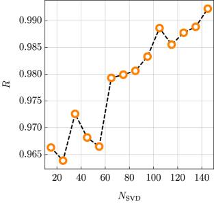
Figure 1: Values of the $R$ coefficient, see Eq. (42), as a function of the SVD subspace size for the HF molecule (internuclear distance $0.917\,$Å, cc-pVTZ basis set). The black dashed lines are linear functions connecting two neighboring data points.

The derivation of the SVD-CCSDT+ correction presented in Sec. 2.3 relies on the assumption that the SVD subspace is closed under the action of the Fock operator. When the SVD subspace is incomplete this constitutes an approximation whose quality has to be verified numerically. To quantify the accuracy of Eq. (13) we consider the action of the Fock operator on the sum of all SVD vectors, i.e. $\sum_{XYZ}F|XYZ\rangle$. For brevity, we introduce the symbol $\Psi_{\rm SVD}=\sum_{XYZ}|XYZ\rangle$. The function $F\Psi_{\rm SVD}$ is projected separately onto the SVD subspace and onto the full space of triple excitations. Finally, square norms of both projections are formed and the square root of their ratio is calculated. The resulting quantity measures the magnitude of the component of $F\Psi_{\rm SVD}$ that resides within the SVD subspace in relation to the total norm of the $F\Psi_{\rm SVD}$ function. Expressed mathematically, this reads

$$R=\sqrt{\frac{\langle\Psi_{\rm SVD}|F|XYZ\rangle\langle XYZ|F|\Psi_{\rm SVD}\rangle}{\langle\Psi_{\rm SVD}|F|_{ijk}^{abc}\rangle\langle_{ijk}^{abc}|F|\Psi_{\rm SVD}\rangle}}.$$ (42)

By construction, the coefficient $R$ takes values between $0$ and $1$. In a situation when Eq. (14) is satisfied exactly one strictly has $R=1$. Therefore, the deviation of the coefficient $R$ from the unity is a quantitative measure of the accuracy of the condition (14). However, it is important to point out that is not guaranteed that the coefficient $R$ vanishes monotonically as the SVD subspace size is increased.

As an illustrative example, we calculated the coefficient $R$ as a function of the SVD subspace size for the hydrogen fluoride (HF) molecule (internuclear distance $0.917\,$Å). For this system the maximum size of the SVD subspace equals to $195$. The results are presented in Fig. 1. The first important observation is that even for small SVD subspaces ($N_{\mathrm{SVD}}\approx 10$) the values of the coefficient $R$ are already larger than $0.95$. This further increases above $0.98$ when a larger number of SVD vectors are included ($N_{\mathrm{SVD}}\approx 50$). Therefore, for SVD subspaces large enough to be practically useful, the error resulting from Eq. (13) should not exceed a few percent. Considering other possible sources of error, this is acceptable from the point of view of the present work. In Supporting Information we present additional numerical results analogous to Fig. 1 for other molecules. The conclusions of these calculations are essentially the same as discussed above.

3.3 Accuracy of the SVD-CCSDT+ method:
total correlation energies

Before we present calculations of chemically-relevant quantities for larger molecular systems, it is advantageous to study errors of the SVD-CCSDT and SVD-CCSDT+ methods in reproduction of total correlation energies taking the exact CCSDT method as the reference. To this end we selected a set of $16$ small molecules comprising $2-5$ atoms. The list of the molecules together with their geometries in the Cartesian format are given in the Supporting Information. For each molecule we performed SVD-CCSDT and SVD-CCSDT+ calculations (cc-pVTZ basis set) with the size of the SVD subspace being linearly related to the total number of orbitals ($N_{\mathrm{MO}}$) in a given system, that is $N_{\mathrm{SVD}}=x\cdot N_{\mathrm{MO}}$. We consider several representative values of the $x$ parameter, namely $x=\frac{1}{6}$, $\frac{1}{3}$, $\frac{1}{2}$, $\frac{2}{3}$, $\frac{5}{6}$, $1$. To minimize the impact of the density-fitting approximation on the computed correlation energies, we employ a large cc-pV5Z-RI auxiliary basis set. With this setup the results are virtually free of the density-fitting error which does not exceed a few parts per million in all cases.

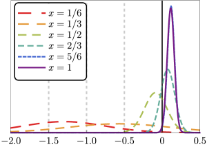
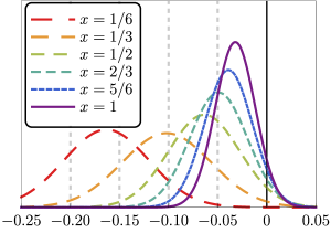
Figure 2: Distribution of relative errors (in percent) in the SVD-CCSDT (left panel) and SVD-CCSDT+ (right panel) correlation energies with respect to the exact CCSDT method (cc-pVTZ basis set). The parameter $x$ defines the size of the triple excitation subspace, $N_{\mathrm{SVD}}=x\cdot N_{\mathrm{MO}}$, where $N_{\mathrm{MO}}$ is the total number of orbitals in a given system. Notice the change of scale on the horizontal axis.

Further in this section we adopt the relative error in the correlation energy, defined as

$$\Delta_{i}=\frac{E_{\mathrm{method},i}-E_{\mathrm{CCSDT},i}}{E_{\mathrm{CCSDT},i}},$$ (43)

as the size-intensive measure of the quality of the results. In Eq. (20) the index $i$ enumerates the molecules in the test set and the symbol “method” refers to either SVD-CCSDT or SVD-CCSDT+. To perform a statistical analysis of the results we calculated the mean relative error and its standard deviation

$$\bar{\Delta}=\frac{1}{n}\sum_{i=1}^{n}\Delta_{i},$$ (44)

$$\Delta_{\mathrm{std}}^{2}=\frac{1}{n-1}\sum_{i=1}^{n}\left(\Delta_{i}-\bar{\Delta}\right)^{2},$$ (45)

where $n=16$ is the number of molecules in the test set. We found that the statistical distribution of the relative error is approximately normal for each value of the $x$ parameter. Therefore, to simplify the presentation the quantities $\bar{\Delta}$ and $\Delta_{\mathrm{std}}$ are represented graphically in Fig. 2 in terms of the Gaussian functions

$$\rho(\Delta)=\mathcal{N}e^{-\left(\Delta-\bar{\Delta}\right)^{2}/2\Delta_{\mathrm{std}}^{2}},$$ (46)

where $\mathcal{N}$ is a constant chosen such that $\rho(\Delta)$ is normalized to the unity. Raw values of the quantities $\bar{\Delta}$ and $\Delta_{\mathrm{std}}$ for all $x$ under consideration are given in the Supporting Information.

The results represented in Fig. 2 show that the SVD-CCSDT method has a tendency to underestimate the correlation energies for small $x$, but then it overshoots the exact results as $x$ is increased. For $x=1$ the mean error of the SVD-CCSDT method is slightly above 0.1% and, as demonstrated in Ref.  38, further increase of the parameter $x$ leads to a smooth, albeit slower, convergence towards the exact value. The behavior of the SVD-CCSDT+ is both qualitatively and quantitatively different. First, the overshooting tendency is absent and the convergence is smooth starting with the smallest $x$ considered here. Second, the magnitude of the error is reduced considerably; for example, for $x=1$ the SVD-CCSDT+ method achieves the mean relative error of about $-$0.03% which is by a factor of about four smaller than SVD-CCSDT. It is worth point out that for all molecules considered here, the SVD-CCSDT+ results approach their limit from above in a regular fashion. This opens up a possibility of extrapolation similar as in Refs.  115, 116, but a detailed analysis of this problem is beyond the scope of the present work.

3.4 Accuracy of the SVD-CCSDT+ method: relative energies

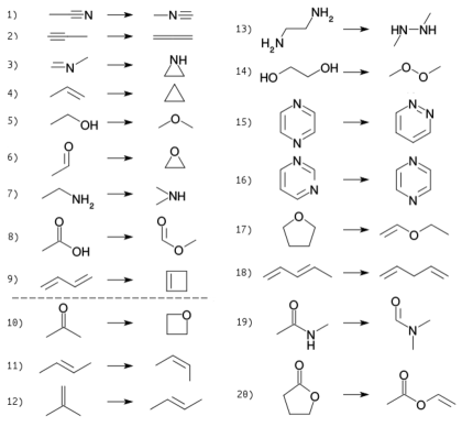
Figure 3: List of isomerization reactions considered in the present work. The horizontal dashed line separates two groups of reactions, see the discussion in Sec. 3.4.

Table 1: Isomerization energies (in kJ/mol) for systems presented in Fig. 3 calculated with the SVD-CCSDT and SVD-CCSDT+ methods as a function of the SVD subspace size ($N_{\mathrm{SVD}}$). For each reaction, the SVD-CCSDT results are given in the first row while the SVD-CCSDT+ results in the second row. The corresponding results obtained with the exact CCSDT method are given in the last column. The number of (active) occupied/virtual orbitals in each system is given in parentheses below the reaction numbers.

no.		$N_{\mathrm{SVD}}$							CCSDT
	$20$	$40$	$60$	$80$	$100$	$120$	$140$	$160$
1	105.50	102.21	101.11	101.47	101.02	101.05	101.10	100.95	100.79
(8/121)	100.70	100.46	100.66	100.69	100.78	100.75	100.72	100.72
2	8.69	7.03	6.99	6.49	5.33	5.55	5.37	5.18	4.43
(8/135)	4.55	4.31	4.34	4.47	4.58	4.53	4.52	4.52
3	49.65	46.03	46.61	46.57	45.90	46.06	45.88	45.92	45.99
(9/148)	45.95	45.80	45.78	45.81	45.86	45.88	45.88	45.89
4	35.31	32.72	33.64	32.85	32.29	32.47	32.40	32.30	32.13
(9/162)	32.20	32.00	31.96	31.95	31.98	31.98	32.04	32.05
5	49.86	49.76	50.00	50.00	49.66	49.19	49.00	49.00	48.80
(10/161)	48.88	48.87	48.85	48.84	48.79	48.77	48.78	48.77
6	—a	114.03	114.16	113.67	113.12	112.90	112.69	112.62	112.44
(9/134)	—a	112.48	112.45	112.38	112.40	112.38	112.38	112.37
7	34.15	34.52	34.41	34.27	31.15	33.98	33.86	33.89	33.67
(10/175)	33.74	33.73	33.76	33.68	33.68	33.66	33.66	33.65
8	69.77	70.79	70.20	70.33	69.73	69.68	69.44	69.36	69.12
(12/160)	69.29	69.24	69.22	69.19	69.17	69.16	69.15	69.14
9	52.44	50.32	49.67	50.52	49.63	48.88	48.80	48.82	48.85
(11/189)	48.93	48.85	48.80	48.70	48.65	48.60	48.67	48.69

^a SVD-CCSDT iterations did not converge.

In the previous we have considered the accuracy of the SVD-CCSDT+ method in reproduction of the total correlation energies. However, relative quantities are of prime importance in most practical situations. To analyze the accuracy and computational efficiency of the proposed method in the latter case we calculated isomerization energies for $20$ organic systems from the set previously considered by Grimme et al ¹¹⁷. This set covers a wide range of structural changes – from relatively simple cis-trans isomerizations to migrations of whole functional groups. Besides several reactions involving only hydrocarbons, we include examples that also involve heteroatoms (oxygen and nitrogen) to cover the most common bonding situations found in organic molecules. The range of isomerization energies is also broad, spanning from only a few kJ/mol to hundreds of kJ/mol. The list of isomerization reactions is given in Fig. 3. They are arranged roughly in the order of increasing system size. The largest molecule considered in this work (reaction 20) contains 46 electrons (34 correlated) with 264 functions in the atomic basis set and 666 functions in the density-fitting basis set. All reactions given in Fig. 3 are formulated such that the isomerization energies are positive.

The isomerization reactions given in Fig. 3 are divided into two groups. The first group (reactions 1–9) involve relatively small molecular systems for which full (uncompressed) CCSDT computations are available. This allows to ascertain the accuracy of the SVD-CCSDT+ method unambiguously. The second group (reactions 11–20) includes also larger species for which the exact CCSDT calculations are not practical with our computational resources. For each isomerization reaction from Fig. 3 we carried out SVD-CCSDT calculations followed by evaluation of the SVD-CCSDT+ correction. The size of the SVD subspace was varied from $N_{\mathrm{SVD}}=20$ up to $N_{\mathrm{SVD}}=160$ in steps of $20$. For the second group of reactions we additionally obtained results for $N_{\mathrm{SVD}}=180$ and $N_{\mathrm{SVD}}=200$ to fully converge the energy differences. The results for the first and second group of reactions are given in Tables 1 and 2, respectively.

We begin our analysis by considering the first group of reactions, see Table 1. Similarly as in the previous work, the SVD-CCSDT results converge rather quickly to the accuracy level of a fraction of 1 kJ/mol with increasing SVD subspace size. Beyond this point the convergence slows down (reactions 5 and 6) or even becomes mildly oscillatory (reactions 4 and 7). To reduce the error of the SVD-CCSDT method to the level of about 0.1 kJ/mol in all cases, a further increase of $N_{\mathrm{SVD}}$ would be needed. This is similar to the accuracy of the SVD-CCSDT method for the total correlation energies reported in Sec. 3.3 and in Ref.  38, albeit for the isomerization energies we do not observe the overshooting tendency.

By adding the SVD-CCSDT+ correction the results improve considerably. The accuracy of a fraction of 1 kJ/mol is achieved with significantly smaller SVD subspaces ($N_{\mathrm{SVD}}=40-60$). A further increase of $N_{\mathrm{SVD}}$ to $\approx N_{\mathrm{MO}}$ allows to stabilize the results to within 0.01–0.02 kJ/mol (or 0.02–0.03% on the relative basis) in most cases. Therefore, the overall behavior of the SVD-CCSDT+ method in calculation of the isomerization energies is similar as in the case of the total energies reported in Sec. 3.3. However, the improvement over the SVD-CCSDT is larger which suggests that the SVD-CCSDT+ method benefits from a more systematic error cancellation.

A puzzling feature of the SVD-CCSDT+ results is that despite the apparently tight convergence to within 0.01–0.02 kJ/mol for $N_{\mathrm{SVD}}\approx N_{\mathrm{MO}}$, the true errors with respect to the exact CCSDT are larger. On a relative basis, this phenomenon is most pronounced for reaction 2 where the SVD-CCSDT+ results for $N_{\mathrm{SVD}}=160$ are converged to within 0.01 kJ/mol, but the deviation from the exact CCSDT is about 0.09 kJ/mol. Some of this difference can clearly be attributed to the perturbative nature of the SVD-CCSDT+ method and additional simplifications described in Sec. 2.3. However, the density-fitting approximation of the two-electron integrals may also be suspected to bring a significant contribution to the observed deviation. In fact, density-fitting errors of a similar magnitude were observed in the DF-CCSD(T) method, see Ref.  16 for a detailed analysis. To study this issue we repeated the SVD-CCSDT+ calculations for reaction 2 within the same orbital basis set, but increased the size of the auxiliary basis set by one cardinal number. The isomerization energy obtained in this way for $N_{\mathrm{SVD}}=160$ turned out to be 4.47 kJ/mol, compared with 4.52 kJ/mol obtained previously. This reduced the deviation from the exact CCSDT result (4.43 kJ/mol) by a factor of two. Further increase of the size of the auxiliary basis leads to no appreciable improvement in the results. Therefore, we recommend to increase the size of the auxiliary basis set by one cardinal number in the SVD-CCSDT+ calculations if the accuracy of 0.1 kJ/mol or better is desired. Alternatively, other methods designed to reduce the density-fitting error can be adopted ^{118, 119} or the density-fitting approximation can be entirely replaced by the Cholesky decomposition ^{94, 95, 96, 97} where a stricter error control is possible.

Table 2: Isomerization energies (in kJ/mol) for systems presented in Fig. 3 calculated with the SVD-CCSDT and SVD-CCSDT+ methods as a function of the SVD subspace size ($N_{\mathrm{SVD}}$). For each reaction, the SVD-CCSDT results are given in the first row while the SVD-CCSDT+ results in the second row. The number of (active) occupied/virtual orbitals in each system is given in parentheses below the reaction numbers.

no.	$N_{\mathrm{SVD}}$
	$20$	$40$	$60$	$80$	$100$	$120$	$140$	$160$	$180$	$200$
10	133.22	133.27	132.53	132.18	132.42	131.54	131.46	131.23	131.27	131.02
(12/188)	130.80	130.65	130.75	130.65	130.63	130.54	130.53	130.53	130.54	130.53
11	4.97	5.06	4.63	4.78	4.67	4.71	4.79	4.67	4.73	4.68
(12/216)	4.57	4.69	4.66	4.61	4.65	4.63	4.64	4.64	4.65	4.65
12	3.90	4.45	4.90	4.19	4.66	4.67	4.57	4.63	4.59	4.55
(12/216)	4.59	4.66	4.66	4.67	4.67	4.66	4.64	4.66	4.65	4.65
13	118.61	117.90	117.66	117.68	117.63	117.08	116.95	116.61	116.45	116.46
(13/215)	116.44	116.28	116.25	116.20	116.17	116.10	116.11	116.10	116.10	116.09
14	273.71	270.06	271.01	270.74	269.29	268.74	268.46	268.27	268.13	268.08
(13/187)	268.00	267.62	267.62	267.45	267.42	267.37	267.34	267.32	267.31	267.30
15	77.34	76.29	76.00	76.46	75.56	76.76	75.52	75.70	75.53	75.55
(15/215)	75.66	75.57	75.59	75.55	75.57	75.51	75.50	75.50	75.48	75.48
16	19.89	18.37	20.51	19.74	20.88	19.94	20.15	19.81	20.02	19.87
(15/215)	18.99	19.37	19.41	19.49	19.44	19.47	19.46	19.45	19.46	19.46
17	49.24	49.70	50.08	49.95	50.63	50.82	51.91	52.49	52.56	52.71
(15/242)	52.70	52.84	52.90	52.98	53.02	53.03	53.01	53.02	53.01	53.02
18	27.75	24.90	25.20	25.54	25.60	25.72	25.88	26.08	26.10	26.22
(14/243)	26.98	26.79	26.78	26.85	26.82	26.80	26.82	26.82	26.83	26.83
19	39.52	40.35	40.14	39.54	39.69	39.48	39.59	39.24	39.02	39.01
(15/228)	38.60	38.70	38.61	38.63	38.60	38.59	38.57	38.54	38.53	38.53
20	58.98	59.41	59.21	59.03	59.45	60.32	61.12	61.44	61.73	61.98
(17/241)	62.43	62.42	62.56	62.67	62.73	62.75	62.76	62.77	62.75	62.76

Among the isomerizations considered in Table 1 the reaction 1 requires some additional attention. For this system an unexpectedly large discrepancy has been found between the CCSD(T) results published recently ¹¹⁷ and the available experimental data ^{120, 121, 122, 123}. While the CCSD(T) isomerization energy from Ref.  117 is 101.3 kJ/mol, the experimental result reads 89.1 kJ/mol. As argued in Ref.  117 this substantial difference of about 12 kJ/mol cannot be explained by effects such as the basis set incompleteness, core-valence correlation contributions, relativity or zero-point vibrational energy corrections. This led to the conclusion that the experimental uncertainty is the most likely source of the problem. However, it is worthwhile to analyze whether the post-CCSD(T) effects may explain the discrepancy. To this end we carried out additional CCSD(T) and SVD-CCSDT+ calculations using cc-pVQZ orbital basis set. We obtained $-0.77$ kJ/mol difference between CCSD(T) and SVD-CCSDT+ results for $N_{\mathrm{SVD}}=200$. This result is converged to within $0.01-0.02$ kJ/mol with respect to the size of the SVD subspace. Within the smaller cc-pVTZ basis set the analogous result reads $-0.56$ kJ/mol. To further minimize the finite basis set error we employed the two-point (cc-pVTZ/cc-pVQZ) Riemann extrapolation ¹²⁴ towards the complete basis set limit. This gives the final estimation of $-0.97$ kJ/mol for the difference between CCSD(T) and CCSDT isomerization energies of reaction 1. Clearly, this value is too small to explain the observed difference between theory and experiment, supporting the conclusions of Ref.  117. The example of reaction 1 also demonstrates the usefulness of the SVD-CCSDT+ method in computation of the “pure” post-CCSD(T) effects which are known to be difficult to reproduce accurately for polyatomic molecules¹²⁵.

Finally, let us consider the second group of isomerization reactions. The results obtained with SVD-CCSDT and SVD-CCSDT+ methods are given in Table 2. Since this group of reactions involves larger molecules, we additionally include results obtained for $N_{\mathrm{SVD}}=180$ and $N_{\mathrm{SVD}}=200$. In general, the picture drawn from the data presented in Table 2 is analogous as discussed above. In all cases, with $N_{\mathrm{SVD}}=160-200$ the SVD-CCSDT+ results are essentially converged to within 0.01–0.02 kJ/mol. Taking other sources of error into account one can estimate that the difference with respect to the exact CCSDT method is, on average, smaller than 0.1 kJ/mol in this regime. At the same time, if the accuracy level of a few tenths of kJ/mol is sufficient, reliable results can be obtained with small SVD subspaces, $N_{\mathrm{SVD}}=20-40$. This is a considerable advantage of the SVD-CCSDT+ method over SVD-CCSDT as the latter is not trustworthy in the small $N_{\mathrm{SVD}}$ regime.

Last but not least, let us discuss the timings of the SVD-CCSDT+ calculations. As an illustrative example let us consider the product of reaction 15 (236 orbital basis set functions, 606 auxiliary basis set functions, 30 correlated electrons). For this system $N_{\mathrm{SVD}}=120$ is sufficient to converge the SVD-CCSDT+ results to within a few hundreds of kJ/mol. As a reference point, CCSD calculations for this system take approximately 520 min (converged within 18 iterations). Determination of the SVD subspace takes about 567 min, in a reasonable agreement with rough estimations made in Supporting Information. The SVD-CCSDT calculations for $N_{\mathrm{SVD}}=120$ take 1943 min (22 iterations). Therefore, the total computational cost of the SVD-CCSDT method is about five times that of CCSD for this molecule. Finally, the evaluation of the SVD-CCSDT+ correction takes ca. 815 min; by comparison, computation of the standard (T) correction takes about 300 min. Despite this overhead is non-negligible, we believe that this is a reasonable price to pay for a sizable reduction of the error in the final results. All timings reported in this paragraph were obtained using a single core of AMD Opteron^TM 6174 processor without parallelization of the program execution and without exploitation of the point group symmetry.

4 Conclusions and future work

In this paper we have reported two novel developments in the field of the rank-reduced CCSDT theory. First, we have introduced a non-iterative energy correction, abbreviated as SVD-CCSDT+, added on top of the converged SVD-CCSDT result in order to approximately account for the triple excitations excluded from the parent SVD subspace. The working formula for the correction has been derived by extending the Lagrangian formalism of Eriksen et al. ⁷¹ with an additional assumption that the SVD subspace is closed under the action of the Fock operator. We have shown that in the limit of complete SVD subspace the value of the correction is rigorously equal to zero. In the opposite case of an empty SVD subspace the formula for the correction reduces to the well-known (T) method if sub-dominant terms that are at least quadratic in the cluster amplitudes are neglected.

The accuracy and computational efficiency of the proposed SVD-CCSDT+ correction has been assessed by studying a set of isomerization reactions involving small and medium-sized molecular systems. We have concluded that the non-iterative correction can fulfill two separate roles. If an accuracy level of a fraction of kJ/mol is sufficient, SVD-CCSDT+ correction significantly reduces the size of the SVD subspace that has to be employed in the iterative part of the calculations. Simultaneously, by adding the SVD-CCSDT+ correction the error due to the incompleteness of the SVD subspace can be reduced to levels considerably below 0.1 kJ/mol if the SVD subspace size is large enough. This levels of accuracy are usually impossible to achieve in practice solely with the SVD-CCSDT method. We have also presented representative timings of the SVD-CCSDT and SVD-CCSDT+ calculations, proving that the exact CCSDT results can be reproduced to within 0.1 kJ/mol with the computational cost only several times larger than required for the CCSD method. The SVD-CCSDT+ method retains black-box features of single-reference CC; the size of the SVD subspace remains the only additional parameter that has to be specified.

The second theoretical development introduced in this work is an algorithm for determination of the triples excitations subspace which is an alternative to the scheme given in Ref.  37. While the formalism proposed here is less general than the bidiagonalization strategy from Ref.  37, it scales rigorously as $N^{6}$, rather than $N^{7}$, with the system size. Therefore, despite a larger prefactor the proposed method is advantageous in applications to larger systems. Moreover, the new method comprises no iterative steps which eliminates accumulation of numerical noise and convergence problems one may encounter in iterative schemes.

As a final note, in the present work it has been demonstrated that the rank-reduced SVD-CCSDT+ method can reliably reproduce the exact CCSDT energetics with significantly decreased computational cost. The next important step is incorporation of quadruple excitation effects which become important at the 0.1 kJ/mol accuracy level. An economical way to take them into account is offered by non-iterative schemes such as CCSDT[Q] ^{126, 127, 128} or CCSDT(Q) ^{129, 130, 131}. In particular, the latter method was found to systematically improve the quality of the results ¹³², in comparison to both CCSD(T) and CCSDT, at a reasonable computational cost. Nowadays the CCSDT(Q) method is often regarded as the ”platinum standard“ of the electronic structure theory ¹³³, by analogy to the ”gold standard“ CCSD(T), and is a member of composite schemes routinely applied, e.g., in ab initio computational thermochemistry ^{134, 135, 136, 137, 138, 139, 140}. Unfortunately, incorporation of the (Q) correction in the present rank-reduced framework is not straightforward as its computational costs scale as $N^{9}$ with the system size if no approximations are introduced. This leads to a question whether by extending the rank-reduced CC formalism to the quadruply excited amplitudes one can reduce the scaling of the (Q) correction to a more manageable $N^{7}$ level, on par with the SVD-CCSDT+ theory. The answer to this question is affirmative and details of the procedure will be reported in a separate publication.

I would like to thank M. Mörchen, Dr. A. Tucholska and Prof. B. Jeziorski for fruitful discussions, and for reading and commenting on the manuscript. I am grateful to Prof. M. Reiher and all members of his group for their hospitality during my stay at Laboratorium für Physikalische Chemie, ETH Zürich. This work was supported by the Foundation for Polish Science (FNP) and by the Polish National Agency of Academic Exchange through the Bekker programme No. PPN/BEK/2019/1/00315/U/00001. Computations presented in this research were carried out with the support of the Interdisciplinary Center for Mathematical and Computational Modeling (ICM) at the University of Warsaw, grant number G86-1021.

The following file is available free of charge via the Internet at http://pubs.acs.org:

• plus-supp.pdf: derivation of the non-iterative method for determination of the SVD subspace described in Sec. 2.1, numerical verification of the scaling of the SVD-CCSDT+ method, additional numerical results confirming the conclusions of Sec. 3.2, Cartesian coordinates of molecular geometries used in Sec. 3.3, and statistical error measures for results presented in Sec. 3.3.

References

- Coester 1958 Coester, F. Bound states of a many-particle system. Nuc. Phys. 1958, 7, 421 – 424
- Coester and Kümmel 1960 Coester, F.; Kümmel, H. Short-range correlations in nuclear wave functions. Nuc. Phys. 1960, 17, 477 – 485
- C̆ížek 1966 C̆ížek, J. On the Correlation Problem in Atomic and Molecular Systems. Calculation of Wavefunction Components in Ursell-Type Expansion Using Quantum-Field Theoretical Methods. J. Chem. Phys. 1966, 45, 4256–4266
- C̆ížek 1966 C̆ížek, J. On the Use of the Cluster Expansion and the Technique of Diagrams in Calculations of Correlation Effects in Atoms and Molecules. Adv. Chem. Phys. 1966, 14, 35–89
- C̆ížek and Paldus 1971 C̆ížek, J.; Paldus, J. Correlation problems in atomic and molecular systems III. Rederivation of the coupled-pair many-electron theory using the traditional quantum chemical method. Int. J. Quantum Chem. 1971, 5, 359–379
- Paldus et al. 1972 Paldus, J.; C̆ížek, J.; Shavitt, I. Correlation Problems in Atomic and Molecular Systems. IV. Extended Coupled-Pair Many-Electron Theory and Its Application to the B Molecule. Phys. Rev. A 1972, 5, 50–67
- Crawford and Schaefer III 2000 Crawford, T. D.; Schaefer III, H. F. An Introduction to Coupled Cluster Theory for Computational Chemists. Rev. Comp. Chem. 2000, 14, 33–136
- Bartlett and Musiał 2007 Bartlett, R. J.; Musiał, M. Coupled-cluster theory in quantum chemistry. Rev. Mod. Phys. 2007, 79, 291–352
- Adamowicz and Bartlett 1987 Adamowicz, L.; Bartlett, R. J. Optimized virtual orbital space for high-level correlated calculations. J. Chem. Phys. 1987, 86, 6314–6324
- Adamowicz et al. 1988 Adamowicz, L.; Bartlett, R. J.; Sadlej, A. J. Optimized virtual orbital space for high-level correlated calculations. II. Electric properties. J. Chem. Phys. 1988, 88, 5749–5758
- Neogrády et al. 2005 Neogrády, P.; Pitoňák, M.; Urban, M. Optimized virtual orbitals for correlated calculations: an alternative approach. Mol. Phys. 2005, 103, 2141–2157
- Pitoňák et al. 2006 Pitoňák, M.; Holka, F.; Neogrády, P.; Urban, M. Optimized virtual orbitals for correlated calculations: Towards large scale CCSD(T) calculations of molecular dipole moments and polarizabilities. J. Mol. Struct. 2006, 768, 79 – 89
- Sosa et al. 1989 Sosa, C.; Geertsen, J.; Trucks, G. W.; Bartlett, R. J.; Franz, J. A. Selection of the reduced virtual space for correlated calculations. An application to the energy and dipole moment of H2O. Chem. Phys. Lett. 1989, 159, 148 – 154
- Taube and Bartlett 2006 Taube, A. G.; Bartlett, R. J. Frozen Natural Orbitals: Systematic Basis Set Truncation for Coupled-Cluster Theory. Collect. Czech. Chem. Commun. 2006, 70, 837–850
- Taube and Bartlett 2008 Taube, A. G.; Bartlett, R. J. Frozen natural orbital coupled-cluster theory: Forces and application to decomposition of nitroethane. J. Chem. Phys. 2008, 128, 164101
- DePrince and Sherrill 2013 DePrince, A. E.; Sherrill, C. D. Accuracy and Efficiency of Coupled-Cluster Theory Using Density Fitting/Cholesky Decomposition, Frozen Natural Orbitals, and a t1-Transformed Hamiltonian. J. Chem. Theory Comp. 2013, 9, 2687–2696
- Yang et al. 2011 Yang, J.; Kurashige, Y.; Manby, F. R.; Chan, G. K. L. Tensor factorizations of local second-order Møller-Plesset theory. J. Chem. Phys. 2011, 134, 044123
- Kurashige et al. 2012 Kurashige, Y.; Yang, J.; Chan, G. K.-L.; Manby, F. R. Optimization of orbital-specific virtuals in local Møller-Plesset perturbation theory. J. Chem. Phys. 2012, 136, 124106
- Yang et al. 2012 Yang, J.; Chan, G. K.-L.; Manby, F. R.; Schütz, M.; Werner, H.-J. The orbital-specific-virtual local coupled cluster singles and doubles method. J. Chem. Phys. 2012, 136, 144105
- Schütz et al. 2013 Schütz, M.; Yang, J.; Chan, G. K.-L.; Manby, F. R.; Werner, H.-J. The orbital-specific virtual local triples correction: OSV-L(T). J. Chem. Phys. 2013, 138, 054109
- Neese et al. 2009 Neese, F.; Wennmohs, F.; Hansen, A. Efficient and accurate local approximations to coupled-electron pair approaches: An attempt to revive the pair natural orbital method. J. Chem. Phys. 2009, 130, 114108
- Riplinger and Neese 2013 Riplinger, C.; Neese, F. An efficient and near linear scaling pair natural orbital based local coupled cluster method. J. Chem. Phys. 2013, 138, 034106
- Riplinger et al. 2013 Riplinger, C.; Sandhoefer, B.; Hansen, A.; Neese, F. Natural triple excitations in local coupled cluster calculations with pair natural orbitals. J. Chem. Phys. 2013, 139, 134101
- Liakos et al. 2015 Liakos, D. G.; Sparta, M.; Kesharwani, M. K.; Martin, J. M. L.; Neese, F. Exploring the Accuracy Limits of Local Pair Natural Orbital Coupled-Cluster Theory. J. Chem. Theory Comput. 2015, 11, 1525–1539
- Schwilk et al. 2017 Schwilk, M.; Ma, Q.; Köppl, C.; Werner, H.-J. Scalable Electron Correlation Methods. 3. Efficient and Accurate Parallel Local Coupled Cluster with Pair Natural Orbitals (PNO-LCCSD). J. Chem. Theory Comput. 2017, 13, 3650–3675
- Kolda and Bader 2009 Kolda, T. G.; Bader, B. W. Tensor Decompositions and Applications. SIAM Review 2009, 51, 455–500
- Scuseria et al. 2008 Scuseria, G. E.; Henderson, T. M.; Sorensen, D. C. The ground state correlation energy of the random phase approximation from a ring coupled cluster doubles approach. J. Chem. Phys. 2008, 129, 231101
- Bell et al. 2010 Bell, F.; Lambrecht, D.; Head-Gordon, M. Higher order singular value decomposition in quantum chemistry. Mol. Phys. 2010, 108, 2759–2773
- Kinoshita et al. 2003 Kinoshita, T.; Hino, O.; Bartlett, R. J. Singular value decomposition approach for the approximate coupled-cluster method. J. Chem. Phys. 2003, 119, 7756–7762
- Hino et al. 2004 Hino, O.; Kinoshita, T.; Bartlett, R. J. Singular value decomposition applied to the compression of T3 amplitude for the coupled cluster method. J. Chem. Phys. 2004, 121, 1206–1213
- Benedikt et al. 2011 Benedikt, U.; Auer, A. A.; Espig, M.; Hackbusch, W. Tensor decomposition in post-Hartree-Fock methods. I. Two-electron integrals and MP2. J. Chem. Phys. 2011, 134, 054118
- Benedikt et al. 2013 Benedikt, U.; Böhm, K.-H.; Auer, A. A. Tensor decomposition in post-Hartree-Fock methods. II. CCD implementation. J. Chem. Phys. 2013, 139, 224101
- Schutski et al. 2017 Schutski, R.; Zhao, J.; Henderson, T. M.; Scuseria, G. E. Tensor-structured coupled cluster theory. J. Chem. Phys. 2017, 147, 184113
- Mayhall 2017 Mayhall, N. J. Using Higher-Order Singular Value Decomposition To Define Weakly Coupled and Strongly Correlated Clusters: The n-Body Tucker Approximation. J. Chem. Theory Comput. 2017, 13, 4818–4828
- Parrish et al. 2019 Parrish, R. M.; Zhao, Y.; Hohenstein, E. G.; Martínez, T. J. Rank reduced coupled cluster theory. I. Ground state energies and wavefunctions. J. Chem. Phys. 2019, 150, 164118
- Hohenstein et al. 2019 Hohenstein, E. G.; Zhao, Y.; Parrish, R. M.; Martínez, T. J. Rank reduced coupled cluster theory. II. Equation-of-motion coupled-cluster singles and doubles. J. Chem. Phys. 2019, 151, 164121
- Lesiuk 2019 Lesiuk, M. Efficient singular-value decomposition of the coupled-cluster triple excitation amplitudes. J. Comp. Chem. 2019, 40, 1319–1332
- Lesiuk 2020 Lesiuk, M. Implementation of the Coupled-Cluster Method with Single, Double, and Triple Excitations using Tensor Decompositions. J. Chem. Theory Comput. 2020, 16, 453–467
- Hohenstein et al. 2012 Hohenstein, E. G.; Parrish, R. M.; Martínez, T. J. Tensor hypercontraction density fitting. I. Quartic scaling second- and third-order Møller-Plesset perturbation theory. J. Chem. Phys. 2012, 137, 044103
- Parrish et al. 2012 Parrish, R. M.; Hohenstein, E. G.; Martínez, T. J.; Sherrill, C. D. Tensor hypercontraction. II. Least-squares renormalization. J. Chem. Phys. 2012, 137, 224106
- Parrish et al. 2013 Parrish, R. M.; Hohenstein, E. G.; Martínez, T. J.; Sherrill, C. D. Discrete variable representation in electronic structure theory: Quadrature grids for least-squares tensor hypercontraction. J. Chem. Phys. 2013, 138, 194107
- Kokkila Schumacher et al. 2015 Kokkila Schumacher, S. I. L.; Hohenstein, E. G.; Parrish, R. M.; Wang, L.-P.; Martínez, T. J. Tensor Hypercontraction Second-Order Møller-Plesset Perturbation Theory: Grid Optimization and Reaction Energies. J. Chem. Theory Comput. 2015, 11, 3042–3052
- Lu and Ying 2015 Lu, J.; Ying, L. Compression of the electron repulsion integral tensor in tensor hypercontraction format with cubic scaling cost. J. Comp. Chem. 2015, 302, 329 – 335
- Lee et al. 2020 Lee, J.; Lin, L.; Head-Gordon, M. Systematically Improvable Tensor Hypercontraction: Interpolative Separable Density-Fitting for Molecules Applied to Exact Exchange, Second- and Third-Order Møller-Plesset Perturbation Theory. J. Chem. Theory Comput. 2020, 16, 243–263
- Matthews 2020 Matthews, D. A. Improved Grid Optimization and Fitting in Least Squares Tensor Hypercontraction. J. Chem. Theory Comput. 2020, 16, 1382–1385
- Hohenstein et al. 2012 Hohenstein, E. G.; Parrish, R. M.; Sherrill, C. D.; Martínez, T. J. Communication: Tensor hypercontraction. III. Least-squares tensor hypercontraction for the determination of correlated wavefunctions. J. Chem. Phys. 2012, 137, 221101
- Hohenstein et al. 2013 Hohenstein, E. G.; Kokkila, S. I. L.; Parrish, R. M.; Martínez, T. J. Quartic scaling second-order approximate coupled cluster singles and doubles via tensor hypercontraction: THC-CC2. J. Chem. Phys. 2013, 138, 124111
- Hohenstein et al. 2013 Hohenstein, E. G.; Kokkila, S. I. L.; Parrish, R. M.; Martínez, T. J. Tensor Hypercontraction Equation-of-Motion Second-Order Approximate Coupled Cluster: Electronic Excitation Energies in O() Time. J. Phys. Chem. B 2013, 117, 12972–12978
- Shenvi et al. 2013 Shenvi, N.; van Aggelen, H.; Yang, Y.; Yang, W.; Schwerdtfeger, C.; Mazziotti, D. The tensor hypercontracted parametric reduced density matrix algorithm: Coupled-cluster accuracy with O() scaling. J. Chem. Phys. 2013, 139, 054110
- Shenvi et al. 2014 Shenvi, N.; van Aggelen, H.; Yang, Y.; Yang, W. Tensor hypercontracted ppRPA: Reducing the cost of the particle-particle random phase approximation from O() to O(). J. Chem. Phys. 2014, 141, 024119
- Parrish et al. 2014 Parrish, R. M.; Sherrill, C. D.; Hohenstein, E. G.; Kokkila, S. I. L.; Martínez, T. J. Communication: Acceleration of coupled cluster singles and doubles via orbital-weighted least-squares tensor hypercontraction. J. Chem. Phys. 2014, 140, 181102
- Lu and Thicke 2017 Lu, J.; Thicke, K. Cubic scaling algorithms for RPA correlation using interpolative separable density fitting. J. Comp. Phys. 2017, 351, 187 – 202
- Song and Martínez 2016 Song, C.; Martínez, T. J. Atomic orbital-based SOS-MP2 with tensor hypercontraction. I. GPU-based tensor construction and exploiting sparsity. J. Chem. Phys. 2016, 144, 174111
- Song and Martínez 2017 Song, C.; Martínez, T. J. Atomic orbital-based SOS-MP2 with tensor hypercontraction. II. Local tensor hypercontraction. J. Chem. Phys. 2017, 146, 034104
- Song and Martínez 2018 Song, C.; Martínez, T. J. Reduced scaling CASPT2 using supporting subspaces and tensor hyper-contraction. J. Chem. Phys. 2018, 149, 044108
- Tucker 1966 Tucker, L. R. Some mathematical notes on three-mode factor analysis. Psychometrika 1966, 31, 279–311
- De Lathauwer et al. 2000 De Lathauwer, L.; De Moor, B.; Vandewalle, J. A Multilinear Singular Value Decomposition. SIAM J. Matrix Anal. Appl. 2000, 21, 1253–1278
- Noga and Bartlett 1987 Noga, J.; Bartlett, R. J. The full CCSDT model for molecular electronic structure. J. Chem. Phys. 1987, 86, 7041–7050
- Scuseria and Schaefer 1988 Scuseria, G. E.; Schaefer, H. F. A new implementation of the full CCSDT model for molecular electronic structure. Chem. Phys. Lett. 1988, 152, 382 – 386
- Møller and Plesset 1934 Møller, C.; Plesset, M. S. Note on an Approximation Treatment for Many-Electron Systems. Phys. Rev. 1934, 46, 618–622
- Raghavachari et al. 1989 Raghavachari, K.; Trucks, G. W.; Pople, J. A.; Head-Gordon, M. A fifth-order perturbation comparison of electron correlation theories. Chem. Phys. Lett. 1989, 157, 479 – 483
- Noga et al. 1987 Noga, J.; Bartlett, R. J.; Urban, M. Towards a full CCSDT model for electron correlation. CCSDT-n models. Chem. Phys. Lett. 1987, 134, 126 – 132
- Stanton 1997 Stanton, J. F. Why CCSD(T) works: a different perspective. Chem. Phys. Lett. 1997, 281, 130 – 134
- Stanton and Bartlett 1993 Stanton, J. F.; Bartlett, R. J. The equation of motion coupled-cluster method. A systematic biorthogonal approach to molecular excitation energies, transition probabilities, and excited state properties. J. Chem. Phys. 1993, 98, 7029–7039
- Gwaltney and Head-Gordon 2000 Gwaltney, S. R.; Head-Gordon, M. A second-order correction to singles and doubles coupled-cluster methods based on a perturbative expansion of a similarity-transformed Hamiltonian. Chem. Phys. Lett. 2000, 323, 21 – 28
- Gwaltney and Head-Gordon 2001 Gwaltney, S. R.; Head-Gordon, M. A second-order perturbative correction to the coupled-cluster singles and doubles method: CCSD(2). J. Chem. Phys. 2001, 115, 2014–2021
- Hirata et al. 2001 Hirata, S.; Nooijen, M.; Grabowski, I.; Bartlett, R. J. Perturbative corrections to coupled-cluster and equation-of-motion coupled-cluster energies: A determinantal analysis. J. Chem. Phys. 2001, 114, 3919–3928
- Hirata et al. 2004 Hirata, S.; Fan, P.-D.; Auer, A. A.; Nooijen, M.; Piecuch, P. Combined coupled-cluster and many-body perturbation theories. J. Chem. Phys. 2004, 121, 12197–12207
- Shiozaki et al. 2007 Shiozaki, T.; Hirao, K.; Hirata, S. Second- and third-order triples and quadruples corrections to coupled-cluster singles and doubles in the ground and excited states. J. Chem. Phys. 2007, 126, 244106
- Eriksen et al. 2014 Eriksen, J. J.; Jørgensen, P.; Olsen, J.; Gauss, J. Equation-of-motion coupled cluster perturbation theory revisited. J. Chem. Phys. 2014, 140, 174114
- Eriksen et al. 2014 Eriksen, J.; Kristensen, K.; Kjærgaard, T.; Jørgensen, P.; Gauss, J. A Lagrangian framework for deriving triples and quadruples corrections to the CCSD energy. J. Chem. Phys. 2014, 140, 064108
- Kristensen et al. 2016 Kristensen, K.; Eriksen, J. J.; Matthews, D. A.; Olsen, J.; Jørgensen, P. A view on coupled cluster perturbation theory using a bivariational Lagrangian formulation. J. Chem. Phys. 2016, 144, 064103
- Pawłowski et al. 2019 Pawłowski, F.; Olsen, J.; Jørgensen, P. Cluster perturbation theory. I. Theoretical foundation for a coupled cluster target state and ground-state energies. J. Chem. Phys. 2019, 150, 134108
- Pawłowski et al. 2019 Pawłowski, F.; Olsen, J.; Jørgensen, P. Cluster perturbation theory. II. Excitation energies for a coupled cluster target state. J. Chem. Phys. 2019, 150, 134109
- Baudin et al. 2019 Baudin, P.; Pawłowski, F.; Bykov, D.; Liakh, D.; Kristensen, K.; Olsen, J.; Jørgensen, P. Cluster perturbation theory. III. Perturbation series for coupled cluster singles and doubles excitation energies. J. Chem. Phys. 2019, 150, 134110
- Pawłowski et al. 2019 Pawłowski, F.; Olsen, J.; Jørgensen, P. Cluster perturbation theory. IV. Convergence of cluster perturbation series for energies and molecular properties. J. Chem. Phys. 2019, 150, 134111
- Pawłowski et al. 2019 Pawłowski, F.; Olsen, J.; Jørgensen, P. Cluster perturbation theory. V. Theoretical foundation for cluster linear target states. J. Chem. Phys. 2019, 150, 134112
- Kowalski and Piecuch 2000 Kowalski, K.; Piecuch, P. The method of moments of coupled-cluster equations and the renormalized CCSD[T], CCSD(T), CCSD(TQ), and CCSDT(Q) approaches. J. Chem. Phys. 2000, 113, 18–35
- Piecuch et al. 2002 Piecuch, P.; Kowalski, K.; Pimienta, I. S. O.; Mcguire, M. J. Recent advances in electronic structure theory: Method of moments of coupled-cluster equations and renormalized coupled-cluster approaches. Int. Rev. Phys. Chem. 2002, 21, 527–655
- Piecuch et al. 2004 Piecuch, P.; Kowalski, K.; Pimienta, I. S. O.; Fan, P.-D.; Lodriguito, M.; McGuire, M. J.; Kucharski, S. A.; Kuś, T.; Musiał, M. Method of moments of coupled-cluster equations: a new formalism for designing accurate electronic structure methods for ground and excited states. Theor. Chem. Acc. 2004, 112, 349–393
- Piecuch and Włoch 2005 Piecuch, P.; Włoch, M. Renormalized coupled-cluster methods exploiting left eigenstates of the similarity-transformed Hamiltonian. J. Chem. Phys. 2005, 123, 224105
- Shen and Piecuch 2012 Shen, J.; Piecuch, P. Biorthogonal moment expansions in coupled-cluster theory: Review of key concepts and merging the renormalized and active-space coupled-cluster methods. Chem. Phys. 2012, 401, 180–202
- Shen and Piecuch 2012 Shen, J.; Piecuch, P. Combining active-space coupled-cluster methods with moment energy corrections via the CC(P;Q) methodology, with benchmark calculations for biradical transition states. J. Chem. Phys. 2012, 136, 144104
- Shen and Piecuch 2012 Shen, J.; Piecuch, P. Merging Active-Space and Renormalized Coupled-Cluster Methods via the CC(P;Q) Formalism, with Benchmark Calculations for Singlet-Triplet Gaps in Biradical Systems. J. Chem. Theory Comput. 2012, 8, 4968–4988
- Paldus and Jeziorski 1988 Paldus, J.; Jeziorski, B. Clifford algebra and unitary group formulations of the many-electron problem. Theor. Chem. Acc. 1988, 73, 81–103
- Whitten 1973 Whitten, J. L. Coulombic potential energy integrals and approximations. J. Chem. Phys. 1973, 58, 4496–4501
- Baerends et al. 1973 Baerends, E.; Ellis, D.; Ros, P. Self-consistent molecular Hartree-Fock-Slater calculations I. The computational procedure. Chem. Phys. 1973, 2, 41 – 51
- Dunlap et al. 1979 Dunlap, B. I.; Connolly, J. W. D.; Sabin, J. R. On some approximations in applications of X theory. J. Chem. Phys. 1979, 71, 3396–3402
- Van Alsenoy 1988 Van Alsenoy, C. Ab initio calculations on large molecules: The multiplicative integral approximation. J. Comp. Chem. 1988, 9, 620–626
- Vahtras et al. 1993 Vahtras, O.; Almlöf, J.; Feyereisen, M. Integral approximations for LCAO-SCF calculations. Chem. Phys. Lett. 1993, 213, 514 – 518
- Katouda and Nagase 2009 Katouda, M.; Nagase, S. Efficient parallel algorithm of second-order Møller-Plesset perturbation theory with resolution-of-identity approximation (RI-MP2). Int. J. Quantum Chem. 2009, 109, 2121–2130
- Wirz et al. 2017 Wirz, L. N.; Reine, S. S.; Pedersen, T. B. On Resolution-of-the-Identity Electron Repulsion Integral Approximations and Variational Stability. J. Chem. Theory Comp. 2017, 13, 4897–4906
- Koch et al. 1994 Koch, H.; Christiansen, O.; Kobayashi, R.; Jørgensen, P.; Helgaker, T. A direct atomic orbital driven implementation of the coupled cluster singles and doubles (CCSD) model. Chem. Phys. Lett. 1994, 228, 233 – 238
- Beebe and Linderberg 1997 Beebe, N. H. F.; Linderberg, J. Simplifications in the generation and transformation of two-electron integrals in molecular calculations. Int. J. Quantum Chem. 1997, 12, 683–705
- Koch et al. 2003 Koch, H.; Sánchez de Merás, A.; Pedersen, T. B. Reduced scaling in electronic structure calculations using Cholesky decompositions. J. Chem. Phys. 2003, 118, 9481–9484
- Pedersen et al. 2004 Pedersen, T. B.; Sánchez de Merás, A. M. J.; Koch, H. Polarizability and optical rotation calculated from the approximate coupled cluster singles and doubles CC2 linear response theory using Cholesky decompositions. J. Chem. Phys. 2004, 120, 8887–8897
- Folkestad et al. 2019 Folkestad, S. D.; Kjønstad, E. F.; Koch, H. An efficient algorithm for Cholesky decomposition of electron repulsion integrals. J. Chem. Phys. 2019, 150, 194112
- Fitzgerald et al. 1986 Fitzgerald, G.; Harrison, R. J.; Bartlett, R. J. Analytic energy gradients for general coupled-cluster methods and fourth-order many-body perturbation theory. J. Chem. Phys. 1986, 85, 5143–5150
- Salter et al. 1989 Salter, E. A.; Trucks, G. W.; Bartlett, R. J. Analytic energy derivatives in many-body methods. I. First derivatives. J. Chem. Phys. 1989, 90, 1752–1766
- Jørgensen and Helgaker 1988 Jørgensen, P.; Helgaker, T. Møller-Plesset energy derivatives. J. Chem. Phys. 1988, 89, 1560–1570
- Helgaker et al. 1989 Helgaker, T.; Jørgensen, P.; Handy, N. C. A numerically stable procedure for calculating Møller-Plesset energy derivatives, derived using the theory of Lagrangians. Theor. Chem. Acc. 1989, 76, 227–245
- Koch et al. 1990 Koch, H.; Jensen, H. J. A.; Jørgensen, P.; Helgaker, T.; Scuseria, G. E.; Schaefer, H. F. Coupled cluster energy derivatives. Analytic Hessian for the closed-shell coupled cluster singles and doubles wave function: Theory and applications. J. Chem. Phys. 1990, 92, 4924–4940
- Koch et al. 1997 Koch, H.; Christiansen, O.; Jørgensen, P.; Sanchez de Merás, A. M.; Helgaker, T. The CC3 model: An iterative coupled cluster approach including connected triples. J. Chem. Phys. 1997, 106, 1808–1818
- Crawford and Stanton 1998 Crawford, T. D.; Stanton, J. F. Investigation of an asymmetric triple-excitation correction for coupled-cluster energies. Int. J. Quantum Chem. 1998, 70, 601–611
- Kucharski and Bartlett 1998 Kucharski, S. A.; Bartlett, R. J. Noniterative energy corrections through fifth-order to the coupled cluster singles and doubles method. J. Chem. Phys. 1998, 108, 5243–5254
- Lee et al. 1990 Lee, T. J.; Rendell, A. P.; Taylor, P. R. Comparison of the quadratic configuration interaction and coupled-cluster approaches to electron correlation including the effect of triple excitations. J. Phys. Chem. 1990, 94, 5463–5468
- Rendell et al. 1991 Rendell, A. P.; Lee, T. J.; Komornicki, A. A parallel vectorized implementation of triple excitations in CCSD(T): application to the binding energies of the AlH3, AlH2F, AlHF2 and AlF3 dimers. Chem. Phys. Lett. 1991, 178, 462 – 470
- Janowski and Pulay 2008 Janowski, T.; Pulay, P. Efficient Parallel Implementation of the CCSD External Exchange Operator and the Perturbative Triples (T) Energy Calculation. J. Chem. Theory Comput. 2008, 4, 1585–1592
- Dunning 1989 Dunning, T. H. Gaussian basis sets for use in correlated molecular calculations. I. The atoms boron through neon and hydrogen. J. Chem. Phys. 1989, 90, 1007–1023
- Weigend et al. 1998 Weigend, F.; Häser, M.; Patzelt, H.; Ahlrichs, R. RI-MP2: optimized auxiliary basis sets and demonstration of efficiency. Chem. Phys. Lett. 1998, 294, 143 – 152
- Weigend 2002 Weigend, F. A fully direct RI-HF algorithm: Implementation, optimised auxiliary basis sets, demonstration of accuracy and efficiency. Phys. Chem. Chem. Phys. 2002, 4, 4285–4291
- Schmidt et al. 1993 Schmidt, M. W.; Baldridge, K. K.; Boatz, J. A.; Elbert, S. T.; Gordon, M. S.; Jensen, J. H.; Koseki, S.; Matsunaga, N.; Nguyen, K. A.; Su, S.; Windus, T. L.; Dupuis, M.; Montgomery, J. A. General atomic and molecular electronic structure system. J. Comp. Chem. 1993, 14, 1347–1363
- 113 Stanton, J. F.; Gauss, J.; Cheng, L.; Harding, M. E.; Matthews, D. A.; Szalay, P. G. CFOUR, Coupled-Cluster techniques for Computational Chemistry, a quantum-chemical program package. With contributions from A.A. Auer, R.J. Bartlett, U. Benedikt, C. Berger, D.E. Bernholdt, S. Blaschke, Y. J. Bomble, S. Burger, O. Christiansen, D. Datta, F. Engel, R. Faber, J. Greiner, M. Heckert, O. Heun, M. Hilgenberg, C. Huber, T.-C. Jagau, D. Jonsson, J. Jusélius, T. Kirsch, K. Klein, G.M. KopperW.J. Lauderdale, F. Lipparini, T. Metzroth, L.A. Mück, D.P. O’Neill, T. Nottoli, D.R. Price, E. Prochnow, C. Puzzarini, K. Ruud, F. Schiffmann, W. Schwalbach, C. Simmons, S. Stopkowicz, A. Tajti, J. Vázquez, F. Wang, J.D. Watts and the integral packages MOLECULE (J. Almlöf and P.R. Taylor), PROPS (P.R. Taylor), ABACUS (T. Helgaker, H.J. Aa. Jensen, P. Jørgensen, and J. Olsen), and ECP routines by A. V. Mitin and C. van Wüllen. For the current version, see http://www.cfour.de.
- Matthews et al. 2020 Matthews, D. A.; Cheng, L.; Harding, M. E.; Lipparini, F.; Stopkowicz, S.; Jagau, T.-C.; Szalay, P. G.; Gauss, J.; Stanton, J. F. Coupled-cluster techniques for computational chemistry: The CFOUR program package. J. Chem. Phys. 2020, 152, 214108
- Landau et al. 2010 Landau, A.; Khistyaev, K.; Dolgikh, S.; Krylov, A. I. Frozen natural orbitals for ionized states within equation-of-motion coupled-cluster formalism. J. Chem. Phys. 2010, 132, 014109
- Segarra-Martí et al. 2018 Segarra-Martí, J.; Garavelli, M.; Aquilante, F. Converging many-body correlation energies by means of sequence extrapolation. J. Chem. Phys. 2018, 148, 034107
- Grimme et al. 2007 Grimme, S.; Steinmetz, M.; Korth, M. How to Compute Isomerization Energies of Organic Molecules with Quantum Chemical Methods. J. Org. Chem. 2007, 72, 2118–2126
- Schurkus et al. 2017 Schurkus, H. F.; Luenser, A.; Ochsenfeld, C. Communication: Almost error-free resolution-of-the-identity correlation methods by null space removal of the particle-hole interactions. J. Chem. Phys. 2017, 146, 211106
- Lesiuk 2020 Lesiuk, M. A straightforward a posteriori method for reduction of density-fitting error in coupled-cluster calculations. J. Chem. Phys. 2020, 152, 044104
- Baghal-Vayjooee et al. 1977 Baghal-Vayjooee, M. H.; Collister, J. L.; Pritchard, H. O. The enthalpy of isomerisation of methyl isocyanide. Can. J. Chem. 1977, 55, 2634–2636
- An and Månsson 1983 An, X.-W.; Månsson, M. Enthalpies of combustion and formation of acetonitrile. J. Chem. Thermodyn. 1983, 15, 287 – 293
- Pedley et al. 1986 Pedley, J. B.; Naylor, R. D.; Kirby, S. B. Thermochemical data of organic compounds; Springer Netherlands, 1986
- 123 Linstrom, P., Mallard, W., Eds. NIST Chemistry WebBook, NIST Standard Reference Database Number 69; National Institute of Standards and Technology
- Lesiuk and Jeziorski 2019 Lesiuk, M.; Jeziorski, B. Complete Basis Set Extrapolation of Electronic Correlation Energies Using the Riemann Zeta Function. J. Chem. Theory Comput. 2019, 15, 5398–5403
- Smith et al. 2014 Smith, D. G. A.; Jankowski, P.; Slawik, M.; Witek, H. A.; Patkowski, K. Basis Set Convergence of the Post-CCSD(T) Contribution to Noncovalent Interaction Energies. J. Chem. Theory Comput. 2014, 10, 3140–3150
- Kucharski and Bartlett 1989 Kucharski, S. A.; Bartlett, R. J. Coupled-cluster methods that include connected quadruple excitations, T4: CCSDTQ-1 and Q(CCSDT). Chem. Phys. Lett. 1989, 158, 550 – 555
- Kucharski and Bartlett 1998 Kucharski, S. A.; Bartlett, R. J. An efficient way to include connected quadruple contributions into the coupled cluster method. J. Chem. Phys. 1998, 108, 9221–9226
- Kucharski et al. 2001 Kucharski, S. A.; Kolaski, M.; Bartlett, R. J. Toward the limits of predictive electronic structure theory: Connected quadruple excitations for large basis set calculations. J. Chem. Phys. 2001, 114, 692–700
- Bomble et al. 2005 Bomble, Y. J.; Stanton, J. F.; Kállay, M.; Gauss, J. Coupled-cluster methods including noniterative corrections for quadruple excitations. J. Chem. Phys. 2005, 123, 054101
- Kállay and Gauss 2005 Kállay, M.; Gauss, J. Approximate treatment of higher excitations in coupled-cluster theory. J. Chem. Phys. 2005, 123, 214105
- Kállay and Gauss 2008 Kállay, M.; Gauss, J. Approximate treatment of higher excitations in coupled-cluster theory. II. Extension to general single-determinant reference functions and improved approaches for the canonical Hartree-Fock case. J. Chem. Phys. 2008, 129, 144101
- Eriksen et al. 2015 Eriksen, J. J.; Matthews, D. A.; Jørgensen, P.; Gauss, J. Communication: The performance of non-iterative coupled cluster quadruples models. J. Chem. Phys. 2015, 143, 041101
- Kodrycka and Patkowski 2019 Kodrycka, M.; Patkowski, K. Platinum, gold, and silver standards of intermolecular interaction energy calculations. J. Chem. Phys. 2019, 151, 070901
- Martin and de Oliveira 1999 Martin, J. M. L.; de Oliveira, G. Towards standard methods for benchmark quality ab initio thermochemistry – W1 and W2 theory. J. Chem. Phys. 1999, 111, 1843–1856
- Boese et al. 2004 Boese, A. D.; Oren, M.; Atasoylu, O.; Martin, J. M. L.; Kállay, M.; Gauss, J. W3 theory: Robust computational thermochemistry in the kJ/mol accuracy range. J. Chem. Phys. 2004, 120, 4129–4141
- Karton et al. 2006 Karton, A.; Rabinovich, E.; Martin, J. M. L.; Ruscic, B. W4 theory for computational thermochemistry: In pursuit of confident sub-kJ/mol predictions. J. Chem. Phys. 2006, 125, 144108
- Tajti et al. 2004 Tajti, A.; Szalay, P. G.; Császár, A. G.; Kállay, M.; Gauss, J.; Valeev, E. F.; Flowers, B. A.; Vázquez, J.; Stanton, J. F. HEAT: High accuracy extrapolated ab initio thermochemistry. J. Chem. Phys. 2004, 121, 11599–11613
- Bomble et al. 2006 Bomble, Y. J.; Vázquez, J.; Kállay, M.; Michauk, C.; Szalay, P. G.; Császár, A. G.; Gauss, J.; Stanton, J. F. High-accuracy extrapolated ab initio thermochemistry. II. Minor improvements to the protocol and a vital simplification. J. Chem. Phys. 2006, 125, 064108
- Harding et al. 2008 Harding, M. E.; Vázquez, J.; Ruscic, B.; Wilson, A. K.; Gauss, J.; Stanton, J. F. High-accuracy extrapolated ab initio thermochemistry. III. Additional improvements and overview. J. Chem. Phys. 2008, 128, 114111
- Feller et al. 2008 Feller, D.; Peterson, K. A.; Dixon, D. A. A survey of factors contributing to accurate theoretical predictions of atomization energies and molecular structures. J. Chem. Phys. 2008, 129, 204105