Measuring Fairness
Under Unawareness of Sensitive Attributes:
A Quantification-Based Approach

Abstract

Algorithms and models are increasingly deployed to inform decisions about people, inevitably affecting their lives. As a consequence, those in charge of developing these models must carefully evaluate their impact on different groups of people and favour group fairness, that is, ensure that groups determined by sensitive demographic attributes, such as race or sex, are not treated unjustly. To achieve this goal, the availability (awareness) of these demographic attributes to those evaluating the impact of these models is fundamental. Unfortunately, collecting and storing these attributes is often in conflict with industry practices and legislation on data minimisation and privacy. For this reason, it can be hard to measure the group fairness of trained models, even from within the companies developing them. In this work, we tackle the problem of measuring group fairness under unawareness of sensitive attributes, by using techniques from quantification, a supervised learning task concerned with directly providing group-level prevalence estimates (rather than individual-level class labels). We show that quantification approaches are particularly suited to tackle the fairness-under-unawareness problem, as they are robust to inevitable distribution shifts while at the same time decoupling the (desirable) objective of measuring group fairness from the (undesirable) side effect of allowing the inference of sensitive attributes of individuals. More in detail, we show that fairness under unawareness can be cast as a quantification problem and solved with proven methods from the quantification literature. We show that these methods outperform previous approaches to measure demographic parity in five experimental protocols, corresponding to important challenges that complicate the estimation of classifier fairness under unawareness.

1 Introduction

The widespread adoption of algorithmic decision-making in high-stakes domains has determined an increased attention to the underlying algorithms and their impact on people, with attention to sensitive (or “protected”) groups. Typically, sensitive groups are subpopulations determined by salient social and demographic factors, such as race or sex. The unfair treatment of such groups is not only unethical, but also ruled out by anti-discrimination laws, and is thus studied by a growing community of algorithmic fairness researchers. Important works in this area have addressed the unfair treatment of subpopulations that may arise in the judicial system (Angwin et al., 2016; Larson et al., 2016; Berk et al., 2021), healthcare (Obermeyer et al., 2019; Gervasi et al., 2022; Ricci Lara et al., 2022), search engines (Geyik et al., 2019; Fabris et al., 2020; Ekstrand et al., 2022), insurance (Angwin et al., 2017; Donahue and Barocas, 2021; Fabris et al., 2021), and computer vision (Buolamwini and Gebru, 2018; Raji and Buolamwini, 2019; Goyal et al., 2022), just to name a few domains that may be affected. One common trait of these research works is their attention to a careful definition (and subsequent measurement) of what it means for a model to be fair to the subgroups involved (group fairness), which is typically viewed in terms of differences, across the salient subpopulations, in quantities of interest such as accuracy, recall, or acceptance rate. According to popular definitions of fairness, sizeable such differences (e.g., between women and men) correspond to low fairness on the part of the algorithm (Dwork et al., 2012; Barocas et al., 2019; Pedreshi et al., 2008).

Unfortunately, sensitive demographic data, such as the race or sex of subjects, are often not available, since practitioners find several barriers to obtaining these data, both during model development and after deployment. Among these barriers, legislation plays a major role, prohibiting the collection of sensitive attributes in some domains (Bogen et al., 2020). Even in the absence of explicit prohibition, privacy-by-design standards and a data minimization ethos often push companies in the direction of avoiding the collection of sensitive data from their customers. Similarly, the prospect of negative media coverage is a clear concern, so companies often err on the side of caution and inaction (Andrus et al., 2021). The unavailability of these data thus makes the measurement of model fairness nontrivial, even for the company that is developing and/or deploying the model. For these reasons, in a recent survey of industry professionals, most of the respondents stated that the availability of tools that support fairness auditing in the absence of individual-level demographics would be very useful (Holstein et al., 2019). In other words, the problem of measuring group fairness when the values of the sensitive attributes are unknown (fairness under unawareness) is pressing and requires ad hoc solutions.

In the literature on algorithmic fairness, much work has been done to propose techniques directly aimed at improving the fairness of a model (Zafar et al., 2017; Donini et al., 2018; Hashimoto et al., 2018; He et al., 2020; Hardt et al., 2016; S. Sankar et al., 2021). However, relatively little attention has been paid to the problem of reliably measuring fairness. This represents an important, but rather overlooked, preliminary step to enforce fairness and make algorithms more equitable across groups. More recent works have studied non-ideal conditions, such as missing data (Goel et al., 2021), noisy or missing group labels (Chen et al., 2019; Awasthi et al., 2020), and non-iid samples (Singh et al., 2021; Rezaei et al., 2021), and showed that naïve fairness-enhancing algorithms may actually make a model less fair under noisy demographic information (Ghosh et al., 2021a; Mehrotra and Celis, 2021).

In this work, we propose a novel solution to the problem of measuring classifier fairness under unawareness by using techniques from quantification (González et al., 2017), a supervised learning task concerned with estimating, rather than the class labels of individual data points, the class prevalence values for samples of such data points, i.e., group-level quantities, such as the percentage of women in a given sample. Quantification methods address two pressing facets of the fairness under unawareness problem: (1) their estimates are robust to distribution shift (i.e., to the fact that the distribution of the labels in the unlabeled data may significantly differ from the analogous distribution in the training data), which is often inevitable since populations evolve, and demographic data are unlikely to be representative of every condition encountered at deployment time; (2) they allow the estimation of group-level quantities but do not allow the inference of sensitive attributes at the individual level, which is beneficial since the latter might lead to the inappropriate and nonconsensual utilization of this sensitive information, reducing individuals’ agency over data (Andrus and Villeneuve, 2022). Quantification methods achieve these goals by directly targeting group-level prevalence estimates. They do so through a variety of approaches, including, e.g., dedicated loss functions, task-specific adjustments, and ad hoc model selection procedures.

Overall, we make the following contributions:

• Quantifying fairness under unawareness. We show that measuring fairness under unawareness can be cast as a quantification problem and solved with approaches of proven consistency established in the quantification literature (Section 4). We propose and demonstrate several high-accuracy fairness estimators for both vanilla and fairness-aware classifiers.

• Experimental protocols for five major challenges. Drawing from the algorithmic fairness literature, we identify five important challenges that arise in estimating fairness under unawareness. These challenges are encountered in real-world applications, and include the nonstationarity of the processes generating the data and the variable cardinality of the available samples. For each such challenge, we define and formalise a precise experimental protocol, through which we compare the performance of quantifiers (i.e., group-level prevalence estimators) generated by six different quantification methods (Sections 5.3–5.7).

• Decoupling group-level and individual-level inferences. We consider the problem of potential model misuse to maliciously infer demographic characteristics at an individual level, which represents a concern for proxy methods, i.e., methods that measure model fairness based on proxy attributes. Proxy methods are estimators of sensitive attributes which exploit the correlation between available attributes (e.g., ZIP code) and the sensitive attributes (e.g., race) in order to infer the values of the latter. Through a set of experiments, we demonstrate two methods that yield precise estimates of demographic disparity but poor classification performance, thus decoupling the (desirable) objective of group-level prevalence estimation from the (undesirable) objective of individual-level class label prediction (Section 5.9).

It is worth noting from the outset some intrinsic limitations of proxy methods and measures of group fairness. In essence, proxy methods exploit the co-occurrence of membership in a group and display of a given trait, potentially learning, encoding and reinforcing stereotypical associations (Lipton et al., 2018). More in general, even when labels for sensitive attributes are available, these are not all equivalent. Self-reported labels are preferable to avoid external assignment (i.e., inference of sensitive attributes), which can be harmful in itself (Keyes, 2018). In broader terms, approaches that define sensitive attributes as rigid and fixed categories are limited in that they impose a taxonomy onto people, erasing the needs and experiences of those who do not fit the envisioned prevalent categories (Namaste, 2000). Although we acknowledge these limitations, we hope that our work will help highlight, investigate, and mitigate unfavourable outcomes for disadvantaged groups caused by different automated decision-making systems.

The outline of this work is as follows. Section 2 summarizes the notation and background for this article. Section 3 introduces related works. After giving a primer on quantification, with emphasis on the approaches we consider in this work, Section 4 shows how these approaches can be leveraged to measure fairness under unawareness of sensitive attributes. Section 5 presents our experiments, in which we tackle, one by one, each of the five major challenges mentioned above. We then summarize and discuss these results (Section 6) and present concluding remarks (Section 7), describing key limitations and directions for future work.

Our code is available at https://github.com/alessandro-fabris/ql4facct.

2 Preliminaries

2.1 Notation

Table 1: Main notational conventions used in this work.

$\mathbf{x}\in\mathcal{X}$	a data point, i.e., a vector of non-sensitive attribute values
$s\in\mathcal{S}$	a value for the sensitive attribute , with $\mathcal{S}=\{0,1\}$
$y\in\mathcal{Y}$	a class from the target domain $\mathcal{Y}=\{\ominus,\oplus\}$
$X,S,Y,\hat{Y}$	random variables for data points, non-sensitive attributes, classes, and class predictions
$h(\mathbf{x})$	a classifier $h:\mathcal{X}\rightarrow\mathcal{Y}$ issuing predictions in $\mathcal{Y}$ for data points in $\mathcal{X}$
$k(\mathbf{x})$	a classifier $k:\mathcal{X}\rightarrow\mathcal{S}$ issuing predictions in $\mathcal{S}$ for data points in $\mathcal{X}$
$\sigma$	a sample, i.e., a non-empty set of data points drawn from $\mathcal{X}$
$p_{\sigma}(s)$	true prevalence of sensitive attribute value $s$ in sample $\sigma$
$\hat{p}_{\sigma}(s)$	estimate of the prevalence of sensitive attribute value $s$ in sample $\sigma$
$\hat{p}_{\sigma}^{q}(s)$	estimate $\hat{p}_{\sigma}(s)$ obtained via quantifier $q$
$q(\sigma)$	a quantifier $q:2^{\mathcal{X}}\rightarrow[0,1]$ estimating the prevalence of the positive class of sensitive attribute $S$ in a sample
$\mathcal{D}_{1}$	set of pairs $(\mathbf{x}_{i},y_{i})\in(\mathcal{X},\mathcal{Y})$ for training classifier $h(\mathbf{x})$
$\mathcal{D}_{2}$	set of pairs $(\mathbf{x}_{i},s_{i})\in(\mathcal{X},\mathcal{S})$ for training quantifier $q(\sigma)$
$\mathcal{D}_{3}$	set of points $\mathbf{x}_{i}\in\mathcal{X}$ to which $h(\mathbf{x})$ and $q(\sigma)$ are to be applied
$\mathcal{D}_{2}^{y}$	short for $\mathcal{D}_{2}^{\hat{Y}=y}=\{(\mathbf{x}_{i},s_{i})\in\mathcal{D}_{2}\;|\;h(\mathbf{x}_{i})=y\}$
$\mathcal{D}_{3}^{y}$	short for $\mathcal{D}_{3}^{\hat{Y}=y}=\{\mathbf{x}_{i}\in\mathcal{D}_{3}\;|\;h(\mathbf{x}_{i})=y\}$
$\breve{\mathcal{D}}\;$	a set derived from $\mathcal{D}$ according to an experimental protocol among those detailed in Sections 5.3–5.7

In this paper, we use the following notation, summarized in Table 1. By $\mathbf{x}$ we indicate a data point drawn from a domain $\mathcal{X}$, represented via a set $X$ of nonsensitive attributes (i.e., features). We use $S$ to denote a sensitive attribute that takes values in $\mathcal{S}=\{0,1\}$, and by $s\in\mathcal{S}$ a value that $S$ may take. By $Y$ we indicate a class (representing the target of a prediction task) taking values in a binary domain $\mathcal{Y}=\{\ominus,\oplus\}$, and by $y\in\mathcal{Y}$ a value that $Y$ can take. The symbol $\sigma$ denotes a sample, i.e., a non-empty set of data points drawn from $\mathcal{X}$. By $p_{\sigma}(s)$ we indicate the true prevalence of an attribute value $s$ in the sample $\sigma$, while by $\hat{p}_{\sigma}^{q}(s)$ we indicate the estimate of this prevalence obtained by means of a quantifier $q$, which we define as a function $q:2^{\mathcal{X}}\rightarrow[0,1]$. Since $0\leq p_{\sigma}(s)\leq 1$ and $0\leq\hat{p}_{\sigma}^{q}(s)\leq 1$ for all $s\in\mathcal{S}$, and since $\sum_{s\in\mathcal{S}}p_{\sigma}(s)=\sum_{s\in\mathcal{S}}\hat{p}_{\sigma}^{q}(s)=1$, the $p_{\sigma}(s)$’s and the $\hat{p}_{\sigma}^{q}(s)$’s form two probability distributions in $\mathcal{S}$. We also introduce the random variable $\hat{Y}$, which denotes a predicted label. By $\Pr(V=v)$ we indicate, as usual, the probability that a random variable $V$ takes value $v$, which we shorten as $\Pr(v)$ when $V$ is clear from the context, since $X,S,Y$ can also be seen as random variables. By $h:\mathcal{X}\rightarrow\mathcal{Y}$ we indicate a binary classifier that assigns classes in $\mathcal{Y}$ to data points in $\mathcal{X}$; by $k:\mathcal{X}\rightarrow\mathcal{S}$ we instead indicate a binary classifier that assigns sensitive attribute values in $\mathcal{S}$ to data points (e.g., that predicts the sensitive attribute value of a certain data item $\mathbf{x}$). It is worth re-emphasizing that both $h$ and $k$ only use nonsensitive attributes $X$ as input variables, For ease of use, we will interchangeably write $h(\mathbf{x})=y$ or $h_{y}(\mathbf{x})=1$, and $k(\mathbf{x})=s$ or $k_{s}(\mathbf{x})=1$.

2.2 Background

Several criteria for group fairness have been proposed in the machine learning literature, typically requiring equalization of some conditional or marginal property of the distribution of sensitive variable $S$, ground truth $Y$, and classifier estimate $\hat{Y}$ (Dwork et al., 2012; Hardt et al., 2016; Narayanan, 2018). The main criteria of observational group fairness (Barocas et al., 2019), i.e., the ones computed directly from groupwise confusion matrices, are defined as follows:

Definition 1.

Given a classifier $h:\mathcal{X}\rightarrow\mathcal{Y}$ issuing predictions $\hat{y}=h(\mathbf{x})$, and given the respective ground truth labels $y$, the following groupwise disparities with respect to attribute $S$ can be defined.

$$\text{\emph{Demographic Disparity: }}\delta_{h}^{S\mathrm{,DD}} =\Pr(\hat{Y}=\oplus|S=1)-\Pr(\hat{Y}=\oplus|S=0)$$

$$\text{\emph{True Positive Rate Disparity: }}\delta_{h}^{S\mathrm{,TPRD}} =\Pr(\hat{Y}=\oplus|S=1,Y=\oplus)-\Pr(\hat{Y}=\oplus|S=0,Y=\oplus)$$

$$\text{\emph{True Negative Rate Disparity: }}\delta_{h}^{S\mathrm{,TNRD}} =\Pr(\hat{Y}=\ominus|S=1,Y=\ominus)-\Pr(\hat{Y}=\ominus|S=0,Y=\ominus)$$

$$\text{\emph{Positive Predicted Value Disparity: }}\delta_{h}^{S\mathrm{,PPVD}} =\Pr(Y=\oplus|S=1,\hat{Y}=\oplus)-\Pr(Y=\oplus|S=0,\hat{Y}=\oplus)$$

$$\text{\emph{Negative Predicted Value Disparity: }}\delta_{h}^{S\mathrm{,NPVD}} =\Pr(Y=\ominus|S=1,\hat{Y}=\ominus)-\Pr(Y=\ominus|S=0,\hat{Y}=\ominus)$$

∎

Demographic disparity, for example, measures whether the prevalence of the positive class is the same across subpopulations identified by the sensitive attribute $S$; a value $\delta_{h}^{S{\leavevmode\color[rgb]{0,0,0}\definecolor[named]{pgfstrokecolor}{rgb}{0,0,0}\pgfsys@color@gray@stroke{0}\pgfsys@color@gray@fill{0}{\mathrm{,DD}}}}=0$ indicates maximum fairness, while values of $\delta_{h}^{S{\leavevmode\color[rgb]{0,0,0}\definecolor[named]{pgfstrokecolor}{rgb}{0,0,0}\pgfsys@color@gray@stroke{0}\pgfsys@color@gray@fill{0}{\mathrm{,DD}}}}=-1$ or $\delta_{h}^{S{\leavevmode\color[rgb]{0,0,0}\definecolor[named]{pgfstrokecolor}{rgb}{0,0,0}\pgfsys@color@gray@stroke{0}\pgfsys@color@gray@fill{0}{\mathrm{,DD}}}}=+1$ indicate minimum fairness, i.e., maximum advantage for $S=0$ over $S=1$ or vice versa. We illustrate the problem of measuring fairness under unawareness using an example focused on demographic disparity.

Example 1.

Assume that $S$ stands for “race”, $S=1$ for “African-American” and $S=0$ for “White”, and that the classifier, deployed by a bank, is responsible for recommending loan applicants for acceptance, classifying them as “grant” ($\oplus$) or “deny” ($\ominus$). For simplicity, let us assume that the outcome of the classifier will be translated directly into a decision without human supervision. The bank might want to check that the fraction of loan recipients out of the total number of applicants is approximately the same in the African-American and White subpopulations. In other words, the bank might want $\delta_{h}^{S{\leavevmode\color[rgb]{0,0,0}\definecolor[named]{pgfstrokecolor}{rgb}{0,0,0}\pgfsys@color@gray@stroke{0}\pgfsys@color@gray@fill{0}{\mathrm{,DD}}}}$ to be close to 0. Of course, if the bank is aware of the race of each applicant, this constraint is very easy to check and, potentially, enforce. If the bank is unaware of the applicants’ race, the problem is not trivial, and can be addressed by the method we propose in this paper.

3 Related Work

3.1 Fairness Under Unawareness

Unavailability of sensitive attribute values poses a major challenge for internal and external fairness audits. When these values are unknown, it is sometimes possible to seek expert advice to obtain them (Buolamwini and Gebru, 2018). Alternatively, disclosure procedures have been proposed for subjects to provide their sensitive attributes to a trusted third party (Veale and Binns, 2017) or to share them encrypted (Kilbertus et al., 2018). Another line of research studies the problem of reliably estimating measures of group fairness, in classification (Chen et al., 2019; Kallus et al., 2020; Awasthi et al., 2021) and ranking (Kırnap et al., 2021; Ghazimatin et al., 2022), without access to sensitive attributes, via proxy variables.

(Chen et al., 2019) is the work most closely related to ours. The authors study the problem of estimating the demographic disparity of a classifier, exploiting the values of non-sensitive attributes $X$ as proxies to infer the value of the sensitive variable $S$. Starting from a naïve approach, dubbed threshold estimator (TE), which estimates $\mu(s)=\Pr(\hat{Y}=\oplus|S=s)$ as

$$\hat{\mu}^{\mathrm{TE}(s)}=\frac{\sum_{\mathbf{x}_{i}}k_{s}(\mathbf{x}_{i})h_{\oplus}(\mathbf{x}_{i})}{\sum_{\mathbf{x}_{i}}k_{s}(\mathbf{x}_{i})}$$ (1)

i.e., by using a hard classifier $k_{s}:\mathcal{X}\rightarrow\{0,1\}$ (which outputs Boolean decisions regarding membership in a sensitive group $S=s$), they propose a weighted estimator (WE) with better convergence properties.

$$\hat{\mu}^{\mathrm{WE}}(s)=\frac{\sum_{\mathbf{x}_{i}}\pi_{s}(\mathbf{x}_{i})h_{\oplus}(\mathbf{x}_{i})}{\sum_{\mathbf{x}_{i}}\pi_{s}(\mathbf{x}_{i})}$$ (2)

WE exploits a soft classifier $\pi_{s}:\mathcal{X}\rightarrow[0,1]$ that outputs posterior probabilities $\Pr(s|\mathbf{x}_{i})$. The posteriors represent the probability that the classifier attributes to the fact that $\mathbf{x}_{i}$ belongs to the subpopulation with sensitive attribute $S=s$. The authors argue that the naïve estimator of Equation (1) has a tendency to exaggerate disparities, and show that WE mitigates this problem under the hypothesis that $\pi_{s}(\mathbf{x}_{i})$ outputs well-calibrated posterior probabilities. A contribution of our paper is to show that TE and WE are just instances of a broad family of estimators (Proposition 2). Moreover, we consider alternative methods from the same family, and show them to outperform both TE and WE on an extensive suite of experiments (Section 5).

Kallus et al. (2020) study the problem of measuring a classifier’s demographic disparity, true positive rate disparity, and true negative rate disparity in a setting with access to a primary dataset involving $(\hat{Y},Z)$ and an auxiliary dataset involving $(S,Z)$, where $Z$ is a generic set of proxy variables, potentially disjoint from $X$. They show that reliably estimating the demographic disparity of a classifier issuing predictions $\hat{Y}$ when $Z$ is not highly informative with respect to $\hat{Y}$ or $S$ is infeasible. Moreover, they provide upper and lower bounds for the true value of the estimand in a setting where the primary and auxiliary datasets are drawn from marginalisations of a common joint distribution. Our work departs from this setting in two important ways, to focus on realistic conditions for internal fairness audits. Firstly, we take into account the nonstationarity of the processes generating the data and do not assume the primary and auxiliary dataset to be marginalisations of the same joint distribution. Rather, we identify different sources of distribution shift, and formalize them into protocols to test the performance of different estimators in a more realistic setting (Sections 5.3–5.7). Secondly, we hypothesize that, from within the company deploying a classifier $h(\mathbf{x})$, the available proxy variables $Z$ comprise $X$, and are thus highly informative with respect to $\hat{Y}$.

Awasthi et al. (2021) characterize the structure of the best estimator for sensitive attributes when the final estimand is a classifier’s disparity in true positive rates across protected groups. They show that the test accuracy of the attribute classifier and its performance as an estimator of the true positive rate disparity are not necessarily correlated. We contribute to this line of research, demonstrating the possibility to decouple the classification performance of a model when deployed for sensitive attribute inference at the individual level, which constitutes a privacy infringement, from its quantification performance in applications where it is used for group-level estimates (Section 5.9). This line of work opens the possibility of developing estimators that reliably measure group fairness under unawareness of sensitive attributes, while guaranteeing privacy at the individual level.

3.2 Quantification and Fairness

The application of quantification methods in algorithmic fairness research is not entirely new. Biswas and Mukherjee (2021) study the problem of enforcing fair classification under distribution shift, which potentially affects different demographic groups at different rates. They define a notion of fairness based on the proportionality between the prevalence of positives in a protected group $S=s$ and the group-specific acceptance rate of a classifier issuing predictions $\hat{Y}$. This notion, called proportional equality, is defined by the quantity

$$\text{PE}=\left|\frac{\Pr(Y=\oplus|S=1)}{\Pr(Y=\oplus|S=0)}-\frac{\Pr(\hat{Y}=\oplus|S=1)}{\Pr(\hat{Y}=\oplus|S=0)}\right|$$

calculated on a test set $\mathcal{D}$, where low values of PE correspond to fairer predictions $\hat{Y}$. In the presence of distribution shift between training and testing conditions, the true group-specific prevalences $\Pr(Y=\oplus|S=1)$ and $\Pr(Y=\oplus|S=0)$ are unknown. The authors use an approach from the quantification literature to estimate these prevalence values, integrating it in a wider system aimed at optimizing PE.

In other words, prior work applying quantification to problems of algorithmic fairness concentrates on enforcing classifier fairness under unawareness of target labels. Our work, on the other hand, aims at measuring classifier fairness under unawareness of sensitive attributes.

4 Measuring Fairness Under Unawareness: A Quantification-based Method

In this section, we first present a primer on quantification (Section 4.1), and then show how to measure fairness under unawareness with quantification (Section 4.2), discussing the properties of the resulting estimators.

4.1 Learning to Quantify

Quantification (also known as supervised prevalence estimation, or learning to quantify) is the task of training, by means of supervised learning, a predictor that estimates the relative frequency (also known as prevalence, or prior probability) of the classes of interest in a sample of unlabelled data points, where the data used to train the predictor are a set of labelled data points; see González et al. (2017) for a survey of quantification research.

Definition 2.

Given a sample $\sigma$ of data points $\mathbf{x}\in\mathcal{X}$, with unknown target labels in domain $\mathcal{S}$, a quantifier $q(\sigma)$ is an estimator $q:2^{\mathcal{X}}\rightarrow[0,1]$ that predicts the prevalence of class $s$ in the sample $\sigma$ as $\hat{p}_{\sigma}^{q}(s)=q(\sigma)$.

Remark 1.

The above definition is deliberately broad to include the trivial classify and count baseline introduced below. In practice, a method is truly quantification-based when explicitly targeting prevalence estimates, rather than simply treating them as a by-product of classification. This includes methods that make use of dedicated loss functions, task-specific adjustments, and ad hoc model selection procedures. Typically, the prevalence estimates issued by these methods display desirable properties of unbiasedness and convergence.

Quantification can be trivially solved via classification, i.e., by classifying all the unlabelled data points by means of a standard classifier, counting, for each class, the data points that have been assigned to the class, and normalizing. However, it has unequivocally been shown (see, among many others, Forman (2008); González et al. (2017); González-Castro et al. (2013); Moreo and Sebastiani (2022); Fernandes Vaz et al. (2019)) that solving quantification by means of this classify and count (CC) method is suboptimal, and that more accurate quantification methods exist. The key reason behind this is the fact that many applicative scenarios suffer from distribution shift, therefore the class prevalence values in the training set may substantially differ from the class prevalence values in the unlabelled data that the classifier issues predictions for (Moreno-Torres et al., 2012). The presence of distribution shift means that the well-known IID assumption, on which most learning algorithms for training classifiers are based, does not hold; in turn, this means that CC will perform suboptimally on scenarios that exhibit distribution shift, and that the higher the amount of shift, the worse we can expect CC to perform.

A wide variety of quantification methods have been defined in the literature. In the experiments presented in this paper, we compare six such methods, which we briefly present in this section. One of them is the trivial CC baseline; we have chosen the other five methods over other contenders because they are simple and proven, and because some of them (especially the ACC, PACC, SLD and HDy methods; see below) have shown top-notch performance in recent comparative tests run in other domains (Moreo and Sebastiani, 2021, 2022). We briefly describe them here, with direct reference to the application we are interested in, i.e., estimating the prevalence of a protected subgroup.

As mentioned above, an obvious way to solve quantification (used, among others, in Equation 1) is by aggregating the predictions of a “hard” classifier, i.e., a classifier $k_{s}:\mathcal{X}\rightarrow\{0,1\}$ that outputs Boolean decisions regarding membership in a sensitive group (defined by constraint $S=s$). The (trivial) classify and count (CC) quantifier then comes down to computing

$$\hat{p}_{\sigma}^{\mathrm{CC}}(s) =\frac{\sum_{\mathbf{x}_{i}\in\sigma}k_{s}(\mathbf{x}_{i})}{|\sigma|}.$$ (3)

Alternatively, quantification methods can use a “soft” classifier $\pi_{s}:\mathcal{X}\rightarrow[0,1]$ that produces posterior probabilities $\Pr(s|\mathbf{x}_{i})$. The resulting probabilistic classify and count quantifier (PCC) (Bella et al., 2010) is defined by the equation

$$\hat{p}_{\sigma}^{\mathrm{PCC}}(s) =\frac{\sum_{\mathbf{x}_{i}\in\sigma}\pi_{s}(\mathbf{x}_{i})}{|\sigma|}.$$ (4)

It should be noted that PCC and CC are clearly related to WE and TE, summarized by Equations (1) and (2), as shown later in Proposition 2.

A different and popular quantification method consists of applying an adjustment to the prevalence $\hat{p}^{\mathrm{CC}}_{\sigma}(s)$ estimated through “classify and count”. It is easy to check that, in the binary case, the true prevalence $p_{\sigma}(s)$ and the estimated prevalence $\hat{p}^{\mathrm{CC}}_{\sigma}(s)$ are such that

$$p_{\sigma}(s)=\frac{\hat{p}_{\sigma}^{\mathrm{CC}}(s)-\mathrm{fpr}_{k_{s}}}{\mathrm{tpr}_{k_{s}}-\mathrm{fpr}_{k_{s}}}$$ (5)

where $\mathrm{tpr}_{k_{s}}$ and $\mathrm{fpr}_{k_{s}}$ stand for true positive rate and false positive rate of the classifier $k_{s}$ used to obtain $\hat{p}_{\sigma}^{\mathrm{CC}}(s)$. The values of $\mathrm{tpr}_{k_{s}}$ and $\mathrm{fpr}_{k_{s}}$ are unknown, but can be estimated via $k$-fold cross-validation on the training data. This boils down to using the results $k_{s}(\mathbf{x}_{i})$ obtained in the $k$-fold cross-validation (i.e., $\mathbf{x}_{i}$ ranges on the training items) in Equations

$$\begin{split}\hat{\mathrm{tpr}}_{k_{s}}=\frac{\sum_{\{(\mathbf{x}_{i},s_{i})|s_{i}=s\}}k_{s}(\mathbf{x}_{i})}{|\{(\mathbf{x}_{i},s_{i})|s_{i}=s\}|}\hskip 30.00005pt\hat{\mathrm{fpr}}_{k_{s}}=\frac{\sum_{\{(\mathbf{x}_{i},s_{i})|s_{i}\neq s\}}k_{s}(\mathbf{x}_{i})}{|\{(\mathbf{x}_{i},s_{i})|s_{i}\neq s\}|}.\end{split}$$ (6)

We obtain estimates of $p_{\sigma}^{\mathrm{ACC}}(s)$, which define the adjusted classify and count method (ACC) (Forman, 2008), by replacing $\mathrm{tpr}_{k_{s}}$ and $\mathrm{fpr}_{k_{s}}$ in Equation 5 with the estimates of Equation 6, i.e.,

$$\hat{p}_{\sigma}^{\mathrm{ACC}}(s)=\frac{\hat{p}_{\sigma}^{\mathrm{CC}}(s)-\hat{\mathrm{fpr}}_{k_{s}}}{\hat{\mathrm{tpr}}_{k_{s}}-\hat{\mathrm{fpr}}_{k_{s}}}.$$ (7)

If the soft classifier $\pi_{s}(\mathbf{x}_{i})$ is used in place of $k_{s}(\mathbf{x}_{i})$, analogues of $\hat{\mathrm{tpr}}_{k_{s}}$ and $\hat{\mathrm{fpr}}_{k_{s}}$ from Equation 6 can be defined as

$$\begin{split}\hat{\mathrm{tpr}}_{\pi}=\frac{\sum_{\{(\mathbf{x}_{i},s_{i})|s_{i}=s\}}\pi_{s}(\mathbf{x}_{i})}{|\{(\mathbf{x}_{i},s_{i})|s_{i}=s\}|}\hskip 30.00005pt\hat{\mathrm{fpr}_{\pi}}=\frac{\sum_{\{(\mathbf{x}_{i},s_{i})|s_{i}\neq s\}}\pi_{s}(\mathbf{x}_{i})}{|\{(\mathbf{x}_{i},s_{i})|s_{i}\neq s\}|}.\end{split}$$ (8)

We obtain $p_{\sigma}^{\mathrm{PACC}}(s)$ estimates, which define the probabilistic adjusted classify and count method (PACC) (Bella et al., 2010), by replacing all factors on the right-hand side of Equation 7 with their “soft” counterparts from Equations 4 and 8, i.e.,

$$\hat{p}_{\sigma}^{\mathrm{PACC}}(s)=\frac{\hat{p}_{\sigma}^{\mathrm{PCC}}(s)-\hat{\mathrm{fpr}}_{\pi}}{\hat{\mathrm{tpr}}_{\pi}-\hat{\mathrm{fpr}}_{\pi}}.$$ (9)

A further method is the one proposed in (Saerens et al., 2002) (which we here call SLD, from the names of its proposers), which consists of training a probabilistic classifier and then using the Expectation–Maximization (EM) algorithm (i) to update (in an iterative, mutually recursive way) the posterior probabilities that the classifier returns, and (ii) to re-estimate the class prevalence values of the test set until convergence. This makes the method robust to distribution shift, since the iterative process allows the estimates of the prevalence values to become increasingly attuned to the changed conditions found in the unlabelled set. Pseudocode describing the SLD algorithm can be found in Appendix A.

We consider HDy (González-Castro et al., 2013), a probabilistic binary quantification method that views quantification as the problem of minimizing the divergence (measured in terms of the Hellinger Distance) between two cumulative distributions of posterior probabilities returned by the classifier, one coming from the unlabelled examples and the other coming from a validation set. HDy looks for the mixture parameter $\alpha$ that best fits the validation distribution (consisting of a mixture of a “positive” and a “negative” distribution) to the unlabelled distribution, and returns $\alpha$ as the estimated prevalence of the positive class. Here, robustness to distribution shift is achieved by the analysis of the distribution of the posterior probabilities in the unlabelled set, which reveals how conditions have changed with respect to the training data. A more detailed description of HDy can be found in Appendix B.

Lastly, we consider Maximum Likelihood Prevalence Estimator (MLPE), a dummy method that assumes there is no shift and always returns the class prevalence value as found in the training data, as the estimate of any future test sample. This method is not a serious contender, since MLPE makes no real attempt to address the problem. Notwithstanding this, MLPE is going to generate very low error values in all protocols in which the test prevalence is kept fixed.

4.2 Using Quantification to Measure Fairness Under Unawareness

We assume the existence, in the operational setup, of three separate sets of data points:

• A training set $\mathcal{D}_{1}$ for $h$, $\mathcal{D}_{1}=\{(\mathbf{x}_{i},y_{i})\;|\;\mathbf{x}_{i}\in\mathcal{X},y_{i}\in\mathcal{Y}\}$, typically of large size, where $h$ is the classifier whose fairness we want to measure. Given the difficulties inherent in demographic data procurement mentioned in the introduction, we assume that the sensitive attribute $S$ is not part of the vectorial representation $X$.

• A small auxiliary set $\mathcal{D}_{2}=\{(\mathbf{x}_{i},s_{i})\;|\;\mathbf{x}_{i}\in\mathcal{X},s_{i}\in\mathcal{S}\}$, containing demographic data, employed to train quantifiers for the sensitive attribute.

• A set $\mathcal{D}_{3}=\{\mathbf{x}_{i}\;|\;\mathbf{x}_{i}\in\mathcal{X}\}$ of unlabelled data points, which are the data to which classifier $h$ is to be applied, representing the deployment conditions. Alternatively, $\mathcal{D}_{3}$ could also be a labelled held-out test set available at a company, if it has acted proactively rather than reactively, for pre-deployment audits (Raji et al., 2020). In our experiments we will use labelled data and call $\mathcal{D}_{3}$ the test set, on which the fairness of the classifier $h$ should be measured.

It is worth re-emphasizing that, from the perspective of the estimation task at hand, i.e., estimating the fairness of the classifier $h$, $\mathcal{D}_{2}$ represents the quantifier’s training set, while $\mathcal{D}_{3}$ is its test set.

Proposition 1.

Observational measures of algorithmic fairness, such as the ones introduced in Definition 1, can be computed, under unawareness of sensitive attributes, by estimating the prevalence of the sensitive attribute in specific subsets of the test set.

Proof.

We prove this statement for TPRD in Definition 1, which we recall below:

$$\text{True Positive Rate Disparity: }\delta_{h}^{S\mathrm{,TPRD}}=\Pr(\hat{Y}=\oplus|S=1,Y=\oplus)-\Pr(\hat{Y}=\oplus|S=0,Y=\oplus)$$

Both terms in the above equation can be written as

$$\Pr(\hat{Y}=\oplus|S=s,Y=\oplus) =\frac{\Pr(Y=\oplus,\hat{Y}=\oplus,S=s)}{\Pr(Y=\oplus,S=s)}$$

$$=\underbrace{\frac{\Pr(S=s|Y=\oplus,\hat{Y}=\oplus)}{\Pr(S=s|Y=\oplus)}}_{\text{obtained from prevalence estimator}}\cdot\underbrace{\frac{\Pr(Y=\oplus,\hat{Y}=\oplus)}{\Pr(Y=\oplus)}}_{\text{known quantity}}$$

In other words, TPRD can be calculated by estimating the prevalence of the sensitive attribute among the positives and the true positives in $\mathcal{D}_{3}$. Analogous results can be proven for other measures of observational fairness, under the assumption that $Y$ and $\hat{Y}$ are known. ∎

Remark 2.

This proposition is important for two reasons. First, it shows that inference of sensitive attributes at the individual level is not necessary to measure fairness under unawareness; rather, prevalence estimates in given subsets are sufficient. Second, it suggests that methods directly targeting prevalence estimates (i.e., quantifiers) are especially suited in this setting.

Notice that, for the purposes of a fairness audit, it is common to assume that the ground truth variable $Y$ is available in $\mathcal{D}_{3}$. In the banking scenario of Example 1, this is only partially realistic, as the outcomes for the accepted applicants are eventually observed, but the outcomes for the rejected applicants remain unknown, leaving us with a problem of sample selection bias (Banasik et al., 2003). This is an instance of a general estimation problem, common to all fairness criteria that require knowledge of the ground truth variable $Y$, such as TPRD, TNRD, PPVD, and NPVD in Definition 1. This represents an open research problem (Wang et al., 2021b; Sabato and Yom-Tov, 2020) which is beyond the scope of this work and demands additional caution in the estimation and interpretation of these fairness measures.

In the remainder of this article, we focus on a detailed study of demographic disparity (DD). This allows us to thoroughly characterize and discuss DD estimators while avoiding the pitfalls and complexity of uncertain ground truth information. We leave additional measures of observational fairness for future work.

Following (Chen et al., 2019), we write DD as

$$\delta_{h}^{S}=\Pr(\hat{Y}=\oplus|S=1)-\Pr(\hat{Y}=\oplus|S=0)=\mu(1)-\mu(0),$$ (10)

where

$$\mu(s)=\Pr(\hat{Y}=\oplus|S=s)$$ (11)

is the acceptance rate of individuals in the group $S=s$. To estimate the demographic disparity of a classifier $h(\mathbf{x})$ in the test set $\mathcal{D}_{3}$, we can use any quantification approach from Section 4.1. Applying Bayes’ theorem to Equation (11), we obtain

$$\mu(s)= \ p_{\mathcal{D}_{3}}(\oplus|s)$$

$$= \ p_{\mathcal{D}_{3}^{\oplus}}(s)\frac{p_{\mathcal{D}_{3}}(\oplus)}{p_{\mathcal{D}_{3}}(s)},$$ (12)

where we use $p_{\mathcal{D}_{3}}(\oplus)$ as a shorthand of $p_{\mathcal{D}_{3}}(h(\mathbf{x})=\oplus)$, and where we have defined

$$\begin{split}\mathcal{D}_{3}^{\oplus}=&\{\mathbf{x}\in\mathcal{D}_{3}\;|\;h(\mathbf{x})=\oplus\}\\ \mathcal{D}_{3}^{\ominus}=&\{\mathbf{x}\in\mathcal{D}_{3}\;|\;h(\mathbf{x})=\ominus\}.\end{split}$$

Since $p_{\mathcal{D}_{3}}(\oplus)$ is known (it is the fraction of items in $\mathcal{D}_{3}$ that have been assigned class $\oplus$ by the classifier $h$), in order to compute $\mu(s)$ through Equation (12), for $s\in\{0,1\}$, we only need to estimate the prevalence values $\hat{p}_{\mathcal{D}_{3}^{\oplus}}(s)$ and $\hat{p}_{\mathcal{D}_{3}^{\ominus}}(s)$; the latter is needed to estimate the denominator of Equation (12), i.e., the prevalence $p_{\mathcal{D}_{3}}(s)$ of the sensitive attribute value $s$ in the entire test set $\mathcal{D}_{3}$, since

$$p_{\mathcal{D}_{3}}(s)=p_{\mathcal{D}_{3}^{\oplus}}(s)\cdot p_{\mathcal{D}_{3}}(\oplus)+p_{\mathcal{D}_{3}^{\ominus}}(s)\cdot p_{\mathcal{D}_{3}}(\ominus).$$ (13)

In order to compute $p_{\mathcal{D}_{3}^{\oplus}}(s)$ and $p_{\mathcal{D}_{3}^{\ominus}}(s)$ we can use a quantification-based approach, which can be easily integrated into existing machine learning workflows, as summarized by the method below.

Method. Quantification-Based Estimate of Demographic Disparity.

1. The classifier $h:\mathcal{X}\rightarrow\mathcal{Y}$ is trained on $\mathcal{D}_{1}$ and ready for deployment, e.g., to estimate the creditworthiness of individuals. The assumption that, at this training stage, we are unaware of the sensitive attribute $S$ is due to the inherent difficulties in demographic data procurement already mentioned in Section 1.

2. We use the classifier $h$ to classify the auxiliary set $\mathcal{D}_{2}$, thus inducing a partition of $\mathcal{D}_{2}$ into $\mathcal{D}_{2}^{\oplus}=\{(\mathbf{x}_{i},s_{i})\in\mathcal{D}_{2}\;|\;h(\mathbf{x})=\oplus\}$ and $\mathcal{D}_{2}^{\ominus}=\{(\mathbf{x}_{i},s_{i})\in\mathcal{D}_{2}\;|\;h(\mathbf{x})=\ominus\}$.

3. We use $\mathcal{D}_{2}^{\oplus}$ as the training set for the quantifier $q_{\oplus}(s)$, whose task will be to estimate the prevalence of value $s$ (e.g., African-American applicants) on sets of data points labelled with class $\oplus$ (e.g., creditworthy applicants). Likewise, we use $\mathcal{D}_{2}^{\ominus}$ as the training set for a quantifier $q_{\ominus}(s)$ whose task will be to estimate the prevalence of $s$ on sets of data points labelled with $\ominus$. Intuitively, separate quantifiers specialized on different subpopulations (of positively and negatively classified individuals) should perform better than a single quantifier. The ablation study in Section 5.10 supports this hypothesis.

4. The classifier $h$ is deployed, classifying the test set $\mathcal{D}_{3}$, thus inducing a partition of $\mathcal{D}_{3}$ into positive $\mathcal{D}_{3}^{\oplus}=\{\mathbf{x}\in\mathcal{D}_{3}\;|\;h(\mathbf{x})=\oplus\}$ and negative $\mathcal{D}_{3}^{\ominus}=\{\mathbf{x}\in\mathcal{D}_{3}\;|\;h(\mathbf{x})=\ominus\}$.

5. We apply the quantifier $q_{\oplus}$ to $\mathcal{D}_{3}^{\oplus}$ to obtain an estimate $\hat{p}_{\mathcal{D}_{3}^{\oplus}}^{q_{\oplus}}(s)$ of the prevalence of $s$ in $\mathcal{D}_{3}^{\oplus}$, and we apply $q_{\ominus}$ to $\mathcal{D}_{3}^{\ominus}$ to obtain an estimate $\hat{p}_{\mathcal{D}_{3}^{\ominus}}^{q_{\ominus}}(s)$ of the prevalence of $s$ in $\mathcal{D}_{3}^{\ominus}$. Recall from Section 2.1 that $\hat{p}_{\sigma}^{q}(s)$ denotes the prevalence of an attribute value $s$ in a set $\sigma$ as estimated via quantification method $q$.

6. To avoid numerical instability in the denominator of Equation (15) below, we apply Laplace smoothing to the estimated prevalence values $\hat{p}^{q_{\oplus}}_{\mathcal{D}_{3}^{\oplus}}(s)$ and $\hat{p}^{q_{\ominus}}_{\mathcal{D}_{3}^{\ominus}}(s)$. We use the variant that uses known incidence rates, using $\mathcal{D}_{2}^{\ominus}$ and $\mathcal{D}_{2}^{\oplus}$ as the control populations, and assume a pseudocount $\alpha=1/2$. We thus compute the smoothed estimator

   $$\tilde{p}_{\mathcal{D}_{3}^{\oplus}}^{q_{\oplus}}(s)= \ \frac{\hat{p}_{\mathcal{D}_{3}^{\oplus}}^{q_{\oplus}}(s)\cdot|\mathcal{D}_{3}^{\oplus}|+p_{\mathcal{D}_{2}^{\oplus}}(s)\cdot\alpha\cdot|\mathcal{Y}|}{|\mathcal{D}_{3}^{\oplus}|+\alpha\cdot|\mathcal{Y}|}$$

   $$= \ \frac{\hat{p}_{\mathcal{D}_{3}^{\oplus}}^{q_{\oplus}}(s)\cdot|\mathcal{D}_{3}^{\oplus}|+p_{\mathcal{D}_{2}^{\oplus}}(s)}{|\mathcal{D}_{3}^{\oplus}|+1}$$

   and analogously for $\tilde{p}_{\mathcal{D}_{3}^{\ominus}}^{q_{\ominus}}(s)$.

7. Finally, we estimate the demographic disparity of $h$, defined in Equation (10), as

   $$\hat{\delta}_{h}^{S}=\hat{\mu}(1)-\hat{\mu}(0)$$ (14)

   where, as from Equations (12) and (13),

   $$\hat{\mu}(s) =\tilde{p}_{\mathcal{D}_{3}^{\oplus}}^{q_{\oplus}}(s)\cdot\frac{p_{\mathcal{D}_{3}}(\oplus)}{\tilde{p}_{\mathcal{D}_{3}^{\oplus}}^{q_{\oplus}}(s)\cdot p_{\mathcal{D}_{3}}(\oplus)+\tilde{p}_{\mathcal{D}_{3}^{\ominus}}^{q_{\ominus}}(s)\cdot p_{\mathcal{D}_{3}}(\ominus)}$$ (15)

Remark 3.

Therefore, prevalence estimates $\hat{p}_{\mathcal{D}_{3}^{\oplus}}^{q_{\oplus}}(s)$ and $\hat{p}_{\mathcal{D}_{3}^{\ominus}}^{q_{\ominus}}(s)$, obtained with a quantification method of the type introduced in Section 4.1, can be translated into estimates of a classifier’s demographic disparity using Equations (14) and (15). Importantly, the bias and variance of said estimate depend on the properties of the underlying quantification method, which have been characterized in the quantification literature. For example, SLD, ACC, and PACC have been shown to be Fisher-consistent, that is, unbiased, under prior probability shift (Tasche, 2017; Fernandes Vaz et al., 2019). In other words, we expect Equation 14 instantiated with SLD, PCC, and PACC to provide unbiased estimates when $\mathcal{D}_{2}$ and $\mathcal{D}_{3}$ are linked by prior probability shift. We verify this property in Sections 5.3 and 5.4.

It is worth noting that the weighted estimator (WE) introduced in (Chen et al., 2019), summarized by Equation (2), can be viewed as a special case of this approach, as shown by the proposition below.

Proposition 2.

The weighted estimator of Equation (2) is a special case of quantification-based estimation of demographic disparity, instantiated with the PCC quantification method. Moreover, the threshold estimator of Equation (1) corresponds to CC.

Proof.

See Appendix C. ∎

Remark 4.

The above proposition shows that PCC and WE are equivalent, and that the trivial CC quantifier is equivalent to TE. We treat these methods as prior art and refer to them as CC and PCC for consistency of exposition.

This quantification-based method of addressing demographic disparity is suitable for internal fairness audits, since it allows unawareness of the sensitive attribute $S$ (i) in the set $\mathcal{D}_{1}$ used for training the classifier $h$ to be audited, and (ii) in the set $\mathcal{D}_{3}$ on which this classifier is going to be deployed; it only requires the availability of an auxiliary data set $\mathcal{D}_{2}$ where the attribute $S$ is labelled. Dataset $\mathcal{D}_{2}$ may originate from a targeted effort, such as interviews (Baker et al., 2005), surveys sent to customers asking for voluntary disclosure of sensitive attributes (Andrus et al., 2021), or other optional means of sharing demographic information (Beutel et al., 2019b, a). Alternatively, it could derive from data acquisitions carried out for other purposes (Galdon Clavell et al., 2020).

Finally, note that, in this paper, we assume the existence of a single binary sensitive attribute $S$ only for ease of exposition; our approach can straightforwardly used in more complex scenarios.

Remark 5.

Our method can deal with multiple, non-binary sensitive attributes.

If multiple sensitive attributes are present at the same time, one can simply measure fairness with respect to each sensitive attribute separately, if interested in independent assessments, or jointly, if emphasizing intersectionality (Ghosh et al., 2021b). Our approach can also be extended to deal with categorical, non-binary attributes. In this case, one needs (1) to extend the notion of demographic disparity to the case of non-binary attributes. This can be done, e.g., by considering, instead of the simple difference between two acceptance rates $\mu(s)$ as in Equation (10), the variance of the acceptance rates across the possible values of $S$, or the difference between the highest and lowest acceptance rate $\max_{s\in\mathcal{S}}\mu(s)-\min_{s\in\mathcal{S}}\mu(s)$; and (2) to use a single-label multiclass (rather than a binary) quantification system. Concerning this, note that all the methods discussed in Section 4.1 except HDy admit straightforward extensions from the binary case to the single-label multiclass case (see (Moreo and Sebastiani, 2022) for details). HDy is a method for binary quantification only, but it can be adapted to the single-label multiclass scenario by training a binary quantifier for each class in one-vs-all fashion, estimating the prevalence of each class independently of the others, and normalising the obtained prevalence values so that they sum to 1.

5 Experiments

5.1 General Setup

Table 2: Summary of experimental protocols.

Protocol name	Variable	Motivation	Section
sample-prev-$\mathcal{D}_{3}$	joint distribution of $(S,\hat{Y})$ in $\mathcal{D}_{3}$, via sampling	post-deployment drift, ripple effect, domain adaptation	§ 5.3
sample-prev-$\mathcal{D}_{2}$	joint distribution of $(S,\hat{Y})$ in $\mathcal{D}_{2}$, via sampling	skewed auxiliary data, non-response bias	§ 5.4
sample-size-$\mathcal{D}_{2}$	size of $\mathcal{D}_{2}$, via sampling	variable response rates, issues with sensitive data procurement	§ 5.5
sample-prev-$\mathcal{D}_{1}$	joint distribution of $(S,Y)$ in $\mathcal{D}_{1}$, via sampling	censored data, sampling bias	§ 5.6
flip-prev-$\mathcal{D}_{1}$	joint distribution of $(S,Y)$ in $\mathcal{D}_{1}$, via label flipping	ground truth distortion, group-dependent annotation inaccuracy	§ 5.7

In this section, we carry out an evaluation of different estimators of demographic disparity. We propose five experimental protocols (Sections 5.3–5.7) summarized in Table 2. Each protocol addresses a major challenge that may arise in estimating fairness under unawareness, and does so by varying the size and the mutual distribution shift of the training, auxiliary, and test sets. Protocol names are in the form action-characteristic-dataset, as they act on datasets ($\mathcal{D}_{1}$, $\mathcal{D}_{2}$ or $\mathcal{D}_{3}$), modifying their characteristics (size or class prevalence) through one of two actions (sampling or flipping of labels). We investigate the performance of six estimators of demographic disparity in each of the five challenges/protocols, keeping the remaining factors constant. For every protocol, we perform an extensive empirical evaluation as follows:

• We compare the performance of each estimation technique on three datasets (Adult, COMPAS, and CreditCard). The datasets and respective preprocessing are described in detail in Section 5.2. We focus our discussion (and we present plots – see Figures 1–8) on the experiments carried out on the Adult dataset, while we summarise numerically the results on COMPAS and CreditCard (Tables 4–8), discussing them only when significant differences from Adult arise.

• We divide a given data set into three subsets $\mathcal{D}_{A},\mathcal{D}_{B},\mathcal{D}_{C}$ of identical sizes and identical joint distribution over $(S,Y)$. We perform five random such splits; in order to test each estimator under the same conditions, these splits are the same for every method. For each split, we permute the role of the stratified subsets $\mathcal{D}_{A},\mathcal{D}_{B},\mathcal{D}_{C}$, so that each subset alternatively serves as the training set ($\mathcal{D}_{1}$), or auxiliary set ($\mathcal{D}_{2}$), or test set ($\mathcal{D}_{3}$). We test all (six) such permutations.

• Whenever an experimental protocol requires sampling from a set, for instance when artificially altering a class prevalence value, we perform 10 different samplings. To perform extensive experiments at a reasonable computational cost, every time an experimental protocol requires changing a dataset $\mathcal{D}$ into a version $\breve{\mathcal{D}}$ characterized by distribution shift, we also reduce its cardinality to $|\breve{\mathcal{D}}|=500$. Further details and implications of this choice on each experimental protocol are provided in the context of the protocol’s setup (e.g., Section 5.6.1).

• Different learning approaches can be used to train the sensitive attribute classifier $k_{s}$ underlying the quantification methods. We test Logistic Regression (LR) and Support Vector Machines (SVMs). Sections 5.3–5.7 report results of quantification algorithms wrapped around a classifier trained via LR. Analogous results obtained with SVMs are reported in Appendix D.

• We train the classifier $h$, whose demographic disparity we aim to estimate, using LR with balanced class weights (i.e., loss weights inversely proportional to class frequencies).

• To measure the performance of different quantifiers, we report the signed estimation error, derived from Equations (10) and (14) as

  $$e=\hat{\delta}_{h}^{S}-\delta_{h}^{S}=\left[\hat{\mu}(1)-\hat{\mu}(0)\right]-\left[\mu(1)-\mu(0)\right]$$ (16)

  We refer to $|e|$ as the Absolute Error (AE), and evaluate the results of our experiments by Mean Absolute Error (MAE) and Mean Squared Error (MSE), defined as

  $$\mathrm{MAE}(E) =\frac{1}{|E|}\sum_{e_{i}\in E}|e_{i}|$$ (17)

  $$\mathrm{MSE}(E) =\frac{1}{|E|}\sum_{e_{i}\in E}e_{i}^{2}$$ (18)

  where the mean of the signed estimation errors $e_{i}$ is computed over multiple experiments $E$. Overall, our experiments consist of over 700,000 separate estimations of demographic disparity.

The remainder of this section is organized as follows. Section 5.2 presents the datasets that we have chosen and the pre-processing steps we apply. Sections 5.3–5.7 motivate and detail each of the five experimental protocols, reporting the performance of different demographic disparity estimators. Section 5.8 presents an experiment on fairness-aware methods, where the classifier whose fairness we aim to estimate has been trained to optimize that measure. Section 5.9 shows that reliable fairness auditing may be decoupled from undesirable misuse aimed at inferring the values of the sensitive attribute at an individual level. Finally, Section 5.10 describes an ablation study, aimed at investigating the benefits of training and maintaining multiple class-specific quantifiers.

5.2 Datasets

We perform our experiments on three datasets. We choose Adult and COMPAS, the two most popular datasets in algorithmic fairness research (Fabris et al., 2022), and Credit Card Default (hereafter: CreditCard), which serves as a representative use case for a bank performing a fairness audit of a prediction tool used internally. For each dataset, we standardize the selected features by subtracting the mean and scaling to unit variance.

Adult. One of the most popular resources in the UCI Machine Learning Repository, the Adult dataset was curated to benchmark the performance of machine learning algorithms. It was extracted from the March 1994 US Current Population Survey and represents respondents along demographic and socioeconomic dimensions, reporting, e.g., their sex, race, educational attainment, and occupation. Each instance comes with a binary label, encoding whether their income exceeds $50,000, which is the target of the associated classification task. We consider “sex” the sensitive attribute $S$, with a binary categorization of respondents as “Female” or “Male”. From the non-sensitive attributes $X$, we remove “education-num” (a redundant feature), “relationship” (where the values “husband” and “wife” are near-perfect predictors of “sex”), and “fnlwgt” (a variable released by the US Census Bureau to encode how representative each instance is of the overall population). Categorical variables are dummy-encoded and instances with missing values (7%) are removed.

COMPAS. This dataset was curated to audit racial biases in the Correctional Offender Management Profiling for Alternative Sanctions (COMPAS) risk assessment tool, which estimates the likelihood of a defendant becoming a recidivist (Angwin et al., 2016; Larson et al., 2016). The dataset represents defendants who were scored for risk of recidivism by COMPAS in Broward County, Florida between 2013 and 2014, summarizing their demographics, criminal record, custody, and COMPAS scores. We consider the compas-scores-two-years subset published by ProPublica on github, consisting of defendants who were observed for two years after screening, for whom a binary recidivism ground truth is available. We follow standard pre-processing to remove noisy instances (ProPublica, 2016). We focus on “race” as a protected attribute $S$, restricting the data to defendants labelled “African-American” or “Caucasian”. Our attributes $X$ are the age of the defendant (“age”, an integer), the number of juvenile felonies, misdemeanours, and other convictions (“juv_fel_count”, “juv_misd_count”, “juv_other_count”, all integers), the number of prior crimes (“priors_count”, an integer) and the degree of current charge (“c_charge_degree”, felony or misdemeanour, dummy-encoded).

CreditCard. This resource was curated to study automated credit card default prediction, following a wave of defaults in Taiwan. The dataset summarizes the payment history of customers of an important Taiwanese bank, from April to October 2005. Demographics, marital status, and education of customers are also provided, along with the amount of credit given and a binary variable encoding the default on payment within the next month, which is the associated prediction task. We consider “sex” (binarily encoded) as the sensitive attribute $S$ and keep every other variable in $X$, preprocessing categorical ones via dummy-encoding (“education”, “marriage”, “pay_0”, “pay_2”, “pay_3”, “pay_4”, “pay_5”, “pay_6”). Differently from Adult, we keep marital status as its values are not trivial predictors of the sensitive attribute.

A summary of these datasets and related statistics is reported in Table 3.

Table 3: Dataset statistics after preprocessing.

Dataset	Adult	COMPAS	CreditCard
# data points	45,222	5,278	30,000
# non-sensitive features	84	6	81
sensitive attribute	sex	race	sex
$S=1$	Male	Caucasian	Male
$\Pr(S=1)$	0.675	0.398	0.396
target variable	income	recidivist	default
$Y=\oplus$	$>$$50,000	no	no
$\Pr(Y=\oplus)$	0.248	0.498	0.779

5.3 Distribution Shift Affecting the Test Set: Protocol sample-prev-$\mathcal{D}_{3}$

5.3.1 Motivation and Setup

The first experimental protocol models a setting in which the test set $\mathcal{D}_{3}$ shows a significant distribution shift with respect to the sets $\mathcal{D}_{1}$ and $\mathcal{D}_{2}$ available during training of $h$ and $k$. In other words, in this protocol, $\mathcal{D}_{1}$ and $\mathcal{D}_{2}$ are marginalisations of the same joint distribution, while $\mathcal{D}_{3}$ (more precisely $\breve{\mathcal{D}}_{3}$) is drawn from a different joint distribution. We consider two sub-protocols (sample-prev-$\mathcal{D}_{3}^{\ominus}$ and sample-prev-$\mathcal{D}_{3}^{\oplus}$) that model changes in the distribution of a sensitive variable $S$ in $\mathcal{D}_{3}^{\ominus}$ and $\mathcal{D}_{3}^{\oplus}$, the test subsets of either negatively or positively predicted instances. More in detail, we let $\Pr(s|\ominus)$ (or its dual $\Pr(s|\oplus)$) in $\breve{\mathcal{D}}_{3}$ range on eleven evenly spaced values between 0 and 1. For example, under sub-protocol sample-prev-$\mathcal{D}_{3}^{\ominus}$, we vary the distribution of sensitive attribute $S$ in $\breve{\mathcal{D}}_{3}^{\ominus}$, so that $\Pr(s|\ominus)\in\left\{0.0,0.1\dots,0.9,1.0\right\}$, while keeping the distribution in $\breve{\mathcal{D}}_{3}^{\oplus}$ fixed. For both sub-protocols, in each repetition we sample subsets of the test set $\mathcal{D}_{3}$ such that $|\breve{\mathcal{D}}_{3}^{\ominus}|=|\breve{\mathcal{D}}_{3}^{\oplus}|=500$. Pseudocode 1 describes the protocol when acting on $\mathcal{D}_{3}^{\ominus}$; the case for $\mathcal{D}_{3}^{\oplus}$ is analogous and consists of swapping the roles of $\mathcal{D}_{3}^{\ominus}$ and $\mathcal{D}_{3}^{\oplus}$ in Lines 1 and 1. The pale red region highlights the part of the experimental protocol that is specific to Protocol sample-prev-$\mathcal{D}_{3}$; the rest is common to all the experimental protocols mentioned in this paper.

This protocol accounts for the inevitable evolution of phenomena, especially those related to human behaviour. Indeed, it is common in real-world scenarios for data generation processes to be nonstationary and change across development and deployment, due, e.g., to seasonality, changes in the spatiotemporal application context, or any sort of unmodelled novelty and difference in populations (Moreno-Torres et al., 2012; Ditzler et al., 2015; Malinin et al., 2021). Given that most work on algorithmic fairness focuses on decisions or predictions about people, and given inevitable changes in human lives, values, and behaviour, the above considerations about non-stationarity seem particularly relevant. For example, data available from one population is often repurposed to train algorithms that will be deployed on a different population, requiring ad hoc fair learning approaches (Coston et al., 2019) and evoking the portability trap of fair machine learning (Selbst et al., 2019). In addition, agents can respond to novel technology in their social context and adapt their behaviour accordingly (Hu et al., 2019; Tsirtsis et al., 2019), causing ripple effects (Selbst et al., 2019) and feedback loops (Mansoury et al., 2020). Finally, personalized pricing constitutes an increasingly possible practice with nontrivial fairness concerns (Kallus and Zhou, 2021) and inevitable shifts due to changing habits and environments (Sindreu, 2021).

In this protocol, quantifiers are tested on subsets $\breve{\mathcal{D}}_{3}^{\ominus}$, $\breve{\mathcal{D}}_{3}^{\oplus}$ that exhibit a different prevalence of sensitive attribute $s$ with respect to their counterparts $\mathcal{D}_{2}^{\ominus}$, $\mathcal{D}_{2}^{\oplus}$ in the auxiliary set. More specifically, with this protocol we vary the joint distribution of $(S,\hat{Y})$ to directly influence the demographic disparity of the classifier $h$ in the test set $\mathcal{D}_{3}$, and move it away from the value $\delta_{h}^{S}$ of the same measure that we would obtain on the set $\mathcal{D}_{2}$. This is a fundamental evaluation protocol, as it makes our estimand different across $\mathcal{D}_{2}$ and $\mathcal{D}_{3}$ (or, more precisely, its modified version $\breve{\mathcal{D}}_{3}$), which is typically expected in practice. If this was not the case, a practitioner could simply resort to an explicit calculation of the demographic disparity in the auxiliary set $\mathcal{D}_{2}$ and consider it representative of any deployment condition, as in the MLPE trivial baseline. Given this reasoning, this protocol imposes sizeable variations in the demographic disparity of $h$ between $\mathcal{D}_{2}$ and $\mathcal{D}_{3}$, which act as the training set and the test set, respectively, for our quantifiers. For example, on Adult, $\delta_{h}^{S}$ is approximately equal to $0.3$ in $\mathcal{D}_{2}$, while in $\mathcal{D}_{3}$ we let it vary in the range $[-0.7,0.9]$. Despite these sizeable variations, we expect that methods such as SLD, ACC, and PACC perform well, due to their proven unbiasedness in this setting (Remark 3).

Input :  • Dataset $\mathcal{D}$ ;

 • Classifier learner CLS;

 • Quantification method Q;

Output :  • MAE of the demographic disparity estimates ;

 • MSE of the demographic disparity estimates ;

1

2$E\leftarrow\emptyset$ ;

3for 5 random splits do

4       $\mathcal{D}_{A},\mathcal{D}_{B},\mathcal{D}_{C}\leftarrow\mathrm{split\_stratify}(\mathcal{D})$ ;

5      for $\mathcal{D}_{1},\mathcal{D}_{2},\mathcal{D}_{3}\in\mathrm{permutations}(\mathcal{D}_{A},\mathcal{D}_{B},\mathcal{D}_{C})$ do

6            

7            /* Learn a classifier $h:\mathcal{X}\rightarrow\mathcal{Y}$ */

8             $h\leftarrow$ CLS.fit($\mathcal{D}_{1}$) ;

9            $\mathcal{D}_{2}^{\ominus}\leftarrow\{(\mathbf{x}_{i},s_{i})\in\mathcal{D}_{2}\;|\;h(\mathbf{x}_{i})=\ominus\}$ ;

10            $\mathcal{D}_{2}^{\oplus}\leftarrow\{(\mathbf{x}_{i},s_{i})\in\mathcal{D}_{2}\;|\;h(\mathbf{x}_{i})=\oplus\}$ ;

11            /* Learn quantifiers $q_{y}:2^{\mathcal{X}}\rightarrow[0,1]$ */

12            

13            $q_{\ominus}\leftarrow$ Q.fit($\mathcal{D}_{2}^{\ominus})$ ;

14            $q_{\oplus}\leftarrow$ Q.fit($\mathcal{D}_{2}^{\oplus})$ ;

15            /* Split instances in $\mathcal{D}_{3}$ based on predicted labels from $h$ */

16            

17            $\mathcal{D}_{3}^{\ominus}\leftarrow\{\mathbf{x}_{i}\in\mathcal{D}_{3}\;|\;h(\mathbf{x}_{i})=\ominus\}$ ;

18            $\mathcal{D}_{3}^{\oplus}\leftarrow\{\mathbf{x}_{i}\in\mathcal{D}_{3}\;|\;h(\mathbf{x}_{i})=\oplus\}$ ;

19            for 10 repeats do

20                  

21                   for $p\in\{0.1,0.2,\ldots,0.9\}$ do

22                        

23                        /* Generate samples from $\mathcal{D}_{3}^{\ominus}$ at desired prevalence and size, and uniform samples from $\mathcal{D}_{3}^{\oplus}$ at desired size */

24                        

25                        $\breve{\mathcal{D}}_{3}^{\ominus}\sim\mathcal{D}_{3}^{\ominus}$ with $p_{\breve{\mathcal{D}}_{3}^{\ominus}}(s)=p$ and $|\breve{\mathcal{D}}_{3}^{\ominus}|=500$ ;

26                        $\breve{\mathcal{D}}_{3}^{\oplus}\sim\mathcal{D}_{3}^{\oplus}$ with $|\breve{\mathcal{D}}_{3}^{\oplus}|=500$ ;

27                        /* Use quantifiers to estimate demographic prevalence */

28                        

29                        $\hat{p}^{q_{\ominus}}_{\breve{\mathcal{D}}_{3}^{\ominus}}(s)\leftarrow q_{\ominus}(\breve{\mathcal{D}}_{3}^{\ominus})$ ;

30                        $\hat{p}^{q_{\oplus}}_{\breve{\mathcal{D}}_{3}^{\oplus}}(s)\leftarrow q_{\oplus}(\breve{\mathcal{D}}_{3}^{\oplus})$ ;

31                        /* Compute the signed error of the demographic disparity estimate */

32                         $e\leftarrow$ compute error using $\hat{p}^{q_{\ominus}}_{\breve{\mathcal{D}}_{3}^{\ominus}}(s)$, $\hat{p}^{q_{\oplus}}_{\breve{\mathcal{D}}_{3}^{\oplus}}(s)$ and Equation (16)

33                         $E\leftarrow E\cup\{e\}$

34                   end for

35                  

36             end for

37            

38       end for

39      

40 end for

41

42$\mathrm{mae}\leftarrow\mathrm{MAE}(E)$ ;

43$\mathrm{mse}\leftarrow\mathrm{MSE}(E)$ ;

44return $\mathrm{mae}$, $\mathrm{mse}$

Pseudocode 1 Protocol sample-prev-$\mathcal{D}_{3}$, shown for variations of prevalence values in class $y=\ominus$.

5.3.2 Results

(a) Protocol sample-prev-$\mathcal{D}_{3}^{\ominus}$

(b) Protocol sample-prev-$\mathcal{D}_{3}^{\oplus}$

Figure 1: Experiments conducted according to protocol sample-prev-$\mathcal{D}_{3}$ on the Adult dataset. The figure shows the distribution of the estimation error (on the $y$ axis) as $\breve{\mathcal{D}}_{3}$ is sampled with a given $\Pr(S=1|Y=\ominus)$ value (a) or with a given $\Pr(S=1|Y=\oplus)$ value (b), which are shown on the $x$ axis. The green line indicates the value of $\Pr(S=1)$ as observed in $\mathcal{D}_{2}^{\ominus}$ (a) or in $\mathcal{D}_{2}^{\oplus}$ (b).

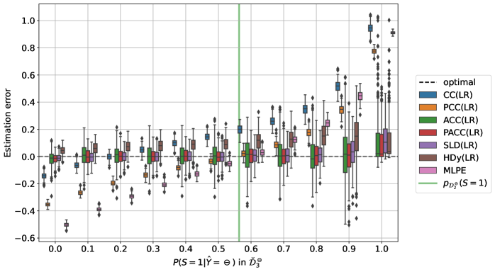
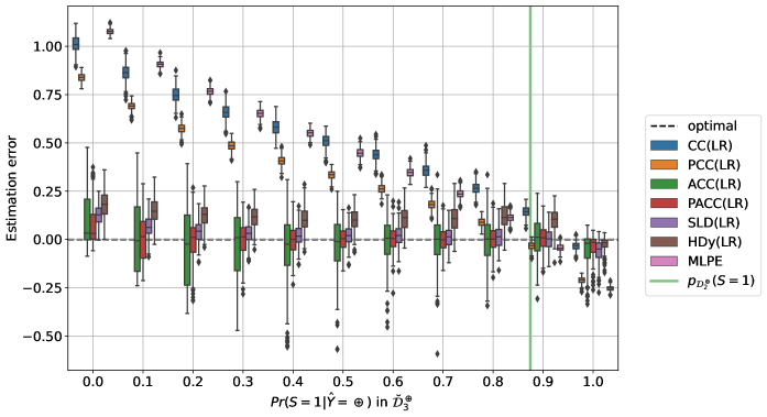
In Figure 1 we report the performance of CC, PCC, ACC, PACC, SLD, HDy, and MLPE on the Adult dataset under the sample-prev-$\mathcal{D}_{3}$ experimental protocol. The estimation error (Equation 16) is reported on the $y$ axis, as we vary the prevalence of the protected group in the test set, which is displayed on the $x$ axis. Figure 1(a) concentrates on prevalence variations in $\mathcal{D}_{3}^{\ominus}$, while Figure 1(b) considers variations of the prevalence of the protected group in $\mathcal{D}_{3}^{\oplus}$. Each boxplot summarizes the results of 5 random splits, 6 role permutations, and 10 samplings of $\breve{\mathcal{D}}_{3}$, for a total of 300 repetitions for each combination of 6 methods and 11 values which vary on the $x$ axis. Boxes enclose the two central quartiles (separated by a median horizontal line), while whiskers surround points in the outer quartiles, except for outliers marked with diamonds.

Similar trends emerge under both sub-protocols. CC, PCC, and MLPE display a clear trend along the $x$ axis, vastly over- or underestimating the demographic disparity of $h$, and proving unreliable in settings where the prevalence values in the unlabelled (test) set shift away from the prevalence values of the training set. In sub-protocol sample-prev-$\mathcal{D}_{3}^{\oplus}$, summarised in Figure 1(b), the prevalence of men ($S=1$) in $\breve{\mathcal{D}}_{3}^{\oplus}$, used to test one of the quantifiers, is almost always lower than the prevalence in the respective training set $\mathcal{D}_{2}^{\oplus}$, reported with a vertical green line. As a result, quantifiers trained on $\mathcal{D}_{2}^{\oplus}$ tend to systematically overestimate the prevalence of males in $\mathcal{D}_{3}^{\oplus}$, thus also overestimating $\mu(1)$ and $\delta_{h}^{S}$, according to Equations (14) and (15). Similar considerations hold for sub-protocol sample-prev-$\mathcal{D}_{3}^{\ominus}$, with a sign flip.

Table 4: Results obtained in the experiments run according to protocol sample-prev-$\mathcal{D}_{3}$.

		$\downarrow$ MAE	$\downarrow$ MSE	$\uparrow$ $P(\mathrm{AE}<0.1)$	$\uparrow$ $P(\mathrm{AE}<0.2)$
Adult	CC(LR)	0.382${}^{\phantom{{\ddagger}}}\pm 0.304$	0.239${}^{\phantom{{\ddagger}}}\pm 0.305$	0.207	0.386
	PCC(LR)	0.299${}^{\phantom{{\ddagger}}}\pm 0.237$	0.146${}^{\phantom{{\ddagger}}}\pm 0.199$	0.235	0.427
	ACC(LR)	0.103${}^{\phantom{{\ddagger}}}\pm 0.097$	0.020${}^{\phantom{{\ddagger}}}\pm 0.047$	0.595	0.870
	PACC(LR)	0.061${}^{\phantom{{\ddagger}}}\pm 0.059$	0.007${}^{\phantom{{\ddagger}}}\pm 0.016$	0.813	0.970
	SLD(LR)	0.055${}^{\phantom{{\ddagger}}}\pm 0.052$	0.006${}^{\phantom{{\ddagger}}}\pm 0.012$	0.846	0.980
	HDy(LR)	0.110${}^{\phantom{{\ddagger}}}\pm 0.079$	0.018${}^{\phantom{{\ddagger}}}\pm 0.032$	0.500	0.893
	MLPE	0.397${}^{\phantom{{\ddagger}}}\pm 0.298$	0.246${}^{\phantom{{\ddagger}}}\pm 0.316$	0.162	0.294
COMPAS	CC(LR)	0.541${}^{\phantom{{\ddagger}}}\pm 0.369$	0.429${}^{\phantom{{\ddagger}}}\pm 0.472$	0.118	0.237
	PCC(LR)	0.337${}^{\phantom{{\ddagger}}}\pm 0.242$	0.172${}^{\phantom{{\ddagger}}}\pm 0.214$	0.181	0.344
	ACC(LR)	0.495${}^{\phantom{{\ddagger}}}\pm 0.363$	0.377${}^{\phantom{{\ddagger}}}\pm 0.471$	0.143	0.252
	PACC(LR)	0.252${}^{\phantom{{\ddagger}}}\pm 0.213$	0.109${}^{\phantom{{\ddagger}}}\pm 0.184$	0.287	0.492
	SLD(LR)	0.169${}^{\phantom{{\ddagger}}}\pm 0.139$	0.048${}^{\phantom{{\ddagger}}}\pm 0.077$	0.385	0.669
	HDy(LR)	0.267${}^{\phantom{{\ddagger}}}\pm 0.213$	0.116${}^{\phantom{{\ddagger}}}\pm 0.176$	0.250	0.472
	MLPE	0.349${}^{\phantom{{\ddagger}}}\pm 0.249$	0.184${}^{\phantom{{\ddagger}}}\pm 0.227$	0.175	0.332
CreditCard	CC(LR)	0.345${}^{\phantom{{\ddagger}}}\pm 0.241$	0.177${}^{\phantom{{\ddagger}}}\pm 0.212$	0.172	0.339
	PCC(LR)	0.325${}^{\phantom{{\ddagger}}}\pm 0.213$	0.151${}^{\phantom{{\ddagger}}}\pm 0.157$	0.176	0.340
	ACC(LR)	0.341${}^{\phantom{{\ddagger}}}\pm 0.259$	0.183${}^{\phantom{{\ddagger}}}\pm 0.256$	0.189	0.367
	PACC(LR)	0.259${}^{\phantom{{\ddagger}}}\pm 0.211$	0.111${}^{\phantom{{\ddagger}}}\pm 0.173$	0.269	0.480
	SLD(LR)	0.190${}^{\phantom{{\ddagger}}}\pm 0.148$	0.058${}^{\phantom{{\ddagger}}}\pm 0.086$	0.334	0.609
	HDy(LR)	0.251${}^{\phantom{{\ddagger}}}\pm 0.190$	0.099${}^{\phantom{{\ddagger}}}\pm 0.142$	0.248	0.478
	MLPE	0.334${}^{\phantom{{\ddagger}}}\pm 0.218$	0.159${}^{\phantom{{\ddagger}}}\pm 0.165$	0.172	0.330

ACC, PACC, SLD and HDy, on the other hand, display low bias, even under sizeable prevalence shift. Their variance is higher than CC and PCC, but their estimation error is moderate overall. The condition $\Pr(S=1|\hat{Y}=\ominus)=1$ (right-most point in Figure 1(a)) is particularly critical for every method due to $p_{\mathcal{D}_{3}}(s=0)$ dropping below 0.1, thus making small estimation errors for the denominator of Equation 15 especially impactful on $\hat{\mu}(0)$.

The results of the COMPAS and CreditCard datasets are reported in Table 4, along with a summary of the results of the Adult dataset we have just discussed. The first and second columns indicate the MAE and MSE values (lower is better), while the third and fourth columns indicate the probability that the Absolute Error (AE) falls below 0.1 and 0.2 across the entire experimental protocol (higher is better). Boldface indicates the best method for a given dataset and metric. The superscripts ${\dagger}$ and ${\ddagger}$ denote the methods (if any) whose error scores (MAE, MSE) are not statistically significantly different from the best according to a paired sample, two-tailed t-test at different confidence levels. Symbol ${\dagger}$ indicates $0.001<p$-value $<0.05$ while symbol ${\ddagger}$ indicates $0.05\leq p$-value; the absence of any such symbol indicates $p$-value $\leq 0.001$ (i.e., that the performance of the method is statistically significantly different from that of the best method). Overall, SLD strikes the best balance between bias and variance. PACC is the second-best approach, outperforming ACC and PCC, demonstrating the utility of combining posterior probabilities and adjustments when the latter can reliably be estimated. The trends we discussed also hold for COMPAS and CreditCard. Note that both datasets appear to provide a setting harder than Adult for the inference of the sensitive attribute $S$ from the non-sensitive attributes $X$.

5.4 Distribution Shift Affecting the Auxiliary Set: Protocol sample-prev-$\mathcal{D}_{2}$

5.4.1 Motivation and Setup

This protocol is analogous to protocol sample-prev-$\mathcal{D}_{3}$ (Section 5.3), but for the fact that it focuses on shifts in the auxiliary set $\mathcal{D}_{2}$, while $\mathcal{D}_{1}$ and $\mathcal{D}_{3}$ remain at their natural prevalence. Similarly to Section 5.3, we assess the signed estimation error under shifts that affect $\mathcal{D}_{2}^{\ominus}$ or $\mathcal{D}_{2}^{\oplus}$, that is, the subsets of $\mathcal{D}_{2}$ labelled positively or negatively by the classifier $h$. Here too, we consider two experimental sub-protocols, describing variations in the prevalence of sensitive attribute $s$ in either subset. More specifically, we let $\Pr(s|\ominus)$ (or its dual $\Pr(s|\oplus)$) take 9 evenly spaced values between 0.1 and 0.9. Pseudocode 3 describes the protocol when acting on $\mathcal{D}_{2}^{\ominus}$; the case for $\mathcal{D}_{2}^{\oplus}$ is analogous, and comes down to swapping the roles of $\mathcal{D}_{2}^{\ominus}$ and $\mathcal{D}_{2}^{\oplus}$ in Lines 3 and 3.

This protocol captures issues of representativity in demographic data, e.g., due to nonuniform response rates across subpopulations (Schouten et al., 2009, 2012). Given the importance of trust for the provision of one’s sensitive attributes, in some domains this provision is considered akin to a data donation (Andrus et al., 2021). Individuals from groups that were historically served with worse quality or had lower acceptance rates for a service can be reluctant to disclose their membership in those groups, fearing that it may be used against them as grounds for rejection or discrimination (Hasnain-Wynia and Baker, 2006). This may be especially true for individuals who perceive to be at high risk of rejection, and this can cause complex selection biases, jointly dependent on $S$ and $Y$, or $S$ and $\hat{Y}$ if individuals have some knowledge of the classification procedure. For example, health care providers may be advised to collect information about the race of patients to monitor the quality of services across subpopulations. In a field study, 28% of patients reported discomfort in revealing their own race to a clerk, with African-American patients significantly less comfortable than white patients on average (Baker et al., 2005).

5.4.2 Results

(a) Protocol sample-prev-$\mathcal{D}_{2}^{\ominus}$

(b) Protocol sample-prev-$\mathcal{D}_{2}^{\oplus}$

Figure 2: Protocol sample-prev-$\mathcal{D}_{2}$ on the Adult dataset. Distribution of the estimation error ($y$ axis) as $\breve{\mathcal{D}}_{2}$ is sampled with a given $\Pr(S=1|Y=\ominus)$ value, plot (a), or $\Pr(S=1|Y=\oplus)$ value, plot (b) ($x$ axis). The green line indicates the value of $\Pr(S=1)$ as observed in $\mathcal{D}_{3}^{\ominus}$, plot (a), or $\mathcal{D}_{3}^{\oplus}$, plot (b).

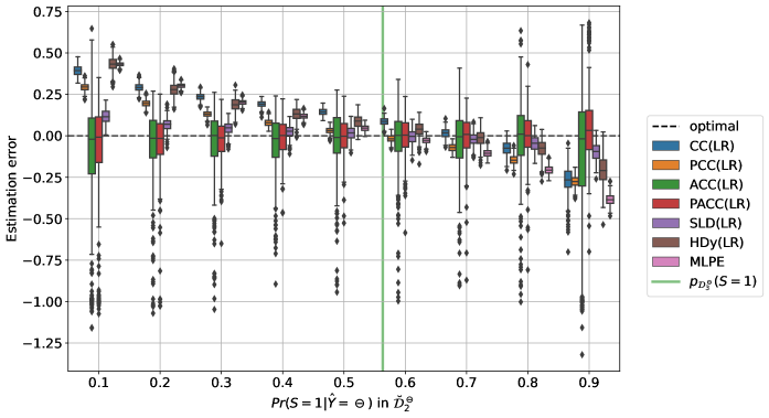
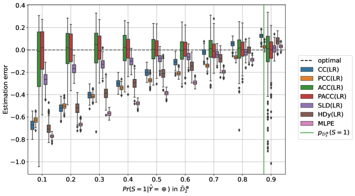
Figure 2 shows the signed estimation error on the $y$ axis, as we vary, on the $x$ axis, the prevalence of the sensitive attribute in $\mathcal{D}_{2}^{\ominus}$ (Figure 2(a)) and $\mathcal{D}_{2}^{\oplus}$ (Figure 2(b)). MLPE, CC, PCC, and HDy prove to be fairly sensitive to shifts in their training set. In sub-protocol sample-prev-$\mathcal{D}_{2}^{\oplus}$, symmetrically to the sub-protocol sample-prev-$\mathcal{D}_{3}^{\oplus}$ discussed in the previous section, the prevalence of males ($S=1$) in subset $\mathcal{D}_{2}^{\oplus}$, used to train one of the quantifiers, is almost always lower than the prevalence in the respective test subset $\mathcal{D}_{3}^{\oplus}$, indicated with a vertical green line. As a result, quantifiers trained on $\mathcal{D}_{2}^{\oplus}$ tend to systematically underestimate the prevalence of males in $\mathcal{D}_{3}^{\oplus}$ and underestimate the (signed) demographic disparity of the classifier $h$.

ACC and PACC require splitting their training set to estimate the respective adjustments (Equations (6)–(9)), and suffer from a reduced cardinality $|\breve{\mathcal{D}}_{2}|=1,000$. Their performance worsens substantially with respect to protocol sample-prev-$\mathcal{D}_{3}$, where $|\mathcal{D}_{2}|>15,000$. Indeed, these methods have been shown to be Fisher-consistent under prior probability shift (Tasche, 2017; Fernandes Vaz et al., 2019), that is, they are guaranteed to be accurate, thanks to the respective adjustments, if $\mathcal{D}_{2}$ is large enough and linked to $\mathcal{D}_{3}$ by prior probability shift. While the latter condition holds, the former is violated under this protocol, hence ACC and PACC are unbiased (in expectation), but display a large variance, due to unstable adjustments. SLD, on the other hand, shows a moderate variance and bias. These effects are especially evident at the extremes of the $x$ axis, which correspond to settings where few instances with either $S=0$ or $S=1$ are available for quantifier training. In turn, the few positives (negatives) make it particularly difficult to reliably estimate $\mathrm{tpr}_{k_{s}}$ ($\mathrm{tnr}_{k_{s}}$), as required by Equations 7 and 9. For example, in Figure 2(a) we see that the error of ACC ranges between $-1.3$ and $0.7$. Given that the true demographic disparity of the classifier $h$ is $\delta_{h}^{S}=0.3$, these are the worst possible errors, corresponding to extreme estimates $\hat{\delta_{h}^{S}}=-1$ and $\hat{\delta_{h}^{S}}=1$, respectively. Finally, it is worth noting that PACC outperforms ACC, thanks to efficient use of posteriors $\pi_{s}(\mathbf{x}_{i})$ in place of binary decisions $k_{s}(\mathbf{x}_{i})$.

Table 5: Results obtained in the experiments run according to protocol sample-prev-$\mathcal{D}_{2}$.

		$\downarrow$ MAE	$\downarrow$ MSE	$\uparrow$ $P(\mathrm{AE}<0.1)$	$\uparrow$ $P(\mathrm{AE}<0.2)$
Adult	CC(LR)	0.230${}^{\phantom{{\ddagger}}}\pm 0.177$	0.084${}^{\phantom{{\ddagger}}}\pm 0.118$	0.274	0.523
	PCC(LR)	0.213${}^{\phantom{{\ddagger}}}\pm 0.169$	0.074${}^{\phantom{{\ddagger}}}\pm 0.103$	0.323	0.551
	ACC(LR)	0.159${}^{\phantom{{\ddagger}}}\pm 0.178$	0.057${}^{\phantom{{\ddagger}}}\pm 0.159$	0.439	0.789
	PACC(LR)	0.112${}^{\phantom{{\ddagger}}}\pm 0.118$	0.026${}^{\phantom{{\ddagger}}}\pm 0.093$	0.559	0.889
	SLD(LR)	0.081${}^{\phantom{{\ddagger}}}\pm 0.070$	0.011${}^{\phantom{{\ddagger}}}\pm 0.020$	0.705	0.929
	HDy(LR)	0.219${}^{\phantom{{\ddagger}}}\pm 0.188$	0.084${}^{\phantom{{\ddagger}}}\pm 0.128$	0.345	0.573
	MLPE	0.295${}^{\phantom{{\ddagger}}}\pm 0.218$	0.134${}^{\phantom{{\ddagger}}}\pm 0.165$	0.239	0.410
COMPAS	CC(LR)	0.498${}^{\phantom{{\ddagger}}}\pm 0.253$	0.312${}^{\phantom{{\ddagger}}}\pm 0.260$	0.044	0.128
	PCC(LR)	0.264${}^{\phantom{{\ddagger}}}\pm 0.186$	0.104${}^{\phantom{{\ddagger}}}\pm 0.126$	0.227	0.431
	ACC(LR)	0.469${}^{\phantom{{\ddagger}}}\pm 0.276$	0.296${}^{\phantom{{\ddagger}}}\pm 0.303$	0.080	0.184
	PACC(LR)	0.338${}^{\phantom{{\ddagger}}}\pm 0.254$	0.179${}^{\phantom{{\ddagger}}}\pm 0.250$	0.185	0.356
	SLD(LR)	0.160${}^{\phantom{{\ddagger}}}\pm 0.123$	0.041${}^{\phantom{{\ddagger}}}\pm 0.060$	0.386	0.678
	HDy(LR)	0.255${}^{\phantom{{\ddagger}}}\pm 0.189$	0.101${}^{\phantom{{\ddagger}}}\pm 0.135$	0.246	0.463
	MLPE	0.275${}^{\phantom{{\ddagger}}}\pm 0.193$	0.112${}^{\phantom{{\ddagger}}}\pm 0.134$	0.219	0.417
CreditCard	CC(LR)	0.429${}^{\phantom{{\ddagger}}}\pm 0.252$	0.248${}^{\phantom{{\ddagger}}}\pm 0.236$	0.103	0.225
	PCC(LR)	0.204${}^{\phantom{{\ddagger}}}\pm 0.140$	0.061${}^{\phantom{{\ddagger}}}\pm 0.073$	0.287	0.551
	ACC(LR)	0.535${}^{\phantom{{\ddagger}}}\pm 0.316$	0.387${}^{\phantom{{\ddagger}}}\pm 0.353$	0.085	0.165
	PACC(LR)	0.512${}^{\phantom{{\ddagger}}}\pm 0.311$	0.359${}^{\phantom{{\ddagger}}}\pm 0.343$	0.094	0.171
	SLD(LR)	0.171${}^{\phantom{{\ddagger}}}\pm 0.123$	0.044${}^{\phantom{{\ddagger}}}\pm 0.058$	0.348	0.645
	HDy(LR)	0.222${}^{\phantom{{\ddagger}}}\pm 0.159$	0.074${}^{\phantom{{\ddagger}}}\pm 0.101$	0.260	0.508
	MLPE	0.210${}^{\phantom{{\ddagger}}}\pm 0.143$	0.065${}^{\phantom{{\ddagger}}}\pm 0.077$	0.280	0.536

These trends also hold for COMPAS and CreditCard, as summarized in Table 5. Similarly to Table 4, we find that, under large shifts between the auxiliary and the test set, the estimation of demographic disparity is more difficult on COMPAS and CreditCard than on Adult. Overall, these experiments show that CC and PCC fare poorly under prior probability shift, and are outperformed by estimators with better theoretical guarantees.

5.5 Reduced Cardinality of the Auxiliary Set: Protocol sample-size-$\mathcal{D}_{2}$

5.5.1 Motivation and Setup

In this experimental protocol, we focus on the size of the auxiliary set $\mathcal{D}_{2}$, studying its influence on the estimation problem. Our goal is to understand how small this set can be before degrading the performance of our estimation techniques. We use subsets $\breve{\mathcal{D}}_{2}$ of the auxiliary set, obtained by sampling instances uniformly without replacement from it. We let their cardinality $|\breve{\mathcal{D}}_{2}|$ take five values evenly spaced on a logarithmic scale, between a minimum size $|\breve{\mathcal{D}}_{2}|$=1,000 and a maximum size $|\breve{\mathcal{D}}_{2}|=|\mathcal{D}_{2}|$. In other words, we let the cardinality of the auxiliary set take five different values between 1,000 and $|\mathcal{D}_{2}|$ in a geometric progression.

This protocol is justified by the well-documented difficulties in the acquisition of demographic data for industry professionals, which vary depending on the domain, the company and other factors of disparate nature (Beutel et al., 2019b; Holstein et al., 2019; Galdon Clavell et al., 2020; Bogen et al., 2020; Andrus et al., 2021). As an example, Galdon Clavell et al. (2020) perform an internal fairness audit of a personalized wellness recommendation app, for which sensitive features are not collected during production, following the principles of data minimization. However, sensitive features were available in a previously obtained auxiliary set. Furthermore, in the US, the collection of sensitive attributes is highly industry dependent, ranging from mandatory to forbidden, depending on the fragmented regulation applicable in each domain (Bogen et al., 2020). High-quality auxiliary sets can be obtained through optional surveys (Wilson et al., 2021), for which response rates are highly dependent on trust, and can be improved by making the intended use of the data clearer (Andrus et al., 2021), directly impacting the cardinality of $\mathcal{D}_{2}$.

Therefore, the cardinality of the auxiliary set $\mathcal{D}_{2}$ is an interesting variable in the context of fairness audits. The estimation methods that we consider have peculiar data requirements, such as the need to estimate true/false positive rates. For this reason, interesting patterns should emerge from this protocol. We expect key trends for the estimation error to vary monotonically with $|\breve{\mathcal{D}}_{2}|$, which is why we let it vary according to a geometric progression.

5.5.2 Results

The signed estimation error on the Adult dataset under this experimental protocol is illustrated in Figure 3, as we vary the cardinality $|\breve{\mathcal{D}}_{2}|$ along the $x$ axis. Clearly, the variance for each approach decreases as the size of $\breve{\mathcal{D}}_{2}$ increases. Additionally, slight biases may improve, as is the case with HDy, whose median error approaches zero as $|\breve{\mathcal{D}}_{2}|$ increases. These trends are a direct confirmation of hints already obtained from the protocols discussed above. The most striking trend is the unreliability of ACC and PACC (and especially the former) in the small data regime.

Figure 3: Protocol sample-size-$\mathcal{D}_{2}$ on the Adult dataset. Distribution of the estimation error ($y$ axis) as the cardinality $|\breve{\mathcal{D}}_{2}|$ is varied ($x$ axis).

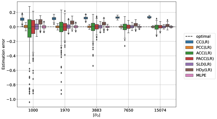
Similar results are obtained for COMPAS and CreditCard, as reported in Table 6. Across the three datasets, PACC and ACC perform quite poorly due to the difficulty in estimating $\mathrm{tpr}_{k_{s}}$ and $\mathrm{fpr}_{k_{s}}$ with the few labelled data points available from $\breve{\mathcal{D}}_{2}$. On the other hand, both SLD and HDy are fairly reliable. PCC and MLPE stand out as strong performers, with low bias and low variance. This is due to the fact that, under this experimental protocol, there is no shift between the auxiliary set $\mathcal{D}_{2}$, on which the quantifiers are trained, and the test set $\mathcal{D}_{3}$, on which they are tested. Since the current protocol focuses on the cardinality of the auxiliary set, $\mathcal{D}_{2}$ and $\mathcal{D}_{3}$ remain stratified subsets of the Adult dataset, with identical distributions over $(S,Y)$. In turn, this favours MLPE, which assumes no shift between $\mathcal{D}_{2}$ and $\mathcal{D}_{3}$, and PCC, which relies on the fact that the posterior probabilities of its underlying classifier $k$ are well-calibrated on $\mathcal{D}_{3}$.

Table 6: Results obtained in the experiments run according to protocol sample-size-$\mathcal{D}_{2}$

		$\downarrow$ MAE	$\downarrow$ MSE	$\uparrow$ $P(\mathrm{AE}<0.1)$	$\uparrow$ $P(\mathrm{AE}<0.2)$
Adult	CC(LR)	0.120${}^{\phantom{{\ddagger}}}\pm 0.022$	0.015${}^{\phantom{{\ddagger}}}\pm 0.005$	0.159	1.000
	PCC(LR)	0.012${}^{\phantom{{\ddagger}}}\pm 0.010$	0.000${}^{\phantom{{\ddagger}}}\pm 0.000$	1.000	1.000
	ACC(LR)	0.083${}^{\phantom{{\ddagger}}}\pm 0.113$	0.020${}^{\phantom{{\ddagger}}}\pm 0.082$	0.747	0.928
	PACC(LR)	0.055${}^{\phantom{{\ddagger}}}\pm 0.079$	0.009${}^{\phantom{{\ddagger}}}\pm 0.048$	0.856	0.969
	SLD(LR)	0.025${}^{\phantom{{\ddagger}}}\pm 0.020$	0.001${}^{\phantom{{\ddagger}}}\pm 0.002$	0.996	1.000
	HDy(LR)	0.047${}^{\phantom{{\ddagger}}}\pm 0.033$	0.003${}^{\phantom{{\ddagger}}}\pm 0.004$	0.922	1.000
	MLPE	0.013${}^{{\ddagger}}\pm 0.012$	0.000${}^{{\dagger}}\pm 0.001$	1.000	1.000
COMPAS	CC(LR)	0.353${}^{\phantom{{\ddagger}}}\pm 0.047$	0.127${}^{\phantom{{\ddagger}}}\pm 0.032$	0.000	0.005
	PCC(LR)	0.030${}^{{\ddagger}}\pm 0.020$	0.001${}^{\phantom{{\ddagger}}}\pm 0.001$	0.999	1.000
	ACC(LR)	0.381${}^{\phantom{{\ddagger}}}\pm 0.213$	0.190${}^{\phantom{{\ddagger}}}\pm 0.214$	0.097	0.186
	PACC(LR)	0.265${}^{\phantom{{\ddagger}}}\pm 0.212$	0.115${}^{\phantom{{\ddagger}}}\pm 0.183$	0.247	0.467
	SLD(LR)	0.135${}^{\phantom{{\ddagger}}}\pm 0.098$	0.028${}^{\phantom{{\ddagger}}}\pm 0.038$	0.441	0.765
	HDy(LR)	0.108${}^{\phantom{{\ddagger}}}\pm 0.082$	0.018${}^{\phantom{{\ddagger}}}\pm 0.027$	0.549	0.858
	MLPE	0.029${}^{\phantom{{\ddagger}}}\pm 0.021$	0.001${}^{{\ddagger}}\pm 0.002$	0.999	1.000
CreditCard	CC(LR)	0.177${}^{\phantom{{\ddagger}}}\pm 0.078$	0.037${}^{\phantom{{\ddagger}}}\pm 0.030$	0.177	0.629
	PCC(LR)	0.016${}^{{\ddagger}}\pm 0.013$	0.000${}^{{\ddagger}}\pm 0.001$	1.000	1.000
	ACC(LR)	0.337${}^{\phantom{{\ddagger}}}\pm 0.266$	0.184${}^{\phantom{{\ddagger}}}\pm 0.259$	0.203	0.368
	PACC(LR)	0.299${}^{\phantom{{\ddagger}}}\pm 0.255$	0.154${}^{\phantom{{\ddagger}}}\pm 0.240$	0.261	0.445
	SLD(LR)	0.053${}^{\phantom{{\ddagger}}}\pm 0.043$	0.005${}^{\phantom{{\ddagger}}}\pm 0.008$	0.871	0.985
	HDy(LR)	0.057${}^{\phantom{{\ddagger}}}\pm 0.046$	0.005${}^{\phantom{{\ddagger}}}\pm 0.009$	0.831	0.991
	MLPE	0.016${}^{\phantom{{\ddagger}}}\pm 0.013$	0.000${}^{\phantom{{\ddagger}}}\pm 0.001$	1.000	1.000

5.6 Distribution Shift Affecting $\mathcal{D}_{1}$: Protocol sample-prev-$\mathcal{D}_{1}$

5.6.1 Motivation and Setup

With this protocol we evaluate the impact of shifts in the training set $\mathcal{D}_{1}$, by drawing different subsets $\breve{\mathcal{D}}_{1}$ as we vary $\Pr(Y=S)$. More specifically, we vary $\Pr(Y=S)$ between 0 and 1 with a step of 0.1. In other words, we sample at random from $\mathcal{D}_{1}$ a proportion $p$ of instances $(\mathbf{x}_{i},s_{i},y_{i})$ such that $Y=S$ and a proportion $(1-p)$ such that $Y\neq S$, with $p\in\left\{0.0,0.1,\dots,0.9,1.0\right\}$. We choose a limited cardinality $|\breve{\mathcal{D}}_{1}|=500$, which allows us to perform multiple repetitions at reasonable computational costs, as described in Section 5.1. Although this may impact the quality of the classifier $h$, this aspect is not the central focus of the present work.

This experimental protocol aligns with biased data collection procedures, sometimes referred to as censored data (Kallus and Zhou, 2018). Indeed, it is common for the ground-truth variable to represent a mere proxy for the actual quantity of interest, with nontrivial sampling effects between the two. For example, the validity of arrest data as a proxy for offence has been brought into question (Fogliato et al., 2021). In fact, in this domain, different sources of sampling bias can be in action, such as uneven allocation of police resources between jurisdictions and neighbourhoods (Holmes et al., 2008) and lower levels of cooperation in populations who feel oppressed by law enforcement (Xie and Lauritsen, 2012).

By varying $\Pr(Y=S)$ we impose a spurious correlation between $Y$ and $S$, which may be picked up by the classifier $h$. In extreme situations, such as when $\Pr(Y=S)\simeq 1$, a classifier $h$ can confound the concepts behind $S$ and $Y$. In turn, we expect this to unevenly affect the acceptance rates for the two demographic groups, effectively changing the demographic disparity of $h$, i.e., our estimand $\delta_{h}^{S}$. Pseudocode 5 describes the main steps to implement Protocol sample-prev-$\mathcal{D}_{1}$.

5.6.2 Results

Figure 4: Protocol sample-prev-$\mathcal{D}_{1}$ on the Adult dataset. Distribution of the estimation error ($y$ axis) as $\breve{\mathcal{D}}_{1}$ is sampled with a given $\Pr(Y=S)$ ($x$ axis). Each boxplot summarizes the results of 5 random splits, 6 role permutations and 10 samplings of $\breve{\mathcal{D}}_{1}$.

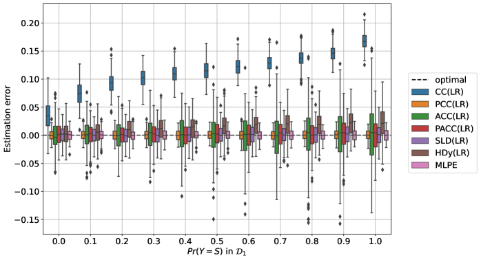
In Figure 4, the $y$ axis depicts the estimation error (Equation 16), as we vary $\Pr(Y=S)$ along the $x$ axis. Each quantification approach outperforms vanilla CC, which overestimates the demographic disparity of the classifier $h$, i.e., its estimate is larger than the ground truth value, so $\hat{\delta}_{h}^{S,\text{CC}}>\delta_{h}^{S}$. ACC, PCC, PACC, SLD, HDy, and MLPE display a negligible bias and a reliable estimate of demographic disparity. The absolute error for these techniques is always below 0.1, except for a few outliers.

Table 7: Results obtained in the experiments run according to protocol sample-prev-$\mathcal{D}_{1}$.

		$\downarrow$ MAE	$\downarrow$ MSE	$\uparrow$ $P(\mathrm{AE}<0.1)$	$\uparrow$ $P(\mathrm{AE}<0.2)$
Adult	CC(LR)	0.112${}^{\phantom{{\ddagger}}}\pm 0.038$	0.014${}^{\phantom{{\ddagger}}}\pm 0.008$	0.321	0.998
	PCC(LR)	0.008${}^{\phantom{{\ddagger}}}\pm 0.005$	0.000${}^{\phantom{{\ddagger}}}\pm 0.000$	1.000	1.000
	ACC(LR)	0.029${}^{\phantom{{\ddagger}}}\pm 0.024$	0.001${}^{\phantom{{\ddagger}}}\pm 0.003$	0.983	1.000
	PACC(LR)	0.019${}^{\phantom{{\ddagger}}}\pm 0.014$	0.001${}^{\phantom{{\ddagger}}}\pm 0.001$	1.000	1.000
	SLD(LR)	0.013${}^{\phantom{{\ddagger}}}\pm 0.010$	0.000${}^{\phantom{{\ddagger}}}\pm 0.000$	1.000	1.000
	HDy(LR)	0.022${}^{\phantom{{\ddagger}}}\pm 0.016$	0.001${}^{\phantom{{\ddagger}}}\pm 0.001$	1.000	1.000
	MLPE	0.008${}^{\phantom{{\ddagger}}}\pm 0.006$	0.000${}^{\phantom{{\ddagger}}}\pm 0.000$	1.000	1.000
COMPAS	CC(LR)	0.328${}^{\phantom{{\ddagger}}}\pm 0.091$	0.116${}^{\phantom{{\ddagger}}}\pm 0.056$	0.022	0.081
	PCC(LR)	0.026${}^{\phantom{{\ddagger}}}\pm 0.019$	0.001${}^{\phantom{{\ddagger}}}\pm 0.001$	1.000	1.000
	ACC(LR)	0.349${}^{\phantom{{\ddagger}}}\pm 0.211$	0.166${}^{\phantom{{\ddagger}}}\pm 0.192$	0.130	0.252
	PACC(LR)	0.194${}^{\phantom{{\ddagger}}}\pm 0.164$	0.065${}^{\phantom{{\ddagger}}}\pm 0.115$	0.345	0.607
	SLD(LR)	0.114${}^{\phantom{{\ddagger}}}\pm 0.083$	0.020${}^{\phantom{{\ddagger}}}\pm 0.027$	0.512	0.849
	HDy(LR)	0.096${}^{\phantom{{\ddagger}}}\pm 0.076$	0.015${}^{\phantom{{\ddagger}}}\pm 0.023$	0.605	0.897
	MLPE	0.027${}^{{\ddagger}}\pm 0.019$	0.001${}^{{\ddagger}}\pm 0.001$	1.000	1.000
CreditCard	CC(LR)	0.152${}^{\phantom{{\ddagger}}}\pm 0.095$	0.032${}^{\phantom{{\ddagger}}}\pm 0.036$	0.338	0.711
	PCC(LR)	0.010${}^{\phantom{{\ddagger}}}\pm 0.007$	0.000${}^{\phantom{{\ddagger}}}\pm 0.000$	1.000	1.000
	ACC(LR)	0.187${}^{\phantom{{\ddagger}}}\pm 0.152$	0.058${}^{\phantom{{\ddagger}}}\pm 0.094$	0.347	0.626
	PACC(LR)	0.130${}^{\phantom{{\ddagger}}}\pm 0.106$	0.028${}^{\phantom{{\ddagger}}}\pm 0.046$	0.487	0.777
	SLD(LR)	0.047${}^{\phantom{{\ddagger}}}\pm 0.037$	0.004${}^{\phantom{{\ddagger}}}\pm 0.005$	0.902	0.998
	HDy(LR)	0.061${}^{\phantom{{\ddagger}}}\pm 0.047$	0.006${}^{\phantom{{\ddagger}}}\pm 0.009$	0.814	0.989
	MLPE	0.011${}^{\phantom{{\ddagger}}}\pm 0.008$	0.000${}^{\phantom{{\ddagger}}}\pm 0.000$	1.000	1.000

Results for the COMPAS and CreditCard datasets are reported in Table 7. Confirming the results of previous protocols, these datasets provide a harder setting for the estimate of demographic disparity, as shown by higher MAE and MSE, which, for instance, increase by one order of magnitude for SLD and PACC moving from Adult to COMPAS. PCC is the best performer, for the same reasons discussed in Section 5.3, i.e., the absence of shift between $\mathcal{D}_{2}$ and $\mathcal{D}_{3}$.

5.7 Distribution Shift Affecting $\mathcal{D}_{1}$: Protocol flip-prev-$\mathcal{D}_{1}$

5.7.1 Motivation and Setup

Certain biases in the training set resulting from domain-specific practices, such as the use of arrest as a substitute for the offence, can be modelled as either a selection bias (Fogliato et al., 2021) or a label bias distorting the ground truth variable $Y$ (Fogliato et al., 2020). With this experimental protocol, we impose the latter bias by actively flipping some ground truth labels $Y$ in $\mathcal{D}_{1}$ based on their sensitive attribute. Similarly to sample-prev-$\mathcal{D}_{1}$, this protocol achieves a given association between the target $Y$ and the sensitive variable $S$ in the training set $\mathcal{D}_{1}$. However, instead of sampling, it does so by flipping the $Y$ label of some data points. More specifically, we impose $\Pr(Y=\ominus|S=0)=\Pr(Y=\oplus|S=1)=p$ and let $p$ take values across eleven evenly spaced values between 0 and 1. For every value of $p$, we first sample a random subset $\breve{\mathcal{D}}_{1}$ of the training set with cardinality 500. Next, we actively flip some $Y$ labels in both demographic groups, until both $\Pr(Y=\ominus|S=0)$ and $\Pr(Y=\oplus|S=1)$ reach the desired value of $p\in\left\{0.0,0.1,\dots,0.9,1.0\right\}$. Finally, we train a classifier $h$ on the attributes $X$ and modified ground truth $Y$ of $\breve{\mathcal{D}}_{1}$.

This experimental protocol is compatible with settings where the training data capture a distorted ground truth due to systematic biases and group-dependent annotation accuracy (Wang et al., 2021a). As an example, the quality of medical diagnoses can depend on race, sex, and socioeconomic status (Gianfrancesco et al., 2018). In addition, health care expenditures have been used as a proxy to train an algorithm deployed nationwide in the US to estimate patients’ health care needs, resulting in a systematic underestimation of the needs of African-American patients (Obermeyer et al., 2019). In the hiring domain, employer response rates to resumes have been found to vary with the perceived ethnic origin of an applicant’s name (Bertrand and Mullainathan, 2004). These are all examples where the “ground truth” associated with a dataset is distorted to the disadvantage of a sensitive demographic group.

Similarly to Section 5.6, we expect that this experimental protocol will cause significant variations in the demographic disparity of the classifier $h$ due to the strong correlation we impose between $S$ and $Y$ by label flipping. The pseudocode that describes this protocol is essentially the same as in Pseudocode 5, simply replacing the sampling in line 5 with the label flipping procedure described above; therefore, we omit it.

5.7.2 Results

Figure 5: Protocol flip-prev-$\mathcal{D}_{1}$ on the Adult dataset. Distribution of the estimation error ($y$ axis) as $\delta_{h}^{S}$ varies ($x$ axis).

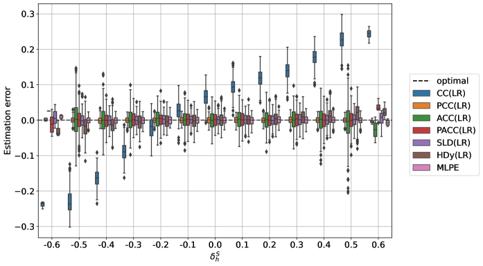
Figure 5 illustrates the key trends caused by this experimental protocol on the Adult dataset. A clear trend is visible along the $x$ axis, which reports the true demographic disparity $\delta_{h}^{S}$ for the classifier $h$ (Equation 10), quantized with a step of 0.1. We choose to depict the true demographic disparity on the $x$ axis as it is the estimand, hence a quantity of interest by definition. The error incurred by CC displays a linear trend that goes from severe underestimation (for low values of the $x$ axis) to severe overestimation (for large values of the $x$ axis). In other words, the (signed) estimation error increases with the true demographic disparity of the classifier $h$, a phenomenon also noticed by Chen et al. (2019). All remaining approaches compensate for this weakness and display a good estimation error: PCC, ACC, PACC, SLD, HDy, and MLPE have low variance and a median estimation close to zero across different values of the estimand. Table 8 summarizes similar results on COMPASS and CreditCard; PCC remains well-calibrated and very effective, while SLD and HDy also have good performance.

Table 8: Results obtained in the experiments run according to protocol flip-prev-$\mathcal{D}_{1}$.

		$\downarrow$ MAE	$\downarrow$ MSE	$\uparrow$ $P(\mathrm{AE}<0.1)$	$\uparrow$ $P(\mathrm{AE}<0.2)$
Adult	CC(LR)	0.151${}^{\phantom{{\ddagger}}}\pm 0.072$	0.028${}^{\phantom{{\ddagger}}}\pm 0.021$	0.274	0.706
	PCC(LR)	0.008${}^{\phantom{{\ddagger}}}\pm 0.006$	0.000${}^{\phantom{{\ddagger}}}\pm 0.000$	1.000	1.000
	ACC(LR)	0.030${}^{\phantom{{\ddagger}}}\pm 0.025$	0.002${}^{\phantom{{\ddagger}}}\pm 0.003$	0.982	0.999
	PACC(LR)	0.020${}^{\phantom{{\ddagger}}}\pm 0.015$	0.001${}^{\phantom{{\ddagger}}}\pm 0.001$	1.000	1.000
	SLD(LR)	0.014${}^{\phantom{{\ddagger}}}\pm 0.011$	0.000${}^{\phantom{{\ddagger}}}\pm 0.000$	1.000	1.000
	HDy(LR)	0.022${}^{\phantom{{\ddagger}}}\pm 0.017$	0.001${}^{\phantom{{\ddagger}}}\pm 0.001$	1.000	1.000
	MLPE	0.009${}^{\phantom{{\ddagger}}}\pm 0.006$	0.000${}^{\phantom{{\ddagger}}}\pm 0.000$	1.000	1.000
COMPAS	CC(LR)	0.388${}^{\phantom{{\ddagger}}}\pm 0.116$	0.164${}^{\phantom{{\ddagger}}}\pm 0.083$	0.027	0.068
	PCC(LR)	0.027${}^{\phantom{{\ddagger}}}\pm 0.020$	0.001${}^{\phantom{{\ddagger}}}\pm 0.001$	0.998	1.000
	ACC(LR)	0.392${}^{\phantom{{\ddagger}}}\pm 0.211$	0.198${}^{\phantom{{\ddagger}}}\pm 0.199$	0.105	0.194
	PACC(LR)	0.195${}^{\phantom{{\ddagger}}}\pm 0.160$	0.063${}^{\phantom{{\ddagger}}}\pm 0.106$	0.337	0.611
	SLD(LR)	0.115${}^{\phantom{{\ddagger}}}\pm 0.084$	0.020${}^{\phantom{{\ddagger}}}\pm 0.027$	0.513	0.836
	HDy(LR)	0.094${}^{\phantom{{\ddagger}}}\pm 0.075$	0.015${}^{\phantom{{\ddagger}}}\pm 0.023$	0.612	0.906
	MLPE	0.028${}^{{\ddagger}}\pm 0.019$	0.001${}^{{\ddagger}}\pm 0.001$	0.999	1.000
CreditCard	CC(LR)	0.159${}^{\phantom{{\ddagger}}}\pm 0.101$	0.036${}^{\phantom{{\ddagger}}}\pm 0.037$	0.345	0.640
	PCC(LR)	0.011${}^{\phantom{{\ddagger}}}\pm 0.009$	0.000${}^{\phantom{{\ddagger}}}\pm 0.000$	1.000	1.000
	ACC(LR)	0.223${}^{\phantom{{\ddagger}}}\pm 0.185$	0.084${}^{\phantom{{\ddagger}}}\pm 0.130$	0.307	0.565
	PACC(LR)	0.147${}^{\phantom{{\ddagger}}}\pm 0.117$	0.035${}^{\phantom{{\ddagger}}}\pm 0.056$	0.420	0.725
	SLD(LR)	0.056${}^{\phantom{{\ddagger}}}\pm 0.043$	0.005${}^{\phantom{{\ddagger}}}\pm 0.007$	0.843	0.995
	HDy(LR)	0.071${}^{\phantom{{\ddagger}}}\pm 0.055$	0.008${}^{\phantom{{\ddagger}}}\pm 0.012$	0.732	0.973
	MLPE	0.012${}^{{\dagger}}\pm 0.009$	0.000${}^{{\dagger}}\pm 0.000$	1.000	1.000

5.8 Estimating Fairness for Discrimination-Aware Classifiers

5.8.1 Motivation and Setup

So far, we have considered classifiers $h(\mathbf{x})$ which only maximize accuracy. In practice, it can be especially interesting to monitor fairness for methods that target this quantity, explicitly optimizing fairness during training. In fact, sensitive attributes may be available during training, allowing for a direct optimization of equity, but unavailable after deployment, complicating fairness evaluation of live systems. In this section, we replace the vanilla LR classifier from the previous experiments with a fairness-aware method. We train a decision tree $h_{\mathrm{T}}$, jointly optimizing accuracy and demographic parity, with the cost-sensitive method of Agarwal et al. (2018). This method makes use of $s$ during training to adjust the cost of positive and negative predictions according to group membership. This learning scheme leads to a classifier $h_{\mathrm{T}}(\mathbf{x})$ which is fairness-aware but does not require access to sensitive attributes to issue predictions on $\mathcal{D}_{3}$.

5.8.2 Results

(a) Protocol sample-prev-$\mathcal{D}_{3}^{\ominus}$

(b) Protocol sample-prev-$\mathcal{D}_{3}^{\oplus}$

Figure 6: Experiments conducted according to protocol sample-prev-$\mathcal{D}_{3}$ on a fairness-aware classifier.

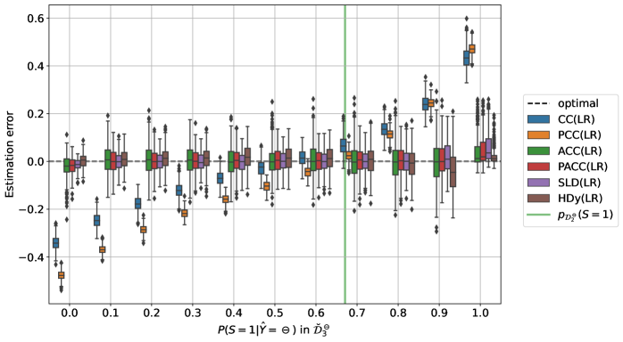
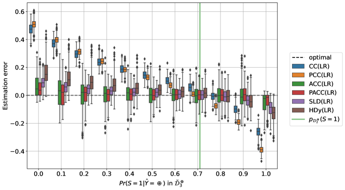
We focus our exposition on protocol sample-prev-$\mathcal{D}_{3}$; analogous results are obtained on the remaining protocols. The fairness-aware decision tree improves DD by one order of magnitude, with an average $\delta_{h_{\mathrm{T}}}^{S}=0.017$, down from $\delta_{h}^{S}=0.158$ for LR. Figure 6, reporting the estimation error from different quantifiers, shows the same patterns as its counterpart from Figure 1. CC and PCC have a sizeable bias, while ACC, PACC, SLD, and HDy display low estimation error for all the tested prevalence values. This experiment confirms the suitability of our method in measuring fairness under unawareness, also for fairness-aware classifiers.

5.9 Quantifying Without Classifying

5.9.1 Motivation and Setup

The motivating use case for this work are internal audits of group fairness, to characterize a model and its potential to harm sensitive categories of users. Following Awasthi et al. (2021), we envision this as an important first step in empowering practitioners to argue for resources and, more broadly, to advocate for a deeper understanding and careful evaluation of models. Unfortunately, developing a tool to infer demographic information, even if motivated by careful intentions and good faith, leaves open the possibility for misuse, especially at an individual level. Once a predictive tool, also capable of instance-level classification, is available, it will be tempting for some actors to exploit it precisely for this purpose.

For example, the Bayesian Improved Surname Geocoding (BISG) method was designed to estimate population-level disparities in health care (Elliott et al., 2009), but later used to identify individuals potentially eligible for settlements related to discriminatory practices of auto lenders (Andriotis and Ensign, 2015; Koren, 2016). Automatic inference of sensitive attributes of individuals is problematic for several reasons. Such procedure exploits the co-occurrence of membership in a group and display of a given trait, running the risk of learning, encoding, and reinforcing stereotypical associations. Although also true of group-level estimates, this practice is particularly troublesome at the individual level, where it is likely to cause harms for people who do not fit the norm, resulting, for instance, in misgendering and the associated negative effects (McLemore, 2015). Even when “accurate”, the mere act of externally assigning sensitive labels can be problematic. For example, gender assignment can be forceful and cause psychological harm for individuals (Keyes, 2018).

In this section, we aim to demonstrate that it is possible to decouple the objective of (group-level) quantification of sensitive attributes from that of (individual-level) classification. For each protocol in the previous sections, we compute the accuracy and $F_{1}$ score (defined below) of the sensitive attribute classifier $k$ underlying the tested quantifiers, comparing it against their estimation error for class prevalence of the same sensitive attribute (Equation 16). Accuracy is the proportion of correctly classified instances over the total (Equation 19) while $F_{1}$ is the harmonic mean of precision and recall (Equation 22). Both measures can be computed from the counters of true positives (TP), true negatives (TN), false positives (FP), and false negatives (FN), as follows:

$$\mathrm{accuracy}= \ \dfrac{\mathrm{TP}+\mathrm{TN}}{\mathrm{TP}+\mathrm{TN}+\mathrm{FP}+\mathrm{FN}}$$ (19)

$$F_{1}= \ \left\{\begin{array}[]{cl}\dfrac{2\mathrm{TP}}{2\mathrm{TP}+\mathrm{FP}+\mathrm{FN}}&\mathrm{if}\ \mathrm{TP}+\mathrm{FP}+\mathrm{FN}>0\rule[-12.91663pt]{0.0pt}{30.1388pt}\\ 1&\mathrm{if}\ \mathrm{TP}=\mathrm{FP}=\mathrm{FN}=0\\ \end{array}\right.$$ (22)

5.9.2 Results

(a) Protocol sample-prev-$\mathcal{D}_{2}^{\ominus}$

(b) Protocol sample-prev-$\mathcal{D}_{2}^{\oplus}$

Figure 7: Performance of CC, SLD and PACC on the Adult dataset when used for quantification (MAE – lower is better, dashed) and classification ($F_{1}$, accuracy – higher is better, solid) under protocol sample-prev-$\mathcal{D}_{2}$. The classification performance of PACC is equivalent to that of CC (both equal to the performance of the underlying LR), and we thus omit it for readability.

(a) Protocol sample-prev-$\mathcal{D}_{3}^{\ominus}$

(b) Protocol sample-prev-$\mathcal{D}_{3}^{\oplus}$

Figure 8: Performance of CC, SLD and PACC on the Adult dataset when used for quantification (MAE – lower is better, dashed) and classification ($F_{1}$, accuracy – higher is better, solid) under protocol sample-prev-$\mathcal{D}_{3}$. The classification performance of PACC is equivalent to that of CC (both equal to the performance of the underlying LR), and we thus omit it for readability.

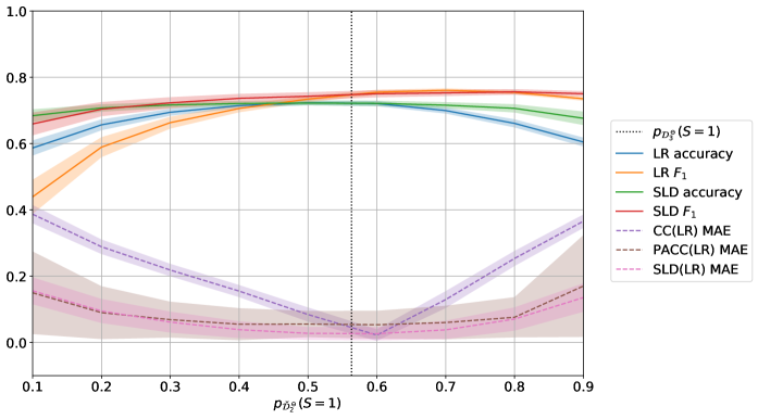
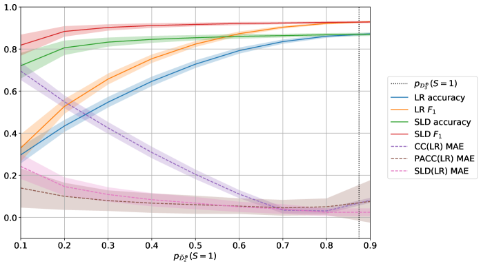
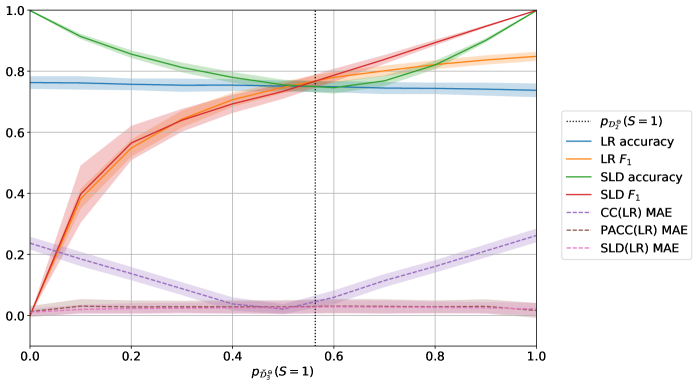
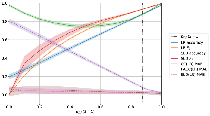
Figures 7 and 8 displays the quantification performance (MAE – dashed) and classification performance ($F_{1}$, accuracy – solid) of CC, SLD and PACC on the Adult dataset under protocols sample-prev-$\mathcal{D}_{2}$ and sample-prev-$\mathcal{D}_{3}$, respectively. As usual, we describe the results for LR-based learners and report their SVM-based duals in the appendix (Figures 12 and 13). To evaluate the quantification performance of each approach, we simply report their MAE in estimating the prevalence $p_{\mathcal{D}_{3}^{\ominus}}(S=1)$, $p_{\mathcal{D}_{3}^{\oplus}}(S=1)$ in either test subset, depending on the protocol at hand. To assess the performance of the sensitive attribute classifier $k$ underlying each quantifier, we proceed as follows. For CC and PACC, we simply run $k$ (LR) on either $\mathcal{D}_{3}^{\ominus}$ or $\mathcal{D}_{3}^{\oplus}$, reporting its accuracy and $F_{1}$ score in inferring the sensitive attribute of individual instances. The classification performance scores of the classifiers underlying CC and PACC are equivalent, so we omit the latter from Figures 7 and 8 for readability. For SLD, we take the novel posteriors obtained by applying the EM algorithm to either test subset, and use them for classification with a threshold of 0.5.

Clearly, SLD improves both the quantification and classification performance of the classifier $k$. In terms of quantification, its MAE is consistently below that of CC, and in terms of classification, it displays better $F_{1}$ and accuracy. However, under large prevalence shifts across the auxiliary set $\mathcal{D}_{2}$ and the test set $\mathcal{D}_{3}$, its classification performance becomes unreliable. In particular, under protocol sample-prev-$\mathcal{D}_{3}^{\ominus}$ (resp. sample-prev-$\mathcal{D}_{3}^{\oplus}$) in Figure 8(a) (resp. Figure 8(b)), for low values of the $x$ axis, i.e., when the true prevalence values $p_{\mathcal{D}_{3}^{\ominus}}(S=1)$ (resp. $p_{\mathcal{D}_{3}^{\oplus}}(S=1)$) becomes small, the SLD-based classifier starts acting as a trivial rejector with low recall, and hence low $F_{1}$ score. On the other hand, the quantification performance of SLD does not degrade in the same way, since its MAE is low and flat across the entire $x$ axis in Figures 8(a) and 8(b). This is a first hint of the fact that classification and quantification performance may be decoupled.

PACC is another method that significantly outperforms CC in estimating the prevalence of sensitive attributes in both test subsets $\mathcal{D}_{3}^{\ominus}$, $\mathcal{D}_{3}^{\oplus}$. Indeed, its MAE is well aligned with that of SLD, displaying low quantification error under all protocols (Figures 7–8). On the other hand, its classification performance is aligned with the accuracy and $F_{1}$ score of CC, which is unsatisfactory and can even become worse than random. This fact shows that it is possible to build models which yield good prevalence estimates for the sensitive attribute within a sample, without providing reliable demographic estimates for single instances. Indeed, quantification methods of type aggregative (that is, based on the output of a classifier – like all methods we use in this study) are suited to repair the initial prevalence estimate (computed by classifying and counting) without precise knowledge of which specific data points have been misclassified. In the context of models to measure fairness under unawareness of sensitive attributes, we highlight this as a positive result, decoupling a desirable ability to estimate group-level disparities from the potential for undesirable misuse at the individual level.

5.10 Ablation Study

5.10.1 Motivation and Setup

In the previous sections, we tested six approaches to estimate demographic disparity. For each approach, we used multiple quantifiers for the sensitive attribute $S$, namely one for each class in the codomain of the classifier $h$, as described in Step 3 of the method for quantification-based estimate of demographic disparity. In the binary setting adopted in this work, where $\mathcal{Y}=\{\ominus,\oplus\}$, we trained two quantifiers. A quantifier was trained on the set of positively-classified instances of the auxiliary set $\mathcal{D}_{2}^{\oplus}=\{(\mathbf{x}_{i},s_{i})\in\mathcal{D}_{2}\;|\;h(\mathbf{x})=\oplus\}$ and deployed to quantify the prevalence of sensitive instances (such that $S=s$) within the test subset $\mathcal{D}_{3}^{\oplus}$. The remaining quantifier was trained on $\mathcal{D}_{2}^{\ominus}$ and deployed on $\mathcal{D}_{3}^{\ominus}$.

Training and maintaining multiple quantifiers is more expensive and cumbersome than having a single one. Firstly, quantifiers that depend on the classification outcome $\hat{y}=h(\mathbf{x})$ require retraining every time $h$ is modified, e.g., due to a model update being rolled out. Second, the maintenance cost is multiplied by the number of classes $|\mathcal{Y}|$ that are possible for the outcome variable. To ensure that these downsides are compensated by performance improvements, we perform an ablation study and evaluate the performance of different estimators of demographic disparity supported by a single quantifier.

In this section we concentrate on three estimation approaches, namely PCC, SLD, and PACC. SLD and PACC are among the best overall performers, displaying low bias or variance across all protocols. PCC shows great performance in situations where its posteriors are well-calibrated on $\mathcal{D}_{3}$. We compare their performance in two settings. In the first setting, adopted so far, two separate quantifiers $q_{\ominus}$ and $q_{\oplus}$ are trained on $\mathcal{D}_{2}^{\ominus}$, $\mathcal{D}_{2}^{\oplus}$ and deployed on $\mathcal{D}_{3}^{\ominus}$, $\mathcal{D}_{3}^{\oplus}$, respectively. In the second setting, we train a single quantifier $q$ on $\mathcal{D}_{2}$ and deploy it separately on $\mathcal{D}_{3}^{\ominus}$ and $\mathcal{D}_{3}^{\oplus}$ to estimate $\hat{\delta_{h}^{S}}$ using Equations (14) and (15), specialized so that $q_{\ominus}$ and $q_{\oplus}$ are the same quantifier.

5.10.2 Results

(a) Protocol sample-prev-$\mathcal{D}_{2}^{\ominus}$

(b) Protocol sample-prev-$\mathcal{D}_{3}^{\ominus}$

Figure 9: Ablation study on the Adult dataset. Distribution of the estimation error ($y$ axis) for CC, PACC, SLD, and their single-quantifier counterparts, as $\Pr(S=1|\hat{Y}=\ominus)$ vary in $\mathcal{D}_{2}$, plot (a), and $\mathcal{D}_{3}$, plot (b).

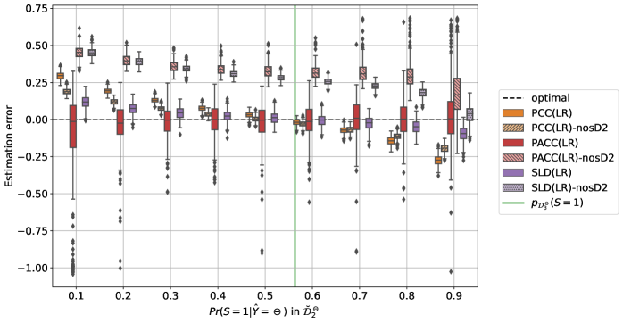
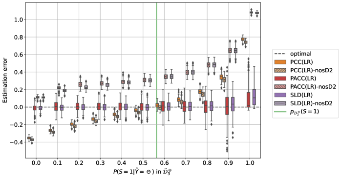
Figure 9 summarizes results for the Adult dataset under two protocols that are representative of the overall trends, namely sample-prev-$\mathcal{D}_{2}$ (Figure 9(a)) and sample-prev-$\mathcal{D}_{3}$ (Figure 9(b)). The $y$ axis depicts the estimation error of PCC, SLD, PACC, and their single-quantifier counterparts, denoted by the suffix “nosD2” to indicate that the auxiliary set $\mathcal{D}_{2}$ is not split into $\mathcal{D}_{2}^{\ominus}$, $\mathcal{D}_{2}^{\oplus}$ during training. The $x$ axis depicts the quantity of interest varied under each protocol.

Interestingly, PCC appears to be rather insensitive to the ablation study, so that the estimation errors of PCC and PCC-nosD2 are well-aligned. PCC-nosD2 performs slightly better under the protocol sample-prev-$\mathcal{D}_{2}$, where the auxiliary set is small, and splitting it to learn separate quantifiers may result in poor performance. The opposite is true for PACC-nosD2, showing a clear decline in performance in the single-quantifier setting. This is due to the fact that the estimates of $\mathrm{tpr}$ (and $\mathrm{fpr}$) in $\mathcal{D}_{3}^{\oplus}$ and $\mathcal{D}_{3}^{\ominus}$ for the adjustment (Equation 9) are more precise when issued by dedicated estimators rather than a single one computed without splitting $\mathcal{D}_{2}$. SLD-nosD2 also shows a sizeable performance decay.

Under all protocols, the performance of SLD and PACC is compromised in the absence of class-specific quantifiers $q_{\ominus}$ and $q_{\oplus}$. If a single quantifier is trained on the full auxiliary set $\mathcal{D}_{2}$, the corrections brought about by SLD and PACC can end up worsening, rather than improving, the prevalence estimates of vanilla CC. PCC is less sensitive to the ablation, showing small performance differences in both directions under the single quantifier setting. In general, it seems beneficial to partition the auxiliary set into subsets $\mathcal{D}_{2}^{\ominus}$ and $\mathcal{D}_{2}^{\oplus}$ according to the method in Section 4.2.

6 Summary and Takeaway Message

Overall, our work shows that quantification approaches are suited to measure demographic parity under unawareness of sensitive attributes if a small auxiliary dataset, containing sensitive and non-sensitive attributes, is available. This is a common setting in real-world scenarios, where such datasets may originate from targeted efforts or voluntary disclosure. Despite an inevitable selection bias, these datasets still represent a valuable asset for fairness audits, if coupled with robust estimation approaches. Indeed, several quantification methods tested in this work provide precise estimates of demographic disparity despite the distribution shift across training and testing caused by selection bias, and other distribution shifts that arise in the context of human processes. This is an important improvement over CC and PCC, previously studied in the algorithmic fairness literature as the threshold estimator and weighted estimator (Chen et al., 2019). SLD strikes the best balance in performance across all protocols; we suggest its adoption, especially when the distribution shift between development and deployment conditions has not been carefully characterized. Moreover, while the development of proxy methods typically comes with a potential for misuse on individuals (e.g., profiling), quantification approaches demonstrate the potential to circumvent this issue. More in detail, from the above experimental section, we summarize the following trends concerning different approaches to measure demographic parity under unawareness.

Fairness under unawareness can be measured using quantification, for both vanilla and fairness-aware classifiers. Group fairness under unawareness can be cast as a prevalence estimation problem and effectively solved by methods of proven consistency from the quantification literature. We demonstrate several estimators that outperform the previously proposed methods (Chen et al., 2019), corresponding to CC and PCC, i.e., two weak baselines in the quantification literature.

CC is suboptimal. Naïve Classify-and-Count represents the default approach for practitioners unaware of quantification. Ad hoc quantification methods outperform CC in most combinations of 5 protocols, 3 datasets, and 2 underlying learners.

PCC suffers under distribution shift. As long as the underlying posteriors are well-calibrated, PCC is a strong performer. However, when its training set and test set have different prevalence values for the sensitive attribute $S$, a common situation in practice, PCC displays a systematic estimation bias, which increases sharply with the prior probability shift between training and test.

HDy, ACC and PACC deteriorate in the small data regime. These methods require splitting their training set (that is, the auxiliary set $\mathcal{D}_{2}$), so their performance drops faster when its cardinality is small. PACC and ACC display good median performance but a large variance; the former method always outperforms the latter.

SLD strikes a good balance. This method was shown to be the best performer under (the inevitable) distribution shift between the auxiliary set $\mathcal{D}_{2}$ and the test set $\mathcal{D}_{3}$, with a moderate performance decrease when $|\mathcal{D}_{2}|$ becomes small. However, in situations where it is not possible to maintain separate quantifiers for positively and negatively predicted instances, its performance may drop substantially.

Decoupling is possible. Methods such as SLD and PACC fare much better than CC in estimating group-level quantities (such as demographic parity), while if misused for individual classification of sensitive attributes, the improvement is minor (SLD) or zero (PACC).

7 Conclusion

Measuring the differential impact of models on groups of individuals is important to understand their effects in the real world and their tendency to encode and reinforce divisions and privilege across sensitive attributes. Unfortunately, in practice, demographic attributes are often not available. In this work, we have taken the perspective of responsible practitioners, interested in internal fairness audits of production models. We have proposed a novel approach to measure group fairness under unawareness of sensitive attributes, utilizing methods from the quantification literature. These methods are specifically designed for group-level prevalence estimation rather than individual-level classification. Since practitioners who try to measure fairness under unawareness are precisely interested in prevalence estimates of sensitive attributes (Proposition 1), it is useful for the fairness and quantification communities to exchange lessons.

We have studied the problem of estimating a classifier’s fairness under unawareness of sensitive attributes, with access to a disjoint auxiliary set of data for which demographic information is available. We have shown how this can be cast as a quantification problem, and solved with established approaches of proven consistency. We have conducted a detailed empirical evaluation of different methods and their properties focused on demographic parity. Drawing from the algorithmic fairness literature, we have identified five important factors for this problem, associating each of them with a formal evaluation protocol. We have tested several quantification-based approaches, which, under realistic assumptions for an internal fairness audit, outperform previously proposed estimators in the fairness literature. We have discussed their benefits and limitations, including the unbiasedness guarantees of some methods, and the potential for misuse at an individual level.

Future work may require a deeper study of the relation between classification and quantification performance and the extent to which these two objectives can be decoupled. It would be interesting to explicitly target decoupling through learners aimed at maximizing quantification performance subject to a low classification performance constraint. Ideally, decoupling should provide precise privacy guarantees to individuals while allowing for precise group-level estimates. Another important avenue for future work is the study of confidence intervals for fairness estimates provided by quantification methods. A reliable indication of confidence for estimates of group fairness may be invaluable for a practitioner arguing for resources and attention to the disparate effects of a model on different populations. Finally, the estimators presented in this work may be plugged into optimization procedures aimed at improving, rather than measuring, algorithmic fairness. Mixed loss functions, jointly optimizing accuracy and fairness can be optimized, even under unawareness of sensitive attributes, with our methods providing fairness estimates at each iteration. It will be interesting to evaluate fairness estimators in this broader context and extend them, e.g., to ranking problems and counterfactual settings.

Acknowledgments

The work by Alessandro Fabris was supported by MIUR (Italian Ministry for University and Research) under the “Departments of Excellence” initiative (Law 232/2016). The work by Andrea Esuli, Alejandro Moreo, and Fabrizio Sebastiani has been supported by the SoBigData++ project, funded by the European Commission (Grant 871042) under the H2020 Programme INFRAIA-2019-1, by the AI4Media project, funded by the European Commission (Grant 951911) under the H2020 Programme ICT-48-2020, and by the SoBigData.it, FAIR and ITSERR projects funded by the Italian Ministry of University and Research under the NextGenerationEU program. These authors’ opinions do not necessarily reflect those of the funding agencies.

A The SLD Method

SLD (Saerens et al., 2002) produces prevalence estimates $\hat{p}_{\sigma}^{\mathrm{SLD}}(s)$ iteratively, using EM algorithms. In detail, given two sets, $L$ and $U$, where the former represents the labelled one (training set) and the latter represents the unlabelled one (test set). The method iterates until convergence (i.e., the difference between the prevalence estimated across two consecutive iterations is less than a tolerance factor $\epsilon$ –we use $\epsilon=1e-4$) or until a maximum number of iterations is reached. The pseudocode describing SLD is as follows:

Input : Class prevalence values $p_{L}(s)$ on $L$;

Posterior probabilities $\pi_{s}(\mathbf{x}_{i})$, for all $\mathbf{x}_{i}\in U$;

Output : Estimates $\hat{p}_{U}(s)$ of class prevalence values on $U$;

/* Initialisation */

$t\leftarrow 0$;

for $s\in S$ do

       $\hat{p}^{(t)}_{U}(s)\leftarrow p_{L}(s)$;

       for $\mathbf{x}_{i}\in U$ do

             $\Pr^{(t)}(s|\textbf{x}_{i})\leftarrow\pi_{s}(\mathbf{x}_{i})$;

       end for

      

end for

/* Main Iteration Cycle */

while stopping condition = false do

       $t\leftarrow t+1$;

       for $s\in S$ do

             for $\mathbf{x}_{i}\in U$ do

                   $\Pr^{(t)}(s|\textbf{x}_{i})\leftarrow\displaystyle\frac{\displaystyle\frac{\hat{p}^{(t-1)}_{U}(s)}{\hat{p}^{(0)}_{U}(s)}\cdot\Pr^{(0)}(s|\textbf{x}_{i})}{\displaystyle\sum_{s\in S}\displaystyle\frac{\hat{p}^{(t-1)}_{U}(s)}{\hat{p}^{(0)}_{U}(s)}\cdot\Pr^{(0)}(s|\textbf{x}_{i})}$

             end for

            $\hat{p}^{(t)}_{U}(s)\leftarrow\displaystyle\frac{1}{|U|}\displaystyle\sum_{\textbf{x}_{i}\in U}\Pr^{(t)}(s|\textbf{x}_{i})$

       end for

      

end while

/* Generate output */

for $s\in S$ do

      $\hat{p}_{U}^{\mathrm{SLD}}(s)\leftarrow\hat{p}^{(t)}_{U}(s)$

end for

Pseudocode 2 The SLD algorithm (Saerens et al., 2002).

B The HDy Method

HDy (González-Castro et al., 2013) measures the divergence between two distributions of posterior probabilities (i.e., as returned by a calibrated classifier) $v$ and $u$ in terms of the Hellinger Distance (HD), defined as

$$\mathrm{HD}(v,u)=\sqrt{\int\left(\sqrt{v(x)}-\sqrt{u(x)}\right)^{2}dx}$$

The HD between two continuous distributions $v$ and $u$ is typically approximated by discretizing $v$ and $u$ across bins and then integrating

$$\hat{\mathrm{HD}}(V,U)=\sqrt{\sum_{i=1}^{b}\left(\sqrt{\frac{|V_{i}|}{|V|}}-\sqrt{\frac{|U_{i}|}{|U|}}\right)^{2}}$$

with $V$ and $U$ the discrete distributions, $b$ the number of bins and $V_{i}$, $U_{i}$ representing the frequency in the $i$th bin for each distribution, respectively.

The method seeks the $\alpha$ parameter that yields the smallest distance between the validation distribution $V$ (typically, a held-out split of the training set that has not been used to train the classifier) and the unlabelled distribution $U$, i.e.,

$$\alpha^{*}=\arg\min_{\alpha\in[0,1]}\hat{\mathrm{HD}}(V^{\alpha},U)$$

where $V^{\alpha}$ is the mixture of the positive distribution ($V^{S=1}$) and the negative distribution ($V^{S=0}$) defined by

$$V^{\alpha}(x)=(1-\alpha)\cdot V^{S=0}(x)+\alpha\cdot V^{S=1}(x)$$

HDy returns $\alpha^{*}$ as the sought positive class prevalence

$$\hat{p}_{\sigma}^{\mathrm{HDy}}(1)=\alpha^{*}$$

Since the number of bins $b$ could have a significant impact on the calculation, one typically returns the median of the distribution of the best $\alpha$’s found for a range of $b$’s (in our case, we explore $b\in[10,20,30,\ldots,110]$).

C Proof of Proposition 2

We show that Equation (2) and Equation (15) are equivalent when the latter is instantiated by prevalence estimates given by PCC:

$$\hat{\mu}^{\mathrm{PCC}}(s) =\hat{p}_{\mathcal{D}_{3}^{\oplus}}^{\mathrm{PCC}}(s)\frac{p_{\mathcal{D}_{3}}(\oplus)}{\hat{p}_{\mathcal{D}_{3}^{\oplus}}^{\mathrm{PCC}}(s)p_{\mathcal{D}_{3}}(\oplus)+\hat{p}_{\mathcal{D}_{3}^{\ominus}}^{\mathrm{PCC}}(s)p_{\mathcal{D}_{3}}(\ominus)}$$

The terms in the denominator can be written as

$$\hat{p}_{\mathcal{D}_{3}^{\oplus}}^{\mathrm{PCC}}(s) =\frac{\sum_{\mathbf{x}_{i}\in\mathcal{D}_{3}^{\oplus}}\pi_{s}(\mathbf{x}_{i})}{|\mathcal{D}_{3}^{\oplus}|}$$

$$=\frac{\sum_{\mathbf{x}_{i}}\pi_{s}(\mathbf{x}_{i})h_{\oplus}(\mathbf{x}_{i})}{\sum_{\mathbf{x}_{i}}h_{\oplus}(\mathbf{x}_{i})}$$

$$\hat{p}_{\mathcal{D}_{3}^{\ominus}}^{\mathrm{PCC}}(s)=\frac{\sum_{\mathbf{x}_{i}}\pi_{s}(\mathbf{x}_{i})(1-h_{\oplus}(\mathbf{x}_{i}))}{\sum_{\mathbf{x}_{i}}(1-h_{\oplus}(\mathbf{x}_{i}))}$$

$$p_{\mathcal{D}_{3}}(\oplus)=\frac{\sum_{\mathbf{x}_{i}}h_{\oplus}(\mathbf{x}_{i})}{|\mathcal{D}_{3}|}$$

$$p_{\mathcal{D}_{3}}(\ominus)=\frac{\sum_{\mathbf{x}_{i}}(1-h_{\oplus}(\mathbf{x}_{i}))}{|\mathcal{D}_{3}|}$$

Plugging them into the denominator yields

$$\hat{\mu}^{\mathrm{PCC}}(s) =\hat{p}_{\mathcal{D}_{3}^{\oplus}}^{\mathrm{PCC}}(s)\frac{p_{\mathcal{D}_{3}}(\oplus)}{\frac{\sum_{\mathbf{x}_{i}}\pi_{s}(\mathbf{x}_{i})}{|\mathcal{D}_{3}|}}$$

$$=\frac{\sum_{\mathbf{x}_{i}}\pi_{s}(\mathbf{x}_{i})h_{\oplus}(\mathbf{x}_{i})}{\sum_{\mathbf{x}_{i}}h_{\oplus}(\mathbf{x}_{i})}\cdot\frac{\sum_{\mathbf{x}_{i}}h_{\oplus}(\mathbf{x}_{i})}{|\mathcal{D}_{3}|}\cdot\frac{|\mathcal{D}_{3}|}{\sum_{\mathbf{x}_{i}}\pi_{s}(\mathbf{x}_{i})}$$

$$=\hat{\mu}^{\mathrm{WE}}(s)$$

The equivalence between CC and TE is straightforward. ∎

D SVM-based Quantification

In this appendix we report the results of experiments, analogous to the ones in Sections 5.6-5.9, where quantifiers are wrapped around an SVM classifier rather than an LR classifier. The experimental protocols are summarized in Tables 9-13. The ablation study is depicted in Figures 10 and 11. Experiments on decoupling the quantification performance of a model from its classification performance are reported in Figures 12 and 13.

Table 9: Results obtained in the experiments run according to protocol sample-prev-$\mathcal{D}_{3}$ with the SVM-based classifier.

		$\downarrow$ MAE	$\downarrow$ MSE	$\uparrow$ $P(\mathrm{AE}<0.1)$	$\uparrow$ $P(\mathrm{AE}<0.2)$
Adult	CC(SVM)	0.410${}^{\phantom{{\ddagger}}}\pm 0.323$	0.273${}^{\phantom{{\ddagger}}}\pm 0.341$	0.193	0.365
	PCC(SVM)	0.308${}^{\phantom{{\ddagger}}}\pm 0.244$	0.154${}^{\phantom{{\ddagger}}}\pm 0.210$	0.230	0.412
	ACC(SVM)	0.107${}^{\phantom{{\ddagger}}}\pm 0.105$	0.022${}^{\phantom{{\ddagger}}}\pm 0.053$	0.606	0.857
	PACC(SVM)	0.059${}^{\phantom{{\ddagger}}}\pm 0.057$	0.007${}^{\phantom{{\ddagger}}}\pm 0.016$	0.824	0.971
	SLD(SVM)	0.056${}^{\phantom{{\ddagger}}}\pm 0.050$	0.006${}^{\phantom{{\ddagger}}}\pm 0.011$	0.836	0.983
	HDy(SVM)	0.104${}^{\phantom{{\ddagger}}}\pm 0.078$	0.017${}^{\phantom{{\ddagger}}}\pm 0.028$	0.546	0.895
	MLPE	0.397${}^{\phantom{{\ddagger}}}\pm 0.298$	0.246${}^{\phantom{{\ddagger}}}\pm 0.316$	0.162	0.294
COMPAS	CC(SVM)	0.543${}^{\phantom{{\ddagger}}}\pm 0.370$	0.432${}^{\phantom{{\ddagger}}}\pm 0.474$	0.115	0.235
	PCC(SVM)	0.339${}^{\phantom{{\ddagger}}}\pm 0.243$	0.174${}^{\phantom{{\ddagger}}}\pm 0.216$	0.179	0.343
	ACC(SVM)	0.497${}^{\phantom{{\ddagger}}}\pm 0.346$	0.367${}^{\phantom{{\ddagger}}}\pm 0.448$	0.127	0.224
	PACC(SVM)	0.269${}^{\phantom{{\ddagger}}}\pm 0.207$	0.115${}^{\phantom{{\ddagger}}}\pm 0.165$	0.250	0.445
	SLD(SVM)	0.227${}^{\phantom{{\ddagger}}}\pm 0.202$	0.092${}^{\phantom{{\ddagger}}}\pm 0.154$	0.335	0.566
	HDy(SVM)	0.265${}^{\phantom{{\ddagger}}}\pm 0.204$	0.112${}^{\phantom{{\ddagger}}}\pm 0.162$	0.238	0.459
	MLPE	0.349${}^{\phantom{{\ddagger}}}\pm 0.249$	0.184${}^{\phantom{{\ddagger}}}\pm 0.227$	0.175	0.332
CreditCard	CC(SVM)	0.346${}^{\phantom{{\ddagger}}}\pm 0.241$	0.178${}^{\phantom{{\ddagger}}}\pm 0.213$	0.171	0.335
	PCC(SVM)	0.329${}^{\phantom{{\ddagger}}}\pm 0.215$	0.155${}^{\phantom{{\ddagger}}}\pm 0.161$	0.173	0.335
	ACC(SVM)	0.358${}^{\phantom{{\ddagger}}}\pm 0.270$	0.201${}^{\phantom{{\ddagger}}}\pm 0.276$	0.175	0.348
	PACC(SVM)	0.267${}^{\phantom{{\ddagger}}}\pm 0.215$	0.118${}^{\phantom{{\ddagger}}}\pm 0.180$	0.252	0.473
	SLD(SVM)	0.243${}^{{\ddagger}}\pm 0.191$	0.096${}^{{\dagger}}\pm 0.143$	0.268	0.496
	HDy(SVM)	0.237${}^{\phantom{{\ddagger}}}\pm 0.186$	0.090${}^{\phantom{{\ddagger}}}\pm 0.137$	0.271	0.507
	MLPE	0.334${}^{\phantom{{\ddagger}}}\pm 0.218$	0.159${}^{\phantom{{\ddagger}}}\pm 0.165$	0.172	0.330

Table 10: Results obtained in the experiments run according to protocol sample-prev-$\mathcal{D}_{2}$ with the SVM-based classifier.

		$\downarrow$ MAE	$\downarrow$ MSE	$\uparrow$ $P(\mathrm{AE}<0.1)$	$\uparrow$ $P(\mathrm{AE}<0.2)$
Adult	CC(SVM)	0.217${}^{\phantom{{\ddagger}}}\pm 0.168$	0.075${}^{\phantom{{\ddagger}}}\pm 0.106$	0.286	0.554
	PCC(SVM)	0.242${}^{\phantom{{\ddagger}}}\pm 0.190$	0.095${}^{\phantom{{\ddagger}}}\pm 0.129$	0.303	0.507
	ACC(SVM)	0.150${}^{\phantom{{\ddagger}}}\pm 0.169$	0.051${}^{\phantom{{\ddagger}}}\pm 0.147$	0.458	0.799
	PACC(SVM)	0.111${}^{\phantom{{\ddagger}}}\pm 0.114$	0.025${}^{\phantom{{\ddagger}}}\pm 0.085$	0.555	0.888
	SLD(SVM)	0.095${}^{\phantom{{\ddagger}}}\pm 0.100$	0.019${}^{\phantom{{\ddagger}}}\pm 0.067$	0.634	0.929
	HDy(SVM)	0.182${}^{\phantom{{\ddagger}}}\pm 0.151$	0.056${}^{\phantom{{\ddagger}}}\pm 0.084$	0.381	0.634
	MLPE	0.295${}^{\phantom{{\ddagger}}}\pm 0.218$	0.134${}^{\phantom{{\ddagger}}}\pm 0.165$	0.240	0.415
COMPAS	CC(SVM)	0.506${}^{\phantom{{\ddagger}}}\pm 0.255$	0.321${}^{\phantom{{\ddagger}}}\pm 0.267$	0.036	0.116
	PCC(SVM)	0.266${}^{\phantom{{\ddagger}}}\pm 0.187$	0.106${}^{{\ddagger}}\pm 0.128$	0.226	0.430
	ACC(SVM)	0.479${}^{\phantom{{\ddagger}}}\pm 0.276$	0.306${}^{\phantom{{\ddagger}}}\pm 0.305$	0.076	0.175
	PACC(SVM)	0.356${}^{\phantom{{\ddagger}}}\pm 0.260$	0.194${}^{\phantom{{\ddagger}}}\pm 0.261$	0.167	0.324
	SLD(SVM)	0.297${}^{\phantom{{\ddagger}}}\pm 0.244$	0.148${}^{\phantom{{\ddagger}}}\pm 0.228$	0.231	0.424
	HDy(SVM)	0.255${}^{\phantom{{\ddagger}}}\pm 0.192$	0.102${}^{\phantom{{\ddagger}}}\pm 0.141$	0.240	0.479
	MLPE	0.275${}^{\phantom{{\ddagger}}}\pm 0.192$	0.112${}^{\phantom{{\ddagger}}}\pm 0.134$	0.220	0.410
CreditCard	CC(SVM)	0.428${}^{\phantom{{\ddagger}}}\pm 0.253$	0.247${}^{\phantom{{\ddagger}}}\pm 0.237$	0.106	0.229
	PCC(SVM)	0.209${}^{\phantom{{\ddagger}}}\pm 0.142$	0.064${}^{\phantom{{\ddagger}}}\pm 0.076$	0.285	0.537
	ACC(SVM)	0.531${}^{\phantom{{\ddagger}}}\pm 0.316$	0.382${}^{\phantom{{\ddagger}}}\pm 0.352$	0.090	0.164
	PACC(SVM)	0.542${}^{\phantom{{\ddagger}}}\pm 0.313$	0.391${}^{\phantom{{\ddagger}}}\pm 0.352$	0.078	0.145
	SLD(SVM)	0.445${}^{\phantom{{\ddagger}}}\pm 0.284$	0.279${}^{\phantom{{\ddagger}}}\pm 0.288$	0.118	0.237
	HDy(SVM)	0.246${}^{\phantom{{\ddagger}}}\pm 0.193$	0.098${}^{\phantom{{\ddagger}}}\pm 0.150$	0.256	0.487
	MLPE	0.210${}^{{\ddagger}}\pm 0.143$	0.065${}^{{\ddagger}}\pm 0.077$	0.287	0.530

Table 11: Results obtained in the experiments run according to protocol sample-size-$\mathcal{D}_{2}$ with the SVM-based classifier

		$\downarrow$ MAE	$\downarrow$ MSE	$\uparrow$ $P(\mathrm{AE}<0.1)$	$\uparrow$ $P(\mathrm{AE}<0.2)$
Adult	CC(SVM)	0.131${}^{\phantom{{\ddagger}}}\pm 0.028$	0.018${}^{\phantom{{\ddagger}}}\pm 0.007$	0.133	1.000
	PCC(SVM)	0.012${}^{\phantom{{\ddagger}}}\pm 0.011$	0.000${}^{\phantom{{\ddagger}}}\pm 0.000$	1.000	1.000
	ACC(SVM)	0.081${}^{\phantom{{\ddagger}}}\pm 0.107$	0.018${}^{\phantom{{\ddagger}}}\pm 0.076$	0.759	0.935
	PACC(SVM)	0.051${}^{\phantom{{\ddagger}}}\pm 0.066$	0.007${}^{\phantom{{\ddagger}}}\pm 0.036$	0.873	0.977
	SLD(SVM)	0.043${}^{\phantom{{\ddagger}}}\pm 0.062$	0.006${}^{\phantom{{\ddagger}}}\pm 0.030$	0.907	0.971
	HDy(SVM)	0.045${}^{\phantom{{\ddagger}}}\pm 0.034$	0.003${}^{\phantom{{\ddagger}}}\pm 0.005$	0.918	0.999
	MLPE	0.013${}^{{\ddagger}}\pm 0.011$	0.000${}^{{\ddagger}}\pm 0.001$	1.000	1.000
COMPAS	CC(SVM)	0.355${}^{\phantom{{\ddagger}}}\pm 0.044$	0.128${}^{\phantom{{\ddagger}}}\pm 0.031$	0.000	0.003
	PCC(SVM)	0.029${}^{\phantom{{\ddagger}}}\pm 0.019$	0.001${}^{\phantom{{\ddagger}}}\pm 0.001$	0.999	1.000
	ACC(SVM)	0.389${}^{\phantom{{\ddagger}}}\pm 0.212$	0.196${}^{\phantom{{\ddagger}}}\pm 0.212$	0.090	0.171
	PACC(SVM)	0.284${}^{\phantom{{\ddagger}}}\pm 0.231$	0.134${}^{\phantom{{\ddagger}}}\pm 0.210$	0.233	0.444
	SLD(SVM)	0.228${}^{\phantom{{\ddagger}}}\pm 0.199$	0.092${}^{\phantom{{\ddagger}}}\pm 0.158$	0.305	0.555
	HDy(SVM)	0.130${}^{\phantom{{\ddagger}}}\pm 0.102$	0.027${}^{\phantom{{\ddagger}}}\pm 0.041$	0.461	0.778
	MLPE	0.029${}^{{\ddagger}}\pm 0.021$	0.001${}^{{\ddagger}}\pm 0.002$	0.999	1.000
CreditCard	CC(SVM)	0.189${}^{\phantom{{\ddagger}}}\pm 0.079$	0.042${}^{\phantom{{\ddagger}}}\pm 0.032$	0.132	0.552
	PCC(SVM)	0.016${}^{\phantom{{\ddagger}}}\pm 0.013$	0.000${}^{\phantom{{\ddagger}}}\pm 0.001$	1.000	1.000
	ACC(SVM)	0.358${}^{\phantom{{\ddagger}}}\pm 0.269$	0.201${}^{\phantom{{\ddagger}}}\pm 0.267$	0.181	0.328
	PACC(SVM)	0.322${}^{\phantom{{\ddagger}}}\pm 0.257$	0.169${}^{\phantom{{\ddagger}}}\pm 0.248$	0.213	0.385
	SLD(SVM)	0.243${}^{\phantom{{\ddagger}}}\pm 0.192$	0.096${}^{\phantom{{\ddagger}}}\pm 0.142$	0.284	0.497
	HDy(SVM)	0.105${}^{\phantom{{\ddagger}}}\pm 0.096$	0.020${}^{\phantom{{\ddagger}}}\pm 0.051$	0.583	0.876
	MLPE	0.017${}^{{\ddagger}}\pm 0.013$	0.000${}^{{\ddagger}}\pm 0.001$	1.000	1.000

Table 12: Results obtained in the experiments run according to protocol sample-prev-$\mathcal{D}_{1}$ with the SVM-based classifier.

		$\downarrow$ MAE	$\downarrow$ MSE	$\uparrow$ $P(\mathrm{AE}<0.1)$	$\uparrow$ $P(\mathrm{AE}<0.2)$
Adult	CC(SVM)	0.126${}^{\phantom{{\ddagger}}}\pm 0.047$	0.018${}^{\phantom{{\ddagger}}}\pm 0.011$	0.268	0.959
	PCC(SVM)	0.007${}^{\phantom{{\ddagger}}}\pm 0.005$	0.000${}^{\phantom{{\ddagger}}}\pm 0.000$	1.000	1.000
	ACC(SVM)	0.032${}^{\phantom{{\ddagger}}}\pm 0.032$	0.002${}^{\phantom{{\ddagger}}}\pm 0.014$	0.968	0.998
	PACC(SVM)	0.018${}^{\phantom{{\ddagger}}}\pm 0.014$	0.001${}^{\phantom{{\ddagger}}}\pm 0.001$	1.000	1.000
	SLD(SVM)	0.013${}^{\phantom{{\ddagger}}}\pm 0.010$	0.000${}^{\phantom{{\ddagger}}}\pm 0.000$	1.000	1.000
	HDy(SVM)	0.022${}^{\phantom{{\ddagger}}}\pm 0.016$	0.001${}^{\phantom{{\ddagger}}}\pm 0.001$	1.000	1.000
	MLPE	0.008${}^{\phantom{{\ddagger}}}\pm 0.006$	0.000${}^{\phantom{{\ddagger}}}\pm 0.000$	1.000	1.000
COMPAS	CC(SVM)	0.334${}^{\phantom{{\ddagger}}}\pm 0.087$	0.119${}^{\phantom{{\ddagger}}}\pm 0.055$	0.018	0.063
	PCC(SVM)	0.026${}^{\phantom{{\ddagger}}}\pm 0.018$	0.001${}^{\phantom{{\ddagger}}}\pm 0.001$	1.000	1.000
	ACC(SVM)	0.349${}^{\phantom{{\ddagger}}}\pm 0.196$	0.160${}^{\phantom{{\ddagger}}}\pm 0.174$	0.123	0.221
	PACC(SVM)	0.208${}^{\phantom{{\ddagger}}}\pm 0.179$	0.075${}^{\phantom{{\ddagger}}}\pm 0.134$	0.332	0.578
	SLD(SVM)	0.170${}^{\phantom{{\ddagger}}}\pm 0.166$	0.057${}^{\phantom{{\ddagger}}}\pm 0.117$	0.422	0.707
	HDy(SVM)	0.113${}^{\phantom{{\ddagger}}}\pm 0.089$	0.021${}^{\phantom{{\ddagger}}}\pm 0.031$	0.528	0.839
	MLPE	0.027${}^{{\ddagger}}\pm 0.019$	0.001${}^{{\ddagger}}\pm 0.001$	1.000	1.000
CreditCard	CC(SVM)	0.152${}^{\phantom{{\ddagger}}}\pm 0.100$	0.033${}^{\phantom{{\ddagger}}}\pm 0.038$	0.360	0.708
	PCC(SVM)	0.010${}^{\phantom{{\ddagger}}}\pm 0.007$	0.000${}^{\phantom{{\ddagger}}}\pm 0.000$	1.000	1.000
	ACC(SVM)	0.194${}^{\phantom{{\ddagger}}}\pm 0.160$	0.063${}^{\phantom{{\ddagger}}}\pm 0.104$	0.342	0.618
	PACC(SVM)	0.132${}^{\phantom{{\ddagger}}}\pm 0.108$	0.029${}^{\phantom{{\ddagger}}}\pm 0.046$	0.482	0.778
	SLD(SVM)	0.110${}^{\phantom{{\ddagger}}}\pm 0.091$	0.020${}^{\phantom{{\ddagger}}}\pm 0.032$	0.560	0.845
	HDy(SVM)	0.080${}^{\phantom{{\ddagger}}}\pm 0.061$	0.010${}^{\phantom{{\ddagger}}}\pm 0.014$	0.683	0.953
	MLPE	0.011${}^{{\dagger}}\pm 0.008$	0.000${}^{\phantom{{\ddagger}}}\pm 0.000$	1.000	1.000

Table 13: Results obtained in the experiments run according to protocol flip-prev-$\mathcal{D}_{1}$ with the SVM-based classifier.

		$\downarrow$ MAE	$\downarrow$ MSE	$\uparrow$ $P(\mathrm{AE}<0.1)$	$\uparrow$ $P(\mathrm{AE}<0.2)$
Adult	CC(SVM)	0.175${}^{\phantom{{\ddagger}}}\pm 0.085$	0.038${}^{\phantom{{\ddagger}}}\pm 0.028$	0.231	0.544
	PCC(SVM)	0.007${}^{\phantom{{\ddagger}}}\pm 0.006$	0.000${}^{\phantom{{\ddagger}}}\pm 0.000$	1.000	1.000
	ACC(SVM)	0.032${}^{\phantom{{\ddagger}}}\pm 0.028$	0.002${}^{\phantom{{\ddagger}}}\pm 0.004$	0.969	0.999
	PACC(SVM)	0.020${}^{\phantom{{\ddagger}}}\pm 0.015$	0.001${}^{\phantom{{\ddagger}}}\pm 0.001$	1.000	1.000
	SLD(SVM)	0.015${}^{\phantom{{\ddagger}}}\pm 0.012$	0.000${}^{\phantom{{\ddagger}}}\pm 0.001$	1.000	1.000
	HDy(SVM)	0.022${}^{\phantom{{\ddagger}}}\pm 0.018$	0.001${}^{\phantom{{\ddagger}}}\pm 0.001$	1.000	1.000
	MLPE	0.009${}^{\phantom{{\ddagger}}}\pm 0.006$	0.000${}^{\phantom{{\ddagger}}}\pm 0.000$	1.000	1.000
COMPAS	CC(SVM)	0.395${}^{\phantom{{\ddagger}}}\pm 0.113$	0.169${}^{\phantom{{\ddagger}}}\pm 0.083$	0.021	0.055
	PCC(SVM)	0.027${}^{\phantom{{\ddagger}}}\pm 0.019$	0.001${}^{\phantom{{\ddagger}}}\pm 0.001$	0.998	1.000
	ACC(SVM)	0.399${}^{\phantom{{\ddagger}}}\pm 0.204$	0.201${}^{\phantom{{\ddagger}}}\pm 0.193$	0.094	0.174
	PACC(SVM)	0.207${}^{\phantom{{\ddagger}}}\pm 0.176$	0.074${}^{\phantom{{\ddagger}}}\pm 0.131$	0.325	0.587
	SLD(SVM)	0.160${}^{\phantom{{\ddagger}}}\pm 0.146$	0.047${}^{\phantom{{\ddagger}}}\pm 0.095$	0.418	0.722
	HDy(SVM)	0.112${}^{\phantom{{\ddagger}}}\pm 0.084$	0.020${}^{\phantom{{\ddagger}}}\pm 0.028$	0.528	0.842
	MLPE	0.027${}^{{\ddagger}}\pm 0.019$	0.001${}^{{\ddagger}}\pm 0.001$	0.999	1.000
CreditCard	CC(SVM)	0.165${}^{\phantom{{\ddagger}}}\pm 0.105$	0.038${}^{\phantom{{\ddagger}}}\pm 0.039$	0.328	0.627
	PCC(SVM)	0.012${}^{{\ddagger}}\pm 0.009$	0.000${}^{{\ddagger}}\pm 0.000$	1.000	1.000
	ACC(SVM)	0.227${}^{\phantom{{\ddagger}}}\pm 0.186$	0.086${}^{\phantom{{\ddagger}}}\pm 0.130$	0.303	0.542
	PACC(SVM)	0.144${}^{\phantom{{\ddagger}}}\pm 0.120$	0.035${}^{\phantom{{\ddagger}}}\pm 0.059$	0.442	0.742
	SLD(SVM)	0.118${}^{\phantom{{\ddagger}}}\pm 0.095$	0.023${}^{\phantom{{\ddagger}}}\pm 0.036$	0.512	0.819
	HDy(SVM)	0.092${}^{\phantom{{\ddagger}}}\pm 0.070$	0.013${}^{\phantom{{\ddagger}}}\pm 0.019$	0.621	0.913
	MLPE	0.012${}^{\phantom{{\ddagger}}}\pm 0.009$	0.000${}^{\phantom{{\ddagger}}}\pm 0.000$	1.000	1.000

(a) Protocol sample-prev-$\mathcal{D}_{2}^{\ominus}$

(b) Protocol sample-prev-$\mathcal{D}_{2}^{\oplus}$

Figure 10: Results obtained in the ablation study on the Adult dataset with SVM-based quantification for protocol sample-prev-$\mathcal{D}_{2}$.

(a) Protocol sample-prev-$\mathcal{D}_{3}^{\ominus}$

(b) Protocol sample-prev-$\mathcal{D}_{3}^{\oplus}$

Figure 11: Results obtained in the ablation study on the Adult dataset with SVM-based quantification for protocol sample-prev-$\mathcal{D}_{3}$.

(a) Protocol sample-prev-$\mathcal{D}_{2}^{\ominus}$

(b) Protocol sample-prev-$\mathcal{D}_{2}^{\oplus}$

Figure 12: Performance of SVM-based methods CC, SLD and PACC on the Adult dataset when used for quantification (MAE – lower is better) and classification ($F_{1}$, accuracy – higher is better) under protocol sample-prev-$\mathcal{D}_{2}$. The classification performance of PACC is equivalent to that of CC (both equal to the performance of the underlying SVM), and we thus omit it for readability.

(a) Protocol sample-prev-$\mathcal{D}_{3}^{\ominus}$

(b) Protocol sample-prev-$\mathcal{D}_{3}^{\oplus}$

Figure 13: Performance of SVM-based methods CC, SLD and PACC on the Adult dataset when used for quantification (MAE – lower is better) and classification ($F_{1}$, accuracy – higher is better) under protocol sample-prev-$\mathcal{D}_{3}$. The classification performance of PACC is equivalent to that of CC (both equal to the performance of the underlying SVM), and we thus omit it for readability.

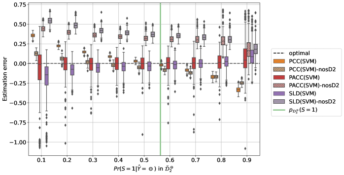
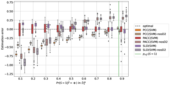
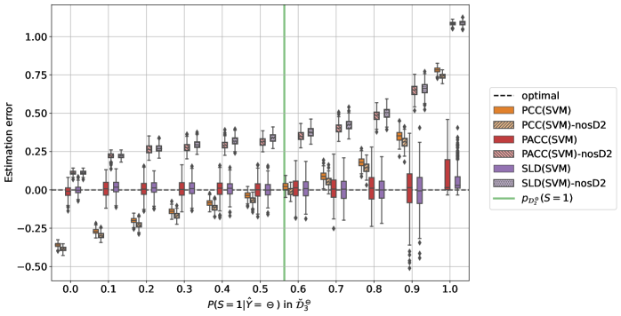
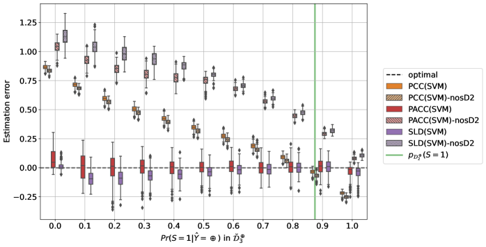
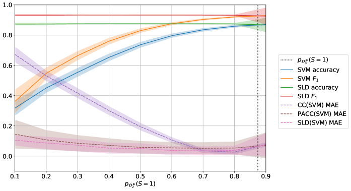
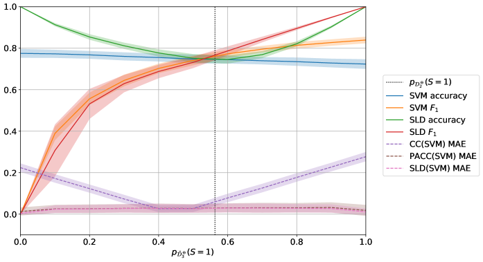
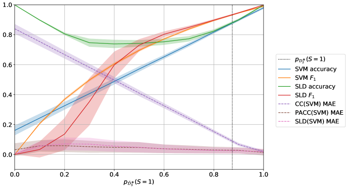
E Pseudocode

This section reports pseudocode for protocols sample-prev-$\mathcal{D}_{2}$ (Pseudocode 3), sample-size-$\mathcal{D}_{2}$ (Pseudocode 4), and sample-prev-$\mathcal{D}_{1}$ (Pseudocode 5).

Input :  • Dataset $\mathcal{D}$ ;

 • Classifier learner CLS;

 • Quantification method Q;

Output :  • MAE of the demographic disparity estimates ;

 • MSE of the demographic disparity estimates ;

1

2$E\leftarrow\emptyset$ ;

3for 5 random splits do

4       $\mathcal{D}_{A},\mathcal{D}_{B},\mathcal{D}_{C}\leftarrow\mathrm{split\_stratify}(\mathcal{D})$ ;

5      for $\mathcal{D}_{1},\mathcal{D}_{2},\mathcal{D}_{3}\in\mathrm{permutations}(\mathcal{D}_{A},\mathcal{D}_{B},\mathcal{D}_{C})$ do

6            

7            /* Learn a classifier $h:\mathcal{X}\rightarrow\mathcal{Y}$ */

8             $h\leftarrow$ CLS.fit($\mathcal{D}_{1}$) ;

9            $\mathcal{D}_{2}^{\ominus}\leftarrow\{(\mathbf{x}_{i},s_{i})\in\mathcal{D}_{2}\;|\;h(\mathbf{x}_{i})=\ominus\}$ ;

10            $\mathcal{D}_{2}^{\oplus}\leftarrow\{(\mathbf{x}_{i},s_{i})\in\mathcal{D}_{2}\;|\;h(\mathbf{x}_{i})=\oplus\}$ ;

11            for 10 repeats do

12                  

13                   for $p\in\{0.1,0.2,\ldots,0.9\}$ do

14                        

15                        /* Generate samples from $\mathcal{D}_{2}^{\ominus}$ at desired prevalence and size, and uniform samples from $\mathcal{D}_{2}^{\oplus}$ at desired size */

16                        

17                        $\breve{\mathcal{D}}_{2}^{\ominus}\sim\mathcal{D}_{2}^{\ominus}$ with $p_{\breve{\mathcal{D}}_{2}^{\ominus}}(s)=p$ and $|\breve{\mathcal{D}}_{2}^{\ominus}|=500$ ;

18                        $\breve{\mathcal{D}}_{2}^{\oplus}\sim\mathcal{D}_{2}^{\oplus}$ with $|\breve{\mathcal{D}}_{2}^{\oplus}|=500$ ;

19                        /* Learn quantifiers $q_{y}:2^{\mathcal{X}}\rightarrow[0,1]$ */

20                        

21                        $q_{\ominus}\leftarrow$ Q.fit($\breve{\mathcal{D}}_{2}^{\ominus})$ ;

22                        $q_{\oplus}\leftarrow$ Q.fit($\breve{\mathcal{D}}_{2}^{\oplus})$ ;

23                         /* Use quantifiers to estimate demographic prevalence */

24                         $\mathcal{D}_{3}^{\ominus}\leftarrow\{\mathbf{x}_{i}\in\mathcal{D}_{3}\;|\;h(\mathbf{x}_{i})=\ominus\}$ ;

25                        $\mathcal{D}_{3}^{\oplus}\leftarrow\{\mathbf{x}_{i}\in\mathcal{D}_{3}\;|\;h(\mathbf{x}_{i})=\oplus\}$ ;

26                        $\hat{p}^{q_{\ominus}}_{\mathcal{D}_{3}^{\ominus}}(s)\leftarrow q_{\ominus}(\mathcal{D}_{3}^{\ominus})$ ;

27                        $\hat{p}^{q_{\oplus}}_{\mathcal{D}_{3}^{\oplus}}(s)\leftarrow q_{\oplus}(\mathcal{D}_{3}^{\oplus})$ ;

28                        /* Compute the signed error of the demographic disparity estimate */

29                         $e\leftarrow$ compute error using $\hat{p}^{q_{\ominus}}_{\mathcal{D}_{3}^{\ominus}}(s)$, $\hat{p}^{q_{\oplus}}_{\mathcal{D}_{3}^{\oplus}}(s)$ and Equation 16

30                        $E\leftarrow E\cup\{e\}$

31                   end for

32                  

33             end for

34            

35       end for

36      

37 end for

38

39$\mathrm{mae}\leftarrow\mathrm{MAE}(E)$ ;

40$\mathrm{mse}\leftarrow\mathrm{MSE}(E)$ ;

41return $\mathrm{mae}$, $\mathrm{mse}$

Pseudocode 3 Protocol sample-prev-$\mathcal{D}_{2}$, shown for variations of prevalence values in class $y=\ominus$.

Input :  • Dataset $\mathcal{D}$ ;

 • Classifier learner CLS;

 • Quantification method Q;

Output :  • MAE of the demographic disparity estimates ;

 • MSE of the demographic disparity estimates ;

1

2$E\leftarrow\emptyset$ ;

3for 5 random splits do

4       $\mathcal{D}_{A},\mathcal{D}_{B},\mathcal{D}_{C}\leftarrow\mathrm{split\_stratify}(\mathcal{D})$ ;

5      for $\mathcal{D}_{1},\mathcal{D}_{2},\mathcal{D}_{3}\in\mathrm{permutations}(\mathcal{D}_{A},\mathcal{D}_{B},\mathcal{D}_{C})$ do

6            

7            /* Learn a classifier $h:\mathcal{X}\rightarrow\mathcal{Y}$ */

8             $h\leftarrow$ CLS.fit($\mathcal{D}_{1}$) ;

9            for 10 repeats do

10                  

11                   for size $s\in$ logspace(from: 1000, to: $|\mathcal{D}_{2}|$, steps: 5) do

12                        

13                        /* Generate samples from $\mathcal{D}_{2}$ at desired size */

14                        

15                        $\breve{\mathcal{D}}_{2}\sim\mathcal{D}_{2}$ with $|\breve{\mathcal{D}}_{2}|=s$ ;

16                        /* Learn quantifiers $q_{y}:2^{\mathcal{X}}\rightarrow[0,1]$ */

17                         $\breve{\mathcal{D}}_{2}^{\ominus}\leftarrow\{(\mathbf{x}_{i},s_{i})\in\breve{\mathcal{D}}_{2}\;|\;h(\mathbf{x}_{i})=\ominus\}$ ;

18                        $\breve{\mathcal{D}}_{2}^{\oplus}\leftarrow\{(\mathbf{x}_{i},s_{i})\in\breve{\mathcal{D}}_{2}\;|\;h(\mathbf{x}_{i})=\oplus\}$ ;

19                        $q_{\ominus}\leftarrow$ Q.fit($\breve{\mathcal{D}}_{2}^{\ominus})$ ;

20                        $q_{\oplus}\leftarrow$ Q.fit($\breve{\mathcal{D}}_{2}^{\oplus})$ ;

21                         /* Use quantifiers to estimate demographic prevalence */

22                         $\mathcal{D}_{3}^{\ominus}\leftarrow\{\mathbf{x}_{i}\in\mathcal{D}_{3}\;|\;h(\mathbf{x}_{i})=\ominus\}$ ;

23                        $\mathcal{D}_{3}^{\oplus}\leftarrow\{\mathbf{x}_{i}\in\mathcal{D}_{3}\;|\;h(\mathbf{x}_{i})=\oplus\}$ ;

24                        $\hat{p}^{q_{\ominus}}_{\mathcal{D}_{3}^{\ominus}}(s)\leftarrow q_{\ominus}(\mathcal{D}_{3}^{\ominus})$ ;

25                        $\hat{p}^{q_{\oplus}}_{\mathcal{D}_{3}^{\oplus}}(s)\leftarrow q_{\oplus}(\mathcal{D}_{3}^{\oplus})$ ;

26                        /* Compute the signed error of the demographic disparity estimate */

27                         $e\leftarrow$ compute error using $\hat{p}^{q_{\ominus}}_{\mathcal{D}_{3}^{\ominus}}(s)$, $\hat{p}^{q_{\oplus}}_{\mathcal{D}_{3}^{\oplus}}(s)$ and Equation 16

28                        $E\leftarrow E\cup\{e\}$

29                   end for

30                  

31             end for

32            

33       end for

34      

35 end for

36

37$\mathrm{mae}\leftarrow\mathrm{MAE}(E)$ ;

38$\mathrm{mse}\leftarrow\mathrm{MSE}(E)$ ;

39return $\mathrm{mae}$, $\mathrm{mse}$

Pseudocode 4 Protocol sample-size-$\mathcal{D}_{2}$.

Input :  • Dataset $\mathcal{D}$ ;

 • Classifier learner CLS;

 • Quantification method Q;

Output :  • MAE of the demographic disparity estimates ;

 • MSE of the demographic disparity estimates ;

1

2$E\leftarrow\emptyset$ ;

3for 5 random splits do

4       $\mathcal{D}_{A},\mathcal{D}_{B},\mathcal{D}_{C}\leftarrow\mathrm{split\_stratify}(\mathcal{D})$ ;

5      for $\mathcal{D}_{1},\mathcal{D}_{2},\mathcal{D}_{3}\in\mathrm{permutations}(\mathcal{D}_{A},\mathcal{D}_{B},\mathcal{D}_{C})$ do

6            

7            for 10 repeats do

8                   for $p\in\{0.0,0.1,\ldots,0.9,1.0\}$ do

9                        

10                         /* Generate samples from $\mathcal{D}_{1}$ at desired prevalence */

11                        

12                        $\breve{\mathcal{D}}_{1}\sim\mathcal{D}_{1}$ with $P(Y=S)=p$ and $|\breve{\mathcal{D}}_{1}|=500$ ;

13                        /* Learn a classifier $h:\mathcal{X}\rightarrow\mathcal{Y}$ */

14                         $h\leftarrow$ CLS.fit($\breve{\mathcal{D}}_{1}$) ;

15                         /* Learn quantifiers $q_{y}:2^{\mathcal{X}}\rightarrow[0,1]$ */

16                         $\mathcal{D}_{2}^{\ominus}\leftarrow\{(\mathbf{x}_{i},s_{i})\in\mathcal{D}_{2}\;|\;h(\mathbf{x}_{i})=\ominus\}$ ;

17                        $\mathcal{D}_{2}^{\oplus}\leftarrow\{(\mathbf{x}_{i},s_{i})\in\mathcal{D}_{2}\;|\;h(\mathbf{x}_{i})=\oplus\}$ ;

18                        $q_{\ominus}\leftarrow$ Q.fit($\mathcal{D}_{2}^{\ominus})$ ;

19                        $q_{\oplus}\leftarrow$ Q.fit($\mathcal{D}_{2}^{\oplus})$ ;

20                        /* Use quantifiers to estimate demographic prevalence */

21                         $\mathcal{D}_{3}^{\ominus}\leftarrow\{\mathbf{x}_{i}\in\mathcal{D}_{3}\;|\;h(\mathbf{x}_{i})=\ominus\}$ ;

22                        $\mathcal{D}_{3}^{\oplus}\leftarrow\{\mathbf{x}_{i}\in\mathcal{D}_{3}\;|\;h(\mathbf{x}_{i})=\oplus\}$ ;

23                        $\hat{p}^{q_{\ominus}}_{\mathcal{D}_{3}^{\ominus}}(s)\leftarrow q_{\ominus}(\mathcal{D}_{3}^{\ominus})$ ;

24                        $\hat{p}^{q_{\oplus}}_{\mathcal{D}_{3}^{\oplus}}(s)\leftarrow q_{\oplus}(\mathcal{D}_{3}^{\oplus})$ ;

25                        /* Compute the signed error of the demographic disparity estimate */

26                         $e\leftarrow$ compute error using $\hat{p}^{q_{\ominus}}_{\mathcal{D}_{3}^{\ominus}}(s)$, $\hat{p}^{q_{\oplus}}_{\mathcal{D}_{3}^{\oplus}}(s)$ and Equation 16

27                        $E\leftarrow E\cup\{e\}$

28                   end for

29                  

30             end for

31            

32       end for

33      

34 end for

35

36$\mathrm{mae}\leftarrow\mathrm{MAE}(E)$ ;

37$\mathrm{mse}\leftarrow\mathrm{MSE}(E)$ ;

38return $\mathrm{mae}$, $\mathrm{mse}$

Pseudocode 5 Protocol sample-prev-$\mathcal{D}_{1}$.

References

- Agarwal et al. (2018) Alekh Agarwal, Alina Beygelzimer, Miroslav Dudik, John Langford, and Hanna Wallach. A reductions approach to fair classification. In Jennifer Dy and Andreas Krause, editors, Proceedings of the 35th International Conference on Machine Learning, volume 80 of Proceedings of Machine Learning Research, pages 60–69. PMLR, 10–15 Jul 2018. URL https://proceedings.mlr.press/v80/agarwal18a.html.
- Andriotis and Ensign (2015) AnnaMaria Andriotis and Rachel L. Ensign. US Government uses race test for $80 million in payments. The Wall Street Journal, October 29, 2015, 2015. URL https://on.wsj.com/36Bs9Gs.
- Andrus and Villeneuve (2022) McKane Andrus and Sarah Villeneuve. Demographic-reliant algorithmic fairness: Characterizing the risks of demographic data collection in the pursuit of fairness. In Proceedings of the 5th ACM Conference on Fairness, Accountability, and Transparency (FAccT 2022), Seoul, Republic of Korea, 2022.
- Andrus et al. (2021) McKane Andrus, Elena Spitzer, Jeffrey Brown, and Alice Xiang. What we can’t measure, we can’t understand: Challenges to demographic data procurement in the pursuit of fairness. In Proceedings of the 4th ACM Conference on Fairness, Accountability, and Transparency (FAccT 2021), pages 249–260, Toronto, CA, 2021.
- Angwin et al. (2016) Julia Angwin, Jeff Larson, Surya Mattu, and Lauren Kirchner. Machine bias. ProPublica, May 23, 2016, 2016. URL https://bit.ly/36EeQoJ.
- Angwin et al. (2017) Julia Angwin, Jeff Larson, Lauren Kirchner, and Surya Mattu. Minority neighborhoods pay higher car insurance premiums than white areas with the same risk. Machine bias, ProPublica, New York, NY, USA, apr 2017. URL https://www.propublica.org/article/minority-neighborhoods-higher-car-insurance-premiums-white-areas-same-risk.
- Awasthi et al. (2020) Pranjal Awasthi, Matthäus Kleindessner, and Jamie Morgenstern. Equalized odds postprocessing under imperfect group information. In Proceedings of the 23rd International Conference on Artificial Intelligence and Statistics (AISTATS 2020), pages 1770–1780, Virtual Event, 2020.
- Awasthi et al. (2021) Pranjal Awasthi, Alex Beutel, Matthäus Kleindessner, Jamie Morgenstern, and Xuezhi Wang. Evaluating fairness of machine learning models under uncertain and incomplete information. In Proceedings of the 4th ACM Conference on Fairness, Accountability, and Transparency (FAccT 2021), pages 206–214, Toronto, CA, 2021.
- Baker et al. (2005) David W. Baker, Kenzie A. Cameron, Joseph Feinglass, Patricia Georgas, Shawn Foster, Deborah Pierce, Jason A. Thompson, and Romana Hasnain-Wynia. Patients’ attitudes toward health care providers collecting information about their race and ethnicity. Journal of General Internal Medicine, 20(10):895–900, 2005.
- Banasik et al. (2003) J. Banasik, J. Crook, and L. Thomas. Sample selection bias in credit scoring models. Journal of the Operational Research Society, 54(8):822–832, 2003. doi: 10.1057/palgrave.jors.2601578. URL https://doi.org/10.1057/palgrave.jors.2601578.
- Barocas et al. (2019) Solon Barocas, Moritz Hardt, and Arvind Narayanan. Fairness and machine learning. fairmlbook.org, 2019. URL http://www.fairmlbook.org.
- Bella et al. (2010) Antonio Bella, Cèsar Ferri, José Hernández-Orallo, and María José Ramírez-Quintana. Quantification via probability estimators. In Proceedings of the 11th IEEE International Conference on Data Mining (ICDM 2010), pages 737–742, Sydney, AU, 2010. doi: 10.1109/icdm.2010.75.
- Berk et al. (2021) Richard Berk, Hoda Heidari, Shahin Jabbari, Michael Kearns, and Aaron Roth. Fairness in criminal justice risk assessments: The state of the art. Sociological Methods & Research, 50(1):3–44, 2021.
- Bertrand and Mullainathan (2004) Marianne Bertrand and Sendhil Mullainathan. Are Emily and Greg more employable than Lakisha and Jamal? A field experiment on labor market discrimination. American Economic Review, 94(4):991–1013, 2004.
- Beutel et al. (2019a) Alex Beutel, Jilin Chen, Tulsee Doshi, Hai Qian, Li Wei, Yi Wu, Lukasz Heldt, Zhe Zhao, Lichan Hong, Ed H. Chi, and Cristos Goodrow. Fairness in recommendation ranking through pairwise comparisons. In Proceedings of the 25th ACM International Conference on Knowledge Discovery and Data Mining (KDD 2019), pages 2212–2220, Anchorage, US, 2019a. doi: 10.1145/3292500.3330745.
- Beutel et al. (2019b) Alex Beutel, Jilin Chen, Tulsee Doshi, Hai Qian, Allison Woodruff, Christine Luu, Pierre Kreitmann, Jonathan Bischof, and Ed H. Chi. Putting fairness principles into practice: Challenges, metrics, and improvements. In Proceedings of the 2nd AAAI/ACM Conference on AI, Ethics, and Society (AIES 2019), page 453–459, Honolulu, US, 2019b. doi: 10.1145/3306618.3314234.
- Biswas and Mukherjee (2021) Arpita Biswas and Suvam Mukherjee. Ensuring fairness under prior probability shifts. In Proceedings of the 2021 AAAI/ACM Conference on AI, Ethics, and Society, AIES ’21, page 414–424, New York, NY, USA, 2021. Association for Computing Machinery. ISBN 9781450384735. doi: 10.1145/3461702.3462596. URL https://doi.org/10.1145/3461702.3462596.
- Bogen et al. (2020) Miranda Bogen, Aaron Rieke, and Shazeda Ahmed. Awareness in practice: Tensions in access to sensitive attribute data for antidiscrimination. In Proceedings of the 3rd ACM Conference on Fairness, Accountability, and Transparency (FAT* 2020), pages 492–500, Barcelona, ES, 2020.
- Buolamwini and Gebru (2018) Joy Buolamwini and Timnit Gebru. Gender shades: Intersectional accuracy disparities in commercial gender classification. In Proceedings of the 1st ACM Conference on Fairness, Accountability and Transparency (FAT* 2018), pages 77–91, New York, US, 2018.
- Chen et al. (2019) Jiahao Chen, Nathan Kallus, Xiaojie Mao, Geoffry Svacha, and Madeleine Udell. Fairness under unawareness: Assessing disparity when protected class is unobserved. In Proceedings of the 2nd ACM Conference on Fairness, Accountability, and Transparency (FAT* 2019), page 339–348, Atlanta, US, 2019.
- Coston et al. (2019) Amanda Coston, Karthikeyan Natesan Ramamurthy, Dennis Wei, Kush R. Varshney, Skyler Speakman, Zairah Mustahsan, and Supriyo Chakraborty. Fair transfer learning with missing protected attributes. In Proceedings of the 2nd AAAI/ACM Conference on AI, Ethics, and Society (AIES 2019), pages 91–98, Honolulu, US, 2019. doi: 10.1145/3306618.3314236.
- Ditzler et al. (2015) Gregory Ditzler, Manuel Roveri, Cesare Alippi, and Robi Polikar. Learning in nonstationary environments: A survey. IEEE Computational Intelligence, 10(4):12–25, 2015. doi: 10.1109/MCI.2015.2471196.
- Donahue and Barocas (2021) Kate Donahue and Solon Barocas. Better together? how externalities of size complicate notions of solidarity and actuarial fairness. In Proceedings of the 2021 ACM Conference on Fairness, Accountability, and Transparency, FAccT ’21, page 185–195, New York, NY, USA, 2021. Association for Computing Machinery. ISBN 9781450383097. doi: 10.1145/3442188.3445882. URL https://doi.org/10.1145/3442188.3445882.
- Donini et al. (2018) Michele Donini, Luca Oneto, Shai Ben-David, John S. Shawe-Taylor, and Massimiliano Pontil. Empirical risk minimization under fairness constraints. In Proceedings of the 32nd Annual Conference on Neural Information Processing Systems (NeurIPS 2018), pages 2791–2801, Montreal, CA, 2018.
- Dwork et al. (2012) Cynthia Dwork, Moritz Hardt, Toniann Pitassi, Omer Reingold, and Richard Zemel. Fairness through awareness. In Proceedings of the 3rd Innovations in Theoretical Computer Science Conference (ITCS 2012), pages 214–226, Cambridge, US, 2012. doi: 10.1145/2090236.2090255.
- Ekstrand et al. (2022) Michael D Ekstrand, Anubrata Das, Robin Burke, Fernando Diaz, et al. Fairness in information access systems. Foundations and Trends® in Information Retrieval, 16(1-2):1–177, 2022.
- Elliott et al. (2009) Marc N. Elliott, Peter A. Morrison, Allen Fremont, Daniel F. McCaffrey, Philip Pantoja, and Nicole Lurie. Using the Census Bureau’s surname list to improve estimates of race/ethnicity and associated disparities. Health Services and Outcomes Research Methodology, 9(2):69–83, 2009.
- Fabris et al. (2020) Alessandro Fabris, Alberto Purpura, Gianmaria Silvello, and Gian Antonio Susto. Gender stereotype reinforcement: Measuring the gender bias conveyed by ranking algorithms. Information Processing & Management, 57(6):102377, 2020. ISSN 0306-4573. doi: https://doi.org/10.1016/j.ipm.2020.102377. URL https://www.sciencedirect.com/science/article/pii/S0306457320308724.
- Fabris et al. (2021) Alessandro Fabris, Alan Mishler, Stefano Gottardi, Mattia Carletti, Matteo Daicampi, Gian Antonio Susto, and Gianmaria Silvello. Algorithmic audit of italian car insurance: Evidence of unfairness in access and pricing, page 458–468. Association for Computing Machinery, New York, NY, USA, 2021. ISBN 9781450384735. URL https://doi.org/10.1145/3461702.3462569.
- Fabris et al. (2022) Alessandro Fabris, Stefano Messina, Gianmaria Silvello, and Gian Antonio Susto. Algorithmic fairness datasets: the story so far. Data Mining and Knowledge Discovery, 36(6):2074–2152, 2022.
- Fernandes Vaz et al. (2019) Afonso Fernandes Vaz, Rafael Izbicki, and Rafael Bassi Stern. Quantification under prior probability shift: The ratio estimator and its extensions. Journal of Machine Learning Research, 20:79:1–79:33, 2019.
- Fogliato et al. (2020) Riccardo Fogliato, Alexandra Chouldechova, and Max G’Sell. Fairness evaluation in presence of biased noisy labels. In Proceedings of the 23rd International Conference on Artificial Intelligence and Statistics (AISTATS 2020), pages 2325–2336, Virtual Event, 2020.
- Fogliato et al. (2021) Riccardo Fogliato, Alice Xiang, Zachary Lipton, Daniel Nagin, and Alexandra Chouldechova. On the validity of arrest as a proxy for offense: Race and the likelihood of arrest for violent crimes. In Proceedings of the 4th AAAI/ACM Conference on AI, Ethics, and Society (AIES 2021), pages 100–111, Virtual Event, 2021. doi: 10.1145/3461702.3462538.
- Forman (2008) George Forman. Quantifying counts and costs via classification. Data Mining and Knowledge Discovery, 17(2):164–206, 2008. doi: 10.1007/s10618-008-0097-y.
- Galdon Clavell et al. (2020) Gemma Galdon Clavell, Mariano Martín Zamorano, Carlos Castillo, Oliver Smith, and Aleksandar Matic. Auditing algorithms: On lessons learned and the risks of data minimization. In Proceedings of the 3rd AAAI/ACM Conference on AI, Ethics, and Society (AIES 2020), pages 265–271, New York, US, 2020. doi: 10.1145/3375627.3375852.
- Gervasi et al. (2022) Stephanie S. Gervasi, Irene Y. Chen, Aaron Smith-McLallen, David Sontag, Ziad Obermeyer, Michael Vennera, and Ravi Chawla. The potential for bias in machine learning and opportunities for health insurers to address it. Health Affairs, 41(2):212–218, 2022. doi: 10.1377/hlthaff.2021.01287. URL https://doi.org/10.1377/hlthaff.2021.01287. PMID: 35130064.
- Geyik et al. (2019) Sahin Cem Geyik, Stuart Ambler, and Krishnaram Kenthapadi. Fairness-aware ranking in search and recommendation systems with application to Linkedin talent search. In Proceedings of the 25th ACM International Conference on Knowledge Discovery and Data Mining (KDD 2019), pages 2221–2231, Anchorage, US, 2019. doi: 10.1145/3292500.3330691.
- Ghazimatin et al. (2022) Azin Ghazimatin, Matthäus Kleindessner, Chris Russel, Ziawasch Abedjan, and Jacek Golebiowski. Measuring fairness of rankings under noisy sensitive information. In Proceedings of the 5th ACM Conference on Fairness, Accountability, and Transparency (FAccT 2022), Seoul, Republic of Korea, 2022.
- Ghosh et al. (2021a) Avijit Ghosh, Ritam Dutt, and Christo Wilson. When fair ranking meets uncertain inference. In Proceedings of the 44th International ACM Conference on Research and Development in Information Retrieval (SIGIR 2021), pages 1033–1043, (Virtual Event), 2021a. doi: 10.1145/3404835.3462850.
- Ghosh et al. (2021b) Avijit Ghosh, Lea Genuit, and Mary Reagan. Characterizing intersectional group fairness with worst-case comparisons. In Proceedings of the 2nd AAAI Workshop on Artificial Intelligence Diversity, Belonging, Equity, and Inclusion (AIDBEI 2021), pages 22–34, [Virtual Event], 2021b.
- Gianfrancesco et al. (2018) Milena A. Gianfrancesco, Suzanne Tamang, Jinoos Yazdany, and Gabriela Schmajuk. Potential biases in machine learning algorithms using electronic health record data. JAMA Internal Medicine, 178(11):1544–1547, 2018.
- Goel et al. (2021) Naman Goel, Alfonso Amayuelas, Amit Deshpande, and Amit Sharma. The importance of modeling data missingness in algorithmic fairness: A causal perspective. In Proceedings of the 35th AAAI Conference on Artificial Intelligence (AAAI 2021), pages 7564–7573, [Virtual event], 2021.
- González et al. (2017) Pablo González, Alberto Castaño, Nitesh V. Chawla, and Juan José del Coz. A review on quantification learning. ACM Computing Surveys, 50(5):74:1–74:40, 2017. doi: 10.1145/3117807.
- González-Castro et al. (2013) Víctor González-Castro, Rocío Alaiz-Rodríguez, and Enrique Alegre. Class distribution estimation based on the Hellinger distance. Information Sciences, 218:146–164, 2013. doi: 10.1016/j.ins.2012.05.028.
- Goyal et al. (2022) Priya Goyal, Adriana Romero Soriano, Caner Hazirbas, Levent Sagun, and Nicolas Usunier. Fairness indicators for systematic assessments of visual feature extractors. In 2022 ACM Conference on Fairness, Accountability, and Transparency, FAccT ’22, page 70–88, New York, NY, USA, 2022. Association for Computing Machinery. ISBN 9781450393522. doi: 10.1145/3531146.3533074. URL https://doi.org/10.1145/3531146.3533074.
- Hardt et al. (2016) Moritz Hardt, Eric Price, and Nathan Srebro. Equality of opportunity in supervised learning. In Proceedings of the 29th Annual Conference on Neural Information Processing Systems (NIPS 2016), pages 3323–3331, Barcelona, ES, 2016.
- Hashimoto et al. (2018) Tatsunori Hashimoto, Megha Srivastava, Hongseok Namkoong, and Percy Liang. Fairness without demographics in repeated loss minimization. In Proceedings of the 35th International Conference on Machine Learning (ICML 2018), pages 1929–1938, Stockholm, SE, 2018.
- Hasnain-Wynia and Baker (2006) Romana Hasnain-Wynia and David W. Baker. Obtaining data on patient race, ethnicity, and primary language in health care organizations: Current challenges and proposed solutions. Health Services Research, 41(4p1):1501–1518, 2006. doi: 10.1111/j.1475-6773.2006.00552.x.
- He et al. (2020) Yuzi He, Keith Burghardt, and Kristina Lerman. A geometric solution to fair representations. In Proceedings of the AAAI/ACM Conference on AI, Ethics, and Society (AIES 2020), pages 279–285, New York, US, 2020. doi: 10.1145/3375627.3375864.
- Holmes et al. (2008) Malcolm D. Holmes, Brad W. Smith, Adrienne B. Freng, and Ed A. Muñoz. Minority threat, crime control, and police resource allocation in the southwestern United States. Crime and Delinquency, 54(1):128–152, 2008. doi: 10.1177/0011128707309718.
- Holstein et al. (2019) Kenneth Holstein, Jennifer Wortman Vaughan, Hal Daumé III, Miro Dudik, and Hanna Wallach. Improving fairness in machine learning systems: What do industry practitioners need? In Proceedings of the ACM Conference on Human Factors in Computing Systems (CHI 2019), pages 1–16, Glasgow, UK, 2019.
- Hu et al. (2019) Lily Hu, Nicole Immorlica, and Jennifer Wortman Vaughan. The disparate effects of strategic manipulation. In Proceedings of the 2nd ACM Conference on Fairness, Accountability, and Transparency (FAT* 2019), pages 259–268, Atlanta, US, 2019. doi: 10.1145/3287560.3287597.
- Kallus and Zhou (2018) Nathan Kallus and Angela Zhou. Residual unfairness in fair machine learning from prejudiced data. In Proceedings of the 35th International Conference on Machine Learning (ICML 2018), pages 2439–2448, Stockholm, SE, 2018.
- Kallus and Zhou (2021) Nathan Kallus and Angela Zhou. Fairness, welfare, and equity in personalized pricing. In Proceedings of the 4th ACM Conference on Fairness, Accountability, and Transparency (FAccT 2021), pages 296–314, Toronto, CA, 2021. doi: 10.1145/3442188.3445895.
- Kallus et al. (2020) Nathan Kallus, Xiaojie Mao, and Angela Zhou. Assessing algorithmic fairness with unobserved protected class using data combination. In Proceedings of the 3rd Conference on Fairness, Accountability, and Transparency (FAT* 2020), page 110, Barcelona, ES, 2020.
- Keyes (2018) Os Keyes. The misgendering machines: Trans/HCI implications of automatic gender recognition. Proceedings of the ACM on Human-Computer Interaction, 2(CSCW):88:1–88:22, 2018. doi: 10.1145/3274357.
- Kilbertus et al. (2018) Niki Kilbertus, Adria Gascon, Matt Kusner, Michael Veale, Krishna Gummadi, and Adrian Weller. Blind justice: Fairness with encrypted sensitive attributes. In Proceedings of the 35th International Conference on Machine Learning (ICML 2018), pages 2630–2639, Stockholm, SE, 2018.
- Kırnap et al. (2021) Ömer Kırnap, Fernando Diaz, Asia Biega, Michael Ekstrand, Ben Carterette, and Emine Yilmaz. Estimation of fair ranking metrics with incomplete judgments. In Proceedings of the 2021 Web Conference (WWW 2021), pages 1065––1075, Ljubljana, SL, 2021. doi: 10.1145/3442381.3450080.
- Koren (2016) James R. Koren. Feds use Rand formula to spot discrimination. the GOP calls it junk science. Los Angeles Times, August 23, 2016, 2016. URL https://lat.ms/3r8naXb.
- Larson et al. (2016) Jeff Larson, Surya Mattu, Lauren Kirchner, and Julia Angwin. How we analyzed the COMPAS recidivism algorithm. ProPublica, May 23, 2016, 2016. URL https://bit.ly/2T8wduy.
- Lipton et al. (2018) Zachary Lipton, Julian McAuley, and Alexandra Chouldechova. Does mitigating ML’s impact disparity require treatment disparity? In Proceedings of the 32nd Annual Conference on Neural Information Processing Systems (NeurIPS 2018), pages 8136–8146, Montreal, CA, 2018.
- Malinin et al. (2021) Andrey Malinin, Neil Band, German Chesnokov, Yarin Gal, Mark JF Gales, Alexey Noskov, Andrey Ploskonosov, Liudmila Prokhorenkova, Ivan Provilkov, Vatsal Raina, et al. Shifts: A dataset of real distributional shift across multiple large-scale tasks. arXiv:2107.07455 [cs.LG], 2021.
- Mansoury et al. (2020) Masoud Mansoury, Himan Abdollahpouri, Mykola Pechenizkiy, Bamshad Mobasher, and Robin Burke. Feedback loop and bias amplification in recommender systems. In Proceedings of the 29th ACM International Conference on Information and Knowledge Management (CIKM 2020), pages 2145–2148, Virtual Event, 2020. doi: 10.1145/3340531.3412152.
- McLemore (2015) Kevin A McLemore. Experiences with misgendering: Identity misclassification of transgender spectrum individuals. Self and Identity, 14(1):51–74, 2015.
- Mehrotra and Celis (2021) Anay Mehrotra and L. Elisa Celis. Mitigating bias in set selection with noisy protected attributes. In Proceedings of the 4th ACM Conference on Fairness, Accountability, and Transparency (FAccT 2021), pages 237–248, Toronto, CA, 2021. doi: 10.1145/3442188.3445887.
- Moreno-Torres et al. (2012) Jose G. Moreno-Torres, Troy Raeder, Rocío Alaiz-Rodríguez, Nitesh V. Chawla, and Francisco Herrera. A unifying view on dataset shift in classification. Pattern Recognition, 45(1):521–530, 2012. doi: 10.1016/j.patcog.2011.06.019.
- Moreo and Sebastiani (2021) Alejandro Moreo and Fabrizio Sebastiani. Re-assessing the “classify and count” quantification method. In Proceedings of the 43rd European Conference on Information Retrieval (ECIR 2021), volume II, pages 75–91, Lucca, IT, 2021.
- Moreo and Sebastiani (2022) Alejandro Moreo and Fabrizio Sebastiani. Tweet sentiment quantification: An experimental re-evaluation. PLOS ONE, 17(9):1–23, September 2022. doi: 10.1371/journal.pone.0263449.
- Namaste (2000) Viviane Namaste. Invisible lives: The erasure of transsexual and transgendered people. University of Chicago Press, Chicago, US, 2000.
- Narayanan (2018) Arvind Narayanan. 21 fairness definitions and their politics. In Tutorial presented at the 1st ACM Conference on Fairness, Accountability and Transparency (FAT* 2018), New York, US, 2018.
- Obermeyer et al. (2019) Ziad Obermeyer, Brian Powers, Christine Vogeli, and Sendhil Mullainathan. Dissecting racial bias in an algorithm used to manage the health of populations. Science, 366(6464):447–453, 2019.
- Pedreshi et al. (2008) Dino Pedreshi, Salvatore Ruggieri, and Franco Turini. Discrimination-aware data mining. In Proceedings of the 14th ACM SIGKDD International Conference on Knowledge Discovery and Data Mining, KDD ’08, page 560–568, New York, NY, USA, 2008. Association for Computing Machinery. ISBN 9781605581934. doi: 10.1145/1401890.1401959. URL https://doi.org/10.1145/1401890.1401959.
- Platt (2000) John C. Platt. Probabilistic outputs for support vector machines and comparison to regularized likelihood methods. In Alexander Smola, Peter Bartlett, Bernard Schölkopf, and Dale Schuurmans, editors, Advances in Large Margin Classifiers, pages 61–74. The MIT Press, Cambridge, MA, 2000.
- ProPublica (2016) ProPublica. COMPAS analysis github repository, 2016. URL https://github.com/propublica/compas-analysis.
- Raji and Buolamwini (2019) Inioluwa Deborah Raji and Joy Buolamwini. Actionable auditing: Investigating the impact of publicly naming biased performance results of commercial ai products. In Proceedings of the 2019 AAAI/ACM Conference on AI, Ethics, and Society, AIES ’19, page 429–435, New York, NY, USA, 2019. Association for Computing Machinery. ISBN 9781450363242. doi: 10.1145/3306618.3314244. URL https://doi.org/10.1145/3306618.3314244.
- Raji et al. (2020) Inioluwa Deborah Raji, Andrew Smart, Rebecca N. White, Margaret Mitchell, Timnit Gebru, Ben Hutchinson, Jamila Smith-Loud, Daniel Theron, and Parker Barnes. Closing the AI accountability gap: Defining an end-to-end framework for internal algorithmic auditing. In Proceedings of the 3rd Conference on Fairness, Accountability, and Transparency (FAT* 2020), pages 33–44, Barcelona, ES, 2020.
- Rezaei et al. (2021) Ashkan Rezaei, Anqi Liu, Omid Memarrast, and Brian D. Ziebart. Robust fairness under covariate shift. In Proceedings of the 35th AAAI Conference on Artificial Intelligence (AAAI 2021), pages 9419–9427, [Virtual event], 2021.
- Ricci Lara et al. (2022) María Agustina Ricci Lara, Rodrigo Echeveste, and Enzo Ferrante. Addressing fairness in artificial intelligence for medical imaging. nature communications, 13(1):4581, 2022.
- S. Sankar et al. (2021) Govind S. Sankar, Anand Louis, Meghana Nasre, and Prajakta Nimbhorkar. Matchings with group fairness constraints: Online and offline algorithms. In Proceedings of the 30th International Joint Conference on Artificial Intelligence (IJCAI 2021), pages 377–383, 2021. doi: 10.24963/ijcai.2021/53.
- Sabato and Yom-Tov (2020) Sivan Sabato and Elad Yom-Tov. Bounding the fairness and accuracy of classifiers from population statistics. In Proceedings of the 37th International Conference on Machine Learning (ICML 2020), pages 8316–8325, Virtual Event, 2020.
- Saerens et al. (2002) Marco Saerens, Patrice Latinne, and Christine Decaestecker. Adjusting the outputs of a classifier to new a priori probabilities: A simple procedure. Neural Computation, 14(1):21–41, 2002. doi: 10.1162/089976602753284446.
- Schouten et al. (2009) Barry Schouten, Fannie Cobben, and Jelke Bethlehem. Indicators for the representativeness of survey response. Survey Methodology, 35(1):101–113, 2009.
- Schouten et al. (2012) Barry Schouten, Jelke Bethlehem, Koen Beullens, Oyvin Kleven, Geert Loosveldt, Annemieke Luiten, Katja Rutar, Natalie Shlomo, and Chris Skinner. Evaluating, comparing, monitoring, and improving representativeness of survey response through R-indicators and partial R-indicators. International Statistical Review, 80(3):382–399, 2012.
- Selbst et al. (2019) Andrew D. Selbst, Danah Boyd, Sorelle A. Friedler, Suresh Venkatasubramanian, and Janet Vertesi. Fairness and abstraction in sociotechnical systems. In Proceedings of the 2nd ACM Conference on Fairness, Accountability, and Transparency (FAT* 2019), pages 59–68, Atlanta, US, 2019. doi: 10.1145/3287560.3287598.
- Sindreu (2021) Jon Sindreu. Covid-19 wrecked the algorithms that set airfares, but they won’t stay dumb. The Wall Street Journal, May 17, 2021, 2021. URL https://on.wsj.com/2UQg1yQ.
- Singh et al. (2021) Harvineet Singh, Rina Singh, Vishwali Mhasawade, and Rumi Chunara. Fairness violations and mitigation under covariate shift. In Proceedings of the 4th ACM Conference on Fairness, Accountability, and Transparency (FAccT 2021), pages 3–13, Toronto, CA, 2021. doi: 10.1145/3442188.3445865.
- Strmic-Pawl et al. (2018) Hephzibah V. Strmic-Pawl, Brandon A. Jackson, and Steve Garner. Race counts: Racial and ethnic data on the u.s. census and the implications for tracking inequality. Sociology of Race and Ethnicity, 4(1):1–13, 2018. doi: 10.1177/2332649217742869. URL https://doi.org/10.1177/2332649217742869.
- Tasche (2017) Dirk Tasche. Fisher consistency for prior probability shift. Journal of Machine Learning Research, 18:95:1–95:32, 2017.
- Tsirtsis et al. (2019) Stratis Tsirtsis, Behzad Tabibian, Moein Khajehnejad, Adish Singla, Bernhard Schölkopf, and Manuel Gomez-Rodriguez. Optimal decision-making under strategic behavior. arXiv:1905.09239v5 [cs.LG], 2019.
- Veale and Binns (2017) Michael Veale and Reuben Binns. Fairer machine learning in the real world: Mitigating discrimination without collecting sensitive data. Big Data and Society, 4(2):1–17, 2017. doi: 10.1177/2053951717743530.
- Wang et al. (2021a) Jialu Wang, Yang Liu, and Caleb Levy. Fair classification with group-dependent label noise. In Proceedings of the 4th ACM Conference on Fairness, Accountability, and Transparency (FAccT 2021), pages 526–536, Toronto, CA, 2021a. doi: 10.1145/3442188.3445915.
- Wang et al. (2021b) Jialu Wang, Yang Liu, and Caleb Levy. Fair classification with group-dependent label noise. In Proceedings of the 2021 ACM Conference on Fairness, Accountability, and Transparency, FAccT ’21, page 526–536, New York, NY, USA, 2021b. Association for Computing Machinery. ISBN 9781450383097. doi: 10.1145/3442188.3445915. URL https://doi.org/10.1145/3442188.3445915.
- Wilson et al. (2021) Christo Wilson, Avijit Ghosh, Shan Jiang, Alan Mislove, Lewis Baker, Janelle Szary, Kelly Trindel, and Frida Polli. Building and auditing fair algorithms: A case study in candidate screening. In Proceedings of the 4th ACM Conference on Fairness, Accountability, and Transparency (FAccT 2021), pages 666–677, Toronto, CA, 2021. doi: 10.1145/3442188.3445928.
- Xie and Lauritsen (2012) Min Xie and Janet L Lauritsen. Racial context and crime reporting: A test of Black’s stratification hypothesis. Journal of Quantitative Criminology, 28(2):265–293, 2012.
- Zafar et al. (2017) Muhammad Bilal Zafar, Isabel Valera, Manuel Gomez Rogriguez, and Krishna P Gummadi. Fairness constraints: Mechanisms for fair classification. In Proceedings of the 20th International Conference on Artificial Intelligence and Statistics (AISTATS 2017), pages 962–970, Fort Lauderdale, US, 2017.