Micro-architectural Analysis of a Learned Index

Abstract.

Since the publication of The Case for Learned Index Structures in 2018 (Kraska et al., 2018), there has been a rise in research that focuses on learned indexes for different domains and with different functionalities. While the effectiveness of learned indexes as an alternative to traditional index structures such as B+Trees have already been demonstrated by several studies, previous work tend to focus on higher-level performance metrics such as throughput and index size. In this paper, our goal is to dig deeper and investigate how learned indexes behave at a micro-architectural level compared to traditional indexes.

More specifically, we focus on previously proposed learned index structure ALEX (Ding et al., 2020), which is a tree-based in-memory index structure that consists of a hierarchy of machine learned models. Unlike the original proposal for learned indexes, ALEX is designed from the ground up to allow updates and inserts. Therefore, it enables more dynamic workloads using learned indexes. In this work, we perform a micro-architectural analysis of ALEX and compare its behavior to the tree-based index structures that are not based on learned models, i.e., ART and B+Tree.

Our results show that ALEX is bound by memory stalls, mainly stalls due to data misses from the last-level cache. Compared to ART and B+Tree, ALEX exhibits fewer stalls and a lower cycles-per-instruction value across different workloads. On the other hand, the amount of instructions required to handle out-of-bound inserts in ALEX can increase the instructions needed per request significantly (10X) for write-heavy workloads. However, the micro-architectural behavior shows that this increase in the instruction footprint exhibit high instruction-level parallelism, and, therefore, does not negatively impact the overall execution time.

1. Introduction

Learned index structures have emerged as an alternative to traditional database indexes in the recent years since their potential was demonstrated by Kraska et al. (Kraska et al., 2018). The fundamental idea behind learned indexes is that one can treat the index as a model that predicts the position of a given key in the dataset. A key advantage of this type of index comes as a result of the reduced index size, which can even be orders of magnitude reduction in memory footprint, since the trained model or the hierarchy of models in the index keep less space than keeping actual data. In addition, such indexes trade-off increased computations to reduced memory accesses, which could boost performance if the overall computation cycles are cheaper with respect to memory access latency. On the other hand, for such an index to be effective in its predictions, the index model has to be trained on the target dataset prior to deployment, which limits the dynamic nature of the index.

There has been several proposals (Crotty, 2021; Ding et al., 2020; Ferragina and Vinciguerra, 2020; Galakatos et al., 2019; Hadian and Heinis, 2021; Kipf et al., 2020; Nathan et al., 2020) for learned index structures since the proposal from Kraska et al. (Kraska et al., 2018). These proposals and initial benchmarking efforts (Marcus et al., 2020; Kipf et al., 2019) already compare learned indexes to index structures that aren’t based on learned models. However, these comparisons are done by mainly focusing on higher-level metrics such as throughput (requests completed per second), latency (average time to complete a request), index size, scalability with respect to number of threads utilized, etc. While these metrics are extremely important and necessary to understand the overall benefits and disadvantages of learned index structures, they are one side of a coin, especially for main-memory-optimized index structures. These metrics by themselves do not give a detailed understanding of how learned indexes utilize the micro-architectural resources of a processor (e.g., utilization of the front-end resources and the different levels of the cache hierarchy). In this paper, our goal is to shed light on this other side of the coin.

To achieve our goal, we focus on the learned index ALEX (Ding et al., 2020), which is one of the first learned indexes that is designed ground up to enable efficient updates and inserts. We perform a micro-architectural analysis of ALEX, while comparing its behavior to two index structures that are not based on learned models; ART (Leis et al., 2013; Dadgar, 2021), a trie-based index structure, and B+tree (Bingmann, 2021), a tree-based index structure. The reason we pick these two structures to compare against specifically is that ALEX is already compared against them in the original paper (Ding et al., 2020) and by other studies (Marcus et al., 2020; Crotty, 2021). This would allow our results to be cross-checked.

We create a benchmark driver that generates YCSB-like (Cooper et al., 2010) workloads. Using this driver, we generate four workloads with varying read-write intensities and two datasets of different sizes. We then report the breakdown of execution cycles into different micro-architectural components following Intel’s Top-down Micro-architecture Analysis Method (TMAM) (Yasin, 2014). Our study demonstrates the following:

• Similar to ART and B+Tree, ALEX spends majority of its execution cycles in memory-bound stalls as a result of the long-latency data stalls from the last-level cache. In contrast to ART and B+Tree, in general, ALEX exhibits fewer stalls and spends fewer cycles per instruction across different workload patterns.

• On the other hand, inserts to the right-end of the tree (out-of-bound keys) lead to an order of magnitude increase in the per-request instruction footprint of ALEX, while the impact for ART and B+Tree is not significant, due to model re-training. The instruction-level parallelism for such instructions, however, is quite high. Therefore, this increase in instruction footprint does not significantly impact the overall execution time for ALEX.

The rest of the paper is organized as follows. First, Section 2 surveys related work and gives a brief summary of the index structures used in this study as well as the micro-architecture of a processor. Then, Section 3 presents the experimental setup and methodology, and Section 4 presents and discusses the results of the analysis. Finally, Section 5 concludes with a summary of our findings and sketches directions for future research.

2. Background and Related Work

Before diving into our experimental study, Section 2.1 presents a brief background on the index structures we use in this paper, Section 2.2 describes the micro-architectural components of a modern commodity out-of-order (OoO) processor to aide in the discussion of the results, and Section 2.3 surveys related work on benchmarking learned indexes and micro-architectural analysis of data-intensive systems.

2.1. ALEX, ART, B+Tree

ALEX (Ding et al., 2020) is an in-memory updatable learned index based on the recursive model index (RMI) introduced by Kraska et al. (Kraska et al., 2018). There is a hierarchy of index nodes similar to B+Tree, but each node keep a linear regression model instead of keys to direct the tree search. During a key lookup, from root to leaves, the model at each level predicts the child node to go to in the lower level based on the search key. Once a leaf (data) node is reached, the model at this node predicts the position of the key being searched. If the prediction was off, exponential search is used to find the actual key position. During a key insert, the same traversal steps are used to first predict where the key should be inserted. If the prediction is not correct, then an exponential search determines the correct insert position. The core idea is that if models are mostly correct, meaning their predictions are either correct or very close to the correct position, an exponential search would be faster than the binary search routine. In addition, ALEX uses gapped arrays, leaving space in between data items, to help with inserts and supports structural modification operations to adapt the tree dynamically. In this paper, we use the open-source implementation of ALEX (Ding, 2021), which is provided by the authors of the original ALEX paper (Ding et al., 2020).

ART (Adaptive Radix Tree) (Leis et al., 2013) is a space-efficient general-purpose trie-based index structure designed for in-memory database systems. To reduce the height of the tree and also save space, ART adopts techniques like a high fanout (max 256), lazy expansion, path compression, and different node types for more compact node layouts. This leads to better cache efficiency and improves overall performance. In this paper, we use the open-source implementation of ART (Dadgar, 2021), which is provided by Armon Dadgar, who does not have any affiliation with the authors of the original paper (Leis et al., 2013). This open-source codebase is also used by Ding et al. (Ding et al., 2020) while comparing ALEX to ART.

B+Tree (Graefe, 2011) is the traditional index structure that is at the core of most database management systems. Over the years, there has been several proposals for different variants of B+Trees to optimize them for modern processors, in-memory- or SSD-optimized systems, etc. The B+Tree implementation used in this paper is provided by Timo Bingmann (Bingmann, 2021), which is the same codebase used by Ding et al. (Ding et al., 2020) while comparing ALEX to B+Trees as well as by related work that compares learned indexes to B+Trees (Crotty, 2021; Marcus et al., 2020).

2.2. Micro-architecture of an OoO processor

The cores of an out-of-order processor has two building blocks at a high-level: front-end and back-end.

Front-end consists of micro-architectural components that are responsible from processing instructions. More specifically, it handles fetching, decoding, and issuing instructions. Fetching instructions require going through the memory hierarchy, which is composed of three levels of caches (L1, L2, L3) and main memory (DRAM) on most commodity server hardware. L1 instruction cache (L1-I), which is private for each core, is responsible from keeping instructions closer to the core. Ideally, the instructions to be executed next should be found in L1-I. If they miss in L1-I, then they have to be fetched from lower-levels of the memory hierarchy, which has higher latency and stalls the entire instruction pipeline. In practice, however, an OoO processor is equipped with various mechanisms to prevent or overlap such stalls. For example, the decoder component, which decodes fetched instructions into micro-operations ($\mu$Ops), can process multiple instructions in a cycle. It is extremely important to prevent front-end from stalling, since it would naturally lead to stalling or underutilization of the back-end as well.

Back-end consists of micro-architectural components that are responsible from the execution of $\mu$Ops issued by the front-end. These $\mu$Ops are registered to the reservation station, which tracks the operands and the dependencies for $\mu$Ops and forwards them to the corresponding execution unit. Execution units can operate in parallel unless there are dependencies across, which enables further instruction-level parallelism. Execution units also have private buffers to buffer outstanding data load/store requests, which allows overlapping stall time that may happen due to these requests. For example, if a data load request misses from L1 data cache, same as the case for instructions, one needs to fetch the data from lower-levels of the memory hierarchy, which incurs higher latency and may stall the back-end if not overlapped. When all the operands are in place for the $\mu$Op, it is finally executed and retired.

Overall, modern processors adopt several methods to provide implicit parallelism and overlap the stall time due to different operations to prevent underutilization of both the front-end and back-end components. In addition, instruction and data prefetchers, branch prediction, and speculative execution aim at fetching and processing the instructions and data to be needed before they are needed to avoid stalling the instruction execution pipeline as much as possible. Despite all these techniques, for complex data-intensive systems, it is well-known that majority of the execution time may be spent in stalls due to instructions or data cache misses as the next section covers.

2.3. Related work

Workload characterization of data-intensive workloads using micro-architectural analysis is a widely-used method to understand both how well commodity processors serve data-intensive applications and how well data-intensive systems utilize commodity processors. Prior work on micro-architectural analysis range from investigating the behavior of online transaction processing (OLTP) (Keeton et al., 1998; Sirin et al., 2016; Stets et al., 2002; Tözün et al., 2013), to online analytical processing (OLAP) (Ailamaki et al., 1999; Hardavellas et al., 2007; Ranganathan et al., 1998; Sirin and Ailamaki, 2020), to larger-scale cloud (Awan et al., 2016; Ferdman et al., 2012; Kanev et al., 2015; Yasin et al., 2014) workloads and systems. Overall conclusion from these studies is that many widely-used data-intensive systems underutilize modern commodity hardware, barely reaching an instructions-per-cycle value of one where the theoretical maximum is four, even though the main cause of this underutilization may change from system to system and workload to workload.

Based on the findings of these studies, computer architects can improve modern server hardware to target the needs of popular data-intensive applications, and the designers of data-intensive systems can adopt techniques or re-design systems to make their software more hardware-conscious. For example, it was well-known that traditional OLTP systems suffered from front-end stalls due to L1 instruction cache misses since they had long and complex instruction footprints. Sirin et al. (Sirin et al., 2021) show that the improved instruction fetch unit of Intel’s Broadwell architecture reduces the instruction related stall time for OLTP workloads compared to running them on Intel’s IvyBridge. In addition, the leaner system design of in-memory OLTP systems leads to a smaller instruction footprint per transaction and minimize the impact of the stall time spent in fetching instructions.

All the studies mentioned above look at data management systems as a whole and do not investigate the behavior of their index structures in isolation. This work, in contrast, performs a finer-granularity analysis focusing solely on the index structures themselves. At this finer-granularity, Kowalski et al. (Kowalski et al., 2020) performed a micro-architectural analysis of two modern OLTP indexes (BwTree (Levandoski et al., 2013) and ART (Leis et al., 2013)) focusing on the impact of locality.

Our work is orthogonal to all these work as we investigate how well a learned index structure utilize the micro-architectural resources of a modern processor in comparison to non-model based in-memory indexes. As learned indexes are fundamentally different than the index structures that are not based on machine learning models, the findings of the previous studies are not representative for learned indexes. As learned indexes are fairly new, this aspect of their performance has not been studied in detail yet. Our work is an additional step in understanding the impact and characteristics of learned indexes.

The most comprehensive benchmarking work for learned indexes is done by Marcus et al. (Marcus et al., 2020). This work compares three flavors of learned indexes to tree-based, trie-based, hash-based, etc. index structures. The authors also touch upon the impact of caching and cache misses at a high-level. However, they do not perform a detailed breakdown of stalls into different micro-architectural components or cache levels. Therefore, our work is complementary to this study.

3. Experimental Methodology and Setup

As we highlighted in the previous sections, our high-level goal in this paper is to complement related work and observe how learned indexes utilize the micro-architectural components of a modern commodity processor. To achieve this goal, we ask the following questions:

• Where does time go when we use learned indexes? Are execution cycles mostly wasted on memory stalls or used to retire instructions?

• Are memory stalls mainly due to instruction or data accesses?

• How much instruction-level parallelism can learned indexes exploit?

• How much do the data size, the workload type, and data access and insertion patterns impact the answers to the questions above?

• How different is the behavior of the learned indexes in comparison to older non-model based index structures?

The following subsections describe our experimental methodology and setup to answer these questions.

3.1. Systems used

3.1.1. Software

We scope our experimental study to in-memory-optimized indexes for OLTP workloads. Based on our methodology, this work could be easily expanded to indexes optimized for different workloads. As mentioned in Section 1 and detailed in Section 2.1, we specifically picked learned index ALEX (Ding, 2021), ART (Dadgar, 2021), and B+Tree (Bingmann, 2021). ALEX (Ding et al., 2020) is a state-of-the-art proposal for an adaptive updatable learned index. Therefore, it fits very well for our scope. Comparing it to ART and B+Tree helps with making our results comparable to existing studies (Ding et al., 2020; Marcus et al., 2020; Crotty, 2021). The open-source codebases used for ALEX and B+Tree are written in cpp and ART is written in c.

3.1.2. Hardware

All the experiments were run through Intel DevCloud (DevCloud, [n. d.]) on an Intel Xeon processor (from the family of Intel’s Scalable Processors), which is representative of commodity server hardware used for many data-intensive applications and systems. The full parameters of the server can be seen in Table 1. The OS installed on this server was Ubuntu 18.04.4 LTS.

Processor Empty	Intel(R) Xeon(R) Platinum 8256 CPU
Clock Speed	3.80GHz
No. of sockets	2
Issue width	4
Cores per socket	4
L1 data cache	32 KB
L1 instruction cache	32 KB
L2 cache	1 MB
L3 cache (shared)	16.5 MB
Main memory	192 GB

Table 1. Specifications of the server.

3.2. The benchmark driver

To compare the three index structures, we have a lightweight benchmark driver written in cpp for each index. This driver creates a YCSB-like (Cooper et al., 2010) workload mixes to mimic key-value system requests considering the index entries as key-value pairs. More specifically, there are four types of requests: (1) reading a key-value pair’s value given a key, (2) updateing key-value pair’s value given a key, (3) inserting a new key-value pair, and (4) deleteing a key-value pair. Implementation-wise, we directly use the read, insert, etc. interfaces provided by the index codebases.

Each experiment run using this driver is composed of four phases: (1) the data population with the given input characteristics and size, (2) the warm-up with the given number of requests, (3) the workload run with the given mix of read, update, insert, delete requests, and (4) the wrap-up with the result summary statements. All the reported results in Section 4 is measured from the third phase of the experiments.

The key arguments given as input to the benchmark driver to generate customized workloads are the following: (1) the number of initial key-value pairs to populate the index with; (2) the number of requests to run after the initial data population and warm-up phases are over; (3) the distribution of requests among reads, inserts, updates, and deletions; (4) the upper and lower bound for the input keys in read requests during the workload run, where the keys to be looked up are picked at random; (5) the upper and lower bound for keys to be inserted; (6) and the flag to indicate whether to create keys to be inserted in consecutive order or randomly both during population phase and workload run. Values can be created based on a range as well, but the exact value for them is less crucial. Finally, the data type for keys and values are currently hand-coded to 64bit unsigned integer, and the random access pattern is uniform across the range given.

Pattern	Consecutive	Consecutive	Random
Keys after data population
# keys	160 million	1.6 billion	1.6 billion
lower range	0	0	0
upper range	160 million	1.6 billion	3.2 billion
Workload run
# requests	160 million	1.6 billion	1.6 billion

Table 2. Parameters related to data and workload generation for the three sets of experiments.

3.3. The generated workloads

Table 2 gives a summary of the options we used to generate the workloads for the experiments in Section 4. Overall, we generate three sets of experiments. These sets of experiments help us observing the impact of both data creation and access patterns and data sizes.

In the first two sets, we have a consecutive data pattern, where we experiment with two dataset sizes. As also mentioned above, this means that keys are both populated and inserted in consecutive order. This case is good for having a dense balanced index structure right after data population. In addition, for a learned index like ALEX, this helps in generating precise models right after index population, which benefits read-heavy scenarios. However, it could stress the indexes for the insert-heavy cases, since the inserts are all out of bounds of the current learned range. The consecutive case also helps us with only requesting keys that exist in the index in read requests, which is performed at random based on the already known key range.

To contrast this, we have the random key generation both for data population and inserts during the workload run based on a given range, which would help ALEX with the inserts because of its adoption of gapped arrays (see Section 2.1). In this scenario, the read requests during the workload run may ask for keys that do not exist in the index. We picked the upper key range in this scenario large enough to generate a good random pattern for inserts, but small enough to avoid too many reads for keys that do no exist in the index.

Within these three sets, we generate four workload types by changing the distribution of different request types: (1) Read only consisting of 100% reads; (2) Read heavy consisting of 80% reads, 10% updates, and 10% inserts; (3) Write heavy consisting of 40% reads, 30% updates, 20% inserts, and 10% deletes; and (4) Write only consisting of 100% inserts.

The warm-up phase for each experiment is 100,000 random read requests. We report results from a single run of each experiment in Section 4, where total number of requests are in millions or billions as reported by Table 2. Because of our large sample size during runs, we did not repeat the experiments. On the other hand, during our test runs with smaller samples, we did not observe any pathological cases or outliers. Finally, all the experiments are single-threaded. While this is partially the limitation of the codebases we are using, this is not a limitation for the main goal of this study. When it comes to investigating how well a codebase utilizes the micro-architectural resources of a core, focusing on the best-case scenario, where the program can utilize a single core without waiting for other concurrent threads, is desired.

3.4. Reported metrics and how they are measured

To align ourselves with Intel’s Top-Down Micro-architecture Analysis Method (TMAM) (Sirin et al., 2017; Yasin, 2014), we organize our metrics into four levels going from the top-level metrics to finer-granularity lower-level metrics: overall performance, breakdown of execution cycles, breakdown of back-end stalls, breakdown of memory stalls. Next, we detail these levels as well as TMAM. The summary of all metrics can be found in Table 3.

3.4.1. Overall performance

These metrics quantify the behavior of indexes we focus on at a high-level.

Memory footprint reports the total memory used by the indexes after an experiment with a particular workload is over. This is measured with Linux top command (manual page, [n. d.]), which was set to report results every second and write the output to a file. We selected the last updated value before the experiment ended to report in this paper. This reported value contains the memory footprint of both the benchmark driver and the indexes. However the benchmark driver only stores a few variables. Therefore, its memory footprint is negligible compared to the index. We also confirmed this by looking at the statistics reported by ALEX codebase, which outputs the size of the index, and comparing what was reported by ALEX to what we got from top. This metric gives us an idea about the data footprint of the different index structures.

Execution time reports the average time it takes to execute a workload request (e.g., lookup, insert). Our benchmark driver uses std::chrono::high_resolution_clock to capture the time it takes to complete the total number of requests issued by a workload after the indexes are already populated with the initial dataset and a warm-up period has passed. Then, this total execution time is divided to total number of requests issued to get the average execution time per request. We confirmed the negligible impact of our benchmark driver to the overall execution time by checking the percentage of time it takes using Intel VTune Profiler’s Hotspot analysis (Intel®, [n. d.]c). This metric gives us an idea about the overall efficiency of the different index structures.

Instructions retired per request reports the average number of instructions retired to execute a workload request (e.g., lookup, insert). The total number of instructions retired from running a particular experiment is collected from VTune. Vtune allows us to instrument the benchmark driver code to collect this information only for the workload run phase of the experiments using Instrumentation and Tracing Technology APIs (Intel®, [n. d.]b). We, then, divide this total number with the total number of requests issued in the experiment. We are aware that the benchmark driver itself contributes to the total number of instructions retired, but the impact is negligible as mentioned under Execution Time. This metric gives us an idea about the instruction footprint of the different index structures.

Cycles per instruction, which is the inverse of instructions retired per cycle, reports the average number of execution cycles it takes to retire instructions during a workload run. It is calculated by dividing the total cycles used to total number instructions retired, which are both reported by VTune. It gives us an idea about how much instruction-level parallelism the different index structures exhibit. The lower this value is the higher instruction-level parallelism a program has, spending on average fewer cycles per instruction. The theoretical minimum for this value on the hardware used in our experiments is 0.25, since the modern Intel processors can issue (and retire) up to four instructions in a cycle.

Level 1: Overall Performance
	Memory footprint
	Execution time
	Instructions retired per request
	Cycles per Instruction
Level 2: Breakdown of execution cycles
	Retiring
	Bad speculation
	Front-end bound
	Back-end bound
Level 3: Breakdown of back-end stalls
	Core bound
	Memory bound
Level 4: Breakdown of memory stalls
	L1 bound
	L2 bound
	L3 bound
	DRAM bound
	Store bound

Table 3. Top-down analysis metrics (with levels listed from top to bottom).

3.4.2. Breakdown of execution cycles

It is extremely difficult to perform a precise breakdown of execution cycles into where they come from at the micro-architectural level on a modern OoO processor. As Section 2.2 mentions, modern processors adopt various techniques to enable implicit parallelism within a core and overlap the stall cycles due to various micro-architectural components. Earlier studies (Ailamaki et al., 1999; Ferdman et al., 2012; Sirin et al., 2016; Tözün et al., 2013) took the approach of using hardware counters to measure cache misses from different levels of the cache hierarchy and then multiplied them with the associated latency for a miss from that particular level. While this method gives an idea of instruction or data access bottlenecks, it ignores the overlaps and may attribute a higher cost to a particular miss than in reality. Therefore, in 2014, folks from Intel proposed Top-Down Micro-architecture Analysis Method (TMAM) (Intel®, [n. d.]d; Yasin, 2014), where the new-generation Intel processors were expanded with hardware event counters and a methodology for using them to more precisely determine which micro-architectural components cause instruction pipeline to stall. In this methodology, the micro-architectural components are viewed top-down, and the execution time is broken down into these components starting from front-end and back-end (Section 2.2) at the highest-level and then diving deeper. Sirin et al. (Sirin et al., 2017) report precisely which counters are used to calculate the different levels and components of TMAM, and Intel’s VTune Profiler (Intel®, [n. d.]c) provides an API to perform this analysis, which we also utilize in this work.

Following TMAM, we also break down execution cycles into four components at this level: Retiring, Bad speculation, Front-end bound, and Back-end bound.

For a CPU with an issue width of four, like the one used in our experiments, the cores have four pipeline slots meaning that for each clock cycle the front-end can fill the pipeline slots with up to four $\mu$Ops and the back-end can retire up to four $\mu$Ops. When there are no stalls, $\mu$Ops can either retire, contributing to the Retiring category, or they do not retire; mainly due to branch misprediction, which is attributed to the Bad speculation category.

If a pipeline slot is empty during a cycle it will be counted as a stall. The stall will be attributed to the front-end, front-end bound, if the front-end was unable to fill the pipeline slot; for example due to instruction cache misses.

If the front-end is ready to deliver the $\mu$Ops, but the back-end is not ready to handle it then the stall is attributed to the back-end, back-end bound. In the case that both the front-end is not able to deliver a $\mu$Op and the back-end is not ready to handle it, then the stall will be attributed to the back-end. The reason is that if the the front-end was optimized and therefore ready to deliver the $\mu$Ops, there would still be a stall since the back-end is not ready to handle it.

3.4.3. Breakdown of back-end stalls

The stalls due to front-end and back-end can be further broken into their components. In this work, we report only breakdown of the back-end stalls based on two reasons. First, the back-end bound is the major component of stalls for the index structures we evaluate (see Section 4). Second, the front-end bound typically hints large instruction footprint and poor code layout; it can be attributed to the instruction related misses for the most part.

The back-end stalls can be of two main components: Core bound or Memory bound. Core bound stalls represent the stalls due to data/resource dependencies, whereas memory bound stalls are mainly due to data misses.

3.4.4. Breakdown of memory stalls

Lastly one can identify which level of the memory hierarchy the memory bound stalls originate from, by digging deeper into the memory bound category from the breakdown of the back-end stalls. L1 bound category represents stalls despite hitting the L1 cache, which could be due to data TLB misses, pressuring the L1 data cache bandwidth due to a large number of requests, etc. L2 bound, L3 bound, and DRAM bound categories, respectively, represent stalls due to data misses that miss in L1, L2, and L3, but hit in L2, L3, and DRAM. Finally, Store bound category represents how often the core encountered a stall on store operations because the store buffer is full.

At this level, the measurements are less precise than the higher-levels, meaning that slight overlaps in stall time could be double counted (Intel®, [n. d.]a). This leads to the situation that sum of % breakdown values reported by VTune will not necessarily match with their parent (one higher-level) value. However, they do still give a good indication of where the bottlenecks are. In this paper, we normalized these metrics to match the parent-level Memory bound % with the formula below, where $M$ is the metric we want to normalize, e.g. L1 bound.

$$M_{norm}=\frac{M\cdot(memory\ bound)}{L1+L2+L3+DRAM+Store}$$

4. Experimental Results

Following the setup and methodology described in the previous section, we now present the results of our experiments to answer the questions listed at the beginning of Section 3. We group the results in four parts following the four levels of metrics Section 3.4 describes. First, Section 4.1 presents the results for overall high-level performance metrics. Then, Section 4.2, Section 4.3, and Section 4.4 perform a top-down micro-architectural analysis and break down the execution cycles into increasingly finer-granularity components.

4.1. Overall Performance

4.1.1. Memory footprint

We first focus on the memory footprint of the indexes, which Table 4 reports. As Section 3.4 explains, the reported numbers are from the end of the workload runs including the impact of the newly inserted keys during those runs on the index size. Therefore, the footprint, and the size, of the index for the read-only workload is the smallest for all cases.

From Table 4, we see that ALEX overall has slightly larger memory footprint compared to B+Tree, except for the case of insert-only workload. On the other hand, both B+Tree and ALEX are approximately half the size of ART. This trend is actually different than what is reported by Ding et al. (Ding et al., 2020), especially for B+Trees. However, we are looking at the whole memory footprint of indexes, rather than just the index size, which may impact our conclusions. We also have slightly different workloads and data patterns.

When we insert out-of-bound keys, meaning that the new key is higher than the current largest key value, the memory footprint of all indexes grow drastically. Keep in mind that our experiments are based on total number of requests and not time as Section 3.3 describes. Therefore, we know that indexes have exactly the same amount of keys inserted at the end of the insert-only experiments for the consecutive pattern. The memory footprint of ALEX is twice of its initial size after the insert-only workload. B+Tree gets an even bigger hit with tripling in size. ART’s footprint also more than doubles for the initial dataset size of 160 million keys, but when the initial size is already big (1.6 billion keys), the growth is smaller (approx. 50%).

Finally, the scenario with random inserts behave slightly differently. ALEX does not exhibit a growth except for the insert-only case, because in the random scenario the inserts could be handled easily by the gapped array structure of ALEX (Section 2.1), and do not trigger heavy structure modification operations. Overall, all the indexes exhibit a smaller growth in their memory footprint for the insert-only scenario. We suspect this is due to fewer structural modification operations triggered in general with the random pattern.

		Consecutive		Random
ALEX		160M keys	1.6B keys	1.6B keys
	Read Only	3.706	34.431	34.448
	Read Heavy	4.158	38.482	34.448
	Write Heavy	4.564	42.534	34.448
	Insert Only	7.805	74.765	46.109
ART		160M keys	1.6B keys	1.6B keys
	Read Only	8.128	80.417	70.506
	Read Heavy	8.628	85.185	73.328
	Write Heavy	8.652	85.415	74.137
	Insert Only	20.270	125	93.267
B+Tree		160M keys	1.6B keys	1.6B keys
	Read Only	3.100	28.603	28.603
	Read Heavy	3.731	34.638	46.379
	Write Heavy	4.363	40.673	49.519
	Insert Only	9.426	88.953	61.927

Table 4. Memory footprint for the different indexes at the end of each experiment in GB.

(a) Consecutive - 160 million keys

(b) Consecutive - 1.6 billion keys

(c) Random - 1.6 billion keys

Figure 1. Execution time per request in $\mu$sec.

4.1.2. Execution Time

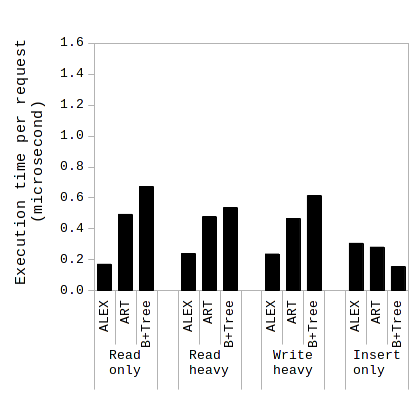
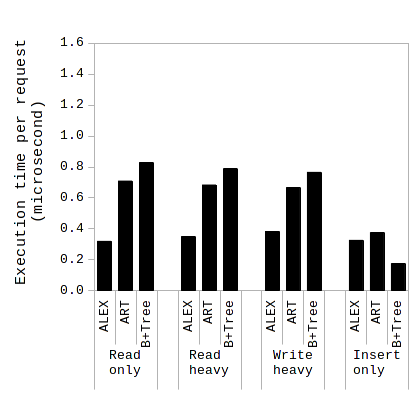
Figure 1 plots the execution time per request in $\mu$secs for all the experiments. Figure 1(a) and Figure 1(b) focus on the experiments, where the keys are consecutive from the given range as Section 3.3 detailed. Except for the insert-only workload, ALEX outperforms both ART and B+Tree in all workload cases, completing requests at least in half the time it takes for ART and B+Tree. This is as expected and corroborates the results from Ding et al. (Ding et al., 2020). The consecutive keys help with the model predictions, especially in read-only and read-heavy cases for ALEX.

On the other hand, inserting keys consecutively from out-of-bound values, is a costly operation for ALEX as the index has to expand the root. Normally, when ALEX expands a node, it either scales or retrains its model and then re-insert all the elements into the new expanded node based on the prediction of the scaled/retrained model. As described by Ding et al. (Ding et al., 2020), though, after some point, if ALEX realizes the append-only behavior in inserts, it stops model-based re-insertions, and just appends to the expanded space. The advantage of this is to avoid, re-modeling and re-inserting frequently. This routine leads to interesting micro-architectural behavior, as the following subsections will cover.

Overall, while the average execution time per request decreases as we increase the insert in ART and B+Tree in the consecutive case, we do not observe this for ALEX, whose relative performance becomes similar to or worse than ART and B+Tree. In addition, the increase in data size, cause an increase in the average execution time for requests for each index, which is expected as more data is traversed.

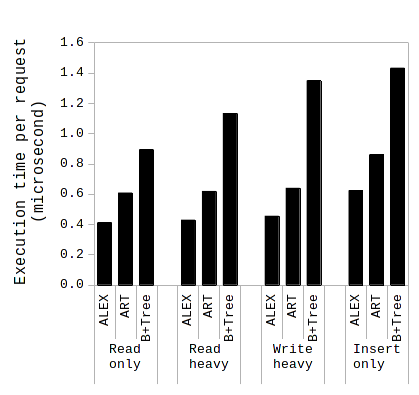
In the case of random routine, Figure 1(c), where the initial key range and later inserts are all randomly done from a given range, we observe a different trend. ALEX always outperforms the other two indexes and shows fairly stable performance across different workloads, except for a slight increase in the average execution time for the insert-only workload. Compared to the consecutive dataset, the overall execution time is slightly higher for ALEX with random keys. We see similar trends for B+Tree, but its average execution time per request exhibits a performance hit with random keys. For ART, on the other hand, except for the random insert-only workload, the average execution time per request is lower in the random case if we compare results for 1.6 billion keys from Figure 1(b) and Figure 1(c).

In the random scenario, the workloads with read requests have a non-negligible possibility of requesting a key that does not exist in the index (see Section 3.3). Therefore, this pattern leads to higher execution time per request in ALEX in two ways. First, the models could be less precise due to more random distribution of keys. Second, we pay the penalty of increased number of exponential search routines for non-existing keys compared to random read request in Figure 1(b). In addition, in the case of ART, we know that a successful search in radix trees is slower than an unsuccessful one as mentioned by Leis et al. (Leis et al., 2013). This explains ART’s opposite behavior compared to ALEX and B+Tree in this scenario.

(a) Consecutive - 160 million keys

(b) Consecutive - 1.6 billion keys

(c) Random - 1.6 billion keys

Figure 2. Instructions retired per request.

4.1.3. Instructions retired per request

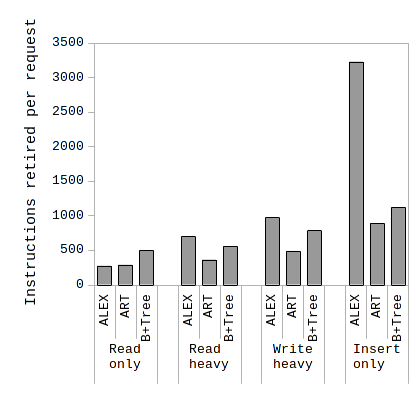
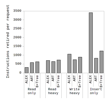
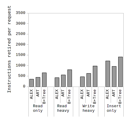
Figure 2 has the instructions retired per request across all experiments to give an idea of the instruction footprint of the three indexes. What jumps out from Figure 2(a) and Figure 2(b) is that on average ALEX has an order of magnitude increase in the number of instructions it uses to complete an out-of-bound insert request compared to a read operation. This is due to retraining of the model after so many inserts in the workload. Even if ALEX stops re-modeling and re-inserting after detecting the append-only pattern as mentioned in Section 4.1.2, it may have already performed a model update before that stop happens. As a result, this impacts the average execution time as well as average instruction footprint of such insert operations. On the other hand, as we will see in Figure 3 in the next section, these instructions exhibit a high instruction-level parallelism, which, in turn, prevents a drastic increase in the overall execution time as we see in Figure 1.

Overall, the increase in the % of inserts in the workload increase the instruction footprint for all indexes, but the impact is not as drastic as it is in the case of ALEX. In addition, for the case of random inserts, presented in Figure 2(c), ALEX also gets effected less as the overheads of such inserts can be prevented by the gapped array structure.

When comparing Figure 2(a) and Figure 2(b), we also observe that increasing the initial index size 10-fold naturally has impact on instruction footprint per request, as it may take longer time to traverse the tree. This impact is not very high in most cases, except for ART, where it doubles the instructions retired per request for read-only and read-heavy workloads.

(a) Consecutive - 160 million keys

(b) Consecutive - 1.6 billion keys

(c) Random - 1.6 billion keys

Figure 3. Cycles per Instruction - CPI (theoretical minimum is 0.25 on our server).

4.1.4. Cycles per instruction (CPI)

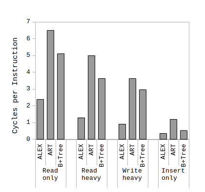
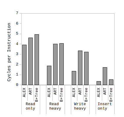
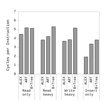
Figure 3 shows the cycles spent retiring an instruction on average across all the experiments. The smaller this value is the better, indicating that the processor core can exploit more instruction-level parallelism issuing and retiring more instructions in a cycle (Section 2.2). On the server we are using for these experiments, the minimum for this value is 0.25 as mentioned in Section 3.4.

Data-intensive applications, especially transaction processing applications, are famous for exhibiting low instruction-level parallelism (Section 2.3). The reason for this, especially for modern in-memory-optimized systems, is that frequent random data accesses lead to long-latency stalls trying to fetch data all the way down from main memory, when they do not hit in the L1 data cache. In addition, the complex instruction footprint of traditional disk-based data management systems cause high front-end stalls.

ALEX, ART, and B+Tree are all in-memory index structures targeting transaction processing workloads. They do not encapsulate all the instruction complexity for a data management system, since they just represent part of a data management system. On the other hand, index operations are the most common operations for most transactional workloads. Therefore, our expectation is to observe similar micro-architectural trends to in-memory transaction processing systems with heavy instruction footprint optimizations (as in HyPer results from (Sirin et al., 2016)) here and in the following subsections that detail the micro-architectural behavior.

Results from Figure 3 demonstrate that ALEX exhibit the highest level of instruction-level parallelism across all the experiments compared to ART and B+Tree. This corroborates the fundamental design principle for learned tree indexes, where a trade-off for increased computation is made instead of memory accesses (Bailis et al., 2018). Especially, with the insert-only workload inserting consecutive keys (Figure 3(a) and Figure 3(b)), ALEX comes very close to the theoretical minimum with a CPI value of 0.36. This is reasonable as the large instruction footprint reported in Section 4.1.3 is mainly computation heavy, which does not lead to too many data fetches from main-memory. In addition, both model training and possible later append operations do not exhibit complex program logic that could leave branch predictors and next-line prefetching in modern processors ineffective.

(a) Consecutive - 160 million keys

(b) Consecutive - 1.6 billion keys

(c) Random - 1.6 billion keys

Figure 4. Breakdown of execution cycles (normalized).

(a) Consecutive - 160 million keys

(b) Consecutive - 1.6 billion keys

(c) Random - 1.6 billion keys

Figure 5. Breakdown of back-end stalls (normalized).

For workloads with high percentage of reads or for random insert patterns, all three indexes spend more cycles per instruction as a result of increased random data fetches in a unit of time. This is a natural side-effect of a tree-index traversal, which the results from the following subsections will further corroborate.

The reduction in CPI for read-only and read-heavy workloads as the data size is increased (comparing Figure 2(a) and Figure 2(b)) also underlies the effect of traditional index traversal in ART and B+Tree. The way these tree-based indexes are designed, the level of the trees do not increase proportionally to the data size avoiding proportional increase in random data access requests to main-memory. Furthermore, the traversal code is also a tight-loop with relatively small instruction footprint that can be kept in the L1 instruction cache. These two fundamental characteristics of tree-based structures benefit the scalability with respect to data size for all three indexes. On the other hand, CPI for ALEX increases for the same scenario, while still being smaller than the other two indexes as a result of the trade-offs mentioned above. This is likely the impact of traversing a deeper hierarchy of models with the larger dataset.

We also see the positive impact of data locality for ART and B+Tree in the insert-only workload when comparing the consecutive (Figure 3(b)) and random (Figure 3(c)) inserts.

Finally, overall, the trends in Figure 1 and Figure 3 match for the cases of the large dataset sizes, and can be explained with similar reasoning. On the other hand, for the small dataset size, despite exhibiting a high CPI value, ART has more efficient execution time per request compared to the B+Tree, which may come as a result of its lower instruction footprint per request in Figure 2.

4.2. Breakdown of execution cycles

Section 4.1 demonstrated the top-level performance comparison across ALEX, ART, and B+Tree. While interpreting the results from the top-level metrics, we already hinted at certain causes at the micro-architectural-level for the observed behavior. Now, in this and the following two subsections, we quantify such causes in more detail.

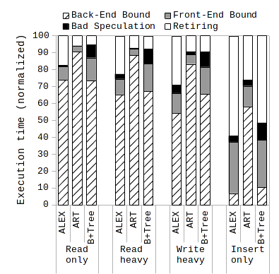
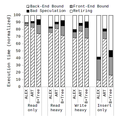
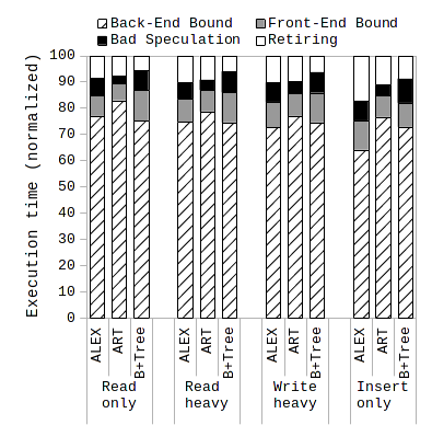
Figure 4 plots the breakdown of execution cycles into top-level micro-architectural components for all the experiments. We normalize the cycles to 100% and report the breakdowns in terms of percentages instead of absolute values, since Section 4.1.2 already compared the execution time for all three indexes in absolute values. Later, before closing our analysis of the experimental results, Section 4.4 also gives a detailed breakdown of the execution cycles over the absolute execution time without normalizing, to circle back to the results presented earlier.

With the expected exception of the insert-only workload with consecutive pattern, Figure 4 emphasizes that majority of the execution time for all index structures goes to back-end stalls. The time spent in retiring instructions is relatively small, as well as the stalls due to bad speculation and front-end. This behavior is expected, since index operations are data access heavy, leading to many random data accesses to main-memory (as Section 4.4 will further underline).

The portion of execution time ALEX spends in retiring instructions increases as the workload exhibits more out-of-bound inserts (Figure 4(a) and Figure 4(b)) as well as the front-end component. This is expected looking at the instructions required per request in Figure 2 for the same cases.

Overall, ALEX spends a smaller percentage of its execution time in back-end stalls compared to ART across all the experiments and percentage of back-end stalls is similar between ALEX and B+Tree. However, B+Tree spends a higher portion of time in front-end stalls and bad speculation. In terms of more stable or robust micro-architectural behavior, though, ART’s behavior does not change drastically across the experiments, even with the extreme case of the insert-only workload with consecutive out-of-bound inserts. ART is the most back-end bound compared to the other two indexes. This can be attributed to both its larger memory footprint (Section 4.1.1) and small instruction footprint (Section 4.1.3) increasing the pressure on the back-end of a processor.

Finally, for the random case illustrated in Figure 4(c), we do not see drastic changes in the behavior of the breakdown across different workload patterns. Here the random data accesses are simply the core operation all the indexes perform, which leads to this outcome.

4.3. Breakdown of back-end stalls

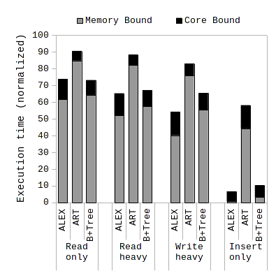
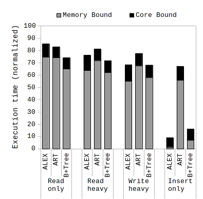
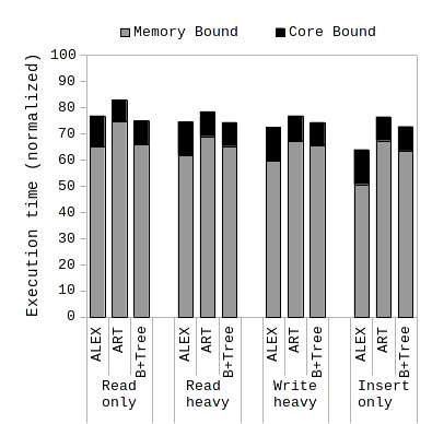
Since the execution cycles are mainly back-end bound in Figure 4, Figure 5 breaks down the back-end stalls further into memory bound and core bound components for all the experiments. Figure 5 keeps the total execution time normalized at 100%, while the total of the memory bound and core bound components sums up to the back-end bound component from Figure 4.

As expected, except for the case of out-of-bound inserts, majority of the back-end stalls are memory bound, because of the random data accesses. In addition, while small, the core bound component tends to be bigger for ALEX, because of the more compute-heavy nature of learned indexes. This may cause slightly increased pressure on the execution units in the back-end.

For the case of out-of-bound inserts (Figure 5(a) and Figure 5(b)), ALEX spends almost no time in memory bound stalls, which is interesting to observe and highlights the extremely compute-heavy nature of model re-training triggered by this workload pattern. B+Tree exhibits the impact of data locality in this case, whereas ART’s lower instruction and larger data footprint keeps the memory bound component big.

Finally, the trends across different dataset sizes and data insert patterns, aligns with the insights we had for the CPI results in Figure 3, and can be attributed to the index traversal logic as explained in Section 4.1.4. To re-iterate, the random inserts (Figure 5(c)) as well as random read requests (read-only and read-heavy), are bound by the impact of the random data accesses. Increasing the data size leads to more cache locality in both instruction and data accesses for the tree-based index structures that are not based on models such as ART and B+Tree. On the other hand, the increased number of models in ALEX with the increased data size leads to an increased memory bound behavior.

(a) Consecutive - 160 million keys

(b) Consecutive - 1.6 billion keys

(c) Random - 1.6 billion keys

Figure 6. Breakdown of memory stalls (normalized).

(a) Consecutive - 160 million keys

(b) Consecutive - 1.6 billion keys

(c) Random - 1.6 billion keys

Figure 7. Breakdown of memory stalls per request in $\mu$sec.

4.4. Breakdown of memory stalls

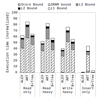
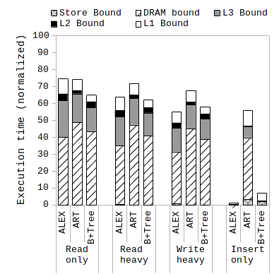
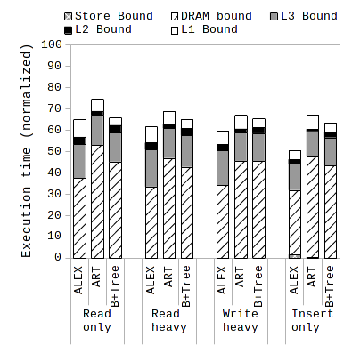
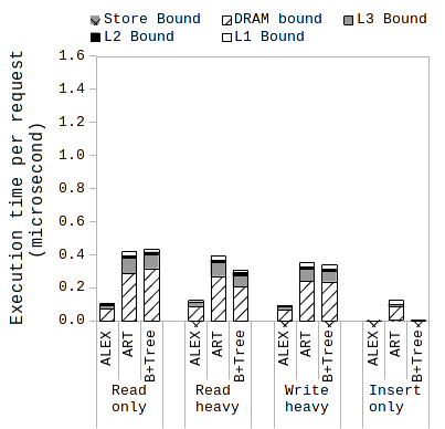
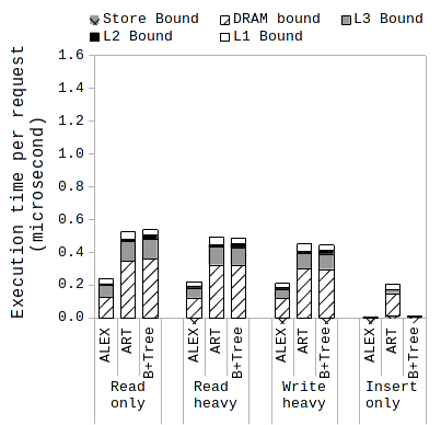
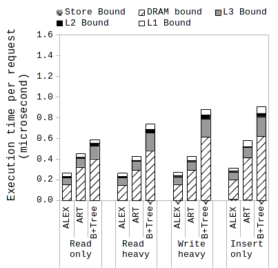
Since the back-end bound cycles are mainly memory bound in Figure 5, in this section, we break the memory bound stalls further into where they come from within the memory hierarchy. This section illustrates the results in two forms. First, Figure 6 plots this breakdown with respect to normalized execution time. This means that the total of the presented components in Figure 6 sums up to the memory bound component from Figure 5. Then, Figure 7 shows this breakdown with respect to the absolute values for the execution time from Figure 1 presenting the absolute time for various memory bound stalls per request. This also allows us to circle back to the top-level performance metrics we presented earlier this section. The y-axes in Figure 7 is, therefore, kept the same as the results in Figure 1 for better comparison.

Figure 6 demonstrates that majority of the memory bound stalls are due to long-latency data misses from the last-level cache (L3), which is labeled as DRAM bound, for all indexes. This is followed by the data misses from L2 cache that hit in L3 cache, which the L3 Bound component represents. In contrast, L2 Bound component, which shows stall time due to L1 data cache misses, is quite small as well as the L1 Bound component, which is mostly due to DTLB misses in our case.

This behavior of the memory stalls can be explained through both the hardware and software behavior. On the one hand, modern OoO processors are designed to overlap the latency for the L1 data misses for the most part, which is 7-8 cycles. However, the latency for L2 and L3 misses are larger (17 and over 200 cycles, respectively). Therefore, it becomes hard to overlap all the associated latency due to frequent random data accesses to L3 and DRAM. On the other hand, the tree-based index traversal logic triggered by the get/put/update requests to indexes in our (and typical transactional) workloads, exhibit very low temporal and spatial locality leading to many cache misses from all levels of the cache hierarchy. Therefore, except for the accesses to the higher-levels of the index (e.g., root), most data accesses end up in DRAM.

The case that shows different behavior is again the out-of-bound inserts in Figure 6(a) and Figure 6(b). ALEX and B+Tree exhibit almost no stalls due to memory accesses here as Section 4.3 also covered.

Finally, Figure 7 shows that, in absolute values, ALEX spends the least amount of time in memory bound stalls compared to ART and B+Tree, which aligns with its normalized values as well. On the other hand, ART and B+Tree spend similar amount of time in memory bound stalls in consecutive case, while ART spends shorter time in memory bound stalls in random case, despite the normalized values in Figure 6. This is a result of ART’s more efficient utilization of the front-end component, which is very small for ART in the normalized case, increasing the impact and portion of the memory bound. Therefore, it is important to have both the normalized and absolute perspectives while breaking down the execution cycles into micro-architectural components.

5. Conclusion

In this paper, we performed a micro-architectural analysis of a learned index, ALEX, and compared its behavior to two tree-based indexes that are not based on learned models, ART and B+Tree. Our study complements existing experimental comparison results for learned indexes by providing a lower-level view of how well learned indexes utilize the front-end, back-end, memory hierarchy, etc. of modern commodity servers with OoO processors.

We used a variety of workloads with different % of read and write requests as well as different data insert and access patterns and sizes. In summary, our results show that, long-latency data misses is at the core of ALEX similar to the other two indexes. This is expected as the short get/put requests cause frequent random data accesses that lack locality, which stress the memory hierarchy of a processor. On the other hand, ALEX exhibits higher instruction-level parallelism and fewer stalls cycles in general. This is a result of the fact that learned indexes trade-off increased computations to reduced memory accesses, which could boost performance if the overall computation cycles are cheaper with respect to memory access latency (Bailis et al., 2018). In the case of modern OoO processors, computation cycles are indeed cheaper if the instruction footprint is not complex, i.e., does not have too many dependencies. Even if ALEX’s instruction footprint drastically increases in the case of inserting out-of-bound keys, these instructions are less stall prone, since they exhibit very high instruction-level parallelism.

Going forward, investigating the behavior for the same index structures for workload patterns that dynamically change over time during a single run would be interesting to observe the impact of various insert heavy periods on later read heavy periods of execution. In addition, in this study we mainly looked at uniformly random data access patterns. Adopting a variety of access patterns as well as more complex insert behavior would also be an interesting future analysis.

Acknowledgements

The authors would like to thank Intel DevCloud (DevCloud, [n. d.]) for providing the server and the maintainers of the open-source codebases used used by the experiments in this paper.

References

- (1)
- Ailamaki et al. (1999) Anastassia Ailamaki, David J. DeWitt, Mark D. Hill, and David A. Wood. 1999. DBMSs on a Modern Processor: Where Does Time Go?. In VLDB. 266–277.
- Awan et al. (2016) Ahsan Javed Awan, Mats Brorsson, Vladimir Vlassov, and Eduard Ayguade. 2016. Micro-Architectural Characterization of Apache Spark on Batch and Stream Processing Workloads. In BDCloud-SocialCom-SustainCom. 59–66.
- Bailis et al. (2018) Peter Bailis, Kai Sheng Tai, Pratiksha Thaker, and Matei Zaharia. 2018. Don’t Throw Out Your Algorithms Book Just Yet: Classical Data Structures That Can Outperform Learned Indexes. (2018). https://dawn.cs.stanford.edu/2018/01/11/index-baselines/.
- Bingmann (2021) Timo Bingmann. Downloaded on March 15, 2021. STX B+ Tree Version 0.9. (Downloaded on March 15, 2021). https://panthema.net/2007/stx-btree/.
- Cooper et al. (2010) Brian F. Cooper, Adam Silberstein, Erwin Tam, Raghu Ramakrishnan, and Russell Sears. 2010. Benchmarking Cloud Serving Systems with YCSB. In ACM SoCC. 143–154.
- Crotty (2021) Andrew Crotty. 2021. Hist-Tree: Those Who Ignore It Are Doomed to Learn. In CIDR. 1–6.
- Dadgar (2021) Armon Dadgar. Forked on March 9, 2021. libart. (Forked on March 9, 2021). https://github.com/armon/libart.
- DevCloud ([n. d.]) Intel® DevCloud. [n. d.]. Intel® DevCloud: Remote Development Environments for Any Use Case. ([n. d.]). https://software.intel.com/content/www/us/en/develop/tools/devcloud.html.
- Ding (2021) Jialin Ding. Forked on February 16, 2021. ALEX. (Forked on February 16, 2021). https://github.com/microsoft/ALEX.
- Ding et al. (2020) Jialin Ding, Umar Farooq Minhas, Jia Yu, Chi Wang, Jaeyoung Do, Yinan Li, Hantian Zhang, Badrish Chandramouli, Johannes Gehrke, Donald Kossmann, David Lomet, and Tim Kraska. 2020. ALEX: An Updatable Adaptive Learned Index. In ACM SIGMOD. 969–984.
- Ferdman et al. (2012) Michael Ferdman, Almutaz Adileh, Onur Kocberber, Stavros Volos, Mohammad Alisafaee, Djordje Jevdjic, Cansu Kaynak, Adrian Daniel Popescu, Anastasia Ailamaki, and Babak Falsafi. 2012. Clearing the Clouds: A Study of Emerging Scale-out Workloads on Modern Hardware. In ASPLOS. 37–48.
- Ferragina and Vinciguerra (2020) Paolo Ferragina and Giorgio Vinciguerra. 2020. The PGM-Index: A Fully-Dynamic Compressed Learned Index with Provable Worst-Case Bounds. PVLDB 13, 8 (2020), 1162–1175.
- Galakatos et al. (2019) Alex Galakatos, Michael Markovitch, Carsten Binnig, Rodrigo Fonseca, and Tim Kraska. 2019. FITing-Tree: A Data-Aware Index Structure. In ACM SIGMOD. 1189–1206.
- Graefe (2011) Goetz Graefe. 2011. Modern B-Tree Techniques. Found. Trends Databases 3, 4 (2011), 203–402.
- Hadian and Heinis (2021) Ali Hadian and Thomas Heinis. 2021. Shift-Table: A Low-latency Learned Index for Range Queries using Model Correction. In EDBT. 253–264.
- Hardavellas et al. (2007) Nikos Hardavellas, Ippokratis Pandis, Ryan Johnson, Naju G. Mancheril, Anastassia Ailamaki, and Babak Falsafi. 2007. Database Servers on Chip Multiprocessors:Limitations and Opportunities. In CIDR. 79–87.
- Intel® ([n. d.]a) Intel®. [n. d.]a. Clockticks Vs. Pipeline Slots Based Metrics. ([n. d.]). https://software.intel.com/content/www/us/en/develop/documentation/vtune-help/top/reference/cpu-metrics-reference/clockticks-vs-pipeline-slots-based-metrics.html.
- Intel® ([n. d.]b) Intel®. [n. d.]b. Instrumentation and Tracing Technology APIs. ([n. d.]). https://software.intel.com/content/www/us/en/develop/documentation/vtune-help/top/api-support/instrumentation-and-tracing-technology-apis.html.
- Intel® ([n. d.]c) Intel®. [n. d.]c. Intel® VTune™ Profiler. ([n. d.]). https://software.intel.com/content/www/us/en/develop/tools/oneapi/components/vtune-profiler.html.
- Intel® ([n. d.]d) Intel®. [n. d.]d. Top-down Microarchitecture Analysis Method. ([n. d.]). https://software.intel.com/content/www/us/en/develop/documentation/vtune-cookbook/top/methodologies/top-down-microarchitecture-analysis-method.html.
- Kanev et al. (2015) Svilen Kanev, Juan Pablo Darago, Kim Hazelwood, Parthasarathy Ranganathan, Tipp Moseley, Gu-Yeon Wei, and David Brooks. 2015. Profiling a Warehouse-Scale Computer. In ISCA. 158–169.
- Keeton et al. (1998) K. Keeton, D.A. Patterson, Yong Qian He, R.C. Raphael, and W.E. Baker. 1998. Performance characterization of a quad Pentium Pro SMP using OLTP workloads. In ISCA. 15–26.
- Kipf et al. (2019) Andreas Kipf, Ryan Marcus, Alexander van Renen, Mihail Stoian, Alfons Kemper, Tim Kraska, and Thomas Neumann. 2019. SOSD: A Benchmark for Learned Indexes. MLForSystems@NeurIPS (2019).
- Kipf et al. (2020) Andreas Kipf, Ryan Marcus, Alexander van Renen, Mihail Stoian, Alfons Kemper, Tim Kraska, and Thomas Neumann. 2020. RadixSpline: A Single-Pass Learned Index. In aiDM@SIGMOD. 5:1–5:5.
- Kowalski et al. (2020) Thomas Kowalski, Fotios Kounelis, and Holger Pirk. 2020. High-Performance Tree Indices: Locality matters more than one would think. In ADMS. 1–6.
- Kraska et al. (2018) Tim Kraska, Alex Beutel, Ed H. Chi, Jeffrey Dean, and Neoklis Polyzotis. 2018. The Case for Learned Index Structures. In ACM SIGMOD. 489–504.
- Leis et al. (2013) Viktor Leis, Alfons Kemper, and Thomas Neumann. 2013. The Adaptive Radix Tree: ARTful Indexing for Main-Memory Databases. ICDE, 38–49.
- Levandoski et al. (2013) Justin Levandoski, David Lomet, and Sudipta Sengupta. 2013. The Bw-Tree: A B-tree for New Hardware Platforms. In ICDE.
- manual page ([n. d.]) Linux manual page. [n. d.]. top. ([n. d.]). https://man7.org/linux/man-pages/man1/top.1.html.
- Marcus et al. (2020) Ryan Marcus, Andreas Kipf, Alexander van Renen, Mihail Stoian, Sanchit Misra, Alfons Kemper, Thomas Neumann, and Tim Kraska. 2020. Benchmarking Learned Indexes. PVLDB 14, 1 (2020), 1–13.
- Nathan et al. (2020) Vikram Nathan, Jialin Ding, Mohammad Alizadeh, and Tim Kraska. 2020. Learning Multi-Dimensional Indexes. In ACM SIGMOD. 985–1000.
- Ranganathan et al. (1998) Parthasarathy Ranganathan, Kourosh Gharachorloo, Sarita V. Adve, and Luiz André Barroso. 1998. Performance of Database Workloads on Shared-Memory Systems with out-of-Order Processors. In ASPLOS. 307–318.
- Sirin and Ailamaki (2020) Utku Sirin and Anastasia Ailamaki. 2020. Micro-architectural Analysis of OLAP: Limitations and Opportunities. PVLDB 13, 6 (2020), 840–853.
- Sirin et al. (2016) Utku Sirin, Pinar Tözün, Danica Porobic, and Anastasia Ailamaki. 2016. Micro-architectural Analysis of In-memory OLTP. In ACM SIGMOD. 387–402.
- Sirin et al. (2021) Utku Sirin, Pinar Tözün, Danica Porobic, Ahmad Yasin, and Anastasia Ailamaki. 2021. Micro-architectural Analysis of In-memory OLTP: Revisited. (2021), 1–25.
- Sirin et al. (2017) Utku Sirin, Ahmad Yasin, and Anastasia Ailamaki. 2017. A methodology for OLTP micro-architectural analysis. In DaMoN @ ACM SIGMOD. 1:1–1:10.
- Stets et al. (2002) Stets, Gharachorloo, and Barroso. 2002. A Detailed Comparison of Two Transaction Processing Workloads. In IEEE WWC. 37–48.
- Tözün et al. (2013) Pınar Tözün, Ippokratis Pandis, Cansu Kaynak, Djordje Jevdjic, and Anastasia Ailamaki. 2013. From A to E: Analyzing TPC’s OLTP Benchmarks: The Obsolete, the Ubiquitous, the Unexplored. In EDBT. 17–28.
- Yasin (2014) Ahmad Yasin. 2014. A Top-Down method for performance analysis and counters architecture. In ISPASS. 35–44.
- Yasin et al. (2014) Ahmad Yasin, Yosi Ben-Asher, and Avi Mendelson. 2014. Deep-dive analysis of the data analytics workload in CloudSuite. In IISWC. 202–211.