Arbitrary-precision computation of the gamma function

Abstract.

We discuss the best methods available for computing the gamma function $\Gamma(z)$ in arbitrary-precision arithmetic with rigorous error bounds. We address different cases: rational, algebraic, real or complex arguments; large or small arguments; low or high precision; with or without precomputation. The methods also cover the log-gamma function $\log\Gamma(z)$, the digamma function $\psi(z)$, and derivatives $\Gamma^{(n)}(z)$ and $\psi^{(n)}(z)$. Besides attempting to summarize the existing state of the art, we present some new formulas, estimates, bounds and algorithmic improvements and discuss implementation results.

1. Introduction

The gamma function

$$\Gamma(z)=\int_{0}^{\infty}t^{z-1}e^{-t}dt\quad(\operatorname{Re}(z)>0),\quad\Gamma(z)=\frac{\Gamma(z+1)}{z},$$ (1)

is arguably the most important higher transcendental function, having a tendency to crop up in any setting involving sequences, series, products or integrals when the solutions go beyond elementary functions.

Calculation of the gamma function is a classical subject in numerical analysis. The standard algorithm uses the asymptotic Stirling series

$$\Gamma(z+1)\,=\,z!\;\sim\;\sqrt{2\pi}\,e^{-z}z^{z+1/2}\left(1+\frac{1}{12z}+\frac{1}{288z^{2}}+\ldots\right),\quad|z|\to\infty,$$ (2)

which is valid in every closed sector of the complex plane excluding the negative real line. If $z$ is too small or too close to the negative real line to use (2) directly, one first applies a shift $z\to z+r$ and possibly the reflection formula

$$\Gamma\!\left(z\right)=\frac{\pi}{\sin\!\left(\pi z\right)}\frac{1}{\Gamma\!\left(1-z\right)}.$$ (3)

The story does not end here: a close study of the Stirling series presents a number of interesting theoretical problems and implementation issues, and there are also many alternative algorithms. However, despite an extensive literature on gamma function computation, there have been surprisingly few attempts to investigate the best available techniques from the point of view of arbitrary-precision computation. It seems worthwhile to pursue this topic since some applications require repeated evaluation of $\Gamma(z)$ to a precision of hundreds or thousands of digits.

1.1. Quick survey of methods

It is convenient to sort algorithms for the gamma function into four broad categories.

1. Global methods approximate $\Gamma(z)$ in the whole complex plane using its asymptotics together with a correction. The Stirling series and the formulas of Lanczos [Lan64] and Spouge [Spo94] are all of this type.

2. Local methods approximate the gamma function near particular points or on particular intervals such as $z\in[1,2]$ using tabulated values, Taylor series, Chebyshev interpolants, or other approximations.

3. Hypergeometric methods represent the gamma function in terms of hypergeometric functions which may be evaluated using series expansions.

4. Integration methods evaluate (1) or a suitable contour integral using standard numerical integration techniques.

The different categories all have their uses. Global methods are the most broadly useful, but local methods can perform better where they are applicable. The main drawback of the local methods is their high precomputation cost. The hypergeometric methods are the most efficient asymptotically at high precision due to the possibility to use complexity-reduction techniques.

Table 1 lists some of the major algorithms along with estimates of the rate of convergence, expressed as the number of terms needed asymptotically to achieve $p$-bit accuracy. This rate cannot be taken as a direct measure of efficiency, because the notion of “term” differs between the algorithms:

• The “generic” terms require at least a full multiplication and possibly additional work, some of which may be subject to precomputations.

• The “hypergeometric” terms asymptotically require less than a full multiplication. The precise amount of work varies depending on the formula.

Table 1. Algorithms for the gamma function. Where no reference is given, the convergence rate estimates will be justified below.

Formula	Needed terms for $p$-bit accuracy	Type of terms
Global methods (any $z$)
Stirling series	$0.323p$ (worst case)	Generic/hypergeometric
Spouge’s formula	$0.377p$ (uniformly)	Generic
	$<0.225p$ (small $z$, conjectured)
Lanczos’s formula	unknown	Generic
Binet convergent series	$1.00p$ (worst case)	Generic
Stieltjes continued fraction	$0.323p$ (worst case, conjectured)	Generic
Local methods ($|z|\ll p$)
Taylor series	$O(p/\log(p))$	Generic
Chebyshev interpolants	$O(p/\log(p))$	Generic
Hypergeometric methods ($|z|\ll p$)
Incomplete gamma functions	$1.49p$	Hypergeometric
Bessel functions	$1.09p$	Hypergeometric
Elliptic integrals	$O(\log p)$ (special $z$ only)	Generic
Integration methods
Contour integration	$0.311p$ (conjectured) [ST07]	Generic

The performance of different algorithms also sometimes depends strongly on whether $z$ is an integer, rational, algebraic, real or complex number, or a power series with the respective types of coefficients. Despite these variables, the rate of convergence is useful as a first point of reference. A more detailed comparison will be one of the goals of this study.

Integration methods are the only class that will not be studied here; the reader may instead refer to Schmelzer and Trefethen [ST07]. Despite potentially very rapid convergence, numerical integration is unlikely to be competitive with more specialized algorithms due to requiring repeated evaluations of a transcendental integrand. Direct integration has one major advantage: it is easy to generalize to other functions. The integral (1) is the Laplace transform of $t^{z-1}$ as well as the Mellin transform of $e^{-t}$; it is clearly interesting to have efficient schemes for evaluation of similar integrals when no convenient closed form is available.

Notably missing from the list is solving an ordinary differential equation. Indeed, the gamma function itself does not satisfy any algebraic differential equation with polynomial coefficients (Hölder’s theorem [Höl86]). In the hypergeometric methods, the gamma function is effectively viewed as the connection coefficient between the formal solutions of a differential equation at two singular points, but here $z$ appears as a parameter of the differential equation, not as the integration variable. The lack of a “nice” differential equation precludes asymptotically fast techniques available for many other functions such as elementary functions, $\operatorname{erf}(z)$, Bessel functions $J_{n}(z)$, etc. (technically, holonomic or D-finite functions [vdH99, Mez11]).

1.2. Contents and contributions

This work is structured as follows. Section 2 reviews notation, formulas, precision issues and implementation techniques which are common to all algorithms for the gamma function.

Section 3 treats the Stirling series in depth. We give pseudocode and discuss error bounds, precision loss, parameter choices, convergence rates, and implementation techniques. The most interesting contribution is an improvement to the Stirling series (Theorem 3.5 and Algorithm 6) which simultaneously improves performance and requires fewer Bernoulli numbers (this leads to the fastest known general method for computing the gamma function up to about $10^{6}$ digits).

Section 4 discusses global alternatives to the Stirling series. We analyze the efficiency of several algorithms and attempt to answer whether the Stirling series should be dethroned. (Spoiler: it should not.)

Section 5 discusses local methods. Our main contribution is to analyze computation using Taylor series. Our results include a simple lower bound for the complex gamma function (Theorem 5.1) which is new or at least does not appear in any of the usual reference works, and new, improved bounds for Taylor coefficients of the reciprocal gamma function (Theorem 5.2 and formula 71).

Section 6 discusses reduced-complexity methods using hypergeometric series. We provide a comprehensive collection of hypergeometric representations of the gamma function and analyze their efficiency. Section 7 presents benchmark results for multiple algorithms, and section 8 discusses open problems.

Most of the algorithms have been implemented in Arb [Joh17]. This study was prompted by a rewrite of gamma and related functions in Arb undertaken by the author in 2021, for which we wanted to explore plausible alternative algorithms and new optimizations. The work builds on, but significantly expands and updates, results reported in the thesis [Joh14b].

2. General techniques and preliminaries

2.1. Variants of the gamma function

A number of variants of $\Gamma(z)$ appear in applications and may be provided as standalone functions in software:

• The factorial $z!$, which avoids a sometimes awkward shift by one.

• The reciprocal gamma function $1/\Gamma(z)$, which is an entire function and avoids issues with division by zero at the poles of $\Gamma(z)$ at $z=0,-1,\ldots$. This function is also useful in situations where $\Gamma(z)$ risks overflowing (where $1/\Gamma(z)$ can evaluate to an upper bound or underflow to zero).

• The scaled gamma function $\Gamma^{*}(z)=(2\pi)^{-1/2}e^{z}{z}^{1/2-z}\Gamma(z)$, which by (2) satisfies $\Gamma^{*}(z)\to 1$ when $z\to+\infty$, avoiding overflow and conditioning issues for large arguments [GST07, Nem15].

• The log-gamma function $\log\Gamma(z)$, whose principal branch is defined to be holomorphic at $+\infty$ with branch cuts on the negative real axis, continuous from above. The log-gamma function is useful for large arguments (avoiding overflow and conditioning issues) and for turning products or quotients of gamma functions into sums; some applications also require $\log\Gamma(z)$ itself.

• The digamma function $\psi(z)=d/dz\,\log\Gamma(z)=\Gamma^{\prime}(z)/\Gamma(z)$.

• The derivatives $\Gamma^{(n)}(z)$, $[1/\Gamma(z)]^{(n)}$ and $\psi^{(n)}(z)$. The functions $\psi^{(n)}(z)$ are also known as polygamma functions.

Algorithms for the functions listed above are closely related if not interchangeable. In particular, any algorithm for $\Gamma(z)$ can be differentiated to obtain the derivatives $\Gamma^{(n)}(z)$, $\psi^{(n)}(z)$, etc. This is sometimes best done by differentiating formulas manually, but in many cases, we can simply implement the original formulas using automatic differentiation; that is, we take $z$ to be a truncated power series

$$z=c_{0}+c_{1}x+\ldots+c_{n}x^{n}\;\in\;\mathbb{C}[[x]]\langle x^{n+1}\rangle.$$ (4)

When used with fast power series arithmetic (based on FFT multiplication), this also typically yields the best complexity for computing high-order derivatives.

Algorithms for the gamma function also permit the computation of rising factorials (Pochhammer symbols), falling factorials, binomial coefficients, and the beta function. Some techniques are applicable to incomplete gamma and beta functions, the Barnes $G$-function, the Riemann zeta function, and other special functions. To keep the scope manageable, we will not consider such functions except where they are involved in calculating the gamma function itself.

The gamma function can be defined for a matrix argument. In general, the scalar algorithms can be generalized to the matrix case; see [CS19a, Miy20]. For the $p$-adic analog of the gamma function, see [Vil07].

2.2. Precision, accuracy and complexity

Except where otherwise noted, $p$ either denotes a precision in bits (meaning that real and complex numbers are represented by $p$-bit floating-point approximations) or a target accuracy (meaning that we target a relative error of order $2^{-p}$). For an introduction to arbitrary-precision arithmetic and many of the underlying algorithms and implementation techniques, see Brent and Zimmermann [BZ11].

We typically need some extra bits of working precision for full $p$-bit accuracy, where the precise amount depends on the input and on the algorithm. We will analyze sources of numerical error in some cases, but we will not attempt to write down explicit bounds for errors resulting from floating-point rounding. Most algorithms can be implemented in ball arithmetic [vdH09, Joh17] to provide rigorous error bounds. To compute the gamma function with a guaranteed relative error $2^{-p}$, it thus suffices to choose a working precision $p^{\prime}>p$ heuristically; we can restart with increased precision in the rare event that the heuristic estimate turns out to be inadequate, and any complexity analysis only depends on the estimate for $p^{\prime}$ being accurate asymptotically.

To guarantee correct rounding, Ziv’s strategy [Ziv91, MBdD⁺18] should be used: we compute a first approximation with a few guard bits and restart with increased precision if the correctly rounded result cannot be determined unambiguously. To ensure termination, this loop needs to be combined with a test for input $z$ where $\Gamma(z)$ is exactly representable, which (in the case of floating-point input $z$) conjecturally occurs only for $z\in\mathbb{Z}$. For efficiency reasons, certain limiting cases should also be handled specially (e.g. $\Gamma(z)\sim 1/z-\gamma$, $z\to 0$).

We will state some complexity bounds in the form $\widetilde{O}(n)$, meaning $O(n\log^{c}n)$ where we do not care about the constant $c$. Arithmetic complexity bounds assume that operations have unit cost, while bit complexity bounds account for the cost of manipulating $p$-bit numbers in the multitape Turing model. Additions and subtractions cost $O(p)$ bit operations while multiplications cost $M(p)=O(p\log p)=\widetilde{O}(p)$ with the asymptotically fastest known algorithm [HvdH21]. Divisions and square roots cost $O(M(p))$ and elementary functions cost $O(M(p)\log p)$. For moderate number of bits $p$ (up to a few thousand, say), it is more accurate to estimate multiplications as having cost $O(p^{2})$ while elementary functions cost $O(p^{2.5})$.

We will sometimes use the fact that arithmetic operations and elementary functions can be applied to power series of length $n$ using $O(n\log n)=\widetilde{O}(n)$ arithmetic operations on coefficients. This does not always translate to a uniform bit complexity bound, because power series operations often lose $O(n)$ or $O(n\log n)$ bits of accuracy to cancellations (i.e. we will often need $p=\widetilde{O}(n)$).

2.3. Error propagation

In ball arithmetic or interval arithmetic, the input $z$ to a function $f$ may be inexact, i.e. it may be given by a rectangular enclosure $z\in[m\pm r]$, $z\in[a\pm r]+[b\pm s]i$ or a complex ball $z=D(m,r)$. We can let the uncertainty in the input propagate automatically through an algorithm that computes $f$, but this sometimes yields needlessly pessimistic enclosures.

A remedy is to evaluate $f$ at an exact floating-point number $m\in E$, typically the midpoint of $E$, where $E$ is the enclosure for $z$. We can then bound the propagated error using the radius of $E$ and an accurate bound for $\sup_{t\in E}|f^{\prime}(t)|$. Suitable bounds for derivatives of $\Gamma(z)$, $1/\Gamma(z)$ and $\log\Gamma(z)$ can be computed using the Stirling series or other global approximations that will be discussed later (machine-precision accuracy is sufficient for this).

When the input enclosures are wide, it is better to evaluate lower and upper bounds. The functions $\Gamma(x)$, $1/\Gamma(x)$, $\log\Gamma(x)$ are monotonic on the intervals $(0,x_{0}]$ and $[x_{0},\infty)$ where $x_{0}=1.4616\ldots$ while the functions $\psi^{(m)}(z)$ are monotonic on $(0,\infty)$. These conditions can be extended to segments on the negative real line via the reflection formula. In the complex domain, monotonicity conditions for the real and imaginary parts of $\Gamma(z)$ are more complicated; a convenient solution is to exponentiate an enclosure of $\log\Gamma(z)$.

2.4. Rising factorials

The shift relation $\Gamma(z+1)=z\Gamma(z)$ can be used in two ways: either to reduce the argument $z$ to a fixed strip near the origin, for example $1\leq\operatorname{Re}(z)\leq 2$ (useful for local and hypergeometric methods), or to ensure that $|z|$ or $\operatorname{Re}(z)$ is large (for use with asymptotic methods).

Let us now consider the problem of evaluating a repeated argument shift, i.e. computing the rising factorial

$$(z)_{n}\,=\,z(z+1)\cdots(z+n-1)\,=\,\frac{\Gamma(z+n)}{\Gamma(z)},\quad n\geq 0.$$ (5)

When $n$ is extremely large, the best way to compute $(z)_{n}$ numerically is to use asymptotic formulas for the gamma function or for $(z)_{n}$ itself, but our interest here is in smaller $n$ (of order $n\lesssim p^{1+\varepsilon}$) where we want to use rising factorials in the computation of the gamma function and not vice versa.

The rising factorial also serves as a model problem for the evaluation of hypergeometric series which will be considered later. We recall that a sequence $f(n)$ is hypergeometric if it satisfies a recurrence relation of the form $f(n+1)/f(n)=P(n)/Q(n)$ for some polynomials $P$, $Q$, or equivalently if $f(n)$ can be written as

$$f(n)=cd^{n}\frac{(a_{1})_{n}\cdots(a_{p})_{n}}{(b_{1})_{n}\cdots(b_{q})_{n}}.$$ (6)

for some constants $a_{1},\ldots,a_{p},b_{1},\ldots,b_{q},c,d$.

2.4.1. Binary splitting

The obvious, iterative algorithm to compute $(z)_{n}$ can in some circumstances be improved using a divide-and-conquer strategy.

Algorithm 1 Rising factorial using binary splitting

1:$z\in R$, $n\in\mathbb{N}$ where $R$ is any ring with $1\in R$

2:$z(z+1)\cdots(z+n-1)\in R$

3:if $n\leq 10$ then $\triangleright$ Tuning parameter

4:    return $z(z+1)\cdots(z+n-1)$ $\triangleright$ Direct iterative product

5:end if

6:$A\leftarrow(z)_{m},\;B\leftarrow(z+m)_{n-m}$,  $m=\lfloor n/2\rfloor$ $\triangleright$ Recursive calls

7:return $AB$

Algorithm 1 is typically more numerically stable than the iterative algorithm, particularly in rectangular complex interval arithmetic. Additionally, when $R=\mathbb{Q}$, its bit complexity is only $\widetilde{O}(n)$ compared to $\widetilde{O}(n^{2})$ for the iterative algorithm. A similar speedup occurs in many other rings with coefficient growth.

When $z\in\mathbb{Q}$, it is best to keep numerators and denominators unreduced and only canonicalize the final result. If we want $(z)_{n}$ as a numerical approximation rather than an exact fraction, no GCDs are needed at all. When $z\in\mathbb{Z}$ is a small integer; that is, when we are essentially computing $n!$, the basic binary splitting scheme can be improved by exploiting the prime factorization of factorials [Bor85, Lus08].

2.4.2. Rectangular splitting

The following algorithm [Joh14a] is better for $z\in R$ where a “nonscalar” (full) multiplication $xy$ with $x,y\in R$ has high, uniform cost while a “scalar” operation such as $x+cy$ is cheap. This assumption typically holds, for example, when $z$ is a $p$-bit real or complex number and $c\in\mathbb{Z}$ with $p\gg\log_{2}|c|$, when $z$ is a matrix, or when $z$ is a truncated power series.

Algorithm 2 Rising factorial using rectangular splitting

1:$z\in R$, $n\in\mathbb{N}$ where $R$ is any ring with $1\in R$

2:$z(z+1)\cdots(z+n-1)\in R$

3:Select tuning parameter $1\leq m\leq\max(n,1)$

4:Compute the powers $z^{2},z^{3},\ldots,z^{m}$

5:$k\leftarrow 0$

6:$r\leftarrow 1$

7:while $k<n$ do

8:    $\ell\leftarrow\min(m,n-k)$

9:    Expand $f=(X+k)\cdots(X+k+\ell-1)=\sum_{i=0}^{\ell}f_{i}X^{i}\in\mathbb{Z}[X]$

10:    $t\leftarrow f(z)=f_{0}+f_{1}z+\ldots+f_{\ell}z^{\ell}$ $\triangleright$ Using precomputed powers of $z$

11:    $r\leftarrow r\cdot t$

12:    $k\leftarrow k+m$

13:end while

14:return $r$

Algorithm 2 performs $O(n)$ scalar operations and $m+n/m$ full multiplications, where $m$ is a tuning parameter. The number of full multiplications is minimized if we take $m\approx\sqrt{n}$, giving roughly $2\sqrt{n}$ such multiplications. However, the cost also depends on the size of the coefficients $f_{i}$ and on implementation details, so the optimal $m$ must be determined empirically. For example, a carefully tuned implementation for $z\in\mathbb{R}$ in Arb uses $m=\lfloor\min(\sqrt{n},8+0.2\max(0,p-4096)^{0.4},60)\rfloor$ for $n>50$, and $m=1,2,4$ or $6$ for smaller $n$.

The polynomial $f$ can be constructed using repeated multiplication by linear polynomials, resulting in a triangular scheme for the coefficients. It can also be constructed using binary splitting (applied to a rising factorial in the ring $\mathbb{Z}[X]$), but for the degrees that will be encountered in gamma function computation, the triangular scheme suffices (it should be implemented using machine words when $n$ and $m$ are small enough that overflow cannot occur).

The scalar operations $\sum_{k}f_{k}z^{k}$ can be implemented using optimized code for dot products [Joh19b]. If $z$ is a truncated power series, the inner operations can be viewed as a matrix multiplication; the algorithm is related to the Brent-Kung algorithm [BK78] for power series composition.

2.4.3. Logarithmic rising factorial

Algorithm 3 Logarithmic rising factorial (with correct branches)

1:$z\in\mathbb{C}$ with $\operatorname{Im}(z)>0$, $n\in\mathbb{N}$

2:$\log\,(z)_{n}=\sum_{k=0}^{n-1}\log(z+k)$

3:$f\leftarrow z(z+1)\cdots(z+n-1)$ $\triangleright$ Using fast rising factorial algorithm

4:If $n\leq 1$, return $\log(f)$

5:$s\leftarrow z$,   $m\leftarrow 0$ $\triangleright$ Set $s$ to a floating-point approximation of $z$

6:for $k\leftarrow 1,2,\ldots,n-1$ do

7:    $t\leftarrow s\cdot(z+k)$ $\triangleright$ Approximate floating-point product

8:    if $\operatorname{Im}(s)\geq 0$ and $\operatorname{Im}(t)<0$ then

9:         $m\leftarrow m+2$

10:    end if

11:    $s\leftarrow t$

12:    $s\leftarrow s2^{e}$ so that $|s|\approx 1$ $\triangleright$ Renormalize to avoid potential overflow

13:end for

14:if $\operatorname{Re}(s)<0$ then

15:    if $\operatorname{Im}(s)\geq 0$ then

16:         $m\leftarrow m+1$

17:    else

18:         $m\leftarrow m-1$

19:    end if

20:    return $\log(-f)+\pi im$

21:else

22:    return $\log(f)+\pi im$

23:end if

The log-gamma function satisfies $\log\Gamma(z+1)=\log(z)+\log\Gamma(z)$, or $\log\Gamma(z+n)=\log\,(z)_{n}+\log\Gamma(z)$ where

$$\log\,(z)_{n}=\sum_{k=0}^{n-1}\log(z+k)=\log(|(z)_{n}|)+\sum_{k=0}^{n-1}\arg(z+k)i.$$ (7)

Since $\log\,(z)_{n}\neq\log((z)_{n})$ in general when $z$ is not a positive real number, we have to be careful to compute the correct branch.

Hare [Har97] gives an algorithm for computing $\log\,(z)_{n}$ using $n$ multiplications and a single logarithm evaluation. This is significantly better than evaluating $n$ logarithms. Hare’s algorithm computes the product $\prod_{k=0}^{n-1}(z+k)$ iteratively, incrementing a phase correction by $2\pi i$ every time the imaginary part of the partial product changes sign from nonnegative to negative (assuming that $\operatorname{Im}(z)>0$; input in the lower half-plane can be handled via complex conjugation).

Hare’s algorithm has two minor problems which we address with the improved Algorithm 3. First, Hare’s original algorithm does not take advantage of the fast rising factorial algorithms described earlier. This does not matter in machine arithmetic, but in arbitrary-precision arithmetic, it is better to compute $(z)_{n}$ and separately determine the phase correction using Hare’s algorithm in machine-precision arithmetic. Second, Hare’s original algorithm involves an exact sign test which can fail in ball arithmetic. Fortunately, we do not need to run Hare’s algorithm in ball arithmetic; since we essentially only need to determine $\operatorname{Im}(\log\,(z)_{n})$ to within $\tfrac{1}{2}\pi$, it suffices to apply it to a floating-point approximation of $z$, at least as long as the input ball for $z$ is precise. In the final step, we compute the logarithm of either $(z)_{n}$ or $-(z)_{n}$ depending on the sign of the approximate product, in order to avoid issues around the branch cut discontinuity.

For $z$ close to the real line, it may be useful to note that $|\arg(z)|<\tfrac{1}{n}\pi$ implies that $\log\,(z)_{n}=\log((z)_{n})$.

2.4.4. Derivatives

The derivatives $[(z)_{n}]^{(k)}$ for $0\leq k<d$ can be computed simultaneously by evaluating $(z+x)_{n}$ in $z\in\mathbb{C}[[x]]/\langle x^{d}\rangle$. The special case $d=2$ gives us the sum of reciprocals

$$\frac{1}{z}+\frac{1}{z+1}+\ldots+\frac{1}{z+n-1}=\frac{[(z)_{n}]^{\prime}}{(z)_{n}},$$ (8)

used in argument reduction for the digamma function, while the higher logarithmic derivatives give the sums $\sum_{i=0}^{n-1}(z+i)^{-k}$ for polygamma functions of higher order.

The best algorithm depends on $n$ and $d$ as well as the precision $p$ and the representation of the argument $z$. If $d$ is small, binary splitting or rectangular splitting should be used depending on the bit size of $z$. If $n$ and $d$ are both large, binary splitting should be used; when $n=d=O(p)$, this leads to quasi-optimal $\widetilde{O}(p^{2})$ bit complexity (assuming the use of fast power series arithmetic).

In some other cases, it is more efficient to form all the powers of $z$ appearing in the expanded polynomial $(z+x)_{n}\in\mathbb{Z}[z,x]$ and compute the coefficients (called skyscraper numbers [KL16]) using recurrence relations. Appropriate cutoffs between the algorithms must be determined empirically.

2.4.5. Asymptotically fast methods

It is possible to compute rising factorials using only $\widetilde{O}(n^{1/2})$ arithmetic operations: assuming for simplicity that $n=m^{2}$, the idea is to expand the polynomial $f(x)=x(x+1)\cdots(x+m-1)\in\mathbb{Z}[x]$ and then evaluate $f(z),f(z+m),\ldots,f(z+m(m-1))$ simultaneously with a remainder tree, using fast polynomial arithmetic [Str76, CC88, Zie05, BGS07]. Such methods are useful in finite rings like $\mathbb{Z}/q\mathbb{Z}$, but they are numerically unstable over $\mathbb{R}$, forcing use of high intermediate precision [KZ08], and they have not been observed to yield a speedup over rectangular splitting for numerical rising factorials with $n,p<10^{6}$ [Joh14a].

2.5. Reflection formula

Thanks to the reflection formula, algorithms for the gamma function only need to treat $z$ in the half-plane $\operatorname{Re}(z)\geq\tfrac{1}{2}$, or indeed any half-plane $\operatorname{Re}(z)\geq C$ when combined with a shift.

When evaluating the sine function in (3), we should reduce $\operatorname{Re}(z)$ to $[-\tfrac{1}{2},-\tfrac{1}{2}]$ before multiplying by $\pi$ to avoid unnecessary rounding errors (in an implementation, it is convenient to have an intrinsic sinpi function for this purpose). In the complex plane, say for $|\operatorname{Im}(z)|>1$, the formula

$$\frac{1}{\sin(\pi z)}=\begin{cases}\displaystyle{\frac{2ie^{\pi iz}}{e^{2\pi iz}-1}},&\operatorname{Im}(z)>1,\\ \displaystyle{\frac{-2ie^{-\pi iz}}{e^{-2\pi iz}-1}},&\operatorname{Im}(z)<1\end{cases}$$ (9)

is useful to avoid overflow (in ball or interval arithmetic, this also reduces inflation of error bounds). In an implementation of the reciprocal gamma function $1/\Gamma(z)$, the division-free formula

$$\frac{1}{\Gamma\!\left(z\right)}=\left(\tfrac{1}{\pi}\right)\sin\!\left(\pi z\right)\Gamma\!\left(1-z\right),$$ (10)

should be used instead of computing $\Gamma(z)$ via (3) and then inverting.

The reflection formula for the principal branch of the log-gamma function can be written as

$$\log\Gamma(z)=\log(\pi)-\log\sin(\pi z)-\log\Gamma(1-z).$$ (11)

The log-sine function with the correct branch structure can be defined via

$$\log\sin(\pi z)=\int_{1/2}^{z}\pi\cot(\pi t)\,dt,$$ (12)

where the path of integration is taken through the upper half plane if $0<\arg(z)\leq\pi$ and through the lower half plane if $-\pi<\arg(z)\leq 0$. The function $\log\sin(\pi z)$ is holomorphic in the upper and lower half planes and on the connecting real interval $(0,1)$. It has branch cuts on the real intervals $(1,2)$, $(2,3)$, $\ldots$, continuous from below, and on $(-1,0)$, $(-2,-1)$, $\ldots$, continuous from above. It coincides with $\log(\sin(\pi z))$ on the strip $-\tfrac{1}{2}<\operatorname{Re}(z)<\tfrac{3}{2}$. In general,

$$\log\sin(\pi z)=\log(\sin(\pi(z-n)))\;\mp\;n\pi i,\quad n=\lfloor\operatorname{Re}(z)\rfloor$$ (13)

where the negative sign is taken if $0<\arg(z)\leq\pi$ and the positive sign is taken otherwise. To compute $\log\sin(\pi z)$, we can reduce $z$ to the strip $0\leq\operatorname{Re}(z)<1$ using (13); on this strip, we may then use

$$\log(\sin(\pi z))=\begin{cases}\log(\tfrac{1}{2}(1-e^{2i\pi z}))-i\pi(z-\tfrac{1}{2}),&\operatorname{Im}(z)>1,\\ \log(\tfrac{1}{2}(1-e^{-2i\pi z}))+i\pi(z-\tfrac{1}{2}),&\operatorname{Im}(z)<1\end{cases}$$ (14)

for $|\operatorname{Im}(z)|>1$ to avoid large exponentials that may cause spurious overflow or loss of accuracy (if $|\operatorname{Im}(z)|$ is large, a log1p function is also useful here).

When implementing the reflection formula in ball or interval arithmetic with an inexact input $z$, it is useful to evaluate at the midpoint of $z$ and bound the propagated error using the derivative $[\log\sin(\pi z)]^{\prime}=\pi\cot(\pi z)$, so that the $n$ in (13) will be exact. When the input ball or interval straddles a branch cut of $\log\sin(\pi z)$ itself, we need to compute the union of the images on both sides.

The proofs of the above formulas just involve analytic continuation with some bookkeeping for the placements of branch cuts. See [Har97, Proposition 3.1] for an alternative form of the reflection formula.

The reflection formula for the digamma function reads

$$\psi\!\left(z\right)=\psi\!\left(1-z\right)-\pi\cot\!\left(\pi z\right)$$ (15)

where the cotangent should be evaluated using

$$\cot(\pi z)=\begin{cases}i\left(\displaystyle\frac{2e^{2\pi iz}}{e^{2\pi iz}-1}-1\right),&\operatorname{Im}(z)>1,\\ -i\left(\displaystyle\frac{2e^{-2\pi iz}}{e^{-2\pi iz}-1}-1\right),&\operatorname{Im}(z)<1,\end{cases}$$ (16)

when not close to the real line.

For the higher derivatives, the reflection formula

$$\psi^{(m)}\!\left(1-z\right)={\left(-1\right)}^{m}\left(\psi^{(m)}\!\left(z\right)+\pi\frac{d^{m}}{{dz}^{m}}\cot\!\left(\pi z\right)\right)$$ (17)

can be evaluated using recurrence relations; even more simply (and asymptotically more efficiently), we can evaluate (15) using power series arithmetic. For evaluation of derivatives $\Gamma^{(m)}(z)$, we can similarly apply power series arithmetic directly to (3); there is no need to apply the reflection formula at the level of the logarithmic derivatives.

2.6. Branch correction

We may sometimes want to compute $\log\Gamma(z)$ via the ordinary gamma function, in which case we have $\log\Gamma(z)=\log(\Gamma(z))+2\pi ik$ where the branch correction $k$ can be determined from a low-precision approximation of $\log\Gamma(z)$. It is useful to alternate between the formulas

$$\log\Gamma(z) =\log(\Gamma(z))+2\pi i\left\lceil\frac{\operatorname{Im}(\log\Gamma(z))}{2\pi}-\frac{1}{2}\right\rceil$$ (18)

$$=\log(-\Gamma(z))+\pi i\left(2\left\lceil\frac{\operatorname{Im}(\log\Gamma(z))}{2\pi}\right\rceil-1\right)$$ (19)

so that we avoid problems near the branch cut discontinuities of $\log(\Gamma(z))$.

Simply taking the leading term in the Stirling series appears to be sufficient to determine the branch correction anywhere in the complex plane. A numerical check suggests that for any $z=x+yi\in\mathbb{C}\setminus\{0,-1,\ldots\}$,

$$\left|\operatorname{Im}(\log\Gamma(z))-((x-\tfrac{1}{2})\operatorname{arg}(z)+y(\log(|z|)-1))\right|\;<\;\frac{\pi}{2},$$ (20)

though we have not attempted to prove this inequality (the error is smaller than $\tfrac{\pi}{4}$ for $\operatorname{Re}(z)>0$ and smaller than $0.08$ for $\operatorname{Re}(z)>\tfrac{1}{2}$; see also the discussion of error bounds in section 3.2).

In a narrow bounded region, say $[1,2]+[0,10]i$, it is unnecessary to evaluate transcendental functions; we can more simply precompute a table of linear approximations for the curves where $\operatorname{Im}(\log\Gamma(z))=\pi i(k+\tfrac{1}{2})$.

3. The Stirling series

The Stirling series (2) is generally implemented in the logarithmic form

$$\log\Gamma(z)=\left(z-\tfrac{1}{2}\right)\log z-z+\frac{\log(2\pi)}{2}+\sum_{n=1}^{N-1}T_{n}(z)+R_{N}(z)$$ (21)

where the terms are given by

$$T_{n}(z)=\frac{B_{2n}}{2n(2n-1)z^{2n-1}}$$ (22)

and the remainder term satisfies

$$R_{N}(z)=\int_{0}^{\infty}\frac{B_{2N}-B_{2N}(\{x\})}{2N(x+z)^{2N}}dx,\quad z\not\in(-\infty,0],\quad N\geq 1.$$ (23)

Here, $B_{n}$ denotes a Bernoulli number, $B_{n}(x)$ denotes a Bernoulli polynomial,

$$\frac{te^{xt}}{e^{t}-1}=\sum_{n=0}^{\infty}B_{n}(x)\frac{t^{n}}{n!},\quad B_{n}=B_{n}(0),$$ (24)

and $\{x\}=x-\lfloor x\rfloor$ denotes the fractional part of $x$.

Computing $\Gamma(z)$ as $\exp(\log\Gamma(z))$ via (21) instead of the exponential form (2) has multiple benefits: the coefficients are simpler, the main sum only contains alternating powers of $z$, the error is easier to analyze, and we do not need to worry about intermediate overflow or underflow in the prefactors. The expansion (21) is also easily extended to derivatives.

The computation of $\Gamma(z)$, $1/\Gamma(z)$, $\log\Gamma(z)$ or their derivatives using the Stirling series can be broken down into the following subproblems:

1. Choosing parameters (working precision; whether to use the reflection formula; shift $z\to z+r$; number of terms $N$); bounding $|R_{N}(z+r)|$.

2. Generating the Bernoulli numbers.

3. Evaluating the main sum.

4. Evaluating the surrounding factors and terms (rising factorials, logarithms, exponentials, trigonometric functions) to reconstruct the function value.

We have already discussed the evaluation of rising factorials and the reflection formula; we will now study the remaining issues in detail.

First of all, we give a pseudocode implementation (Algorithm 4). Assuming that all sub-functions ($\sin(\pi z)$, etc.) are evaluated accurately to the indicated precision, Algorithm 4 computes $\Gamma(z)$, $1/\Gamma(z)$ or $\log\Gamma(z)$ with relative error less than $2^{-p}$, at least for most input, as verified by a heuristic analysis (see below) and randomized testing. Ball arithmetic provides certified results: the step “add error bound” incorporates the remainder term, while bounds for rounding errors in all other operations will be added automatically. The reader who wishes to implement the algorithm in plain floating-point arithmetic should carry out a full error analysis in order to guarantee a rigorous result.

Algorithm 4 Gamma function using the Stirling series

1:$z\in\mathbb{C}$, precision $p\geq 2$

2:$\Gamma(z)$, $1/\Gamma(z)$ or $\log\Gamma(z)$

3:If computing $\log\Gamma(z)$, and $z\approx 1$ or $z\approx 2$, use higher precision $p\leftarrow p+e$ where $e=\lfloor\max(0,-\log_{2}(\min(|z-1|,|z-2|)))\rfloor$ (but fall back to a Taylor series approximation $\log\Gamma(1+z)=-\gamma z+\ldots$, $\log\Gamma(2+z)=(1-\gamma)z+\ldots$ if, for example, $e>p/2$)

4:Part 1: parameter selection (using machine-precision arithmetic)

5:$\beta\leftarrow 0.2$ $\triangleright$ Tuning parameter

6:$\textit{reflect}\leftarrow(\operatorname{Re}(z)<-5\land|\operatorname{Im}(z)|<\beta p)$ $\triangleright$ Use reflection formula? Tuning parameter.

7:If reflect set $z^{\prime}\leftarrow 1-z$, else $z^{\prime}\leftarrow z$

8:$r\leftarrow 0$; while $|\operatorname{Im}(z)|<\beta p\land(\operatorname{Re}(z^{\prime}+r)<0\lor|z^{\prime}+r|<\beta p)$ do $r\leftarrow r+1$

9:$N\leftarrow 1$

10:while $|R_{N}(z^{\prime}+r)|>2^{-p}$ do $\triangleright$ Use the minimum of the bounds (32), (35), (38)

11:    $N\leftarrow N+1$

12:    Backup termination test: depending on the tuning parameters and the numerical approximations used so far, this loop may not terminate. If the bound for $|R_{N}(z^{\prime}+r)|$ is not decreasing, restart with $r\leftarrow 2r,N\leftarrow 1$ (or stop with the best $N$ found so far if less than $p$-bit accuracy is acceptable, e.g. in ball arithmetic with an inexact $z$).

13:end while

14:$p^{\prime}\leftarrow p+5$;  $p^{\prime\prime}\leftarrow p^{\prime}+\lfloor\log_{2}(\max(1,X\log(\max(1,Y))))\rfloor$ where $X=r$, $Y=|z^{\prime}|+r$, when computing $\log\Gamma(z)$ and $X=Y=|z^{\prime}|+r$ otherwise

15:Part 2: evaluation (using $p^{\prime\prime}$ bits of precision except where noted)

16:If reflect set $z^{\prime}\leftarrow 1-z$, else $z^{\prime}\leftarrow z$

17:$s\leftarrow\sum_{n=1}^{N-1}T_{n}(z^{\prime}+r)$ $\triangleright$ Main sum, using $p^{\prime}$ bits of precision

18:$t\leftarrow(z^{\prime}+r-\tfrac{1}{2})\log(z^{\prime}+r)-(z^{\prime}+r)+\tfrac{1}{2}\log(2\pi)+s$

19:$t\leftarrow t+[\pm\varepsilon]$, $\varepsilon=|R_{N}(z^{\prime}+r)|$ $\triangleright$ Add error bound ($[\pm\varepsilon]+[\pm\varepsilon]i$ if $z$ is complex)

20:if reflect then

21:    return $\Gamma(z)=\pi\exp(-t)(z^{\prime})_{r}(1/\sin(\pi z))$

22:    return $1/\Gamma(z)=\exp(t)\sin(\pi z)/((z^{\prime})_{r}\pi)$

23:    return $\log\Gamma(z)=\log\;(z^{\prime})_{r}-t-\log\sin(\pi z)+\log(\pi)$

24:else

25:    return $\Gamma(z)=\exp(t)/(z)_{r}$

26:    return $1/\Gamma(z)=\exp(-t)(z)_{r}$

27:    return $\log\Gamma(z)=t-\log\;(z)_{r}$

28:end if

3.1. Derivatives

Algorithm 4 can be generalized to a power series argument, or adapted to compute $\psi(z)$. We give the main formulas here. Differentiating $m\geq 0$ times results in

$$[\log\Gamma(z)]^{(m)}=\frac{d^{m}}{dz^{m}}\left[\left(z-\tfrac{1}{2}\right)\log z-z+\frac{\log(2\pi)}{2}\right]+\sum_{n=1}^{N-1}T^{(m)}_{n}(z)+R^{(m)}_{N}(z),$$ (25)

$$T_{n}^{(m)}(z)=(-1)^{m}\frac{(2n-1)_{m}B_{2n}}{2n(2n-1)z^{2n+m-1}},$$ (26)

$$R_{N}^{(m)}(z)=(-1)^{m}(2N)_{m}\int_{0}^{\infty}\frac{B_{2N}-B_{2N}(\{x\})}{2N(x+z)^{2N+m}}dx.$$ (27)

Specializing to $m=1$ gives the expansion for the digamma function

$$\psi(z)=\log(z)-\frac{1}{2z}-\sum_{n=1}^{N-1}\frac{B_{2n}}{2nz^{2n}}+R^{\prime}_{N}(z)$$ (28)

and for $m\geq 2$ the polygamma functions

$$\psi^{(m-1)}(z)=\frac{(-1)^{m}}{z^{m-1}}\left[(m-2)!+\frac{(m-1)!}{2z}+\sum_{n=1}^{N-1}\frac{(2n+1)_{m-2}B_{2n}}{z^{2n}}\right]+R^{(m)}_{N}(z).$$ (29)

The derivatives can be evaluated individually or simultaneously as a power series.

3.2. Error bounds

It is convenient to bound the remainder term as a multiple of the first omitted term; that is, we consider the function $C_{N,m}(z)$ defined by

$$R_{N}^{(m)}(z)=C_{N,m}(z)\,T_{N}^{(m)}(z).$$ (30)

When the argument is real and positive, it is well known that the error in the Stirling series is bounded in magnitude by the first omitted term. In fact, the error has the same sign as the first omitted term:

Theorem 3.1.

For $m\geq 0$, $N\geq 1$, and $x>0$,

$$0<C_{N,m}(x)<1.$$ (31)

For complex variables, we have the following formula, originally (with $m=0$) due to Stieltjes.

Theorem 3.2.

For $m\geq 0$, $N\geq 1$, and complex $z$ with $z\not\in(-\infty,0]$,

$$|C_{N,m}(z)|\leq\phi(z)^{2N+m},\quad\phi(z)=\frac{1}{\cos(\tfrac{1}{2}\operatorname{arg}(z))}.$$ (32)

Proof.

A proof with $m=0$ is given by Olver [Olv97, Chapter 8], which we here trivially generalize to $m\geq 0$ (Olver also gives the case $m=1$ in a subsequent exercise). Since $|z+x|^{-1}\leq\phi(z)(|z|+x)^{-1}$,

$$\left|R_{N}^{(m)}(z)\right| \leq\phi(z)^{2N+m}\int_{0}^{\infty}\frac{(2N)_{m}|B_{2N}-B_{2N}(\{x\})|}{2N{(|z|+x)}^{2N+m}}dx$$

$$=\phi(z)^{2N+m}|R_{N}^{(m)}(|z|)|$$

$$\leq\phi(z)^{2N+m}|T_{N}^{(m)}(z)|$$

where the last step uses Theorem 3.1. ∎

Evaluating $\phi(z)$ does not require trigonometric functions. If $z=x+yi$, we have

$$\phi(z)=\sqrt{1+u^{2}},\quad u=\frac{y}{|z|+x}=\frac{|z|-x}{y}$$ (33)

where we should choose the expression for $u$ that avoids cancellation, according to the sign of the real part $x$. It may be useful to note that

$$\phi(z)\leq\begin{cases}1&\operatorname{arg}(z)=0\\ 1.083&|\operatorname{arg}(z)|\leq\tfrac{1}{4}\pi\\ 1.415&|\operatorname{arg}(z)|\leq\tfrac{1}{2}\pi\\ 2.614&|\operatorname{arg}(z)|\leq\tfrac{3}{4}\pi.\end{cases}$$ (34)

The Stieltjes bound is convenient as it applies anywhere in the cut complex plane, but it is not optimal. In fact, it overshoots the true error exponentially with increased $N$ or $m$. This is not a fatal problem for computations: using the reflection formula so that $|\operatorname{arg}(z)|\leq\tfrac{1}{2}\pi$, the overshoot is at most of order $2^{N+m/2}$, and this factor can be overcome with some extra argument reduction if needed. Nevertheless, we can do much better with some case distinctions.

The $m=0$ case of the following formula is due to Brent [Bre18, Theorem 1 and Corollary 1] (improving on bounds by Spira [Spi71] and Behnke and Sommer [BS62]).

Theorem 3.3.

For $m\geq 0$, $N\geq 1$, and complex $z$ with $\operatorname{Re}(z)\geq 0$, $z\neq 0$,

$$|C_{N,m}(z)|\leq 1+\sqrt{\pi(N+\tfrac{1}{2}m)}.$$ (35)

Proof.

The proof boils down to bounding the integral $\int_{0}^{\infty}|z+x|^{-s}dx$ which Brent does with $s=2N$. The proof proceeds identically but with $s=2N+m$. ∎

Brent’s formula is clearly better than the Stieltjes bound for large $N$ unless $|\operatorname{arg}(z)|$ is very small. In that case, we may use the even stronger Whittaker and Watson bound [WW20, Section 12.33]

$$|C_{N,0}(z)|\leq 1,\quad|\operatorname{arg}(z)|\leq\tfrac{1}{4}\pi.$$ (36)

Another result due to Brent is [Bre18, Theorem 2]

$$|C_{N,0}(z)|<1.113,\quad|z|\geq N,\;\operatorname{Re}(z)\geq 0.$$ (37)

We have not checked whether these results extend to $m>0$, however.

For $z$ in the left half-plane, a bound due to Hare [Har97] is useful. The downside of this bound is that involves $|\operatorname{Im}(z)|$ rather than $|z|$, and therefore does not improve when shifting the argument. The main point is that if $|\operatorname{Im}(z)|$ is already large, we can use the Stirling series directly in the left half-plane and get reasonable bounds without first applying the reflection formula. We state Hare’s bound in a simplified form and generalized to allow $m\geq 0$.

Theorem 3.4.

For $m\geq 0$, $N\geq 1$, and complex $z=x+yi$ with $|y|\neq 0$,

$$|R_{N}^{(m)}(z)|\leq 4\sqrt{\pi(N+\tfrac{1}{2}m)}\;|T_{N}^{(m)}(y)|$$ (38)

or equivalently,

$$|C_{N,m}(z)|\leq 4\sqrt{\pi(N+\tfrac{1}{2}m)}\left|\frac{z}{y}\right|^{2N+m-1}.$$ (39)

Proof.

Hare obtains $|R_{N}(z)|\leq\sqrt{\pi}\,\Gamma(N-\tfrac{1}{2})|B_{2N}|/(\Gamma(N+1)|y|^{2N-1})$; the simplified bound above follows by the same calculation as in [Bre18, Corollary 1] and the extension to $m\geq 0$ proceeds as in our generalization of Brent’s formula. ∎

For error bounds for the Stirling series in exponential form, see Boyd [Boy94] and Nemes [Nem15].

3.3. Parameter selection and convergence analysis

We assume for simplicity that $m=0$ and that $\operatorname{Re}(z)\geq 0$, in which case $|R_{N}(z)|$ is essentially of the same order of magnitude as the first omitted term in (21).

We have $|R_{N}(z)|\to 0$ as $|z|\to\infty$ uniformly as long as $|\operatorname{arg}(z)|\leq\pi-\delta$ for any $\delta>0$, but the Stirling series is divergent: $|R_{N}(z)|\to\infty$ as $N\to\infty$ for any fixed $z$. The basic strategy to compute the gamma function is therefore to write

$$\Gamma(z)=\frac{\Gamma(z+r)}{z(z+1)\cdots(z+r-1)}$$ (40)

where $r\geq 0$ is chosen so that $|R_{N}(z+r)|<2^{-p}$.

To study the asymptotic dependence between $p$, $N$ and $|z|$ or $|z+r|$, we can estimate $|R_{N}(z)|\approx(2N)!(2\pi)^{-2N}|z|^{1-2N}\approx(2N)^{2N}e^{-2N}(2\pi)^{-2N}|z|^{-2N}$. Equating this with $2^{-p}$ and solving for $N$ gives

$$N\approx-\frac{\log(2)}{2W_{-1}\!\left(-\frac{\log(2)}{2\pi e\beta}\right)}\,p,\quad\beta=\frac{|z|}{p}$$ (41)

where $W_{k}(x)$ denotes the Lambert $W$-function [CGH⁺96]. The $k=-1$ branch is used since we want the smallest real solution for $N$, where $|R_{N}(z)|$ is decreasing (the principal $k=0$ branch gives the larger solution where $|R_{N}(z)|$ is increasing). Since $W_{-1}(x)$ is real-valued only for $-e^{-1}\leq x<1$, we need $|z|\geq p\log(2)/(2\pi)\approx 0.110318p$ to have a solution for $N$, i.e. to be able to achieve $p$ bits of accuracy.

To determine the shift $\Gamma(z)\to\Gamma(z+r)$ and number of terms $N$ to use for a given $z$ and a target precision $p$, it is convenient choose $r$ using a condition of the form $|z+r|\geq\beta p$, where $\beta$ is a tuning parameter with $\beta>\log(2)/(2\pi)\approx 0.110318$. Once we have computed such an $r$, it is easy to find the minimal corresponding $N$ by a linear search.

In the worst case ($z\approx 0$), we need to compute a rising factorial of length $r\approx\beta p$. The total number of terms or factors in the rising factorial and in the Stirling series is then $\beta p+N$; this estimate of the work cost is minimized when $\beta\approx 0.155665$, where $\beta p+N\approx 0.322797p$. In practice, the optimal $\beta$ may be slightly larger since the operations in the rising factorial are cheaper, and a good $\beta$ should be determined empirically for a given implementation. For example, Arb uses $\beta$ between $0.17$ and $0.24$ (varying slowly with the precision); an older version used $\beta=0.27$.

In the favorable case where $z$ is already large, the Stirling series performs better. For example, if $|z|\approx p$, equivalent to $\beta=1$, we need no argument reduction and only $N\approx 0.0728p$ terms in the series.

Let us now consider numerical issues, explaining the choice of working precision in Algorithm 4. Computing $\Gamma(z)$ or equivalently $\Gamma(z+r)$ with relative error $2^{-p}$ entails evaluating $\log\Gamma(z+r)$ with absolute error about $2^{-p}$. We therefore need about $\log_{2}|\log\Gamma(z+r)|\approx\log_{2}((|z|+r)\log(|z|+r))$ extra bits of precision for the leading terms, while it is sufficient to use $p$ bits for the main sum.

To compute $\log\Gamma(z)$ with relative error $2^{-p}$, we do not need extra precision due to $z$ being large, but we may need extra precision to compensate for cancellation in the argument reduction. Generically this cancellation is of order

$$\log_{2}(|\log\Gamma(z+r)-\log\Gamma(z)|)=\log_{2}\!\left(\left|\int_{z}^{z+r}\!\!\psi(t)\,dt\right|\right)\approx\log_{2}(r\log(|z|+r)|)$$ (42)

bits, except at the simple zeros at $z=1$ and $z=2$ where we have $\log_{2}(|z-1|)$ or $\log_{2}(|z-2|)$ extra bits of cancellation (accounted for at the start of Algorithm 4).

Similar estimates can be made for the functions $\psi^{(m)}(z)$.

3.4. Generating Bernoulli numbers

Brent and Harvey [BH13] discuss several ways to compute the first $n$ Bernoulli numbers, including simple recursive methods with $\widetilde{O}(n^{3})$ bit complexity and asymptotically fast $\widetilde{O}(n^{2})$ algorithms based on expanding a generating function such as $\sum_{n=0}^{\infty}B_{n}x^{n}/n!=x/(e^{x}-1)$ using fast power series or integer arithmetic.

In practice, a version of the classical zeta function algorithm [CH72, Fil92, Har10] performs even better. The idea behind the zeta function algorithm is as follows: if we approximate the Riemann zeta function $\zeta(2n)$ to about $\log_{2}|B_{2n}|$ bits of precision (using either the Dirichlet series $\zeta(s)=\sum_{k=1}^{\infty}k^{-s}$ or the Euler product $\zeta(s)=\prod_{p}(1-p^{-s})^{-1}$), we can recover the numerator and denominator of $B_{2n}=(-1)^{n+1}2(2n)!\zeta(2n)/(2\pi)^{2n}$ using the Von Staudt-Clausen theorem

$$\Big{(}B_{2n}+\sum_{q\in Q}\frac{1}{q}\Big{)}\in\mathbb{Z},\quad Q=\{q:q\text{ is prime},\;(q-1)\,|\,2n\}.$$ (43)

Algorithm 5 is a version of the zeta algorithm adapted for multi-evaluation of Bernoulli numbers: if we generate $B_{n},B_{n-2},\ldots$ in reverse order, we can recycle the powers in the Dirichlet series so that each new term only requires a cheap scalar multiplication (which GMP allows performing in-place). This algorithm is due to Bloemen [Blo09] (with minor differences to the present pseudocode).

Algorithm 5 Multi-evaluation of Bernoulli numbers

1:$n\in\mathbb{N}$, $n\geq 2$ even

2:$B_{n},B_{n-2},\ldots,B_{2}$ (generated one by one) as exact, reduced fractions

3:$p\leftarrow\lceil[((n+1)\log_{2}(n)-n\log_{2}(2\pi e))]+10+3\log_{2}(n)\rceil$

4:$r\leftarrow\lceil n/(2\pi e)\rceil$, rounded up to an odd integer

5:$u\leftarrow(2\pi)^{2}$, $v\leftarrow 2(n!)/(2\pi)^{n}$ $\triangleright$ Prefactors as $p$-bit floating-point numbers

6:$t_{k}\leftarrow\lfloor 2^{p}/k^{n}\rfloor,k=3,5,\ldots,r$ $\triangleright$ $k^{-n}$ as $p$-bit fixed-point numbers (integers)

7:Precompute primes $q\leq n+1$

8:while $n\geq 2$ do

9:    $s\leftarrow t_{r}+t_{r-2}+\ldots+t_{5}+t_{3}$ $\triangleright$ Exact sum, reverse order for efficiency

10:    $s^{\prime}\leftarrow s2^{-p}$ $\triangleright$ Sum as a floating-point number

11:    $B\leftarrow v+v(s^{\prime}+(1+s^{\prime})/(2^{n}-1))$ $\triangleright$ Approximate $|B_{n}|$ as a $p$-bit floating-point number (the inner operations before the last addition can optionally be done with only $p-n$ bits of precision)

12:    $a/b\leftarrow\sum_{(q-1)|n}1/q$ $\triangleright$ Von Staudt-Clausen fraction

13:    $N\leftarrow\lfloor(-1)^{\lfloor n/2\rfloor+1}B+a/b+1/2\rfloor$ $\triangleright$ $B_{n}+a/b$ as an exact integer

14:    yield $(Nb-a)/b$ $\triangleright$ Output $B_{n}$ (with reduced denominator $b$)

15:    $n\leftarrow n-2$

16:    $v\leftarrow uv/((n+1)(n+2))$

17:    $t_{k}\leftarrow k^{2}t_{k},\;k=3,5,\ldots,r$ $\triangleright$ Exact multiplications

18:    if $n\equiv 0\pmod{64}$, $n\neq 0$ then $\triangleright$ Update precision, shorten sum

19:         Compute new $p^{\prime},r^{\prime}$ as on lines 3 and 4

20:         $t_{k}\leftarrow\lfloor t_{k}/2^{p-p^{\prime}}\rfloor$, $k=3,5,\ldots,r^{\prime}$, and discard the $t_{k}$ with $k>r^{\prime}$

21:         Round $u,v$ to precision $p^{\prime}$

22:         $p\leftarrow p^{\prime},\;r\leftarrow r^{\prime}$

23:    end if

24:end while

The zeta function algorithm has $\widetilde{O}(n^{3})$ bit complexity but runs an order of magnitude faster than a well-optimized implementation of the $\widetilde{O}(n^{2})$ power series method in FLINT [FLI21] for reasonable $n$, being 10 times faster for $n=10^{4}$ (1.2 seconds versus 12 seconds) and 5 times faster for $n=10^{5}$ (10 versus 50 minutes).

In an implementation of $\Gamma(z)$ that may be called with different $p$, it is useful to maintain a cache of Bernoulli number that gets extended gradually. Algorithm 5 generates Bernoulli numbers in reverse order, but the method also works well for producing an infinite stream in the forward order: we simply call Algorithm 5 with early termination to create batches of, say, 100 new entries each time. The initialization overhead for each such batch is negligible.

3.4.1. Detailed analysis

The formula $((n+1)\log_{2}(n)-n\log_{2}(2\pi e))$ is an accurate upper bound for $\log_{2}|B_{n}|$ for even $n\geq 26$. We need a few more bits to account for rounding errors and the truncation error of the Dirichlet series.

We evaluate the Dirichlet series using fixed-point arithmetic for efficiency reasons; other operations should use floating-point arithmetic (or floating-point ball arithmetic). With ball arithmetic, it is easy to track the error terms at runtime to certify that Algorithm 5 outputs the correct numerator.

The Dirichlet series truncation error is bounded by $\sum_{k=r+2}^{\infty}k^{-n}\leq(r+2)^{-n}+((n-1)(r+2))^{1-n}$. Comparing this with $2^{-p}$, we obtain $r\approx(2\pi e)^{-1}n\approx 0.0585n$. Factoring out even powers leaves only $(4\pi e)^{-1}n\approx 0.0293n$ terms.

The remarkable efficiency of Bloemen’s algorithm is explained by three facts: the small constant factor $(4\pi e)^{-1}$, most terms being much smaller than $2^{p}$, and the cheap scalar updates. The number of terms can be reduced by a factor $\log(n)$ by factoring out all composite indices from the Dirichlet series; that is, using the Euler product (Fillebrown’s algorithm [Fil92]); this is more efficient for computing isolated Bernoulli numbers, but the Dirichlet series is superior for multi-evaluation precisely because it leaves only $O(1)$ nonscalar operations for each $B_{n}$.

3.5. Evaluating the main sum

Smith [Smi01] has pointed out three improvements over using Horner’s rule to evaluate the sum

$$\sum_{n=1}^{N-1}T_{n}(z)=\sum_{n=1}^{N-1}\frac{B_{2n}}{2n(2n-1)z^{2n-1}}.$$ (44)

First, since most terms make a small contribution to the final result, the working precision should change gradually with the terms. Second, rectangular splitting (or a transposed version, which Smith calls concurrent summation) should be used to take advantage of the fact that the initial Bernoulli numbers are rational numbers with small numerator and denominator. Third, since the Bernoulli numbers near the tail have numerators that are larger than the needed precision, it is sufficient to approximate them numerically.

We can improve things further by breaking the sum into two parts

$$\sum_{n=1}^{N-1}T_{n}(z)=\sum_{n=1}^{M-1}T_{n}(z)+\sum_{n=M}^{N-1}t_{n}\zeta(2n),\quad t_{n}=\frac{(-1)^{n+1}2(2n-2)!}{(2\pi)^{2n}z^{2n-1}}.$$ (45)

The first part will only involve smaller Bernoulli numbers, for which rectangular splitting yields the biggest improvement, and the Riemann zeta function values in the second part can be computed numerically. However, we we will not compute the zeta values $\zeta(2n)$ explicitly; instead, we expand them in terms of their Dirichlet series and change the order of summation to take advantage of the fact that the factors $t_{n}$ as well as the Dirichlet series terms $1/k^{2n}$ for consecutive $n$ form hypergeometric sequences. This re-expansion increases the overall number of terms, but the new terms are cheaper to evaluate since they are purely hypergeometric, and we do not need to generate the numerical values of the corresponding Bernoulli numbers or zeta values at all (the zeta values appear implicitly, baked into the hypergeometric sums, with little evaluation overhead).

Theorem 3.5.

Let $1\leq M\leq N$, let $\{M_{k}\}_{k=1}^{K}$ be a list of integers with $N=M_{1}\geq M_{2}\geq\ldots\geq M_{K}=M$, and define $w=1/z^{2}$ and $u=-1/(2\pi z)^{2}$. Then the main sum in the Stirling series is given by

$$\sum_{n=1}^{N-1}T_{n}(z)\;=\;\frac{1}{z}\sum_{n=1}^{M-1}\frac{B_{2n}}{2n(2n-1)}w^{n}+S_{2}+\varepsilon$$ (46)

where

$$S_{2}=-2(2M-2)!zu^{M}\sum_{k=1}^{K-1}\frac{1}{k^{2M}}\sum_{n=M}^{M_{k}-1}(2M-1)_{2n-2M}\left(\frac{u}{k^{2}}\right)^{n-M},$$ (47)

and

$$|\varepsilon|\leq\sum_{k=2}^{K-1}\left(\max_{M_{k}\leq n\leq N-1}|t_{n}|\right)\frac{N-M_{k}}{k^{2M_{k}}}+\left(\max_{M\leq n\leq N-1}|t_{n}|\right)(N-M)\zeta(2M,K).$$ (48)

with $t_{n}$ defined as in (45).

Proof.

Expanding the Riemann zeta function in (45) using its Dirichlet series gives

$$\sum_{n=M}^{N-1}t_{n}\zeta(2n)=\sum_{k=1}^{\infty}\sum_{n=M}^{N-1}\frac{t_{n}}{k^{2n}}=\sum_{k=1}^{K-1}\sum_{n=M}^{M_{k}-1}\frac{t_{n}}{k^{2n}}+\sum_{k=2}^{K-1}\sum_{n=M_{k}}^{N-1}\frac{t_{n}}{k^{2n}}+\sum_{k=K}^{\infty}\sum_{n=M}^{N-1}\frac{t_{n}}{k^{2n}}.$$

Rewriting the first nested sum on the right-hand side gives $S_{2}$, and bounding the last two nested sums gives the bound for $|\varepsilon|$. ∎

We have made use of the Hurwitz zeta function $\zeta(s,a)=\sum_{k=0}^{\infty}(k+a)^{-s}$. We mention that (48) can be simplified to the slightly weaker bound

$$|\varepsilon|\leq\sum_{k=2}^{K}\left(\max_{M_{k}\leq n\leq N-1}|t_{n}|\right)(N-M_{k})\zeta(2M_{k},k).$$ (49)

We give a complete implementation of Theorem 3.5 in Algorithm 6, which is an almost verbatim transcription of the method as it is implemented in Arb.

Algorithm 6 Main summation in the Stirling series

1:$z\in\mathbb{C}\setminus\{0\}$, $N\geq 1$, precision $p\geq 1$

2:$\sum_{n=1}^{N-1}B_{2n}/(2n(2n-1)z^{2n-1})$

3:Part 1: initialization (Operations can use machine precision.)

4:Let $\{b_{n}\}_{n=1}^{N-1}$ be a nonincreasing sequence of bounds for $\log_{2}(|B_{2n}/(2n(2n-1)z^{2n-1})|)$

5:$K\leftarrow 2\textbf{ if }p\leq 1024\textbf{ else }\min(4+\lfloor 0.1\sqrt{\max(p-4096,0)}\rfloor,100)$ $\triangleright$ Tuning parameter

6:Compute $\{M_{k}\}_{k=1}^{K}$:

7:$M_{1}\leftarrow N$.

8:for $2\leq k\leq K$ do

9:    Set $M_{k}\leftarrow N$ and then decrement $M_{k}$ as long as the error stays small: while $M_{k}>2\text{ and }b_{M_{k}-1}-2(M_{k}-1)\log_{2}(k)+\log_{2}(N-(M_{k}-1))<-p,$ do $M_{k}\leftarrow M_{k}-1$.

10:end for

11:for $k\leftarrow 2,3,\ldots,K$ do

12:    $M_{k}\leftarrow\min(M_{k},M_{k-1})$ $\triangleright$ Make nonincreasing

13:end for

14:while $K\geq 2$ and $M_{K}=M_{K-1}$ do

15:    $K\leftarrow K-1$ $\triangleright$ Trim unneeded sums

16:end while

17:$M\leftarrow M_{K}$

18:$\varepsilon\leftarrow(N-M)\zeta(2M,K)2^{b_{M}}+\sum_{k=1}^{K-1}(N-M_{k})2^{b_{M_{k}}}k^{-2M_{k}}$ $\triangleright$ Error bound

19:$m_{1}\leftarrow\max(1,\lfloor\sqrt{N-M}\rfloor),\;m_{2}\leftarrow\max(1,\lfloor\sqrt{M}\rfloor)$ $\triangleright$ Tuning parameters

20:Part 2: trailing sum (Using precision $p^{\prime}=p+b_{M}$ except where otherwise noted.)

21:$u\leftarrow-(2\pi z)^{-2}$, compute table of $u^{k}$, $0\leq k\leq m_{1}$

22:$S_{3}\leftarrow 0$

23:for $k_{odd}\leftarrow 1;k_{odd}<K;k_{odd}\leftarrow k_{odd}+2$ do

24:    for $k\leftarrow k_{odd};k<K;k\leftarrow 2k$ do

25:         Compute $v_{k}\leftarrow u^{k}/k^{2j}$ for $0\leq j\leq\min(M_{k}-M-1,m_{1})$. This can use the $u^{k}$ table when $k$ is odd; for successive even $k$, we only need to scale by powers of two.

26:         $S_{4}\leftarrow 0$

27:         for $n\leftarrow M_{k}-1;n\geq M;n\leftarrow n-1$ do

28:             Do the following at precision $p+b_{n}$:

29:                $S_{4}\leftarrow 2n(2n-1)S_{4}+v_{(n-M)\bmod m_{1}}$

30:                If $n-M\neq 0$ and $(n-M)\bmod m_{1}=0$, then $S_{4}\leftarrow v_{m_{1}}S_{4}$

31:         end for

32:         $S_{3}\leftarrow S_{3}+S_{4}/k^{2M}$

33:    end for

34:end for

35:$S_{3}\leftarrow-2(2M\!-\!2)!u^{M}z\,S_{3}$

36:$S_{3}\leftarrow S_{3}+[\pm\,\varepsilon]$ ($z$ real) or $[\pm\,\varepsilon]+[\pm\,\varepsilon]i$ ($z$ complex) $\triangleright$ Add error bound

37:Part 3: leading sum (Using precision $p$ except where otherwise noted.)

38:$w\leftarrow 1/z^{2}$, and compute table of $w^{k}$, $0\leq k\leq m_{2}$

39:Compute (or read from cache) the Bernoulli numbers $B_{0},B_{2},\ldots,B_{2M-2}$

40:$S_{2}\leftarrow 0$

41:for $n\leftarrow M-1;n\geq 1;n\leftarrow n-1$ do

42:    $P,Q\leftarrow B_{2n}$ as an exact fraction

43:    Do the following at precision $p+b_{n}$:

44:       $S_{2}\leftarrow S_{2}+Pw^{(n-1)\bmod m_{2}}/(Q(2n(2n-1)))$

45:       If $n-1\neq 0$ and $(n-1)\bmod m_{1}=0$, then $S_{2}\leftarrow w^{m_{2}}S_{2}$

46:end for

47:return $S_{2}/z+S_{3}$

We start by choosing $K$. Experiments with precision up to $p=10^{6}$ suggest that it is optimal to choose $K$ with $2\leq K\leq 100$ and growing proportionally to $\sqrt{p}$.

Given this tuning parameter, we can do a linear search to find nearly minimal $M_{1},M_{2},\ldots,M_{K}$ such that (48) is of order $2^{-p}$. If necessary, we adjust the sequence $M_{k}$ to be nonincreasing. The remaining steps of the algorithm boil down to performing rectangular splitting evaluation of sums, recycling terms, and choosing the precision optimally to match the magnitudes of terms.

3.5.1. Benchmark results

As shown in Table 2, Algorithm 6 is roughly 1.5 times faster than Horner’s rule at high precision. The number of Bernoulli numbers is simultaneously reduced by more than a factor 2, reducing the precomputation time by almost a factor 10 (the memory usage for storing Bernoulli numbers is also reduced by more than a factor 4). We return to benchmarking the gamma function computation as a whole in Section 7.

Table 2. Time to evaluate the sum in the Stirling series at $d$ digits of precision ($p=d\log_{2}(10)$) with $N$ chosen to give $|R_{N}(z)|<2^{-p}$, here with $|z|/p\approx 0.27$. Horner is using Horner’s rule with the only optimization of varying the precision to match the magnitudes of the terms. Algorithm 6 uses the internal parameters $K$ and $M$. Eval time is the time in seconds assuming that Bernoulli numbers are cached, while Bernoulli is the time to compute the required ($N$ or $M$) Bernoulli numbers.

			Horner		Algorithm 6
$d$	$z$	$N$	Eval time	Bernoulli	$K$	$M$	Eval time	Bernoulli
$100$	$89.1$	$41$	$0.000015$	-	2	30	0.000013	-
$1000$	$896.1$	$391$	$0.00045$	0.0032	4	238	0.00032	0.0015
$10000$	$8969.1$	$3864$	$0.071$	0.64	21	1678	0.047	0.080
$100000$	$89691.1$	$38664$	$17.3$	264.1	61	14219	10.9	19.5

3.5.2. Derivatives

Algorithm 6 can be differentiated to compute $\psi(z)$, $\psi^{\prime}(z)$, etc. To compute several derivatives at once, it is easier and more efficient to generate the terms $T_{n}^{(0)}(z)$ one by one and then compute $z^{m+1}T_{n}^{(m+1)}(z)$ from $z^{m}T_{n}^{(m)}(z)$ using recurrence relations. The complexity of computing $n$ derivatives is $\widetilde{O}(p^{2}n)$.

To compute a large number of derivatives to high precision, the sum in the Stirling series should be implemented using binary splitting for power series [Joh14b, Algorithm 4.6.1]. When computing $n$ derivatives to precision $p$ with $n=O(p)$, this achieves quasi-optimal bit complexity $\widetilde{O}(p^{2})=\widetilde{O}(n^{2})$.

4. Other global methods

The Stirling series uses an asymptotic expansion at $z=+\infty$ to correct the error in Stirling’s formula

$$z!\;\approx\;\sqrt{2\pi}z^{z+1/2}e^{-z}.$$ (50)

Equivalently, the Stirling series is the asymptotic power series expansion of $\Gamma^{*}(z)=(2\pi)^{-1/2}e^{z}{z}^{1/2-z}\Gamma(z)\approx 1$ (in exponential form) or $\log\Gamma^{*}(z)=\log\Gamma(z)-(z-\tfrac{1}{2})\log(z)+z-\tfrac{1}{2}\log(2\pi)=R_{1}(z)\approx 1/(12z)$ (in logarithmic form). We may consider alternative methods to compute these functions.

4.1. The formulas of Lanczos and Spouge

We can write the combination of Stirling’s formula with an $r$-fold shift as

$$\Gamma(z)\,\sim\,\frac{\sqrt{2\pi}(z+r)^{z+r-\tfrac{1}{2}}e^{-z-r}}{z(z+1)\cdots(z+r-1)}$$ (51)

In effect, this corrects for the contribution of the first $r$ poles of the gamma function, thus providing a good approximation for $\operatorname{Re}(z)>-r$, whereas the normal Stirling formula ($r=0$) only accounts for the essential singularity at infinity.

The formulas of Lanczos and Spouge both have the form [Spo94, Lau05, Cau21]

$$\Gamma(z+1)\approx(z+r)^{z+1/2}e^{-z-r}\left[\sqrt{2\pi}+\sum_{n=1}^{N}\frac{c_{n}}{z+n}\right]$$ (52)

where $r$ is a free real parameter and $c_{n}$ are some constants that depend on $r$. We note that (52) has similar structure to a partial fraction expansion of (51).

In Spouge’s formula, $N=\lceil r\rceil-1$ and the coefficient $c_{n}$ is the residue of the function $\Gamma(z+1)(z+r)^{-z-1/2}e^{z+r}$ at $z=-n$,

$$c_{n}=\frac{(-1)^{n+1}e^{r-n}(r-n)^{n-1/2}}{(n-1)!},\quad 1\leq n\leq N.$$ (53)

Using the Cauchy integral formula and some lengthy calculations, Spouge shows that the relative error $\varepsilon$ in the approximation (52) satisfies [Spo94, Theorem 1.3.1]

$$|\varepsilon|\leq\frac{\sqrt{r}}{(2\pi)^{r+1/2}}\frac{1}{\operatorname{Re}(z+r)},\quad\text{ for }r\geq 3,\quad\operatorname{Re}(z+r)>0.$$ (54)

Spouge’s formula thus requires $N\approx p\log(2)/\log(2\pi)\approx 0.377146p$ terms uniformly for $p$-bit accuracy, with a weak improvement for larger $\operatorname{Re}(z)$.

Numerical experiments (see Table 3) actually suggest that the bound (54) is conservative and that the true rate of convergence is significantly better when $z$ is small, with perhaps $N\approx 0.225p$ being sufficient. No proof of this empirical observation is known.

Table 3. Actual relative error and the bound (54) for Spouge’s formula with parameter $r$.

$r$	Error ($z=\pi$)	Bound ($z=\pi$)	Error ($z=10^{6}+\pi$)	Bound ($z=10^{6}+\pi$)
$10$	$5.0\cdot 10^{-14}$	$1.1\cdot 10^{-9}$	$6.3\cdot 10^{-18}$	$6.3\cdot 10^{-14}$
$100$	$5.0\cdot 10^{-131}$	$5.9\cdot 10^{-82}$	$4.0\cdot 10^{-97}$	$6.1\cdot 10^{-86}$
$1000$	$3.0\cdot 10^{-1335}$	$8.3\cdot 10^{-801}$	$3.2\cdot 10^{-913}$	$8.3\cdot 10^{-804}$
$10000$	$1.4\cdot 10^{-13405}$	$6.3\cdot 10^{-7985}$	$4.5\cdot 10^{-9099}$	$8.3\cdot 10^{-7987}$

The coefficients $c_{n}$ corresponding to the Lanczos approximation [Lan64] are computed entirely differently, and we will not reproduce the details here since the formulas are much more complicated. The Lanczos approximation appears to be more accurate than the Spouge approximation with the same parameter $r$, but unfortunately, we do not have a formula for bounding the error rigorously; the error in the Lanczos approximation must be estimated empirically for a chosen parameter $r$. For an in-depth analysis, see Luke [Luk69, p. 30] and Pugh [Pug04].

4.1.1. Stirling versus Spouge

The Stirling series requires about $0.322p$ terms in the worst case (counting both argument reduction and evaluation of the main sum). The Spouge formula requires about $0.377p$ terms, or perhaps $0.225p$ terms for small $z$ assuming that a heuristic error estimate is valid. These figures suggest that Spouge’s method might be competitive. However, there are several disadvantages:

• Each term in the Spouge sum requires a division, or two multiplications if we rewrite the sum as an expanded rational function. The Stirling series costs significantly less than one multiplication per term. If we clear denominators, the denominator in the Spouge sum becomes a rising factorial which can be evaluated more quickly, but no such acceleration seems to be possible for the numerator.

• The Spouge sum involves large alternating terms, requiring higher intermediate precision.

• Generating the Spouge coefficients for $p$-bit precision costs $O(p\log p)$ multiplications. This is favorable compared to computing Bernoulli numbers for the Stirling series in a naive way, but it is no longer favorable when the Stirling series and Bernoulli numbers are implemented efficiently.

• The Spouge formula requires different sets of coefficients for different $p$, whereas the Stirling series can reuse the same Bernoulli numbers.

There seems to be no reason to prefer the Spouge formula over the Stirling series unless one is interested specifically in a compact implementation rather than efficiency (in a high-level language, Spouge’s formula can be implemented in a single line of code). The Lanczos approximation has essentially the same disadvantages, but with more complicated coefficients and without the convenient error bound.

Spouge’s formula was used to compute the gamma function in an earlier version of MPFR [The21a], which now however uses the Stirling series. We will present benchmark results for an Arb implementation below in Section 7.

The Lanczos approximation was popularized by Numerical Recipes [PFT⁺89] and appears in some library implementations of the gamma function (for instance in Boost [NAZ21]). It has to our knowledge never been used in an arbitrary-precision implementation. Even in machine precision with precomputed coefficients $c_{n}$, it is dubious whether the Lanczos formula has any advantage over the Stirling series. For example, with a parameter optimized for 53-bit accuracy, the Lanczos approximation requires $N=13$ terms [NAZ21]; this is comparable to the number of terms (including argument reduction steps) in the Stirling series in the worst case, but significantly more expensive considering the use of divisions.

4.2. Convergent series

The divergent Stirling series can be replaced by a convergent series if we allow more general expansions than power series in $z^{-1}$. There are several formulas of this kind, including Binet’s rising factorial series [Bin39, Mie21]

$$R_{1}(z)=\sum_{n=1}^{\infty}\frac{c_{n}}{(z+1)_{n}},\quad c_{n}=\frac{1}{2n}\sum_{k=1}^{n}\frac{k|s(n,k)|}{(k+1)(k+2)},\quad\operatorname{Re}(z)>0,$$ (55)

where $s(n,k)$ is a Stirling number of the first kind.

For large $z$, the terms in (55) initially decay like $|z|^{-n}$, but this decay is eventually dominated by the nearly factorial growth of the coefficients $c_{n}$, leading to abysmally slow convergence if we take $N\to\infty$ terms while $z$ is fixed. If we on the other hand increase $z$ and $N$ simultaneously as in the implementation of the Stirling series, the convergence is quite rapid. With $r=\alpha N$ steps of argument reduction for some tuning parameter $\alpha$,

$$\frac{c_{N}}{(z+r)_{N}}\approx\frac{N!r!}{(N+r)!}\approx\frac{N^{N}r^{r}}{(N+r)^{N+r}}=\frac{1}{\gamma^{N}}$$ (56)

where $\gamma=(\alpha+1)^{\alpha+1}/\alpha^{\alpha}$, so that we need $N\approx p\log(2)/\log(\gamma)$ terms of the series for $p$-bit accuracy. Counting the combined number of terms $N+\alpha N=(1+\alpha)N$ in the series evaluation and the argument reduction, the cost is minimized by $\alpha=1$, where we need $2p\log(2)/\log(4)=p$ terms in total for $p$-bit accuracy.

We conclude that Binet’s convergent series (55) is usable, but less efficient than the Stirling series.

Another convergent expansion due to Binet is

$$R_{1}(z)=\sum_{n=1}^{\infty}\frac{n\zeta(n+1,z+1)}{2(n+1)(n+2)},\quad\operatorname{Re}(z)>0,$$ (57)

and we mention the globally convergent Gudermann-Stieltjes series [Sti89, BCH11]

$$R_{1}(z)=\sum_{n=0}^{\infty}\left[(z+n+\tfrac{1}{2})\log\!\left(\tfrac{z+n+1}{z+n}\right)-1\right],\quad z\neq\{0,-1,\ldots\},$$ (58)

as well as Burnside’s formula ($\operatorname{Re}(z)\geq\tfrac{1}{2}$)

$$\log\Gamma(z)=(z-\tfrac{1}{2})\log(z-\tfrac{1}{2})-(z-\tfrac{1}{2})+\frac{\log(2\pi)}{2}-\sum_{n=1}^{\infty}\frac{\zeta(2n,z)}{2^{2n+1}n(2n+1)}.$$ (59)

Blagouchine [Bla16] gives more examples and references. Unfortunately, the above expansions converge too slowly or have to complicated terms (involving transcendental functions or nested sums) to be of any practical interest for computations.

Higher-order remainder terms of the Stirling series can also be re-expanded in terms of convergent series [PW92, Par14, Nem15]. For example, with $u=2\pi iz$, Paris [Par14] gives the formulas

$$R_{N}(z) =-\frac{\Gamma(2N-1)}{2\pi i}\sum_{k=1}^{\infty}\frac{1}{k}\{e^{uk}\Gamma(2-2N,uk)-e^{-uk}\Gamma(2-2N,-uk)\}$$ (60)

$$=\frac{2(-1)^{N-1}z}{(2\pi z)^{2N-2}}\sum_{k=1}^{\infty}\frac{1}{k^{2N-2}}\int_{0}^{\infty}\!\!\frac{t^{2N-2}e^{-t}}{t^{2}+4\pi^{2}k^{2}z^{2}}\,dt.$$ (61)

It is interesting to compare these series with Theorem (3.5), which for some $M\leq N$ re-expands an approximation of $R_{M}(z)$ (namely $R_{M}(z)-R_{N}(z)$) rather than $R_{M}(z)$ itself. It is unclear whether the terms in series like (60), (61) can be evaluated efficiently enough to offer any savings.

4.3. Continued fractions

The Stieltjes continued fraction for the gamma function [Cha80, CPV⁺08] is the expansion

$$R_{1}(z)=\frac{a_{1}}{z+\displaystyle{\frac{a_{2}}{z+\ldots}}},\quad a_{1}=\tfrac{1}{12},\;a_{2}=\tfrac{1}{30},\;a_{3}=\tfrac{53}{210},\ldots,$$ (62)

which converges for any $\operatorname{Re}(z)>0$. The coefficients do not have a convenient closed form, but they are known to satisfy $a_{n}\sim n^{2}/16$. We do not have an explicit error bound for (62), though it should be possible to derive such a bound using the general theory of continued fractions.

Like the Binet rising factorial series (55), the convergence for fixed $z$ is too slow (of type $N^{-O(1)}$) to form the basis of an arbitrary-precision algorithm; however, numerical experiments [CPV⁺08, Section 12.2] suggest that (62) converges about as fast as the Stirling series when increasing $\operatorname{Re}(z)$ and the number of terms $N$ simultaneously. The Stieltjes continued fraction also has the attractive feature of being much more accurate than the truncated Stirling series when both $z$ and $N$ are small.

There are also drawbacks: even if the rate of convergence is comparable, evaluating $N$ terms of the continued fraction is more expensive than evaluating $N$ terms of the truncated power series (21), and the coefficients $a_{n}$ are harder to compute than Bernoulli numbers. For these reasons, (62) is not likely to be competitive with the Stirling series for arbitrary-precision computation. With precomputed coefficients, it can be a useful alternative at low precision (single or tens of digits).

4.4. Other alternatives

Stirling’s formula can be modified to improve accuracy for small $z$. For example, setting $r=1/2$ in (52) gives an approximation for $\Gamma(z+1)$ with relative error bounded by $0.0534(\operatorname{Re}(z)+\tfrac{1}{2})^{-1}$ in the right half-plane, about half the maximum error of Stirling’s formula [Spo94, Theorem 1.3.2]. An analysis by Pugh [Pug04] suggests that $r=-W_{-1}(-1/\pi)/2\approx 0.819264$ is near-optimal for an approximation of this form.

Many authors [Nem10, Mor14, Che16, Wan16, Lus16, Mor20] have proposed other modifications to the prefactor of the Stirling series, optionally followed by an asymptotic series or continued fraction development. These formulas sometimes offer better uniform accuracy than the Stirling series when used with only the initial term or a small number of terms, but probably offer no substantial advantages for arbitrary-precision computation.

4.5. Verdict on alternative global methods

The Stirling series concentrates the accuracy around the essential singularity at infinity, and does so to the extreme extent of having zero radius of convergence (viewed as a power series in $z^{-1}$). It is something of a misconception that this property is a disadvantage; on the contrary, it allows for rapid convergence in the combined limit $|z|\to\infty,N\to\infty$, which extends globally thanks to the analytic continuation formula $\Gamma(z)=\Gamma(z+1)/z$.

With optimal argument reduction, the surveyed global methods perform worse than or on par with the Stirling series when $z$ is large and at best perform marginally better when $z$ is small. When $z$ is small, it is even better to use local methods (as discussed in the next section) which specifically take advantage of $z$ being small without simultaneously trying to accomodate the behavior of $\Gamma(z)$ at infinity.

5. Local methods

Local polynomial or rational function approximations have been used to implement the gamma function since the early days of electronic computers. They are an excellent complement to the Stirling series for the following reasons:

• We can avoid (some) argument reduction for small $z$.

• We avoid one or two elementary function evaluations (depending on whether we compute $\log\Gamma(z)$ or $\Gamma(z)$ and whether argument reduction is needed).

• With carefully chosen approximants, we can guarantee certain properties (correct rounding, monotonicity) at least near certain points.

Most modern machine-precision mathematical standard library (libm) implementations combine the Stirling series with polynomial or rational approximations on one or several short intervals, although the choices of intervals, approximants and asymptotic cutoffs vary between implementations.

Just to take one example, OpenLibm [Ope21] implements the lgamma function ($\log\Gamma(x)$) using the Stirling series for $x\geq 8$; for $0<x<8$, it reduces the argument to the interval $[2,3]$ where it uses a rational approximation of the form $\log\Gamma(x)\approx 0.5s+sP(s)/Q(s),s=x-2$, with the exception of the interval $1.23164<x<1.73163$ where it uses a degree-14 polynomial approximation chosen to maintain monotonicity around the minimum at $x\approx 1.46163$.

We will not attempt to reverse-engineer such fixed parameter choices here. We will instead study local methods for the purposes of arbitrary-precision computation. In this setting, it makes sense to focus on approximations that are economical in terms of precomputation time and storage, and we will therefore focus on the use of a single approximating polynomial.

5.1. Taylor series

A natural way to compute $\Gamma(z)$, $1/\Gamma(z)$, $\log\Gamma(z)$ or $\psi(z)$ on an interval $[a,b]$ is to use the Taylor series or Laurent series centered on $z=(a+b)/2$ [Wre68, FW80]. As discussed previously, the coefficients at an arbitrary expansion point are easily computed using the Stirling series together with power series arithmetic.

The Taylor series at $z=0$ of the reciprocal gamma function

$$\frac{1}{\Gamma(z)}=\sum_{n=1}^{\infty}a_{n}z^{n}=z+\gamma z^{2}+\left(\frac{\gamma^{2}}{2}-\frac{\pi^{2}}{12}\right)z^{3}+\ldots$$ (63)

is particularly interesting:

• The function $1/\Gamma(z)$ is an entire function, so its Taylor series converges more quickly than the Taylor or Laurent series of $\Gamma(z)$ or $\log\Gamma(z)$. Indeed, on any bounded domain, it suffices to take $O(p/\log p)$ terms of (63) for $p$-bit accuracy, compared to $O(p)$ terms for expansions of $\Gamma(z)$.

• The coefficients have a special form (see below) and can therefore potentially be computed more quickly than the coefficients at a generic point.

• It is useful to choose an integer as the expansion point to optimize for input $z=n+\varepsilon$ close to integers. Such input often appears as a result of numerical limit computations or when solving perturbation problems.

The coefficients in (63) can be computed from the the Taylor series

$$\log\Gamma(1-z)=\gamma z+\sum_{n=2}^{\infty}\frac{\zeta(n)}{n}z^{n},$$ (64)

requiring the values $\gamma,\zeta(2),\zeta(3),\ldots$ and exponentiation of a power series. Explicitly, this leads to the recurrence

$$(n-1)a_{n}=\gamma a_{n-1}-\zeta(2)c_{n-2}+\zeta(3)c_{n-3}-\ldots+(-1)^{n}\zeta(n-1)a_{1}$$ (65)

for $n\geq 2$ [Wre68]. However, Newton iteration should be used instead of the direct recurrence (65) when computing a large number of coefficients (say, $N>500$) in order to achieve a softly optimal $\widetilde{O}(N^{2})$ complexity (assuming that $p=O(N)$). See [Joh14b, Section 4.7] for a detailed review of algorithms for computing $a_{1},\ldots,a_{N}$.

When implementing $\eqref{eq:rgammaseries}$ to evaluate $1/\Gamma(z)$ or $\Gamma(z)$, it is convenient to shift the expansion point by one, giving

$$\frac{1}{\Gamma(1+u)}=\sum_{n=0}^{\infty}a_{n+1}u^{n}=1+\gamma u+\ldots,\quad u=z-1$$ (66)

for use on the interval $z\in[0.5,1.5]$, or more generally on the strip $\operatorname{Re}(z)\in[0.5,1.5]$.

To evaluate $\log\Gamma(z)$, we need a logarithm evaluation, together with a branch correction (as discussed in section 2.6) valid on $\operatorname{Re}(z)\in[0.5,1.5]$ when $z$ is complex.

5.1.1. Coefficient bounds and convergence

The coefficients $a_{n}$ in (63) can be estimated accurately using saddle-point analysis. The best results of this type are due to Fekih-Ahmed [FA17]. However, there are few published explicit upper bounds for $|a_{n}|$; we are only aware of Bourguet’s bound [Bou83, FA17]

$$|a_{n}|\leq\frac{e}{\pi^{n}(n+1)!}+\frac{4}{\pi^{2}\sqrt{n!}}\lesssim\frac{4}{\pi^{2}\sqrt{n!}}$$ (67)

which is acceptable for $n<100$ but quite pessimistic asymptotically.

We can get better bounds with the help of the following global inequality for the reciprocal gamma function.

Theorem 5.1.

For any $z\in\mathbb{C}$,

$$\left|\frac{1}{\Gamma(z)}\right|\;\leq\;\left|\sqrt{z}e^{z}z^{-z}\right|\;\leq\;e^{\pi R/2}R^{1/2+R},\quad R=|z|.$$ (68)

Proof.

We sketch the proof of the first inequality. An explicit computation in interval arithmetic establishes the result for small $|z|$. For large $|z|$ in the right half-plane, the inequality follows immediately from the Stirling series. In the left half-plane, the reflection formula together with the Stirling series gives

$$\frac{1}{\Gamma(z)}=\sqrt{\frac{2}{\pi}}\sin(\pi z)\sqrt{z}e^{z}(-z)^{-z}(1+\varepsilon)$$ (69)

where $\varepsilon\to 0$ when $|z|\to\infty$. We can verify $|(2/\pi)^{1/2}(1+\varepsilon)|\leq 1$ for sufficiently large $|z|$ using the error bound for the Stirling series. It remains to observe that $|(-z)^{-z}\sin(\pi z)|=|z^{-z}\sin(\pi z)e^{-\pi|\operatorname{Im}(z)|}|\leq|z^{-z}|$.

For the second inequality, let $z=Re^{i\theta}$ with $\theta\in(-\pi,\pi]$. Then

$$\left|\sqrt{z}e^{z}z^{-z}\right|=e^{R(\cos(\theta)+\theta\sin(\theta))}R^{1/2-R\cos(\theta)}$$ (70)

and the result follows from the fact that $|\cos(\theta)+\theta\sin(\theta)|\leq\pi/2$. ∎

An application of Cauchy’s integral formula now yields the following corollary.

Theorem 5.2.

For $n\in\mathbb{N}$ and any $R>0$, $|a_{n}|\leq e^{\pi R/2}R^{1/2+R-n}$.

Table 4. Taylor coefficients $a_{n}$ for the reciprocal gamma function $1/\Gamma(z)$ at $z=0$, and corresponding estimates and bounds.

$n$	$a_{n}$	Fekih-Ahmed	Bourguet (67)	Bound (71)	($R=n/8$)
$1$	$+1.0000$	$+0.98$	$4.68$	$2.14$	$2.66$
$10$	$-2.1524\cdot 10^{-4}$	$-2.01\cdot 10^{-4}$	$6.60\cdot 10^{-3}$	$8.13\cdot 10^{-2}$	$1.14$
$10^{2}$	$+6.6158\cdot 10^{-106}$	$+6.60\cdot 10^{-106}$	$4.20\cdot 10^{-80}$	$9.38\cdot 10^{-91}$	$1.25\cdot 10^{-87}$
$10^{3}$	$+5.3533\cdot 10^{-1871}$	$+5.35\cdot 10^{-1871}$	$6.39\cdot 10^{-1285}$	$2.54\cdot 10^{-1750}$	$3.36\cdot 10^{-1749}$
$10^{4}$	$+1.5010\cdot 10^{-27327}$​	$+1.50\cdot 10^{-27327}$	$7.60\cdot 10^{-17831}$	$1.46\cdot 10^{-26322}$	$2.10\cdot 10^{-26244}$
$10^{5}$		$+7.10\cdot 10^{-362317}$​	$7.63\cdot 10^{-228288}$​	$4.23\cdot 10^{-353745}$​	$5.96\cdot 10^{-349951}$​

We are free to choose $R$ as a function of $n$, and we may in particular pick the optimal value

$$|a_{n}|\leq e^{\pi R/2}R^{1/2+R-n},\quad R=\frac{n-\tfrac{1}{2}}{W_{0}((n+\tfrac{1}{2})e^{\pi/2+1})}.$$ (71)

For $n$ in a range relevant for computations, $R=n/8$ is nearly as accurate (see Table 4), and gives tail bounds that are easy to compute.

In an implementation, we may want to determine a tight bound by inspecting the computed coefficients. An exhaustive computation (checking worst cases of the possible term ratios $|a_{n+1}|/|a_{n}|$, together with (71) for a rough tail bound) establishes the following:

Theorem 5.3.

Let $b_{n}=a_{n+1}$. If $|z|\leq 20$ and $N\leq 1000$, then

$$\left|\frac{1}{\Gamma(1+z)}-\sum_{n=0}^{N-1}b_{n}z^{n}\right|\leq 8\max(\tfrac{1}{2},|z|)|b_{N}||z|^{N}$$ (72)

provided that the right-hand side is smaller than $2^{-8}$. The same statement also holds for $N\leq 10000$ with the exception of $N\in\{1443,2005,9891\}$.

For any $C\geq 0$, $\lim_{p\to\infty}|C^{N}a_{N}|\to 0$ with $N=\lfloor p/\log(p)\rfloor$, so it suffices to take $O(p/\log(p))$ terms to compute $1/\Gamma(z)$ to $p$-bit accuracy for any fixed $z$. The cost of using the Taylor series grows roughly linearly with $|\operatorname{Re}(z)|$ due to argument reduction.

With increased $|\operatorname{Im}(z)|$, the cost grows as more terms are required. Increased working precision is also required to counteract cancellation (the precision must increase superlinearly with $|\operatorname{Im}(z)|$ since $|1/\Gamma(yi)|$ grows like $e^{\pi|y|/2}$ while $|1/\Gamma(-|y|)|$ grows like $\Gamma(|y|)$). It is possible to use the multiplication theorem

$$\prod_{k=0}^{m-1}\Gamma\!\left(\frac{z+k}{m}\right)={\left(2\pi\right)}^{\left(m-1\right)/2}{m}^{1/2-z}\,\Gamma\!\left(z\right)$$ (73)

to replace one evaluation far away from the real line with $m$ evaluations near the real line. This might not be faster than using the Taylor series once, but it can avoid cancellation and reduce the number of required Taylor coefficients.

5.1.2. Taylor versus Stirling

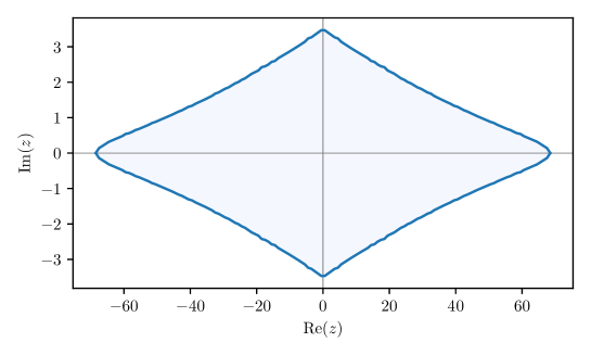
Figure 1. Region where the Taylor series theoretically is faster than the Stirling series, counting only arithmetic operations in argument reduction and polynomial evaluation (here for $p=1000$). Observe that the scale of the imaginary axis is exaggerated in this visualization.

Asymptotically, the Taylor series should be faster than the Stirling series inside a narrow diamond-shaped region (see Figure 1) whose boundaries grow with the precision $p$.

We have not attempted to determine a formula for the asymptotic shape of this region. In practice, the scale and shape of the boundary will be different from a theoretical prediction due to elementary function costs, non-constant costs of arithmetic operations, differences in working precision, etc., and suitable regions for using the Taylor series must be determined empirically.

5.2. McCullagh’s series

Differentiating the Taylor series (63) allows computing $[1/\Gamma(z)]^{\prime}$ about as rapidly as $1/\Gamma(z)$, and with two Taylor series evaluations, we can recover $\Gamma^{\prime}(z)$ or $\psi(z)$.

An alternative expansion for $\psi(z)$ is McCullagh’s series [McC81] [Bee17, Section 18.2.7]

$$\psi(1+z)=-\gamma-\sum_{n=1}^{\infty}(-z)^{n}\left(d_{n}+\frac{c_{n}}{z+n}\right),$$ (74)

where the coefficients

$$c_{n}=\frac{1}{n^{n}},\;d_{n}=\sum_{k=n+1}^{\infty}\frac{1}{k^{n+1}}=\zeta(n+1,n+1).$$ (75)

can be precomputed. This series converges even more quickly than the Taylor series for $1/\Gamma(z)$, having terms of order $|z|^{n}n^{-n}$, though it requires more work per term.

McCullagh’s series can also be differentiated to obtain expansions of $\psi^{(k)}(z)$. Integrating term by term yields the rapidly convergent

$$\log\Gamma(1+z) =-\gamma z+\sum_{n=1}^{\infty}\frac{(-z)^{n+1}}{n+1}\left(d_{n}+\frac{c_{n}}{n}{}_{2}F_{1}\!\left(1,n+1;\,n+2;\,-\frac{z}{n}\right)\right)$$ (76)

$$=-\gamma z+\sum_{n=1}^{\infty}\left[\frac{(-z)^{n+1}d_{n}}{n+1}-\log\left(1+\frac{z}{n}\right)-\sum_{k=1}^{n}\frac{(-z)^{k}}{kn^{k}}\right]$$ (77)

which however is less suitable for computations since there does not seem to be a simple recurrence relation for the logarithmic (${}_{2}F_{1}$ function) terms.

5.3. Chebyshev and minimax polynomials

Taylor polynomials minimize error near the expansion point, but Chebyshev or minimax approximations give better accuracy uniformly on an interval.

Table 5. Maximum absolute error (estimated) of degree-$D$ polynomial approximations of $1/\Gamma(x)$ on short real intervals.

$D$	Taylor, $[0.5,1.5]$	Taylor, $[0.75,1.25]$	Chebyshev, $[1,2]$	Minimax, $[1,2]$
$5$	$2.1\cdot 10^{-4}$	$2.8\cdot 10^{-6}$	$3.4\cdot 10^{-6}$	$3.8\cdot 10^{-7}$
$10$	$1.0\cdot 10^{-8}$	$4.9\cdot 10^{-12}$	$7.1\cdot 10^{-12}$	$5.9\cdot 10^{-13}$
$50$	$1.2\cdot 10^{-59}$	$5.0\cdot 10^{-75}$	$4.3\cdot 10^{-75}$
$100$	$2.0\cdot 10^{-139}$	$7.7\cdot 10^{-170}$	$6.3\cdot 10^{-170}$
$200$	$4.2\cdot 10^{-323}$	$1.3\cdot 10^{-383}$	$9.2\cdot 10^{-384}$
$500$	$2.8\cdot 10^{-964}$	$4.3\cdot 10^{-1115}$	$2.1\cdot 10^{-1117}$

True minimax polynomials are optimal by definition, but they are expensive to compute, which largely limits their usefulness to machine precision. Chebyshev interpolants, however, are easy to generate while being nearly as accurate as minimax polynomials of the same degree [Nat13, Section 3.11] [Tre19, Theorem 16.1].

For any $N$-times differentiable function $f$ on an interval $[a,b]$, let $f_{N}(x)$ be the degree-($N-1$) Lagrange interpolating polynomial of $f$ at the Chebyshev nodes

$$x_{k}=\frac{1}{2}(a+b)+\frac{1}{2}(b-a)\cos\!\left(\frac{2k-1}{2N}\pi\right),\quad 1\leq k\leq N.$$ (78)

Then the standard error bound

$$|f(x)-f_{N}(x)|\leq\frac{1}{2^{N-1}N!}\left(\frac{b-a}{2}\right)^{N}\max_{\xi\in[a,b]}|f^{(N)}(\xi)|,\quad x\in[a,b]$$ (79)

suggests that, for an interval of width $b-a=1$, Chebyshev interpolants will have worst-case error about $2^{-N}$ times that of Taylor polynomials of the same degree (in the worst case of radius $1/2$ for the Taylor series). The Taylor series will break even with the Chebyshev interpolant for the average input (radius $1/4$). Numerical values (Table 5) confirm this.

Chebyshev interpolants are thus clearly better if we want to achieve a fixed accuracy on a real interval. However, there are some points in favor of using the Taylor series:

• The Taylor series can easily be truncated according to the precision as well as the proximity to the expansion point, and will then perform nearly as well as the Chebyshev interpolant on average. In practice, input to the gamma function is not necessarily uniform: arguments close to integers often appear in perturbation problems, favoring the Taylor series.

• Computing the truncated Taylor series to length $N$ turns out to be somewhat cheaper than evaluating $1/\Gamma(x)$ at $N$ points. In fact, the most efficient way to construct Chebyshev interpolants for the reciprocal gamma function appears to be to compute Taylor polynomials and evaluate these.

• The Taylor series is better if we want to to extend the approximation on $[a,b]$ to complex arguments inside a box $[a,b]+[-c,c]i$. (On the other hand, if we want to optimize for such a box with large $c$, then a Chebyshev interpolant along the imaginary axis might be better.)

6. Hypergeometric methods

The methods discussed so far require $\widetilde{O}(p^{2})$ bit operations to compute $\Gamma(z)$ to $p$-bit accuracy assuming that $z$ is fixed. The methods that will be discussed next are interesting since they lead to improved asymptotic complexity bounds. The two main theorems on the complexity of gamma function computation are due, in respective order, to Brent [Bre76a] and Borwein [Bor87, BB87].

Theorem 6.1.

Let $z\not\in\{0,-1,-2,\ldots\}$ be a fixed algebraic number. Then $\Gamma(z)$ can be computed to $p$-bit accuracy using $O(M(p)\log^{2}p)=\widetilde{O}(p)$ bit operations.

Theorem 6.2.

Let $z\not\in\{0,-1,-2,\ldots\}$ be a fixed complex number. Then $\Gamma(z)$ can be computed to $p$-bit accuracy using $O(p^{1/2}\log^{2}p)$ arithmetic operations, or $\widetilde{O}(p^{3/2})$ bit operations (assuming that we can compute $z$ to $p$-bit accuracy at least this fast).

There are several alternative hypergeometric representations of the gamma function, any of which can be used to prove Theorems 6.1 and 6.2. All known series of this type converge at an ordinary geometric rate, requiring a number of terms proportional to $p$, and the subquadratic complexity simply results from exploiting the structure of hypergeometric terms. In fact, the constant-factor overheads are generally worse than those for the best global and local methods discussed earlier, and the subquadratic hypergeometric methods therefore only become competitive at extremely high precision (thousands of digits or more) where asymptotically fast arithmetic truly kicks in. One of our goals in this section will be to analyze constant factors to determine the most viable hypergeometric formulas.

We will generally assume that the argument of the gamma function is held fixed in order to analyze asymptotics with respect to the precision. For large enough $p$, the reduced-complexity hypergeometric methods should be faster than the Stirling series in some region around the origin (similar to Figure 1) whose boundaries grow with $p$, but we will not analyze the asymptotics of this region.

6.1. General techniques and error bounds

We recall that any hypergeometric series can be expressed in terms of the generalized hypergeometric function

$${}_{p}F_{q}(a_{1},\ldots,a_{p};b_{1},\ldots,b_{q};z)=\sum_{n=0}^{\infty}\frac{(a_{1})_{n}\dots(a_{p})_{n}}{(b_{1})_{n}\dots(b_{q})_{n}}\frac{z^{n}}{n!}.$$ (80)

If $p<q+1$ or if $p=q+1$ and $|z|<1$, the series converges at the same asymptotic rate as the sum of $z^{n}/(n!)^{q+1-p}$. Otherwise, it diverges at the rate of $z^{n}(n!)^{p-q-1}$ and must be interpreted in the sense of analytic continuation or asymptotic resummation. We will define the ${}_{2}F_{0}$ function via Kummer’s $U$-function as ${}_{2}F_{0}(a,b,z)=(-1/z)^{a}U(a,a-b+1,-1/z)$.

To keep things brief, we will analyze the asymptotic efficiency of most formulas below without giving explicit error bounds. Tail bounds for convergent series can be obtained easily by comparing with geometric series; see for example [Joh19a, Theorem 1], which also deals with parameter derivatives. Tail bounds for ${}_{2}F_{0}(a,b,z)$ valid for complex $a,b,z$ are given by Olver [Nat13, section 13.7] [Olv65]; in the special case of positive real $a,b$ and negative real $z$, the error is bounded by first omitted term.

The fast methods for evaluating hypergeometric series are generalizations of the methods for rising factorials discussed in section 2.4. Denoting the $n$th term in (80) by $t(n)$ and letting $r(n)=t(n)/t(n-1)$ denote the term ratio (a rational function of $n$), the $n$th partial sum can be written as a matrix product

$$\begin{pmatrix}r(n)&0\\ 1&1\end{pmatrix}\begin{pmatrix}r(n-1)&0\\ 1&1\end{pmatrix}\cdots\begin{pmatrix}r(1)&0\\ 1&1\end{pmatrix}=\begin{pmatrix}\prod_{k=0}^{n}r(k)&0\\ \sum_{k=0}^{n-1}\prod_{j=0}^{k}r(j)&1\end{pmatrix}.$$ (81)

This product can be computed using binary splitting (used in Theorem 6.1) or fast multipoint evaluation (used in Theorem 6.2); rectangular splitting is also viable [Joh14a], but does not improve the asymptotic bit complexity.

Hypergeometric sequences and functions should be understood as a special case of holonomic sequences and functions. A sequence is called holonomic if it satisfies a linear recurrence relation of order $r$ with rational function coefficients (a hypergeometric sequence has order $r=1$); the sum of an order-$r$ sequence can be evaluated as a product of size $(r+1)\times(r+1)$ matrices, using the same methods.

6.1.1. Derivatives

Any hypergeometric representation of the gamma function can be differentiated to yield representations of the digamma function $\psi(z)$ and higher derivatives. Indeed, for any fixed $n\geq 0$, Theorems 6.1 and 6.2 are valid with $\Gamma^{(n)}(z)$ or $\psi^{(n)}(z)$ instead of $\Gamma(z)$. The differentiated series are holonomic but not generally hypergeometric.

Explicit formulas for parameter derivatives of hypergeometric functions are typically not pretty, but as discussed in [Joh19a], an implementation can simply use the original formulas in combination with power series arithmetic. When power series arithmetic is combined with binary splitting this also leads to asymptotically fast algorithms for higher derivatives; in particular, the complexity is $\widetilde{O}(n^{2})$ for computing the first $n$ derivatives simultaneously to precision $p=\widetilde{O}(n)$.

Some of the following formulas have removable singularities at certain points; the appropriate limits can be computed in the same manner as derivatives.

6.2. Using incomplete gamma functions

One well-known method to compute the gamma function [Bre76a, Bre78, BB87] uses the decomposition

$$\Gamma(z)=\gamma(z,N)+\Gamma(z,N)$$ (82)

where

$$\gamma(z,N)=\int_{0}^{N}t^{z-1}e^{-t}dt,\quad\quad\Gamma(z,N)=\int_{N}^{\infty}t^{z-1}e^{-t}dt$$ (83)

are the lower and upper incomplete gamma functions (assuming $N>0$, $\operatorname{Re}(z)>0$). The free parameter $N$ may be taken to be an integer for efficient evaluation.

Since $\Gamma(z,N)\approx e^{-N}$, we have $\Gamma(z)\approx\gamma(z,N)$ to within $2^{-p}$ if $N\approx\log(2)p$.

The lower incomplete gamma function can be computed using

$$\gamma(z,N)\,=\,\frac{N^{z}e^{-N}}{z}{}_{1}F_{1}(1,z+1,N)\,=\,\frac{N^{z}e^{-N}}{z}\sum_{k=0}^{\infty}\frac{N^{k}}{(z+1)_{k}}.$$ (84)

If $N\approx\log(2)p$, then an asymptotic analysis using $(z+1)_{k}\approx k!\approx(k/e)^{k}$ shows that the total error in the approximation of $\Gamma(z)$ is of order $2^{-p}$ when the series is truncated after $e\log(2)p\approx 1.88417p$ terms.

The formula (82) becomes slightly more efficient if we compute $\Gamma(z,N)$ instead of neglecting this term, using the asymptotic expansion

$$\Gamma(z,N)\,=\,e^{-N}N^{z-1}{}_{2}F_{0}\left(1,1-z,-\tfrac{1}{N}\right)\,\sim\,e^{-N}N^{z-1}\sum_{k=0}^{\infty}\frac{(1-z)_{k}}{(-N)^{k}}.$$ (85)

Let $N=\alpha\log(2)\,p$ where $\alpha$ is a tuning parameter, which will be used to control the number of terms in $\eqref{eq:lowerseries}$ and $\eqref{eq:upperseries}$. Since $\eqref{eq:upperseries}$ is a divergent series, the accuracy that can be achieved is limited for any fixed $N$; we will need $\alpha\geq 0.5$ to ensure that we can reach an error of $2^{-p}$.

Suppose that $\eqref{eq:lowerseries}$ is truncated after $K$ terms and that $\eqref{eq:upperseries}$ is truncated after $L$ terms, and that the truncation errors are of the same order of magnitude as the $K$-th and $L$-th terms of the respective series. Then the errors $\varepsilon_{\gamma}$ and $\varepsilon_{\Gamma}$ for the respective terms in (82) are of order

$$\varepsilon_{\gamma}\approx e^{-N}\frac{N^{K}}{K!},\quad\varepsilon_{\Gamma}\approx e^{-N}\frac{L!}{N^{L}}.$$ (86)

We can solve $\varepsilon_{\gamma}=\varepsilon_{\Gamma}=2^{-p}$ asymptotically for $K$ and $L$ by substituting $k!\approx(k/e)^{k}$, taking logarithms, and employing the Lambert $W$ function. We obtain

$$K=\left(\frac{1-\alpha}{W_{0}\!\left(\frac{1-\alpha}{\alpha e}\right)}\right)\log(2)p,\quad L=\left(\frac{\alpha-1}{W_{-1}\!\left(\frac{\alpha-1}{\alpha e}\right)}\right)\log(2)p$$ (87)

where the $W_{-1}$ branch of the Lambert $W$ function is used for $L$ since we want the solution where the terms of the asymptotic series are decreasing and not increasing. The function $W_{-1}(x)$ is real for $-e^{-1}\leq x<0$; the lower inequality reflects the constraint $\alpha\geq 0.5$ required to achieve sufficient accuracy with the asymptotic series.

In the limit $\alpha\to 1$, we obtain $K=e\log(2)p\approx 1.88417p$ and $L=0$, minimizing the number of terms of the asymptotic series for $\Gamma(z,N)$.

In the limit $\alpha\to 0.5$, we obtain $K=p\log(2)/(2W(1/e))\approx 1.24459p$ and $L=p\log(2)/2\approx 0.346574p$. This minimizes the number of terms of the series of $\gamma(z,N)$. The total number of terms for both series is $K+L\approx 1.59116p$.

We can minimize the total number of terms $K+L$ numerically; the minimum occurs at $\alpha=\alpha_{0}\approx 0.546904$, where $K\approx 1.30970p$, $L\approx 0.179996p$ and $K+L\approx 1.48970p$. In practice, it is probably best to take a smaller $0.5<\alpha<\alpha_{0}$ since the series for $\gamma(z,N)$ must be computed with higher precision than that for $\Gamma(z,N)$ and thus requires more work for each term.

6.2.1. More points

The method using incomplete gamma functions amounts to computing the defining integral (1) using term-by-term integration of series expansions at $0$ and $\infty$. An idea is to expand the integrand at multiple points $0<t_{1}<\ldots<t_{n}<\infty$ using

$$(t+x)^{z-1}e^{-(t+x)}=t^{z-1}e^{-t}\sum_{n=0}^{\infty}{}_{1}F_{1}(-n,z-n,t){z-1\choose n}t^{-n}x^{n}$$ (88)

in which the series is holonomic. Unfortunately, this does not seem to lead to an improvement; the reduction in terms at $0$ and $\infty$ will not be significant unless we use vastly more terms in the middle.

6.3. Using Bessel functions

An alternative method uses the modified Bessel function $I_{\nu}$. We will need the convergent expansion

$$\Gamma(\nu+1)I_{\nu}(x)=\left(\frac{x}{2}\right)^{\nu}{}_{0}F_{1}\left(\nu+1,\frac{x^{2}}{4}\right)=\left(\frac{x}{2}\right)^{\nu}\sum_{k=0}^{\infty}\frac{1}{k!(\nu+1)_{k}}\left(\frac{x^{2}}{4}\right)^{k},$$ (89)

and the asymptotic expansion

$$I_{\nu}(x)=\frac{1}{\sqrt{2\pi x}}\left(e^{x}{}_{2}F_{0}\left(\tfrac{1}{2}+\nu,\tfrac{1}{2}-\nu,\tfrac{1}{2x}\right)-ie^{-x-\pi i\nu}{}_{2}F_{0}\left(\tfrac{1}{2}+\nu,\tfrac{1}{2}-\nu,-\tfrac{1}{2x}\right)\right)$$ (90)

valid at least for $x>0$. We obtain $\Gamma(z+1)$ if we choose a large enough $N$, compute $\Gamma(z+1)I_{z}(N)$ using (89) and $I_{z}(N)$ using (90), and divide.

Suppose that $\eqref{eq:besseliconvergent}$ is truncated after $K$ terms and that the series with prefactor $e^{x}$ in $\eqref{eq:besseliasymptotic}$ is truncated after $L$ terms, and that the truncation errors are of the same order of magnitude as the $K$-th and $L$-th terms of the respective series (we can ignore the ${}_{2}F_{0}$ series in $\eqref{eq:besseliasymptotic}$ with exponentially small prefactor). Then the relative errors $\varepsilon_{0}$ and $\varepsilon_{\infty}$ are of order

$$\varepsilon_{0}\approx\frac{e^{-N}}{(K!)^{2}}\left(\frac{N^{2}}{4}\right)^{K},\quad\varepsilon_{\infty}\approx\frac{L!}{(2N)^{L}}.$$ (91)

We assume that $N\approx\alpha\log(2)p$ for some tuning parameter $\alpha$. Solving asymptotically gives

$$K=\left(\frac{1-\alpha}{2W_{0}\!\left(\frac{1-\alpha}{\alpha e}\right)}\right)\log(2)p,\quad L=\left(-\frac{1}{W_{-1}\!\left(-\frac{1}{2\alpha e}\right)}\right)\log(2)p.$$ (92)

Real-valuedness of $W_{-1}(x)$ reflects the constraint $\alpha\geq 0.5$ required to achieve sufficient accuracy with the asymptotic series.

We can minimize $K$ by setting $\alpha=0.5$, giving $K\approx p\log(2)/(4W(1/e))\approx 0.622294p$ and $L\approx\log(2)p\approx 0.693147p$, with $K+L\approx 1.31544p$.

Minimizing $K+L$ gives $\alpha=\alpha_{0}\approx 0.639845$, with $K\approx 0.717353p$, $L\approx 0.369583p$ and $K+L\approx 1.08694p$. This is not necessarily the optimal strategy since the two series have somewhat different terms; a more realistic analysis should account for the relative costs of computing the terms of each series.

6.3.1. Alternative Bessel function algorithm

We can exploit the connection formula

$$I_{-\nu}=I_{\nu}+\frac{2\sin(\pi\nu)}{\pi}K_{\nu}(x).$$ (93)

involving the modified Bessel function of the second kind

$$K_{\nu}(x)=\left(\frac{2x}{\pi}\right)^{-1/2}e^{-x}{}_{2}F_{0}\left(\tfrac{1}{2}+\nu,\tfrac{1}{2}-\nu,-\tfrac{1}{2x}\right).$$ (94)

Let $A=\Gamma(z+1)I_{z}(N)$ and $B=\Gamma(-z+1)I_{-z}(N)$, both of which can be computed using (89). An application of the connection formula and the reflection formula for the gamma function gives

$$\Gamma(z)^{2}=\frac{A}{B}\frac{\pi}{z\sin(\pi z)}\left(1+\frac{2}{\pi\sin(\pi z)}\frac{K_{z}(N)}{I_{z}(N)}\right).$$ (95)

To compute $\Gamma(z)$, we can determine the correct sign of the square root from a low-precision approximation of $\Gamma(z)$ obtained by a different method (when $z>0$, we simply take the positive root).

We can choose $N\approx\tfrac{1}{2}\log(2)p$ so that $K_{z}(N)/I_{z}(N)\approx e^{-2N}$ is negligible, resulting in the approximation

$$\Gamma(z)\approx\pm\sqrt{\frac{A}{B}\frac{\pi}{z\sin(\pi z)}}.$$ (96)

In this case, we need $K\approx\tfrac{1}{2}e\log(2)p$ terms for each of the series $A$ and $B$, or $2K\approx e\log(2)p\approx 1.88417p$ terms in total. Bailey [Bai21] credits the “very efficient but little-known formula” (96) to Potter [Pot14] and reports using it in MPFUN package.

Alternatively, we can choose a somewhat smaller $N$ and compute $K_{z}(N)/I_{z}(N)$ using asymptotic expansions. Setting $N\approx\alpha\log(2)p$ and solving asymptotically for $e^{-2N}\frac{L!}{(2N)^{L}}=2^{-p}$ gives

$$K=\left(\frac{1-\alpha}{2W_{0}\!\left(\frac{1-\alpha}{\alpha e}\right)}\right)\log(2)p,\quad L=\left(\frac{2\alpha-1}{W_{-1}\!\left(\frac{2\alpha-1}{2\alpha e}\right)}\right)\log(2)p.$$ (97)

Because of the asymptotic series, we require $\alpha\geq 0.25$.

Minimizing $K$ gives $\alpha=0.25$ with $K\approx 3\log(2)p/(8W(3/e))\approx 0.430672p$ and $L\approx\tfrac{1}{2}\log(2)p\approx 0.346574p$, with $2K+2L\approx 1.55449$ terms in total.

Minimizing $K+L$ gives $\alpha\approx 0.358032$, where we need $2K+2L\approx 1.16604p$ terms in total. As noted previously, this is not necessarily the optimum in practice since the series have different terms and the asymptotic series require lower precision.

6.3.2. A third Bessel-type algorithm

Another interesting approximate formula is given by Smith [Smi06, eq. 94], here slightly rewritten:

$$\Gamma(z)^{2}\approx N^{2z}\left[-\frac{2(\gamma+\log(N))}{z}\,{}_{1}F_{2}(z,1,1+z,N^{2})+S_{z}(N)\right],$$ (98)

$$S_{z}(N)=\sum_{n=0}^{\infty}\frac{(-N)^{2n}}{n!^{2}}\left(\frac{1}{(z+n)^{2}}+\frac{2H_{n}}{n+z}\right),\quad H_{n}=\sum_{k=1}^{n}\frac{1}{k}.$$ (99)

The error is around $e^{-2N}$, though Smith does not provide a derivation of the formula or an error bound (we expect that this can be obtained by differentiating some Bessel function identity with respect to parameters). The function $S_{z}(N)$ is not hypergeometric, but it is holonomic. Smith’s formula appears to be less efficient than the other formulas considered above, but it hints that there may be a space of hypergeometric or holonomic approximation formulas for the gamma function that has not yet been fully explored.

6.4. Incomplete gamma versus Bessel

Which hypergeometric method is superior: the one using incomplete gamma functions or either algorithm using Bessel functions? The first Bessel function method requires the fewest terms, but the terms of the incomplete gamma functions are simpler. The winner may ultimately depend on implementation details.

For evaluating $\Gamma(z)$ with $z\in\mathbb{R}$ using the fast multipoint evaluation strategy ($\widetilde{O}(p^{3/2})$ complexity), the incomplete gamma function method runs around 30% faster than the Bessel function methods when implemented in Arb. For an empirical comparison between hypergeometric series and the Stirling series, see Section 7.

6.5. Products and quotients

Certain products and ratios of gamma functions can be evaluated without computing each gamma function separately. Smith [Smi06] gives a collection of formulas based on closed-form evaluations of the Gauss hypergeometric function ${}_{2}F_{1}(a,b;c;x)$ at fixed points $|x|<1$, where we need $-1/\log_{2}(|x|)$ terms per bit of precision. Notable examples include the beta function

$$B(a,b)=\frac{\Gamma(a)\Gamma(b)}{\Gamma(a+b)}=\frac{2}{2a+2b-1}\,\frac{{}_{2}F_{1}(1,2a+2b-1;\,a+b+\tfrac{1}{2};\,\tfrac{1}{2})}{{}_{2}F_{1}(2a-1,2b-1;\,a+b-\tfrac{1}{2};\,\tfrac{1}{2})},$$ (100)

the generalized reflection formula

$$\Gamma(M-z)\Gamma(M+z)=\frac{\sqrt{\pi}\,\Gamma(M+\tfrac{1}{2})}{{}_{2}F_{1}(2M-1-2z,2M-1+2z;\,2M-\tfrac{1}{2};\,\tfrac{1}{2})},$$ (101)

and the generalized shift (typo corrected)

$$\frac{\Gamma(z+S)}{\Gamma(z)}=\frac{1}{\sqrt{\pi}}\,\Gamma(S+\tfrac{1}{2})\,{}_{2}F_{1}(2z-1,2S;\,z+S;\,\tfrac{1}{2}).$$ (102)

Each of the above ${}_{2}F_{1}$ series requires 1 term per bit of precision. In the last two formulas, the gamma function values appearing as prefactors in the right-hand sides can be precomputed for fixed $M$ or $S$; elliptic integral identities (see below) can be used when $M+\tfrac{1}{2}$ or $S+\tfrac{1}{2}$ is a fraction $k/24$. Even more rapidly convergent series exist for the special shift $1/6$ [Smi06, Ekh04]:

$$\frac{\Gamma(z+\tfrac{1}{6})}{\Gamma(z)}=\frac{3\,\Gamma(\tfrac{2}{3})}{2\sqrt{3\pi}\sqrt[3]{2}}\left(\frac{16}{27}\right)^{z}{}_{2}F_{1}(\tfrac{1}{3}-2z,\tfrac{2}{3}-2z;\,1-z;\,-\tfrac{1}{8}),$$ (103)

$$\frac{\Gamma(z+\tfrac{1}{6})}{\Gamma(z)}=\frac{\Gamma(\tfrac{3}{4})}{\Gamma(\tfrac{7}{12})\sqrt{2}\sin(\tfrac{5\pi}{12})}(3-24\eta)^{1/4-z}{}_{2}F_{1}(\tfrac{1}{2}-2z,\tfrac{1}{2}-2z;\,1-z;\,\eta),$$ (104)

where $\eta=(2-\sqrt{3})/4\approx 0.0669873$.

Such formulas are potentially useful for evaluating the gamma function on a grid of equidistant points.

Smith proposes an algorithm for reducing the argument of $\Gamma(1+z)$ to the strip $0\leq\operatorname{Re}(z)\leq 1/48$ using generalized reflections or shifts (101, 102) and evaluation of elliptic integrals, or more generally to an arbitrarily small box $0\leq\operatorname{Re}(z)\leq 1/N$, $0\leq\operatorname{Im}(z)\leq 1/N$ with the help of a table of precomputed gamma function values. This can be used to improve convergence of methods such as Taylor series, but it is not clear whether it is worth the overhead over more direct algorithms.

6.6. Elliptic integrals and special values

The constants $\Gamma(k/24)$ can be expressed in terms of the complete elliptic integral

$$K(m)=\tfrac{1}{2}\pi\,{}_{2}F_{1}(\tfrac{1}{2},\tfrac{1}{2};\,1;\,m)$$ (105)

evaluated at fixed algebraic points [CS67, BZ92]. For example,

$$\Gamma(\tfrac{1}{2}) =[2K(0)]^{1/2}=\sqrt{\pi},$$ (106)

$$\Gamma(\tfrac{1}{3}) =2^{7/9}3^{-1/12}\pi^{1/3}[K(\tfrac{1}{2}-\tfrac{1}{4}\sqrt{3}))]^{1/3},$$ (107)

$$\Gamma(\tfrac{1}{4}) =2\pi^{1/4}[K(\tfrac{1}{2})]^{1/2}.$$ (108)

The $K(m)$ values can be evaluated using binary splitting. Alternatively, $K(m)$ can be expressed in terms of the arithmetic-geometric mean

$$\operatorname{agm}(a_{0},b_{0})=\lim_{n\to\infty}a_{n}=\lim_{n\to\infty}b_{n},\quad\left(a_{n+1},b_{n+1}\right)=\left(\tfrac{a_{n}+b_{n}}{2},\sqrt{a_{n}b_{n}}\right)$$ (109)

which converges to $p$-bit accuracy after only $O(\log p)$ iterations.

We have, for example,

$$\Gamma(\tfrac{1}{4})=\sqrt{\frac{(2\pi)^{3/2}}{\operatorname{agm}(1,\sqrt{2})}},$$ (110)

and for $\pi$, the Brent-Salamin algorithm

$$\pi=\Gamma(\tfrac{1}{2})^{2}=\frac{4(\operatorname{agm}(1,1/\sqrt{2}))^{2}}{1-\sum_{n=0}^{\infty}2^{n}(a_{n}-b_{n})^{2}}.$$ (111)

The arithmetic-geometric mean iteration has better arithmetic complexity than series evaluation, and better bit complexity by a factor $O(\log p)$. It is not necessarily faster than binary splitting in practice if the hypergeometric series have favorable constant factors. All recent record computations [Yee21] of $\pi=\Gamma(1/2)^{2}$ have used the Chudnovsky series [CC88]

$$\frac{1}{\pi}=12\sum_{n=0}^{\infty}\frac{(-1)^{n}(6n)!(13591409+545140134n)}{(3n)!(n!)^{3}640320^{3n+3/2}},$$ (112)

less elegantly written as a linear combination of two ${}_{3}F_{2}$ functions, which requires only $1/\log_{2}(640320^{3}/1728)\approx 0.0212$ terms per bit, i.e. adding more than 14 decimal digits per term.

In a similar vein, Brown [Bro09] has derived several rapidly convergent hypergeometric series for $\Gamma(1/3)$ and $\Gamma(1/4)$, including the elegant pair

$$[\Gamma(\tfrac{1}{4})]^{4} =\frac{32\pi^{3}}{\sqrt{33}}\,{}_{3}F_{2}\left(\tfrac{1}{2},\tfrac{1}{6},\tfrac{5}{6};\,1,1;\,\tfrac{8}{1331}\right),$$ (113)

$$[\Gamma(\tfrac{1}{3})]^{6} =\frac{12\pi^{4}}{\sqrt{10}}\,{}_{3}F_{2}\left(\tfrac{1}{2},\tfrac{1}{6},\tfrac{5}{6};\,1,1;\,-\tfrac{9}{64000}\right),$$ (114)

requiring only $0.136$ and $0.0782$ terms per bit, respectively. The formula (114) is used in Arb to compute $\Gamma(1/3)$ as it was found to be faster than the arithmetic-geometric mean.

Products of $\Gamma(x)$ evaluated at fixed rational $x$ can be algebraic numbers. Using such identities, Vidunas [Vid05] shows that any $\Gamma(k/n)$ where $n$ divides 24 or 60 can be expressed in terms of algebraic numbers, rational powers of $\pi$, and the set of numbers $\Gamma(x)$ with $x\in\{1/3,1/4,1/5,2/5,1/8,1/15,1/20,1/24,1/60,7/60\}$.

An alternative approach to numerical calculation of special gamma function values is to use the $q$-series of elliptic modular forms. For example,

$$\Gamma(\tfrac{1}{4})=\sqrt{2}\pi^{3/4}\theta(i)=\sqrt{2}\pi^{3/4}\vartheta(e^{-\pi})$$ (115)

in terms of the Jacobi theta function

$$\theta(\tau)=\vartheta(q)=1+2\sum_{n=1}^{\infty}q^{n^{2}},\quad q=e^{\pi i\tau}.$$ (116)

Using a simple recurrence relation for the powers of $q$, the theta series can be evaluated using $O(p^{1/2})$ arithmetic operations, which is better than the arithmetic complexity for hypergeometric series (though not as good as the arithmetic-geometric mean). This complexity can in fact be improved even further [EHJ18, NS17]. The bit complexity is unfortunately not quasilinear in $p$ (binary splitting is not useful here), but the implied constant factors are small. Using (115), in which $q\approx 0.0432$, we need only $0.470p^{1/2}$ terms for $p$-bit accuracy. We can accelerate the convergence further using modular transformations and special values of the elliptic lambda function [Yi04]; for example,

$$\Gamma(\tfrac{1}{4})=\pi^{3/4}\left[\frac{6\sqrt{5}\sqrt{1+\sqrt{5}}}{3+\sqrt{5}+\left(\sqrt{3}+\sqrt{5}+{60}^{1/4}\right){\left(2+\sqrt{3}\right)}^{1/3}}\right]\vartheta(e^{-45\pi})$$ (117)

where $e^{-45\pi}\approx 4\cdot 10^{-62}$, requiring $0.0701p^{1/2}$ terms. The first 128 terms of this theta series suffice to determine $\Gamma(1/4)$ to one million decimal digits.

6.7. The digamma function

The digamma function $\psi(z)$ can be computed by evaluating a formula for $\Gamma(z)$ using length-two power series arithmetic (dual numbers), but it is useful to have more direct formulas.

The best available method for Euler’s constant $-\psi(1)=\gamma$ is the Brent-McMillan algorithm [BM80] based on Bessel functions. It uses the formula

$$\gamma=\frac{S_{0}(2N)-K_{0}(2N)}{I_{0}(2N)}-\log(N)$$ (118)

where the right-hand side should be evaluated using binary splitting applied to the three series (the first of which is holonomic)

$$S_{0}(x)=\sum_{k=0}^{\infty}\frac{H_{k}}{(k!)^{2}}\left(\frac{x}{2}\right)^{2k},\quad I_{0}(x)=\sum_{k=0}^{\infty}\frac{1}{(k!)^{2}}\left(\frac{x}{2}\right)^{2k},$$ (119)

$$I_{0}(x)K_{0}(x)\sim\frac{1}{2x}\sum_{k=0}^{\infty}\frac{[(2k)!]^{3}}{(k!)^{4}8^{2k}x^{2k}}.$$ (120)

A convenient error bound is available: if the first two series are summed up to the $k=K-1$ term inclusive and the third series is summed up to $k=2K-1$ inclusive, where $K\geq\alpha N+1$, $\alpha=3/W_{0}(3/e)\approx 4.97063$, then the error in (118) is bounded by $24e^{-8N}$ [BJ15]. We need about $\tfrac{1}{2}\alpha\log(2)p\approx 1.72269p$ terms in total for $p$-bit accuracy. This actually overestimates the true cost because the first two series can share some of the computations and the third series only needs to be computed with $p/2$-bit precision.

Used in combination with recurrence relations and Gauss’s digamma theorem

$$\psi\!\left(\frac{k}{q}\right)=-\gamma-\log\!\left(2q\right)-\frac{\pi}{2}\cot\!\left(\frac{\pi k}{q}\right)+2\sum_{n=1}^{\left\lfloor\left(q-1\right)/2\right\rfloor}\cos\!\left(\frac{2\pi nk}{q}\right)\log\!\left(\sin\!\left(\frac{\pi n}{q}\right)\right)$$ (121)

($q\geq 2$, $1\leq k\leq q-1$), this also yields the most efficient method to compute $\psi(k/q)$ for any small integers $k,q$.

The digamma function of a general argument $z$ can be represented by means of the constant $\gamma$, elementary functions, and a single rapidly convergent hypergeometric series:

$$\psi(z)=-\gamma-\frac{1}{2z}-\frac{\pi\cot(\pi z)}{2}-z^{2}\left[\frac{(z^{2}-5)}{4(z^{2}-1)}\,{}_{8}F_{7}(a;b;-\tfrac{1}{4})\right]$$ (122)

where

$a=(1,1,1-z,1-z,1+z,1+z,2+\tfrac{z}{\sqrt{5}},2-\tfrac{z}{\sqrt{5}})$,

$b=(\tfrac{3}{2},2,2,2+z,2-z,1+\tfrac{z}{\sqrt{5}},1-\tfrac{z}{\sqrt{5}})$.

The terms of the ${}_{8}F_{7}$ series satisfy the recurrence relation

$$\frac{t(k)}{t(k-1)}=\frac{k(k^{2}-z^{2})^{2}(z^{2}-5(k+1)^{2})}{2(k+1)^{2}(2k+1)((k+1)^{2}-z^{2})(5k^{2}-z^{2})},$$ (123)

involving only rational numbers and $z^{2}$. At 0.5 terms per bit, the convergence is more rapid than for any of the known hypergeometric series for the gamma function, although the terms are more complicated.

The function in brackets in (122) is the ordinary generating function

$$\frac{z^{2}-5}{4(z^{2}-1)}{}_{8}F_{7}(a;b;-\tfrac{1}{4})=Z(z^{2});\quad Z(z)=\sum_{n=0}^{\infty}\zeta(2n+3)z^{n}.$$ (124)

of the odd integer zeta values $\zeta(3),\zeta(5),\ldots$. The hypergeometric series is given by Borwein, Bradley and Crandall ([BBC00], unnumbered equation between (62) and (63)) as

$$Z(z^{2})=\sum_{k=1}^{\infty}\frac{(-1)^{k+1}}{k^{3}{2k\choose k}}\left(\frac{1}{2}+\frac{2}{1-z^{2}/k^{2}}\right)\prod_{j=1}^{k-1}\left(1-\frac{z^{2}}{j^{2}}\right)$$ (125)

from which one can derive the closed ${}_{8}F_{7}$ form or the alternative representation

$$Z(z^{2}) =\frac{{}_{4}F_{3}(1,1,1-z,1+z;\,\tfrac{3}{2},2,2;\,-\tfrac{1}{4})}{4}$$ (126)

$$-\frac{{}_{3}F_{2}(1-z,1-z,1+z;\,\tfrac{3}{2},2-z;\,-\tfrac{1}{4})}{2z(z-1)}$$ (127)

$$-\frac{{}_{3}F_{2}(1-z,1+z,1+z;\,\tfrac{3}{2},2+z;\,-\tfrac{1}{4})}{2z(z+1)}.$$ (128)

Borwein, Bradley and Crandall use symbolic differentiation of (125) to derive binary splitting schemes for isolated integer zeta values. They seem to have overlooked (or neglected to mention) the fact that the same series can be used for asymptotically fast multi-evaluation of integer zeta values by using binary splitting together with power series arithmetic (this is more efficient than the incomplete gamma function method proposed in [BBC00]; see the discussion in [Joh14b]), as well as the fact that this series can be used for reduced-complexity evaluation of the general function values $\psi(z)$ and $\psi^{(m)}(z)$.

We have curiously not found any other hypergeometric representations of $\psi(z)$ in the literature apart from the well-known

$$\psi(z)=-\gamma+\left(z-1\right)\,{}_{3}F_{2}(1,1,2-z,2,2,1),\quad\operatorname{Re}(z)>0,$$ (129)

where the ${}_{3}F_{2}$ series converges too slowly to be usable for direct summation. A fast algorithm can be constructed from (129) by connecting the solutions at $x=0$ and $x=1$ of the differential equation defining ${}_{3}F_{2}(-;-;x)$, using the standard analytic continuation method [vdH99, Mez11] for holonomic functions. We do not attempt to construct an explicit algorithm here.

7. Implementation results and algorithm selection

We implemented the following algorithms in Arb (version 2.21) as part of a complete rewrite (some 10,000 new lines of C code) of the library’s functions for $\Gamma(z)$, $1/\Gamma(z)$ and $\log\Gamma(z)$ for real, complex and rational $z$:

• The Stirling series (together with Algorithm 6).

• Hypergeometric series (using the incomplete gamma function method with the combined ${}_{1}F_{1}$ and ${}_{2}F_{0}$ series).

  • Fast multipoint evaluation for generic arguments.

  • Binary splitting for rational arguments.

• The Taylor series.

• Factorials and elliptic integrals in special cases.

The algorithms are available as separate functions; the user-facing functions (arb_gamma, etc.) try to choose the best algorithm automatically.

The previous version mainly used a less optimized implementation of the Stirling series together with factorials and elliptic integrals for special cases. We also implemented other algorithms (Spouge’s formula, Bessel function formulas) for timing comparisons, but did not include them in the library after experiments clearly showed worse performance.

7.1. Varying precision

Table 6 and Figure 2 show the performance of different algorithms when the argument is a fixed small real number, for a varying precision $p$ (we display the number of decimals $d$, equivalent to binary precision $p=\log_{2}(10)d$).

Table 6. Time (in seconds) to compute $\Gamma(x)$, $x\approx 1.3$, to $d$ decimal digits using different algorithms: Spouge’s formula (“first” including cost of generating coefficients, “repeated” with coefficients cached), the Stirling series, Taylor series, hypergeometric series (using fast multipoint evaluation). Lower table: using hypergeometric series with binary splitting, with $x=13/10$ given as an exact rational number.

$d$	Spouge	Spouge	Stirling	Stirling	Taylor	Taylor	Hyper-
	(first)	(repeated)	(first)	(repeated)	(first)	(repeated)	geometric
$10$	$2.2\cdot 10^{-5}$	$4.6\cdot 10^{-6}$	$5.2\cdot 10^{-6}$	$4.1\cdot 10^{-6}$	$3.3\cdot 10^{-5}$	$2.6\cdot 10^{-7}$	$4.7\cdot 10^{-5}$
$30$	$6.1\cdot 10^{-5}$	$1.2\cdot 10^{-5}$	$1.3\cdot 10^{-5}$	$8.8\cdot 10^{-6}$	$9.6\cdot 10^{-5}$	$1.8\cdot 10^{-6}$	$0.00012$
$100$	$0.00035$	$5.2\cdot 10^{-5}$	$5.2\cdot 10^{-5}$	$2.9\cdot 10^{-5}$	$0.00082$	$8.6\cdot 10^{-6}$	$0.00032$
$300$	$0.0021$	$0.00025$	$0.00038$	$9.6\cdot 10^{-5}$	$0.0077$	$4.0\cdot 10^{-5}$	$0.0011$
$1000$	$0.029$	$0.0027$	$0.0021$	$0.00073$	$0.13$	$0.00046$	$0.0064$
$3000$	$0.47$	$0.042$	$0.015$	$0.0064$	$1.7$	$0.0051$	$0.11$
$10000$	$11$	$1.0$	$0.20$	$0.087$	$40$	$0.082$	$0.95$
$30000$	$184$	$16$	$2.3$	$1.0$	$807$	$1.0$	$7.1$
$100000$	$3683$	$266$	$38$	$16$			$67$
$300000$			$478$	$173$			$481$
$1000000$							$4108$

Hypergeometric (rational $x=13/10$, binary splitting)
$d$		$d$		$d$
$10$	$1.8\cdot 10^{-5}$	$1000$	$0.0012$	$100000$	$0.49$
$30$	$3.4\cdot 10^{-5}$	$3000$	$0.0045$	$300000$	$2.0$
$100$	$9.7\cdot 10^{-5}$	$10000$	$0.021$	$1000000$	$7.9$
$300$	$0.00030$	$30000$	$0.096$	$3000000$	$31$

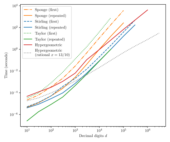
Figure 2. Time (in seconds) to compute $\Gamma(x)$, $x\approx 1.3$, to $d$ decimal digits using different algorithms (see Table 6).

7.1.1. Quadratic algorithms

Spouge’s formula, the Stirling series and the Taylor series all have complexity $\widetilde{O}(p^{2})$ with and without precomputation, but with different amounts of overhead. These trends are clearly visible in Figure 2.

The Taylor series is the fastest method up to perhaps $10^{4}$ decimal digits assuming that coefficients are precomputed. The speedup over the Stirling series is roughly $15\times$ at 10 digits, $3.5\times$ at 100 digits, and $1.5\times$ at 1000 digits. These figures are only rough estimates, and vary with the argument. (The input represents a near-worst case for the Stirling series, which performs better with larger $|z|$; more on this below.) In theory, the Taylor series should be $O(\log p)$ faster than the Stirling series asymptotically, but this is not seen in practice.

The Taylor series has the slowest precomputation. The precomputation time for 1000-digit precision would be roughly 0.1 seconds, which is an unacceptably large overhead for a first call to the gamma function. In the final implementation used in the library, we decided not to compute Taylor coefficients at runtime. Instead, we include a static 130 KB table of Taylor coefficients ($N=536$, $p=3456$), supporting precision up to around 1000 digits; we simply avoid the Taylor series at higher precision where the speedup over the Stirling series in any case would be small. The size of this table is about half the total size of tables used for elementary functions [Joh15], or 5% of the library binary size.

Spouge’s formula is, as expected, significantly slower than the Stirling series. A more optimized implementation could perhaps save a factor two, but this would not affect the conclusion.

The most interesting result is the low precomputation cost for the Stirling series thanks to the fast Bernoulli number generation (Algorithm 5) in combination with the improved Stirling series (Algorithm 6). Some authors have argued that the Bernoulli numbers in the Stirling series are “inconvenient” [Smi06], and in many earlier implementations, a first call to the gamma function has indeed been 10 or 100 times slower than subsequent calls [Lau05, Joh14a]. This is no longer the case: generating Bernoulli numbers now only costs the equivalent of 1-2 extra evaluations of the gamma function. What is notable is that we have achieved this without sacrificing performance for repeated evaluations, which would be the tradeoff if we simply were to choose a very large (suboptimal) $\beta=r/p$.

Subquadratic algorithms

Binary splitting evaluation of hypergeometric series is highly efficient for rational arguments, outperforming the Stirling and Taylor series from about 2000 digits. Figure 2 clearly shows the $\widetilde{O}(p)$ complexity.

The subquadratic ($\widetilde{O}(p^{3/2})$) complexity for generic $z$ with the hypergeometric method is also visible in Figure 2, but it only breaks even with Stirling series at extremely high precision: around $10^{6}$ bits if Bernoulli numbers have not been cached, and at around $10^{6}$ digits ($p\approx 3\cdot 10^{6}$) with Bernoulli numbers cached.

The high crossover with cached Bernoulli numbers reaffirms the benchmark results in [Joh14a], but that study found a much lower crossover around $p$ = 30,000 for a first evaluation when Bernoulli numbers are not cached. This large improvement for the initial call to the Stirling series is due to the use of Algorithm 6.

Coincidentally, the crossover points are right around the range where storing Bernoulli numbers in memory starts to become an issue on a typical 2021-era laptop. For example, with Algorithm 6, we need 10 GB of Bernoulli numbers to use the Stirling series for 600,000 digits of precision. To use the Stirling series at higher precision, it might be better to avoid caching Bernoulli numbers and accept a factor 2-3 slowdown.

We did not optimize the hypergeometric series evaluation at lower precision. Using rectangular splitting instead of fast multipoint evaluation should make the method more competitive with the quadratic algorithms for $p<10^{4}$ [Joh14a].

7.2. Varying argument

When the variable $z$ as well as the precision $p$ are allowed to vary, finding optimal cutoffs between several algorithms is complicated.

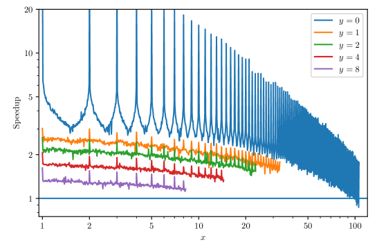
Figure 3. Speedup using the Taylor series instead of the Stirling series to compute $\Gamma(x+yi)$, here at precision $p=333$ (100 decimal digits). The graphs end at the point where the default gamma function algorithm in Arb switches from the Taylor series to the Stirling series. The axes of the figure are logarithmic.

For switching between the Taylor series and the Stirling series, we implemented experimentally-determined heuristics:

• If $z$ is real, let $r=\lfloor z+1/2\rfloor$. If $p<40$ or if the radius of the ball for $z$ is greater than $2^{-16}$, we use the Taylor series if $|r|<160$. Otherwise, we use the Taylor series if $-40-(p-40)/4<r<70+(p-40)/8$.

• If $z$ is complex with $x=|\operatorname{Re}(z)|$, $y=|\operatorname{Im}(z)|$, we do not use the Taylor series if either $p<128$ and $y>4$, $p<256$ and $y>5$, $p<512$ and $y>8$, $p<1024$ and $y>9$, or $y>10$. If all these checks pass, we use the Taylor series if $x(1.0+0.75y)>8+0.15p$.

• In all cases, we still fall back on the Stirling series if $p$ or $|z|$ are too large to achieve $p$-bit accuracy with the available precomputed Taylor coefficients (this is checked by computing the required working precision and number of terms and inspecting the table of coefficients).

Figure 3 demonstrates the speedup over the Stirling series and the cutoffs for $p=333$. We can see that the Taylor series performs better near integers and gradually performs worse with increased $x$ and $y$. The cutoffs are not quite optimal: we sometimes avoid the Taylor series even where it would yield a $2\times$ speedup. Overall, however, the tuning is reasonable, and we never use the Taylor series where it would be more than a few percent slower than the Stirling series.

We have also implemented experimentally-determined cutoffs for choosing algorithms (Taylor series, the Stirling series, elliptic integrals, hypergeometric series, factorials) to compute $\Gamma(x)$ with rational $x=k/q$, where we must account for the magnitude $|x|$ as well as the size of the denominator $q$. We omit the details.

7.3. Previous implementations

Compared to the previous implementation of the gamma function in Arb, the greatest speedup (typically a factor 2 to 10) is observed where the Taylor series is used for small real or complex variables.

Where the Taylor series is not used, our improvements to the Stirling series often yields a factor 1.5 to 2 speedup over the previous version except for large arguments at low precision, where the performance is unchanged. For the first call (requiring Bernoulli numbers to be computed), the speedup can be more than a factor 10.

With these improvements, the gamma function in Arb is typically 5-6 times faster than either Pari/GP 2.13 [The21b] (real and complex variables) or MPFR 4.1.0 [FHL⁺07] (real variables). The speedup is greater at low precision (more than a factor 10 at machine precision) and for a first call to the gamma function (at 10,000 digits, Arb is 1000 times faster than MPFR).

8. Open problems

We conclude with a collection of interesting problems for future research.

Open problem 8.1.

What are tight bounds for the error terms in the Lanczos and Spouge formulas (and other formulas of this type)? What are tight bounds for the error in the Stieltjes continued fraction? Can there be a unified theory for global approximations of the gamma function that subsumes ad-hoc developments? We note that Pugh [Pug04, Chapter 11] gives some more specific unsolved problems relating to the Lanczos approximation.

Open problem 8.2.

Is it possible to re-expand the remainder term $R_{N}(z)$ in the Stirling series in a way that reduces the computational complexity?

Open problem 8.3.

Is $\widetilde{O}(p^{3/2})$ the best possible complexity for computing the gamma function to $p$-bit accuracy at a generic point? Is there an algorithm with quasilinear complexity?

Open problem 8.4.

What is the complexity of computing $\Gamma(z)$ or $\Gamma^{*}(z)$ to $p$-bit accuracy accounting for both $p$ and the value $z$? Is it possible to achieve subquadratic complexity with respect to $p$ uniformly in $z$?

Open problem 8.5.

In realistic computational complexity models, what are the precise boundaries (as functions of both $p$ and $z$) for optimal selection between the Taylor series, the Stirling series, and other algorithms?

Open problem 8.6.

In what ways can $\Gamma(z)$ and $\psi(z)$ be expressed in terms of hypergeometric or holonomic functions with $z$ as a parameter? For example, is it possible to express $\Gamma(z)$ itself strictly in terms of hypergeometric functions ${}_{p}F_{q}(\{a_{j}\};\{b_{j}\};x)$ where the parameters $\{a_{j}\}$, $\{b_{j}\}$ are fixed rational functions of $z$ and where $x$ is a fixed point strictly within the radius of convergence of the ${}_{p}F_{q}$ series? Are the known formulas for $\Gamma(z)$ and $\psi(z)$ the most efficient possible?

Open problem 8.7.

Are there any rapidly convergent hypergeometric series or arithmetic-geometric mean type formulas for $\Gamma(z)$ at specialized algebraic points $z$ other than rationals with denominators 24? For example, can there be a formula similar to (114) for $\Gamma(1/5)$ or $\Gamma(\sqrt{-3})$? This would seemingly require entirely different mathematical theory than the classical theory of elliptic integrals and elliptic modular forms.

Open problem 8.8.

Is it possible to generate efficient and formally verified code for the gamma function automatically? Generating useful code from first principles (e.g. with only the defining integral (1) given as input) seems to require symbolic knowledge about complex analysis and numerical techniques far beyond the capabilities of current tools for automated theorem proving and code generation. Current code generators for mathematical functions [KL14, LM15] typically require a bounded domain and a function satisfying a nice differential equation, and cannot be used for global computation of complex functions with essential singularities.

Open problem 8.9.

What are the worst cases for Ziv’s algorithm to ensure correct rounding in different precision formats?

Bounding a priori the precision required to ensure $p$-bit correct rounding of transcendental functions is a hard theoretical problem. Currently, the only solution is to perform an exhaustive search for worst-case input for a fixed $p$, which in turn reduces to a Diophantine approximation problem. Brisebarre and Hanrot [BH21] discuss state of the art methods for this problem and consider the feasibility of finding worst cases for rounding $\Gamma(x)$ on the interval $[1,2)$ with $p=113$.

Open problem 8.10.

To ensure that Ziv’s strategy terminates, we need to be able to check for representable (e.g. algebraic) points $z$ where $\Gamma(z)$ is exactly representable. For example, in real binary floating-point arithmetic, we need to detect $z\in\mathbb{Z}[\tfrac{1}{2}]$ for which $\Gamma(z)\in\mathbb{Z}[\tfrac{1}{2}]$. Conjecturally, the only points of this kind are trivial, i.e. the positive integers. This conjecture can be generalized to the following questions:

• Are $\Gamma(z)$ and $\log\Gamma(z)$ transcendental for all $z\in\overline{\mathbb{Q}}\setminus\mathbb{Z}$?

• Are $\psi(z)$, $\psi^{(n)}(z)$ and $\Gamma^{(n)}(z)$ $(n\geq 1)$ transcendental for all $z\in\overline{\mathbb{Q}}\setminus\mathbb{Z}_{\leq 0}$?

Currently, $\Gamma(z)$ is known to be transcendental for rational arguments $k+\tfrac{1}{2}$, $k+\tfrac{1}{3}$, $k+\tfrac{1}{4}$ and $k+\tfrac{1}{6}$ [Wal06]. The special case of establishing the irrationality (and transcendence) of $-\psi(1)=\gamma$ is of course famously open.

9. Acknowledgements

The author thanks Daniel Schultz for complaining that the gamma function in Arb was slow, which ultimately led us down this rabbit hole.

Karim Belabas pointed out a small improvement in Algorithm 5 over the original implementation in Arb. Problem 8.8 is inspired by a question posed by Jacques Carette.

The author was supported in part by the ANR grant ANR-20-CE48-0014-02 NuSCAP.

References

- [AS64] M. Abramowitz and I. A. Stegun, Handbook of mathematical functions with formulas, graphs, and mathematical tables, Dover, New York, 1964.
- [Bai21] David H. Bailey, MPFUN2020: A new thread-safe arbitrary precision package, https://www.davidhbailey.com/dhbpapers/mpfun2020.pdf, 2021.
- [BB87] J. M. Borwein and P. B. Borwein, Pi and the AGM, vol. 23, Wiley, New York, 1987.
- [BBC00] J. M. Borwein, D. M. Bradley, and R. E. Crandall, Computational strategies for the Riemann zeta function, Journal of Computational and Applied Mathematics 121 (2000), 247–296.
- [BC18] Jonathan M. Borwein and Robert M. Corless, Gamma and factorial in the monthly, The American Mathematical Monthly 125 (2018), no. 5, 400–424.
- [BCH11] J. C. A. Barata, L. F. Canto, and M. S. Hussein, New asymptotic formulae for the point Coulomb phase shift, Brazilian Journal of Physics 41 (2011), no. 1, 50–58.
- [Bee17] Nelson HF Beebe, The mathematical-function computation handbook, Springer, 2017.
- [BGS07] A. Bostan, P. Gaudry, and É. Schost, Linear recurrences with polynomial coefficients and application to integer factorization and Cartier-Manin operator, SIAM Journal on Computing 36 (2007), no. 6, 1777–1806.
- [BH13] Richard P. Brent and David Harvey, Fast computation of Bernoulli, tangent and secant numbers, Computational and Analytical Mathematics, Springer New York, 2013, pp. 127–142.
- [BH21] Nicolas Brisebarre and Guillaume Hanrot, Integer points close to a transcendental curve and correctly-rounded evaluation of a function, working paper or preprint, May 2021.
- [Bin39] Jacques Philippe Marie Binet, Mémoire sur les intégrales définies eulériennes et sur leur application à la théorie des suites ainsi qu’à l’évaluation des fonctions des grands nombres, Journal de l’École Polytechnique (1839), no. XVI, 123–343.
- [BJ15] R. P. Brent and F. Johansson, A bound for the error term in the Brent-McMillan algorithm, Mathematics of Computation 84 (2015), no. 295, 2351–2359.
- [BK78] R. P. Brent and H. T. Kung, Fast algorithms for manipulating formal power series, Journal of the ACM 25 (1978), no. 4, 581–595.
- [Bla16] Iaroslav V. Blagouchine, Two series expansions for the logarithm of the gamma function involving stirling numbers and containing only rational coefficients for certain arguments related to , Journal of Mathematical Analysis and Applications 442 (2016), no. 2, 404–434.
- [Blo09] Remco Bloemen, Even faster calculation!, https://xn--2-umb.com/09/11/even-faster-zeta-calculation/, 2009.
- [BM80] R. P. Brent and E. M. McMillan, Some new algorithms for high-precision computation of Euler’s constant, Mathematics of Computation 34 (1980), no. 149, 305–312.
- [Bor85] Peter B Borwein, On the complexity of calculating factorials, Journal of Algorithms 6 (1985), no. 3, 376–380.
- [Bor87] P. B. Borwein, Reduced complexity evaluation of hypergeometric functions, Journal of Approximation Theory 50 (1987), no. 3, 193–199.
- [Bou83] L. Bourguet, Sur les intégrales eulériennes et quelques autres fonctions uniformes, Acta Mathematica 2 (1883), no. 0, 261–295.
- [Boy94] W. G. C Boyd, Gamma function asymptotics by an extension of the method of steepest descents, Proceedings of the Royal Society of London. Series A: Mathematical and Physical Sciences 447 (1994), no. 1931, 609–630.
- [BPZ07] Richard Brent, Colin Percival, and Paul Zimmermann, Error bounds on complex floating-point multiplication, Mathematics of Computation 76 (2007), no. 259, 1469–1481.
- [Bre76a] Richard P. Brent, Fast multiple-precision evaluation of elementary functions, Journal of the ACM 23 (1976), no. 2, 242–251.
- [Bre76b] Richard P Brent, Multiple-precision zero-finding methods and the complexity of elementary function evaluation, Analytic computational complexity, Elsevier, 1976, pp. 151–176.
- [Bre78] Richard P. Brent, A Fortran multiple-precision arithmetic package, ACM Transactions on Mathematical Software 4 (1978), no. 1, 57–70.
- [Bre18] by same author, On the accuracy of asymptotic approximations to the log-Gamma and Riemann-Siegel theta functions, Journal of the Australian Mathematical Society 107 (2018), no. 3, 319–337.
- [Bro09] C. H. Brown, An algorithm for the derivation of rapidly converging infinite series for universal mathematical constants, http://www.iamned.com/math/, 2009.
- [BS62] Heinrich Behnke and Friedrich Sommer, Theorie der analytischen Funktionen einer komplexen Veränderlichen, Springer-Verlag, 1962.
- [BZ92] J. M. Borwein and I. J. Zucker, Fast evaluation of the gamma function for small rational fractions using complete elliptic integrals of the first kind, IMA Journal of Numerical Analysis 12 (1992), 519–526.
- [BZ11] R. P. Brent and P. Zimmermann, Modern Computer Arithmetic, Cambridge University Press, 2011.
- [Cau21] Matthew F Causley, The gamma function via interpolation, https://arxiv.org/abs/2104.00697, 2021.
- [CC88] D. V. Chudnovsky and G. V. Chudnovsky, Approximations and complex multiplication according to Ramanujan, Ramanujan Revisited, Academic Press, 1988, pp. 375–472.
- [CGH+96] R. M. Corless, G. H. Gonnet, D. E. G. Hare, D. J. Jeffrey, and D. E. Knuth, On the Lambert W function, Advances in Computational Mathematics 5 (1996), no. 1, 329–359.
- [CH67] W. J. Cody and K. E. Hillstrom, Chebyshev approximations for the natural logarithm of the gamma function, Mathematics of Computation 21 (1967), no. 98, 198–198.
- [CH72] S. Chowla and P. Hartung, An “exact” formula for the m-th Bernoulli number, Acta Arithmetica 22 (1972), no. 1, 113–115.
- [Cha80] Bruce W. Char, On Stieltjes’ continued fraction for the gamma function, Mathematics of Computation 34 (1980), no. 150, 547–547.
- [Che16] Chao-Ping Chen, A more accurate approximation for the gamma function, Journal of Number Theory 164 (2016), 417–428.
- [Cod91] W. J. Cody, Performance evaluation of programs related to the real gamma function, ACM Transactions on Mathematical Software 17 (1991), no. 1, 46–54.
- [Cod93] by same author, Algorithm 715: SPECFUN–a portable FORTRAN package of special function routines and test drivers, ACM Transactions on Mathematical Software 19 (1993), no. 1, 22–30.
- [CPV+08] Annie AM Cuyt, Vigdis Petersen, Brigitte Verdonk, Haakon Waadeland, and William B Jones, Handbook of continued fractions for special functions, Springer, 2008.
- [CS67] Sarvadaman Chowla and Atle Selberg, On Epstein’s Zeta-function., Journal für die reine und angewandte Mathematik 1967 (1967), no. 227, 86–110.
- [CS19a] João R. Cardoso and Amir Sadeghi, Computation of matrix gamma function, BIT Numerical Mathematics 59 (2019), no. 2, 343–370.
- [CS19b] Robert M. Corless and Leili Rafiee Sevyeri, Stirling’s original asymptotic series from a formula like one of Binet’s and its evaluation by sequence acceleration, Experimental Mathematics (2019), 1–8.
- [Dav59] Philip J. Davis, Leonhard Euler’s integral: A historical profile of the gamma function: In memoriam: Milton Abramowitz, The American Mathematical Monthly 66 (1959), no. 10, 849.
- [EHJ18] Andreas Enge, William Hart, and Fredrik Johansson, Short addition sequences for theta functions, Journal of Integer Sequences 21 (2018), no. 2, 3.
- [Ekh04] Shalosh B. Ekhad, Forty “strange” computer-discovered [and computer-proved (of course!)] hypergeometric series evaluations, Personal Journal of Shalosh B. Ekhad and Doron Zeilberger, https://sites.math.rutgers.edu/~zeilberg/mamarim/mamarimhtml/strange.html (2004).
- [FA17] Lazhar Fekih-Ahmed, On the power series expansion of the reciprocal gamma function, https://arxiv.org/abs/1407.5983, 2017.
- [FHL+07] Laurent Fousse, Guillaume Hanrot, Vincent Lefèvre, Patrick Pélissier, and Paul Zimmermann, MPFR: A multiple-precision binary floating-point library with correct rounding, ACM Transactions on Mathematical Software 33 (2007), no. 2, 13:1–13:15.
- [Fil92] S. Fillebrown, Faster computation of Bernoulli numbers, Journal of Algorithms 13 (1992), no. 3, 431–445.
- [FLI21] FLINT developers, FLINT: Fast Library for Number Theory, 2021, Version 2.8.0, http://flintlib.org.
- [FS67] Antonino Machado Souza Filho and Georges Schwachheim, Algorithm 309: Gamma function with arbitrary precision, Communications of the ACM 10 (1967), no. 8, 511–512.
- [FW80] Arne Fransén and Staffan Wrigge, High-precision values of the gamma function and of some related coefficients, Mathematics of Computation 34 (1980), no. 150, 553–553.
- [GST07] Amparo Gil, Javier Segura, and Nico M Temme, Numerical methods for special functions, SIAM, 2007.
- [Har97] D.E.G Hare, Computing the principal branch of log-gamma, Journal of Algorithms 25 (1997), no. 2, 221–236.
- [Har10] David Harvey, A multimodular algorithm for computing Bernoulli numbers, Mathematics of Computation 79 (2010), no. 272, 2361–2361.
- [Has55] Cecil Hastings, Approximations for digital computers, Princeton University Press, 1955.
- [Höl86] Otto Hölder, Ueber die Eigenschaft der Gammafunction keiner algebraischen Differentialgleichung zu genügen, Mathematische Annalen 28 (1886), no. 1, 1–13.
- [HvdH21] David Harvey and Joris van der Hoeven, Integer multiplication in time ), Annals of Mathematics 193 (2021), no. 2, 563.
- [JE09] Eugen Jahnke and Fritz Emde, Funktionentafeln mit Formeln und Kurven, vol. 5, BG Teubner, 1909.
- [Joh14a] F. Johansson, Evaluating parametric holonomic sequences using rectangular splitting, Proceedings of the 39th International Symposium on Symbolic and Algebraic Computation, ISSAC ’14, ACM, 2014, pp. 256–263.
- [Joh14b] by same author, Fast and rigorous computation of special functions to high precision, Ph.D. thesis, RISC, Johannes Kepler University, Linz, 2014, http://fredrikj.net/thesis/.
- [Joh15] by same author, Efficient implementation of elementary functions in the medium-precision range, 22nd IEEE Symposium on Computer Arithmetic, ARITH22, 2015, pp. 83–89.
- [Joh17] Fredrik Johansson, Arb: Efficient arbitrary-precision midpoint-radius interval arithmetic, IEEE Transactions on Computers 66 (2017), no. 8, 1281–1292.
- [Joh19a] by same author, Computing hypergeometric functions rigorously, ACM Transactions on Mathematical Software 45 (2019), no. 3, 1–26.
- [Joh19b] by same author, Faster arbitrary-precision dot product and matrix multiplication, 2019 IEEE 26th Symposium on Computer Arithmetic (ARITH), IEEE, June 2019.
- [KL14] Olga Kupriianova and Christoph Lauter, Metalibm: A mathematical functions code generator, International Congress on Mathematical Software, Springer, 2014, pp. 713–717.
- [KL16] Tanya Khovanova and Joel Brewster Lewis, Skyscraper numbers, Journal of Integer Sequences 16 (2016), no. 13.7.2.
- [Köl72] K.S. Kölbig, Programs for computing the logarithm of the gamma function, and the digamma function, for complex argument, Computer Physics Communications 4 (1972), no. 2, 221–226.
- [Kuk72] Hirondo Kuki, Complex gamma function with error control, Communications of the ACM 15 (1972), no. 4, 262–267.
- [KZ08] S. Köhler and M. Ziegler, On the stability of fast polynomial arithmetic, Proceedings of the 8th Conference on Real Numbers and Computers (Santiago de Compostela, Spain), 2008.
- [Lan64] C. Lanczos, A precision approximation of the gamma function, SIAM Journal on Numerical Analysis 1 (1964), 86–96.
- [Lau05] Dirk Laurie, Old and new ways of computing the gamma function, https://medialibrary.uantwerpen.be/oldcontent/container2652/files/workshops/icnaam-2005/laurie.pdf, 2005.
- [LM15] Christoph Lauter and Marc Mezzarobba, Semi-automatic floating-point implementation of special functions, 2015 IEEE 22nd Symposium on Computer Arithmetic, IEEE, 2015, pp. 58–65.
- [Luk69] Yudell L Luke, Special functions and their approximations: vol. 1, Academic press, 1969.
- [Luk70] Yudell L. Luke, Evaluation of the gamma function by means of Padé approximations, SIAM Journal on Mathematical Analysis 1 (1970), no. 2, 266–281.
- [Lus08] Peter Luschny, Swing, divide and conquer the factorial, https://oeis.org/A000142/a000142.pdf, 2008.
- [Lus16] by same author, Approximation formulas for the factorial function n!, http://www.luschny.de/math/factorial/approx/SimpleCases.html, 2016.
- [Mac89] Allan J. Macleod, Algorithm AS 245: A robust and reliable algorithm for the logarithm of the gamma function, Applied Statistics 38 (1989), no. 2, 397.
- [MBdD+18] Jean-Michel Muller, Nicolas Brunie, Florent de Dinechin, Claude-Pierre Jeannerod, Mioara Joldes, Vincent Lefèvre, Guillaume Melquiond, Nathalie Revol, and Serge Torres, Handbook of floating-point arithmetic, 2nd ed., Birkhäuser Boston, 2018.
- [McC81] Peter McCullagh, A rapidly convergent series for computing and its derivatives, Mathematics of Computation 36 (1981), no. 153, 247–247.
- [Mez11] M. Mezzarobba, Autour de l’évaluation numérique des fonctions D-finies, Thèse de doctorat, Ecole polytechnique, November 2011.
- [Mie21] P. Van Mieghem, Binet’s factorial series and extensions to Laplace transforms, https://arxiv.org/abs/2102.04891, 2021.
- [Miy20] Shinya Miyajima, Verified computation of matrix gamma function, Linear and Multilinear Algebra (2020), 1–23.
- [Mor14] Cristinel Mortici, A new fast asymptotic series for the gamma function, The Ramanujan Journal 38 (2014), no. 3, 549–559.
- [Mor20] Sidney A Morris, Tweaking Ramanujan’s approximation of n!, https://arxiv.org/abs/2010.15512, 2020.
- [Nat13] National Institute of Standards and Technology, Digital Library of Mathematical Functions, http://dlmf.nist.gov/, 2013.
- [NAZ21] Matthew Borland Paul A. Bristow Marco Guazzone Christopher Kormanyos Hubert Holin Bruno Lalande John Maddock Evan Miller Jeremy Murphy Matthew Pulver Johan Råde Gautam Sewani Benjamin Sobotta Nicholas Thompson Thijs van den Berg Daryle Walker Nikhar Agrawal, Anton Bikineev and Xiaogang Zhang, The Lanczos approximation – Boost C++ libraries, https://www.boost.org/doc/libs/1_77_0/libs/math/doc/html/math_toolkit/lanczos.html, 2021.
- [Nem10] Gergő Nemes, New asymptotic expansion for the gamma function, Archiv der Mathematik 95 (2010), no. 2, 161–169.
- [Nem15] by same author, Error bounds and exponential improvements for the asymptotic expansions of the gamma function and its reciprocal, Proceedings of the Royal Society of Edinburgh: Section A Mathematics 145 (2015), no. 3, 571–596.
- [Nes96] Yu V Nesterenko, Modular functions and transcendence questions, Sbornik: Mathematics 187 (1996), no. 9, 1319–1348.
- [Ng75] Edward W. Ng, A comparison of computational methods and algorithms for the complex gamma function, ACM Transactions on Mathematical Software 1 (1975), no. 1, 56–70.
- [NS17] Dorian Nogneng and Éric Schost, On the evaluation of some sparse polynomials, Mathematics of Computation 87 (2017), no. 310, 893–904.
- [OLBC10] F. W. J. Olver, D. W. Lozier, R. F. Boisvert, and C. W. Clark, NIST Handbook of Mathematical Functions, Cambridge University Press, New York, 2010.
- [Olv65] F. W. J. Olver, On the asymptotic solution of second-order differential equations having an irregular singularity of rank one, with an application to whittaker functions, Journal of the Society for Industrial and Applied Mathematics Series B Numerical Analysis 2 (1965), no. 2, 225–243.
- [Olv97] by same author, Asymptotics and special functions, A K Peters, Wellesley, MA, 1997.
- [Ope21] OpenLibm authors, OpenLibm version 0.7.4, 2021.
- [Par14] R B Paris, Comments on “exactification of Stirling’s approximation for the logarithm of the gamma function”, https://arxiv.org/abs/1406.1320, 2014.
- [PFT+89] William H Press, Brian P Flannery, Saul A Teukolsky, William T Vetterling, et al., Numerical recipes, 1989.
- [PM20] Ricardo Pérez-Marco, Notes on the historical bibliography of the gamma function, https://arxiv.org/abs/2011.12140, 2020.
- [Pot14] R. W. Potter, Arbitrary precision calculation of selected higher functions, Lulu.com, San Bernardino, CA, 2014.
- [Pug04] Glendon Ralph Pugh, An analysis of the Lanczos gamma approximation, Ph.D. thesis, University of British Columbia, 2004.
- [PW92] R.B. Paris and A.D. Wood, Exponentially-improved asymptotics for the gamma function, Journal of Computational and Applied Mathematics 41 (1992), no. 1-2, 135–143.
- [Ric64] John R. Rice, On the Walsh arrays for and , Mathematics of Computation 18 (1964), no. 88, 617.
- [Sal76] Eugene Salamin, Computation of using arithmetic-geometric mean, Mathematics of Computation 30 (1976), no. 135, 565.
- [SG02] Pascal Sebah and Xavier Gourdon, Introduction to the gamma function, http://numbers.computation.free.fr/Constants/constants.html, 2002.
- [Smi01] David M. Smith, Algorithm 814: Fortran 90 software for floating-point multiple precision arithmetic, gamma and related functions, ACM Transactions on Mathematical Software 27 (2001), no. 4, 377–387.
- [Smi06] Warren D Smith, The gamma function revisited, https://www.rangevoting.org/WarrenSmithPages/homepage/gammprox.pdf, 2006.
- [Spi71] Robert Spira, Calculation of the gamma function by Stirling’s formula, Mathematics of Computation 25 (1971), no. 114, 317–317.
- [Spo94] J. L. Spouge, Computation of the gamma, digamma, and trigamma functions, SIAM Journal on Numerical Analysis 31 (1994), no. 3, 931–944.
- [ST07] T. Schmelzer and L. N. Trefethen, Computing the gamma function using contour integrals and rational approximations, SIAM Journal on Numerical Analysis 45 (2007), no. 2, 558–571.
- [Sti89] T-J Stieltjes, Sur le développement de , Journal de Mathématiques pures et appliquées 5 (1889), 425–466.
- [Str76] Volker Strassen, Einige Resultate über Berechnungskomplexität, Jahresbericht der Deutschen Mathematiker-Vereinigung 78 (1976), 1–8 (ger).
- [The21a] The MPFR team, The MPFR library: algorithms and proofs, http://www.mpfr.org/algo.html, 2021, Retrieved 2021.
- [The21b] The PARI Group, University of Bordeaux, PARI/GP version 2.13.0, 2021, http://pari.math.u-bordeaux.fr/.
- [Tre19] Lloyd N. Trefethen, Approximation Theory and Approximation Practice, SIAM, 2019.
- [vdH99] J. van der Hoeven, Fast evaluation of holonomic functions, Theoretical Computer Science 210 (1999), 199–215.
- [vdH09] by same author, Ball arithmetic, Tech. report, HAL, 2009, http://hal.archives-ouvertes.fr/hal-00432152/fr/.
- [VdLT84] CG Van der Laan and Nico M Temme, Calculation of special functions: the gamma function, the exponential integrals and error-like functions, Centrum voor wiskunde en informatica, 1984.
- [Vid05] Raimundas Vidunas, Expressions for values of the gamma function, Kyushu Journal of Mathematics 59 (2005), no. 2, 267–283.
- [Vil07] Fernando Rodriguez Villegas, Experimental number theory, Oxford University Press, 2007.
- [Wal06] Michel Waldschmidt, Transcendence of periods: the state of the art, Pure and Applied Mathematics Quarterly 2 (2006), no. 2, 435–463.
- [Wan16] Weiping Wang, Unified approaches to the approximations of the gamma function, Journal of Number Theory 163 (2016), 570–595.
- [Wre68] John W. Wrench, Concerning two series for the gamma function, Mathematics of Computation 22 (1968), no. 103, 617–617.
- [WW20] E. T. Whittaker and G. N. Watson, A course of modern analysis, 3rd ed. ed., 1920.
- [Yee21] Alexander J. Yee, y-cruncher - a multi-threaded pi-program, http://www.numberworld.org/y-cruncher/, 2021.
- [Yi04] Jinhee Yi, Theta-function identities and the explicit formulas for theta-function and their applications, Journal of Mathematical Analysis and Applications 292 (2004), no. 2, 381–400.
- [Zie05] M. Ziegler, Fast (multi-)evaluation of linearly recurrent sequences: Improvements and applications, http://arxiv.org/abs/cs/0511033.
- [Zim21] Paul Zimmermann, Accuracy of mathematical functions in single, double, extended double and quadruple precision, working paper or preprint, February 2021.
- [Ziv91] Abraham Ziv, Fast evaluation of elementary mathematical functions with correctly rounded last bit, ACM Transactions on Mathematical Software 17 (1991), no. 3, 410–423.