Prediction of shear-thickening of particle suspensions in viscoelastic fluids
by direct numerical simulation

Abstract

To elucidate the key factor for the quantitative prediction of the shear-thickening in suspensions in viscoelastic fluids, direct numerical simulations of many-particle suspensions in a multi-mode Oldroyd-B fluid are performed using the smoothed profile method. Suspension flow under simple shear flow is solved under periodic boundary conditions by using Lees–Edwards boundary conditions for particle dynamics and a time-dependent oblique coordinate system that evolves with mean shear flow for fluid dynamics. Semi-dilute many-particle suspensions up to a particle volume fraction of 0.1 are investigated. The presented numerical results regarding the bulk rheological properties of the shear-thickening behavior agree quantitatively with recent experimental results of semi-dilute suspensions in a Boger fluid. The presented result clarifies that an accurate estimation of the first normal stress difference of the matrix in the shear-rate range where the shear-thickening starts to occur is crucial for the quantitative prediction of the suspension shear-thickening in a Boger fluid matrix at around the Weissenberg number $\rm{Wi}=1$ by an Oldroyd-B model. Additionally, the effect of suspension microstructures on the suspension viscosity is examined. The paper concludes with a discussion on how the flow pattern and the elastic stress development change with the volume fraction and Weissenberg number.

I Introduction

Suspension systems consisting of solid particles and a polymeric host fluid are widely used in industrial materials and products such as inks, paints, polymer composites. In the manufacturing processes, such suspensions are subject to various types of flow, hence understanding and controlling the rheological properties of them are crucial for efficient productivity. In a polymeric fluid, including polymer solutions and melts, viscoelasticity originates from the change in the conformation of polymer molecules caused by flow history. Since the polymeric host fluid exhibits viscoelasticity, the interaction between the particles and flow in suspensions in viscoelastic fluid flow is elusive. For instance, unique behavior not observed in Newtonian media has been reported, such as shear-thickening even in a dilute particle concentration under simple shear flow (Tanner, 2019; Shaqfeh, 2019) and the formation of a string of particles under shear flow (Michele et al., 1977; Scirocco et al., 2004).

To examine the medium’s elastic effects on the suspension rheology, suspensions in Boger fluids have been used experimentally. Boger fluids show the constant shear viscosity and finite normal stress difference (NSD), which is preferable for separating the effects of the medium’s elasticity from the non-linear effects in the shear viscosity. Experimentally measured shear-thickening in suspensions in Boger fluids has been reported where the suspension viscosity increases with shear-rate or shear stress, even at dilute particle concentrations where the inter-particle interactions are negligible (Zarraga et al., 2001; Scirocco et al., 2005; Dai et al., 2014; Tanner, 2015). The shear-thickening mechanism has been discussed theoretically (Koch et al., 2016; Einarsson et al., 2018) and numerically (Yang et al., 2016; Yang & Shaqfeh, 2018a; Shaqfeh, 2019; Vázquez-Quesada et al., 2019; Matsuoka et al., 2020). These theoretical and numerical studies reveal that this shear-thickening in dilute viscoelastic suspensions is mainly originated by the development of polymeric stress around the particles. While the qualitative shear-thickening mechanism has become progressively clearer, there are still some discrepancies between numerical calculations and measurements in the quantitative prediction of shear-thickening behaviours in viscoelastic suspensions.

To evaluate the complex responses of a viscoelastic suspension under different types of flow, direct numerical simulations (DNS) are carried out, in which the fluid flow around finite-volume solids rather than point masses is solved, to accurately treat hydrodynamic interactions. A few computational studies have reported the dynamics of many-particle systems in viscoelastic suspensions (Hwang et al., 2004; Jaensson et al., 2015; Vázquez-Quesada & Ellero, 2017; Vázquez-Quesada et al., 2019; Yang & Shaqfeh, 2018b). Experimentally measured and DNS obtained shear-thickening in viscoelastic suspensions were compared. A scaling relation between the shear-thickening part and the suspension stress up to semi-dilute particle volume fraction $\phi_{p}\leq 0.1$ has been discussed based on the results of immersed-boundary many-particle DNS using a Giesekus fluid mimicking a Boger fluid from Dai et al. (2014) (Yang & Shaqfeh, 2018b). However, the relative suspension viscosity predicted by using the scaling relation and the numerical result from a single-particle dilute suspension in an Oldroyd-B medium resulted in an underestimation of the experimental shear-thickening at $\phi_{p}\leq 0.1$ (Yang & Shaqfeh, 2018b). To explain the discrepancy, a lack of constitutive modelling of the elongational response in the fluid was pointed out. Vázquez-Quesada et al. (2019) performed a smoothed particle hydrodynamics (SPH) simulation using an Oldroyd-B medium up to $\phi_{p}\leq 0.3$, and showed that the relative suspension viscosity from a many-particle simulation is larger than that from a single-particle simulation even at a dilute particle volume fraction, thus indicating that the interaction between particles is important even in dilute suspensions. The corresponding numerical result for the suspension viscosity agrees quantitatively with experimental data for a dilute suspension ($\phi_{p}=0.05$) but was diverted for semi-dilute conditions ($\phi_{p}=0.1,0.3$). It is still unclear whether the Oldroyd-B model can quantitatively predict shear-thickening in semi-dilute suspensions in Boger fluids.

In this study, the smoothed profile method (SPM), which is a DNS method originally developed for Newtonian suspension systems, is extended to study the bulk shear rheology of a suspension in a viscoelastic medium in a three-dimensinal (3D) space. To impose simple shear flow on a suspension under periodic boundary conditions rather than wall-driven shear flow in a confined system, a time-dependent oblique coordinate system is used for the fluid; its formulation conforms to Lees–Edwards boundary conditions for particle dynamics and is preferred for examining the bulk stress as well as local stress in suspensions without wall effects.

To elucidate the key factor for the quantitative prediction of the shear-thickening in suspensions in Boger fluids, DNS of many-particle suspensions in a multi-mode Oldroyd-B fluid is performed using SPM. The suspension viscosity and the NSD are compared with published experimental results (Yang & Shaqfeh, 2018b) at dilute to semi-dilute conditions. Additionally, the effect of suspension microstructures on the suspension viscosity is examined by comparing a many-particle system with a single-particle system which corresponds to a cubic array suspension in our DNS. Next, the contribution of each polymer relaxation mode to the suspension shear-thickening is evaluated. The suspension stress decomposition into the stresslet and the particle-induced fluid stress is conducted to discuss scaling relations for these contributions. Finally, the change in the flow pattern and elastic stress development in many-particle suspensions is discussed.

The paper is organized as follows. In Sec. II, our numerical method is explained. The governing equations for a suspension in a viscoelastic medium based on a smoothed profile of particles are described in Sec. II.1. The calculation of stress for the rheological evaluation in SPM is described in Sec. II.2. The boundary conditions are explained in Sec. II.3. In Sec. III, the numerical results are presented. First, our DNS method is validated by the rheological evaluation for a single-particle system in a single-mode Oldroyd-B fluid in Sec. III.1. Next, shear-thickening behviours in dilute and semi-dilute viscoelastic suspensions are studied by performing a many-particle calculation in a multi-mode Oldroyd-B fluid in Sec. III.2. The results are summarized in Sec. IV.

II Numerical Method

In SPM, the fluid–solid interaction is treated by applying the smoothed profile function of a solid particle (Nakayama & Yamamoto, 2005; Nakayama et al., 2008). Since a regular mesh rather than a surface-conforming mesh can be used for continuum calculations in SPM, the calculation cost of fluid fields, which is dominant in total calculation costs, is nearly independent of the number of particles (Nakayama et al., 2008), thus making the direct simulation of a many-particle system feasible. SPM has been applied to suspensions in Newtonian fluids to evaluate the shear viscosity (Iwashita & Yamamoto, 2009; Kobayashi & Yamamoto, 2011; Molina et al., 2016), complex modulus (Iwashita et al., 2010), and particle coagulation rate (Matsuoka et al., 2012) of Brownian suspensions up to $\phi_{p}\leq 0.56$. The application of SPM was extended to complex host fluids, such as electrolyte solutions (Kim et al., 2006; Nakayama et al., 2008; Luo et al., 2010) and to active swimmer suspensions (Molina et al., 2013).

II.1 Governing equations

Consider the suspension of $N$ neutrally buoyant and non-Brownian spherical particles with radius $a$, mass $M$, and moment of inertia $\bm{I}_{p}=2Ma^{2}\bm{I}/5$ in a viscoelastic fluid, where $\bm{I}$ is the unit tensor. In SPM, the velocity field $\bm{u}(\bm{r},t)$ at position $\bm{r}$ and time $t$ is governed as follows:

$$\rho\left(\frac{\partial}{\partial t}+\bm{u}\cdot\nabla\right)\bm{u} =\nabla\cdot(\bm{\sigma}_{n}+\bm{\sigma}_{p})+\rho\phi\bm{f}_{p},$$ (1)

$$\nabla\cdot\bm{u} =0,$$ (2)

where $\rho$, $\bm{\sigma}_{n}=-p\bm{I}+2\eta_{s}\bm{D}$, $\bm{\sigma}_{p}$, $\bm{D}=(\nabla\bm{u}+\nabla\bm{u}^{T})/2$, and $p$ are the fluid mass density, Newtonian solvent stress, polymer stress, strain-rate tensor, and pressure, respectively. In this study, the polymer stress term is newly incorporated into the previous hydrodynamic equation for a Newtonian fluid in SPM. In SPM, the particle profile field is introduced as $\phi(\bm{r},t)\equiv\sum_{i=1}^{N}\phi_{i}$, where $\phi_{i}\in[0,1]$ is the $i$-th particle profile function having a continuous diffuse interface domain with thickness $\xi$; the inside and outside of the particles are indicated by $\phi=1$ and $\phi=0$, respectively. Details on the specific definition and the properties of the profile function were reported by Nakayama et al. (2008). The body force $\rho\phi\bm{f}_{p}$ in Eq. (1) enforces particle rigidity in the velocity field (Nakayama et al., 2008; Molina et al., 2016). In SPM, the continuum velocity field is defined in the entire domain, including the fluid and solids. The velocity field $\bm{u}$ is interpreted as

$$\bm{u}(\bm{r},t)=(1-\phi)\bm{u}_{f}+\phi\bm{u}_{p},$$ (3)

where $\bm{u}_{f}$ and $\bm{u}_{p}$ are the fluid and particle velocity fields, respectively. The specific implementation of $\bm{u}_{f},\bm{u}_{p}$, and $\phi\bm{f}_{p}$ is explained in Appendix B.

For the time evolution of polymer stress $\bm{\sigma}_{p}$, any constitutive equations proposed to reproduce the rheological behavior of real viscoelastic fluids can be used. In this study, the single- or multi-mode Oldroyd-B model, which is a minimal viscoelastic model for Boger fluids, is applied:

$$\left(\frac{\partial}{\partial t}+\bm{u}\cdot\nabla\right)\bm{C}^{(k)} =(\nabla\bm{u})^{T}\cdot\bm{C}^{(k)}+\bm{C}^{(k)}\cdot(\nabla\bm{u})-\frac{\bm{C}^{(k)}-\bm{I}}{\lambda^{(k)}},$$ (4)

$$\bm{\sigma}_{p} =\sum_{k}\bm{\sigma}_{p}^{(k)}=\sum_{k}\frac{\eta_{p}^{(k)}}{\lambda^{(k)}}(\bm{C}^{(k)}-\bm{I}),$$ (5)

where $\bm{C}^{(k)}(\bm{r},t),\lambda^{(k)}$, and $\eta_{p}^{(k)}$ are the conformation tensor, relaxation time, and polymer viscosity of the $k$-th relaxation mode, respectively. The conformation tensor of each relaxation mode $\bm{C}^{(k)}$ obeys an independent but same form of the constitutive equation as expressed by Eq. (4). The total polymer stress is obtained by summing up the polymer stress of each mode $\bm{\sigma}_{p}^{(k)}$ by using Eq. (5). In the single-mode Oldroyd-B model, the mode index $k$ is omitted for simplicity. Microscopically, an Oldroyd-B fluid corresponds to a dilute suspension of dumbbells with a linear elastic spring in a Newtonian solvent (Bird et al., 1987). The conformation tensor is related to the average stretch and orientation of the dumbbells. The first and second terms on the right-hand side (RHS) of Eq. (4) represent the affine deformation of $\bm{C}^{(k)}$, by which $\bm{C}^{(k)}$ is rotated and stretched, and the last term is the irreversible relaxation of $\bm{C}^{(k)}$. At steady state in simple shear flow, the shear viscosity and the first and second NSDs are $\eta_{0}=\eta_{s}+\sum_{k}\eta_{p}^{(k)}$, $N_{1}=2\sum_{k}\eta_{p}^{(k)}\lambda^{(k)}\dot{\gamma}^{2}$, and zero, respectively, where $\dot{\gamma}$ indicates the applied shear rate. The steady-shear property of the Oldroyd-B model mimics that of Boger fluids and is characterized by rate-independent viscosity and finite elasticity. Boger fluids are often used to experimentally evaluate the effect of fluid elasticity separately from that of viscosity (Boger, 1977; James, 2009).

The individual particles evolve by

$$\dot{\bm{R}}_{i} =\bm{V}_{i},$$ (6)

$$M_{i}\dot{\bm{V}}_{i} =\bm{F}^{H}_{i}+\bm{F}^{C}_{i},$$ (7)

$$\bm{I}_{p,i}\cdot\dot{\bm{\Omega}}_{i} =\bm{N}^{H}_{i},$$ (8)

where $\bm{R}_{i}$, $\bm{V}_{i}$, and $\bm{\Omega}_{i}$ are the position, velocity, and angular velocity of the $i$-th particle, respectively, $\bm{F}_{i}^{H}$ and $\bm{N}_{i}^{H}$ are the hydrodynamic force and torque from the fluid (Nakayama et al., 2008; Molina et al., 2016), respectively, and $\bm{F}_{i}^{C}$ is the inter-particle potential force due to the excluded volume that prevents particles from overlapping. The non-slip boundary condition for the velocity field is assigned at particle surfaces. The specific implementation of $\bm{F}_{i}^{H},\bm{N}_{i}^{H}$, and $\bm{F}_{i}^{C}$ is explained in Appendix B.

The governing equations can be non-dimesionalized by length unit $a$, velocity unit $a\dot{\gamma}$, and stress unit $\eta_{0}\dot{\gamma}$. In the following, a tilde variable ($\tilde{\cdot}$) indicates a non-dimensional variable. For the fluid momentum equation,

$${\rm Re}\left(\frac{\partial}{\partial\tilde{t}}+\tilde{\bm{u}}\cdot\tilde{\nabla}\right)\tilde{\bm{u}}=\tilde{\nabla}\cdot(\tilde{\bm{\sigma}}_{n}+\tilde{\bm{\sigma}}_{p})+{\rm Re}\phi\tilde{\bm{f}}_{p},$$ (9)

where $\tilde{\bm{\sigma}}_{n}=-\tilde{p}\bm{I}+2\beta\tilde{\bm{D}}$ and the Reynolds number is defined as ${\rm Re}=\rho a^{2}\dot{\gamma}/\eta_{0}$. In this study, $\rm{Re}$ is kept small to exclude inertial effects from the rheological evaluations. For the single-mode Oldroyd-B constitutive equation,

$$\left(\frac{\partial}{\partial\tilde{t}}+\tilde{\bm{u}}\cdot\tilde{\nabla}\right)\bm{C}=(\tilde{\nabla}\tilde{\bm{u}})^{T}\cdot\bm{C}+\bm{C}\cdot(\tilde{\nabla}\tilde{\bm{u}})-\frac{\bm{C}-\bm{I}}{{\rm Wi}},$$ (10)

where $\tilde{\bm{\sigma}}_{p}=(1-\beta)(\bm{C}-\bm{I})/{\rm Wi}$. A single-mode Oldroyd-B fluid is characterized by two non-dimensional parameters: $\beta$ and $\rm{Wi}$. The viscosity ratio $\beta=\eta_{s}/\eta_{0}=\eta_{s}/(\eta_{s}+\eta_{p})$ reflects the relative contribution of the solvent viscosity to the total zero-shear viscosity. The Weissenberg number is defined as ${\rm Wi}=\dot{\gamma}\lambda$ and measures the relative shear rate to the relaxation rate $1/\lambda$.

II.2 Stress calculation

The momentum equation for the suspension is formally expressed as,

$$\frac{D}{Dt}(\rho\bm{u})=\nabla\cdot\bm{\Sigma}^{\rm sus},$$ (11)

where $D/Dt$ is the material derivative and $\bm{\Sigma}^{\rm sus}$ represents the dispersion stress tensor, including the pressure, stresslet and fluid (viscous and polymer) stress. To analyze the effect of solid inclusion in the suspension rheology, the instantaneous volume-averaged stress of the suspension $\bm{\Sigma}^{\rm sus}$ is decomposed according to Yang et al. (2016) as follows:

$$\bm{\sigma}^{\rm sus} =\frac{1}{V}\int_{D_{V}}\bm{\Sigma}^{\rm sus}d\bm{r}$$ (12)

$$=\bm{\sigma}^{F0}+\frac{N}{V}(\bm{\Sigma}+\bm{S}),$$ (13)

$$\bm{\Sigma} =\frac{1}{N}\int_{D_{V}}(\bm{\sigma}^{F}-\bm{\sigma}^{F0})\mathrm{d}\bm{r},$$ (14)

$$\bm{S} =\frac{1}{N}\int_{S_{p}}(\bm{r}(\bm{n}\cdot\bm{\sigma}^{F}))^{\rm sym}\mathrm{d}S.$$ (15)

Here $D_{V}$ is the entire domain, and $V$ is the volume of $D_{V}$, and $S_{p}$ is the surface of the particles; $\bm{\sigma}^{F}$ is the stress in the fluid region and $\bm{\sigma}^{F0}$ is the fluid stress without particles under simple shear flow; $(\bm{A})^{\rm sym}$ denotes the symmetric part of tensor $\bm{A}$; $\bm{\Sigma}$ represents the stress induced by particle inclusion per particle in the fluid region; and $\bm{S}$ is the stresslet. In the SPM formalism, by comparing Eq.(1) with Eq. (11), the following relation is obtained:

$$\nabla\cdot\bm{\Sigma}^{\rm sus}=\nabla\cdot(\bm{\sigma}_{n}+\bm{\sigma}_{p})+\rho\phi\bm{f}_{p}.$$ (16)

Therefore, $\bm{\sigma}^{\rm sus}$ is evaluated as  (Nakayama et al., 2008; Iwashita & Yamamoto, 2009; Molina et al., 2016),

$$\bm{\sigma}^{\rm sus}=\frac{1}{V}\int_{D_{V}}[\bm{\sigma}_{n}+\bm{\sigma}_{p}-\bm{r}\rho\phi\bm{f}_{p}]d\bm{r},$$ (17)

where an identity for a second-rank tensor, $\bm{\sigma}=[\nabla\cdot(\bm{r\sigma})]^{T}-\bm{r}\nabla\cdot\bm{\ sigma}$ is used for the derivation. In this study, the Reynolds stress term is not considered due to the small-Reynolds-number conditions. By assuming ergodicity, the ensemble average of the stress $\langle\bm{\sigma}^{\rm sus}\rangle$ is equated to the average over time.

Evaluation of Eqs. (14) and (15) requires surface or volume integrals. To calculate these integrals numerically using the immersed boundary method, the appropriate location of the particle–fluid interface should be carefully examined (Yang & Shaqfeh, 2018b). In contrast, in SPM, due to the diffuse interface of the smoothed profile function, both $\bm{\Sigma}$ and $\bm{S}$ are evaluated by the volume integral as follows. By comparing Eq. (17) and Eqs. (13)-(15), we have

$$\bm{\Sigma} \approx\frac{1}{N}\int_{D_{V}}[\left(1-{\lfloor\phi\rfloor}\right)(\bm{\sigma}_{n}+\bm{\sigma}_{p})^{F}-(\bm{\sigma}_{n}+\bm{\sigma}_{p})^{F0}]d\bm{r},$$ (18)

$$\bm{S} \approx-\frac{1}{N}\int_{D_{V}}\bm{r}\rho\phi\bm{f}_{p}d\bm{r}.$$ (19)

Equation (19) indicates the relation between the stresslet and SPM body force $\rho\phi\bm{f}_{p}$. Since the stresslet is originated from the stress within a particle, it is calculated with $\rho\phi\bm{f}_{p}$ that originates from the particle rigidity. Note that, in the particle region, there is no viscous stress or polymer stress, i.e., $\bm{\sigma}^{F}=0$ in principle. In Eq.(18), this property is explicitly accounted for with the prefactor $(1-\lfloor\phi\rfloor)$, where $\lfloor\cdot\rfloor$ is the floor function. In practice, this prefactor is also effective in explicitly suppressing the accumulated numerical error in the stress field in the particle region when calculating $\bm{\Sigma}$. This method of calculating the stress components in SPM was examined in our previous paper (Matsuoka et al., 2020), and the results agreed with those determined by a surface-conforming mesh method (Yang & Shaqfeh, 2018a).

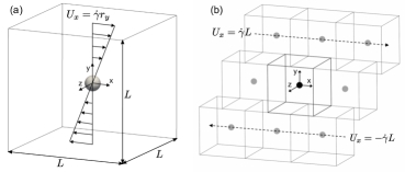
Figure 1: Schematic diagrams of the simulation setup: (a) single-particle system and (b) the sliding cell interpretation of Lees–Edwards boundary conditions. Here $U_{x}=\dot{\gamma}r_{y}$ represents the velocity of the mean shear flow; and $L$ is the box length of the cubic domain. In (b), the image cells along the vorticity direction are not shown for simplicity.

II.3 Boundary conditions

To explain the boundary conditions of the sheared system, the single-particle system that is applied in Sec. III.1 is taken as an example. Fig. 1 shows schematic diagrams of the simulation system. One particle is located in the center $(r_{x}=r_{y}=r_{z}=0)$ of a cubic domain of $[-L/2,\,L/2]^{3}$, where $L$ is the box length of the domain. Here $x,y$, and $z$ indicate the flow, velocity-gradient, and vorticity directions, respectively. Then, simple shear flow $\bm{U}=\dot{\gamma}r_{y}\bm{e}_{x}$ is imposed by the time-dependent oblique coordinate system explained in Appendix A, where $\bm{e}_{i}~{}(i=x,y,z)$ is the Cartesian basis set. The corresponding velocity boundary conditions at the faces of the system are naturally established by the periodicity as follows:

$$\bm{u}(L/2,r_{y},r_{z}) =\bm{u}(-L/2,r_{y},r_{z}),$$ (20)

$$\bm{u}(r_{x},L/2,r_{z}) =\bm{u}(r_{x}-\gamma L,-L/2,r_{z})-\dot{\gamma}L\bm{e}_{x},$$ (21)

$$\bm{u}(r_{x},r_{y},L/2) =\bm{u}(r_{x},r_{y},-L/2),$$ (22)

where the simple periodic boundary conditions for the flow (Eq. (20)) and vorticity (Eq. (22)) directions and the shear periodic boundary condition for the velocity-gradient (Eq. (21)) direction are established. The periodic boundary conditions for the conformation tensor are the same as Eqs.(20)-(22) except that the last term in Eq.(21) is not included. Lees–Edwards boundary conditions for particles can be interpreted as a sliding cell expression, as shown in Fig. 1(b). Initially, the image cells are aligned along all directions infinitely. Under simple shear flow, the upper and lower image cell layers stacked in the velocity-gradient direction slide in the flow direction with velocity $U_{x}=\pm\dot{\gamma}L$. The position and velocity of the particle going across the top and bottom faces of the main cell are modified as if the particle moved into the sliding image cell. These periodic boundary conditions in our method are preferred in evaluating bulk suspension rheology without the influence of the shear-driving walls. In our previous study, using this boundary condition, 3D steady shear simulations for a single-particle viscoelastic suspension system were conducted (Matsuoka et al., 2020). Similar periodic boundary conditions were adopted for two-dimensional (2D) steady shear flow simulations (Hwang et al., 2004; Jaensson et al., 2015) and 3D dynamic shear flow simulations (D’Avino et al., 2013) of viscoelastic suspensions. In contrast to recent 3D steady shear flow simulations for many-particle systems which utilize walls to impose the shear flow (Yang & Shaqfeh, 2018b; Vázquez-Quesada et al., 2019), this study presents for the first time wall-free 3D steady shear flow simulations for a many-particle viscoelastic suspension system. The details of the numerical solution procedure are described in Appendix B.

III Results and discussion

In this section, the developed DNS method is applied to the rheological evaluations of sheared viscoelastic suspensions. First, to show the validity of rheological evaluations by our developed DNS method, the suspension viscosity of the single-particle dilute system is evaluated and compared to previously reported numerical and theoretical results. Further examinations of our DNS method are explained in Appendix C. Next, detailed rheological evaluation is conducted for a semi-dilute viscoelastic suspension, which contains many particles immersed in a multi-mode Oldroyd-B fluid, and the results are compared with previously reported experimental results.

III.1 Suspension rheology of single-particle system

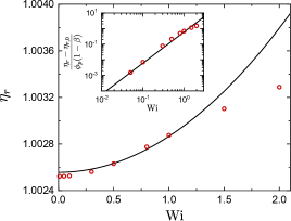
Figure 2: The $\rm{Wi}$ dependence of the relative viscosity of a dilute Oldroyd-B suspension at $\beta=0.5$. The inset shows the $\rm{Wi}$ dependence of the thickening part of $\eta_{r}$. Red open circles represent results from this work. The black lines correspond to the theoretical prediction by Einarsson et al. (2018) using Eq. (23).

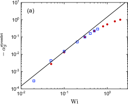
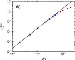
Figure 3: The $\rm{Wi}$ dependence of (a) stresslet $\alpha_{S}^{\rm{stresslet}}$ and (b) particle-induced fluid stress $\alpha_{S}^{\rm{fluid}}$ contributions to the suspension viscosity at $\beta=0.5$. Red filled circles represent results from this work, and blue squares are the DNS results by Einarsson et al. (2018). The black line is plotted according to the theory by Einarsson et al. (2018).

A perturbation analysis of the suspension in a single-mode Oldroyd-B medium by Einarsson et al. (2018) predicted the shear-thinning in the stresslet and the shear-thickening in the particle-induced fluid stress at $O(\phi_{p}\rm{Wi}^{2})$:

$$\eta_{r}=1+2.5\phi_{p}+\phi_{p}(1-\beta)(\alpha_{S}^{\rm{stresslet}}+\alpha_{S}^{\rm{fluid}}),$$ (23)

where $\alpha_{S}^{\rm{stresslet}}=-1.43\rm{Wi}^{2}-0.06(1-\beta)\rm{Wi}^{2}$ and $\alpha_{S}^{\rm{fluid}}=2.05\rm{Wi}^{2}+0.03(1-\beta)\rm{Wi}^{2}$ are the contributions from the stresslet and particle-induced fluid stress (Sec. II.2), respectively. DNS of a single particle in an Oldroyd-B medium by Yang and Shaqfeh (Yang & Shaqfeh, 2018a) showed shear-thickening in the particle-induced fluid stress around a particle. To confirm that the method developed in this work can be applied for rheological evaluation, the viscosity and the bulk stress of a single-particle suspension in an Oldroyd-B medium is evaluated. The numerical setup is the same as that explained in Sec.II.3 (Fig. 1(a)). The system size is $L=128\Delta$ and the particle radius and interfacial thickness are $a=8\Delta$ and $\xi=2\Delta$, respectively. This corresponds to $\phi_{p}=0.001023$. All calculations are conducted with a small Reynolds number $\rm{Re}\leq 0.051$, i.e., the effect of inertia is negligible.

Fig. 2 shows the $\rm{Wi}$ dependence of the steady-state relative shear viscosity, $\eta_{r}=\langle\sigma_{xy}^{\rm{sus}}\rangle/(\eta_{0}\dot{\gamma})$, of the single-mode Oldroyd-B suspension at $\beta=0.5$. Shear-thickening is observed in the suspension viscosity for increasing $\rm{Wi}$. In the $\rm{Wi}\rightarrow 0$ limit, the relative viscosity ($\eta_{r,0}=1.002522$, which is obtained from fitting the numerical results at low $\rm{Wi}$ by using $\eta_{r}=\eta_{r,0}+b_{\rm{f}}\rm{Wi}^{2}$) approaches Einstein’s theoretical value, $\eta_{r}=1+2.5\phi_{p}=1.002557$. The small discrepancy from the theoretical value in $\eta_{r,0}$ is mostly attributed to the stresslet contribution and is suggested to be due to the diffused interface of the particle surface in SPM. The developed method reveals the $\rm{Wi}^{2}$ dependence as predicted by Eq. (23) at roughly $\rm{Wi}<1$; the inset of Fig. 2 shows this clearer, where the thickening part $\eta_{r}-\eta_{r,0}$ in the relative viscosity is shown. However, at $\rm{Wi}\gtrsim 1$, shear-thickening is slower than $\rm{Wi}^{2}$ growth because the perturbation analysis is expected to be valid at $\rm{Wi}\ll 1$. For a more detailed comparison, $\alpha_{S}^{\rm{stresslet}}$ and $\alpha_{S}^{\rm{fluid}}$ at $\beta=0.5$ are evaluated separately as

$$\alpha_{S}^{\rm{stresslet}} =\frac{N\langle S_{xy}\rangle/V-\eta_{0}\dot{\gamma}(\eta_{r,0}-1)}{\eta_{0}\dot{\gamma}\phi_{p}(1-\beta)},$$ (24)

$$\alpha_{S}^{\rm{fluid}} =\frac{N\langle\Sigma_{xy}\rangle/V-\eta_{p}\dot{\gamma}}{\eta_{0}\dot{\gamma}\phi_{p}(1-\beta)},$$ (25)

as shown in Fig. 3 with a previous DNS result obtained by using a surface-conforming mesh (Einarsson et al., 2018); the results agree with the DNS by Einarsson et al.. By comparing with DNS results, the $O(\rm{Wi}^{2})$ prediction (solid line) is found to be valid at $\rm{Wi}\lesssim 0.3$ for $\alpha_{S}^{\rm{stresslet}}$ and $\rm{Wi}\lesssim 0.5$ for $\alpha_{S}^{\rm{fluid}}$. At higher $\rm{Wi}$ values, the $\rm{Wi}$ dependence is slower than $\rm{Wi}^{2}$ growth, which is observed both in $\left|\alpha_{S}^{\rm{stresslet}}\right|$ and in $\alpha_{S}^{\rm{fluid}}$.

The agreement between the obtained results and those from perturbation theory and a previous DNS study verifies the capability of the developed SPM for the rheological evaluation of suspensions in viscoelastic media. By using the presented numerical method, the influence of $\beta$ on the rheology of a dilute suspension in an Oldroyd-B medium has been explored in detail (Matsuoka et al., 2020).

III.2 Suspension rheology of many-particle system

For dilute and semi-dilute particle concentrations, the rheology of many-particle systems is studied in contrast to the single-particle system considered in Sec. III.1. The numerical condition in this study is decided in accordance with the experimental conditions previously reported by Yang & Shaqfeh (2018b). They have performed detailed rheological measurements of a viscoelastic medium, including the elongation viscosity, in addition to the rheological measurements of a suspension system. Thus, their experimental results are likely to be the most complete dataset available for the quantitative rheological evaluation by DNS. Furthermore, as mentioned in their paper, wall effects for the rheological measurements are expected to be negligible in their experiments, which is suitable for our shear periodic boundary condition explained in Sec. II.3.

Mode $k$		$\eta_{p}^{(k)}~{}\rm{(Pa\cdot s)}$		$\lambda^{(k)}~{}\rm{(s)}$		$\eta_{p}^{(k)}\lambda^{(k)}~{}\rm{(Pa\cdot s^{2})}$
1		0.67		3.2		2.144
2		0.66		0.26		0.172
3		0.25		0.032		$8.0\times 10^{{-3}}$
4		0.44		0.002		$8.8\times 10^{-4}$
Solvent		1.46		–		–

Table 1: Parameters for a four-mode Oldroyd-B fluid. The values are from Table I of Yang & Shaqfeh (2018b), which are estimated from the small-amplitude oscillatory shear measurement of a Boger fluid.

III.2.1 Numerical conditions

The system and particle sizes are the same as in Sec. III.1, i.e., $L=128\Delta$, $a=8\Delta,and\xi=2\Delta$. Considering dilute to semi-dilute particle concentrations, one has $\phi_{p}=0.001,0.025,0.05$, and $0.1$ by setting the number of particles to 1, 24, 49, and 98, respectively. The initial positions of the particles are set to be randomly distributed and non-overlapping, with the inter-surface distance set to at least $2\Delta$. For each $\phi_{p}$ except for $\phi_{p}=0.001$ (single-particle system), at least three different realizations are calculated. An experimental result reported by Yang & Shaqfeh (2018b) is considered where the rheology of a suspension in a Boger fluid consisting of polybutene, polyisobutylene, and kerosene was evaluated. For the rheological characterization of the Boger fluid, both steady-shear and small-amplitude oscillatory shear (SAOS) measurements were reported (Yang & Shaqfeh, 2018b). In principle, the parameters in the Oldroyd-B model can be estimated from either the steady-shear or SAOS data; however, due to the limited range of the rate window, the zero-shear first NSD was available only from the SAOS data. Furthermore, in their experiment, the suspension viscosity begins to show shear-thickening at $\dot{\gamma}\approx 0.2{\rm s}^{-1}$, a shear rate that is below the rate window of steady-shear $N_{1}$ data. Therefore, the parameters estimated from the SAOS data listed in Table 1 are used here to solve the corresponding four-mode Oldroyd-B fluid as a suspending medium. Note that Yang and Shaqfeh also reported the DNS prediction with experimental data (Yang & Shaqfeh, 2018b), where, in contrast to this work, the single-mode Oldroyd-B model with parameters estimated from the steady-shear property of the suspending Boger fluids resulted in an underestimation of the suspending viscosity. The discrepancy between their simulation and experimental results is discussed later (Sec. III.2.3).

After the steady state is reached, the viscometric functions of the many-particle suspension are time-averaged over at least $\dot{\gamma}\Delta t=10$ from $\dot{\gamma}t\geq 10\max\{1,\dot{\gamma}\lambda^{(1)}\}$. Finally, the time-averaged values are ensemble-averaged over different realizations to obtain the viscometric functions of bulk suspensions. The error bars in the following figures correspond to three times the standard deviation from the sample mean. The Weissenberg number is defined based on the longest relaxation time $\lambda^{(1)}=3.2~{}$s as ${\rm Wi}=\dot{\gamma}\lambda^{(1)}$. All calculations were conducted at a small Reynolds number $\rm{Re}\leq 0.018$ where effect of inertia is not significant.

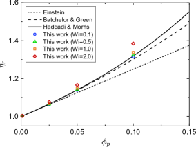
Figure 4: The $\phi_{p}$ dependence of the relative viscosity of suspensions at $\rm{Wi}=0.1$ (blue circles), $0.5$ (green triangles), $1.0$ (orange squares), and $2.0$ (red diamonds). The short-dashed and long-dashed lines correspond to the theoretical predictions for a Newtonian suspension by Einstein Einstein (1911) and Batchelor-Green Batchelor & Green (1972), respectively. The empirical prediction from Haddadi and Morris Haddadi & Morris (2014) is shown as a solid line.

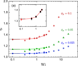
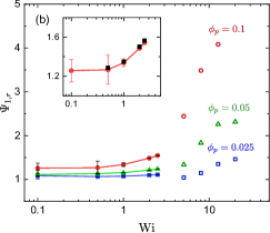
Figure 5: Viscometric functions of suspensions as functions of $\rm{Wi}$ and $\phi_{p}$: (a) relative viscosity and (b) relative first NSD coefficient of suspensions. The closed symbols are simulated results from this work, and the open symbols are experimental results from Yang & Shaqfeh (2018b). The blue squares, green triangles, and red circles correspond to the results for $\phi_{p}=0.025,\,0.05,$ and $0.1$, respectively. Experimental $\eta_{r}$ and $\Psi_{1,r}$ are calculated using $\eta(\phi_{p},\dot{\gamma})$ and $\Psi_{1}(\phi_{p},\dot{\gamma})$ reported by Yang & Shaqfeh (2018b). The dashed lines in (a) are values predicted by the Eilers fit (Haddadi & Morris, 2014). Solid lines are guides to the eye. The insets in (a) and (b) show the DNS results at $\phi_{p}=0.1$ by the multi-mode model (red circles) and the effective single-mode model (black squares) explained in Sec. III.2.3.

III.2.2 Suspension viscosity and first NSD coefficient

Figure 4 shows the steady-state suspension viscosity normalized by $\eta_{0}$ for different $\rm{Wi}$ as functions of $\phi_{p}$; the theoretical trends for a Newtonian suspension in the creeping flow regime are also shown. Here, $\eta_{r}=1+2.5\phi_{p}+\alpha\phi_{p}^{2}$ where $\alpha=0$ for Einstein theory Einstein (1911) (short-dashed line) and $\alpha=5.2$ for Batchelor–Green theory Batchelor & Green (1972) (long-dashed line). In addition, the empirical Eilers fit for the numerical result of Newtonian suspensions by Haddadi & Morris (2014), $\eta_{r}=\left(1+\frac{1}{2}[\eta]\phi_{p}/(1-\phi_{p}/\phi_{p,m})\right)^{2}$, with $[\eta]=2.5$ and $\phi_{p,m}=0.63$, is also plotted (solid line). At $\rm{Wi}=0.1$, the suspension viscosity agrees well with the predictions by Batchelor–Green and Eilers fit for Newtonian suspensions. This is expected because the polymer stress is expected to fully relax at $\rm{Wi}\ll 1$ to exhibit almost Newtonian behavior. In contrast, as $\rm{Wi}$ increases, the suspension viscosity increases to be above the prediction for Newtonian suspensions.

In Fig. 5, the viscosity (Fig. 5(a)) and first NSD coefficient (Fig. 5(b)) as functions of $\rm{Wi}$ are compared with the experimental result by Yang & Shaqfeh (2018b) for different $\phi_{p}$. The viscosity at the $\rm{Wi}\to 0$ limit calculated by Eilers fit in Fig. 4 for each $\phi_{p}$ is also shown in Fig. 5(a). The numerical results of this work agree quantitatively with the experimental results up to a semi-dilute case of $\phi_{p}=0.1$. The first NSD coefficient of the suspension, $\Psi_{1}=\langle\sigma_{xx}^{\rm{sus}}-\sigma_{yy}^{\rm{sus}}\rangle/\dot{\gamma}^{2}$, normalized by that of the medium is shown in Fig. 5(b). As $\rm{Wi}$ increases, $\Psi_{1,r}$ also increases. Although the ranges of $\rm{Wi}$ of the experimental and numerical results do not overlap, the numerical results of this work smoothly connect with the experimental results.

Note that, while the DNS results agree with the experimental $\eta_{r}$, the DNS using an Oldroyd-B model reported by Yang & Shaqfeh (2018b) underestimated it. The main difference between this work and that of Yang–Shaqfeh is the estimation of the zero-shear $N_{1}$ of the suspending Boger fluid; $N_{1}$ from the SAOS measurement is approximately twice as large as that from the steady-shear measurement; the difference occurs because the steady-shear measurement did not reach the terminal region and showed a decreased $N_{1}$. These results suggest that predicting suspension shear-thickening at around $\rm{Wi}=1.0$ requires an accurate estimation of $N_{1}$ of the suspending medium in the shear-rate range where the shear-thickening starts to occur. For the Boger fluid used in  Yang & Shaqfeh (2018b), this range is supposed to be the terminal region, which cannot be reached by the steady-shear measurement. The estimation of $N_{1}$ directly affects the level of polymer stress around the particles, because, as past studies on dilute systems have revealed (Yang & Shaqfeh, 2018a; Matsuoka et al., 2020), the elastic stress due to the stretched conformation nearby upstream of the particles contributes to the macroscopic shear stress. In Yang & Shaqfeh (2018b), their model’s underestimation of the medium’s elongational property is argued to be one reason why their DNS prediction underestimates the measured shear-thickening of suspensions. Although our four-mode Oldroyd-B model shows slightly higher elongational viscosity than that by the single-mode model used in Yang & Shaqfeh (2018b), our multi-mode model still underestimates the measured elongational viscosity of the medium. This result suggests that suspension shear-thickening in Boger fluids at around $\rm{Wi}=1.0$ can be predicted with the Oldroyd-B model without additional modelling of the elongational response.

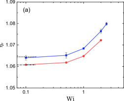
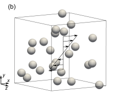
Figure 6: DNS results at $\phi_{p}=0.025$: (a) suspension viscosity for single-particle (red circles) and many-particle (blue squares) systems; and (b) microstructure in a many-particle system at ${\rm Wi}=2.0$. In (a), the black lines are predictions for Newtonian suspensions according to the theories of Batchelor–Green (dashed, $\phi_{p}=0.02454$ for many-particle systems) and Einstein (dot-dashed, $\phi_{p}=0.02430$). Solid lines are guides to the eye.

To demonstrate the difference between many-particle and single-particle systems at dilute conditions, a single-particle simulation is conducted at $\phi_{p}\approx 0.025$ by setting the particle radius $a=23\Delta$ and system size $L=128\Delta$ in the single-particle system shown in Fig. 1(a); the Reynolds number is kept small ($\rm{Re}=0.076$). Because of the periodic boundary conditions, this single-particle system corresponds to the sheared cubic array system shown in Fig. 1(b). In Fig. 6(a), the suspension viscosity between single-particle (cubic array structure) and many-particle (random structure) systems is compared. The single-particle result indicates lower viscosity, whereas the shear-thickening behavior is almost the same as that of the many-particle system. At $\rm{Wi}\rightarrow 0$, the viscosity from the single-particle system agrees with the Einstein prediction. This also agrees with the results of a cubic array system in a Newtonian medium (Nunan & Keller, 1984; Phan-Thien et al., 1991). Correspondingly, $\langle S_{xy}\rangle$ for the single-particle system agrees with the Einstein stresslet (the inset of Fig. 9(a)). Fig. 6(b) shows the microstructure of the many-particle system in a sheared steady state at $\phi_{p}=0.025$ and ${\rm Wi}=2$. In many-particle systems, particles are randomly dispersed and occasionally get very close to each other, which induces the large stresslet contribution. On the other hand, in the single-particle system, the inter-particle distance remains above a certain level as shown in Fig. 1(b). Therefore, the viscosity shift between the two systems is attributed to the difference in the stresslet contribution by microstructures. Note that particle alignment, which is sometimes observed experimentally in suspensions with viscoelastic fluids (Michele et al., 1977; Scirocco et al., 2004), is not be observed at all $\phi_{p}$ and ${\rm Wi}$ in our study. This suggests that our simulation conditions are out of range for an alignment critical condition predicted by DNS using Oldroyd-B and Giesekus matrices  (Hwang & Hulsen, 2011; Jaensson et al., 2016). The result from this work, showing that the suspension microstructure affects the viscosity even at dilute conditions, is consistent with the results of a previous study (Vázquez-Quesada et al., 2019). Furthermore, similar shear-thickening behavior independent of the microstructures suggests that the shear-thickening at dilute conditions is mainly originated from the polymer stress in the vicinity of a particle, which is consistent with a previous study (Yang & Shaqfeh, 2018a, b).

III.2.3 Relaxation mode decomposition of polymer stress

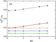
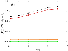
Figure 7: Proportions of each relaxation mode in the polymer stress contribution (for $k$=1 (red circles), 2 (orange triangles), 3 (green squares), and 4 (blue diamonds), and the sum of the mode contributions (black lower triangle)): (a) shear viscosity and (b) first NSD coefficient at $\phi_{p}=0.1$. The values of $\langle\eta_{p}^{(k)}\rangle$ and $\langle\Psi_{1,p}^{(k)}\rangle$ are normalized by $\eta_{0}$ and $\Psi_{1}(\phi_{p}=0)=2\sum_{k=1}^{4}\eta_{p}^{(k)}\lambda^{(k)}$, respectively. Note that the stresslet contributions are not included in the figure. Lines are guides to the eye. By definition, the order of $\langle\eta_{p}^{(k)}\rangle$ and $\langle\Psi_{1,p}^{(k)}\rangle$ at $\rm{Wi}\rightarrow 0$ corresponds to the order of $\eta_{p}^{(k)}$ and $\eta_{p}^{(k)}\lambda^{(k)}$ in Table. 1, respectively. That is why $\langle\eta_{p}^{(4)}\rangle>\langle\eta_{p}^{(3)}\rangle$ in (a). In (b), $\langle\Psi_{1,p}^{(4)}\rangle$ is not shown because it is smaller than $\langle\Psi_{1,p}^{(3)}\rangle$.

In the modelling of the suspensions in a Boger fluid, the four-mode Oldroyd-B model is used for the suspending medium. The separate contributions from each relaxation mode to the suspension shear-thickening is discussed. The viscosity and the first NSD coefficient from the $k$-th mode are defined as $\langle\eta_{p}^{(k)}\rangle\equiv[\int_{D_{V}}(1-\lfloor\phi\rfloor)\sigma_{p,xy}^{(k)}d\bm{r}/V]/\dot{\gamma}$ and $\langle\Psi_{1,p}^{(k)}\rangle\equiv[\int_{D_{V}}(1-\lfloor\phi\rfloor)(\sigma_{p,xx}^{(k)}-\sigma_{p,yy}^{(k)})d\bm{r}/V]/\dot{\gamma}^{2}$ ($k=1,2,3,4$), respectively. Figure 7 shows the $k$-th viscosity normalized by $\eta_{0}$and the $k$-th first NSD coefficient normalized by $\Psi_{1}$ at $\phi_{p}=0$ as functions of $\rm{Wi}$ at $\phi_{p}=0.1$. Both for the viscosity (Fig. 7(a)) and for the first NSD coefficient (Fig. 7(b)), only the first mode exhibits shear-thickening, whereas the other faster modes show a rate-independent contribution. This is expected, because the $\rm{Wi}$ considered here is much smaller than $\lambda^{(1)}/\lambda^{(2)}=12.3$; the elastic stress from the second and subsequent modes fully relaxes to show a zero-shear response.

The results in Fig. 7 suggest that single-mode modelling for the suspending medium is likely to be sufficient to predict the rheological response at the $\rm{Wi}\leq 2.5$ considered in the current simulation. If only the first mode is responsible for the polymer stress, the effective parameters for a single-mode Oldroyd-B fluid are determined from Table 1 to be $\lambda^{\rm eff}=\lambda^{(1)}=3.2$ s, $\eta_{p}^{\rm eff}=\eta_{p}^{(1)}=0.67$ Pa$\cdot$s, and $\eta_{s}^{\rm eff}=\eta_{s}+\sum_{k=2}^{4}\eta_{p}^{(k)}=2.81$ Pa$\cdot$s, resulting in $\beta^{\rm{eff}}=\eta_{s}^{\rm{eff}}/\eta_{0}=0.807$. This effective $\beta$ value is smaller than the $\beta=0.9$ used in DNS (Yang & Shaqfeh, 2018b), which underpredicted the experimental suspension rheology. In the inset of Fig. 5, the DNS result of the presented effective single-mode model (black squares) is compared with that of the multi-mode model (red circles), showing good agreement with the multi-mode results and thus experimental results (Yang & Shaqfeh, 2018b). This difference between the $\beta$ values originates from the difference in the estimation of the zero-shear NSD coefficient of the Boger fluid that was mentioned in Sec. III.2.2.

In the system considered in this work, only $\lambda^{(1)}$ is relevant to the studied range of $\rm{Wi}$. Whether single-mode modelling can be used for the quantitative prediction of suspension rheology for other types of suspending media depends on both the relaxation time distribution of the fluid and the distribution of the local shear-rate in the fluid, which is dependent on the fluid rheology as well as $\phi_{p}$. In Sec. III.2.5, we study how the local shear-rate distribution, flow pattern, and the elastic stress development change with $\phi_{p}$ and $\rm{Wi}$.

III.2.4 Decomposition of the total suspension stress

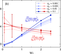
Figure 8: Contributions to the total suspension stress from stresslet $\bm{S}$ (red) and particle-induced fluid stress $\bm{\Sigma}$ (blue) at $\phi_{p}=0.001$ to 0.1 (from light to dark color): (a) Contributions to the total shear stress normalized by $\eta_{0}\dot{\gamma}a^{3}$; and (b) contributions to the total first NSD normalized by $\eta_{0}\lambda^{(1)}\dot{\gamma}^{2}a^{3}$. Solid lines are guides to the eye.

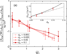
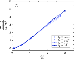
Figure 9: Viscoelastic contributions to the total suspension shear stress as a function of the effective Weissenberg number at $\phi_{p}=0.001$ to 0.1 (from light to dark color). (a) Stresslet contribution to shear stress. The ordinate represents the polymeric part of $\langle S_{xy}\rangle$; $\langle S_{xy}\rangle-\langle S_{xy,0}\rangle$ where $\langle S_{xy,0}\rangle$ is the Newtonian part of $\langle S_{xy}\rangle$ represented by Eq. (26). The inset shows the $\phi_{p}$ dependence of $\langle S_{xy}\rangle$ at $\rm{Wi}=0.1$ (red circles). The result from single-particle simulation at $\phi_{p}=0.025$ is also shown (red square). The black lines are predictions according to theories of Einstein (dotted), Batchelor–Green (dot-dashed), and Eilers fit by Haddadi & Morris (solid). The contributions for the shear stress are normalized by $\eta_{0}\dot{\gamma}a^{3}$. (b) Particle-induced fluid stress contributions for shear stress. The effective Weissenberg number $\widetilde{\rm{Wi}}$ is defined with the average strain-rate in the fluid region at each $\phi_{p}$. In both panels, the red and blue solid lines are guides to the eye.

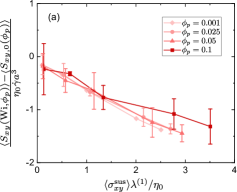
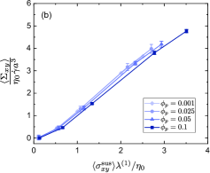
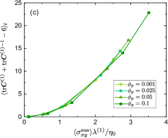
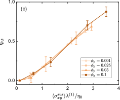
Figure 10: Viscoelastic contributions to the total suspension shear stress as a function of the suspension shear stress at $\phi_{p}=0.001$ to $0.1$ (from light to dark color): (a) stresslet, (b) particle-induced fluid stress, (c) normalized polymer dissipation function of the first relaxation mode, and (d) the thickening portion of the relative viscosity. The suspension shear stress in the abscissa in each panel is non-dimensionalized as $\langle\sigma_{xy}^{\rm{sus}}\rangle\lambda^{(1)}/\eta_{0}$. Solid lines are guides to the eye.

The $\phi_{p}$ dependence of the shear-thickening of the suspension in the Oldroyd-B medium is discussed. The contributions from the stresslet, $\bm{S}$, and the particle-induced fluid stress, $\bm{\Sigma}$, to the suspension rheology are shown in Fig. 8, where the shear component is normalized by $\eta_{0}\dot{\gamma}a^{3}$ to correspond to a non-dimensional viscosity, and the first NSD component is normalized by $\eta_{0}\lambda^{(1)}\dot{\gamma}^{2}a^{3}$ to correspond to the non-dimensional NSD coefficient. For the viscosity component in Fig. 8(a), as $\rm{Wi}$ increases, the stresslet viscosity, $\langle S_{xy}\rangle/(\eta_{0}\dot{\gamma}a^{3})$, decreases, and the particle-induced fluid viscosity, $\langle\Sigma_{xy}\rangle/(\eta_{0}\dot{\gamma}a^{3})$, increases more than the change in the stresslet viscosity. Specifically, at $\rm{Wi}=2.0$, the decrease in $\langle S_{xy}\rangle/(\eta_{0}\dot{\gamma}a^{3})$ is less than two, but the increase in $\langle\Sigma_{xy}\rangle/(\eta_{0}\dot{\gamma}a^{3})$ is more than three for all $\phi_{p}$ considered. This result clearly demonstrates that the shear-thickening of the suspension viscosity originates from an increase in $\langle\Sigma_{xy}\rangle$, which is consistent with what has been reported in previous work (Yang & Shaqfeh, 2018a, b; Matsuoka et al., 2020). As $\phi_{p}$ increases, the increase in $\langle\Sigma_{xy}\rangle/(\eta_{0}\dot{\gamma}a^{3})$ with $\rm{Wi}$ is enhanced, whereas the decrease in $\langle S_{xy}\rangle/(\eta_{0}\dot{\gamma}a^{3})$ with $\rm{Wi}$ remains slow, which explains the enhancement of the shear-thickening with $\phi_{p}$ shown in Fig. 5(a). For the first NSD component (Fig. 8(b)), the general trends with respect to $\rm{Wi}$ and $\phi_{p}$ are similar to that of the viscosity component. These trends were also reported in a previous numerical study up to $\rm{Wi}\leq 1.0$ (Yang & Shaqfeh, 2018b). Because $N_{1}$ is very small and $N_{1}\propto\langle S_{xx-yy}\rangle$ at the $\rm{Wi}\to 0$ limit, the numerical fluctuation in calculating such a small value is large for $\langle S_{xx-yy}\rangle/(\eta_{0}\lambda^{(1)}\dot{\gamma}^{2}a^{3})$ at $\rm{Wi}\leq 0.5$.

The reduction rate of the stresslet viscosity with $\rm{Wi}$ does not strongly depend on $\phi_{p}$. Therefore, $\langle S_{xy}\rangle/(\eta_{0}\dot{\gamma}a^{3})$ is mainly determined by that at the $\rm{Wi}\to 0$ limit. This reduction of $\langle\bm{S}\rangle/(\eta_{0}\dot{\gamma}a^{3})$ with $\rm{Wi}$ indicates the reduced viscous traction on the particles that originates from the increased fraction of the elastic energy dissipation with $\rm{Wi}$, which is also related to the slowdown of the particle rotation rate with $\rm{Wi}$ discussed in Sec. C.2. The change of $\langle S_{xy}\rangle$ to that at the $\rm{Wi}\to 0$ limit, $\langle S_{xy,0}(\phi_{p})\rangle$, is plotted in Fig. 9(a) versus an effective Weissenberg number explained later; in Fig. 10(a), it is plotted against the suspension shear stress $\langle\sigma_{xy}^{\rm{sus}}\rangle$ normalized by $\eta_{0}/\lambda^{(1)}$. The numerical result for $\langle S_{xy}\rangle$ at $\rm{Wi}=0.1$ depicted in the inset of Fig. 9(a) almost agrees with the theoretical Batchelor–Green stresslet, $\langle S_{xy,0}\rangle/\left(\eta_{0}\dot{\gamma}a^{3}\right)=\left(4\pi/3\right)(2.5+\alpha\phi_{p})$ for $\phi_{p}\leq 0.05$, and with the empirical Eilers stresslet fitted for numerical results by Haddadi & Morris (2014):

$$\frac{\langle S_{xy,0}\rangle}{\eta_{0}\dot{\gamma}a^{3}}=\frac{4\pi}{3\phi_{p}}\left[\left(1+\frac{\frac{1}{2}[\eta]\phi_{p}}{1-\phi_{p}/\phi_{p,m}}\right)^{2}-1\right],$$ (26)

for $\phi_{p}\leq 0.1$. Based on this observation, $\langle S_{xy,0}\rangle$ in Fig. 9(a) is calculated with Eq. (26). In the suspension, a local shear rate can be larger than the applied rate $\dot{\gamma}$. To take this into account, the effective Weissenberg number $\widetilde{{\rm Wi}}=\tilde{\dot{\gamma}}\lambda^{(1)}$ is defined by using the average shear rate $\tilde{\dot{\gamma}}(\phi_{p},{\rm Wi})=\sqrt{\langle 2\bm{D}:\bm{D}\rangle_{\rm{f}}}$, where $\langle A\rangle_{\rm{f}}=\int_{D_{V}}\left(1-\lceil\phi\rceil\right)Ad\bm{r}/\left[\left(1-\phi_{p}\right)V\right]$ represents the volume average of a local variable $A$ over the fluid region and $\lceil\cdot\rceil$ indicates the ceiling function. For dilute cases ($\phi_{p}\leq 0.05$), the changes of the stresslet viscosity as a function of $\widetilde{\rm{Wi}}$ in Fig. 9(a) nearly coincide. For a semi-dilute case ($\phi_{p}=0.1$), the the stresslet viscosity change agrees with the dilute cases for $\widetilde{\rm{Wi}}\lesssim 1.5$. At higher $\widetilde{\rm{Wi}}\gtrsim 1.5$, the negative slope of the stresslet viscosity becomes smaller than that in the dilute cases, though this change is not large compared to that at $S_{xy,0}(\phi_{p})/(\eta_{0}\dot{\gamma}a^{3})$. The change of $\langle S_{xy}\rangle/(\eta_{0}\dot{\gamma}a^{3})$ as a function of $\langle\sigma_{xy}^{\rm{sus}}\rangle\lambda^{(1)}/\eta_{0}$ in Fig. 10(a) shows a similar trend to that presented in Fig. 9(a). Although both ${\rm Wi}$ and $\phi_{p}$ increase $\widetilde{\rm{Wi}}$ and thus the elastic contribution in the fluid, the stresslet changes with $\phi_{p}$ and $\widetilde{\rm{Wi}}$ at $\phi_{p}=0.1$ are in opposite directions. This suggests the stresslet change due to microstructure at $\phi_{p}=0.1$ in addition to the change induced by polymer stress around individual particles. For $\langle S_{xx-yy}\rangle$, the large error at $\rm{Wi}=0.1$ makes it difficult to evaluate the analysis as it is done for $\langle S_{xy}\rangle$.

Next, the particle-induced fluid viscosity $\langle\Sigma_{xy}\rangle/(\eta_{0}\dot{\gamma}a^{3})$ that directly accounts for the elastic stress is discussed. At $\widetilde{\rm{Wi}}\lesssim 1$ in Fig. 9(b), the particle-induced fluid viscosity does not depend on $\phi_{p}$ because the elastic stress almost relaxes at $\widetilde{\rm{Wi}}\lesssim 1$. This region of $\widetilde{\rm{Wi}}$ corresponds to the zero-shear plateau of the suspension viscosity. At $\widetilde{\rm{Wi}}>1$, the increase of $\langle\Sigma_{xy}\rangle/(\eta_{0}\dot{\gamma}a^{3})$ with $\widetilde{\rm{Wi}}$ is enhanced as $\phi_{p}$ increases, indicating increased elastic stress with $\phi_{p}$. Since the elastic stress is dependent on flow-history and is not a simple function of the shear rate, the rate of increase of $\langle\Sigma_{xy}\rangle/(\eta_{0}\dot{\gamma}a^{3})$ with respect to $\widetilde{\rm{Wi}}$ changes with $\phi_{p}$. The plot of $\langle\Sigma_{xy}\rangle/(\eta_{0}\dot{\gamma}a^{3})$ as a function of $\langle\sigma_{xy}^{\rm{sus}}\rangle\lambda^{(1)}/\eta_{0}$ in Fig. 10(b) does not depend on $\phi_{p}$ for dilute conditions ($\phi_{p}\leq 0.05$), which is consistent with the previous work (Yang & Shaqfeh, 2018b). At a semi-dilute condition ($\phi_{p}=0.1$), $\langle\Sigma_{xy}\rangle/(\eta_{0}\dot{\gamma}a^{3})$ is slightly lower than that in the dilute cases, but the rate of increase is almost the same as that in the dilute condition. In Fig. 10(b), after a slow increase at $\langle\sigma_{xy}^{\rm{sus}}\rangle\lambda^{(1)}/\eta_{0}\ll 1$, the particle-induced fluid viscosity increases linearly to $\langle\sigma_{xy}^{\rm{sus}}\rangle\lambda^{(1)}/\eta_{0}\gtrsim 0.5$. The purely elastic contribution is directly evaluated by the polymer dissipation function, $\Phi_{p}^{(k)}=\left(\eta_{p}^{(k)}/(2(\lambda^{(k)})^{2})\right)\left\{{\rm tr}\bm{C}^{(k)}+{\rm tr}\bm{C}^{(k)-1}-6\right\}$. By using $\Phi_{p}$, an extra elastic contribution compared to a pure Oldroyd-B fluid is discussed in  Vázquez-Quesada et al. (2019). By definition, the polymer dissipation function is a scalar of $\bm{C}$ and thus independent of the direction of $\bm{C}$; ${\rm tr}\bm{C}-3$ and ${\rm tr}\bm{C}^{-1}-3$ measure the stretch and compression of $\bm{C}$, respectively. Fig. 10(c) shows the normalized polymer dissipation function of the first mode, $2\langle\Phi_{p}^{(1)}\rangle_{\rm f}(\lambda^{(1)})^{2}/\eta_{p}^{(1)}$, as a function of $\langle\sigma_{xy}^{\rm{sus}}\rangle\lambda^{(1)}/\eta_{0}$. Fig. 10(c) shows that the normalized polymer dissipation function at different $\phi_{p}$ collapses onto a single mastercurve, directly suggesting the similarity of the elastic contribution up to $\phi_{p}\leq 0.1$. Fig. 10(d) shows the shear-thickening part per particle defined as $\eta_{r,t}=[\eta_{r}(\phi_{p},\rm{Wi})-\eta_{r}(\phi_{p},\rm{Wi}\rightarrow 0)]/\phi_{p}$ as a function of suspension shear stress, where $\eta_{r}(\phi_{p},{\rm Wi}\rightarrow 0)$ is approximated by $\eta_{r}(\phi_{p},{\rm Wi}=0.1)$ because $\eta_{r}$ almost reaches the zero-shear plateau even at ${\rm Wi}=0.1$. Up to semi-dilute cases ($\phi_{p}\leq 0.1$), the increases in $\eta_{r,t}$ with $\langle\sigma_{xy}^{\rm{sus}}\rangle$ nearly coincides. Previous work (Yang & Shaqfeh, 2018b) reported that the variation of $\eta_{r,t}$ with $\langle\sigma_{xy}^{\rm{sus}}\rangle$ did not depend on $\phi_{p}$ for $\phi_{p}\leq 0.1$, which is also confirmed in this work.

III.2.5 Flow characterization of viscoelastic suspension

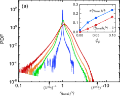
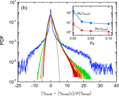
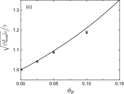
Figure 11: The $\phi_{p}$ and $\rm{Wi}$ dependence of the local strain-rate in the fluid region: (a) PDF of $\dot{\gamma}_{\rm{local}}$, where $\phi_{p}=0.1$ (red), 0.05 (orange), 0.025 (green), and 0.001 (blue), and the dotted and solid lines represent PDFs at $\rm{Wi}=0.1$ and $2.0$, respectively. The strain-rate is normalized by the imposed shear rate $\dot{\gamma}$, and the arrows indicate the first and second relaxation rates at $\rm{Wi}=2.0$. The inset shows the $\phi_{p}$ dependence of the mean and the standard deviation for Wi$=0.1$ (open symbols) and 2.0 (closed symbols). (b) PDF of $\dot{\gamma}_{\rm local}$ centered at the mean and normalized by standard deviation. The inset shows the $\phi_{p}$ dependence of the skewness and kurtosis. The line types are the same as those in (a). The dashed line indicates the standard Gaussian distribution. (c) Average local strain-rate, where blue squares and red circles correspond to Wi$=$0.1 and 2.0, respectively, and the line is the result from homogenization theory.

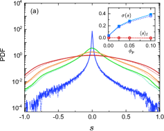
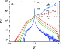
Figure 12: PDF of (a) strain-rate state $s$ and (b) irrotationality $E$ in the fluid region at various values of $\phi_{p}$ (0.1 (red), 0.05 (orange), 0.025 (green), and 0.001 (blue)). For each $\phi_{p}$, Wi=0.1 (dotted lines) and 2.0 (solid lines). The inset shows the $\phi_{p}$ dependence of the mean (red circles) and standard deviation (blue squares). The open and solid symbols in the inset indicate the results of ${\rm Wi}=0.1$ and $2.0$, respectively.

The probability density functions (PDF) of the local shear-rate $\dot{\gamma}_{\rm{local}}=\sqrt{2\bm{D}:\bm{D}}$ in the fluid domain for different $\phi_{p}$ and $\rm{Wi}$ are presented in Fig. 11(a). To sample the different particle configurations under flow for many-particle systems, the PDF is calculated from data over 25 snapshots per sample (in all, 75 snapshots) at the steady state by every $\dot{\gamma}\Delta t=0.215$ strain increment in three different initial particle configuration samples. Here $\dot{\gamma}_{\text{local}}\neq\dot{\gamma}$ is from the inhomogeneous flow near the particles, whereas $\dot{\gamma}_{\text{local}}=\dot{\gamma}$ is mainly from the region far from the particles where the flow is close to homogeneous shear flow. For the same $\rm{Wi}$, as $\phi_{p}$ increases, the shape of the PDF broadens and the peak position in the PDF gradually shifts towards large shear rate. This trend is clearly observed by the $\phi_{p}$ dependence of the mean $\langle\dot{\gamma}_{\rm local}\rangle_{\rm f}$ and standard deviation $\sigma(\dot{\gamma}_{\rm local})$ (the inset in Fig. 11(a)). Specifically, $\dot{\gamma}_{\text{local}}/\dot{\gamma}\lesssim 2$ for $\phi_{p}=0.001$ (single-particle result), while $\dot{\gamma}_{\text{local}}/\dot{\gamma}\lesssim 5$ for $\phi_{p}=0.1$. In general, a large shear-rate is effective in exciting the fast relaxation mode. At $\rm{Wi}=0.1$, the normalized first relaxation rate $\left(\lambda^{(1)}\dot{\gamma}\right)^{-1}=10$ is beyond the range of the local shear-rate for $\phi_{p}\leq 0.1$; therefore, the elastic response is irrelevant. At $\rm{Wi}=2$, where the first mode is relevant, the normalized second relaxation rate is $\left(\lambda^{(2)}\dot{\gamma}\right)^{-1}=6.15$, thus indicating that the second mode is still irrelevant to the elastic response. The PDF of the local shear rate which is centered at the mean and is normalized by the standard deviation, is shown in Fig. 11(b). At $\phi_{p}=0.001$, the normalized PDF is highly skewed and has fat tails. This corresponds to large positive values of the skewness $M_{3}(\dot{\gamma}_{\rm local})$ and kurtosis $M_{4}(\dot{\gamma}_{\rm local})$ (the inset in Fig. 11(b)), where $M_{n}(f)=\langle(f-\langle f\rangle_{\rm f})^{n}\rangle_{\rm f}/\sigma^{n}(f)$ is the normalized $n$-th-order statistics of $f$. As $\phi_{p}$ increases, the shape of PDF becomes closer to the Gaussian distribution (the dashed line), which corresponds to the decrease of $M_{3}(\dot{\gamma}_{\rm local})$ and $M_{4}(\dot{\gamma}_{\rm local})$. However, even at $\phi_{p}=0.1$, the PDF remain positively skewed, suggesting the asymmetric nature of the local shear rate distribution. In addition, the shape of PDF in Fig. 11 (a),(b) is not sensitive to the change in $\rm Wi$. Fig. 11(c) shows the root-mean-square of the local shear-rate $\tilde{\dot{\gamma}}=\sqrt{\langle\dot{\gamma}_{\text{local}}^{2}\ rangle_{\rm f}}$ as a function of $\phi$ at $\rm{Wi}=0.1$ and $2.0$. This average shear-rate increases with $\phi_{p}$ because the deformable fluid volume decreases with $\phi_{p}$. This phenomenon is expected to be common in solid suspensions. For comparison, a prediction for the average shear-rate by a homogenization theory for viscous fluid (Chateau et al., 2008),

$$\tilde{\dot{\gamma}}=\dot{\gamma}\sqrt{\frac{\eta_{r}(\phi_{p},\rm{Wi}\rightarrow 0)}{1-\phi_{p}}},$$ (27)

is drawn in Fig. 11(b), where $\eta_{r}$ in Eq. (27) is calculated with the Eilers fit by Haddadi & Morris (2014). Although the increasing trend of the average shear rate with $\phi_{p}$ is similar, the average shear-rate in the studied viscoelastic medium is slightly smaller than that predicted by Eq. (27). This is partly because Eq.(27) does not consider suspension microstructures explicitly. In fact, even for a Newtonian medium, Eq.(27) was reported to overestimate the suspension viscosity obtained by DNS at high $\phi_{p}$ (Alghalibi et al., 2018). From Fig. 11, the level of shear rate is hardly affected by ${\rm Wi}$ for ${\rm Wi}\leq 2$, and the fluctuation of $\dot{\gamma}_{\rm{local}}$ is mainly dominated by the solid volume fraction.

Next, the local flow pattern is discussed for different $\phi_{p}$ and $\rm{Wi}$. The topological aspect of the local flow pattern defined by $\nabla\bm{u}$ can be characterized by two scalars: multi-axiality of the strain-rate and irrotationality of $\nabla\bm{u}$ (Nakayama et al., 2016). The multi-axiality of flow in the incompressible flow is conveniently identified by the strain-rate state, which is defined as

$$s=\frac{3\sqrt{6}\det\bm{D}}{(\bm{D}:\bm{D})^{(3/2)}},$$ (28)

where $s\in[-1,1]$ by definition. For uniaxial elongational flow, where stretching in one direction and compression in the other two directions occur, $s>0$, whereas for biaxial elongational flow, where compression in one direction and stretching in the other two directions occur, $s<0$. For planar flow, where stretching occurs in one direction, compression occurs in another direction and no strain is found in the other direction, $s=0$. The magnitude of $s$ is determined by the relative magnitude of the three principal strain-rates of $\bm{D}$. Fig. 12(a) shows PDFs of $s$ for different $\phi_{p}$ and $\rm{Wi}$. Since homogeneous shear flow is planar flow, $s=0$ when $\phi_{p}\to 0$. As $\phi_{p}$ and/or $\rm{Wi}$ increase, the fraction of the planar flow indicated by $s=0$ decreases, and the fraction of triaxial flow indicated by $s\neq 0$ increases. This trend is also captured by the mean and standard deviation of $s$ (the inset in Fig. 12(a)).

The relative contribution of vorticity to the strain-rate is characterized by irrotationality, which is defined as

$$E=\frac{\sqrt{\bm{D}:\bm{D}}}{\sqrt{\bm{D}:\bm{D}}+\sqrt{\bm{\Omega}:\bm{\Omega}^{T}}},$$ (29)

where $\bm{\Omega}=(\nabla\bm{u}-\nabla\bm{u}^{T})/2$ is the vorticity tensor. By definition, $E\in[0,1]$. For rigid-body rotation, $E=0$; and $E=1$ for irrotational flow. As the vorticity contribution decreases, $E$ increases. Fig. 12(b) shows the PDF of the irrotationality for different $\phi_{p}$ and $\rm{Wi}$. In homogeneous simple shear flow at $\phi_{p}\to 0$, the flow is half rotational, i.e., $E=1/2$. As $\phi_{p}$ increases, the fraction of $E=1/2$ decreases, whereas the fraction of $E\neq 1/2$ increases. In particular, the fraction of $E>1/2$ is larger than that of $E<1/2$, indicating that the region with more irrotational flow than homogeneous shear flow increases with $\phi_{p}$. Since the vorticity contribution makes the fluid element avoid stretching, a large $E$ value suggests that the flow is strain-dominated to promote stretching of the conformation. As $\rm Wi$ increases, the width of the $E$ PDF gets narrower. The trend of the $E$ PDF with $\phi_{p}$ and ${\rm Wi}$ is summarized by the mean and standard deviation of $E$ (the inset in Fig. 12(b)). The insets in Figs. 12(a) and (b) indicate that the flow pattern as measured by $s$ and $E$ is mostly dominated by $\phi_{p}$. These changes in the PDFs of $s$ and $E$ reflect the modulation of the flow caused by the particle inclusion, which is further examined in the following section.

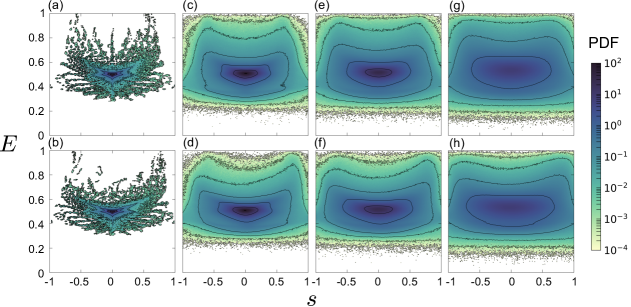
Figure 13: The 2D PDFs of strain-rate state $s$ and irrotationality $E$ in the fluid region: (a),(b) $\phi_{p}=0.001$; (c),(d) $\phi_{p}=0.025$; (e),(f) $\phi_{p}=0.05$; and (g),(h) $\phi_{p}=0.1$. The top and bottom row indicate the results at $\rm{Wi}=0.1$ and $2.0$, respectively. The contour lines correspond to ${\rm PDF}=10^{k}:k=-4,-3,-2,-1,0,1,2$.

To discuss the correlation between the strain-rate state and irrotationality and the spatial variation of the flow pattern, a joint PDF of $s$ and $E$ for different $\phi_{p}$ at $\rm{Wi}=0.1$ and $2.0$ is shown in Fig. 13; snapshots of $s$ and $E$ on a shear plane at different $\phi_{p}$ and $\rm{Wi}$ are presented in Figs. 14 and 15, respectively. The simple shear flow corresponds to $(s,E)=(0,1/2)$. At $\rm{Wi}=0.1$ and $\phi_{p}=0.001$ and 0.025 (Figs. 13(a) and (c), respectively), the $s-E$ distribution appears like the face of a fox; high-$E$ flow is actually non-planar high-$|s|$ flow, which forms the fox’s ears. At $\rm{Wi}=0.1$, the distribution of $s$ is almost symmetric for different $\phi_{p}$ (Fig. 13(a),(c),(e), and (g)), thus reflecting the fore-aft symmetry of the flow around a particle ($s$ and $E$ at $\phi_{p}=0.025$ in Fig. 14). For irrotational flow of $E>0.5$, the fraction of the planar flow of $s=0$ is relatively small, and hence, the triaxial flow of $s\neq 0$ is predominant. This reflects the flow in the upstream and downstream regions of the particles ($s$ and $E$ at $\phi_{p}=0.025$ in Fig. 14), where the flow is forced to avoid the particles to generate irrotational bifurcating (biaxial elongational) flow upstream and irrotational converging (uniaxial elongational) flow downstream (Einarsson et al., 2018; Yang & Shaqfeh, 2018a; Vázquez-Quesada et al., 2019; Matsuoka et al., 2020). As $\rm{Wi}$ increases, the distribution of $s$ at $E>1/2$ becomes asymmetric (Fig. 13(b),(d), and (f)); the fraction of $s>0$ is larger than that of $s<0$. This corresponds to symmetry breaking in the upstream and downstream flows around the particles with an increase of $\rm{Wi}$. As shown in the $E$ distribution at $\phi_{p}=0.025$ and $\rm{Wi}=2.0$ (Fig. 15), high-$E$ regions around a particle shift counter-clockwise with respect to the symmetric distribution at $\rm{Wi}=0.5$. Because of this change, in the upstream region of the particle, the vorticity contribution increases with $\rm{Wi}$, leading to a decrease in $E$, whereas $E$ in the downstream region does not change significantly. This change of flow patterns with $\rm{Wi}$ is attributed to the local flow modulation by large polymer stress gradients around particles, which was examined in detail in our previous study for a single-particle system (Matsuoka et al., 2020). Although ${\rm Wi}$ affects the local flow pattern around a particle, the microstructure does not change obviously with $\rm Wi$, as seen in Figs. 14 and 15.

In this study, our DNS of many-particle systems enables us to examine the effect of the particle volume fraction on the local flow patterns. As $\phi_{p}$ increases, the $s-E$ PDF spreads out widely (from left to right panels in Figs. 13). In addition to the increase in the fraction of the characteristic flow field around single particles, this $s-E$ distribution also reflects the spatial overlap of the characteristic flow field between particles, which is shown in Figs. 14 and 15. Especially, the high-$E$ fox ears in the $s-E$ PDF are smeared out with increased $\phi_{p}$ because the interaction between particles becomes predominant to modify the flow between particles. Fig. 16 shows the color contour of the strain-rate state at the highly irrotational region of $E\geq 0.65$ at $\rm{Wi}=2.0$. At the dilute condition of $\phi_{p}=0.025$, the highly irrotational region adjacent to each particle is isolated over most of the time (Fig. 16(b)). In contrast, as $\phi_{p}$ increases, additional bifurcating irrotational regions develop between particles when two particles get closer (Fig. 16(c)(d)).

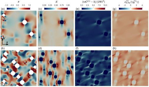
Figure 14: Spatial distribution of the flow pattern characterized by (a),(b) the strain-rate state $s$; (c),(d) irrotationality $E$; (e),(f) normalized polymer stretch of the first mode $(\text{tr}\bm{C}^{(1)}-3)/(2\rm{Wi}^{2})$; and (g),(h) the normalized shear stress of the first mode $\sigma_{p,xy}^{(1)}/(\eta_{p}^{(1)}\dot{\gamma})$ on a shear plane ($x,y$ plane) at $\rm{Wi}=0.5$. The top (a, c, e, g) and bottom (b, d, f, h) rows are the results at $\phi_{p}=0.025$ and $0.1$, respectively.

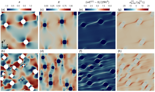
Figure 15: Spatial distribution of the flow pattern characterized by (a),(b) the strain-rate state $s$; (c),(d) irrotationality $E$; (e),(f) normalized polymer stretch of the first mode $(\text{tr}\bm{C}^{(1)}-3)/(2\rm{Wi}^{2})$; and (g),(h) the normalized shear stress of the first mode $\sigma_{p,xy}^{(1)}/(\eta_{p}^{(1)}\dot{\gamma})$ on a shear plane ($x,y$ plane) at $\rm{Wi}=2.0$. The top (a, c, e, g) and bottom (b, d, f, h) rows are the results at $\phi_{p}=0.025$ and $0.1$, respectively.

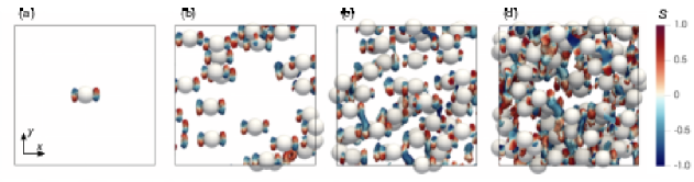
Figure 16: The isovolume visualization of a highly irrotational region at $\rm{Wi}=2.0$: (a) $\phi_{p}=0.001$, (b) $0.025$, (c) $0.05$, and (d) $0.1$. The isovolume represents a region where $E\geq 0.65$, and the color represents the strain-rate state $s$.

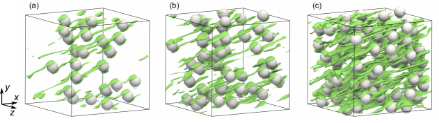
Figure 17: Polymer high-stretch region at $\rm{Wi}=2.0$: (a) $\phi_{p}=0.025$, (b) $0.05$, and (c) $0.1$. The isovolume of ${\rm tr}\bm{C}^{(1)}\geq 2(2\widetilde{\rm{Wi}}^{2}+3)$ is visualized in green, where the threshold is twice the value of $\text{tr}\bm{C}$ in the Oldroyd-B fluid under homogeneous shear flow.

Finally, the development of polymer stretch and polymer shear stress at different $\phi_{p}$ and $\rm{Wi}$ is discussed with a focus on the longest relaxation mode ($k=1$) responsible for shear-thickening. The snapshots of the normalized polymer stretch $({\rm tr}\bm{C}^{(1)}-3)/(2\rm{Wi}^{2})$ and the normalized polymer shear stress $\sigma_{p,xy}^{(1)}/\eta_{p}^{(1)}\dot{\gamma}=C_{xy}^{(1)}/\rm{Wi}$ at $\phi_{p}=0.025$ and $0.1$ are shown in Fig. 14 for $\rm{Wi}=0.5$ and in Fig. 15 for $\rm{Wi}=2.0$. The polymer shear stress distribution is similar to that of the normalized stretch.

At $\rm{Wi}=0.5$ (Fig. 14), polymer stretch is promoted in the irrotational flow at the fore and aft of a particle. This results in two high-stretch regions; one is the recirculation region adjacent to the particle, and the other is downstream of the particle. In the recirculation flow around a particle, the polymer is subjected to repeated stretch and reorientation, thus resulting in a high-stretch region around the particle (Yang & Shaqfeh, 2018a; Matsuoka et al., 2020). On the other hand, outside the recirculation flow, the polymer that has passed through the irrotational region around a particle is advected downstream to form another high-stretch region slightly diagonal to the flow direction.

In a dilute condition of $\phi_{p}=0.025$, the high-stretch regions associated with different particles rarely interact with each other. As $\phi_{p}$ increases, a downstream high-stretch region shared by two particles is observed that occurs after the two particles pass each other. In the case of $\rm{Wi}=0.5$ in Fig. 14, the downstream high-stretch region relaxes and does not reach far; hence the structure of the elastic stress at $\phi_{p}=0.1$ is similar to that in dilute cases. This is consistent with what was observed in Fig. 9(b); the relationship between the particle-induced fluid stress $\langle\Sigma_{xy}\rangle$ and $\widetilde{\rm{Wi}}$ does not depend on $\phi_{p}$ when $\widetilde{\rm{Wi}}\lesssim 1.5$.

On the other hand, at $\rm{Wi}=2.0$ (Fig. 15), the downstream high-stretch region between particles does not relax immediately and extends over a long distance. Fig. 17 shows a 3D view of the high-stretch region at different $\phi_{p}$ and $\rm{Wi}=2.0$, where the isovolume of ${\rm tr}\bm{C}^{(1)}$ that is more than twice the stretch in an Oldroyd-B fluid under homogeneous shear flow is visualized. As $\phi_{p}$ increases, the streak-shaped high-stretch regions bridging two separated particles become more evident. At $\phi_{p}=0.1$, most particles share high-stretch regions with other particles. This result suggests that the development of elastic stress at $\phi_{p}=0.1$ and $\rm{Wi}\gtrsim 2$ is qualitatively different from that in dilute cases. However, despite this distinctive microscopic picture observed in the polymer stretching, the effect of such polymer stretching structures on the averaged bulk polymer stress is still not significant in the scope of the present study, as seen in Figs. 9 and 10. The polymer stretching structure between many particles identified in Fig. 17 would cause a qualitative change in the suspension rheology at higher $\phi_{p}$ and/or ${\rm Wi}$ where such structures would become more frequent and persistent.

IV Conclusions

To elucidate the key factor for the quantitative prediction of the shear-thickening in suspensions in Boger fluids, DNS of many-particle suspensions in a multi-mode Oldroyd-B fluid is performed using SPM. To evaluate the suspension rheology in bulk systems, rather than applying a wall-driven confined system, simple shear flow is imposed by Lees–Edwards periodic boundary conditions for the particle dynamics; a time-dependent moving frame that evolves with the mean shear flow is applied to create simple shear flow for the fluid dynamics. Our DNS is validated by analyzing the viscoelastic flow in a single-particle suspension in an Oldroyd-B fluid under simple shear. Good agreement is obtained with analytical solutions as well as with numerical results for the shear-thickening in the suspension viscosity as well as in the viscosity from the particle-induced fluid stress, and the shear-thinning in the viscosity from the stresslet.

The shear rheology of many-particle systems is investigated from dilute to semi-dilute conditions up to $\phi_{p}\leq 0.1$ and $\rm{Wi}\leq 2.5$. Based on previous experimental work on a suspension in a Boger fluid (Yang & Shaqfeh, 2018b), a four-mode Oldroyd-B fluid is used as a matrix to mimic the linear modulus of the Boger fluid. The presented many-particle, multi-mode results for the shear-thickening behavior of a suspension quantitatively agree with the experimental results. Furthermore, for $\rm{Wi}\leq 2.5$, an effective set of parameters is derived for single-mode Oldroyd-B modelling for the matrix by considering a relevant mode in the four-mode modelling. The many-particle results with this effective single-mode model also reproduce the experimentally observed shear-thickening behavior in a suspension; this is in contrast to the underestimation obtained by another DNS study that used a different set of the fluid parameters (Yang & Shaqfeh, 2018b). The presented results elucidate that, with an accurate estimation of $N_{1}$ of the matrix in the shear-rate range where the shear-thickening starts to occur, shear-thickening in a suspension in a Boger fluid at around $\rm{Wi}=1$ can be predicted with a relevant mode Oldroyd-B model. This finding in our study prompts us to consider shear-thickening of suspensions in more complex viscoelastic media showing strong non-linearity in viscosity and $N_{1}$. In such cases, a proper estimation of nonlinear matrix $N_{1}$ as well as viscosity should be required to predict suspension rheology. Understanding the effects of matrix nonlinearity on suspension rheology is our future work.

At a dilute suspension, the single-particle and many-particle systems are compared, clarifying that the single-particle simulation underestimates the stresslet contribution due to the lack of relative motion between particles, which is another factor affecting the quantitative prediction of the suspension rheology. The underestimation of the suspension viscosity in a single-particle calculation was pointed out in a previous work with a wall-driven system (Vázquez-Quesada et al., 2019). We revealed that the cause of the quantitative discrepancy comes from the stresslet contribution by the suspension microstructure. The suspension stress decomposition into the stresslet and the particle-induced fluid stress demonstrated the scaling of the polymer contribution to the total shear-thickening as was reported in a previous DNS result up to $\phi_{p}\leq 0.1$ and ${\rm Wi}\leq 1.0$ (Yang & Shaqfeh, 2018b). The underlying similarity of the elastic contribution at different $\phi_{p}\leq 0.1$ was directly confirmed by the scaling relation of the normalized polymer dissipation function with respect to the suspension shear stress. Lastly, the flow pattern and the elastic stress development are examined for different values of $\phi_{p}$ and $\rm{Wi}$. In dilute cases, shear-thickening is attributed to the elastic stress near each particle. As $\phi_{p}$ and/or $\rm{Wi}$ increase, the relative motion of the particles affects the local flow pattern and polymer stretch around the particles. At $\rm{Wi}\gtrsim 2$ in the semi-dilute case, the elastic stress between the passing particles does not fully relax to form an additional streak-shaped region of high elastic stress. Although the impact of such polymer stretching structures on the bulk suspension rheology is likely to be small within the scope of this study, further study for the microstructures and corresponding polymer stretching structures at higher $\phi_{p}$ and ${\rm Wi}$ will be necessary.

Acknowledgements

The numerical calculations were mainly carried out using the computer facilities at the Research Institute for Information Technology at Kyushu University. This work was supported by Grants-in-Aid for Scientific Research (JSPS KAKENHI) under Grants No. JP18K03563.

Declaration of Interests

The authors report no conflict of interest.

Appendix A Tensorial representation of equations in an oblique coordinate system

A.1 oblique coordinate system

To impose simple shear flow on the system, a time-dependent oblique coordinate $\bm{\hat{r}}$ evolving with mean shear velocity $\bm{U}=\dot{\gamma}r^{2}\bm{e}_{1}$ is introduced as

$$\hat{r}^{1} =r^{1}-\dot{\gamma}tr^{2},$$ (30)

$$\hat{r}^{2} =r^{2},$$ (31)

$$\hat{r}^{3} =r^{3},$$ (32)

$$\hat{t} =t,$$ (33)

where the quantities with a caret $(\hat{\cdot})$ represent variables observed in the oblique coordinate system, and the upper indices 1,2, or 3 represent the shear-flow, velocity-gradient, and vorticity directions, respectively. By introducing an oblique coordinate system, advection by the mean flow, whose term explicitly depends on $r^{2}$, i.e., $(\bm{U}\cdot\nabla)=\dot{\gamma}r^{2}\partial/\partial r^{1}$, is eliminated from the shear-enforced hydrodynamic equations. This enables the use of the periodic boundary conditions (Rogallo, 1981; Kobayashi & Yamamoto, 2011; Molina et al., 2016). From the coordinate transformation, the covariant and contravariant transformation matrices $[\bm{\Lambda}]_{\nu\mu}=\Lambda^{\nu}_{\;\;\;\mu}=\partial r^{\nu}/\partial\hat{r}^{\mu}$ and $[\bm{\Lambda}^{\prime}]_{\mu\nu}=\Lambda^{\prime\mu}_{\;\;\;\;\nu}=\partial\hat{r}^{\mu}/\partial r^{\nu}$ are derived as

$$\bm{\Lambda}=\left(\begin{array}[]{ccc}1&\gamma(t)&0\\ 0&1&0\\ 0&0&1\end{array}\right),~{}~{}\bm{\Lambda}^{\prime}=\left(\begin{array}[]{ccc}1&-\gamma(t)&0\\ 0&1&0\\ 0&0&1\end{array}\right),$$ (40)

respectively, where $\bm{\Lambda}\cdot\bm{\Lambda^{\prime}}=\bm{\Lambda}^{\prime}\cdot\bm{\Lambda}=\b{m}{I}$ by definition. Einstein’s summation rule is applied hereafter. By using transformation matrices, the covariant and contravariant basis vectors $\hat{\bm{E}}_{\mu}$ and $\hat{\bm{E}}^{\mu}$, respectively, and the corresponding components of the position vectors $\bm{r}=r_{\mu}\bm{e}^{\mu}=r^{\mu}\bm{e}_{\mu}=\hat{r}^{\mu}\hat{\bm{E}}_{\mu}=\hat{r}_{\mu}\hat{\bm{E}}^{\mu}$, are represented as

$$\hat{\bm{E}}_{\mu}=\Lambda^{\nu}_{\;\;\;\mu}\bm{e}_{\nu},~{}\hat{\bm{E}}^{\mu}=\Lambda^{\prime\mu}_{\;\;\;\;\nu}\bm{e}^{\nu}$$ (41)

$$\hat{r}_{\mu}=\Lambda^{\nu}_{\;\;\;\mu}r_{\nu},~{}\hat{r}^{\mu}=\Lambda^{\prime\mu}_{\;\;\;\;\nu}r^{\nu}.$$ (42)

Since the oblique coordinate system is not an orthogonal system, covariant and contravariant bases are used, where $\hat{\bm{E}}_{\mu}\cdot\hat{\bm{E}}^{\nu}=\delta_{\mu}^{\;\;\;\nu}$ holds. The lower and upper indices ($\mu,\,\nu=1,2,3$) of the tensor variables represent the covariant and contravariant components of the tensor, respectively. Fig. 18 shows a schematic diagram of this transformation; a 2D diagram on the shear plane is used for the sake of explanation. At $t=0$, the basis vectors of the oblique coordinates $\hat{\bm{E}}_{1}$ and $\hat{\bm{E}}_{2}$ coincide with those of the static Cartesian coordinates $\bm{e}_{1}$ and $\bm{e}_{2}$. At $t>0$, the second basis vector of the oblique coordinate changes with time. The contravariant metric tensor for the oblique coordinate is defined as

$$G^{\mu\nu}\equiv\hat{\bm{E}}^{\mu}\cdot\hat{\bm{E}}^{\nu}=\left(\begin{array}[]{ccc}1+\gamma^{2}(t)&-\gamma(t)&0\\ -\gamma(t)&1&0\\ 0&0&1\end{array}\right).$$ (46)

Note that, in the static Cartesian coordinate system, there is no distinction between the covariant and contravariant expressions, i.e. $r_{\mu}=r^{\mu}$ and $\bm{e}_{\mu}=\bm{e}^{\mu}$, and the metric tensor is identical to the unit tensor, i.e.  $\bm{G}=\bm{I}$. In the oblique system in Fig. 18, where the coordinates are non-orthogonal but linear and spatially homogeneous, the metric tensor is time-varying and spatially constant. In this situation, the Christoffel term in the covariant differentiation is zero, and the covariant differentiation is represented by usual partial differentiation: $\hat{\nabla}_{\mu}=\partial/\partial\hat{r}^{\mu}$.

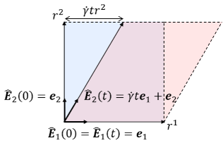
Figure 18: Schematic diagram of the oblique coordinate system. Here $\hat{\bm{E}}_{1}$ and $\hat{\bm{E}}_{2}$, and $\bm{e}_{1}$ and $\bm{e}_{2}$ are the basis vectors in the oblique system and those in the static Cartesian system, respectively; and $r^{1}$ and $r^{2}$ are the components of the position vector in the Cartesian system. The Cartesian system and the initial oblique system coincide (blue square). At $t>0$, the oblique system is sheared (pink parallelogram) by the strain of $\dot{\gamma}t$, where $\dot{\gamma}$ is the applied shear rate. The region of the oblique system outside the initial square (right triangle) can be periodically transformed back into the square (left triangle).

The periodicity in the governing equations can also be achieved by only the coordinate transformation (Eqs. (30)-(33)) with the orthogonal basis system (Rogallo, 1981; Onuki, 1997) without using the oblique dual-basis system. This single-basis formalism has the advantage that the tensorial representation for an equation is expressed uniquely but has the disadvantage that a spatial differential operator includes the cross oblique term explicitly. In contrast, the dual-basis formalism adopted in our method has the advantage that the forms of differential operators and governing equations in the oblique coordinate system are almost the same as that in the orthogonal system, as explained in Sec. A.2, although these forms have dual (covariant and contravariant) expressions. This simple expression of the governing equations in the coordinate system is preferable for a convenient implementation of the practical simulation code.

A.2 Governing equations in the oblique coordinate system

The tensorial component representation of the fluid momentum equation on the general coordinate system (Luo & Bewley, 2004; Venturi, 2009; Molina et al., 2016) is

$$\frac{\delta\hat{u}^{\mu}}{\delta\hat{t}}=\rho^{-1}\hat{\nabla}_{\nu}\hat{\sigma}^{\nu\mu}+\hat{\phi}\hat{f}_{p}^{\mu}.$$ (47)

The left-hand side of Eq. (47) is the intrinsic time derivative in the general coordinate system,

$$\frac{\delta\hat{A}^{\mu}}{\delta\hat{t}}\equiv\frac{\partial\hat{A}^{\mu}}{\partial\hat{t}}+(\hat{u}^{\nu}-\hat{U}^{\nu})\hat{\nabla}_{\nu}\hat{A}^{\mu}+\hat{A}^{\nu}\hat{\nabla}_{\nu}\hat{U}^{\mu},$$ (48)

where $\hat{U}^{\mu}\equiv-\partial\hat{r}^{\mu}/\partial t$ is the moving velocity of the coordinate and for simple shear flow $\bm{U}=\dot{\gamma}(t)r^{2}\bm{e}_{1}=\dot{\gamma}(t)\hat{r}^{2}\hat{\ bm{E}}_{1}$. Since $\hat{A}^{\mu}$ is defined in the moving system, the advection in the second term in Eq. (48) is by the relative velocity to the coordinate flow. The last term in Eq. (48) arises from the affine deformation caused by the coordinate flow. Introducing the relative fluid velocity to the coordinate flow $\bm{\xi}=\bm{u}-\bm{U}$, Eq. (47) becomes

$$(\hat{\partial}_{\hat{t}}+\hat{\xi}^{\nu}\hat{\nabla}_{\nu})\hat{\xi}^{\mu}=\rho^{-1}\hat{\nabla}_{\nu}\hat{\sigma}^{\nu\mu}+\hat{\phi}\hat{f}_{p}^{\mu}-2\dot{\gamma}(t)\hat{\xi}^{2}\delta^{\mu,1},$$ (49)

with the incompressibility condition $\hat{\nabla}_{\mu}\hat{\xi}^{\mu}=0$, where $\hat{\partial}_{\hat{t}}\equiv\partial/\partial\hat{t}|_{\hat{r}^{\mu}}=\partial/\partial t|_{r^{\mu}}+\dot{\gamma}(t)r^{2}\partial/\partial r^{1}$. The last term in Eq. (49) arises from the spatial gradient of the coordinate flow. Since this equation does not explicitly depend on the coordinate components $\hat{r}^{\mu}$, periodic boundary conditions can be assigned to Eq. (49), and hence Eq. (49) can be solved by a spectral method (Rogallo, 1981; Canuto et al., 1988). The stress tensor gradient in a Newtonian fluid is obtained as

$$\hat{\nabla}_{\nu}\hat{\sigma}_{n}^{\nu\mu}=-G^{\nu\mu}\hat{\nabla}_{\nu}\hat{p}+\eta_{s}G^{\nu\gamma}\hat{\nabla}_{\nu}\hat{\nabla}_{\gamma}\hat{\xi}^{\mu}.$$ (50)

In a viscoelastic fluid, the polymer stress gradient term $\hat{\nabla}_{\nu}\hat{\sigma}_{p}^{\nu\mu}$ is considered in addition to Eq. (50). In our method, the tensorial expression for the constitutive equation of the polymer stress is additionally introduced in a manner consistent with the previous Newtonian formulation (Molina et al., 2016).

The intrinsic time derivative for conformation tensor $\bm{C}=\hat{C}^{\mu\nu}\hat{\bm{E}}_{\mu}\hat{\bm{E}}_{\nu}$, which is represented by its second-rank contravariant tensor, is expressed as (Venturi, 2009)

$$\frac{\delta\hat{C}^{\mu\nu}}{\delta\hat{t}}\equiv\frac{\partial\hat{C}^{\mu\nu}}{\partial\hat{t}}+(\hat{u}^{\gamma}-\hat{U}^{\gamma})\hat{\nabla}_{\gamma}\hat{C}^{\mu\nu}+\hat{C}^{\mu\gamma}\hat{\nabla}_{\gamma}\hat{U}^{\nu}+\hat{C}^{\gamma\nu}\hat{\nabla}_{\gamma}\hat{U}^{\mu},$$ (51)

and the upper-convected time derivative is expressed by

$$\frac{d_{c}\hat{C}^{\mu\nu}}{d\hat{t}}\equiv\frac{\delta\hat{C}^{\mu\nu}}{\delta\hat{t}}-\hat{C}^{\gamma\nu}\hat{\nabla}_{\gamma}\hat{u}^{\mu}-\hat{C}^{\mu\gamma}\hat{\nabla}_{\gamma}\hat{u}^{\nu}.$$ (52)

Substituting Eq. (51) into Eq. (52), one obtains

$$\frac{d_{c}\hat{C}^{\mu\nu}}{d\hat{t}}=\frac{\partial\hat{C}^{\mu\nu}}{\partial\hat{t}}+\hat{\xi}^{\gamma}\hat{\nabla}_{\gamma}\hat{C}^{\mu\nu}-\hat{C}^{\mu\gamma}\hat{\nabla}_{\gamma}\hat{\xi}^{\nu}-\hat{C}^{\gamma\nu}\hat{\nabla}_{\gamma}\hat{\xi}^{\mu}.$$ (53)

By using Eq. (53), the single-mode Oldroyd-B constitutive equation in the general coordinate system is represented as

$$\frac{\partial\hat{C}^{\mu\nu}}{\partial\hat{t}}+\hat{\xi}^{\gamma}\hat{\nabla}_{\gamma}\hat{C}^{\mu\nu}=\hat{C}^{\mu\gamma}\hat{\nabla}_{\gamma}\hat{\xi}^{\nu}+\hat{C}^{\gamma\nu}\hat{\nabla}_{\gamma}\hat{\xi}^{\mu}-\frac{1}{\lambda}\left(\hat{C}^{\mu\nu}-G^{\mu\nu}\right),$$ (54)

$$\hat{\sigma}_{p}^{\mu\nu}=\frac{\eta_{p}}{\lambda}\left(\hat{C}^{\mu\nu}-G^{\mu\nu}\right).$$ (55)

Here, again, Eq. (54) is independent of the coordinate components and has the same form as that in the orthogonal coordinate system. Therefore, periodic boundary conditions can be assigned to Eq. (54).

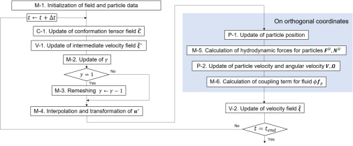
Figure 19: Flow chart of the main calculation procedure over one time step.

Appendix B Numerical implementation

B.1 Time-stepping algorithm for the coupling between fluid and particles

A flow chart showing the calculation procedure for one time step calculations is shown in Fig. 19. The couplings between the flow and conformation and between the fluid and particles are established in the following explicit fractional step approach. Throughout the evolution process, field variables are converted from real space to wavenumber space and vice versa as necessary. In this section, continuum variables in the Fourier space are denoted by the subscript $\bm{k}$, where $\bm{k}$ represents the wavenumber vector. The discretized $n$-th time step is indicated by the superscript of a variable as $(\cdot)^{n}$. Here, the constitutive equation is a single-mode Oldroyd-B model to ease explanation, and the extension to the multi-mode constitutive equations is straightforward. The calculation proceeds according to the following procedure.

1. Initialization of variables (M-1). Starting with the coordinate strain $\gamma=0$, the field variables are initialized as $\bm{u}=\bm{\xi}=\bm{0},\bm{C}=\bm{I}$ at $t=0$ over the entire domain. Correspondingly, the translational and angular velocities of the particles are set to zero. For a many-particle system, the positions of the particles are randomly generated to keep the distance between particle surfaces at least $2\Delta$, where $\Delta$ is the grid size.

2. Update of the conformation tensor field (C-1). The conformation tensor $\hat{\bm{C}}$ is updated to the next time step by integrating Eq. (54) or Eq. (85) over time to obtain the polymer stress field. As mentioned in Sec. II.2, the small error of $\hat{\bm{C}}$ accumulates in the inner particle region according to the time evolution. This error can be eliminated by resetting $\hat{\bm{C}}=\bm{G}$ over the $\hat{\phi}=1$ region if necessary. In this study, this reset operation is safely omitted because the error is sufficiently small.

3. Update of the intermediate velocity field (V-1). Equation (49) without the $\hat{\phi}\hat{\bm{f}}_{p}$ term is time-integrated to obtain an intermediate velocity field $\hat{\bm{\xi}}^{*}$. In this step, the fluid stress, i.e., the solvent and polymer stresses, are considered, and the solid–fluid coupling is not considered.

4. Update of the shear strain (M-2). After the field calculations, the shear strain is updated: $\gamma^{n+1}=\gamma^{n}+\dot{\gamma}\Delta t$, where $\Delta t$ is the time increment. This corresponds to the deformation of the oblique coordinate system. In this step, if the apparent shear strain equals the threshold value $\gamma_{\rm{th}}$, the remeshing process is conducted. In this study, $\gamma_{\rm{th}}=1$.

5. Remeshing (M-3). Practically, as time evolves, the oblique mesh is gradually distorted, which can lead to a decrease in accuracy. To continue the simulation as the strain increases infinitely while maintaining accuracy, the strained oblique coordinates should be reset to a less strained state or to the static Cartesian coordinates at some finite shear strain (Rogallo, 1981). In this study, the oblique coordinate system is reset to the orthogonal Cartesian coordinate system when $\gamma$ reaches $\gamma_{\rm{th}}=1$. First, the shear strain of the oblique system is reset as $\gamma\leftarrow\gamma-\gamma_{\rm{th}}$. Then, the field variables $\hat{\bm{\xi}}^{*},\hat{\bm{C}}$ on the oblique grid outside of the initial orthogonal grid are remapped through the periodic boundary in the flow direction. Simultaneously, the components of the variables in the oblique coordinate system are transformed to those in the reset coordinate system by the transformation matrix. Correspondingly, the metric tensor (Eq. (46)) and the norm of the wavenumber vector in the spectral scheme, $\hat{\bm{k}}\cdot\hat{\bm{k}}$, are updated. The norm of wavenumber vector in the wavenumber space corresponds to the Laplacian operator in real space, i.e. $G^{\mu\nu}\hat{\nabla}_{\mu}\hat{\nabla}_{\nu}\Leftrightarrow-G^{\mu\nu}\hat{k}_{\mu}\hat{k}_{\nu}=-\hat{\bm{k}}\cdot\hat{\bm{k}}$, and then

   $$\hat{\bm{k}}\cdot\hat{\bm{k}}=\hat{k}_{1}^{2}+(\hat{k}_{2}-\gamma\hat{k}_{1})^{2}+\hat{k}_{3}^{2},$$ (56)

   where $\hat{k}_{i}$ is the $i$-th component of the covariant wavenumber vector in the oblique coordinate system.

6. Interpolation and transformation of the intermediate velocity field (M-4). To simplify the reconstruction of the $\phi$ field based on particle positions, the coupling between the fluid and particle is treated on the usual static orthogonal coordinate system. The grid points in the oblique coordinate system do not always coincide with those in the static orthogonal coordinate system. Therefore, the intermediate velocity field $\hat{\bm{\xi}}^{*}$ on the oblique grids should be interpolated to the static orthogonal grids. This is done by using a periodic cubic spline interpolation (Molina et al., 2016). After the interpolation, the oblique-basis components of $\hat{\bm{\xi}}^{*}$ are transformed to those in Cartesian basis. In this step, the absolute velocity field $\bm{u}^{*}$ is constructed using the transformed $\bm{\xi^{*}}$ and the base flow $\dot{\gamma}r^{2}\bm{e}_{1}$:

   $$\bm{u}^{*}=(\dot{\gamma}r^{2}\delta^{\mu,1}+\Lambda^{\mu}_{\;\;\nu}\hat{\xi}^{\nu*})\bm{e}_{\mu}.$$ (57)

7. Update of the particle position (P-1). Hereafter, the calculation is conducted in the orthogonal coordinate system (blue block in Fig. 19). Using the particle velocity at the previous time step $\bm{V}^{n}$, the position of the $i$-th particle is updated:

   $$\bm{R}_{i}^{n+1}=\bm{R}_{i}^{n}+\int_{t^{n}}^{t^{n+1}}\bm{V}_{i}^{n}dt.$$ (58)

   In this step, if the updated particle position crosses the top and bottom boundaries, the position and velocity of the particle are modified according to the Lees–Edwards boundary conditions (Lees & Edwards, 1972; Kobayashi & Yamamoto, 2011; Molina et al., 2016). In this time, the $\phi$ field is also updated by using the new particle positions consistent with Lees–Edwards boundary conditions. Then, the intermediate particle velocity field $\bm{u}_{p}^{*}$ is calculated:

   $$\phi^{n+1}\bm{u}_{p}^{*}=\sum_{i}\phi_{i}^{n+1}\left[\bm{V}_{i}^{n}+\bm{\Omega}_{i}^{n}\times\bm{r}_{i}^{n+1}\right],$$ (59)

   where $\bm{r}_{i}=\bm{r}-\bm{R_{i}}$. This corresponds to the mapping of the Lagrangian particle velocity on the Euler velocity field.

8. Calculation of hydrodynamic forces acting on particles (M-5). The hydrodynamic force and torque exerted on the particles $\bm{F}^{H}$ and $\bm{N}^{H}$ are calculated by the change in momentum in the particle domain:

   $$\int_{t^{n}}^{t^{n+1}}\bm{F}_{i}^{H}dt =\int\rho\phi_{i}^{n+1}(\bm{u}^{*}-\bm{u}_{p}^{*})d\bm{r},$$ (60)

   $$\int_{t^{n}}^{t^{n+1}}\bm{N}_{i}^{H}dt =\int\bm{r}_{i}^{n+1}\times\rho\phi_{i}^{n+1}(\bm{u}^{*}-\bm{u}_{p}^{*})d\bm{r}.$$ (61)

9. Update of the particle velocity and angular velocity (P-2). Using Eqs. (60) and (61), the particle velocities are updated as

   $$\bm{V}_{i}^{n+1} =\bm{V}_{i}^{n}+\frac{1}{M_{i}}\int_{t^{n}}^{t^{n+1}}\left[\bm{F}_{i}^{H}+\bm{F}_{i}^{C}\right]dt,$$ (62)

   $$\bm{\Omega}_{i}^{n+1} =\bm{\Omega}_{i}^{n}+\bm{I}_{p,i}^{-1}\cdot\int_{t^{n}}^{t^{n+1}}\bm{N}_{i}^{H}dt.$$ (63)

   In this study, for the inter-particle force $\bm{F}^{C}$, the soft-core (truncated Lenard–Jones) potential, which produces the short-range repulsive force, is adopted:

   $$\bm{F}^{C}_{i}(\bm{R}) =-\sum_{j\neq i}^{N}F_{\rm{soft}}(r_{ij})\frac{\bm{r}_{ij}}{|\bm{r}_{ij}|},$$ (64)

   $$F_{\rm{soft}}(r_{ij}) =-\left(\frac{\partial U_{\rm{soft}}}{\partial r}\right)_{r=r_{ij}},$$ (65)

   $$U_{\rm{soft}}(r) =\begin{cases}4\epsilon\left[\left(\frac{2a}{r}\right)^{36}-\left(\frac{2a}{r}\right)^{18}\right]+\epsilon&(r<r_{c})\\ 0&(r\geq r_{c}),\end{cases}$$ (66)

   where $\bm{r}_{ij}=\bm{R}_{j}-\bm{R}_{i}$ is the distance vector from the $i$-th particle to the $j$-th particle and $r_{c}=2^{1/18}(2a)$. Vector $\bm{r}_{ij}$ is modified according to periodic boundary conditions if necessary. This potential force is simply applied to avoid particle overlap. The force parameter $\epsilon$, which tunes the interaction strength, is set at $\epsilon/(\eta_{0}\dot{\gamma}a^{3})=0.561$ in all many-particle calculations in this study. Under denser particle concentration conditions, where the particle collisions and/or friction and its contribution to the total stress can become significant, more realistic modelling of inter-particle force may be required.

10. Calculation of the coupling term for fluid (M-6). Now that both the positions and velocities of particles have been updated, the final particle velocity field $\bm{u}_{p}$ is obtained as

    $$\phi^{n+1}\bm{u}_{p}^{n+1}=\sum_{i}\phi_{i}^{n+1}\left[\bm{V}_{i}^{n+1}+\bm{\Omega}_{i}^{n+1}\times\bm{r}_{i}^{n+1}\right].$$ (67)

    Then, the body force $\phi\bm{f}_{p}$ is calculated as

    $$\int_{t^{n}}^{t^{n+1}}\phi\bm{f}_{p}(\bm{x},t)dt=\phi^{n+1}(\bm{u}_{p}^{n+1}-\bm{u}^{*}).$$ (68)

    To calculate the stresslet (Eq. (19)), Eq. (68) is further transformed as

    $$\int_{t^{n}}^{t^{n+1}}\phi\bm{f}_{p}dt=\phi^{n+1}(\bm{u}_{p}^{n+1}-\bm{u}^{*}_{p})-\phi^{n+1}(\bm{u}^{*}-\bm{u}_{p}^{*}).$$ (69)

    The first term on the RHS is expressed by the changes in particle velocity $\Delta\bm{V}_{i}=\bm{V}_{i}^{n+1}-\bm{V}_{i}^{n}$ from Eq. (62) and in angular velocity $\Delta\bm{\Omega}_{i}=\bm{\Omega}_{i}^{n+1}-\bm{\Omega}_{i}^{n}$ from Eq. (63), as

    $$\phi^{n+1}(\bm{u}_{p}^{n+1}-\bm{u}_{p}^{*}) =\sum_{i}\phi_{i}^{n+1}[\Delta\bm{V}_{i}^{H}+\Delta\bm{\Omega}_{i}^{H}\times\bm{r}_{i}^{n+1}]$$

    $$~{}~{}~{}~{}+\sum_{i}\phi_{i}^{n+1}\Delta\bm{V}_{i}^{C},$$ (70)

    where $\Delta\bm{V}_{i}^{H},\,\Delta\bm{\Omega}_{i}^{H}$, and $\Delta\bm{V}_{i}^{C}$ are the updates by the hydrodynamic forces $\bm{F}_{i}^{H}$ and $\bm{N}_{i}^{H}$ and the inter-particle force $\bm{F}_{i}^{C}$, respectively. Therefore, $\phi\bm{f}_{p}$ can be decomposed into the individual contributions from the hydrodynamic interactions $\phi\bm{f}_{p}^{H}$ and direct inter-particle interactions $\phi\bm{f}_{p}^{C}$, as $\phi\bm{f}_{p}=\phi\bm{f}_{p}^{H}+\phi\bm{f}_{p}^{C}$. The individual contributions of the body force are expressed to first order in time as

    $$\phi\bm{f}_{p}^{H}\Delta t =\sum_{i}\phi_{i}^{n+1}[\Delta\bm{V}_{i}^{H}+\Delta\bm{\Omega}_{i}^{H}\times\bm{r}_{i}^{n+1}]-\phi^{n+1}(\bm{u}^{*}-\bm{u}_{p}^{*}),$$ (71)

    $$\phi\bm{f}_{p}^{C}\Delta t =\sum_{i}\phi_{i}^{n+1}\Delta\bm{V}_{i}^{C}.$$ (72)

    In the calculation of the stresslet contribution from $\phi\bm{f}_{p}^{C}$, the direct virial expression was used instead of Eq. (72) for computational efficiency (Molina et al., 2016):

    $$\bm{S}^{C}=-\frac{1}{N}\int_{D_{V}}\bm{r}\rho\phi\bm{f}_{p}^{C}d\bm{r}=-\frac{1}{N}\sum_{i<j}\bm{r}_{ij}\bm{F}_{ij}^{C},$$ (73)

    where $\bm{F}_{ij}^{C}$ is the inter-particle force on the $i$-th particle due to the $j$-th particle. In this study, for conditions up to $\phi_{p}=0.1$ and $\rm{Wi}=2.5$, the contribution of $S_{12}^{C}$ to the total stresslet $S_{12}$ is small compared to the hydrodynamic contributions ($\langle S_{12}^{C}\rangle/\langle S_{12}\rangle<0.05$ at $\phi_{p}=0.1$).

11. Update of the velocity field (V-2). Finally, the integrated body force $\phi\bm{f}_{p}$ is remapped and transformed from the orthogonal coordinate system to the oblique coordinate system and added to the intermediate velocity field $\hat{\bm{\xi}}^{*}$:

    $$\hat{\bm{\xi}}^{n+1}=\hat{\bm{\xi}}^{*}+\widehat{\left[\int_{t^{n}}^{t^{n+1}}\phi\bm{f}_{p}ds\right]}.$$ (74)

    At this stage, incompressibility is assigned in the Fourier space,

    $$\hat{\bm{\xi}}_{\bm{k}}\leftarrow\hat{\bm{\xi}}_{\bm{k}}-\frac{(\hat{\xi}_{\bm{k}}\cdot\hat{\bm{k}})}{\hat{\bm{k}}\cdot\hat{\bm{k}}}\hat{\bm{k}}.$$ (75)

    This solenoidal projection is also adopted after calculating $\hat{\bm{\xi}}^{*}$ (V-1).

The described fractional steps are repeated until the calculated time reaches the target final time. Further information about the time-stepping algorithm is detailed in previous work (Nakayama et al., 2008; Molina et al., 2016).

B.2 Spatial discretization and time integral scheme

Since the periodic boundary conditions are assigned in each direction, the continuum variables such as $\hat{\bm{\xi}}$, and $\hat{\bm{C}}$ are Fourier-transformed. In real space, the continuum variables are collocated on the equispaced mesh point with spacing $\Delta$. Spatial derivatives are calculated in Fourier space while the second-order terms like the advection term in Eq. (49) and (54) are calculated by a transformation method (Orszag, 1969).

For the integration of $\hat{\bm{\xi}}_{\bm{k}}$ over time, the exact linear part (ELP) method, which is preferred for solving stiff equations (Beylkin et al., 1998), is adopted, where the nonlinear part is discretized by the Euler method.

For the polymer constitutive equation, the explicit Euler method (first-order) is adopted. In this study, to evaluate a single-particle system that corresponds to very dilute suspensions ($\phi_{p}\sim 0.001$), the discretized Eq. (54) is solved directly. This naive implementation has been stable and accurate in such dilute conditions. However, at high $\phi_{p}$ and ${\rm Wi}$ conditions, the large growth rate of the polymer stress around the particles violates the positive definiteness of the conformation tensor, thus resulting in an inaccurate solution or divergence. Therefore, to evaluate a many-particle system that corresponds to semi-dilute suspensions ($0.025\leq\phi_{p}\leq 0.1$), the log-conformation formalism is used in which the time evolution equation of $\log\bm{C}$ rather than $\bm{C}$ is solved to guarantee the positive-definiteness of $\bm{C}$ (Fattal & Kupferman, 2004; Hulsen et al., 2005). A detailed description of the log-conformation formalism is provided in Appendix B.3.

The particle position is updated by discretizing Eq. (58) by the Euler method (first-order) at the first time step and the second-order Adams–Bashforth scheme later. In the update of the particle velocity (Eqs. (62) and (63)), the impulsive hydrodynamic force and torque are calculated by applying Eqs. (60) and (61), respectively, and the potential force $\bm{F}^{C}$ in Eq. (62) is discretized by the second-order Heun scheme because both particle positions at $t^{n}$ and $t^{n+1}$ are already obtained in that stage:

$$\frac{1}{M_{i}}\int_{t^{n}}^{t^{n+1}}\bm{F}_{i}^{C}ds=\frac{\Delta t}{2M_{i}}\left[\bm{F}_{i}^{C}(\bm{R}^{n+1})+\bm{F}_{i}^{C}(\bm{R}^{n})\right].$$ (76)

The time increment is determined based on the stability given by the fluid momentum diffusion: $\Delta t=\rho/\eta_{0}K_{\rm max}^{2}$ ($K_{\rm max}$ is the largest wavenumber in the spectral scheme). As proven in the code validations in Sec. III.1 and Appendix C, this choice is reasonable considering the conditions in this study.

B.3 Log-conformation-based constitutive equation for Oldroyd-B model

Because the conformation tensor $\bm{C}$ is real-symmetric and positive-definite, $\bm{C}$ can be diagonalized as

$$\bm{C}=\bm{R}\cdot\bm{\Lambda}\cdot\bm{R}^{T},$$ (77)

where $\bm{\Lambda}=\rm{diag}(\lambda_{1},\lambda_{2},\lambda_{3})$ and $\lambda_{i}>0\,(i=1,2,3)$ are the eigenvalues of $\bm{C}$, and $\bm{R}$ is the rotation matrix composed of the eigenvectors of $\bm{C}$. Here, the new tensor variable $\bm{\Psi}$ is introduced (Fattal & Kupferman, 2004) as

$$\bm{\Psi}=\bm{R}\cdot\bm{\Lambda}_{\Psi}\cdot\bm{R}^{T},$$ (78)

where $\bm{\Lambda}_{\Psi}=\rm{diag}(\ln\lambda_{1},\ln\lambda_{2},\ln\lambda_{3})=\ln\bm{\Lambda}$. From Eqs. (77) and (78),

$$\bm{C}=\bm{R}\cdot\exp(\bm{\Lambda}_{\Psi})\cdot\bm{R}^{T}.$$ (79)

Note that, when $\bm{C}$ is obtained through Eq. (79), $\bm{C}$ is strictly positive-definite by definition. Furthermore, utilizing the time evolution of $\bm{\Psi}$ instead of Eq. (4), the exponential growth in $\bm{C}$ is translated to the linear growth of $\bm{\Psi}$, which enables numerical stability in the time evolution. Specifically, the stretching in the principal axes of $\bm{C}$ by the velocity gradient tensor $\bm{\nabla}\bm{u}$ is extracted as

$$\bm{\nabla u} =\bm{R}\cdot\bm{M}\cdot\bm{R}^{T},$$ (80)

$$\bm{B} =\bm{R}\cdot{\rm diag}(M_{11},M_{22},M_{33})\cdot\bm{R}^{T},$$ (81)

where $\bm{B}$ is symmetric and commutes with $\bm{C}$ by definition.

The residual component $\bm{\nabla}\bm{u}-\bm{B}$ can be decomposed as

$$\bm{\nabla u}-\bm{B}=\bm{A}+\bm{C}^{-1}\cdot\bm{N},$$ (82)

with anti-symmetric tensors $\bm{A}$ and $\bm{N}$ (Fattal & Kupferman, 2004). Tensor $\bm{N}$ is proven to be irrelevant in the affine deformation of $\bm{C}$ by inserting Eq. (82) into the upper-convected time derivative of $\bm{C}$. On the other hand, $\bm{A}$ represents the rotation of the principal axes of $\bm{C}$. From the affine deformation of $\bm{C}$ in Eq. (4), the explicit expression of $\bm{A}$ in the frame of the principal axes of $\bm{C}$ is derived by Hulsen et al. (2005) as

$$A_{ij}=\frac{\lambda_{i}M_{ij}+\lambda_{j}M_{ji}}{\lambda_{i}-\lambda_{j}},~{}~{}i\neq j,~{}~{}\lambda_{i}\neq\lambda_{j},$$ (83)

(the summation convention is not applied here). When $\lambda_{i}=\lambda_{j}$, $A_{ij}$ is not uniquely determined in the decomposition of $\bm{\nabla u}$ in Eq. (82), but the affine deformation of $\bm{C}$ and $\bm{\Psi}$ by $\bm{\nabla u}$ is still well defined, which case is explained next.

By using these tensors, the governing equation of $\bm{\Psi}$ for the single-mode Oldroyd-B model is expressed as

$$\left(\frac{\partial}{\partial t}+\bm{u}\cdot\bm{\nabla}\right)\bm{\Psi} =-\bm{A}\cdot\bm{\Psi}+\bm{\Psi}\cdot\bm{A}+2\bm{B}$$

$$~{}~{}~{}~{}+\bm{R}\cdot\left[\frac{1}{\lambda}(\bm{\Lambda}^{-1}-\bm{I})\right]\cdot\bm{R}^{T}.$$ (84)

When $\lambda_{i}=\lambda_{j}$, the corotational terms including $A_{ij}$ are reduced as (in the frame of the principal axes of $\bm{C}$)

$$-A_{ij}\Psi_{jj}+\Psi_{ii}A_{ij} =\left(\ln\lambda_{i}-\ln\lambda_{j}\right)\frac{\lambda_{i}M_{ij}+\lambda_{j}M_{ji}}{\lambda_{i}-\lambda_{j}}$$

$$\to M_{ij}+M_{ji}=2D_{ij},$$

(the summation convention is not applied here). With this treatment, the evolution equation (B.3) of $\bm{\Psi}$ works safely even when $\lambda_{i}=\lambda_{j}$ happens.

In the initial conditions, $\bm{u}=\bm{0}$ over the entire domain leads to $\bm{A}=\bm{0}$ and $\bm{B}=\bm{D}$, and $\bm{C}=\bm{I}$ results in $\bm{R}=\bm{I},\bm{\Lambda}=\bm{I}$, and $\bm{\Psi}=\bm{0}$. The evolution of $\bm{\Psi}$ according to Eq. (B.3) is solved by numerical simulation; and $\bm{C}$ is calculated from $\bm{\Psi}$ via Eqs. (78) and (79). The contravariant tensor expression corresponding to Eq. (B.3) in the oblique coordinates is the following:

$$\begin{split}\left(\frac{\partial}{\partial\hat{t}}+\hat{\xi}^{\gamma}\hat{\nabla}_{\gamma}\right)\hat{\Psi}^{\mu\nu}=&-\dot{\gamma}\left(\hat{\Psi}^{\mu 2}\delta^{1,\nu}+\hat{\Psi}^{2\nu}\delta^{1,\mu}\right)-G_{\gamma\zeta}\hat{A}^{\mu\gamma}\hat{\Psi}^{\zeta\nu}+G_{\gamma\zeta}\hat{\Psi}^{\mu\gamma}\hat{A}^{\zeta\nu}+2\hat{B}^{\mu\nu}+\hat{R}^{\mu\gamma}\left[\frac{1}{\lambda}([\hat{\bm{\Lambda}}]^{-1}_{\gamma\zeta}-G_{\gamma\zeta})\right]\hat{R}^{\nu\zeta},\end{split}$$ (85)

where $[\hat{\bm{\Lambda}}]^{-1}_{\gamma\zeta}$ represents the covariant matrix component of $\hat{\bm{\Lambda}}^{-1}$, which is simply the matrix inverse of the contravariant matrix $\hat{\Lambda}^{\gamma\zeta}$; and $G_{\gamma\zeta}$ is the covariant metric tensor, which is defined as

$$G_{\gamma\zeta}\equiv\hat{\bm{E}}_{\gamma}\cdot\hat{\bm{E}}_{\zeta}=\left(\begin{array}[]{ccc}1&\gamma(t)&0\\ \gamma(t)&1+\gamma^{2}(t)&0\\ 0&0&1\end{array}\right).$$ (89)

Note that, in the oblique coordinates, there is an additional term originating from the moving coordinates (the first term on RHS of Eq. (85)). Since Eq. (85) does not explicitly depend on the coordinate variables, it can be discretized by a spectral method.

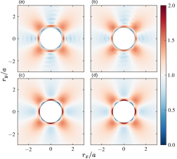
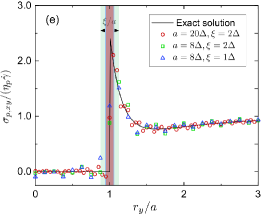
Figure 20: Mesh resolution dependence of polymer shear stress distributions near the particle. In panels (a-d) the polymer shear stress normalized by $\eta_{p}\dot{\gamma}$ on the shear plane through the center of the particle is drawn by color contour in (a-d) for $(a/\Delta,\xi/\Delta)=(8,2),\,(8,1)$, and $(20,2)$ and for the analytical solution, respectively. The dotted lines around the particles for the DNS results in panels (a-c) denote the radial location of $a+\xi/2$. In panel (e), the normalized polymer shear stress along the line from the particle center to the shear gradient direction $y$ is drawn: the exact solution (analytical) of $\bm{\sigma}_{p}/(\eta_{p}\dot{\gamma})\approx 2\tilde{\bm{D}}-2{\rm Wi}\tilde{\bm{D}}_{(2)}$ at ${\rm Wi}\to 0$ (solid line), the results for $(a/\Delta,\xi/\Delta)=(20,\,2)$ (red), $(8,2)$ (green), and $(8,1)$ (blue), respectively. In panel (e), the interface region indicated by $0<\phi<1$ at around $r_{y}/a=1$ with thickeness $\xi$ is colored in the same manner as that for the symbols.

Appendix C Validations of the developed method

C.1 Polymer stress around a single particle

To test the validity of the developed method, a single-particle system is set up where a neutrally buoyant spherical particle is suspended in a sheared Oldroyd-B fluid (Fig. 1(a)). The cubic domain with a box length of $L$ is sufficiently large compared to the size of the particle used to represent the dilute particle system. Hereafter, for simplicity, the directions of the Cartesian coordinate basis vectors are denoted by $x,y,$ and $z$ instead of the $1,2,$ and $3$ notation used in Appendices A and B, where $x,y$, and $z$ indicate the flow, velocity-gradient, and vorticity directions, respectively. As shown in Fig. 1(a), because the particle is located at the center of simple shear flow, the net translational hydrodynamic force acting on the particle $\bm{F}^{H}$ vanishes while the hydrodynamic torque $\bm{N}^{H}$ rotates the particle.

A flow condition is considered in the $\beta\to 1$, small-$\rm{Wi}$ and small-$\rm{Re}$ limit where an analytical solution is available. In this limit, the flow pattern is minimally affected by polymer stress, which is expressed analytically (Lin et al., 1970; Mikulencak & Morris, 2004). Furthermore, when $\rm{Wi}\ll 1$, the polymer stress distribution is approximated by the second-order fluid (SOF) theory; $\bm{\sigma}_{p}=2\eta_{p}\bm{D}+4(\Psi_{1}+\Psi_{2})\bm{D}\cdot\bm{D}-\P si_{1}(\bm{D}_{(2)}+4\bm{D}\cdot\bm{D})$, where $\bm{D}_{(2)}$ is the upper-convected derivative of $\bm{D}$ (Bird et al., 1987). Considering an Oldroyd-B fluid ($\Psi_{1}=2\eta_{p}\lambda,\,\Psi_{2}=0$), the normalized polymer stress in the SOF limit is expressed as $\bm{\sigma}_{p}/(\eta_{p}\dot{\gamma})=2\tilde{\bm{D}}-2{\rm Wi}\tilde{\bm{D}}_{(2)}$. Here, $\beta=0.99,\rm{Wi}=0.001$, and $\rm{Re}=0.0142$. In this situation, the normalized polymer stress is approximated by $\bm{\sigma}_{p}/(\eta_{p}\dot{\gamma})\approx 2\tilde{\bm{D}}$.

Different mesh resolutions of the particle interface are examined: $(a/\Delta,\xi/\Delta)=(8,2),(8,1),$ and $(20,2)$. At first, the overall trend of the polymer shear stress ($\sigma_{p,xy}$) distribution is similar for different resolutions (Fig. 20(a-c)) and the analytical solution ( Fig. 20(d)). The only difference is that small $\sigma_{p,xy}$ oscillation is observed in the numerical solutions. When comparing the results for $a=8\Delta$ and $\xi=2\Delta$ (Fig. 20(a)) with that for $a=20\Delta$ and $\xi=2\Delta$ (Fig. 20(c)), it is clear that as $a/\Delta$ increases, the wavenumber of the small ripple in $\sigma_{p,xy}$ increases, but its amplitude decreases. This is due to the slow convergence of the Fourier series caused by the discontinuous change in $\sigma_{p,xy}$ at the solid–liquid interface. This artifact is a partly unavoidable intrinsic property of the spectral method. Regarding the interface thickness, when comparing the results for $a=8\Delta$ and $\xi=2\Delta$ (Fig. 20(a)) with that for $a=8\Delta$ and $\xi=\Delta$ (Fig. 20(b)), no significant difference in the overall trend is observed. However, when $\xi=\Delta$, the distribution of ${\sigma}_{p,xy}$ near the interface is somewhat blurred, which is caused by the decrease in the number of mesh points that support the interface region.

For a detailed evaluation, a one-dimensional profile of the polymer shear stress in the velocity-gradient direction from the particle center is shown in Fig. 20(e). The steep increase in $\sigma_{p,xy}$ near the particle surface is reasonably reproduced as the mesh resolution increases, though the peak in $\sigma_{p,xy}$ is somewhat smeared due to the limited mesh points in the interface domain. Hereafter, considering a balance between the accuracy of the numerical solution and the required computational cost, the particle radius is set to $a=8\Delta$ and the interface thickness to $\xi=2\Delta$. As seen in Appendix C.2 and Sec. III, this resolution is sufficiently valid for the problems investigated in this study.

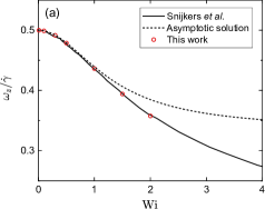
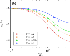
Figure 21: The $\rm{Wi}$ dependence of the normalized particle angular velocity $\omega_{z}/\dot{\gamma}$. (a) The result of this work (red circles) compared with a previous numerical result (solid line) (Snijkers et al., 2009) and the asymptotic solution (dashed line) (Housiadas & Tanner, 2011a, b, 2018)

at $\beta=0.615$. (b) The $\beta$ dependence of $\omega_{z}/\dot{\gamma}$ for: $\beta=0.2$ (red circles), $0.5$ (orange squares), $0.615$ (green triangles), and $0.8$ (blue diamonds). The lines correspond to predictions of the asymptotic solution.

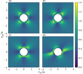
Figure 22: The $\rm{Wi}$ dependence of the normalized energy dissipation around a particle at $\beta=0.5$: (a)(b) $\rm{Wi}=0.1$ and (c)(d) $\rm{Wi}=1.0$. Panels (a)(c) and (b)(d) show the distributions of viscous dissipation $\Phi_{\rm s}/(\eta_{0}\dot{\gamma}^{2})$ and polymer dissipation $\Phi_{\rm p}/(\eta_{0}\dot{\gamma}^{2})$, respectively. The dotted lines around particles show the radial location of $a+\xi/2$.

C.2 Rotation of a particle under simple shear flow

Under simple shear in Stokes flow, as is well known, a suspended particle in a Newtonian medium rotates with an angular velocity that is half of the applied shear rate; $\omega_{z}/\dot{\gamma}=0.5$, where $\omega_{z}$ is the particle angular velocity in the vorticity direction. However, in viscoelastic fluids, this relative rotational speed decreases with increasing $\rm{Wi}$ (Snijkers et al., 2009, 2011). D’Avino et al. (2008) and Snijkers et al. (2009, 2011) conducted numerical evaluation for this phenomenon using a finite element method (FEM) and surface-conforming mesh, reproducing the experimental rotational slowdown data with DNS. They observed that the distribution of local torque and pressure on the particle surface becomes asymmetrical with $\rm{Wi}$. However, the physics of slowdown has not been elucidated. This result is often referred to as the benchmark problem for a newly developed numerical scheme of viscoelastic suspensions (Ji et al., 2011; Yang et al., 2016; Vázquez-Quesada & Ellero, 2017; Fernandes et al., 2019). To validate the method developed in this work, the angular velocity of a particle in an Oldroyd-B fluid is evaluated at the same numerical conditions previously reported (Snijkers et al., 2009); however, no walls are used in this study. The numerical setup is the same as that in Sec. III.1.

Figures. 21(a) and (b) show the $\beta$ and $\rm{Wi}$ dependence of the normalized particle angular velocity $\omega_{z}/\dot{\gamma}$. To compare with the previous numerical result, Fig. 21(a) shows the result at $\beta=0.615$. As $\rm{Wi}$ increases, $\omega_{z}/\dot{\gamma}$ decreases. At $\rm{Wi}\lesssim 1$, the result converges with the theoretical prediction up to $O(\rm{Wi}^{4})$ made using asymptotic methods (Housiadas & Tanner, 2011a, b, 2018): $\omega_{z}/\dot{\gamma}=1/2-(1-\beta)\rm{Wi}^{2}/[4(1-4\rm{Wi}^{2}\tilde{\Omega}_{4})]$, where $\tilde{\Omega}_{4}$ is the coefficient of the $(1-\beta)\rm{Wi}^{4}$ term in the series solution. At $\rm{Wi}\gtrsim 1$, the asymptotic prediction starts to overestimate $\omega_{z}/\dot{\gamma}$. In this region, the result agrees reasonably well with the previous FEM result (Snijkers et al., 2009). Fig. 21(b) shows the $\beta$ dependence of $\omega_{z}/\dot{\gamma}$. As $\beta$ decreases, which corresponds to an increase in the polymer stress contribution, the negative slope of $\omega_{z}/\dot{\gamma}$ increases. This trend is consistent with the asymptotic predictions shown in Fig. 21(b).

The slowdown of rotation with increasing $\rm{Wi}$ and/or $1-\beta$ suggests that the energy partition from external work to elastic energy increases. Fig. 22 shows the normalized energy dissipation rate around the particle on the shear plane through the particle center at $\beta=0.5$ and $\rm{Wi}=0.1$ and $1.0$. The dissipation rate is decomposed into viscous ($\Phi_{\rm s}$) and elastic ($\Phi_{\rm p}$) contributions (Vázquez-Quesada et al., 2019) as $\Phi_{\rm{t}}=\Phi_{\rm{s}}+\Phi_{\rm{p}}$:

$$\Phi_{\rm s} =2\eta_{s}\bm{D}:\bm{D},$$ (90)

$$\Phi_{\rm p} =\frac{\eta_{p}}{2\lambda^{2}}\left({\rm tr}\bm{C}+{\rm tr}\bm{C}^{-1}-6\right).$$ (91)

At $\rm{Wi}=0.1$, $\Phi_{\rm s}$ (Fig. 22(a)) and $\Phi_{\rm p}$ (Fig. 22(b)) present similar distributions. Since $\bm{\sigma}_{p}=(\eta_{p}/\lambda)(\bm{C}-\bm{I})\to 2\eta_{p}\bm{D}$ at $\rm{Wi}\to 0$, $\Phi_{\rm p}$ is reduced to $2\eta_{p}\bm{D}:\bm{D}$, which is proportional to $\Phi_{\rm s}$. In contrast, at $\rm{Wi}=1.0$, $\Phi_{\rm s}$ and $\Phi_{\rm p}$ develop differently; the high-$\Phi_{\rm p}$ region expands, whereas $\Phi_{\rm s}$ does not change much in comparison to the $\rm{Wi}=0.1$ case. The distribution of $\Phi_{\rm p}$ expands towards the shear-flow direction and high-$\Phi_{\rm p}$ grows near the equator of the particle (Fig. 22(d)), thus clearly showing an increase in the fraction of elastic energy dissipation at high $\rm{Wi}$. Particle rotation is caused by viscous stress. An increase in elastic energy leads to a decrease in the relative fraction of viscous dissipation. As a result, the angular velocity of the particle in the viscoelastic medium decreases in comparison with that in viscous media. This slowdown of the particle rotation is enhanced with $\rm{Wi}$ and $1-\beta$.

In this section, the agreement between the numerical results of this work and the previously reported numerical and theoretical results verifies that the presented numerical scheme can successfully capture the dynamic coupling between particles and a viscoelastic fluid.

References

- Alghalibi et al. (2018) Alghalibi, Dhiya, Lashgari, Iman, Brandt, Luca & Hormozi, Sarah 2018 Interface-resolved simulations of particle suspensions in Newtonian, shear thinning and shear thickening carrier fluids. Journal of Fluid Mechanics 852, 329–357, arXiv: 1711.04195.
- Batchelor & Green (1972) Batchelor, GK & Green, JT 1972 The determination of the bulk stress in a suspension of spherical particles to order c2. Journal of Fluid Mechanics 56 (3), 401–427.
- Beylkin et al. (1998) Beylkin, Gregory, Keiser, James M. & Vozovoi, Lev 1998 A new class of time discretization schemes for the solution of nonlinear PDEs. Journal of Computational Physics 147 (2), 362–387.
- Bird et al. (1987) Bird, Robert Byron, Curtiss, Charles F, Armstrong, Robert C & Hassager, Ole 1987 Dynamics of Polymeric Liquids, Volume 2: Kinetic Theory. Wiley.
- Boger (1977) Boger, D. V. 1977 A highly elastic constant-viscosity fluid. Journal of Non-Newtonian Fluid Mechanics 3 (1), 87–91.
- Canuto et al. (1988) Canuto, Claudio, Hussaini, M. Yousuff, Quarteroni, Alfio & Zang, Thomas A. 1988 Spectral Methods in Fluid Dynamics. Berlin, Heidelberg: Springer Berlin Heidelberg.
- Chateau et al. (2008) Chateau, Xavier, Ovarlez, Guillaume & Trung, Kien Luu 2008 Homogenization approach to the behavior of suspensions of noncolloidal particles in yield stress fluids. Journal of Rheology 52 (2), 489–506, arXiv: 1006.2293.
- Dai et al. (2014) Dai, Shao-Cong, Qi, Fuzhong & Tanner, Roger I. 2014 Viscometric functions of concentrated non-colloidal suspensions of spheres in a viscoelastic matrix. Journal of Rheology 58 (1), 183–198.
- D’Avino et al. (2013) D’Avino, G., Greco, F., Hulsen, M. A. & Maffettone, P. L. 2013 Rheology of viscoelastic suspensions of spheres under small and large amplitude oscillatory shear by numerical simulations. Journal of Rheology 57 (3), 813–839.
- D’Avino et al. (2008) D’Avino, Gaetano, Hulsen, Martien A., Snijkers, Frank, Vermant, Jan, Greco, Francesco & Maffettone, Pier Luca 2008 Rotation of a sphere in a viscoelastic liquid subjected to shear flow. Part I: Simulation results. Journal of Rheology 52 (6), 1331–1346.
- Einarsson et al. (2018) Einarsson, Jonas, Yang, Mengfei & Shaqfeh, Eric S.G. 2018 Einstein viscosity with fluid elasticity. Physical Review Fluids 3 (1), 013301, arXiv: 1705.06770.
- Einstein (1911) Einstein, Albert 1911 Berichtigung zu meiner arbeit: Eine neue bestimmung der moleküldimensionen. Annalen der Physik 339 (3), 591–592.
- Fattal & Kupferman (2004) Fattal, Raanan & Kupferman, Raz 2004 Constitutive laws for the matrix-logarithm of the conformation tensor. Journal of Non-Newtonian Fluid Mechanics 123 (2-3), 281–285.
- Fernandes et al. (2019) Fernandes, C., Faroughi, S. A., Carneiro, O. S., Nóbrega, J. Miguel & McKinley, G. H. 2019 Fully-resolved simulations of particle-laden viscoelastic fluids using an immersed boundary method. Journal of Non-Newtonian Fluid Mechanics 266 (February), 80–94.
- Haddadi & Morris (2014) Haddadi, Hamed & Morris, Jeffrey F. 2014 Microstructure and rheology of finite inertia neutrally buoyant suspensions. Journal of Fluid Mechanics 749 (3), 431–459, arXiv: 1403.7784.
- Housiadas & Tanner (2011a) Housiadas, Kostas D. & Tanner, Roger I. 2011a Perturbation solution for the viscoelastic 3D flow around a rigid sphere subject to simple shear. Physics of Fluids 23 (8), 083101.
- Housiadas & Tanner (2011b) Housiadas, Kostas D. & Tanner, Roger I. 2011b The angular velocity of a freely rotating sphere in a weakly viscoelastic matrix fluid. Physics of Fluids 23 (5), 051702.
- Housiadas & Tanner (2018) Housiadas, Kostas D. & Tanner, Roger I. 2018 Viscoelastic shear flow past an infinitely long and freely rotating cylinder. Phys. Fluids 30 (7), 073101.
- Hulsen et al. (2005) Hulsen, Martien A., Fattal, Raanan & Kupferman, Raz 2005 Flow of viscoelastic fluids past a cylinder at high Weissenberg number: Stabilized simulations using matrix logarithms. Journal of Non-Newtonian Fluid Mechanics 127 (1), 27–39.
- Hwang & Hulsen (2011) Hwang, Wook Ryol & Hulsen, Martien A. 2011 Structure formation of non-colloidal particles in viscoelastic fluids subjected to simple shear flow. Macromolecular Materials and Engineering 296 (3-4), 321–330.
- Hwang et al. (2004) Hwang, Wook Ryol, Hulsen, Martien A. & Meijer, Han E.H. 2004 Direct simulations of particle suspensions in a viscoelastic fluid in sliding bi-periodic frames. Journal of Non-Newtonian Fluid Mechanics 121 (1), 15–33.
- Iwashita et al. (2010) Iwashita, T., Kumagai, T. & Yamamoto, R. 2010 A direct numerical simulation method for complex modulus of particle dispersions. European Physical Journal E 32 (4), 357–363.
- Iwashita & Yamamoto (2009) Iwashita, Takuya & Yamamoto, Ryoichi 2009 Direct numerical simulations for non-Newtonian rheology of concentrated particle dispersions. Physical Review E - Statistical, Nonlinear, and Soft Matter Physics 80 (6), 061402, arXiv: 0905.0130.
- Jaensson et al. (2015) Jaensson, N. O., Hulsen, M. A. & Anderson, P. D. 2015 Simulations of the start-up of shear flow of 2D particle suspensions in viscoelastic fluids: Structure formation and rheology. Journal of Non-Newtonian Fluid Mechanics 225, 70–85.
- Jaensson et al. (2016) Jaensson, N. O., Hulsen, M. A. & Anderson, P. D. 2016 Direct numerical simulation of particle alignment in viscoelastic fluids. Journal of Non-Newtonian Fluid Mechanics 235, 125–142.
- James (2009) James, David F. 2009 Boger Fluids. Annual Review of Fluid Mechanics 41 (1), 129–142.
- Ji et al. (2011) Ji, Shichen, Jiang, Run, Winkler, Roland G. & Gompper, Gerhard 2011 Mesoscale hydrodynamic modeling of a colloid in shear-thinning viscoelastic fluids under shear flow. Journal of Chemical Physics 135 (13), 134116.
- Kim et al. (2006) Kim, Kang, Nakayama, Yasuya & Yamamoto, Ryoichi 2006 Direct Numerical Simulations of Electrophoresis of Charged Colloids. Physical Review Letters 96 (20), 208302.
- Kobayashi & Yamamoto (2011) Kobayashi, Hideki & Yamamoto, Ryoichi 2011 Implementation of Lees-Edwards periodic boundary conditions for direct numerical simulations of particle dispersions under shear flow. Journal of Chemical Physics 134 (6), 064110, arXiv: 1008.4012.
- Koch et al. (2016) Koch, Donald L., Lee, Eric F. & Mustafa, Ibrahim 2016 Stress in a dilute suspension of spheres in a dilute polymer solution subject to simple shear flow at finite Deborah numbers. Physical Review Fluids 1 (1), 013301.
- Lees & Edwards (1972) Lees, A. W. & Edwards, S. F. 1972 The computer study of transport processes under extreme conditions. Journal of Physics C: Solid State Physics 5 (15), 1921–1928.
- Lin et al. (1970) Lin, Chen Jung, Peery, James H. & Schowalter, W. R. 1970 Simple shear flow round a rigid sphere: Inertial effects and suspension rheology. Journal of Fluid Mechanics 44 (1), 1–17.
- Luo & Bewley (2004) Luo, Haoxiang & Bewley, Thomas R. 2004 On the contravariant form of the Navier-Stokes equations in time-dependent curvilinear coordinate systems. Journal of Computational Physics 199 (1), 355–375.
- Luo et al. (2010) Luo, Xian, Beskok, Ali & Karniadakis, George Em 2010 Modeling electrokinetic flows by the smoothed profile method. Journal of Computational Physics 229 (10), 3828–3847.
- Matsuoka et al. (2012) Matsuoka, Yuki, Fukasawa, Tomonori, Higashitani, Ko & Yamamoto, Ryoichi 2012 Effect of hydrodynamic interactions on rapid Brownian coagulation of colloidal dispersions. Physical Review E 86 (5), 051403.
- Matsuoka et al. (2020) Matsuoka, Yuki, Nakayama, Yasuya & Kajiwara, Toshihisa 2020 Effects of viscoelasticity on shear-thickening in dilute suspensions in a viscoelastic fluid. Soft Matter 16 (3), 728–737.
- Michele et al. (1977) Michele, J., Pätzold, R. & Donis, R. 1977 Alignment and aggregation effects in suspensions of spheres in non-Newtonian media. Rheologica Acta 16 (3), 317–321.
- Mikulencak & Morris (2004) Mikulencak, Duane R. & Morris, Jeffrey F. 2004 Stationary shear flow around fixed and free bodies at finite Reynolds number. Journal of Fluid Mechanics 520, 215–242.
- Molina et al. (2013) Molina, John J., Nakayama, Yasuya & Yamamoto, Ryoichi 2013 Hydrodynamic interactions of self-propelled swimmers. Soft Matter 9 (19), 4923–4936, arXiv: 1212.6133.
- Molina et al. (2016) Molina, John J., Otomura, Kotaro, Shiba, Hayato, Kobayashi, Hideki, Sano, Masaki & Yamamoto, Ryoichi 2016 Rheological evaluation of colloidal dispersions using the smoothed profile method: Formulation and applications. Journal of Fluid Mechanics 792, 590–619.
- Nakayama et al. (2016) Nakayama, Yasuya, Kajiwara, Toshihisa & Masaki, Tatsunori 2016 Strain mode of general flow: Characterization and implications for flow pattern structures. AIChE Journal 62 (7), 2563–2569, arXiv: 1703.06557.
- Nakayama et al. (2008) Nakayama, Y., Kim, K. & Yamamoto, R. 2008 Simulating (electro)hydrodynamic effects in colloidal dispersions: Smoothed profile method. European Physical Journal E 26 (4), 361–368, arXiv: 0601322.
- Nakayama & Yamamoto (2005) Nakayama, Yasuya & Yamamoto, Ryoichi 2005 Simulation method to resolve hydrodynamic interactions in colloidal dispersions. Physical Review E 71 (3), 036707.
- Nunan & Keller (1984) Nunan, Kevin C. & Keller, Joseph B. 1984 Effective viscosity of a periodic suspension. Journal of Fluid Mechanics 142, 269–287.
- Onuki (1997) Onuki, Akira 1997 A New Computer Method of Solving Dynamic Equations under Externally Applied Deformations. J. Phys. Soc. Jpn. 66 (6), 1836–1837.
- Orszag (1969) Orszag, Steven A. 1969 Numerical methods for the simulation of turbulence. Physics of Fluids 12 (12), II–250.
- Phan-Thien et al. (1991) Phan-Thien, N., Tran-Cong, T. & Graham, A. L. 1991 Shear flow of periodic arrays of particle clusters: a boundary-element method. Journal of Fluid Mechanics Digital Archive 228 (1991), 275.
- Rogallo (1981) Rogallo, R. S. 1981 Numerical experiments in homogeneous turbulence. NASA Tech. Memorandum 81315.
- Scirocco et al. (2004) Scirocco, Rossella, Vermant, Jan & Mewis, Jan 2004 Effect of the viscoelasticity of the suspending fluid on structure formation in suspensions. Journal of Non-Newtonian Fluid Mechanics 117 (2-3), 183–192.
- Scirocco et al. (2005) Scirocco, Rossella, Vermant, Jan & Mewis, Jan 2005 Shear thickening in filled Boger fluids. Journal of Rheology 49 (2), 551–567.
- Shaqfeh (2019) Shaqfeh, Eric S.G. 2019 On the rheology of particle suspensions in viscoelastic fluids. AIChE Journal 65 (5), e16575.
- Snijkers et al. (2009) Snijkers, Frank, D’Avino, Gaetano, Maffettone, Pier Luca, Greco, Francesco, Hulsen, Martien & Vermant, Jan 2009 Rotation of a sphere in a viscoelastic liquid subjected to shear flow. Part II. Experimental results. Journal of Rheology 53 (2), 459–480.
- Snijkers et al. (2011) Snijkers, F., D’Avino, G., Maffettone, P. L., Greco, F., Hulsen, M. A. & Vermant, J. 2011 Effect of viscoelasticity on the rotation of a sphere in shear flow. Journal of Non-Newtonian Fluid Mechanics 166 (7-8), 363–372.
- Tanner (2015) Tanner, Roger I. 2015 Non-colloidal suspensions: Relations between theory and experiment in shearing flows. Journal of Non-Newtonian Fluid Mechanics 222, 18–23.
- Tanner (2019) Tanner, Roger I. 2019 Review: Rheology of noncolloidal suspensions with non-Newtonian matrices. Journal of Rheology 63 (4), 705–717.
- Vázquez-Quesada & Ellero (2017) Vázquez-Quesada, A. & Ellero, M. 2017 SPH modeling and simulation of spherical particles interacting in a viscoelastic matrix. Physics of Fluids 29 (12), 121609.
- Vázquez-Quesada et al. (2019) Vázquez-Quesada, Adolfo, Español, Pep, Tanner, Roger I. & Ellero, Marco 2019 Shear thickening of a non-colloidal suspension with a viscoelastic matrix. Journal of Fluid Mechanics 880, 1070–1094.
- Venturi (2009) Venturi, Daniele 2009 Convective derivatives and Reynolds transport in curvilinear time-dependent coordinates. Journal of Physics A: Mathematical and Theoretical 42 (12), 125203.
- Yang et al. (2016) Yang, Mengfei, Krishnan, Sreenath & Shaqfeh, Eric S.G. 2016 Numerical simulations of the rheology of suspensions of rigid spheres at low volume fraction in a viscoelastic fluid under shear. Journal of Non-Newtonian Fluid Mechanics 233, 181–197.
- Yang & Shaqfeh (2018a) Yang, Mengfei & Shaqfeh, Eric S. G. 2018a Mechanism of shear thickening in suspensions of rigid spheres in Boger fluids. Part I: Dilute suspensions. Journal of Rheology 62 (6), 1363–1377.
- Yang & Shaqfeh (2018b) Yang, Mengfei & Shaqfeh, Eric S. G. 2018b Mechanism of shear thickening in suspensions of rigid spheres in Boger fluids. Part II: Suspensions at finite concentration. Journal of Rheology 62 (6), 1379–1396.
- Zarraga et al. (2001) Zarraga, Isidro E., Hill, Davide A. & Leighton, David T. 2001 Normal stresses and free surface deformation in concentrated suspensions of noncolloidal spheres in a viscoelastic fluid. Journal of Rheology 45 (5), 1065–1084.