Modeling and Solving Graph Synthesis Problems Using SAT-Encoded Reachability Constraints in Picat

Abstract

Many constraint satisfaction problems involve synthesizing subgraphs that satisfy certain reachability constraints. This paper presents programs in Picat for four problems selected from the recent LP/CP programming competitions. The programs demonstrate the modeling capabilities of the Picat language and the solving efficiency of the cutting-edge SAT solvers empowered with effective encodings.

1 Introduction

Picat [28] is a Prolog-like language that takes many features from other languages, including pattern-matching rules, functions, list/array comprehensions, loops, assignments, tabling for dynamic programming and planning, and constraint programming. These features make Picat a convenient modeling language for combinatorial problems, on a par with AMPL [9], OPL [10], and MiniZinc [18]. As a logic language, Picat can often offer solutions that are as concise and elegant as the ones in ASP [6].

Picat supports constraint solving using different solvers, including CP (constraint programming), SAT (satisfiability), MIP (mixed integer programming), and SMT (SAT Modulo Theories). The last two decades have witnessed dramatic enhancement in SAT solvers’ performance, thanks to inventions of techniques, from conflict-driven clause learning, backjumping, variable and value selection heuristics, to random restarts [3, 5, 17]. With findings of effective encodings [13, 14, 16, 20, 22, 24, 27], SAT has become a strong contendant for solving a wide range of constraint satisfaction and optimization problems (CSP).

Many CSPs involve synthesizing subgraphs that satisfy certain reachability constraints, including the constraint that ensures a cycle connecting all the vertices, as in the Hamiltonian cycle problem (HCP), and the constraint that ensures a strongly connected component. For that reason, CP systems provide graph constraints for easing the modeling and solving of these problems [2, 21]. This paper addresses modeling graph synthesis problems in Picat and solving them using SAT. It describes programs for four problems selected from the recent LP/CP programming competitions, including the Roadrunner problem from the 2019 competition, and the Masyu, Shingoki, and Tapa problems from the 2020 competition. It also compares the programs with ASP programs for these problems. The Picat programs demonstrate the modeling capabilities of the Picat language and the solving efficiency of the cutting-edge SAT solvers empowered with effective encodings.

In [8], programs in Picat are given for several Google Code Jam problems that utilize tabling and constraint programming. This paper can be considered as a sequel, which offers SAT-based solutions. The remainder of the paper is structured as follows: Section 2 briefly introduces constraint programming in Picat and describes the reachability constraints. Sections 3 through 6 give Picat programs for the four problems. Section 7 describes the SAT encodings of the reachability constraints implemented in Picat, and presents the experimental results. Section 8 concludes the paper. The readers are assumed to be familiar with Picat. The overview chapter of the book [28] is a good quick start.

2 Picat and its Reachability Constraints

Picat provides four solver modules, cp, mip, sat, and smt, for modeling and solving CSPs. As a constraint programming language, Picat resembles CLP(FD) [7]: the operators :: and notin are used for domain constraints, the operators #=, #!=, #>, #>=, #<, #<=, and #=< are used for arithmetic constraints, and the operators #/\ (and), #\/ (or), #^ (xor), #~ (not), #=> (if), and #<=> (iff) are used for Boolean constraints. Picat also supports table constraints and many global constraints.

Recent additions into Picat include the hcp and scc constraints. The hcp($Vs$,$Es$) constraint ensures that the directed graph represented by $Vs$ and $Es$ forms a Hamiltonian cycle, where $Vs$ is a list of pairs of the form $\{V,B\}$, and $Es$ is a list of triplets of the form $\{V_{\_}1,V_{\_}2,B\}$. A pair $\{V,B\}$ in $Vs$, where $V$ is a ground term and $B$ is a Boolean (0/1) variable, denotes that $V$ is in the graph if and only if $B=1$. A triplet $\{V_{\_}1,V_{\_}2,B\}$ denotes that $V_{\_}1$ is connected to $V_{\_}2$ by an edge in the graph if and only if $B=1$.

The hcp constraint has several variants. The hcp($Vs$,$Es$,$K$) constraint also forces the number of vertices in the graph to be $K$. The hcp_grid($A$) constraint ensures that the grid graph represented by $A$, which is a two-dimensional array of Boolean (0/1) variables, forms a Hamiltonian cycle. In a grid graph, each cell is directly connected orthogonally (i.e., horizontally and vertically, but not diagonally), to its neighbors. The hcp_grid($A$,$Es$) constraint restricts the edges to $Es$, which consists of triplets. In a triplet $\{V_{\_}1,V_{\_}2,B\}$ in $Es$, $V_{\_}1$ and $V_{\_}2$ take the form $(R,C)$, where $R$ is a row number and $C$ is a column number, and $B$ is a Boolean variable. If $Es$ is a variable, then it is bound to the edges of the grid graph. The hcp_grid($A$,$Es$,$K$) constraint also enforces the number of vertices in the graph to be $K$.

The circuit and subcircuit constraints are two classical graph constraints in CP. Let L be a list of domain variables [X1,X2,...,Xn], where each variable corresponds to a vertex in the given graph and its domain represents the set of adjacent vertices. A valuation of the domain variables satisfies the circuit(L) constraint if the subgraph represented by the valuation forms a Hamiltonian cycle. In the subcircuit(L) constraint, a vertex Xi is an in-vertex if Xi takes a value other than i. A valuation of the domain variables satisfies the subcircuit(L) constraint if the subgraph of all the in-vertices forms a Hamiltonian cycle.

The following gives implementations of the circuit and subcircuit constraints using the hcp constraint.

 

    circuit(L) =>
        N = len(L),
        L :: 1..N,
        Vs = [{I,1} : I in 1..N],
        Es = [{I,J,B} : I in 1..N,
                        J in fd_dom(L[I]),
                        J !== I,
                        B #<=> L[I] #= J],
        hcp(Vs,Es).

    subcircuit(L) =>
        N = len(L),
        L :: 1..N,
        Vs = [{I,B} : I in 1..N,
                      B #<=> L[I] #!= I],
        Es = [{I,J,B} : I in 1..N,
                        J in fd_dom(L[I]),
                        J !== I,
                        B #<=> L[I] #= J],
        hcp(Vs,Es).

 

The function fd_dom(V) returns the domain of V as a list. In the implementation of circuit, as all the vertices are included in the subgraph, all the Boolean variables in the pairs of Vs are set to be 1. In the implementation of subcircuit, a vertex I is in the subgraph if and only if L[I] #!= I, and there is an edge from vertex I to vertex J if and only if L[I] #= J. Note that subcircuit cannot represent a subgraph that consists of a single vertex. This limitation is remedied by the hcp constraint.

The scc($Vs$,$Es$) constraint ensures that the undirected graph represented by $Vs$ and $Es$ is strongly connected, where $Vs$ and $Es$ have the same forms as the arguments in the hcp($Vs$,$Es$) constraint. Note that the graph to be constructed is assumed to be undirected. If there exists a triplet $\{V_{\_}1,V_{\_}2,B\}$ in $Es$, then the triplet $\{V_{\_}2,V_{\_}1,B\}$ will be added to $Es$ if it is not specified. The scc constraint also has several variants. The scc($Vs$,$Es$,$K$) constraint also forces the number of vertices in the subgraph to be $K$. The scc_grid($A$) constraint ensures that the grid graph represented by $A$ forms a strongly connected undirected graph, and the scc_grid($A$,$K$) constraint also forces the number of vertices in the graph to be $K$.

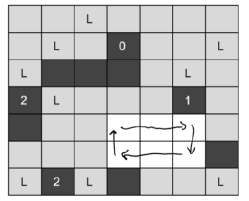
Figure 1: A Road Runner instance and a solution

3 Smarty Road Runner

Given a grid map, where each cell is either an open area (called a white cell) or a hill (called a black cell), the goal of the Smarty Road Runner game is to install laser kits on some of the white cells such that the following rules are obeyed:

• No two laser kits can shoot each other, meaning that no two laser kits can be installed in the same row or the same column, unless there is at least one black cell between them.

• A black cell may have a number that indicates the number of laser kits installed in its quadrantal neighboring cells.

• A white cell that is not covered by any laser beam is called a safe cell. All safe cells must form one closed circuit for the Road Runner to run safely, meaning that the Road Runner can start running in any safe cell, follow to an adjacent safe cell, and arrive at the starting cell, traveling all safe cells without visiting any one twice.

A laser kit, once installed, fires up horizontally and vertically, and laser beams do not stop until they reach a black cell or the edge of the grid. For example, Figure 1 shows an instance and a solution.

The following gives a Picat program for the problem.

 

import sat.

main([File]) =>
    read_data(File,MaxX,MaxY,Hill,Nums),
    Laser = new_array(MaxX,MaxY),
    Laser :: 0..1,
    Road = new_array(MaxX,MaxY),
    Road :: 0..1,
    foreach ($number(X,Y,Num) in Nums)
        sum([Laser[X1,Y1] : (X1,Y1) in [(X-1,Y), (X+1,Y), (X,Y-1), (X,Y+1)],
                            X1 >= 1, X1 =< MaxX,
                            Y1 >= 1, Y1 =< MaxY]) #= Num
    end,
    foreach (X in 1..MaxX, Y in 1..MaxY)
        (Hill[X,Y] == 1 ->
            Laser[X,Y] = 0,
            Road[X,Y] = 0
        ;
            attacked_positions(Hill,X,Y,MaxX,MaxY,Ps),
            foreach ((X1,Y1) in Ps)
                Laser[X,Y] #=> #~Laser[X1,Y1],
                Laser[X,Y] #=> #~Road[X1,Y1]
            end,
            sum([Laser[X1,Y1] : (X1,Y1) in [(X,Y)|Ps]]) #= 0 #=> Road[X,Y]
        )
    end,
    K :: 1..MaxX*MaxY,
    hcp_grid(Road,_Es,K),
    solve([$max(K)],Road),
    printf("safecircuitlen(%d).\n",K).

 

The predicate read_data reads the following items from an instance file: MaxX and MaxY are, respectively, the number of columns and the number of rows, of the grid, counting from 1; Hill is a 2-dimensional 0/1 array, where an 1 entry indicates a black cell, and a 0 entry indicates a white cell; Nums is a list of terms of the form number(X,Y,Num), which indicates that there must be Num lasers installed in (X,Y)’s neighbors.

The model uses a 2-dimensional array of Boolean variables, Laser, to indicate where lasers are installed, and another 2-dimensional array of Boolean variables, Road, to indicate the safe cells. The first foreach loop ensures that the required numbers of lasers are installed as specified in the input.

The second foreach loop in the program enforces the relationship between the Laser and Road arrays. For each cell position (X,Y), if the cell is a hill, then both Laser[X,Y] and Road[X,Y] are bound to 0, meaning that the cell can neither be a laser cell nor a road cell. Otherwise, the following actions are taken: (1) the call attacked_positions(Hill,X,Y,MaxX,MaxY,Ps) finds a list, Ps, of the positions that are under attack by laser beams originating at (X,Y); the foreach loop enforces that, if the cell at (X,Y) is a laser cell, then none of the positions in Ps can be a road or a laser cell; (3) the constraint

    sum([Laser[X1,Y1] : (X1,Y1) in [(X,Y)|Ps]]) #= 0 #=> Road[X,Y]

ensures that, if no lasers are installed in any of the attacked positions, then (X,Y) is a road cell.

The predicate attacked_positions is defined as follows:

attacked_positions(Hill,X,Y,MaxX,MaxY,Ps) =>
    Ps = [(X1,Y) : X1 in X-1..-1..1, until(Hill[X1,Y] == 1)] ++
         [(X1,Y) : X1 in X+1..MaxX, until(Hill[X1,Y] == 1)] ++
         [(X,Y1) : Y1 in Y-1..-1..1, until(Hill[X,Y1] == 1)] ++
         [(X,Y1) : Y1 in Y+1..MaxY, until(Hill[X,Y1] == 1)].

A list comprehension is utilized to collect the positions that are under attack by the laser beam in each of the four directions, and Ps is bound to the concatenation of the four lists created by the list comprehensions. Picat translates a list comprehension into a foreach loop that uses an assignment (:=) to accumulate values [26]. The until($Condition$) expression describes a terminating condition for the loop.

The hcp_grid constraint ensures that all the road cells form a cycle. It constrains K to be the total number of road cells:

    K #= sum([Road[X,Y] : X in 1..MaxX, Y in 1..MaxY])

The lower bound of K is 1, which ensures that there is at least one safe cell for the runner.

The objective of the problem is to find a subgraph such that K is maximized. The actual route is not required. If it were, it could be retrieved from the list of edges returned by hcp_grid.

4 Masyu

Masyu is a logic puzzle played on a square grid. Some of the cells are marked with black circles, some are marked with white circles, and the rest are empty. The goal of the puzzle is to draw a single loop on the board, without crossings, that passes through all the black and white circles in the following fashion:

• White circles must be passed through in a straight line, but the loop must turn in the previous and/or the next cell.

• Black circles must be turned upon, and the loop must travel straight through the next and the previous cell.

• The loop can pass through any number of empty cells, as long as there are no crossings.

Figure 2 shows an instance and its solution.

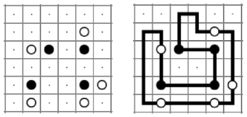
Figure 2: A Masyu instance and its solution

The following gives a Picat program for the Masyu problem.

 

import util, sat.

main([File]) =>
    read_data(File,N,Board,Grid),
    hcp_grid(Grid,Es),
    EMap = new_map(),
    foreach ({(R1,C1), (R2,C2), B} in Es)
        EMap.put({R1,C1,R2,C2}, B)
    end,
    foreach(R in 1..N, C in 1..N)
        if Board[R,C] == w then
            constrain_w(N,EMap,R,C)
        elseif Board[R,C] == b then
            constrain_b(N,EMap,R,C)
        end
    end,
    solve((Grid,values(EMap))),
    output(EMap).

 

The predicate read_data reads the following items from an instance file: N is the grid size; Board is a 2-dimensional N$\times$N array that represents the configuration of the board, where white circles are denoted by the atom w and black circles are denoted by the atom b; Grid is a 2-dimensional N$\times$N array of Boolean variables, where the entries of white and black circles are all set to be 1, indicating that the loop passes through these cells, and the entries of empty cells are free variables.

The hcp_grid(Grid,Es) constraint ensures that all the cells that are labeled 1 in Grid form a loop represented by a list of directed edges Es. A directed edge in Es has the form {(R1,C1),(R2,C2),B}, where (R1,C1) and (R2,C2) are two cell positions, and B is a Boolean variable that is equal to 1 if and only if the edge from (R1,C1) to (R2,C2) is included in the loop.

The loop must obey the rules when passing through black and white circles. In order to facilitate the use of Es returned by hcp_grid, the implementation converts Es to a map. A triplet {(R1,C1),(R2,C2),B} is converted to a key-value pair, where the key is {R1,C1,R2,C2} and the value is B. The map makes it possible to retrieve the edge variable of a given edge in constant time.

The predicate constrain_w(N,EMap,R,C), which is defined below, constrains how the loop passes through the white cell at (R,C).

constrain_w(N,EMap,R,C) =>
    Ps = [[(R,C-1), (R,C), (R,C+1), (R-1,C+1)],
          [(R,C-1), (R,C), (R,C+1), (R+1,C+1)],
          [(R-1,C-1), (R,C-1), (R,C), (R,C+1)],
          [(R+1,C-1), (R,C-1), (R,C), (R,C+1)],
          [(R-1,C-1), (R-1,C), (R,C), (R+1,C)],
          [(R-1,C+1), (R-1,C), (R,C), (R+1,C)],
          [(R-1,C), (R,C), (R+1,C), (R+1,C-1)],
          [(R-1,C), (R,C), (R+1,C), (R+1,C+1)]],
    constrain_paths(N,EMap,Ps).

There must be a line in the loop that passes through the cell horizontally or vertically, and the loop must turn in the previous and/or the next cell. The predicate collects 8 path shapes into the variable Ps. Each path shape represents 2 paths, with the path shape itself representing one path and its reverse representing the other one. So, there are, in total, 16 possible ways that the loop passes through the white cell. For example, the path

(R,C-1) $\rightarrow$ (R,C) $\rightarrow$ (R,C+1) $\rightarrow$ (R-1,C+1)

enters (R,C) from left, moves on to right, and turns up at (R,C+1).

Let B1 be the edge variable of (R,C-1) $\rightarrow$ (R,C), B2 be the edge variable of (R,C) $\rightarrow$ (R,C+1), and B3 be the edge variable of (R,C+1) $\rightarrow$ (R-1,C+1). The above path is included in the loop if B1 #/\ B2 #/\ B3 is satisfied.

Some of the path shapes in Ps may not be valid because they contain coordinates that fall outside of the grid. The predicate constrain_paths(N,EMap,Ps) generates constraints to ensure that at least one of the valid path shapes in Ps occurs in the loop.

The predicate constrain_b(N,EMap,R,C) constrains how the loop passes through the black cell at (R,C). The loop must make a turn at (R,C), and must travel straight through the next and the previous cell. In total, there are 8 possible ways that the loop passes through the black cell, among which the following is one:

(R,C-2) $\rightarrow$ (R,C-1) $\rightarrow$ (R,C) $\rightarrow$ (R+1,C) $\rightarrow$ (R+2,C)

The path enters (R,C) horizontally from left, and turns down at (R,C).

The predicate solve((Grid,values(EMap))) retrieves the vertex variables from Grid and the edge variables from EMap, and labels these variables such that the constraints are satisfied.

5 Shingoki

Shingoki is a logic puzzle, similar to Masyu, played on a square grid. Some of the cells are marked with black circles, some are marked with white circles, and the rest are empty. The goal of the puzzle is to draw a single loop, without crossings, that passes through all the black and white circles. White circles must be passed through in a straight line, and black circles must be turned upon. In Shingoki, each marked cell also has a number on it, which constrains the length of the two lines connected at the cell.

Figure 3 shows an instance of Shingoki and its solution. The cell marked with 4 is a black circle. The loop turns on the circle. The horizontal line connecting to it has length 3, and the vertical line connecting to it has length 1, making the total length equal to 4.

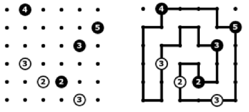
Figure 3: A Shingoki instance and its solution

The following shows a Picat program for Shingoki.

 

main([File]) =>
    read_data(File,N,Board,Grid),
    hcp_grid(Grid,Es),
    EMap = new_map(),
    foreach ({(R1,C1), (R2,C2), B} in Es)
        EMap.put({R1,C1,R2,C2}, B)
    end,
    foreach(R in 1..N, C in 1..N)
        if Board[R,C] = $w(Clue) then
            constrain_w(N,EMap,R,C,Clue)
        elseif Board[R,C] = $b(Clue) then
            constrain_b(N,EMap,R,C,Clue)
        end
    end,
    solve((Grid,values(EMap))),
    output(EMap).

 

The read_data predicate is the same as the one in the Masyu program, except that Board is a 2-dimensional N$\times$N array that represents the configuration of the board, where an entry w(Clue) indicates a white circle with a clue number, and an entry b(Clue) indicates a black circle with a clue number.

The predicate constrain_w(N,EMap,R,C,Clue), which is defined below, constrains how the loop passes through the white cell at (R,C), which has the clue number Clue.

constrain_w(N,EMap,R,C,Clue) =>
    Ps = [],
    foreach (D1 in 1..Clue-1, D2 = Clue-D1)
        V = [(R1,C) : R1 in R-D1..R+D2],
        P1 = [(R-D1,C-1)] ++ V ++ [(R+D2,C-1)],
        P2 = [(R-D1,C-1)] ++ V ++ [(R+D2,C+1)],
        P3 = [(R-D1,C+1)] ++ V ++ [(R+D2,C-1)],
        P4 = [(R-D1,C+1)] ++ V ++ [(R+D2,C+1)],
        H = [(R,C1) : C1 in C-D1..C+D2],
        P5 = [(R-1,C-D1)] ++ H ++ [(R-1,C+D2)],
        P6 = [(R-1,C-D1)] ++ H ++ [(R+1,C+D2)],
        P7 = [(R+1,C-D1)] ++ H ++ [(R-1,C+D2)],
        P8 = [(R+1,C-D1)] ++ H ++ [(R+1,C+D2)],
        Ps := [P1,P2,P3,P4,P5,P6,P7,P8|Ps]
    end,
    constrain_paths(N,EMap,Ps).

There must be a line of length Clue passing through the cell, and the line can be split into two segments. The foreach loop considers all possible splits, with D1 being the length of the first segment and D2 being the length of the second segment (D1+D2 = Clue). The line can be either vertical or horizontal. The variable V refers to a list of cell positions in the vertical line, and the variable H refers to a list of cell positions in the horizontal line. Depending on how the loop turns at the ends of the line segments, there are, in total, 8 possible shapes of paths going through the cell. Each path shape represents two paths. So, there are, in total, 16 possible paths. The predicate collects all the path shapes into a variable Ps using assignments, and calls constrain_paths(N,EMap,Ps) to ensure that at least one of the path shapes in Ps occurs in the loop.

The predicate constrain_b(N,EMap,R,C,Clue) is defined similarly. As the loop turns on a black circle, two line segments connect orthogonally at the cell, and there are 4 possible connections, namely, $\lceil$, $\rceil$, $\lfloor$, and $\rfloor$. Counting in the possible ways the loop turns at the ends of the line segments, there are up to 16 possible shapes of paths going through a black cell.

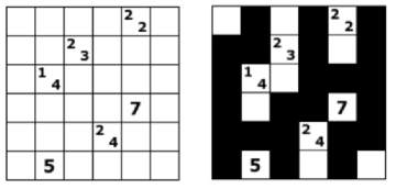
Figure 4: A Tapa instance and its solution

6 Tapa

Tapa is another logic puzzle played on a square grid. Initially, some of the cells are filled with clue numbers and all others are empty. The goal of the puzzle is to color each of the cells black or white such that the following constraints are satisfied:

• The black cells form a single polyomino, connected orthogonally in a single group.

• There are no 2$\times$2 black areas.

• The clue numbers are respected.

A clue number indicates the size of a connected block of black cells in the surrounding neighbors, including diagonally connected neighbors. A cell can be filled with up to 4 clue numbers. If there are 2 or more clue numbers in a cell, then there must be at least 1 white cell between each 2 black blocks. The blocks can appear in any order. Figure 4 gives a Tapa instance and its solution. It can be checked that the solution respects all the clue numbers. For example, for the clue numbers 1 and 4 on the cell (3,2), row 3 and column 2, there is a block of size 1 at (4,3) and a block of size 4 occupying (2,1), (2,2), (3,1), and (4,1).

The following gives a Picat program for the Tapa problem.

 

main([File]) =>
    read_data(File,N,Board,Grid),
    scc_grid(Grid),
    foreach (R in 1..N-1, C in 1..N-1)
        Grid[R,C] + Grid[R,C+1] + Grid[R+1,C] + Grid[R+1,C+1] #< 4
    end,
    foreach (R in 1..N, C in 1..N, nonvar(Board[R,C]))
        neibs(N,R,C,NeibArr),
        constrain_blocks(Board[R,C],Grid,NeibArr)
    end,
    solve(Grid),
    output(Grid).

neibs(N,R,C,NeibArr) =>
    NeibArr = {(R1,C1) :  (R1,C1) in [(R-1,C-1), (R-1,C), (R-1,C+1), (R,C+1),
                                      (R+1,C+1), (R+1,C), (R+1,C-1), (R,C-1)],
                           R1 >= 1, R1 =< N, C1 >= 1, C1 =< N}.

 

The predicate read_data reads the following items from an instance file: N is the grid size; Board is a 2-dimensional N$\times$N array that represents the configuration of the board, where a non-variable entry indicates a list of clue numbers; Grid is a 2-dimensional N$\times$N array of Boolean variables, where a variable is labeled 1 if the cell is colored black, and 0 otherwise.

The scc_grid(Grid) constraint ensures that all the black cells form a strongly connected component. The first foreach loop ensures there are no 2$\times$2 black areas. The second foreach loop ensures that the clue numbers are respected. For each entry (R,C), if there are clue numbers filled in the cell, meaning that nonvar(Board[R,C]) is true, then the program ensures the existence of the given clue numbers of blocks in the neighbors.

The call neibs(N,R,C,NeibArr) binds NeibArr to an array of neighboring positions surrounding (R,C). An array is more convenient than a list because the positions are circular.

The predicate constrain_blocks is defined as follows:

constrain_blocks(Clues,Grid,NeibArr) =>
    findall_layouts(Clues,NeibArr,Layouts),
    Bs = [],
    foreach (Layout in Layouts)
        B :: 0..1,
        LayoutBs = [cond(Layout[I] == 1, Grid[R,C], #~Grid[R,C]) :
                        I in 1..len(NeibArr), NeibArr[I] = (R,C)],
        B #= min(LayoutBs),
        Bs := [B|Bs]
    end,
    sum(Bs) #>= 1.

The predicate findall_layouts(Clues,NeibArr,Layouts) finds all the possible layouts of the blocks of the given sizes as indicated by Clues. A layout is an array where, an entry is 0 if the corresponding neighbor cell is free, and 1 if the corresponding neighbor cell is occupied by a block. For example, the cell at (3,2), row 3 and column 2, in Figure 4 has the following array of neighbors:

    NeibArr = {(2,1), (2,2), (2,3), (3,3), (4,3), (4,2), (4,1), (3,1)}

The layout of the two blocks, of size 1 and size 4, respectively, given in Figure 4 is represented by the following layout:

    {1, 1, 0, 0, 1, 0, 1, 1}

The conditional expression cond(Layout[I] == 1, Grid[R,C], #~Grid[R,C]) is equal to Grid[R,C] if Layout[I] == 1, and #~Grid[R,C] otherwise. For each layout, a Boolean variable B is utilized to indicate if the blocks have the layout. The constraint sum(Bs) #>= 1 ensures that the blocks have at least one of the layouts.

7 Implementation and Experimental Results

Several SAT encodings are available for the HCP problem [11, 19, 23, 15, 25, 12]. If a graph has more than one vertex, then each vertex must have exactly one incoming edge and exactly one outgoing edge, and all the edges must form exactly one cycle. The degree constraints can be encoded easily. The focus of the encodings for HCP has been on how to ensure the reachability of all the in-vertices and ban sub-cycles. A common technique used is to impose a strict ordering on the vertices. The distance encoding chooses a vertex to serve as the starting vertex, and assigns a distinct distance to each of the in-vertices. If there is an edge from $v_{\_}i$ to $v_{\_}j$, then $v_{\_}j$’s distance is the successor of $v_{\_}i$’s, unless $v_{\_}j$ is the starting vertex. The successor function can be encoded in several different ways. In the implementation in Picat, the binary adder encoding is used, which has been found to be the most effective [25].

In contrast to HCP, no studies have been reported on encoding SCC into SAT. The challenge is centered on how to enforce the reachability of all the in-vertices. The satisfiability modulo acyclicity approach [4] avoids encoding the constraint by performing reachability checking at solving time. The Picat implementation of scc employs an encoding, named tree encoding, which utilizes the property that every strongly connected graph has at least one spanning tree. The tree encoding chooses a vertex as the root of a tree, chooses a parent for each non-root vertex, and assigns a distance to each vertex, with 0 being assigned to the root, and the distance assigned to each non-root vertex being 1 greater than that assigned to its parent.

For optimization problems, Picat uses branch-and-bound to optimize the objective. It first posts the problem as a constraint satisfaction problem, ignoring the objective. Once a solution is found, Picat uses binary search to find a solution with the optimum value. Each time the lower or upper bound is updated, Picat starts the SAT solver from scratch.

The rest of this section gives the execution times of the programs run using Picat version 3.1 on a Windows machine (Intel i7 3.30GHz CPU and 64G RAM). Picat provides C interfaces to several SAT solvers, with Maple as the default. The execution times reported below were obtained using Maple and Kissat version 1.0.3.

For the sake of comparison, the execution times of the ASP programs for the problems provided by the LP/CP competition organizers run with Clingo version 5.5.0 are also included. The reachability constraint is encoded neatly in ASP as follows:

    reach(V) :- start(V).
    reach(V) :- reach(U), edge(U,V).
    :- in(V), not reach(V).

It ensures that there is a path from the starting vertex to every in-vertex. Clingo adopts the lazy approach to reachability checking [4].

Table 1 shows the execution times, which include both translation and solving times. The column Benchmark gives the instances, where the graph sizes are shown in parentheses. Picat(Kissat) is a clear winner. While Picat(Kissat) and Clingo demonstrate similar performance on Roadrunner and Tapa, Picat(Kissat) is more than 10 times as fast as Clingo on Masyu and Shingoki.

Table 1: Execution times (seconds)

Benchmark	Picat(Kissat)	Picat(Maple)	Clingo
Roadrunner6 (20$\times$20)	0.82	1.84	0.54
Roadrunner7 (20$\times$20)	5.05	42.52	1.33
Roadrunner8 (30$\times$30)	6.99	55.70	10.75
Masyu3 (30$\times$30)	1.62	6.94	22.37
Masyu4 (35$\times$35)	3.95	9.03	48.84
Masyu5 (40$\times$40)	6.21	11.72	96.78
Shingoki3 (31$\times$31)	2.89	7.11	27.28
Shingoki4 (36$\times$36)	5.26	8.59	57.42
Shingoki5 (41$\times$41)	8.62	14.23	111.62
Tapa3 (25$\times$25)	0.43	1.40	0.61
Tapa4 (30$\times$30)	0.62	3.74	0.97
Tapa5 (35$\times$35)	0.99	5.29	1.72

8 Conclusion

This paper presents the newly added graph constraints in Picat, and their use in modeling and solving four graph synthesis problems selected from the recent LP/CP competitions. The programs demonstrate the modeling capabilities of the Picat language. Picat provides several language constructs that are not present in standard Prolog, including functions, arrays, loops, list/array comprehensions, and assignments. With the graph constraints and these language constructs, Picat can serve as a powerful modeling language for various constraint solvers. The Picat programs compare favorably well in terms of conciseness with the ASP programs. As a general-purpose language, Picat has the advantage over many other modeling languages in handling I/O and integration with other software components.

The Picat programs also demonstrate the solving efficiency of the cutting-edge SAT solvers empowered with effective encodings. The bottleneck in solving the problems is ensuring the reachability of all the in-vertices. When the hcp and scc constraints are removed from the programs, all of the problem instances become trivial and can be solved in a flash. Picat follows the eager approach, first encoding constraints into SAT and then using a SAT solver to solve the encoding. This paper has shown that the eager approach is competitive with the lazy approach used in Clingo. With the advancement of SAT solvers and inventions of novel encoding methods, the eager approach will become ever more appealing.

The encodings for the hcp and scc constraints are the results of an extensive comparison study. Nevertheless, they are not meant to be optimal, and further research is warranted to find even better encodings. For optimization problems, such as the Road Runner problem, using an incremental SAT solver could lead to better performance. Furthermore, it is worthwhile to investigate translation of the graph constraints to SMT that supports checking of graph reachability at solving time.

References

- [1]
- [2] Nicolas Beldiceanu, Mats Carlsson & Jean-Xavier Rampon (2021): Global Constraint Catalog. http://sofdem.github.io/gccat/gccat/.
- [3] Armin Biere, Marijn Heule, Hans van Maaren & Toby Walsh, editors (2009): Handbook of Satisfiability. Frontiers in Artificial Intelligence and Applications 185, IOS Press.
- [4] Jori Bomanson, Martin Gebser, Tomi Janhunen, Benjamin Kaufmann & Torsten Schaub (2016): Answer Set Programming Modulo Acyclicity. Fundam. Informaticae 147(1), pp. 63–91, 10.3233/FI-2016-1398.
- [5] Lucas Bordeaux, Youssef Hamadi & Lintao Zhang (2006): Propositional Satisfiability and Constraint Programming: A comparative survey. ACM Comput. Surv. 38(4), pp. 1–54. Available at http://doi.acm.org/10.1145/1177352.1177354.
- [6] Gerhard Brewka, Thomas Eiter & Miroslaw Truszczyński (2011): Answer Set Programming at a Glance. Commun. ACM 54(12), pp. 92–103. 10.1017/S1471068407003250
- [7] Mehmet Dincbas, Pascal Van Hentenryck, Helmut Simonis, Abderrahmane Aggoun, Thomas Graf & Françoise Berthier (1988): The Constraint Logic Programming Language CHIP. In: FGCS, pp. 693–702.
- [8] Sergii Dymchenko & Mariia Mykhailova (2015): Declaratively Solving Google Code Jam Problems with Picat. In: PADL, pp. 50–57, 10.1007/978-3-319-19686-2_4.
- [9] Robert Fourer & David M. Gay (2002): Extending an Algebraic Modeling Language to Support Constraint Programming. INFORMS J. Comput. 14(4), pp. 322–344, 10.1287/ijoc.14.4.322.2825.
- [10] Pascal Van Hentenryck (2002): Constraint and Integer Programming in OPL. INFORMS J. Comput. 14(4), pp. 345–372, 10.1287/ijoc.14.4.345.2826.
- [11] Alexander Hertel, Philipp Hertel & Alasdair Urquhart (2007): Formalizing Dangerous SAT Encodings. In: SAT, 4501, pp. 159–172, 10.1007/978-3-540-72788-0_18.
- [12] Marijn J. H. Heule (2021): Chinese Remainder Encoding for Hamiltonian Cycles. In: SAT, pp. 216–224, 10.1007/978-3-030-80223-3_15.
- [13] Jinbo Huang (2008): Universal Booleanization of Constraint Models. In: CP, pp. 144–158, 10.1007/978-3-540-85958-1_10.
- [14] Peter Jeavons & Justyna Petke (2012): Local Consistency and SAT-Solvers. J. Artif. Intell. Res. 43, pp. 329–351, 10.1613/jair.3531.
- [15] Andrew Johnson (2014): Quasi-linear reduction of Hamiltonian cycle problem (HCP) to satisfiability problem (SAT). Available at https://priorart.ip.com/IPCOM/000237123.
- [16] Donald Knuth (2015): The Art of Computer Programming, Volume 4, Fascicle 6: Satisfiability. Addison-Wesley.
- [17] Sharad Malik & Lintao Zhang (2009): Boolean satisfiability from theoretical hardness to practical success. Commun. ACM 52(8), pp. 76–82, 10.1145/1536616.1536637.
- [18] Nicholas Nethercote, Peter J. Stuckey, Ralph Becket, Sebastian Brand, Gregory J. Duck & Guido Tack (2007): MiniZinc: Towards a Standard CP Modelling Language. In: CP, pp. 529–543, 10.1007/978-3-540-74970-7_38.
- [19] Steven David Prestwich (2003): SAT problems with chains of dependent variables. Discret. Appl. Math. 130(2), pp. 329–350, 10.1016/S0166-218X(02)00410-9.
- [20] Mirko Stojadinovic & Filip Maric (2014): meSAT: multiple encodings of CSP to SAT. Constraints An Int. J. 19(4), pp. 380–403, 10.1007/s10601-014-9165-7.
- [21] Peter J. Stuckey, Kim Marriott & Guido Tack (2021): The MiniZinc Handbook. https://www.minizinc.org/doc-2.5.5/en/index.html.
- [22] Naoyuki Tamura, Akiko Taga, Satoshi Kitagawa & Mutsunori Banbara (2009): Compiling finite linear CSP into SAT. Constraints An Int. J. 14(2), pp. 254–272, 10.1007/s10601-008-9061-0.
- [23] Miroslav N. Velev & Ping Gao (2009): Efficient SAT Techniques for Absolute Encoding of Permutation Problems: Application to Hamiltonian Cycles. In: SARA, AAAI. Available at http://www.aaai.org/ocs/index.php/SARA/SARA09/paper/view/837.
- [24] Toby Walsh (2000): SAT v CSP. In: CP, pp. 441–456, 10.1007/3-540-45349-0_32.
- [25] Neng-Fa Zhou (2020): In Pursuit of an Efficient SAT Encoding for the Hamiltonian Cycle Problem. In: CP, pp. 585–602, 10.1007/978-3-030-58475-7_34.
- [26] Neng-Fa Zhou & Jonathan Fruhman (2017): Canonicalizing High-Level Constructs in Picat. In: PADL, pp. 19–33, 10.1007/978-3-319-51676-9_2.
- [27] Neng-Fa Zhou & Håkan Kjellerstrand (2017): Optimizing SAT Encodings for Arithmetic Constraints. In: CP, pp. 671–686, 10.1007/978-3-319-66158-2_43.
- [28] Neng-Fa Zhou, Håkan Kjellerstrand & Jonathan Fruhman (2015): Constraint Solving and Planning with Picat. Springer Briefs in Intelligent Systems, Springer, 10.1007/978-3-319-25883-6.