Hard to Forget: Poisoning Attacks on Certified Machine Unlearning

Abstract

The right to erasure requires removal of a user’s information from data held by organizations, with rigorous interpretations extending to downstream products such as learned models. Retraining from scratch with the particular user’s data omitted fully removes its influence on the resulting model, but comes with a high computational cost. Machine “unlearning” mitigates the cost incurred by full retraining: instead, models are updated incrementally, possibly only requiring retraining when approximation errors accumulate. Rapid progress has been made towards privacy guarantees on the indistinguishability of unlearned and retrained models, but current formalisms do not place practical bounds on computation. In this paper we demonstrate how an attacker can exploit this oversight, highlighting a novel attack surface introduced by machine unlearning. We consider an attacker aiming to increase the computational cost of data removal. We derive and empirically investigate a poisoning attack on certified machine unlearning where strategically designed training data triggers complete retraining when removed.

Keywords machine unlearning  $\cdot$ adversarial machine learning  $\cdot$ data poisoning

1 Introduction

Much of modern machine learning has been advanced by the availability of large volumes of data. However, organizations that collect user data must comply with data protection regulations and often prioritize privacy to mitigate risk of civil litigation and reputational damage. Prominent regulations—i.e., GDPR [16] and CCPA [10]—encode a right to erasure—organizations must “erase personal data without undue delay” when requested. When tested, such regulations have been found to extend to products derived from personal data, including trained models [21]. [54] argue that models could be legally classified as personal data, which agrees with the draft guidance from the [53] that “erasure of the data… may not be possible without retraining the model… or deleting the model altogether”. Such concerns are justified by a legitimate privacy risk: training data can be practically reconstructed from models [20, 49, 54].

Naïvely erasing data from a model by full retraining can be computationally costly. This has motivated the recent study of machine unlearning: how to efficiently undo the impact of data on a model. [26] develop an approximate update which is 3 orders of magnitude faster than retraining, or supporting up to 10,000 approximate updates before retraining is required, with only a small drop in accuracy. [22] find a $100\times$ improvement in deletion efficiency with comparable clustering quality. Theoretical investigations has led to guarantees on privacy (indistinguishability of unlearned models with retrained models), but have largely ignored computation cost.

In an adversarial setting where risks to privacy motivate unlearning, we advocate that computation should also be viewed under an adversarial lens. While the aforementioned empirical results paint an optimistic picture for machine unlearning, such work assumes passive users who are trusted: they work within provided APIs, but also don’t attempt to harm system performance in any way. In this paper we consider an active adversary as is more typical in the adversarial learning field [31]. Users in this work can issue strategically chosen data for learning, and then request their data be unlearned. We adopt a typical threat model where users may apply a bounded perturbation to their (natural) data. Boundedness is motivated by a desire to remain undetected. Under this threat model we identify a new vulnerability: poisoning attacks that effectively slow down unlearning.

We highlight several perspectives on our results. They call into question the extent to which unlearning improves performance over full retraining which achieves complete indistinguishability. Our work highlights the risk of deploying approximate unlearning algorithms with data-dependent running times. And more broadly we show that data poisoning can harm computation beyond only accuracy—analogous to conventional denial-of-service attacks.

Contributions.

We identify a new vulnerability of machine learning systems. Our suite of experiments considers: the attack’s effect in a wide range of parameter settings; both white-box and grey-box attacks; a range of perturbation geometries and bounds; trade-offs between optimality of the attacker’s objective and time to compute the attack; and the feasibility of running the attack long term.

2 Preliminaries

This section sets the scene for our attack. We introduce the target of our attack in Sec. 2.1—learning systems that support data erasure requests via machine unlearning. We then review a certified machine unlearning method that we use to demonstrate our attack. Sec. 2.3 closes with a discussion of the vulnerability and our assumed threat model. Table 1 summarizes notation used throughout the paper.

2.1 Machine learning on user data

Consider an organization that trains machine learning models using data from consenting users. In line with privacy regulations, the organization allows users to revoke consent at any time and submit an erasure request for some (or all) of their data. When fulfilling an erasure request, the organization takes a cautious approach to user privacy—erasing the user’s raw data and removing the data’s influence on trained models. We assume erasing raw data (e.g. from a database) is straightforward and focus here on the task of removing data from a trained model.

Formally, let $\mathcal{Z}^{\ast}$ be the space of training datasets consisting of samples from an example space $\mathcal{Z}$. Given a training dataset $D\in\mathcal{Z}^{\ast}$, the organization deploys a learning algorithm that returns a model $A(D)$ in hypothesis space $\mathcal{H}$. To support erasure requests, the organization also deploys an unlearning algorithm $M$ which, given a training dataset $D\in\mathcal{Z}^{\ast}$, a subset $D^{\prime}\subset D$ to erase and a model $h\sim A(D)$, returns a sanitized model $M(D,D^{\prime},h)\in\mathcal{H}$ that is approximately (to be made mathematically precise below) $A(D\setminus D^{\prime})$. We allow $A$ and $M$ to be randomized algorithms—each can be interpreted as specifying a distribution over $\mathcal{H}$ conditioned on their inputs.

To ensure no trace of the erased data is left behind, we assume $A$ and $M$ satisfy a rigorous definition of unlearning. Specifically, we assume the distribution of unlearned models $M(D,D^{\prime},A(D))$ is statistically indistinguishable from the distribution of models retrained on the remaining data $A(D\setminus D^{\prime})$. This is known as approximate unlearning and there are variations depending on how statistical indistinguishability is defined. For concreteness, we adopt the unlearning definition and algorithms of [26], which we review in the next section.

Table 1: Summary of notation.

Notation	Explanation
$A$	Learning algorithm
$M$	Unlearning algorithm
$D$, $D_{\mathrm{psn}}$, $D_{\mathrm{cln}}$	Dataset (generic, poisoned, clean)
$\bm{\mathrm{X}}$, $\bm{\mathrm{X}}_{\mathrm{psn}}$, $\bm{\mathrm{X}}_{\mathrm{cln}}$	Feature matrix (generic, poisoned, clean)
$\mathcal{H}$	Hypothesis space for model
$\bm{\mathrm{\theta}}$	Model parameters
$R$, $R_{\bm{\mathrm{b}}}$	Learning objective (unperturbed, perturbed)
$\bm{\mathrm{b}}$	Objective perturbation coefficients
$\sigma$	Standard deviation of $\bm{\mathrm{b}}$
$\lambda$	Regularization strength
$\ell$	Loss function
$\gamma$	Lipschitz constant of $\ell^{\prime\prime}$
$\epsilon,\delta$	Indistinguishability parameters
$\beta$	Bound on gradient norm of $R_{\bm{\mathrm{b}}}$
$C$	Attacker’s estimate of unlearning cost
$\{g_{j}\}$	Attacker’s inequality constraints

2.2 Certified removal

This section reviews learning/unlearning algorithms for linear models proposed by [26]. The algorithms satisfy a definition of approximate unlearning called certified removal, where indistinguishability is defined in a similar manner as $(\epsilon,\delta)$-differential privacy [19].

Definition 1.

Given $\epsilon,\delta>0$ a removal mechanism $M$ performs $(\epsilon,\delta)$-certified removal for learning algorithm $A$ if $\forall\mathcal{T}\subseteq\mathcal{H},D\in\mathcal{Z}^{\ast},\bm{\mathrm{z}}\in D$:

$$P(M(D,\{\bm{\mathrm{z}}\},A(D))\in\mathcal{T})\leq e^{\epsilon}P(A(D\setminus\{\bm{\mathrm{z}}\})\in\mathcal{T})+\delta$$

and

$$P(A(D\setminus\{\bm{\mathrm{z}}\})\in\mathcal{T})\leq e^{\epsilon}P(M(D,\{\bm{\mathrm{z}}\},A(D))\in\mathcal{T})+\delta.$$

The learning/unlearning algorithms we consider support linear models that minimize a regularized empirical risk of the form:

$$R(\bm{\mathrm{\theta}};D)=\sum_{(\bm{\mathrm{x}},y)\in D}\left\{\ell(\bm{\mathrm{\theta}}^{\top}\bm{\mathrm{x}},y)+\frac{\lambda}{2}\|\bm{\mathrm{\theta}}\|_{2}^{2}\right\}$$ (1)

where $\bm{\mathrm{\theta}}\in\mathbb{R}^{d}$ is a vector of learned weights, $\ell:\mathbb{R}\times\mathbb{R}\to\mathbb{R}$ is a convex loss that is differentiable everywhere, and $\lambda>0$ is a regularization hyperparameter. Note that we are assuming the instance space $\mathcal{Z}$ is the product of a feature space $\mathcal{X}\subseteq\mathbb{R}^{d}$ and a label space $\mathcal{Y}\subseteq\mathbb{R}$. Thus supervised regression and classification are supported.

Learning algorithm.

Since unlearning is inexact (see below), random noise is injected during learning to ensure indistinguishability. Concretely, the original minimization objective $R(\bm{\mathrm{\theta}};D)$ is replaced by a perturbed objective

$$R_{\bm{\mathrm{b}}}(\bm{\mathrm{\theta}};D)=R(\bm{\mathrm{\theta}};D)+\bm{\mathrm{b}}^{\top}\bm{\mathrm{\theta}},$$ (2)

where $\bm{\mathrm{b}}\in\mathbb{R}^{d}$ is a vector of coefficients drawn i.i.d. from a standard normal distribution with standard deviation $\sigma$. The resulting perturbed learning problem can be solved using standard convex optimization methods. This procedure is summarized in pseudocode below.

1:procedure $A$($D$)

2:     $\bm{\mathrm{b}}\sim\operatorname{Normal}(\bm{\mathrm{0}},\sigma\cdot\mathbb{I}_{d})$

3:     $\bm{\mathrm{\theta}}^{\star}\leftarrow\arg\min_{\bm{\mathrm{\theta}}}R_{\bm{\mathrm{b}}}(\bm{\mathrm{\theta}};D)$

4:     $\beta\leftarrow 0$ $\triangleright$ initial gradient residual norm is zero

5:     return $\bm{\mathrm{\theta}}^{\star},\beta$

6:end procedure

Algorithm 1 Learning algorithm for certified removal

Unlearning algorithm.

Approximate unlearning is done by perturbing the model parameters $\bm{\mathrm{\theta}}$ towards the optimizer of the new objective $R_{\bm{\mathrm{b}}}(\bm{\mathrm{\theta}};D\setminus D^{\prime})$. The perturbation is computed as

$$\Delta\bm{\mathrm{\theta}}=-\mathcal{I}(D^{\prime};D,\bm{\mathrm{\theta}})$$

where $D$ is the initial training data, $D^{\prime}\subset D$ is the data to erase, $\bm{\mathrm{\theta}}$ are the initial model parameters and

$$\mathcal{I}(D^{\prime};D,\bm{\mathrm{\theta}})=-\left[\mathrm{H}_{\bm{\mathrm{\theta}}}R_{\bm{\mathrm{b}}}(\bm{\mathrm{\theta}};D)\right]^{-1}\nabla_{\bm{\mathrm{\theta}}}R(\bm{\mathrm{\theta}};D^{\prime})$$ (3)

is the influence function [15, 33]. The influence function approximates the change in $\bm{\mathrm{\theta}}$ when $D$ is augmented by $D^{\prime}$. The first factor in (3) is the inverse Hessian of the objective evaluated on $D$ and the second factor is the gradient of the objective evaluated on $D^{\prime}$.

Since the update $\bm{\mathrm{\theta}}\leftarrow\bm{\mathrm{\theta}}+\Delta\bm{\mathrm{\theta}}$ is approximate, it is not guaranteed to minimize the new objective exactly. This becomes a problem for indistinguishability if the error in $\bm{\mathrm{\theta}}$ is so large that it is not masked by the noise added during learning. To ensure indistinguishability, the unlearning algorithm maintains an upper bound on the gradient residual norm (GRN) $\|\nabla R_{\bm{\mathrm{b}}}(\bm{\mathrm{\theta}}+\Delta\bm{\mathrm{\theta}};D\setminus D^{\prime})\|_{2}$ and resorts to retraining from scratch if a trigger value is exceeded. Given an initial upper bound on the GRN of $\beta$ (before $D^{\prime}$ is removed and $\bm{\mathrm{\theta}}$ is updated), the upper bound is updated as

$$\beta\leftarrow\beta+\gamma\|\mathbf{X}\|_{2}\|\Delta\bm{\mathrm{\theta}}\|_{2}\|\mathbf{X}\Delta\bm{\mathrm{\theta}}\|_{2}$$ (4)

where $\gamma$ is the Lipschitz constant of $\ell^{\prime\prime}$, $\mathbf{X}$ is the feature matrix associated with $D\setminus D^{\prime}$ and the feature vectors are assumed to satisfy $\|\bm{\mathrm{x}}\|_{2}\leq 1$ for all $(\bm{\mathrm{x}},y)\in D$. Whenever $\beta$ exceeds the trigger value

$$\beta_{\mathrm{trigger}}=\sigma\epsilon/\sqrt{2\log 3/2\delta}$$ (5)

the algorithm resorts to retraining from scratch to ensure certified removal, as proved by [26].

The entire procedure is summarized in pseudocode below.

1:procedure $M$($D,D^{\prime},h$)

2:     $\bm{\mathrm{\theta}},\beta\leftarrow h$

3:     $\Delta\bm{\mathrm{\theta}}\leftarrow-\mathcal{I}(D^{\prime};D,\bm{\mathrm{\theta}})$

4:     $D\leftarrow D\setminus D^{\prime}$

5:     $\mathbf{X}\leftarrow$ feature matrix of $D$

6:     $\beta\leftarrow\beta+\gamma\|\mathbf{X}\|_{2}\|\Delta\bm{\mathrm{\theta}}\|_{2}\|\mathbf{X}\Delta\bm{\mathrm{\theta}}\|_{2}$

7:     if $\beta>\beta_{\mathrm{trigger}}$ then

8:         $\bm{\mathrm{\theta}},\beta\leftarrow A(D)$ $\triangleright$ Retrain from scratch (slow)

9:     else

10:         $\bm{\mathrm{\theta}}\leftarrow\bm{\mathrm{\theta}}+\Delta\bm{\mathrm{\theta}}$ $\triangleright$ Approximate update (fast)

11:     end if

12:     return $\bm{\mathrm{\theta}},\beta$

13:end procedure

Algorithm 2 Unlearning algorithm for certified removal

2.3 Vulnerability and threat model

One critique of the unlearning algorithm introduced in the previous section is that it does not guarantee a reduction in computation cost compared to full retraining. In the worst case, the error of the approximate unlearning update exceeds the allowed threshold ($\beta>\beta_{\mathrm{trigger}}$) and the algorithm resorts to full retraining (line 8 in Alg. 2). We exploit this vulnerability in this paper to design an attack that triggers retraining more frequently, thereby diminishing (or even nullifying) the promised efficiency gains of unlearning.

Capabilities of the attacker.

We assume the attacker controls one or more users, who are able to modify (within limits) their training data and initiate erasure requests. In practical settings, the attacker could increase the number of users under their control by creating fake user accounts. Following standard threat models in the data poisoning literature [6, 39, 46, 48, 32] we consider attackers with white-box and grey-box access. In our white-box setting, the attacker can access training data of benign users, the architecture of the deployed model and the model state (excluding the coefficients $\bm{\mathrm{b}}$ of the random perturbation term). While this is a perhaps overly pessimistic view, it allows for a worst-case evaluation of the attack. In our grey-box setting, the attacker still has knowledge of the model architecture, but can no longer access training data of benign users nor the model state. In place of real training data, the grey-box attacker acquires surrogate data from the same or a similar distribution.

Capabilities of the defender.

For the majority of this paper, we assume the organization (the defender) is unaware that unlearning is vulnerable to slow-down attacks and does not mount any specific defenses. However, we do assume the organization conducts basic data validity checks (e.g. ensuring image pixel values are within valid ranges) and occasional manual auditing of data. To evade detection during manual auditing, we assume the attacker makes (small) bounded modifications to clean data which are unlikely to arouse suspicion.

3 Slow-down Attack

In this section, we present an attack on unlearning algorithms with data-dependent running times. We begin by formulating our attack as a generalized data poisoning problem in Sec. 3.1. Then in Sec. 3.2, we describe a practical solution based on projected gradient descent under some simplifying assumptions. Finally, in Sec. 3.3 we propose concrete objectives for the attacker and suggest further relaxations to speed-up the attack.

3.1 Formulation as a data poisoning problem

Let $D$ be data used by the organization (the defender) to train (with learning algorithm $A$) an initial model $\hat{h}=A(D)$. Suppose the attacker is able to poison a subset $D_{\mathrm{psn}}$ of instances in $D$, and denote the remaining clean instances by $D_{\mathrm{cln}}=D\setminus D_{\mathrm{psn}}$. We introduce a function $C:\mathcal{H},\mathcal{Z}^{\ast}\to\mathbb{R}$ which measures the computational cost $C(\hat{h},D^{\prime})$ of erasing a subset of data $D^{\prime}\subset D$ from trained model $\hat{h}\in\mathcal{H}$ using unlearning algorithm $M$.

The attacker’s aim is to craft $D_{\mathrm{psn}}$ to maximize $C(\hat{h},D_{\mathrm{psn}})$. Assuming the attacker enforces constraints on $D_{\mathrm{psn}}$ to pass the defender’s checks/auditing, we express the attacker’s problem formally as follows:

$$\!\max_{D_{\mathrm{psn}}} C(\hat{h},D_{\mathrm{psn}})$$ (6a)

subject to $$\hat{h}=\mathbb{E}[A(D_{\mathrm{cln}}\cup D_{\mathrm{psn}})]$$ (6b)

$$g_{j}(D_{\mathrm{psn}})\leq 0\quad\forall j\in\{1,\ldots,J\}$$ (6c)

This is a bilevel optimization problem [37] if the learning algorithm $A$ solves a deterministic optimization problem. Although solving (6a)–(6c) exactly is infeasible in general, we can find locally-optimal solutions using gradient-based methods, which we discuss next.

3.2 PGD-based crafting strategy

We now outline an approximate solution to (6a)–(6c) based on projected gradient descent (PGD). Our solution makes the following assumptions:

1. The learning/unlearning algorithms adopted by the organization (defender) are those presented in Sec. 2.2 for regularized linear models (Algs. 1 and 2).

2. The attacker crafts the poisoned data $D_{\mathrm{psn}}$ using clean reference data $D_{\mathrm{ref}}$ as a basis. In addition, we assume the attacker only modifies features in the reference data, leaving labels unchanged. Mathematically, if we write $D_{\mathrm{psn}}=(\mathbf{X}_{\mathrm{psn}},\bm{\mathrm{y}}_{\mathrm{psn}})$ and $D_{\mathrm{ref}}=(\mathbf{X}_{\mathrm{ref}},\bm{\mathrm{y}}_{\mathrm{ref}})$ where $\mathbf{X}_{\mathrm{psn}},\mathbf{X}_{\mathrm{ref}}\in\mathbb{R}^{m\times d}$ are feature matrices and $\bm{\mathrm{y}}_{\mathrm{psn}},\bm{\mathrm{y}}_{\mathrm{ref}}\in\mathbb{R}^{m}$ are label vectors, then the attacker optimizes $\mathbf{X}_{\mathrm{psn}}$ and fixes $\bm{\mathrm{y}}_{\mathrm{psn}}=\bm{\mathrm{y}}_{\mathrm{ref}}$.

3. The inequality constraints in (6c) are of the form

   $$g_{j}(D_{\mathrm{psn}})=\sup_{\bm{\mathrm{x}}\in\mathrm{rows}(\mathbf{X}_{\mathrm{psn}}-\mathbf{V}_{j})}\left\|\bm{\mathrm{x}}\right\|_{p_{j}}-r_{j}$$ (7)

   where $\bm{\mathrm{x}}\in\mathbb{R}^{1\times d}$, $\mathbf{V}_{j}\in\mathbb{R}^{m\times d}$, $r_{j}>0$ and $p_{j}\in\mathbb{Z}_{>0}$. This ensures each row of $\mathbf{X}_{\mathrm{psn}}$ is confined to an $\ell_{p_{j}}$-ball of radius $r_{j}$ centered on the corresponding row in $\mathbf{V}_{j}$.

In addition to these assumptions, we approximate the expectation in (6b) since it cannot be computed exactly. Applying a zero-th order expansion of the $\arg\max$ function, we make the replacement:

$$\mathbb{E}[A(D)]\to\arg\max_{\bm{\mathrm{\theta}}}\mathbb{E}[R_{\bm{\mathrm{b}}}(\bm{\mathrm{\theta}};D)]=\arg\max_{\bm{\mathrm{\theta}}}R(\bm{\mathrm{\theta}};D).$$

The equality follows from the definition of the perturbed objective in (2) and the fact that the expectation of the perturbation is zero.

Putting everything together, we recast (6a)–(6c) as a single-level constrained optimization problem:

$$\!\min_{\mathbf{X}_{\mathrm{psn}}\in\mathbb{R}^{m\times d}} f(\mathbf{X}_{\mathrm{psn}})$$ (8a)

$$g_{j}(D_{\mathrm{psn}})\leq 0\quad\forall j\in\{1,\ldots,J\}$$ (8b)

where we define

$$f(\mathbf{X}_{\mathrm{psn}})=-C(\hat{\bm{\mathrm{\theta}}}(D),D_{\mathrm{psn}})\text{ and }\hat{\bm{\mathrm{\theta}}}(D)=\arg\min_{\bm{\mathrm{\theta}}}R(\bm{\mathrm{\theta}};D).$$ (9)

This problem can be solved using projected gradient descent (PGD) as detailed in Appendix A.

3.3 Measuring the computational cost

Recall that the attacker’s goal is to maximize the computational cost $C(\hat{\bm{\mathrm{\theta}}},D_{\mathrm{psn}})$ of erasing poisoned data $D_{\mathrm{psn}}$ from the model $\hat{\bm{\mathrm{\theta}}}$ trained on $D=D_{\mathrm{psn}}\cup D_{\mathrm{cln}}$. In this section, we discuss practical choices for $C$ assuming the organization implements the learning/unlearning algorithms in Sec. 2.2.

We begin with the observation that the computational cost of erasing data in a call to $M$ (Alg. 2) varies considerably depending on whether full retraining is triggered or not. [26] report that full retraining is three orders of magnitude slower than an approximate update, making it the dominant contribution when averaged over a series of calls to $M$. Complete retraining is triggered when the gradient residual norm bound $\beta$ exceeds a threshold, and therefore we model the attacker as aiming to maximize $\beta$.

Using the expression for $\beta$ in (4), we therefore set

$$C(\hat{\bm{\mathrm{\theta}}},D_{\mathrm{psn}})=\|\mathbf{X}\|_{2}\|\Delta\bm{\mathrm{\theta}}\|_{2}\|\mathbf{X}\Delta\bm{\mathrm{\theta}}\|_{2}$$ (10)

where $\mathbf{X}$ is the feature matrix associated with $D\setminus D_{\mathrm{psn}}$ and $\Delta\bm{\mathrm{\theta}}=-\mathcal{I}(D_{\mathrm{psn}};D,\hat{\bm{\mathrm{\theta}}})$. We note that this cost function assumes $D_{\mathrm{psn}}$ is erased in a single call to $M$. However our experiments in Sec. 4 indicate that (10) is effective even if $D_{\mathrm{psn}}$ is erased in a sequence of calls to $M$.

Faster cost surrogates.

While (10) governs whether retraining is triggered, it may be expensive for the attacker to evaluate, particularly due to the presence of $\mathbf{X}$ which requires operations that scale linearly in $n-m$ (the size of the remaining training data). We therefore consider simpler surrogates for the computational cost, based on alternate upper bounds for the gradient residual norm (GRN). We study the effect of these surrogates empirically in Sec. 4.

The first surrogate is based on a data-independent upper bound of the GRN from [26, Theorem 1]:

$$C(\hat{\bm{\mathrm{\theta}}},D_{\mathrm{psn}})=\|\mathcal{I}(D_{\mathrm{psn}};D,\hat{\bm{\mathrm{\theta}}})\|_{2}.$$ (11)

Since this is a looser bound on the GRN than (10), we expect it will produce less effective attacks.

The second surrogate upper bounds (11). Observing that

$$\|\mathcal{I}(D_{\mathrm{psn}};D,\hat{\bm{\mathrm{\theta}}})\|_{2} \leq\|\mathrm{H}_{\bm{\mathrm{\theta}}}R_{\bm{\mathrm{b}}}(\hat{\bm{\mathrm{\theta}}};D)\|_{2}\cdot\|\nabla_{\bm{\mathrm{\theta}}}R(\hat{\bm{\mathrm{\theta}}};D_{\mathrm{psn}})\|_{2}$$

$$\leq\frac{1}{\lambda(|D|-1)}\cdot\|\nabla_{\bm{\mathrm{\theta}}}R(\hat{\bm{\mathrm{\theta}}};D_{\mathrm{psn}})\|_{2}$$

we propose

$$C(\hat{\bm{\mathrm{\theta}}},D_{\mathrm{psn}})=\|\nabla_{\bm{\mathrm{\theta}}}R(\hat{\bm{\mathrm{\theta}}};D_{\mathrm{psn}})\|_{2}.$$ (12)

This doesn’t depend on the Hessian (given $\hat{\bm{\mathrm{\theta}}}$) and is therefore significantly cheaper for the attacker to compute.

Ignoring model dependence.

Another way of reducing the attacker’s computational effort is to assume the model trained on $D=D_{\mathrm{psn}}\cup D_{\mathrm{cln}}$ is approximately independent of $D_{\mathrm{psn}}$. Specifically, we make the replacement $\hat{\bm{\mathrm{\theta}}}=\arg\max_{\bm{\mathrm{\theta}}}R(\bm{\mathrm{\theta}};D_{\mathrm{cln}})$ in (9) so that $\hat{\bm{\mathrm{\theta}}}$ is constant with respect to $D_{\mathrm{psn}}$. This means evaluating the objective (or its gradient) no longer requires retraining and simplifies gradient computations (see Appendix A). Although this approximation is based on a dubious assumption—the model must be somewhat sensitive to $D_{\mathrm{psn}}$—we find it performs well empirically (see Table 4).

4 Experiments

We investigate the impact of our attack on the computational cost of unlearning in a variety of simulated settings. We study the effect of the organization’s parameters—the regularization strength $\lambda$ and the magnitude of the objective perturbation $\sigma$—as well as the attacker’s parameters—the cost function $C$, and the type of norm and radius $r$ used to bound the perturbations. We further evaluate the effectiveness of our attack over time, as additional poisoned erasure requests are processed. Finally, we investigate a transfer setting where the attacker uses a surrogate model (trained from surrogate data) in lieu of the defender’s true model. Code is available at https://github.com/ngmarchant/attack-unlearning.

4.1 Datasets and setup

We consider MNIST [34] and Fashion-MNIST [56], both of which contain $d=28\times 28$ single-channel images from ten classes. We also generate a smaller binary classification dataset from MNIST we call Binary-MNIST which contains classes 3 and 8. Beyond the image domain, we consider human activity recognition (HAR) data [1]. It contains windows of processed sensor signals ($d=561$) corresponding to 6 activity classes.

All datasets come with predefined train/test splits. The way the splits are used varies for each attack setting (defined in Sec. 2.3). In the white-box setting, the attacker accesses the train split and replaces instances under their control with poisoned instances. The test split is used to estimate model accuracy. In the grey-box setting, the train split is inaccessible to the attacker. Instead the attacker uses the test split as surrogate data to craft poisoned instances, which are then added to the initial train split. We do not report model accuracy for this setting. In both settings, the resulting training data $D$ is used by the organization to learn a logistic regression model, after which the attacker submits erasure requests for the poisoned instances $D_{\mathrm{psn}}\subset D$ one-by-one.

The main quantity of interest is the retrain interval—the number of erasure requests handled via fast approximate updates before full retraining is triggered. A more effective attack achieves a smaller retrain interval. Further details about the experiments, including hardware, parameter settings poisoning ratios, and the number of trials in each experiment are provided in Appendix B.

4.2 Results

Varying model sensitivity.

Table 2 shows that our attack can reduce the retrain interval by 70–100% over a range of settings for $\lambda$ and $\sigma$. The defender can adjust the model’s sensitivity to training data by varying the regularization strength $\lambda$ and the magnitude of the objective perturbation $\sigma$. Our attack is most effective in an absolute sense for smaller values of $\lambda$ and $\sigma$, where the retrain interval is reduced to zero. This means retraining is triggered immediately upon processing a poisoned erasure request. Table 2 also illustrates a trade-off between model accuracy and unlearning efficiency: larger values of $\lambda$ and $\sigma$ generally allow for more efficient unlearning (larger retrain interval) at the expense of model accuracy.

Table 2: Attack effectiveness on Binary-MNIST as a function of the regularization strength $\lambda$ and magnitude of the objective perturbation $\sigma$. The accuracy is reported for the initial model, prior to processing erasure requests.

$\sigma$	$\lambda$	Accuracy		Retrain interval
		Benign	Attack	Benign	Attack	% $\downarrow$
1	$10^{-5}$	0.962	0.962	3.58	0.07	98.0
	$10^{-4}$	0.968	0.968	5.80	0	100
	$10^{-3}$	0.958	0.959	16.4	0.22	98.7
	$10^{-2}$	0.926	0.926	188	48.4	74.3
10	$10^{-5}$	0.919	0.919	0	0	–
	$10^{-4}$	0.932	0.931	9.32	0.27	97.1
	$10^{-3}$	0.954	0.955	132	8.15	93.8
	$10^{-2}$	0.926	0.920	1640	512	68.8

Varying the peturbation constraint.

Table 3 shows how the effectiveness of our attack varies depending on the choice of $\ell_{p}$-norm and radius $r$. As expected, the attack is most effective when there is no perturbation constraint ($p=\infty$ and $r=1$ or $p=1$ and $r=d$), however the poisoned images are no longer recognizable as digits. The $\ell_{1}$-norm constraint appears more effective, as it can better exploit sensitivities in the weights of individual pixels.

Table 3: Attack effectiveness on Binary-MNIST as a function of the perturbation constraint.

Constraint		Retrain interval	Poisoned examples
Norm	$r$
$\ell_{1}$	0	131
	$d/200$	72.3
	$d/20$	8.15
	$d/2$	3.42
	$d$	3.54
$\ell_{\infty}$	0.000	131
	0.050	82.2
	0.100	48.9
	0.500	5.63
	1.000	3.54

Varying the cost function.

We study whether the attack remains effective when: (i) faster surrogate cost functions are used and (ii) the model dependence on the poisoned data $D_{\mathrm{psn}}$ is ignored (see Sec. 3.3). Table 4 shows the attack can be executed with a similar effectiveness (retrain interval) using the influence norm cost function (11) in place of the GRNB cost function (10), while reducing the attacker’s computation. The gradient norm cost function (12) is the least computationally demanding for the attacker, but less effective. We see that it is reasonable to ignore the model dependence on $D_{\mathrm{psn}}$, as there is no marked difference in effectiveness and a significant reduction in the attacker’s computation. We expect this is due to the relatively small size of $D_{\mathrm{psn}}$ (reflecting realistic capabilities of an attacker) which limits the impact of poisoning on the model.

Table 4: Attack effectiveness and computation time for different choices of the cost function.

Cost function	Ignore model dep.	Retrain interval	Attack time (s)
GRNB (10)	No	6.96	39.2
	Yes	7.08	24.4
Influence norm (11)	No	7.98	29.0
	Yes	8.15	8.72
Gradient norm (12)	No	16.34	23.1
	Yes	19.21	3.54

Long-term effectiveness.

We are interested in whether the attack effectiveness varies over time—as poisoned erasure requests are processed. Figure 1 shows a moderate increase in effectiveness, indicated by the increasing rate of retraining. The is likely due to the fact that the defender’s model is initially far from the model used by the attacker (the former is trained on $D$, the latter on $D_{\mathrm{cln}}$). However as poisoned instances are erased, the defender’s model approaches the attacker’s model, and the poisoned instances become more effective.

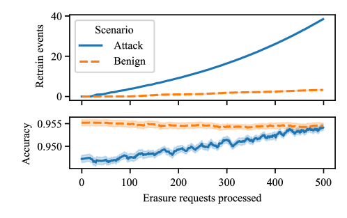
Figure 1: Number of times retraining is triggered as a function of the number of poisoned erasure requests processed. After processing 500 requests, all poisoned instances are erased and only clean data remains.

Transferability.

We investigate whether the attack transfers if surrogate data is used to craft the attack in place of the defender’s training data. This corresponds to the grey-box setting described in Sec. 2.3. Table 5 shows that the attack transfers well—there is very little difference in the retrain interval in the grey- versus white-box settings.

Table 5: Effectiveness of the attack in white-box versus grey-box settings.

Dataset	Retrain interval
	Surrogate data (Grey-box)	Training data (White-box)
MNIST	19.0	18.5
Binary-MNIST	7.88	8.15

Varying datasets.

Most of the results reported above are for Binary-MNIST. Table 6 reports results for other datasets described in Sec. 4.1. While the results are qualitatively similar across datasets, we note some variance in attack effectiveness—depending on the dataset we observe a reduction in the retrain interval of 67–94%. The size of each dataset is likely a factor, since a model trained on more data is less sensitive to individual instances and more difficult to attack. We also expect the $\ell_{1}$-bounded perturbations are likely to have a different impact depending on the characteristics of the data. For instance, Fashion-MNIST has a wider variation of intensities across all pixels compared to MNIST, which may make $\ell_{1}$-bounded perturbations less effective.

Table 6: Effectiveness of the attack for various datasets.

Dataset	Accuracy		Retrain interval
	Benign	Attack	Benign	Attack	% $\downarrow$
MNIST	0.867	0.867	71.6	18.5	74.1
Binary-MNIST	0.954	0.954	132	8.15	93.8
Fashion-MNIST	0.756	0.756	119	38.9	67.5
HAR	0.838	0.836	42.2	8.95	78.8

5 Related Work

Machine unlearning.

Recent interest in efficient data erasure for learned models was spawned by [11], who were motivated by privacy and security applications. They coined the term “machine unlearning” and proposed a strict definition—requiring that an unlearning algorithm return a model identical to one retrained from scratch on the remaining data. Efficient unlearning algorithms are known for some canonical models under this definition, including linear regression [12, 28], naive Bayes and non-parametric models such as $k$-nearest neighbors [42]. These algorithms are immune to our attack since they compute updates in closed form with data-independent running times.

A strict definition of unlearning has proven difficult to satisfy for general models. One solution has been to design new models or adapt existing ones with unlearning efficiency in mind. Examples of such models include ensembles of randomized decision trees [43], variants of $k$-means clustering [22], and a modeling framework called SISA that takes advantage of data sharding and caching [8].

Others have expanded the scope of unlearning by adopting more relaxed (but still rigorous) definitions. [22] were first to introduce an approximate definition of unlearning—requiring that it be statistically indistinguishable from retraining. They identified a connection to differential privacy [19] and suggested adversarial robustness as a direction for future work. Subsequent work [26, 40, 45] has adopted similar approximate definitions to provide certified unlearning guarantees for strongly-convex learning problems. [40] and [45] study asymptotic time complexity, however they do not test their methods empirically and they rely on data-independent bounds which are too loose in practice according to [26]. Since the approach by [26] is empirically validated, we use it for our proof-of-concept exploit in this paper.

Certified unlearning for non-convex models such as deep neural networks (DNNs) remains elusive. [23, 24] have made some progress in this area based on a notion of approximate unlearning. However, their methods do not guarantee approximate unlearning is satisfied and they require further approximations to scale to DNNs. Since their methods run for a predetermined number of iterations, the running time is data-independent, making them immune to slow-down attacks. However, our slow-down attack may cause damage in a different way—preventing proper data erasure or leaving the unlearned model in an unpredictable state.

While our focus in this paper is on attacking unlearning efficiency, others have considered privacy vulnerabilities. [13] demonstrated that a series of published unlearned models are vulnerable to differencing attacks if not appropriately treated. [27] considered an adaptive unlearning setting, where erasure requests may depend on previously published models. They also demonstrated an attack on the SISA algorithm [8]. [50] considered verification of unlearning—an important privacy feature for users who cannot trust organizations to erase their data.

Adversarial machine learning.

Our work builds on standard methods for data poisoning—a class of attacks that manipulate learned models by modifying or augmenting training data (see survey [44]). Two commonly studied variants of data poisoning are availability attacks, which aim to degrade model test performance (e.g. [6, 39, 33, 46, 59, 32]), and backdoor attacks, which aim to cause misclassification of test-time samples that contain a trigger (e.g. [14, 17, 41]). Unlike these attacks, our attack does not aim to harm test performance—rather the aim is to cause trouble at the unlearning stage. This adds another layer of complexity, as we must account for learning and unlearning to craft an effective attack.

Most work on data poisoning assumes learning is done offline, as we do in this paper. However one could imagine an online scenario, where an organization continually updates a model as new data arrives and old data is erased. There has been some work on data poisoning for online learning [55, 57], however existing work does not account for the ability of an attacker to request that their data be erased.

Our attack also borrows ideas from the adversarial examples literature. The $\ell_{p}$-norm constraints that we impose on the attacker’s perturbations are commonly used to generate adversarial examples [51, 25]. While $\ell_{p}$-norm constraints are easy to work with, they have been criticized for failing to capture perceptual distortion [47], which has lead to work on more effective perturbation constraints [58, 4]. These could be leveraged to enhance our attack.

While adversarial examples are predominantly used for evasion attacks, they have also been deployed for other purposes. [29] showed that techniques for generating adversarial examples can be modified to slow down inference of multi-exit DNNs by a factor of 1.5–5$\times$. This attack is qualitatively similar to ours, in that it targets computation cost, however the formulation is different. While our attack operates at training-time and unlearning-time, the attack by [29] operates at test-time. Other novel applications of adversarial examples include data poisoning [52] and protecting data from being used to train models [30].

6 Discussion

We have demonstrated a broad range of settings where a poisoning attack can be successfully launched against state-of-the-art machine unlearning to significantly undo the advantages of unlearning over full retraining. Our results suggest that theory should incorporate a trade-off between indistinguishability, computational cost, and accuracy. Indeed in parallel work to our own, [40] define “strong” unlearning algorithms as those for which accuracy bounds are independent of the number of unlearning requests $t$, with a computation cost that grows at most logarithmically in $t$. They explore trade-offs for an unlearning algorithm called perturbed gradient descent. However this approach hasn’t been evaluated empirically to our knowledge, and a number of open problems remain.

Future work could apply or extend our methods to attack other unlearning algorithms, beyond those by [26], which were the focus of this paper. We expect this would be easiest for algorithms based on a similar design—e.g. algorithms by [40] and [45] also perturb the original model to find an approximate solution to a strongly-convex learning objective post-erasure. Other unlearning algorithms, such as [22]’s algorithm for k-means clustering, are also vulnerable to slow-down attacks, however crafting poisons to trigger retraining would be more difficult due to non-differentiability of the cost function. If certified unlearning algorithms are developed for deep models in the future, then assessing the impact of slow-down attacks in that setting—where data and models are typically at a much larger scale—would also be of immense interest.

Another direction suggested by our work is counter measures against slow-down attacks on unlearning. One might adopt an unlearning algorithm that never resorts to retraining from scratch [23]. Such an algorithm might still require more computational effort to remove poisoned examples than benign examples, exposing a similar attack surface. It is also unclear whether such an algorithm could maintain a form of indistinguishability indefinitely.

One might seek to filter out poisoned examples so they never need to be unlearned. This might involve off-the-shelf anomaly detection methods, however poisoned examples are notoriously difficult to detect when they are crafted as small perturbations to clean examples. [38] for instance, have explored detection of adversarial perturbations. Alternatively, one could filter out examples with a large influence (which the attacker is trying to artificially inflate in our attack), however some clean examples have a naturally large influence.

Another approach would be a robust model that is less sensitive to individual examples. Directions for achieving this include: increasing the degree of regularization, introducing noise, adversarial training, and using more training data. However, like their analogues in existing adversarial learning research, these mitigations tend to harm accuracy.

Appendix A Technical details for PGD

In this appendix, we present algorithms and discuss technical considerations for our PGD-based solution to the optimization problem in (8a)–(8b). Our implementation of PGD is summarized in Alg. 3, which calls sub-routines for backtracking line search (Alg. 4) and the projection operator (Alg. 5).

1:procedure PGD($\mathbf{X}_{0}$)

2:     $\mathbf{X}_{\mathrm{psn}}\leftarrow X_{0}$

3:     for $i\in\{1,\ldots,n_{\mathrm{pgd}}\}$ do

4:         $\mathbf{G}\leftarrow\nabla f(\mathbf{X}_{\mathrm{psn}})$ $\triangleright$ Compute gradient

5:         $\Delta\mathbf{X}_{\mathrm{psn}}\leftarrow\begin{bmatrix}\frac{G_{1\cdot}}{\|G_{1\cdot}\|_{2}}\\ \vdots\\ \frac{G_{m\cdot}}{\|G_{m\cdot}\|_{2}}\end{bmatrix}$ $\triangleright$ Normalize gradient

6:         $\eta\leftarrow\textsc{BLS}(\eta_{0},\mathbf{X}_{\mathrm{psn}},\Delta\mathbf{X}_{\mathrm{psn}},\mathbf{G})$ $\triangleright$ Get step size

7:         $\mathbf{X}_{\mathrm{psn}}\leftarrow\mathbf{X}_{\mathrm{psn}}-\eta\Delta\mathbf{X}_{\mathrm{psn}}$ $\triangleright$ Descent step

8:         $\mathbf{X}_{\mathrm{psn}}\leftarrow\textsc{Proj}(\mathbf{X}_{\mathrm{psn}})$ $\triangleright$ Project step

9:     end for

10:     return $\mathbf{X}_{\mathrm{psn}}$

11:end procedure

Algorithm 3 Projected gradient descent with backtracking line search and gradient normalization.

A.1 Computing gradients

In line 4 of Alg. 3 we compute the gradient of the objective $f$ with respect to the poisoned features $\mathbf{X}_{\mathrm{psn}}$. This is nontrivial since we need to propagate gradients through $\hat{\bm{\mathrm{\theta}}}(D)$, which is implemented as an iterative optimization algorithm. Naïvely applying automatic differentiation to compute $\partial\hat{\bm{\mathrm{\theta}}}/\partial\mathbf{X}_{\mathrm{psn}}$ would require unrolling loops in the optimization algorithm. Fortunately, we can tackle the computation more efficiently using the implicit function theorem [5, Proposition A.25]. Assuming the optimization algorithm runs to convergence, the solution $\hat{\bm{\mathrm{\theta}}}$ satisfies $\nabla_{\bm{\mathrm{\theta}}}R(\hat{\bm{\mathrm{\theta}}};D)=0$. Applying the implicit function theorem on $q(\hat{\bm{\mathrm{\theta}}},\mathbf{X}_{\mathrm{psn}})=\nabla_{\bm{\mathrm{\theta}}}R(\hat{\bm{\mathrm{\theta}}};D)$ gives

$$\frac{\partial\hat{\bm{\mathrm{\theta}}}}{\partial\mathbf{X}_{\mathrm{psn}}}=-[\mathrm{J}_{\bm{\mathrm{\theta}}}q(\hat{\bm{\mathrm{\theta}},\mathbf{X}_{\mathrm{psn}}})]^{-1}\cdot\mathrm{J}_{\mathbf{X}_{\mathrm{psn}}}q(\hat{\bm{\mathrm{\theta}}},\mathbf{X}_{\mathrm{psn}})$$ (13)

where $\mathrm{J}$ is the Jacobian operator. This expression be used to implement a custom gradient for $\hat{\bm{\mathrm{\theta}}}(D)$ in automatic differentiation frameworks such as PyTorch and JAX.

A.2 Controlling the step size

Vanilla gradient descent with a fixed step size tends to converge slowly for this problem. In particular, we observe overshooting when the iterates approach a local optimizer near the boundary of the feasible region. To avoid this behavior, we control the step size by normalizing the gradient row-wise (line 5 in Alg. 3) and applying a backtracking line search (line 6, pseudocode given in Alg. 4). This yields good solutions to (8a)–(8b) in as few as $n_{\mathrm{pgd}}=10$ descent steps. We note that the signed gradient has been used as alternative to the gradient when generating adversarial examples [25, 36]. Both are reasonable approaches—which is more effective likely depends on the geometry of the problem [3].

1:procedure BLS($\eta,\mathbf{X},\Delta\mathbf{X},\mathbf{G}$)

2:     $t\leftarrow c\langle\mathbf{G},\Delta\mathbf{X}\rangle_{F}$ $\triangleright$ Frobenius inner prod.

3:     $\tilde{\mathbf{X}}\leftarrow\mathbf{X}-\eta\Delta\mathbf{X}$

4:     while $f(\mathbf{X})-f(\tilde{\mathbf{X}})<\eta t$ do

5:         $\eta\leftarrow\tau\eta$ $\triangleright$ Reduce step size

6:         $\tilde{\mathbf{X}}\leftarrow\mathbf{X}-\eta\Delta\mathbf{X}$

7:     end while

8:     return $\eta$

9:end procedure

Algorithm 4 Backtracking line search for Alg. 3. Following [2] we set $\tau=c=\frac{1}{2}$.

A.3 Projection operator

PGD depends crucially on an efficient implementation of the projection operator

$$\textsc{Proj}(\mathbf{X}_{\mathrm{psn}})=\arg\min_{\mathbf{X}\in\Omega}\|\mathbf{X}_{\mathrm{psn}}-\mathbf{X}\|_{F}$$ (14)

where $\Omega=\bigcap_{j=1}^{J}\Omega_{j}$ and $\Omega_{j}=\{\mathbf{X}_{\mathrm{psn}}\in\mathbb{R}^{m\times d}:g_{j}(D_{\mathrm{psn}})\leq 0\}$ is the set that satisfies the $j$-th inequality constraint. Since $\Omega_{j}$ is convex by (7), we can solve (14) using Dykstra’s algorithm. It finds an asymptotic solution by recursively projecting onto each convex set $\Omega_{j}$. Pseudocode for Dykstra’s algorithm is provided in Alg. 5, based on the stopping condition by [7]. Note that it calls the projection operator $\Pi_{j}$ onto $\Omega_{j}$, which can be implemented efficiently for the norm-ball constraints in (7). For instance, [18] provides a linear-time projection algorithm onto the $\ell_{1}$-ball.

1:procedure Proj($\mathbf{X}$)

2:     $\mathbf{Y}_{j}\leftarrow\mathbf{0}^{\top}$ $\triangleright$ Initialize increments

3:     $c_{I}=\infty$

4:     while $c_{I}\geq\psi\wedge i<n_{\mathrm{proj}}$ do

5:         $c_{I}\leftarrow 0;\ i\leftarrow i+1$

6:         for $j\in\{1,\ldots,J\}$ do

7:              $\tilde{\mathbf{Y}}\leftarrow\mathbf{Y}_{j}$

8:              $\mathbf{Z}\leftarrow\mathbf{X}-\tilde{\mathbf{Y}}$

9:              $\mathbf{X}\leftarrow\Pi_{j}(\mathbf{Z})$ $\triangleright$ Update iterate

10:              $\mathbf{Y}_{j}\leftarrow\mathbf{X}-\mathbf{Z}$ $\triangleright$ Update increment

11:              $c_{I}\leftarrow c_{I}+\|\tilde{\mathbf{Y}}-\mathbf{Y}_{j}\|_{F}^{2}$ $\triangleright$ Update stopping cond.

12:         end for

13:     end while

14:     return $\mathbf{X}$

15:end procedure

Algorithm 5 Projection operator onto the intersection of $J$ convex sets $\Omega=\bigcap_{j=1}^{J}\Omega_{j}$ based on Dykstra’s algorithm [7]. Here $\psi$ is the tolerance for the stopping condition, $n_{\mathrm{proj}}$ is the maximum number of iterations, and $\Pi_{j}$ is the projection operator onto $\Omega_{j}$.

Appendix B Experimental details

In this appendix, we provide further details about the experiments presented in Sec. 4.

B.1 Implementation and hardware

We implemented our experiments in JAX version 0.2.5 [9] owing to its advanced automatic differentiation features. Experiments were run on a HPC cluster using a NVIDIA P100 GPU with 12GB GPU memory and 32GB CPU memory. We repeated all simulations 100 times and reported mean values to account for multiple sources of randomness.

B.2 Learning algorithm

We assumed the organization and the attacker both used L-BFGS [35] to fit their models. We stopped L-BFGS after a maximum of 1000 iterations or when the $\ell_{\infty}$-norm of the gradient reached a tolerance of $10^{-6}$—whichever occurred first. For the multi-class case, we used a one-vs-rest strategy, since the learning problem (1) does not allow for vector-valued labels. Inputs to the model were normalized by their $\ell_{2}$-norm to ensure the condition for (4) was satisfied.

B.3 Attacker settings

We configured the attacker to run PGD (see Appendix A) for $n_{\mathrm{pdg}}=10$ iterations using an initial step size $\eta_{0}=d/10$. The projection operator was run with a tolerance of $\psi=10^{-6}$ for a maximum of $n_{\mathrm{proj}}=50$ iterations.

The fraction of poisoned instances in the training set $|D_{\mathrm{psn}}|/|D|$ varied across the experiments (see Table 7), but was always less than 1%. For a given experiment, the number of poisoned instances $|D_{\mathrm{psn}}|$ was set to be large enough so that only poisoned instances were unlearned.

Unless otherwise specified, we used the influence norm cost function (11) and ignored model dependence on the poisoned data. We found these settings gave a reasonable trade-off between attack time and poison quality.

Table 7: Number of poisoned instances $|D_{\mathrm{psn}}|$ for experiments in Sec. 4.2.

Dataset	$\lambda$	$\sigma$	$p$	$r$	Cost function	$|D_{\mathrm{psn}}|$
Fashion-MNIST	$10^{-3}$	10	1	$d/20$	Influence	50
HAR	$10^{-3}$	10	1	$d/20$	Influence	20
MNIST	$10^{-3}$	10	1	$d/20$	Influence	40
Binary-MNIST	$10^{-2}$	10	1	$d/20$	Influence	600
Binary-MNIST	$10^{-3}$	10	1	$d/20$	Influence	20
Binary-MNIST	$10^{-3}$	10	1	$d/20$	Gradient	20
Binary-MNIST	$10^{-3}$	10	1	$d/20$	GRNB	20
Binary-MNIST	$10^{-3}$	10	1	$d/200$	Influence	90
Binary-MNIST	$10^{-3}$	10	1	$d/2$	Influence	20
Binary-MNIST	$10^{-3}$	10	1	$d$	Influence	10
Binary-MNIST	$10^{-3}$	10	$\infty$	$1/20$	Influence	100
Binary-MNIST	$10^{-3}$	10	$\infty$	$1/10$	Influence	60
Binary-MNIST	$10^{-3}$	10	$\infty$	$1/2$	Influence	10
Binary-MNIST	$10^{-3}$	10	$\infty$	1	Influence	10
Binary-MNIST	$10^{-4}$	10	1	$d/20$	Influence	5
Binary-MNIST	$10^{-5}$	10	1	$d/20$	Influence	1
Binary-MNIST	$10^{-2}$	1	1	$d/20$	Influence	60
Binary-MNIST	$10^{-3}$	1	1	$d/20$	Influence	5
Binary-MNIST	$10^{-4}$	1	1	$d/20$	Influence	1
Binary-MNIST	$10^{-5}$	1	1	$d/20$	Influence	1

We applied $J=2$ inequality constraints of the form given in (7):

$$g_{1}(D_{\mathrm{psn}}) =\sup_{\bm{\mathrm{x}}\in\mathrm{rows}(\mathbf{X}_{\mathrm{psn}}-\mathbf{V}_{1})}\left\|\bm{\mathrm{x}}\right\|_{\infty}-r_{1} \leq 0,$$

$$g_{2}(D_{\mathrm{psn}}) =\sup_{\bm{\mathrm{x}}\in\mathrm{rows}(\mathbf{X}_{\mathrm{psn}}-\mathbf{X}_{\mathrm{ref}})}\left\|\bm{\mathrm{x}}\right\|_{p}-r \leq 0.$$

The first constraint ensures features are within valid ranges. For MNIST and Fashion-MNIST, we set $\mathbf{V}_{1}=\mathbf{0}_{m,d}$ (zero matrix) and $r_{1}=1$ to ensure pixel intensities were in the range $[0,1]$. For HAR, we set $\mathbf{V}_{1}=-\mathbf{1}_{m,d}$ (all-ones matrix) and $r_{1}=2$ to ensure features were in the range $[-1,1]$. The second constraint bounds the attacker’s perturbations to the clean reference features $\mathbf{X}_{\mathrm{ref}}$. Unless otherwise specified we set $p=1$ and $r=d/20$.

B.4 Organization settings

We set $\epsilon=1$ and $\delta=10^{-4}$ to achieve a reasonable erasure guarantee. By default, we applied moderate regularization with $\lambda=10^{-3}$ and perturbed the objective with noise of magnitude $\sigma=10$. These settings were found to balance model accuracy and unlearning efficiency in a benign setting (see Table 2).

Appendix C Additional results on long-term effectiveness

This appendix includes additional experimental results on the long-term effectiveness of our attack. In the previous results (Sec. 4.2 excluding Figure 1), we measured the effectiveness of our attack in terms of the retrain interval—the number of erasure requests handled before full retraining is triggered for the first time. We now consider the impact of our attack when erasure requests continue to be processed, even after retraining occurs potentially many times. For these experiments we report the retrain frequency—the fraction of erasure requests that trigger retraining—as a measure of effectiveness. A higher retrain frequency means our attack is more effective at increasing the computational cost of unlearning.

We report the retrain frequency averaged over 500 erasure requests, where all 500 requests are poisoned (i.e., we fix $|D_{\mathrm{psn}}|=500$). This yields precise estimates for most experiments, where the average retrain interval is significantly less than 500 and the retrain frequency is significantly larger than 1.

Table 8 reports long-term effectiveness as a function of the model sensitivity parameters, similarly to Table 2. We observe that our attack yields the largest gains in retrain frequency when retraining would be infrequent in a benign setting. In other words, our attack is most effective in the regime where unlearning would normally be most effective. We note that there is some degree of uncertainty in estimates of retrain frequency close to zero—i.e., for $\lambda\geq 10^{-3}$.

We examined the retrain frequency as a function of the perturbation constraint ($p$ and $r$), however we omit the results here as they qualitatively similar to Table 3. Tables 9–11 report results on alternative cost functions, transferability and additional datasets. These results are analogous to Tables 4–6 in the main paper and show similar trends in terms of attack effectiveness.

Table 8: Long-term attack effectiveness on Binary-MNIST as a function of the regularization strength $\lambda$ and magnitude of the objective perturbation $\sigma$. The accuracy is reported for the initial model, prior to processing erasure requests.

$\sigma$	$\lambda$	Accuracy		Retrain frequency (%)
		Benign	Attack	Benign	Attack	% $\uparrow$
1	$10^{-5}$	0.962	0.962	21.7	27.4	26.1
	$10^{-4}$	0.968	0.968	16.3	37.8	132
	$10^{-3}$	0.958	0.952	5.65	53.6	849
	$10^{-2}$	0.927	0.921	0.404	1.88	366
10	$10^{-5}$	0.919	0.917	100	100	-0.01
	$10^{-4}$	0.933	0.928	9.67	26.8	177
	$10^{-3}$	0.955	0.947	0.656	7.69	1070
	$10^{-2}$	0.926	0.920	0	0.132	–

Table 9: Long-term attack effectiveness and computation time for different choices of the cost function.

Cost function	Ignore model dep.	Retrain frequency	Attack time (s)
GRNB (10)	No	7.91	170.5
	Yes	8.05	22.6
Influence norm (11)	No	5.07	62.4
	Yes	7.69	8.84
Gradient norm (12)	No	4.74	21.8
	Yes	4.64	3.87

Table 10: Long-term effectiveness of the attack in white-box versus grey-box settings.

Dataset	Retrain frequency (%)
	Surrogate data (Grey-box)	Training data (White-box)
MNIST	4.63	4.43
Binary-MNIST	7.90	7.69

Table 11: Long-term effectiveness of the attack for various datasets.

Dataset	Initial accuracy		Retrain frequency (%)
	Benign	Attack	Benign	Attack	% $\uparrow$
MNIST	0.867	0.867	1.27	4.43	250
Binary-MNIST	0.955	0.947	0.656	7.69	1070
Fashion-MNIST	0.756	0.755	0.778	2.18	180
HAR	0.837	0.836	2.37	9.37	296

References

- [1] Davide Anguita et al. “A Public Domain Dataset for Human Activity Recognition using Smartphones” In 21st International European Symposium on Artificial Neural Networks, Computational Intelligence and Machine Learning, 2013 URL: https://www.esann.org/sites/default/files/proceedings/legacy/es2013-84.pdf
- [2] Larry Armijo “Minimization of functions having Lipschitz continuous first partial derivatives” In Pacific Journal of Mathematics 16.1, 1966, pp. 1–3 DOI: 10.2140/pjm.1966.16.1
- [3] Lukas Balles, Fabian Pedregosa and Nicolas Le Roux “The Geometry of Sign Gradient Descent”, 2020 arXiv:2002.08056 [cs.LG]
- [4] Vincent Ballet et al. “Imperceptible Adversarial Attacks on Tabular Data”, 2019 arXiv:1911.03274 [stat.ML]
- [5] Dimitri P. Bertsekas “Nonlinear Programming” Athena Scientific, 1999
- [6] Battista Biggio, Blaine Nelson and Pavel Laskov “Poisoning Attacks against Support Vector Machines” In Proceedings of the 29th International Coference on International Conference on Machine Learning, 2012, pp. 1467–1474
- [7] Ernesto G. Birgin and Marcos Raydan “Robust Stopping Criteria for Dykstra’s Algorithm” In SIAM Journal on Scientific Computing 26.4, 2005, pp. 1405–1414 DOI: 10.1137/03060062X
- [8] L. Bourtoule et al. “Machine Unlearning” In 2021 IEEE Symposium on Security and Privacy (SP), 2021, pp. 141–159 DOI: 10.1109/SP40001.2021.00019
- [9] James Bradbury et al. “JAX: composable transformations of Python+NumPy programs”, 2018 URL: http://github.com/google/jax
- [10] California State Legislature “California Consumer Privacy Act of 2018” https://leginfo.legislature.ca.gov/faces/codes_displayText.xhtml?division=3.&part=4.&lawCode=CIV&title=1.81.5, Cal. Civ. Code §1798.100, 2018
- [11] Yinzhi Cao and Junfeng Yang “Towards Making Systems Forget with Machine Unlearning” In 2015 IEEE Symposium on Security and Privacy, 2015, pp. 463–480 DOI: 10.1109/SP.2015.35
- [12] John M. Chambers “Regression Updating” In Journal of the American Statistical Association 66.336, 1971, pp. 744–748
- [13] Min Chen et al. “When Machine Unlearning Jeopardizes Privacy”, 2020 arXiv:2005.02205 [cs.CR]
- [14] Xinyun Chen et al. “Targeted Backdoor Attacks on Deep Learning Systems Using Data Poisoning”, 2017 arXiv:1712.05526 [cs.CR]
- [15] R. Cook and Sanford Weisberg “Characterizations of an Empirical Influence Function for Detecting Influential Cases in Regression” In Technometrics 22.4, 1980, pp. 495–508 DOI: 10.1080/00401706.1980.10486199
- [16] Council of the EU “Regulation (EU) 2016/679 on the protection of natural persons with regard to the processing of personal data and on the free movement of such data, and repealing Directive 95/46/EC (General Data Protection Regulation)” In Official Journal of the European Union L 119, 2016, pp. 1–88
- [17] Jiazhu Dai, Chuanshuai Chen and Yufeng Li “A Backdoor Attack Against LSTM-Based Text Classification Systems” In IEEE Access 7, 2019, pp. 138872–138878 DOI: 10.1109/ACCESS.2019.2941376
- [18] John Duchi, Shai Shalev-Shwartz, Yoram Singer and Tushar Chandra “Efficient Projections onto the -Ball for Learning in High Dimensions” In Proceedings of the 25th International Conference on Machine Learning, 2008, pp. 272–279 DOI: 10.1145/1390156.1390191
- [19] Cynthia Dwork et al. “Our Data, Ourselves: Privacy Via Distributed Noise Generation” In Advances in Cryptology - EUROCRYPT 2006, 2006, pp. 486–503
- [20] Matt Fredrikson, Somesh Jha and Thomas Ristenpart “Model Inversion Attacks That Exploit Confidence Information and Basic Countermeasures” In Proceedings of the 22nd ACM SIGSAC Conference on Computer and Communications Security, 2015, pp. 1322–1333 DOI: 10.1145/2810103.2813677
- [21] FTC “California Company Settles FTC Allegations It Deceived Consumers about use of Facial Recognition in Photo Storage App” https://www.ftc.gov/news-events/press-releases/2021/01/california-company-settles-ftc-allegations-it-deceived-consumers, 2021
- [22] Antonio Ginart, Melody Guan, Gregory Valiant and James Y Zou “Making AI Forget You: Data Deletion in Machine Learning” In Advances in Neural Information Processing Systems 32, 2019
- [23] Aditya Golatkar, Alessandro Achille and Stefano Soatto “Eternal Sunshine of the Spotless Net: Selective Forgetting in Deep Networks” In 2020 IEEE/CVF Conference on Computer Vision and Pattern Recognition (CVPR), 2020, pp. 9301–9309 DOI: 10.1109/CVPR42600.2020.00932
- [24] Aditya Golatkar, Alessandro Achille and Stefano Soatto “Forgetting Outside the Box: Scrubbing Deep Networks of Information Accessible from Input-Output Observations” In Computer Vision – ECCV 2020, 2020, pp. 383–398
- [25] Ian J. Goodfellow, Jonathon Shlens and Christian Szegedy “Explaining and Harnessing Adversarial Examples”, 2015 arXiv:1412.6572 [stat.ML]
- [26] Chuan Guo, Tom Goldstein, Awni Hannun and Laurens Van Der Maaten “Certified Data Removal from Machine Learning Models” In Proceedings of the 37th International Conference on Machine Learning 119, 2020, pp. 3832–3842
- [27] Varun Gupta et al. “Adaptive Machine Unlearning”, 2021 arXiv:2106.04378 [cs.LG]
- [28] Lars Kai Hansen and Jan Larsen “Linear unlearning for cross-validation” In Advances in Computational Mathematics 5, 1996, pp. 269–280 DOI: 10.1007/BF02124747
- [29] Sanghyun Hong, Yigitcan Kaya, Ionu-Vlad Modoranu and Tudor Dumitras “A Panda? No, It’s a Sloth: Slowdown Attacks on Adaptive Multi-Exit Neural Network Inference” In International Conference on Learning Representations, 2021 URL: https://openreview.net/forum?id=9xC2tWEwBD
- [30] Hanxun Huang et al. “Unlearnable Examples: Making Personal Data Unexploitable” In International Conference on Learning Representations, 2021 URL: https://openreview.net/forum?id=iAmZUo0DxC0
- [31] Ling Huang et al. “Adversarial Machine Learning” In Proceedings of the 4th ACM Workshop on Security and Artificial Intelligence, 2011, pp. 43–58 DOI: 10.1145/2046684.2046692
- [32] W. Huang et al. “MetaPoison: Practical General-purpose Clean-label Data Poisoning” In Advances in Neural Information Processing Systems 33, 2020, pp. 12080–12091
- [33] Pang Wei Koh and Percy Liang “Understanding Black-Box Predictions via Influence Functions” In Proceedings of the 34th International Conference on Machine Learning - Volume 70, 2017, pp. 1885–1894
- [34] Yann LeCun, Léon Bottou, Yoshua Bengio and Patrick Haffner “Gradient-based learning applied to document recognition” In Proceedings of the IEEE 86.11, 1998, pp. 2278–2324 DOI: 10.1109/5.726791
- [35] Dong C. Liu and Jorge Nocedal “On the limited memory BFGS method for large scale optimization” In Mathematical Programming 45.1, 1989, pp. 503–528 DOI: 10.1007/BF01589116
- [36] Aleksander Madry et al. “Towards Deep Learning Models Resistant to Adversarial Attacks” In International Conference on Learning Representations, 2018 URL: https://openreview.net/forum?id=rJzIBfZAb
- [37] Shike Mei and Xiaojin Zhu “Using Machine Teaching to Identify Optimal Training-Set Attacks on Machine Learners” In Proceedings of the Twenty-Ninth AAAI Conference on Artificial Intelligence, 2015, pp. 2871–2877
- [38] Jan Hendrik Metzen, Tim Genewein, Volker Fischer and Bastian Bischoff “On Detecting Adversarial Perturbations” In Proceedings of 5th International Conference on Learning Representations (ICLR), 2017
- [39] Luis Muñoz-González et al. “Towards Poisoning of Deep Learning Algorithms with Back-Gradient Optimization” In Proceedings of the 10th ACM Workshop on Artificial Intelligence and Security, 2017, pp. 27–38 DOI: 10.1145/3128572.3140451
- [40] Seth Neel, Aaron Roth and Saeed Sharifi-Malvajerdi “Descent-to-Delete: Gradient-Based Methods for Machine Unlearning” In Proceedings of the 32nd International Conference on Algorithmic Learning Theory 132, 2021, pp. 931–962 URL: https://proceedings.mlr.press/v132/neel21a.html
- [41] Aniruddha Saha, Akshayvarun Subramanya and Hamed Pirsiavash “Hidden Trigger Backdoor Attacks” In Proceedings of the AAAI Conference on Artificial Intelligence 34.7, 2020, pp. 11957–11965 DOI: 10.1609/aaai.v34i07.6871
- [42] Sebastian Schelter ““Amnesia” – Machine Learning Models That Can Forget User Data Very Fast” In Online Proceedings of the 10th Conference on Innovative Data Systems Research, 2020
- [43] Sebastian Schelter, Stefan Grafberger and Ted Dunning “HedgeCut: Maintaining Randomised Trees for Low-Latency Machine Unlearning” In Proceedings of the 2021 International Conference on Management of Data, 2021, pp. 1545–1557 DOI: 10.1145/3448016.3457239
- [44] Avi Schwarzschild et al. “Just How Toxic is Data Poisoning? A Unified Benchmark for Backdoor and Data Poisoning Attacks” In Proceedings of the 38th International Conference on Machine Learning 139, 2021, pp. 9389–9398
- [45] Ayush Sekhari, Jayadev Acharya, Gautam Kamath and Ananda Theertha Suresh “Remember What You Want to Forget: Algorithms for Machine Unlearning”, 2021 arXiv:2103.03279 [cs.LG]
- [46] Ali Shafahi et al. “Poison Frogs! Targeted Clean-Label Poisoning Attacks on Neural Networks” In Proceedings of the 32nd International Conference on Neural Information Processing Systems, 2018, pp. 6106–6116
- [47] Mahmood Sharif, Lujo Bauer and Michael K. Reiter “On the Suitability of Lp-Norms for Creating and Preventing Adversarial Examples” In Proceedings of the IEEE Conference on Computer Vision and Pattern Recognition (CVPR) Workshops, 2018
- [48] Juncheng Shen, Xiaolei Zhu and De Ma “TensorClog: An Imperceptible Poisoning Attack on Deep Neural Network Applications” In IEEE Access 7, 2019, pp. 41498–41506 DOI: 10.1109/ACCESS.2019.2905915
- [49] Reza Shokri, Marco Stronati, Congzheng Song and Vitaly Shmatikov “Membership Inference Attacks Against Machine Learning Models” In 2017 IEEE Symposium on Security and Privacy (SP), 2017, pp. 3–18 DOI: 10.1109/SP.2017.41
- [50] David Marco Sommer, Liwei Song, Sameer Wagh and Prateek Mittal “Towards Probabilistic Verification of Machine Unlearning”, 2020 arXiv:2003.04247 [cs.CR]
- [51] Christian Szegedy et al. “Intriguing properties of neural networks”, 2014 arXiv:1312.6199 [cs.CV]
- [52] Lue Tao et al. “Provable Defense Against Delusive Poisoning”, 2021 arXiv:2102.04716 [cs.LG]
- [53] UK ICO “Guidance on the AI auditing framework: Draft guidance for consultation” Version 1.0, https://ico.org.uk/media/about-the-ico/consultations/2617219/guidance-on-the-ai-auditing-framework-draft-for-consultation.pdf, 2020
- [54] Michael Veale, Reuben Binns and Lilian Edwards “Algorithms that remember: model inversion attacks and data protection law” In Philosophical Transactions of the Royal Society A: Mathematical, Physical and Engineering Sciences 376.2133, 2018, pp. 20180083
- [55] Yizhen Wang and Kamalika Chaudhuri “Data Poisoning Attacks against Online Learning”, 2018 arXiv:1808.08994 [cs.LG]
- [56] Han Xiao, Kashif Rasul and Roland Vollgraf “Fashion-MNIST: a Novel Image Dataset for Benchmarking Machine Learning Algorithms”, 2017 arXiv:1708.07747 [cs.LG]
- [57] Xuezhou Zhang, Xiaojin Zhu and Laurent Lessard “Online Data Poisoning Attacks” In Proceedings of the 2nd Conference on Learning for Dynamics and Control 120, 2020, pp. 201–210
- [58] Zhengyu Zhao, Zhuoran Liu and Martha Larson “Towards Large Yet Imperceptible Adversarial Image Perturbations With Perceptual Color Distance” In Proceedings of the IEEE/CVF Conference on Computer Vision and Pattern Recognition (CVPR), 2020
- [59] Chen Zhu et al. “Transferable Clean-Label Poisoning Attacks on Deep Neural Nets” In Proceedings of the 36th International Conference on Machine Learning 97, 2019, pp. 7614–7623