Deep Spiking Neural Networks
with Resonate-and-Fire Neurons

Abstract

In this work, we explore a new Spiking Neural Network (SNN) formulation with Resonate-and-Fire (RAF) neurons (Izhikevich, 2001) trained with gradient descent via back-propagation. The RAF-SNN, while more biologically plausible, achieves performance comparable to or higher than conventional models in the Machine Learning literature across different network configurations, using similar or fewer parameters. Strikingly, the RAF-SNN proves robust against noise induced at testing/training time, under both static and dynamic conditions. Against CNN on MNIST, we show $25\%$ higher absolute accuracy with $\mathcal{N}(0,0.2)$ induced noise at testing time. Against LSTM on N-MNIST, we show $70\%$ higher absolute accuracy with $20\%$ induced noise at training time.

1 Introduction

Artificial intelligence traces many of its roots back to research in neuroscience and psychology—research seeking to understand the human brain, from the neuronal to the behavioral level. For example, Convolutional Neural Networks (CNNs) were inspired by the hierarchical feed-forward structure of the visual cortex (Hubel & Wiesel, 1968; Fukushima, 1980). Reinforcement Learning (RL) branched out from psychology research on animal conditioning (Rescorla & Wagner, 1972). Interestingly, there are many instances where AI progress has inspired new brain theories that were later empirically verified. For example, RL research inspired a reward-based learning theory of dopaminergic function (Schultz et al., 1997). While deep CNNs trained on natural images were shown to reproduce neurophysiological patterns observed in animals (Lindsay, 2020). Both fields have mutually benefited one another in what has been recently called “a virtuous circle” (Hassabis et al., 2017).

In this light, the scientific community has been exploring Spiking Neural Networks (SNNs). SNNs employ simplified models that approximate neuronal mechanisms we believe the brain uses to process discrete spatio-temporal events (the spikes). One prominent such model is the Leaky-Integrate-and-Fire (LIF) neuron. In LIF, the neuron integrates the inputs over time, firing when the potential passes a set threshold. Hardware architectures have been developed to exploit this event-based behaviour (Merolla et al., 2014; Ankit et al., 2017; Davies et al., 2018). Their results are auspicious for achieving ultra-low power processing of event-based data streams. For example, in deep learning architectures with spiking neurons, it was observed that the number of spikes drops significantly at deeper layers, reducing the computation requirements for neuromorphic hardware (Rueckauer et al., 2017; Sengupta et al., 2019). A caveat of these approaches is that the neuron model utilized (the LIF neuron) can not reproduce relevant features of cortical neurons (Izhikevich, 2001).

Towards overcoming this limitation, we consider a novel SNN with a more biologically plausible neuron model: the Resonate-and-Fire (RAF) model (Izhikevich, 2001). The RAF neuron can model more neurodynamics given its characteristic as a resonator model, and research has shown it to replicate biological neural data, despite its simplicity compared to other resonator neuronal models (Torikai & Hishiki, 2009; Pauley et al., 2018).

2 Methods and Experiments

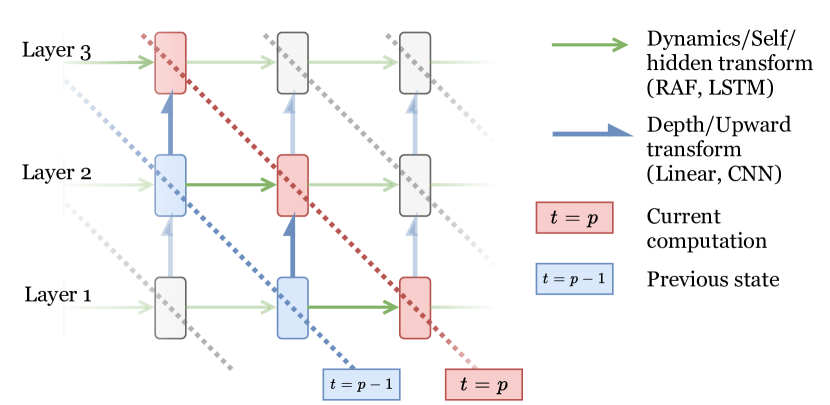
(a)

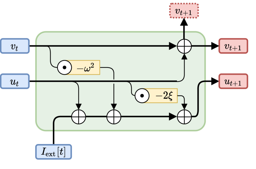
(b)

Figure 1: (a) The forward pass of the (Upward) RAF-SNN, unrolled in time. (b) The RAF² neuron in the style of conventional recurrent cells such as the LSTM.

Figure 1(a) visualizes an Upward² RAF-SNN unrolled in time. A time unit $dt$ is defined as a single step forward for each cell in the network. Thus, notice that input at $t=0$ propagates through the network such that the corresponding output would be at $t=L-1$, for depth $L$, not at $t=0$. This formulation is useful for dealing with the dynamical system of the RAF neuron, but is otherwise functionally equivalent to conventional RNN cells, like the LSTM, with the caveat that observed outputs are shifted in time by $+L-1$. The self-transforms ${\bm{v}}^{\ell}_{t-1}\mapsto{\bm{v}}^{\ell}_{t}$ (green) correspond to ${\bm{h}}^{\ell}_{\tau-1}\mapsto{\bm{h}}^{\ell}_{\tau}$. The depth-transforms ${\bm{v}}^{\ell-1}_{t-1}\mapsto{\bm{v}}^{\ell}_{t}$ (blue) correspond to ${\bm{h}}^{\ell-1}_{\tau}\mapsto{\bm{h}}^{\ell}_{\tau}$, and so on.

2.1 The RAF Neuron Model

Equation 1 shows the RAF neuron model. It describes the dynamics of the membrane potential of a neuron with the equation of motion of a forced, damped harmonic oscillator:

$$\frac{d^{2}v}{dt^{2}}+2\xi\frac{dv}{dt}+\omega^{2}v =I_{\text{ext}}[t]$$ (1)

$$V_{t} \approx V_{t-1}+dt\odot u_{t-1},$$ (2)

$$u_{t} \approx u_{t-1}+dt\odot\left(I_{\text{ext}}-2\xi u_{t-1}-\omega^{2}V_{t-1}\right).\dot{V} =u_{t-1},$$ (3)

$$\dot{u} =I_{\text{ext}}+-\omega^{2}V_{t-1}-2\xi u_{t-1},$$ (4)

$$x_{t} =x_{t-1}+\dot{x}dt\quad\forall x\in\{u,V\}.$$ (5)

where $v$ is the membrane potential, $\xi$ is the damping factor, $\omega$ is the natural frequency, and $I_{\text{ext}}$ is any external current to the neuron (i.e., the weighted summation of pre-synaptic spikes).

2.2 Datasets

We evaluate our formulation on both the static and the dynamic (or neuromorphic) versions of the MNIST dataset (LeCun et al., 1998; Orchard et al., 2015). The static version comprises $28\times 28$ gray-scale images of hand written digits, while the neuromorphic version (“N-MNIST”) was derived from the static dataset by panning and tilting a Dynamic Vision Sensor (DVS) (Lichtsteiner et al., 2008) in front of a screen displaying the digits. Each sample consists of a $300\text{\,}\mathrm{ms}$ period of ON and OFF events that represent increases or decreases in pixel intensity. The data-stream is pre-processed to be a sequence of $34\times 34\times 2$ tensors, similar to Lee et al. (2016), with a sampling time of $10\text{\,}\mathrm{ms}$.

2.3 Experimental Setup

Models

We consider $4$ models: RAF vs. LSTM on N-MNIST, and RAF-CNN vs. CNN on MNIST. RAF models follow the recurrence in Equations 8, 9 & 10. Beyond that, the RAF-CNN substitutes a convolutional layer for the linear at $f^{(\ell)}(s)$. Architecture parameters (e.g. depth and width) are matched for LSTM & RAF networks, and CNN & RAF-CNN. Further details in Appendix A.1.

Poisson Encoding

For the RAF-CNN model, the static inputs are first encoded as Poisson-distributed spike trains where the intensity of each pixel defines the event rate—a standard practice for SNNs (O’Connor et al., 2013; Diehl et al., 2015).

Perturbing Images

In the static case, we add Gaussian noise of a certain std-dev to the pixel values before Poisson Encoding. In the dynamic case, we flip individual binary pixels with some probability $p$ at every time step.

Optimization

Since SNNs deal with discontinuous spikes (binary activations), we employ the method proposed by Yanguas-Gil (2020) to enable training with back-propagation. The forward pass follows Equation 6, while the gradients are based on the smooth approximation in Equation 7:

$$s^{{\ell}j}_{t} =H(v^{{\ell}j}_{t}-\theta^{{\ell}j}),$$ (6)

$$\partial~{}s^{{\ell}j}_{t} =\partial~{}\sigma(\beta^{{\ell}j}(v^{{\ell}j}_{t}-\theta^{{\ell}j})).$$ (7)

where $s^{{\ell}j}_{t}$ is the output spike of neuron $j$ in layer $\ell$ at time $t$, $v^{{\ell}j}_{t}$ is its membrane potential, $\theta^{{\ell}j}$ is the firing threshold, $\beta^{{\ell}j}$ is a regularization parameter (controls the steepness of the sigmoid approximation), $H(\cdot)$ is the Heaviside function, and $\sigma(\cdot)$ is the sigmoid function. Per neuron, $\{\omega,\xi,\theta,\beta\}$ are learnable. Equations 8 & 9 are first-order approximations of Equation 1 in vector form. $f^{(\ell)}(\cdot)$ is a learned forward transform, such as a linear or convolutional layer.

$${\bm{v}}_{t+1} ={\bm{v}}_{t}+dt\odot{\bm{u}}_{t},$$ (8)

$${\bm{u}}_{t+1} ={\bm{u}}_{t}+dt\odot\left({\bm{I}}_{\text{ext}}[t]-2{\bm{\xi}}\odot{\bm{u}}_{t}-{\bm{\omega}}^{2}\odot{\bm{v}}_{t}\right),$$ (9)

$${\bm{I}}_{\text{ext}}^{\ell}[t] =f^{(\ell)}({\bm{s}}_{t}^{\ell-1}).$$ (10)

We use the AdamW optimizer (Loshchilov & Hutter, 2019) with an initial learning rate of $0.01$. The model is trained until the validation accuracy fails to improve for 6 consecutive epochs, where each epoch enumerates the training set in random order. The learning rate is halved when the validation loss does not improve for $2$ epochs. The mini-batch size is $32$. Neuron parameters are initialized by uniform sampling: $\omega\sim\mathcal{U}(0,1.1\times 2\pi)$, $\xi\sim\mathcal{U}(0,2.5)$, $\theta\sim\mathcal{U}(0,2.5)$. While $\beta_{\text{init}}=5$.

Objective Function

In the static case, optimizing the cross-entropy loss on the last observed membrane potential ${v}_{t=\text{last}}$ yields the best results. In the dynamic case, we compute the cross-entropy loss on the number of spikes in the last $15$ time steps as values to the $\mathrm{softmax}$.

3 Results

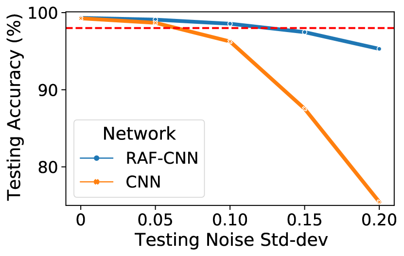
(a)

(b)

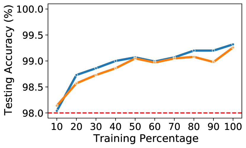
(c)

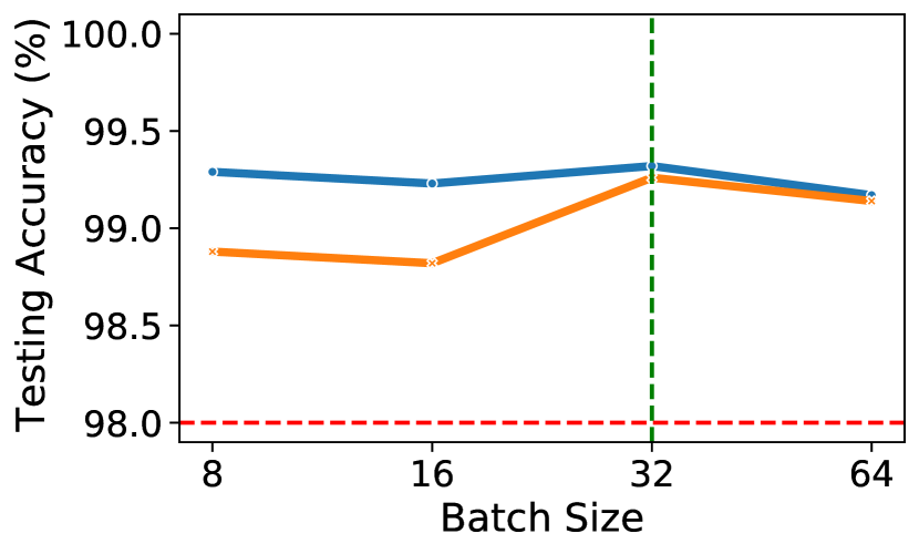
(d)

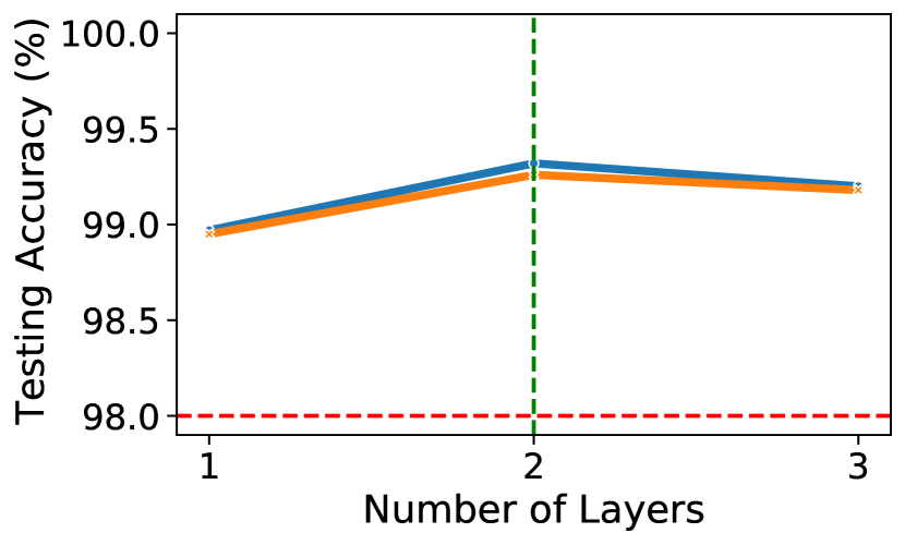
(e)

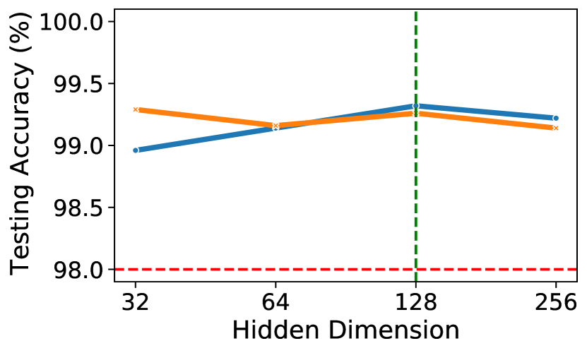
(f)

Figure 2: Test accuracy on the MNIST dataset (static). Comparison of RAF-CNNs vs. CNNs as a function of: (a) Noise std-dev at test, (b) Noise std-dev at train, (c) Training set size, (d) Batch size⁴, (e) Depth⁴, and (f) Width⁴. The red line is a visual anchor at $98\%$ accuracy.

* Each data point is the average of $8$ runs, to account for the probabilistic noise and the Poisson encoder.

In the static (or synthesized) case (Figure 2), we observe model behavior when adding Gaussian noise to the base input images across a range of std-dev values. With up to $\sigma\!=\!0.2$ noise added at testing time for a network trained with clean input: The RAF-CNN maintains performance, while the CNN degrades by up to $25\%$ accuracy. Both networks, however, maintain performance when fed increasingly noisy inputs at training time, as measured on the clean test set. Both networks also present similar performance trajectories when varying the training data size, although the RAF-CNN manages to lead very slightly. In addition, we tested across a range of values for batch size, network width, and depth—both models behaved similarly.

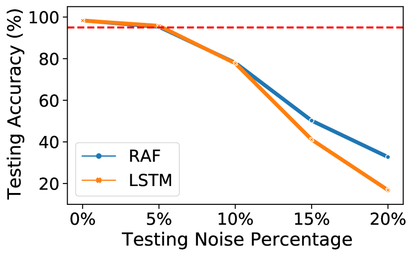
(a)

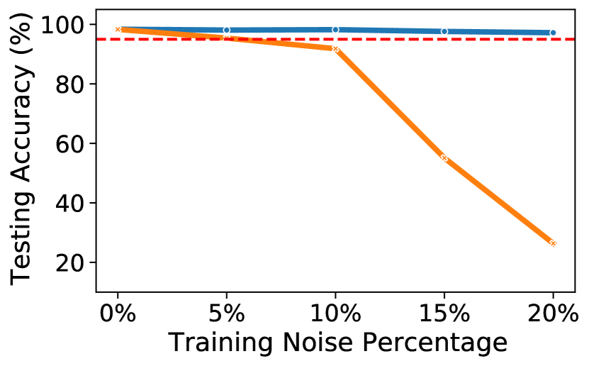
(b)

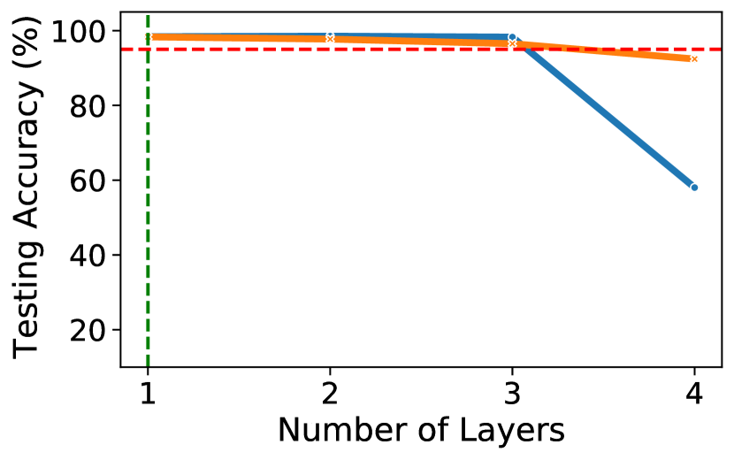
(c)

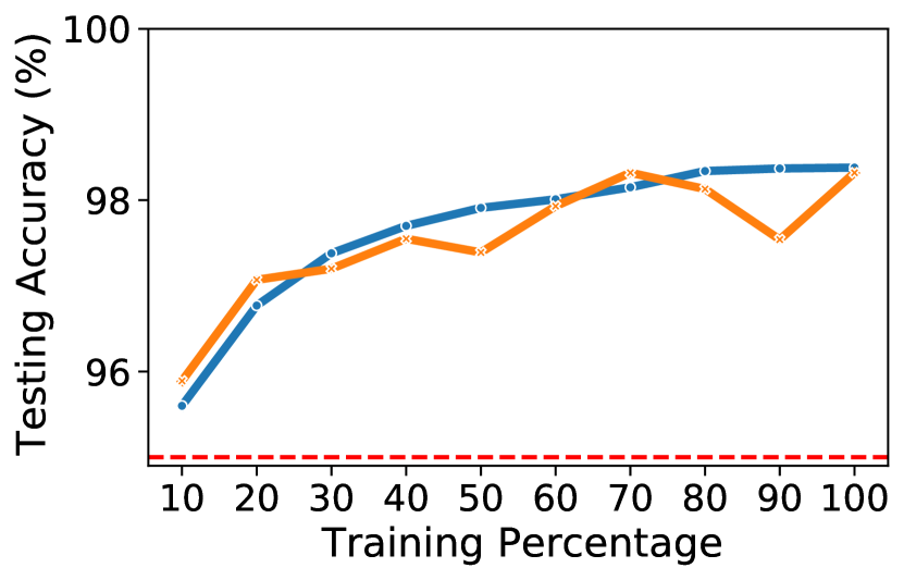
(d)

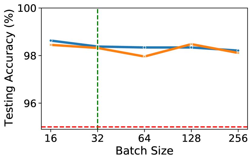
(e)

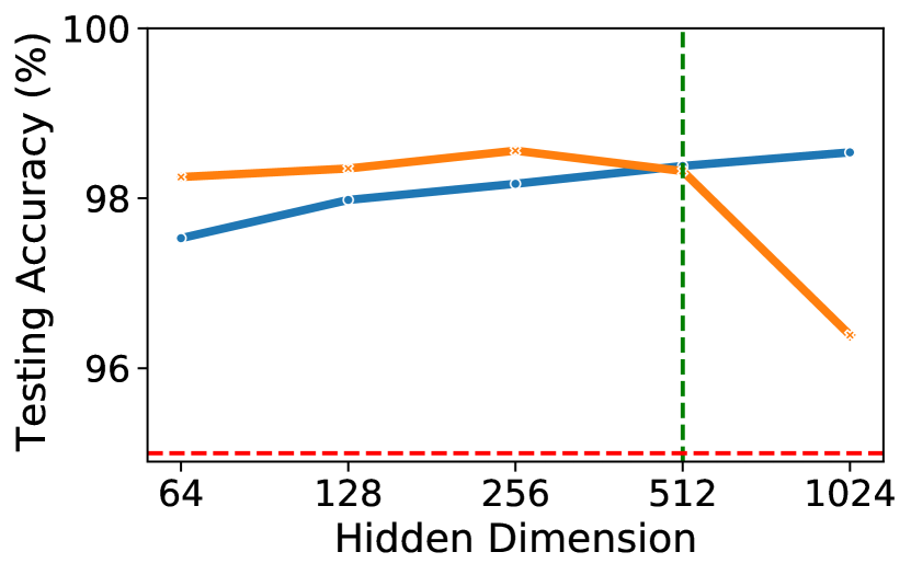
(f)

Figure 3: Test accuracy on the N-MNIST dataset (dynamic). Comparison of RAF vs. LSTM-networks as a function of: (a) Noise $p$ at test, (b) Noise $p$ at train, (c) Network depth, (d) Training set size, (e) Batch size⁴, and (f) Network width⁴. The red line is a visual anchor at $95\%$ accuracy.

In the dynamic (or neuromorphic) case (Figure 3), both the RAF and LSTM degrade as we add more noise at testing time to networks trained with clean input. At $p\!=\!0.2$, The RAF network gets $32.73\%$ accuracy, twice that of the LSTM. When adding noise to the training data and testing on the clean test set, the RAF maintains performance, while the LSTM degrades to nearly $1/4$th of its baseline. As in the static case, performance remains largely comparable between the two models across a range of batch sizes, training set sizes, number of layers, and number of hidden units per layer. Noteworthy are the sudden dips for RAF at $4$ hidden layers, and for LSTM at $1024$ hidden units. See Appendix A.1 for further details on all four models.

4 Conclusions

In this paper, we presented a novel SNN implementation with certain advantages over conventional ML models: (a) It utilizes a more biologically plausible neuron model: the RAF neuron—able to model an extensive repertoire of experimental observations (Izhikevich, 2001), (b) It achieves performance similar to homologous deep networks across a range of batch sizes, training sizes, and network widths and depths, with only 23.8% of the competing model size in the dynamic case, and a comparable size in the static case (see Appendix A.1), and (c) It copes more robustly with high noise levels in train/test time compared to homologous approaches in both static and dynamic scenarios (see Figures 2(a), 3(a) & 3(c)). In conclusion, with this approach, we propose a novel SNN that can outperform standard methods, especially in noisy environments. Importantly, it is an interpretable SNN in terms of neuronal parameters, with the long-term goal of using it in neuroscience research. We are also interested in investigating the robustness of RAF networks to adversarial attacks, which is a major shortcoming of conventional ML models.

Appendix A Appendix

A.1 Architecture

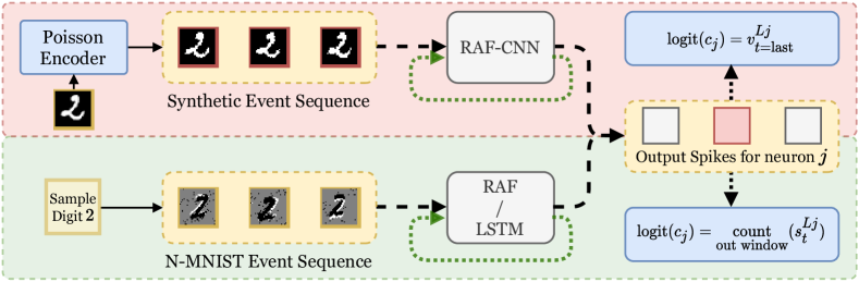
Figure 4: Above (red): Encoding and model pipeline for the RAF-CNN, trained on MNIST data. Below (green): Model pipeline for the N-MNIST-based experiments with RAF and LSTM networks.

We consider $4$ different models: RAF vs. LSTM, and RAF-CNN vs. CNN. A plain RAF network is analogous to a fully-connected (FC) network with one hidden layer but uses RAF neurons instead and is therefore recurrent. This is compared to an LSTM (Hochreiter & Schmidhuber, 1997) with a similar configuration. Table 1 shows the baseline architecture for each along with the number of trainable parameters. Note that the RAF model contains significantly fewer parameters than its counterpart yet outperforms it as discussed in Section 3.

Table 1: Comparing the RAF vs. LSTM models

RAF		LSTM
Layer Type	Dimension	Layer Type	Dimension
Input	34x34x2	Input	34x34x2
Flatten	2312	Flatten	2312
RAF	512	LSTM	512
Linear	10	Linear	10
# of Params	297,768	# of Params	1,251,594

Table 2 compares the RAF-CNN model with its non-spiking counterpart. They both follow LeNet architecture as in Lee et al. (2020). The RAF-CNN employs convolutional layers in place of FC layers in the RAF. The “Spiking Average Pooling” layer follows the same spatial-pooling method as in Lee et al. (2020) but uses the HardSoft activation function (Yanguas-Gil, 2020) instead as described in Section 2.3 with the $\beta$ and thresholds made learnable. The “Convolution” layer in the CNN uses a ReLU activation function. The RAF-CNN contains more trainable parameters because each neuron has a set of parameters: the damping factor ($\xi$), the natural frequency ($\omega$), the firing threshold ($\theta$), and the steepness of the sigmoid ($\beta$)—used to approximate the gradient in the backward pass.

Table 2: Comparing the RAF-CNN vs. CNN models

RAF-CNN				CNN
Layer Type	Kernel Size	Dimension	Stride	Layer Type	Kernel Size	Dimension	Stride
Input		28x28x1		Input		28x28x1
RAF Convolution	5x5	128	1	Convolution	5x5	128	1
Spiking Avg Pooling	2x2		2	Avg Pooling	2x2		2
RAF Convolution	5x5	128	1	Convolution	5x5	128	1
Spiking Avg Pooling	2x2		2	Avg Pooling	2x2		2
Flatten		6272		Flatten		6272
Spiking Linear		200		Linear + ReLU		200
Spiking Linear		10		Linear		10
# of Parameters	1,671,576			# of Parameters	1,669,200

References

- Ankit et al. (2017) Aayush Ankit, Abhronil Sengupta, Priyadarshini Panda, and Kaushik Roy. Resparc: A reconfigurable and energy-efficient architecture with memristive crossbars for deep spiking neural networks. In Proceedings of the 54th Annual Design Automation Conference 2017, pp. 1–6, 2017.
- Davies et al. (2018) Mike Davies, Narayan Srinivasa, Tsung-Han Lin, Gautham Chinya, Yongqiang Cao, Sri Harsha Choday, Georgios Dimou, Prasad Joshi, Nabil Imam, Shweta Jain, et al. Loihi: A neuromorphic manycore processor with on-chip learning. Ieee Micro, 38(1):82–99, 2018.
- Diehl et al. (2015) P. U. Diehl, D. Neil, J. Binas, M. Cook, S. Liu, and M. Pfeiffer. Fast-classifying, high-accuracy spiking deep networks through weight and threshold balancing. In 2015 International Joint Conference on Neural Networks (IJCNN), pp. 1–8, 2015. doi: 10.1109/IJCNN.2015.7280696.
- Fukushima (1980) Kunihiko Fukushima. Neocognitron: A self-organizing neural network model for a mechanism of pattern recognition unaffected by shift in position. Biological Cybernetics, 36:193–202, 1980.
- Hassabis et al. (2017) Demis Hassabis, Dharshan Kumaran, Christopher Summerfield, and Matthew M Botvinick. Neuroscience-inspired artificial intelligence. Neuron, 95:245–258, 2017.
- Hochreiter & Schmidhuber (1997) Sepp Hochreiter and Jürgen Schmidhuber. Long short-term memory. Neural Comput., 9(8):1735–1780, November 1997. ISSN 0899-7667. doi: 10.1162/neco.1997.9.8.1735. URL https://doi.org/10.1162/neco.1997.9.8.1735.
- Hubel & Wiesel (1968) D. H. Hubel and T. N. Wiesel. Receptive fields and functional architecture of monkey striate cortex. The Journal of Physiology, 195(1):215–243, 1968. doi: https://doi.org/10.1113/jphysiol.1968.sp008455. URL https://physoc.onlinelibrary.wiley.com/doi/abs/10.1113/jphysiol.1968.sp008455.
- Izhikevich (2001) E Izhikevich. Resonate-and-fire neurons. Neural Networks, pp. Vol 14, 883–894, 2001.
- LeCun et al. (1998) Yann LeCun, Léon Bottou, Yoshua Bengio, and Patrick Haffner. Gradient-based learning applied to document recognition. Proceedings of the IEEE, 86(11):2278–2324, 1998.
- Lee et al. (2020) Chankyu Lee, Syed Shakib Sarwar, Priyadarshini Panda, Gopalakrishnan Srinivasan, and Kaushik Roy. Enabling spike-based backpropagation for training deep neural network architectures. Frontiers in Neuroscience, 14:119, 2020. ISSN 1662-453X. doi: 10.3389/fnins.2020.00119. URL https://www.frontiersin.org/article/10.3389/fnins.2020.00119.
- Lee et al. (2016) Jun Haeng Lee, Tobi Delbruck, and Michael Pfeiffer. Training deep spiking neural networks using backpropagation. Frontiers in Neuroscience, 10:508, 2016. ISSN 1662-453X. doi: 10.3389/fnins.2016.00508. URL https://www.frontiersin.org/article/10.3389/fnins.2016.00508.
- Lichtsteiner et al. (2008) P. Lichtsteiner, C. Posch, and T. Delbruck. A 128 128 120 db 15 s latency asynchronous temporal contrast vision sensor. IEEE Journal of Solid-State Circuits, 43(2):566–576, 2008. doi: 10.1109/JSSC.2007.914337.
- Lindsay (2020) Grace W. Lindsay. Convolutional neural networks as a model of the visual system: Past, present, and future. Journal of Cognitive Neuroscience, pp. 1–15, Feb 2020. ISSN 1530-8898. doi: 10.1162/jocn˙a˙01544. URL http://dx.doi.org/10.1162/jocn_a_01544.
- Loshchilov & Hutter (2019) Ilya Loshchilov and Frank Hutter. Decoupled weight decay regularization. In International Conference on Learning Representations, 2019. URL https://openreview.net/forum?id=Bkg6RiCqY7.
- Merolla et al. (2014) Paul A. Merolla, John V. Arthur, Rodrigo Alvarez-Icaza, Andrew S. Cassidy, Jun Sawada, Filipp Akopyan, Bryan L. Jackson, Nabil Imam, Chen Guo, Yutaka Nakamura, Bernard Brezzo, Ivan Vo, Steven K. Esser, Rathinakumar Appuswamy, Brian Taba, Arnon Amir, Myron D. Flickner, William P. Risk, Rajit Manohar, and Dharmendra S. Modha. A million spiking-neuron integrated circuit with a scalable communication network and interface. Science, 345(6197):668–673, 2014. ISSN 0036-8075. doi: 10.1126/science.1254642. URL https://science.sciencemag.org/content/345/6197/668.
- O’Connor et al. (2013) Peter O’Connor, Daniel Neil, Shih-Chii Liu, Tobias Delbrück, and Michael Pfeiffer. Real-time classification and sensor fusion with a spiking deep belief network. Frontiers in Neuroscience, 7:178, 2013. ISSN 1662-453X. doi: 10.3929/ethz-b-000075617.
- Orchard et al. (2015) Garrick Orchard, Ajinkya Jayawant, Gregory K. Cohen, and Nitish Thakor. Converting static image datasets to spiking neuromorphic datasets using saccades. Frontiers in Neuroscience, 9:437, 2015. ISSN 1662-453X. doi: 10.3389/fnins.2015.00437. URL https://www.frontiersin.org/article/10.3389/fnins.2015.00437.
- Pauley et al. (2018) M Pauley, M Dutschmann, JH Manton, P Tolmachev, and RR Dhingra. Modeling the respiratory central pattern generator with resonate-and-fire izhikevich-neurons. Lecture Notes in Computer Science, pp. Vol 11301, 2018. doi: 10.1007/978-3-030-04167-0˙55. URL https://doi.org/10.1007/978-3-030-04167-0_55.
- Rescorla & Wagner (1972) RA Rescorla and Allan Wagner. A theory of Pavlovian conditioning: Variations in the effectiveness of reinforcement and nonreinforcement, volume Vol. 2. 01 1972.
- Rueckauer et al. (2017) Bodo Rueckauer, Iulia-Alexandra Lungu, Yuhuang Hu, Michael Pfeiffer, and Shih-Chii Liu. Conversion of continuous-valued deep networks to efficient event-driven networks for image classification. Frontiers in neuroscience, 11:682, 2017.
- Schultz et al. (1997) Wolfram Schultz, Peter Dayan, and P. Read Montague. A neural substrate of prediction and reward. Science, 275(5306):1593–1599, 1997. ISSN 0036-8075. doi: 10.1126/science.275.5306.1593. URL https://science.sciencemag.org/content/275/5306/1593.
- Sengupta et al. (2019) Abhronil Sengupta, Yuting Ye, Robert Wang, Chiao Liu, and Kaushik Roy. Going deeper in spiking neural networks: Vgg and residual architectures. Frontiers in neuroscience, 13:95, 2019.
- Torikai & Hishiki (2009) H Torikai and T Hishiki. Bifurcation analysis of a resonate-and-fire-type digital spiking neuron. Lecture Notes in Computer Science, pp. Vol 5864, 2009. doi: 10.1007/978-3-642-10684-2˙44. URL https://doi.org/10.1007/978-3-642-10684-2_44.
- Yanguas-Gil (2020) Angel Yanguas-Gil. Coarse scale representation of spiking neural networks: backpropagation through spikes and application to neuromorphic hardware. In International Conference on Neuromorphic Systems 2020, pp. 1–7, 2020.