Zero-energy Andreev bound states in iron-based superconductor Fe(Te,Se)

Abstract

Majorana bound states have been predicted to exist in vortices of topological superconductors (SC). A realization of the Fu-Kane model, based on a three-dimensional topological insulator brought into proximity to an $s$-wave SC, in iron-based SC Fe(Te,Se) has attracted strong interest after pronounced zero-energy bias peaks were observed in several experiments. Here, we show that, by taking into account inhomogeneities of the chemical potential or the presence of potential impurities on the surface of Fe(Te,Se), the emergence of these zero-energy bias peaks can be explained by trivial Andreev bound states (ABSs) whose energies are close to zero. Our numerical simulations reveal that the ABSs behave similarly to Majorana bound states. ABSs are localized only on the, say, top surface and cannot be distinguished from their topological counterparts in transport experiments performed with STM tips. Thus, such ABSs deserve a careful investigation of their own.

Introduction. Majorana bound states (MBSs) attracted substantial interest due to their promise to open a path to realize topologically protected operations for fault-tolerant quantum computing based on their non-Abelian braiding statistic [1, 2, 3, 4, 5, 6, 7, 8, 9, 10, 11, 12]. Since the first model of MBSs in one-dimensional (1D) $p$-wave superconductor (SC) was proposed by Kitaev [13, 14] many scenarios for generating MBSs have been put forward, e.g. in semiconductor nanowires with strong spin-orbit coupling and Zeeman field [15, 16, 17, 18, 19, 20, 21, 22, 23], in carbon-based materials [24, 25, 26, 27, 28, 29, 30], in magnetic atomic chains [31, 32, 33, 34, 35, 36, 37, 38, 39, 40], in topological insulator (TI) nanowires [41, 42, 43], in two-dimensional (2D) ferromagnetic insulator-semiconductor heterostructures [44, 45, 46, 47, 48, 49, 50, 51], and in three-dimensional (3D) strong TIs coupled to conventional $s$-wave SCs [52, 53, 54, 55, 56, 57]. Some of the above models have been reported to be realized experimentally [20, 21, 22, 23, 30, 38, 39, 40, 66, 67, 68, 69, 70, 71, 72, 73, 58, 59, 60, 61, 62, 63, 64, 65], enriching the ecosphere of Majorana physics.

Among the enumerated proposals, one of the most attractive options to be realized is the Fu-Kane model [52], which utilizes the helical property of the Dirac surface states in 3D TIs as an ideal platform for producing MBSs without the need of a Zeeman field or of fine-tuning the chemical potential inside the bulk gap. This model has been announced to be fully realized in a preexisting iron-based SC $\rm{FeTe}_{0.55}\rm{Se}_{0.45}$ by several experimental groups [74, 75, 76, 77, 78]. It was demonstrated that the key ingredients of Fe(Te,Se) for the advent of MBSs are the intrinsic superconducting phase, originally brought out from FeSe layered system, and the strong TI phase, induced by the band inversion along the $\Gamma-Z$-line in the Brillouin zone as a result of Te substitution [79]. Such an intrinsic topological superconductivity makes Fe(Te,Se) a highly promising material for Majorana-based topological quantum computing.

However, in spite of this progress, there are important issues to be clarified concerning this popular iron-based SC [80, 81]. Some groups have reported the low-ratio of the appearance of MBSs in the superconducting vortices of Fe(Te,Se) [77], and some reported their absence [81]. Even though a well shaped zero-bias peak (ZBP) as well as a half-integer shifted linear scaling relation of the surface modes can be observed [76], the coexisting non-topological regions mixed with zero-energy states in the vortices on the surface might also hamper the practicability of Fe(Te,Se). Actually, this complexity in experiments can be attributed to the intrinsic chemical inhomogeneity which comes from the nonuniform substitution of Se atoms, unavoidable defects, or excess iron atoms due to the special stoichiometry of Fe(Te,Se), as validated by scanning topography [82]. Regarding this “dirty” composition of Fe(Te,Se) SC, it is thus an urgent question to clarify whether the observed zero-energy states in Fe(Te,Se) are MBSs, which can be used as robust topological qubits, or whether this ZBP could be attributed to trivial Andreev bound states (ABSs) as was demonstrated in other MBS platforms [83, 84, 85, 86, 87, 88, 89, 90, 91, 92, 93, 94, 95, 96, 97, 98, 99, 100, 101].

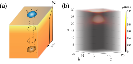
Figure 1: (a) The schematic diagram of 3D TI SC with a $z$-dependent electrostatic potential $U(z)$ shown by the solid curve. An external magnetic field induces a superconducting vortex (dashed lines), which hosts a set of low-energy states. (b) The local density of states (LDOS) distribution $\rho$ for the lowest-energy ABS inside the vortex. The non-uniform chemical potential confines the ABS close to the upper surface.

Here we aim to answer this question. We show that, by using a simple theoretical model of a 3D TI proximitized with an $s$-wave SC, the zero-energy states on the Fe(Te,Se) surface could be trivial ABSs arising as a result of the inhomogeneity in the chemical potential or, equivalently, in the electrostatic potential. Such inhomogeneity could find their origin in non-uniform gating of the sample, in the presence of impurities on the surface or in the bulk, as well as in band bending near the surface [see Fig. 1(a)]. All these inhomogeneities could be responsible for the appearance of zero-energy ABSs [see Fig. 1(b)]. Our numerical simulations identify regimes where a pair of MBSs located on opposite surfaces of Fe(Te,Se) is replaced by zero-energy quasi-MBSs or ABSs localized only on the, say, top surface. A further numerical simulation of scanning tunneling spectroscopy (STS) measurements on the surface spectrum with band bending gives qualitatively the same results as the experiments, which unveils the impossibility of experimentally distinguishing MBSs from trivial ABSs. Our results provide a new view of point on recent experiments in Fe(Te,Se) and could help to guide follow-up experiments uniquely identifying MBSs.

Model. We here adopt a 3D TI-SC lattice model [102, 103, 104, 105], which has been proven to capture basic properties of superconductivity in Fe(Te,Se). The Hamiltonian of the 3D TI [102] in momentum space can be written as: $\hat{H}=\int d{\bm{k}}\ \hat{c}^{\dagger}({\bm{k}})H_{0}({\bm{k}})\hat{c}({\bm{k}})$ with $\hat{c}({\bm{k}})=[\hat{c}_{1\uparrow}({\bm{k}}),\hat{c}_{1\downarrow}({\bm{k}}),\hat{c}_{2\uparrow}({\bm{k}}),\hat{c}_{2\downarrow}({\bm{k}})]^{T}$, where the vector consists of annihilation operators acting on electrons characterized by the orbital and spin degrees of freedom. Here, $H_{0}({\bm{k}})=\hbar v\sigma_{x}(s_{x}\sin{k_{x}a}+s_{y}\sin{k_{y}a}+s_{z}\sin{k_{z}a})+m({\bm{k}})\sigma_{z}$ with $m({\bm{k}})=m_{0}-m_{1}(\cos{k_{x}a}+\cos{k_{y}a})-m_{2}\cos{k_{z}a}$. The Pauli matrices $\sigma_{i}$ and $s_{i}$ act on orbital and spin space, respectively. In our lattice model we set $\hbar v=10\ {\rm meV}$ and $a=2.5\ {\rm nm}$ (the lattice constant of the cubic lattice to be used as the length unit).

We work with an isotropic $s$-wave superconducting pairing, which is sufficient to investigate the excitations within a single vortex line threading opposite surfaces in Fe(Te,Se) SC. The Bogoliubov-de-Gennes (BdG) Hamiltonian describing a uniform 3D TI-SC setup can be written as:

$$H_{\rm BdG}({\bm{k}})=\left(\begin{array}[]{cc}H_{0}({\bm{k}})-\mu_{0}&i\Delta_{0}s_{y}\\ -i\Delta_{0}s_{y}&\mu_{0}-H_{0}^{*}(-{\bm{k}})\end{array}\right)$$ (3)

in the basis $[\hat{c}({\bm{k}}),\hat{c}^{\dagger}(-{\bm{k}})]$. Here $\mu_{0}$ is the chemical potential and $\Delta_{0}$ represents the superconducting gap. By choosing the parameters: $m_{0}=-4$, $m_{1}=-2$, and $m_{2}=1$ (in units of $\hbar v$), $H_{0}({\bm{k}})$ describes a strong TI with helical surface states and a band gap $\Delta_{\rm TI}=10\ {\rm meV}$ at the band inversion point $Z$. To fit to the regime of experiments [74, 75, 76, 77, 78], we set the SC gap $\Delta_{0}=1.8\ {\rm meV}$.

It is predicted that, inside the vortex of the 3D TI-SC, a pair of MBSs appears at the ends of the vortex line [52]. Here, we consider a single vortex line induced by an external magnetic field. The superconducting pairing potential increases linearly with $r$ inside the vortex and is constant outside of the boundary $r_{0}$: $\Delta({\bm{r}})=\Delta_{0}[\Theta(r-r_{0})+\Theta(r_{0}-r)\cdot r/r_{0}]e^{i\theta}$. The coordinates in the cylindrical system are $(r,\theta)$, and $\Theta(r)$ is the step function. The orbital and Zeeman effects of the magnetic field can be neglected in our model due to the large London penetrating depth in Fe(Te,Se) SC [106]. By considering a finite-size system along the $z$ axis, our model well reproduces a pair of localized MBSs on the surfaces [see Supplementary Material (SM) [107]].

Non-uniform potential close to the surface and ABSs. In view of possible inhomogeneities in Fe(Te,Se), we use a position-dependent electrostatic potential $U(z)$. Although the chemical potential $\mu_{0}=5\ {\rm meV}$ on the surface is inside the TI gap, the inhomogeneity in the potential due to gating or the presence of impurities might result in the local chemical potential $\mu(z)\equiv\mu_{0}+U(z)$ (measured from the Dirac point of the TI) to cross conduction or valence bands. We note that the electrochemical potential stays constant and there is no current. For simplicity, we first consider a linear potential $U(z)=\kappa\hbar v(N_{z}-z)/(N_{z}-1)$, where $N_{z}$ is the height of the sample. The strength of the electric field is characterized by the parameter $\kappa$. Different types of $U(z)$ profile are considered in the SM [107]. We find that the obtained results do not depend on a particular shape of the potential. It is also not necessary to have the gradient over the entire sample. It is sufficient that $\mu$ is non-uniform on the surface.

In Fig. 2(a) we plot a set of profiles of $\mu(z)$ by varying the gradient $\kappa$. A vortex phase transition (VPT), where the line vortex changes from being a 1D topological SC to a normal SC [108, 109, 110], occurs if $\mu(z)$ reaches a critical value $\mu_{c}$ [see dashed line in Fig. 2(a)]. To calculate $\mu_{c}$ one may calculate the $\pi$-Berry-phase point by setting $k_{z}=\pi$ in our model [108, 107], or numerically find the gap closing point of the lowest energy bands by considering a periodic system along $z$-direction. The point at which $\mu(z)$ reaches $\mu_{c}$ determines the spatial position at which the VPT occurs and the bottom MBS resides. When the gradient $\kappa$ is small ($\kappa<0.5$), one can observe a well-localized MBS on the top and one at the bottom surface, respectively. As $\kappa$ is increased, the bottom of the sample is in the topologically trivial phase and one expects that the MBS on the bottom surface moves upward along with the boundary of VPT and gets closer with the top MBS until they start to overlap and merge into an ABS or, alternatively, into two quasi-MBSs.

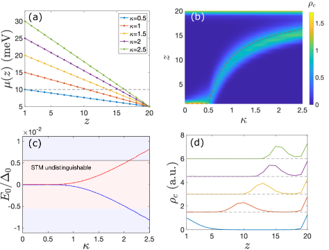
Figure 2: (a) A set of chemical potential profiles $\mu(z)$ (relative to the Dirac point of 3D TI) with different strength of electric field $\kappa$. The dashed line shows the critical chemical potential $\mu_{c}\approx 10\ {\rm meV}$ where the VPT happens. (b) The LDOS distribution $\rho_{c}$ along the center vortex line of the lowest energy state $E_{0}$ under varying $\kappa$. (c) The energy $E_{0}$ of the lowest bound state as a function of $\kappa$. For larger values of $\kappa$, two MBSs overlap and merge into a single ABS. In the STM undistinguishable energy range (pink color), one cannot distinguish between two types of bound states. (d) A set of LDOS curves with different $\kappa$, showing the crossover from MBSs to ABSs. Each curve is shifted with an equal distance of 1.5 (see the dashed grid). Here (a) and (d) share the same legend. The radius of the vortex is fixed to $r_{0}=5$. The system size is $N_{x}=N_{y}=31$, and $N_{z}=20$ and the surface chemical potential is $\mu_{0}=5\ {\rm meV}$.

A numerical calculation on the local density of states (LDOS) $\rho_{c}$ along the center of the vortex line confirms our expectations, as can be seen in Fig. 2(b). An estimated VPT boundary $z_{c}$ could be found by solving the equation $\mu_{0}+U(z_{c})=\mu_{c}$, also shown by a dashed line for comparison. A crossover from MBSs to ABSs occurs as $\kappa$ gets larger. The energy splitting is $E_{0}=0.76\ \mu{\rm eV}$ for the gradient $\kappa=1$. This corresponds to a weak electric field: $\epsilon=-\partial U(z)/\partial z\approx 0.21\ {\rm meV/nm}$ to be generated easily by some point defects or disorder [111, 112, 113]. In Fig. 2(d) we plot the profiles of the LDOS along the vortex line with different $\kappa$. As $\kappa>1$, the overlap of the wave functions becomes large, and these states can be identified as ABSs. Experimentally the resolution of the STM tip is about 20 $\mu{\rm eV}$ [77]. In Fig. 2(c) we label the energy range which cannot be distinguished by STM by pink color. Within this region, one cannot distinguish MBSs with ABSs. Only when $\kappa$ increases to about 2.1 can this energy splitting be measured with a manifestation of double peaks around zero in STS.

A point impurity on the surface. The surface of Fe(Te,Se) usually contains impurities or defects whose spatial dimensions are comparable to the size of the vortex [74, 75, 76, 77, 78], which may also influence the observation of the low-energy states. To include this effect, we consider a single impurity close to the top surface with $U_{\rm im}({\bf r})=-U_{0}e^{-R({\bf r})}$, where $R\equiv\sqrt{(x^{2}+y^{2})/\lambda^{2}_{\perp}+(z-z_{0})^{2}/\lambda^{2}_{z}}$ with $\lambda_{\perp}$ ($\lambda_{z}$) being the in-plane (out-of-plane) characteristic length scale, see Fig. 3(a). By changing $\lambda_{\perp}$ or $\lambda_{z}$, one can control the size of an area in which $\mu({\bf r})<\mu_{c}$. As a result, impurities close to the vortex center can generate nearly zero-energy ABSs, see Fig. 3. Even if the impurity potential is short-ranged, the ABS has almost zero energy. In this regime, it will be rather difficult to distinguish such local ABSs from MBSs localized both on the top and bottom TI surfaces. Generally, the smaller $\lambda_{z}$ is, the more localized is the zero-energy ABS next to the top surface, see Fig. 3(c). If one varies the width of the potential $\lambda_{\perp}$, the spatial positions of the ABSs along the $z$ axis stays unchanged [107], while their energy gets closer to zero for larger $\lambda_{\perp}$, mimicking MBSs.

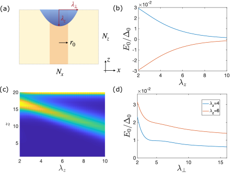
Figure 3: (a) The impurity potential $U_{\rm im}({\bf r})$ (blue) in the $xz$-plane of the 3D TI-SC. The lowest energy $E_{0}$ as a function of (b) $\lambda_{z}$ (for $\lambda_{\perp}=10$) and (d) $\lambda_{\perp}$. Even a short range potential of impurity creates a nearly zero-energy bound state, which could be confused with MBSs. (c) For small values of $\lambda_{z}$, the ABS is localized at the top surface, as can be seen in LDOS (for $\lambda_{\perp}=10$). Here we set $z_{0}=N_{z}$, $U_{0}=8{\rm meV}$, and the chemical potential far away from the impurity $\mu_{0}=13\ {\rm meV}$ corresponds to the trivial phase. Other parameters are the same with Fig. 2.

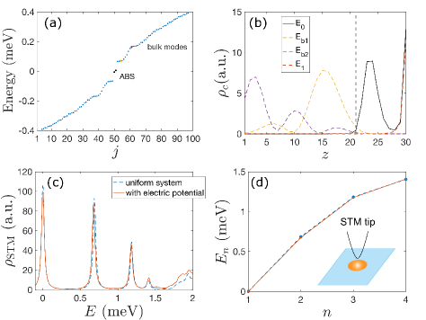
Figure 4: (a) The low-energy spectrum contains ABSs localized at the surface. An electrostatic potential is modeled by $U(z)=\kappa\hbar v[\Theta(21-z)+\Theta(z-21)(N_{z}-z)/(N_{z}-21)]$ with $\kappa=0.8$ and $N_{z}=30$. (b) The LDOS $\rho_{c}$ along the center vortex line for the ABSs localized at the top surface ($E_{0}=5.6\ \mu{\rm eV}$ and $E_{1}=0.676\ {\rm meV}$) and for the two bulk states ($E_{b1}=70\ {\mu}{\rm eV}$ and $E_{b2}=163{\mu}{\rm eV}$). The vertical dashed line denotes the boundary between the uniform and non-uniform regions at $z=21$. The 3D version of the ABS LDOS is also shown in Fig. 1. (c) The red (blue) line shows the results of the simulated LDOS $\rho_{\rm STM}$ of the STS measurement on the surface of Fe(Te,Se) for a system with a non-uniform (uniform) electrostatic potential hosting zero-energy ABSs (MBSs). The peaks are originating from ABSs with energy $E_{n}$ localized at the vortex. (d) The energies $E_{n}$ extracted from the LDOS curves are equidistantly distributed in both cases. The other parameters are the same as in Fig. 2.

Simulation of STM measurements on the surface of Fe(Te,Se) SC. Next, we study how trivial nearly zero-energy ABSs can be detected in STM experiments. To simulate realistic experimental samples we consider a thick layer with a non-uniform electrostatic potential. The lowest-energy ABS localized at the top surface inside the vortex is very close to zero energy ($E_{0}=5.6\ \mu{\rm eV}$), see Fig. 4(a). Its LDOS (3D LDOS) distribution along the vortex line is shown with black curve in Fig. 4(b) [in Fig. 1(b)]. The next ABS also localized on the surface ($E_{1}=0.676\ {\rm meV}$) is indicated by the red dashed line. Compared with clean systems (see Supplementary Material [107]), in addition to these ABSs localized next to the impurity, there are many low-energy bulk states localized in the vortex. In Fig. 4(b), for comparison, we also plot the LDOS distribution of two bulk states ($E_{b1}=70\ {\mu}{\rm eV}$ and $E_{b2}=163\ {\mu}{\rm eV}$) along the vortex line. We note that the ABSs and low-energy bulk states are well separated spatially. Although such bulk states can slightly leak into the region with non-uniform potential, they never reach the surface and, thus, cannot be detected by STS measurements at the surface.

Next, we calculate numerically the LDOS inside the vortex on the top surface to simulate STS measurements. The LDOS at energy $E$ is defined as [114]:

$$\rho_{\rm STM}(E)=-{\rm Im}\sum_{|{\bm{r}}_{i}-{\bm{r}}_{c}|<r_{0}}{\rm Tr}\,{G}^{r}({\bm{r}}_{i},E)/\pi,$$ (4)

where ${G}^{r}({\bm{r}_{i}},E)=[(E+i\eta)-{H}_{\rm BdG}]^{-1}$ is the retarded Green function. Here, ${\bm{r}}_{c}$ is the position of the vortex center and the summation in Eq. (4) is over the vortex region on the top surface. An imaginary term with $\eta=0.02\ {\rm meV}$ is included to account for the energy broadening in the STS measurement.

The localized ABSs are responsible for a series of well-sequenced LDOS peaks with a pronounced zero-energy peak, see Fig. 4(c) [solid curve]. As expected, the low-energy bulk states cannot be read out in the LDOS curve. To compare with signals coming from MBSs, we also show the LDOS curve for a case of uniform electrostatic potential in the topological phase (see the dashed curve). Only little difference can be seen between these two LDOS curves, indicating that normal measurements on the surface fail to distinguish ABSs with MBSs. In Fig. 4(d), we extract these ABS energy levels $E_{n}$ and plot them as a function of the level index $n$. It is different from the half-integer sequence $E_{n}\propto n+1/2$ of excitations in vortices of normal SC [115]. Instead, the relation $E_{n}\propto n$ is reproduced typical for topological vortices is reproduced, see Fig. 4(d). This result is in remarkable agreement with recent experimental observations interpreted as MBSs [76], but, here, it originates from trivial ABSs.

Discussion and conclusions. In conclusion, we have clarified the ambiguity of recent experimental observations on the zero-energy states in iron-based SC Fe(Te,Se), using a simple model of 3D TI proximity with an $s$-wave SC. We show that, if there are non-uniform electrostatic potentials near the surface of Fe(Te,Se) as a result of chemical inhomogeneity, presence of impurities, applied bias, these zero-energy states might well be ABSs instead of MBSs. Numerical simulations show that the ABSs have energies close to zero and are localized close to the top surface in contrast to MBSs assumed to be localized on both top and the bottom surfaces. These ABSs are thus incapable for topological quantum computing as they are easily destroyed by decoherence or impurity scattering. Still, these ABSs show other features usually associated with MBSs, unveiling the failure of STS measurements on distinguishing them. All these results imply that more careful studies are needed to ensure beyond reasonable doubt that Fe(Te,Se) SCs provide a robust platform for topological quantum computing.

Our results indicate again that it is far from sufficient to confirm MBSs by solely measuring the ZBP peaks. A rigorous characterization of the wavefunction, e.g. its localization, is also a necessary condition in searching for this exotic states. To make progress in this field, it seems indicated to go beyond static detection methods and instead use dynamic schemes, such as non-Abelian braiding operations on MBSs [17, 119], or other exotic properties in quantum transport concerned with them [120, 121, 122, 123, 124].

- [1] N. Read and D. Green, Phys. Rev. B 61, 10267 (2000).
- [2] C. W. J. Beenakker, Annu. Rev. Condens. Matter Phys. 4, 113-136 (2013).
- [3] M. Leijnse and K. Flensberg, Semicond. Sci. Technol. 27, 124003 (2012).
- [4] F. Wilczek, Nat. Phys. 5, 614-618 (2009).
- [5] X.-L. Qi and S.-C. Zhang, 83, 1057 (2011).
- [6] K. Laubscher and J. Klinovaja, arXiv:2104.14459;
- [7] D. A. Ivanov, Phys. Rev. Lett. 86, 268 (2001).
- [8] G. E. Volovik, The Universe in a Helium Droplet (Oxford Uni- versity Press, Oxford, 2003).
- [9] C. W. J. Beenakker, Annu. Rev. Condens. Matter Phys. 4, 113 (2013).
- [10] M. Sato and Y. Ando, Rep. Prog. Phys. 80, 076501 (2017).
- [11] R. R. Biswas, Phys. Rev. Lett. 111, 136401 (2013).
- [12] M. Cheng, R. M. Lutchyn, V. Galitski, and S. Das Sarma, Phys. Rev. Lett. 103, 107001 (2009).
- [13] A. Kitaev, Ann. Phys. (N.Y.) 303, 2 (2003).
- [14] E. Lieb, T. Schultz, and D. Mattis, Ann. Phys. 16, 407 (1961).
- [15] R. M. Lutchyn, J. D. Sau, and S. Das Sarma, Phys. Rev. Lett. 105, 077001 (2010).
- [16] Y. Oreg, G. Refael, and F. von Oppen, Phys. Rev. Lett. 105, 177002 (2010).
- [17] J. Alicea, Y. Oreg, G. Refael, F. von Oppen, and M. P. A. Fisher, Nat. Phys. 7, 412-417 (2011).
- [18] S. Tewari, T. D. Stanecu, J. D. Sau, and S. Das Sarma, New J. Phys. 13, 065004 (2011).
- [19] J. Klinovaja, P. Stano, and D. Loss, Phys. Rev. Lett. 109, 236801 (2012).
- [20] V. Mourik, K. Zuo, S. M. Frolov, S. R. Plissard, E. P. A. M. Bakkers, and L. P. Kouwenhoven, Science 336, 1003 (2012).
- [21] A. Das, Y. Ronen, Y. Most, Y. Oreg, M. Heiblum, and H. Shtrikman, Nat. Phys. 8, 887 (2012).
- [22] L. P. Rokhinson, X. Liu, and J. K. Furdyna, Nat. Phys. 8, 795 (2012).
- [23] M. T. Deng, C. L. Yu, G. Y. Huang, M. Larsson, P. Caroff, and H. Q. Xu, Nano Lett. 12, 6414 (2012).
- [24] J. Klinovaja, S. Gangadharaiah, and D. Loss, Phys. Rev. Lett. 108, 196804 (2012).
- [25] R. Egger and K. Flensberg, Phys. Rev. B 85, 235462 (2012).
- [26] J. Klinovaja and D. Loss, Phys. Rev. X 3, 011008 (2013).
- [27] J. D. Sau and S. Tewari, Phys. Rev. B 88, 054503 (2013).
- [28] C. Dutreix, M. Guigou, D. Chevallier, and C. Bena, Eur. Phys. J. B 87, 296 (2014).
- [29] M. Marganska, L. Milz, W. Izumida, C. Strunk, and M. Grifoni, Phys. Rev. B 97, 075141 (2018).
- [30] M. M. Desjardins, L. C. Contamin, M. R. Delbecq, M. C. Dartiailh, L. E. Bruhat, T. Cubaynes, J. J. Viennot, F. Mallet, S. Rohart, A. Thiaville, A. Cottet, and T. Kontos, Nat. Mater. 18, 1060 (2019).
- [31] S. Nadj-Perge, I. K. Drozdov, B. A. Bernevig, and A. Yazdani, Phys. Rev. B 88, 020407(R) (2013).
- [32] J. Klinovaja, P. Stano, A. Yazdani, and D. Loss, Phys. Rev. Lett. 111, 186805 (2013).
- [33] B. Braunecker and P. Simon, Phys. Rev. Lett. 111, 147202 (2013).
- [34] M. M. Vazifeh and M. Franz, Phys. Rev. Lett. 111, 206802 (2013).
- [35] T.-P. Choy, J. M. Edge, A. R. Akhmerov, and C. W. J. Beenakker, Phys. Rev. B 84, 195442 (2011).
- [36] F. Pientka, L. I. Glazman, and F. von Oppen, Phys. Rev. B 88, 155420 (2013).
- [37] B. Jäck, Y. Xie, and A. Yazdani, arXiv:2103.13210.
- [38] S. Nadj-Perge, I. K. Drozdov, J. Li, H. Chen, I. K. Jeon, J. Seo, A. H. MacDonald, B. A. Bernevig, and A. Yazdani, Science 346, 602 (2014).
- [39] M. Ruby, F. Pientka, Y. Peng, F. von Oppen, B. W. Heinrich, and K. J. Franke, Phys. Rev. Lett. 115, 197204 (2015).
- [40] R. Pawlak, M. Kisiel, J. Klinovaja, T. Meier, S. Kawai, T. Glatzel, D. Loss, and E. Meyer, npj Quantum Inf. 2, 16035 (2016).
- [41] A. Cook and M. Franz, Phys. Rev. B 84, 201105(R) (2011).
- [42] A. M. Cook, M. M. Vazifeh, and M. Franz, Phys. Rev. B 86, 155431 (2012).
- [43] H. F. Legg, D. Loss, and J. Klinovaja, arXiv:2103.13412.
- [44] J. D. Sau, R. M. Lutchyn, S. Tewari, and S. Das Sarma, Phys. Rev. Lett. 104, 040502 (2010).
- [45] J. D. Sau, S. Tewari, R. M. Lutchyn, T. D. Stanescu, and S. Das Sarma, Phys. Rev. B 82, 214509 (2010).
- [46] X.-L. Qi, T. L. Hughes, and S.-C. Zhang, Phys. Rev. B 82, 184516 (2010).
- [47] N. Sedlmayr, V. Kaladzhyan, C. Dutreix, and C. Bena, Phys. Rev. B 96, 184516 (2017).
- [48] A. C. Potter and P. A. Lee, Phys. Rev. B 83, 184520 (2011).
- [49] M. Sato, Y. Takahashi, and S. Fujimoto, Phys. Rev. Lett. 103, 020401 (2009).
- [50] M. Sato, Y. Takahashi, and S. Fujimoto, Phys. Rev. B 82, 134521 (2010);
- [51] M. Sato and S. Fujimoto, J. Phys. Soc. Jpn. 85, 072001 (2016).
- [52] L. Fu and C. L. Kane, Phys. Rev. Lett. 100, 096407 (2008).
- [53] L. Fu and C. L. Kane, Phys. Rev. Lett. 102, 216403 (2009).
- [54] A. R. Akhmerov, J. Nilsson, and C. W. J. Beenakker, Phys. Rev. Lett. 102, 216404 (2009).
- [55] J. Linder, Y. Tanaka, T. Yokoyama, A. Sudbø, and N. Nagaosa, Phys. Rev. Lett. 104, 067001 (2010).
- [56] Y. Tanaka, T. Yokoyama, and N. Nagaosa, Phys. Rev. Lett. 103, 107002 (2009).
- [57] K. T. Law, P. A. Lee, and T. K. Ng, Phys. Rev. Lett. 103, 237001 (2009).
- [58] S.-Y. Xu et al., Nat. Phys. 10, 943-950 (2014).
- [59] J.-P. Xu et al., Phys. Rev. Lett. 112, 217001 (2014).
- [60] J.-X. Yin et al., Nat. Phys. 11, 543-546 (2015).
- [61] C. Chen, K. Jiang, Y. Zhang, C. Liu, Y. Liu, Z. Wang and J. Wang, Nat. Phys. 16, 536-540 (2020).
- [62] B. Jäck, Y. Xie, J. Li, S. Jeon, B. Andrei Bernevig, and A. Yazdani, Science 364, 1255-1259 (2019).
- [63] G. C. Ménard et al., Nat. Commun. 8, 2040 (2017).
- [64] H. Kim et al., Sci. Adv. 4, eaar5251 (2018).
- [65] S. Manna, P. Wei, Y. Xie, K. T. Law, P. A. Lee and J. S. Moodera, Proc. Natl. Acad. Sci. 117, 8775–8782 (2020).
- [66] M. T. Deng, S. Vaitiekenas, E. B. Hansen, J. Danon, M. Leijnse, K. Flensberg, J. Nygård, P. Krogstrup and C. M. Marcus, Science 354, 1557-1562 (2016).
- [67] L. P. Rokhinson, X. Liu, and J. K. Furdyna, Nat. Phys. 8, 795-799 (2012).
- [68] J.P. Xu et al., Phys. Rev. Lett. 114, 017001 (2015).
- [69] H.-H. Sun, K.-W. Zhang, L.-H. Hu, C. Li, G.-Y. Wang, H.-Y. Ma et al., Phys. Rev. Lett. 116, 257003 (2016).
- [70] J. R. Williams et al., Phys. Rev. Lett. 109, 056803 (2012).
- [71] S. Sasaki, M. Kriener, K. Segawa, K. Yada, Y. Tanaka, M. Sato, and Y. Ando, Phys. Rev. Lett. 107, 217001 (2011).
- [72] S. Nadj-Perge, I. K. Drozdov, J. Li, H. Chen, S. Jeon, J. Seo, A. H. MacDonald, B. A. Bernevig, and A. Yazdani, Science 346, 602-607 (2014).
- [73] S. Jeon, Y. Xie, J. Li, Z. Wang, B. Andrei Bernevig, and A. Yazdani, Science 358, 772-776 (2017).
- [74] D. Wang et al., Science 362, 333-335 (2018).
- [75] P. Zhang, K. Yaji, T. Hashimoto, Y. Ota, T. Kondo, K. Okazaki, Z. Wang, J. Wen, G. D. Gu, H. Ding, and S. Shin, Science 360, 182-186 (2018).
- [76] L. Kong et al., Nat. Phys. 15, 1181-1187 (2019).
- [77] T. Machida, Y. Sun, S. Pyon, S. Takeda, Y. Kohsaka, T. Hanaguri, T. Sasagawa, and T. Tamegai, Nat. Mater. 18, 811-815 (2019).
- [78] S. Zhu et al., Science 367, 189-192 (2020).
- [79] Z. Wang et al., Phys. Rev. B 92, 115119 (2015).
- [80] W. Liu et al., Nat. Commun. 11, 5688 (2020).
- [81] M. Chen, X. Chen, H. Yang, Z. Du, X. Zhu, E. Wang, and H.-H. Wen, Nat. Commun. 9, 970 (2018).
- [82] X. He, G. Li, J. Zhang, A. B. Karki, R. Jin, B. C. Sales, A. S. Sefat, M. A. McGuire, D. Mandrus, and E. W. Plummer, Phys. Rev. B 83, 220502(R) (2011).
- [83] E. Prada, P. San-Jose, M. W. A. de Moor, A. Geresdi, E. J. H. Lee, J. Klinovaja, D. Loss, J. Nygard, R. Aguado, and L. P. Kouwenhoven, Nat. Rev. Phys. 2, 575 (2020).
- [84] G. Kells, D. Meidan, and P. W. Brouwer, Phys. Rev. B 86, 100503(R) (2012).
- [85] C. Fleckenstein, F. Dominguez, N. Traverso Ziani, and B. Trauzettel, Phys. Rev. B 97, 155425 (2018).
- [86] F. Penaranda, R. Aguado, P. San-Jose, and E. Prada, Phys. Rev. B 98, 235406 (2018).
- [87] A. Ptok, A. Kobialka, and T. Domanski, Phys. Rev. B 96, 195430 (2017).
- [88] C. Moore, T. D. Stanescu, and S. Tewari, Phys. Rev. B 97, 165302 (2018).
- [89] C.-X. Liu, J. D. Sau, T. D. Stanescu, and S. Das Sarma, Phys. Rev. B 96, 075161 (2017).
- [90] D. J. Alspaugh, D. E. Sheehy, M. O. Goerbig, and P. Simon, Phys. Rev. Research 2, 023146 (2020).
- [91] C. Reeg, O. Dmytruk, D. Chevallier, D. Loss, and J. Klinovaja, Phys. Rev. B 98, 245407 (2018).
- [92] B. D. Woods, J. Chen, S. M. Frolov, and T. D. Stanescu, Phys. Rev. B 100, 125407 (2019).
- [93] C.-X. Liu, J. D. Sau, T. D. Stanescu, and S. Das Sarma, Phys. Rev. B 99, 024510 (2019).
- [94] J. Chen, B. D.Woods, P. Yu, M. Hocevar, D. Car, S. R. Plissard, E. P. A. M. Bakkers, T. D. Stanescu, and S. M. Frolov, Phys. Rev. Lett. 123, 107703 (2019).
- [95] E. J. H. Lee, X. Jiang, R. Aguado, G. Katsaros, C. M. Lieber, and S. De Franceschi, Phys. Rev. Lett. 109, 186802 (2012).
- [96] C. Junger, R. Delagrange, D. Chevallier, S. Lehmann, K. A. Dick, C. Thelander, J. Klinovaja, D. Loss, A. Baumgartner, and C. Schonenberger, Phys. Rev. Lett. 125, 017701 (2020).
- [97] O. Dmytruk, D. Loss, and J. Klinovaja, Phys. Rev. B 102, 245431 (2020).
- [98] P. Yu, J. Chen, M. Gomanko, G. Badawy, E. P. A. M. Bakkers, K. Zuo, V. Mourik, and S. M. Frolov, arXiv:2004.08583.
- [99] M. Kayyalha, D. Xiao, R. Zhang, J. Shin, J. Jiang, F. Wang, Y.-F. Zhao, R. Xiao, L. Zhang, K. M. Fijalkowski, P. Mandal, M. Winnerlein, C. Gould, Q. Li, L. W. Molenkamp, M. H. W. Chan, N. Samarth, and C.-Z. Chang, Science 367, 64 (2020).
- [100] M. Valentini, F. Penaranda, A. Hofmann, M. Brauns, R. Hauschild, P. Krogstrup, P. San-Jose, E. Prada, R. Aguado, and G. Katsaros, arXiv:2008.02348.
- [101] H. Kim, Y. Nagai, L. Rózsa, D. Schreyer, and R. Wiesendanger, arXiv: 2105.01354.
- [102] R.-X. Zhang, W. S. Cole, and S. Das Sarma, 122, 187001 (2019).
- [103] A. Ghazaryan, P. L. S. Lopes, P. Hosur, M. J. Gilbert, and P. Ghaemi, Phys. Rev. B 101, 020504(R) (2020).
- [104] C.-K. Chiu, T. Machida, Y. Huang, t. Hanaguri, and F.-C. Zhang, Sci. Adv. 6, eaay0443 (2020).
- [105] S. Qin, L. Hu, X. Wu, X. Dai, C. Fang, F.-C. Zhang, and J. Hu, Science Bulletin 64, 1207-1214 (2019).
- [106] H. Kim et al., Phys. Rev. B 81, 180503(R) (2010).
- [107] See Supplementary Material for the discussion on the finite-size effect, the calculation on the critical chemical potential , the calculation with hyperbolic surface potential, and the discussion on the point impurity.
- [108] P. Hosur, P. Ghaemi, R. S. K. Mong, and A. Vishwanath, Phys. Rev. Lett. 107, 097001 (2011).
- [109] C.-K. Chiu, P. Ghaemi, and T. L. Hughes, Phys. Rev. Lett. 109, 237009 (2012).
- [110] Sayed Ali Akbar Ghorashi, T. L. Hughes, and E. Rossi, Phys. Rev. Lett. 125, 037001 (2020).
- [111] Z. Hou, Y.-F. Zhou, X. C. Xie, and Q.-F. Sun, Phys. Rev. B 99, 125422 (2019).
- [112] F. Ghahari et al., Science 356, 845 (2017).
- [113] Y. Zhao, J. Wyrick, F. D. Natterer, J. F. Rodriguez-Nieva, C. Lewandowski, K. Watanabe, T. Taniguchi, L. S. Levitov, N. B. Zhitenev, and J. A. Stroscio, Science 348, 672 (2015).
- [114] Z. Hou, and Q.-F. Sun, Phys. Rev. Res. 2, 023236 (2020).
- [115] G. E. Volovik, JETP Lett. 70, 609-614 (1999).
- [116] S. Tewari, S. Das Sarma, and Dung-Hai Lee, Phys. Rev. Lett. 99, 037001 (2007).
- [117] H. Pan, and S. Das Sarma, arXiv:2102.07296 (2021).
- [118] H. Pan, and S. Das Sarma, Phys. Rev. Res. 2, 013377 (2020).
- [119] C. W. J. Beenakker, SciPost Phys. Lect. Notes 15 (2020).
- [120] L. Fu, and C. L. Kane, Phys. Rev. B 79, 161408(R) (2009).
- [121] S. Das Sarma, C. Nayak, and S. Tewari, Phys. Rev. B 73, 220502(R) (2006).
- [122] E. Grosfeld, B. Seradjeh, and S. Vishveshwara, Phys. Rev. B 83, 104513 (2011).
- [123] G. Strübi, W. Belzig, M.-S. Choi, and C. Bruder, Phys. Rev. Lett. 107, 136403 (2011).
- [124] Y.-T. Zhang, Z. Hou, X. C. Xie, and Q.-F. Sun, Phys. Rev. B 95, 245433 (2017).