Fast-Slow Transformer for Visually Grounding Speech

Abstract

We present Fast-Slow Transformer for Visually Grounding Speech, or FaST-VGS. FaST-VGS is a Transformer-based model for learning the associations between raw speech waveforms and visual images. The model unifies dual-encoder and cross-attention architectures into a single model, reaping the superior retrieval speed of the former along with the accuracy of the latter. FaST-VGS achieves state-of-the-art speech-image retrieval accuracy on benchmark datasets, and its learned representations exhibit strong performance on the ZeroSpeech 2021 phonetic and semantic tasks.

Index Terms—  visually-grounded speech, vision and language, self-supervised speech processing

1 Introduction and Related Work

Humans acquire spoken language long before they can read and write. They do so in a multimodal fashion, by learning to relate the speech patterns they hear with sensory percepts occurring in other modalities, such as vision. Recently, a number of works on learning from visually-grounded speech have addressed the question of whether machines can acquire knowledge of spoken language in a similar fashion [1]. Researchers have investigated the benefits of incorporating visual context into automatic speech recognition [2, 3], as a pre-training task for supervised ASR [4], word detection and localization [5, 6, 7, 8], hierarchical linguistic unit analysis [9, 10], cross-modality alignment [11, 12, 13], speech segmentation [14], speech generation [15], multilingual spoken language learning [16, 17, 18, 19].

Many of these works have used retrieval between images and their spoken audio captions as a training task to learn speech representations from visual supervision. Although retrieval accuracy was often used as an evaluation benchmark to assess how well a model can predict visual semantics directly from a raw speech signal, in many cases these papers put a greater emphasis on analyzing how linguistic structure emerged within the representations learned by the model. In general, the accuracy of speech-image retrieval systems has lagged behind their text-image counterparts, but recently several works have made enormous progress towards closing this gap, demonstrating that speech-enabled image retrieval is a compelling application in its own right [20, 21, 22, 23].

In this work, we propose Fast-Slow Transformer for Visually Grounding Speech, or FaST-VGS, the first Transformer [24]-based model for speech-image retrieval. FaST-VGS uses a novel coarse-to-fine training and retrieval method, which unifies the dual-encoder and cross-attention architectures, enabling both fast and accurate retrieval using a single model. FaST-VGS achieves state-of-the-art speech-image retrieval accuracy on the Places Audio [25], the Flickr8k Audio Caption Corpus (FACC) [26], and SpokenCOCO [15] benchmark corpora. In addition, we study the linguistic information encoded in the speech representations learned by FaST-VGS by evaluating it on the phonetic and semantic tasks of the ZeroSpeech 2021 Challenge [27] Visually-Grounded Track [28].

2 Technical Approach

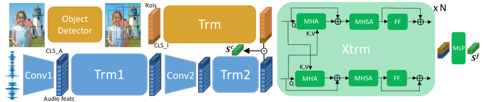
Fig. 1: Architecture of the FaST-VGS model.

The FaST-VGS model is designed to take as input a visual image $I$ and an acoustic speech waveform $A$ that describes the contents of $I$, and output a similarity score that is large when $A$ faithfully describes the content of $I$, and small otherwise. Crucially, we design the model to output two different similarity scores. The coarse similarity $S^{c}$ is simply the dot product between independently embedded vector representations of $I$ and $A$, enabling computationally fast retrieval at the cost of reduced accuracy. Alternatively, the model can output a fine similarity $S^{f}$ that leverages cross-modal self-attention to jointly encode $I$ and $A$, leading to more accurate but slower retrieval. Our model (Fig. 1) is composed of three modules: an audio encoder, an image encoder, and a cross-modal encoder, which we discuss in detail.

The audio encoder takes as input the raw waveform of $A$, represented as a 1-D vector of sample amplitudes. It passes this waveform through a convolutional block (Conv1) to obtain features at a high temporal resolution. Then, these features are augmented with a CLS_A token and input to a Transformer stack (Trm1) for contextualization. The contextualized high resolution features (with the exception of the CLS_A token) are then fed into a second convolutional network (Conv2) in order to reduce their temporal resolution. This is done to better capture higher level semantic information carried over a longer time span (e.g. by words and phrases), as well as to make the subsequent application of cross-modal attention less computationally expensive. The output of the Conv2 network is concatenated back with the CLS_A token, and then fed as input to a second Transformer stack (Trm2) to perform another round of contextualization. At this point, the CLS_A output of the Trm2 block can be directly used to compute the coarse similarity $S^{c}$, or all of the outputs can be carried onwards into the cross-modal Transformer block in order to compute the fine similarity $S^{f}$. The image encoder contains two components. First, an object detector extracts a set of regions of interest (RoI) accompanied by their features and positions. Then, similar to the audio branch, a CLS_I token is concatenated with RoI and position features which are input to a Transformer stack (Trm). At this point, the output CLS_I token from the Trm block can be used with the CLS_A token to compute the coarse score $S^{c}$, or fed with the contextualized RoI features into the cross-modal transformer to compute the fine score $S^{f}$. Finally, the cross-modal encoder (Xtrm) takes as input the outputs of the Trm and Trm2 blocks and passes them through a series of cross-modal Transformer blocks that perform contextualization over both input modalities at once. For the Xtrm module, we use a slightly modified version of the Cross-Modality Encoder introduced by [29], in which each block is composed of a multi-head cross-attention mechanism, followed by a multi-head self attention mechanism and finally two feedforward layers. Residual connections are added around the cross-attention and feedforward layers. Differently from [29], our cross-modal encoder outputs only the CLS_A and CLS_I tokens, which are then concatenated and passed to a three-layer MLP to produce a scalar representing $S^{f}$.

To perform retrieval, we compute similarity scores between an input query (image or spoken description) and all of the items in the held-out target dataset, and return the $K$ items with the largest scores. Fine scores are more expensive to compute than the coarse scores, since the query must be paired with each target item and passed through the cross-modal attention module. In contrast, the embeddings of the target items used to compute the coarse scores may be pre-computed and re-used for each query. However, we expect the coarse scores to offer worse performance than the fine scores since they cannot leverage cross-modal attention. We can simultaneously achieve high speed and accuracy by using coarse-to-fine retrieval (CTF). CTF retrieval uses a two-pass strategy, where coarse retrieval is first used to retrieve a set of $K_{c}$ target items, where $K_{c}$ is set to be significantly larger than the $K$ items we ultimately want the model to return, but much smaller than the full size of the target dataset. The coarse feature outputs of the $K_{c}$ target items along with the coarse features of the query are then passed to the cross-modal encoder to produce fine similarity scores, which are used for final ranking and the return of the top $K$ target items. Our experiments in Sec. 3 confirm that CTF can reduce retrieval time by as much as 98% compared to fine retrieval, while maintaining nearly the same accuracy.  [30] recently proposed a similar idea for text-to-image retrieval, where a cross-modal transformer teacher model was used to train a dual encoder student model. Our work differs from theirs in that we use a unified model for both coarse and fine retrieval, which is trained end-to-end with a simple objective.

For training, we follow [22] and use the masked margin softmax loss that is simultaneously applied in both possible directions of retrieval within a batch. Given a batch of $B$ pairs of images and audio captions we first compute the similarity score $S^{*}_{i,j}$ between the $i^{th}$ audio caption and the $j^{th}$ image, where $S^{*}$ can be either the coarse matching score $S^{c}$ or the fine matching score $S^{f}$. For a given matching score type, the loss is then defined as: $\mathcal{L}^{*}=\mathcal{L}^{*}_{A\rightarrow{I}}+\mathcal{L}^{*}_{I\rightarrow{A}},$ where

$$\mathcal{L}^{*}_{A\rightarrow{I}}=-\frac{1}{B}\sum_{i=1}^{B}\log\frac{e^{S^{*}_{i,i}-\delta}}{e^{S^{*}_{i,i}-\delta}+\sum_{j=1}^{B}M_{i,j}e^{S^{*}_{i,j}}}$$ (1)

$$\mathcal{L}^{*}_{I\rightarrow{A}}=-\frac{1}{B}\sum_{i=1}^{B}\log\frac{e^{S^{*}_{i,i}-\delta}}{e^{S^{*}_{i,i}-\delta}+\sum_{j=1}^{B}M_{j,i}e^{S^{*}_{j,i}}}$$ (2)

We assume that when $i=j$ the audio caption and image are matched, but both FACC and SpokenCOCO contain multiple audio captions for each image. In this case, it is possible that within a batch, certain images will have a ground-truth match with multiple audio captions. To prevent these from being treated as negative examples by the loss function, we use masking variables $M_{i,j}$ which are $0$ when audio caption $i$ matches image $j$, and 1 otherwise. We train the model to optimize both the coarse and fine matching losses simultaneously using the overall loss $\mathcal{L}=\lambda^{c}\mathcal{L}^{c}+\lambda^{f}\mathcal{L}^{f}$.

3 Experiments

Datasets. We train and test our models on the Places Audio [25], SpokenCOCO [15], and Flickr8k Audio Captions [26] (FACC) datasets. Places Audio contains 400k images from the the MIT Places 205 [31] dataset and each image has a single corresponding audio caption that was recorded spontaneously by a human as they viewed the image. Both SpokenCOCO and FACC were produced by having humans speak aloud the text captions accompanying the MSCOCO [32] and Flickr8k [33] datasets, respectively. SpokenCOCO contains 123k images, each with 5 spoken captions, while FACC contains 8k images each with 5 spoken captions. We use the standard train/dev/test splits for FACC, the Karpathy splits [34] for SpokenCOCO, and the “2020” splits for Places Audio. Finally, we use the publicly-distributed development set of the ZeroSpeech 2021 Challenge [27, 28] to evaluate the phonetic and semantic information learned by our model.

Table 1: Performance of FaST-VGS on the Places Audio, averaged between the 2020 “dev-seen” and “dev-unseen” splits as well as between $A\rightarrow I$ and $I\rightarrow A$ retrieval.

Method	Time/Query	$\lambda^{c}$	$\lambda^{f}$	R@1	R@5	R@10
		1	0	56.9	85.2	91.4
		1	1	60.7	87.3	93.0
		1	0.1	57.0	85.3	91.7
Coarse	6.1ms	0.1	1	61.8	87.7	93.3
		0	1	66.8	89.1	93.7
		1	1	63.0	88.3	93.4
		1	0.1	56.5	84.7	91.7
Fine	83.3ms	0.1	1	67.8	90.5	94.7
		1	1	63.4	88.3	93.5
		1	0.1	56.7	84.9	91.5
CTF	12.2ms	0.1	1	67.8	90.5	94.6

Implementation details. For the audio branch, we use the convolutional encoder and first 8 layers of the Transformer stack from wav2vec2.0 [35] as the Conv1 and Trm1 blocks in our model. We initialize the weights of both blocks with the pretrained “Base” model, and we freeze the Conv1 weights during training. We found that using only the first 8 wav2vec2.0 transformer layers performs better than using all 12 layers. Conv2 uses the ResDAVEnet architecture [11] with the dimension of first convolutional layer changed to match Trm1’s hidden dimension. Trm2 is a one layer standard Transformer, and both Conv2 and Trm2 are randomly initialized. For the image encoder, we use the off-the-shelf Faster-RCNN [36] . We freeze Faster-RCNN weights, and extract the top 36 RoIs for each image. The RoI features are fed to a 6-layer Transformer (Trm), which is randomly initialized. The cross-modal encoder consists of two blocks, (N=2 in Figure 1). All Transformer layers in our model use a hidden dimension of 768 and 8 attention heads (except for Trm1, which uses 12 attention heads). The 3-layer MLP that computes $S^{f}$ has layers of width 1536, 768, and 1, and uses GELU [37] activations. To select $(\lambda^{c},\lambda^{f})$ we do a grid search over $\{0,0.1,1\}\times\{0,0.1,1\}$ on the Places Audio development set. All models are trained using BertAdam [38] with a linear warm-up over the first $10\%$ of training steps, a peak learning rate $1e-4$, and a linear decay to 0 over the course of training. For all experiments, we set $\delta=1$ and $K_{c}=100$. Models on Places and SpokenCOCO are trained for $20$ epochs with batch size $48$ and $64$, both taking less than $3$ days on $8$ NVIDIA V100 GPUs. Models on FACC are trained for $60$ epochs with batch size $96$, and this takes about $0.5$ days on $8$ V100 GPUs.

Table 2: Comparison of FaST-VGS with other models on the Places Audio Captions. Subscript CO means coarse retrieval.

	Places Audio (test-seen)						Places Audio (test-unseen)
	Speech $\rightarrow$ Image			Image $\rightarrow$ Speech			Speech $\rightarrow$ Image			Image $\rightarrow$ Speech
Model	R@1	R@5	R@10	R@1	R@5	R@10	R@1	R@5	R@10	R@1	R@5	R@10
ResDAVEnet [4]	35.2	67.5	78.0	30.4	63.1	74.1	38.3	68.5	78.8	31.2	65.0	75.4
MILAN [23]	58.4	84.6	90.6	53.8	83.4	90.1	62.1	86.0	90.5	58.2	85.8	90.9
$\text{FaST-VGS}_{\text{CO}}$	60.0	86.1	92.3	60.2	85.1	92.2	62.8	88.4	92.9	62.3	89.0	93.2
$\text{FaST-VGS}_{\text{CTF}}$	64.0	88.3	93.7	64.2	87.9	92.2	69.6	90.3	94.3	66.0	90.4	94.1

Table 1 displays the retrieval accuracy and time per query using coarse, fine, and CTF retrieval methods on the Places Audio dev set when varying the weights on the coarse and fine loss terms. For all three retrieval methods, $(\lambda^{c},\lambda^{f})=(0.1,1)$ achieves the highest scores. This indicates that even when coarse or fine matching are used alone, training the model with both losses is beneficial. Additionally, putting more weight on the fine matching loss is important regardless of the retrieval method used. In light of this, we fix $(\lambda^{c},\lambda^{f})=(0.1,1)$ for the remainder of our experiments. We also notice that CTF maintains the accuracy of fine retrieval, while being nearly as fast as coarse retrieval. The speed gap is exacerbated when using a larger target database: on SpokenCOCO (which contains 5k images and 25k captions in the evaluation set), fine and CTF retrieval achieve the same R@10 scores of $83.0$, but their average retrieval times per query are $399.7$ ms and $8.4$ ms. In Table. 2, we compare the retrieval accuracy of FaST-VGS on the Places Audio test sets with other models from the literature and show that both retrieval methods significantly outperform MILAN [23] which is the previous state-of-the-art for this task. We also note that the MILAN model was pretrained on 3.3 million image and spoken caption pairs from the Conceptual Spoken Captions (CSC) [22] dataset, and hypothesize that training FaST-VGS on a large dataset would widen the performance gap further.

In Table. 3, we present retrieval results on FACC and SpokenCOCO. When trained only on FACC, FaST-VGS outperforms all previously published models trained on the same dataset, but still underperforms the MILAN model pretrained on CSC. To probe whether this is due to the disparity in training data amounts, we pretrain a FaST-VGS model on SpokenCOCO and fine-tune it on FACC. This model significantly outperforms MILAN, despite the fact that the CSC dataset (3.3 million images and captions) is far larger than SpokenCOCO (123k images and 615k spoken captions). At the bottom of Table 3 we present retrieval results on SpokenCOCO. The MILAN model preceded the SpokenCOCO dataset and hence did not report results on it, but we compare to the ResDAVEnet [11] baseline model. We also compare to DIME [39], a current state-of-the-art model for image-text matching on MSCOCO, which can be considered an oracle upperbound for our model as DIME has access to the ground truth text being spoken. FaST-VGS significantly outperforms ResDAVEnet, and performs respectably against DIME in terms of average R@10 score (82.45 vs 86.25). To test the performance of DIME on ASR text, we use the code and model weights open sourced by the authors and transcribe the SpokenCOCO test set using the Google ASR API. We denote this model as $\text{DIME}_{\text{ASR}}$ in Table. 3. The gap between FaST-VGS and $\text{DIME}_{\text{ASR}}$ is much smaller than DIME, and our $\text{FaST-VGS}_{\text{CTF}}$ performs equally or better in two of the six metrics compared to $\text{DIME}_{\text{ASR}}$.

Table 3: Results on FACC and SpokenCOCO. ${\dagger}$ indicates a model trained with text supervision. * indicates a model trained on SpokenCOCO and FACC.

	Speech $\rightarrow$ Image			Image $\rightarrow$ Speech
Model	R@1	R@5	R@10	R@1	R@5	R@10
	Flickr8k (test 1k)
[9]	5.5	16.3	25.3	-	-	-
[18]	9.6	-	-	-	-	-
[20]†	-	-	29.6	-	-	-
[6]	12.7	34.9	48.5	16.0	42.8	56.1
[40]†	21.8	49.9	63.1	-	-	-
$\text{FaST-VGS}_{\text{CO}}$	26.6	56.4	68.8	36.2	66.1	76.5
$\text{FaST-VGS}_{\text{CTF}}$	29.3	58.6	71.0	37.9	68.5	79.9
[22]	13.9	36.8	49.5	18.2	43.5	55.8
MILAN [23]	33.2	62.7	73.9	49.6	79.2	87.5
$\text{FaST-VGS}^{*}_{\text{CO}}$	41.2	70.4	81.5	53.6	81.1	89.5
$\text{FaST-VGS}^{*}_{\text{CTF}}$	45.5	73.8	83.7	59.8	84.1	90.7
	SpokenCOCO (test 5k)
ResDAVEnet [4]	17.3	41.9	55.0	22.0	50.6	65.2
$\text{FaST-VGS}_{\text{CO}}$	31.8	62.5	75.0	42.5	73.7	84.9
$\text{FaST-VGS}_{\text{CTF}}$	35.9	66.3	77.9	48.8	78.2	87.0
	Text $\rightarrow$ Image			Image $\rightarrow$ Text
DIME [39]	40.2	70.7	81.4	56.1	83.2	91.1
$\text{DIME}_{\text{ASR}}$	37.6	66.3	76.9	54.8	82.4	90.4

Table 4: Performance on the ZeroSpeech 2021 tasks. Both VG models (bottom) are trained on SpokenCOCO, while the non-VG models (top) are trained on Librispeech [41].

	Semantic $\uparrow$		ABX $\downarrow$
Model	Syn.	Lib.	W-C	W-O	A-C	A-O
[42]	4.29	7.69	0.03	0.05	0.04	0.08
[43]	5.90	10.20	0.03	0.04	0.04	0.07
VG Baseline (h.b.)	9.60	15.09	0.06	0.07	0.07	0.11
FaST-VGS	15.80	23.55	0.05	0.06	0.05	0.09

Finally, we investigate the speech representations learned by FaST-VGS by evaluating it on the phonetic and semantic tasks of the ZeroSpeech 2021 Challenge dev set. We use representations from layer $6$ of Trm1 and layer $1$ of Trm2 (max pooled) for phonetic and semantic tasks respectively, which we found to outperform the other layers in the model. In Tab. 4, we see that FaST-VGS achieves very high semantic scores for both sythesized speech and speech from Librispeech. For the phonetic ABX task, FaST-VGS outperforms the high budget VG baseline [28] in all four ABX evaluations, but underperforms best non-VG models.

4 Concluding Discussion

We presented FaST-VGS, a Transformer-based model for visually-grounded speech-image retrieval that achieves state-of-the-art results across 3 benchmark datasets, and makes use of a novel coarse-to-fine training and retrieval strategy that unifies the dual-encoder and cross-attention architectures into a single model. We analyzed the model’s learned representations on two of the ZeroSpeech 2021 tasks, confirming that they are strongly predictive of phonetic identity and lexical semantics. In our future work, we plan to investigate other linguistic information learned by the model, as well as ways of using the model’s self-attention heads for word and sub-word unit discovery.

References

- [1] G. Chrupała, “Visually grounded models of spoken language: A survey of datasets, architectures and evaluation techniques,” arXiv, 2021.
- [2] F. Sun, D. Harwath, and J. Glass, “Look, listen, and decode: Multimodal speech recognition with images,” in SLT, 2016.
- [3] S. Palaskar, R. Sanabria, and F. Metze, “End-to-end multimodal speech recognition,” in ICASSP, 2018.
- [4] W.-N. Hsu, D. F. Harwath, and J. Glass, “Transfer learning from audio-visual grounding to speech recognition,” in INTERSPEECH, 2019.
- [5] H. Kamper, S. Settle, G. Shakhnarovich, and K. Livescu, “Visually grounded learning of keyword prediction from untranscribed speech,” in INTERSPEECH, 2017.
- [6] D. Merkx, S. Frank, and M. Ernestus, “Language learning using speech to image retrieval,” in INTERSPEECH, 2019.
- [7] L. Wang and M. Hasegawa-Johnson, “A dnn-hmm-dnn hybrid model for discovering word-like units from spoken captions and image regions,” in INTERSPEECH, 2020.
- [8] K. Olaleye and H. Kamper, “Attention-based keyword localisation in speech using visual grounding,” in INTERSPEECH, 2021.
- [9] G. Chrupała, L. Gelderloos, and A. Alishahi, “Representations of language in a model of visually grounded speech signal,” in ACL, 2017.
- [10] D. F. Harwath, W.-N. Hsu, and J. R. Glass, “Learning hierarchical discrete linguistic units from visually-grounded speech,” in ICLR, 2020.
- [11] D. F. Harwath, A. Recasens, D. Surís, G. Chuang, A. Torralba, and J. Glass, “Jointly discovering visual objects and spoken words from raw sensory input,” IJCV, 2019.
- [12] L. Wang, X. Wang, M. Hasegawa-Johnson, O. Scharenborg, and N. Dehak, “Align or attend? toward more efficient and accurate spoken word discovery using speech-to-image retrieval,” in ICASSP, 2021.
- [13] K. Khorrami and O. Räsänen, “Evaluation of audio-visual alignments in visually grounded speech models,” in INTERSPEECH, 2021.
- [14] D. F. Harwath and J. R. Glass, “Towards visually grounded sub-word speech unit discovery,” in ICASSP, 2019.
- [15] W.-N. Hsu, D. F. Harwath, C. Song, and J. Glass, “Text-free image-to-speech synthesis using learned segmental units,” in ACL, 2021.
- [16] D. F. Harwath, G. Chuang, and J. R. Glass, “Vision as an interlingua: Learning multilingual semantic embeddings of untranscribed speech,” ICASSP, 2018.
- [17] H. Kamper and M. Roth, “Visually grounded cross-lingual keyword spotting in speech,” SLTU, 2018.
- [18] W. N. Havard, J.-P. Chevrot, and L. Besacier, “Catplayinginthesnow: Impact of prior segmentation on a model of visually grounded speech,” in CoNLL, 2020.
- [19] Y. Ohishi, A. Kimura, T. Kawanishi, K. Kashino, D. F. Harwath, and J. Glass, “Trilingual semantic embeddings of visually grounded speech with self-attention mechanisms,” ICASSP, 2020.
- [20] G. Chrupała, “Symbolic inductive bias for visually grounded learning of spoken language,” in ACL, 2019.
- [21] M. Mortazavi, “Speech-image semantic alignment does not depend on any prior classification tasks,” in INTERSPEECH, 2020.
- [22] G. Ilharco, Y. Zhang, and J. Baldridge, “Large-scale representation learning from visually grounded untranscribed speech,” in CoNLL, 2019.
- [23] R. Sanabria, A. Waters, and J. Baldridge, “Talk, don’t write: A study of direct speech-based image retrieval,” in INTERSPEECH, 2021.
- [24] A. Vaswani, N. M. Shazeer, N. Parmar, J. Uszkoreit, L. Jones, A. N. Gomez, L. Kaiser, and I. Polosukhin, “Attention is all you need,” in NeurIPS, 2017.
- [25] D. F. Harwath, A. Torralba, and J. R. Glass, “Unsupervised learning of spoken language with visual context,” in NIPS, 2016.
- [26] D. F. Harwath and J. R. Glass, “Deep multimodal semantic embeddings for speech and images,” ASRU, 2015.
- [27] T. A. Nguyen, M. de Seyssel, P. Rozé, M. Rivière, E. Kharitonov, A. Baevski, E. Dunbar, and E. Dupoux, “The zero resource speech benchmark 2021: Metrics and baselines for unsupervised spoken language modeling,” SAS @ NeurIPS, 2020.
- [28] A. Alishahi et al., “Zr-2021vg: Zero-resource speech challenge, visually-grounded language modelling track, 2021 edition,” 2021.
- [29] H. Tan and M. Bansal, “Lxmert: Learning cross-modality encoder representations from transformers,” in EMNLP, 2019.
- [30] A. Miech, J.-B. Alayrac, I. Laptev, J. Sivic, and A. Zisserman, “Thinking fast and slow: Efficient text-to-visual retrieval with transformers,” in CVPR, 2021.
- [31] B. Zhou, À. Lapedriza, J. Xiao, A. Torralba, and A. Oliva, “Learning deep features for scene recognition using places database,” in NeurIPS, 2014.
- [32] T.-Y. Lin, M. Maire, S. J. Belongie, J. Hays, P. Perona, D. Ramanan, P. Dollár, and C. L. Zitnick, “Microsoft coco: Common objects in context,” in ECCV, 2014.
- [33] M. Hodosh, P. Young, and J. Hockenmaier, “Framing image description as a ranking task: Data, models and evaluation metrics (extended abstract),” JAIR, 2013.
- [34] A. Karpathy and L. Fei-Fei, “Deep visual-semantic alignments for generating image descriptions,” TPAMI, 2017.
- [35] A. Baevski, H. Zhou, A. Mohamed, and M. Auli, “wav2vec 2.0: A framework for self-supervised learning of speech representations,” in NeurIPS, 2020.
- [36] S. Ren, K. He, R. B. Girshick, and J. Sun, “Faster r-cnn: Towards real-time object detection with region proposal networks,” TPAMI, 2015.
- [37] D. Hendrycks and K. Gimpel, “Gaussian error linear units (gelus),” ArXiv, 2016.
- [38] J. Devlin, M.-W. Chang, K. Lee, and K. Toutanova, “Bert: Pre-training of deep bidirectional transformers for language understanding,” in NAACL, 2019.
- [39] L. Qu, M. Liu, J. Wu, Z. Gao, and L. Nie, “Dynamic modality interaction modeling for image-text retrieval,” in ACM SIGIR, 2021.
- [40] B. Higy, D. Eliott, and G. Chrupała, “Textual supervision for visually grounded spoken language understanding,” in Findings of EMNLP, 2020.
- [41] V. Panayotov, G. Chen, D. Povey, and S. Khudanpur, “Librispeech: An asr corpus based on public domain audio books,” in ICASSP, 2015.
- [42] B. v. Niekerk, L. Nortje, M. Baas, and H. Kamper, “Analyzing speaker information in self-supervised models to improve zero-resource speech processing,” in INTERSPEECH, 2021.
- [43] J. Chorowski et al., “Information retrieval for zerospeech 2021: The submission by university of wroclaw,” ArXiv, 2021.