A Cautionary Tale of Decorrelating
Theory Uncertainties

Abstract

A variety of techniques have been proposed to train machine learning classifiers that are independent of a given feature. While this can be an essential technique for enabling background estimation, it may also be useful for reducing uncertainties. We carefully examine theory uncertainties, which typically do not have a statistical origin. We will provide explicit examples of two-point (fragmentation modeling) and continuous (higher-order corrections) uncertainties where decorrelating significantly reduces the apparent uncertainty while the actual uncertainty is much larger. These results suggest that caution should be taken when using decorrelation for these types of uncertainties as long as we do not have a complete decomposition into statistically meaningful components.

1 Introduction

Modern machine learning classifiers hold great promise for increasing the sensitivity of high energy physics data analyses Larkoski:2017jix ; Guest:2018yhq ; Albertsson:2018maf ; Radovic:2018dip ; Carleo:2019ptp ; Bourilkov:2019yoi ; Schwartz:2021ftp ; Feickert:2021ajf . Typically, a classifier is trained using simulations and then the number of events passing a fixed threshold on the classifier in data and in simulation is counted. A comparison between these counts is then used to estimate model parameters such as masses, couplings, and (new physics) cross sections (limits). Theoretical and experimental uncertainties on the final result are accounted for by varying an aspect of the simulation and recomputing the predicted count using the nominal classifier. The uncertainties in the model used for training affect the optimally of the classifier itself Nachman:2019dol , but typically do not cause a bias and can be accounted for Ghosh:2021roe by using parameterized classifiers Cranmer:2015bka ; Baldi:2016fzo .

A variety of techniques have been proposed to render a classifier independent of a given feature Louppe:2016ylz ; Dolen:2016kst ; Moult:2017okx ; Stevens:2013dya ; Shimmin:2017mfk ; Bradshaw:2019ipy ; ATL-PHYS-PUB-2018-014 ; DiscoFever ; Xia:2018kgd ; Englert:2018cfo ; Wunsch:2019qbo ; Rogozhnikov:2014zea ; 10.1088/2632-2153/ab9023 ; clavijo2020adversarial ; Kasieczka:2020pil ; Kitouni:2020xgb . This has become an essential tool for resonance searches, where thresholds on the classifier must not sculpt bumps in a given spectrum so that the Standard Model background can be estimated using sideband fits. The same methodology has also been proposed to reduce systematic uncertainties. If a classifier does not depend on a particular nuisance parameter, then the count computed when the parameter is varied will be the same as the nominal value. This means that the uncertainty on the parameter(s) of interest will appear to be reduced.

In the case that the systematic uncertainty is decomposed into its most fundamental components, each with a clear statistical interpretation, the above would be the end of the story. The systematic uncertainty can be reduced through decorrelation and this would be useful if the classification performance does not rely strongly on the value of the nuisance parameters (otherwise, it may be better to profile instead Ghosh:2021roe ). However, theory uncertainties almost never satisfy these conditions. These uncertainties are the result of approximations when performing calculations and are also due to parameter freedom in phenomenological models that are needed when first-principles calculations are not possible. The canonical examples for these two types of uncertainties are perturbative uncertainties from series truncation and fragmentation modeling. For the former, calculations are truncated at a fixed order in perturbation theory and the result depends on unphysical scales. These scales are varied typically by factors of two in order to determine the uncertainty. Fragmentation modeling uncertainties are often evaluated by comparing two different models, such as the string model Andersson:1983ia ; Sjostrand:1984ic in the Pythia Sjostrand:2006za ; Sjostrand:2007gs parton shower Monte Carlo (PSMC) and the cluster model Webber:1983if ; Winter:2003tt in the Herwig Bellm:2015jjp ; Bahr:2008pv PSMC. These variations are then interpreted as a one standard deviation uncertainty and combined with other sources of uncertainty in a final statistical analysis.

We examine the interplay of decorrelation with theory uncertainties. In particular, we will show that constructing a classifier that is independent of a given theory nuisance parameter does not mean that the theory uncertainty is zero. Instead, it means that the only handle to determine the theory uncertainty is eliminated. Figure 1 illustrates the intuition behind why this might be the case. As concrete examples, we study fragmentation modeling for Lorentz-boosted $W$ boson jet classification and factorization scale variations when classifying events as either from $W$+jets or $t$-channel single top quark events.

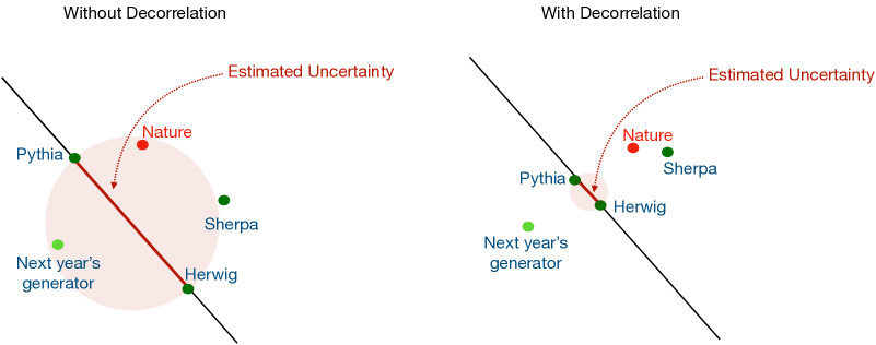
Figure 1: An illustration of the potential impact of training a classifier to be decorrelated to two-point uncertainties. The distance between Pythia and Herwig is treated as the uncertainty. Left: Without decorrelation, the uncertainty covers nature even if nature does not lie on the line connecting Pythia and Herwig. Right: The distance between Pythia and Herwig is reduced due to the decorrelation requirement, resulting in a smaller estimate of the uncertainty, which no longer covers nature. These diagrams are meant only to be intuitive illustrations.

This paper is organized as follows. Section 2 briefly introduces existing decorrelation techniques. Numerical examples of both two-point and continuous uncertainties are provided in Sec. 3. The paper ends with conclusions and outlook in Sec. 4.

2 Decorrelation Techniques

Let $x\in\mathbb{R}^{n}$ be the features used for classification. Suppose that there is a feature $m\in\mathbb{R}$ that we want to be decorrelated from a classifier $f(x):\mathbb{R}^{n}\rightarrow\mathbb{R}$. One can achieve this decorrelation by minimizing the following loss functional $L$:

$$L[f(x)]=\sum_{i\in S}L_{\text{class}}(f(x_{i}),1)+\sum_{i\in B}w(m_{i})L_{\text{class}}(f(x_{i}),0)+\lambda\,\sum_{i\in B}L_{\text{decor}}(f(x_{i}),m_{i})\,,$$ (1)

where $S$ and $B$ represent signal and background events, respectively. The loss $L_{\text{class}}$ is the classifier loss and is often the binary cross entropy $L_{\text{class}}(f(x),y)=y\log(f(x))+(1-y)\log(1-f(x))$. The function $w(m)$ represents a weighting function and $\lambda$ represents a hyperparameter that controls the strength of the decorrelation. Finally, $L_{\text{decor}}$ is a term that penalizes any dependence between $f$ and $m$. This last term in Eq. 1 is schematic as the decorrelation penalty often acts at the level of batches of events and not individual examples. Standard classification corresponds to $w(m)=1$ and $\lambda=0$. Decorrelation approaches include:

• Planing Chang:2017kvc ; 1511.05190 : $\lambda=0$ and $w(m_{i})\approx p_{S}(m)/p_{B}(m)$ so that the marginal distribution of $m$ is non-discriminatory after the reweighting.

• Adversaries Louppe:2016ylz ; Shimmin:2017mfk ; Englert:2018cfo ; clavijo2020adversarial : $w(m)=1$, $\lambda<0$, and $L_{\text{decor}}$ is the loss of a second neural network (adversary) that takes $f(x)$ as input and tries to learn some properties of $m$.

• Distance Correlation (DisCo) DiscoFever ; Kasieczka:2020pil : $w(m)=1,\lambda>0$, and the last term in Eq. (1) is the distance correlation szekely2007 ; szekely2009 ; SzeKely:2013:DCT:2486206.2486394 ; szekely2014 between $f(x)$ and $m$ for the background.

• Flatness Rogozhnikov:2014zea : $w(m)=1$, $\lambda>0$, and $L_{\text{decor}}=\sum_{m}b_{m}\int|F_{m}(s)-F(s)|^{2}\,{\rm d}s$ where the sum runs over mass bins, $b_{m}$ is the fraction of candidates in bin $m$, $F$ is the cumulative distribution function, and $s=f(x)$ is the classifier output. This is generalized to Moment Decorrelation (MoDE) in Ref. Kitouni:2020xgb to allow for a given dependence of $f$ on $m$.

In the examples below, we focus on the adversarial case as it is the most explored in the literature. However, the same ideas apply to all decorrelation methods.

3 Numerical Examples

All neural networks are implemented using Keras keras with the Tensorflow backend tensorflow and optimized with Adam adam .

3.1 Two-point Uncertainty: Fragmentation Modeling

General purpose event generators use perturbation theory when they can and phenomological models to describe non-perturbative effects such as hadronization. The standard procedure for estimating the uncertainty due to the model choice is to compare the predictions from two different models. This uncertainty is typical largest when the analysis strategy exploits subtle correlations in the high-dimensional radiation pattern. For example, tagging the origin of high $p_{T}$ jets is a widely-studied scenario ATLAS:2018wis ; CMS:2020poo ; Kasieczka:2019dbj for machine learning whereby the detailed jet substructure can be used for classification. In this section, we study Lorenz-boosted $W$ boson tagging, where the signal is hadronically decaying, high $p_{T}$ $W$ bosons and the background is generic quark and gluon jets. A single large-radius jet is often sufficient to capture most of the $W$ boson decay products and its two-prong substructure is distinct from typical quark and gluon jets.

Samples were generated with MadGraph5_aMC@NLO 2.7.3 (Alwall:2014hca, ) for modeling $pp$ collisions at $\sqrt{s}$ = 13 TeV. The NNPDF23_nlo_as_0118 (Ball:2012cx, ) parton distribution function is used. The hard-scattering events are passed to Pythia 8.303 (Sjostrand:2007gs, ) to simulate the parton shower and hadronization, using the default settings. Herwig 7.2.2 (Bellm:2015jjp, ) with angularly-ordered showers and Sherpa 2.2.2 (Gleisberg:2008ta, ; Sherpa:2019gpd, ) with default settings are also used to model the parton shower and hadronization. The jets are clustered by Pyjet (noel_dawe_2021_4446849, ; Cacciari:2011ma, ) and the anti-$k_{t}$ (Cacciari:2008gp, ) algorithm with radius parameter $R$ = 1.2.

A set of high-level jet substructure features are used to distinguish $W$ jets from QCD jets. These features are illustrated in Fig. 2 and briefly described in the following. The kinematics are probed with the jet mass and transverse momentum. Jet substructure observables include $n$-subjettiness ratio $\tau_{21}=\tau_{2}/\tau_{1}$ Thaler:2010tr ; Thaler:2011gf , and energy correlation function ratios $D_{2}^{(\beta)}=e_{3}^{(\beta)}/(e_{2}^{(\beta)})^{3}$ Larkoski:2014gra and $C_{2}^{(\beta)}=e_{3}^{(\beta)}/(e_{2}^{(\beta)})^{2}$ Larkoski:2013eya , where $e_{i}$ is the normalized sum over doublets ($i=2$) or triplets ($i=3$) of constituents inside jets, weighted by the product of the constituent transverse momenta and pairwise angular distances. For this analysis, we consider both $\beta=1$ and $\beta=2$.

As expected, the mass peaks near the $W$ boson mass of 80 GeV 10.1093/ptep/ptaa104 for the signal and has a broad distribution for the background. The signal peak is slightly higher than the $W$ boson mass due to underlying event and other event contamination. This could be mitigated with grooming Butterworth:2008iy ; Ellis:2009me ; Krohn:2009th ; Dasgupta:2013ihk ; Larkoski:2014wba . The jet $p_{T}$ is not very discriminating by construction. The two-prong nature of the signal jets is quantified by a low $\tau_{21},D_{2}$, and $C_{2}$.

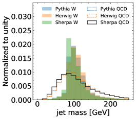
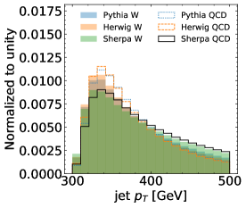
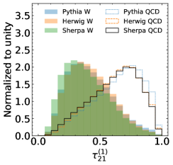
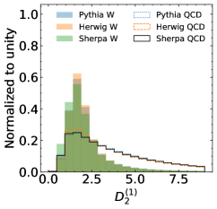
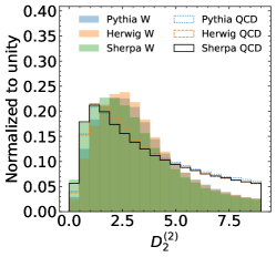
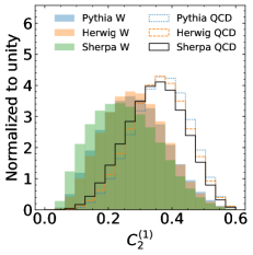
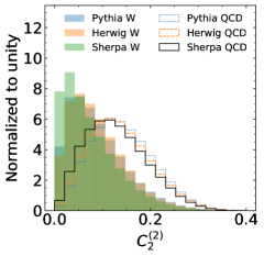
Figure 2: The seven inputs used to train a classifier to distinguish boosted $W$ boson jets from generic QCD jets events.

A classifier is trained using the seven features presented in Fig. 2 to distinguish $W$ jets from QCD jets. The nominal classifier is trained using the Pythia simulation and is parameterized as a neural network with two hidden layers of 50 nodes each. Rectified Linear Unit (ReLU) activations are used for the intermediate layers and the final output is passed through a sigmoid function. The binary cross-entropy is used for training with a batch size of 100 and for 20 epochs. None of these parameters were optimized, although minor variations were found to have little impact on performance. The performance of this nominal classifier evaluated on Pythia, Herwig, and Sherpa is shown in Fig. 3. We focus on the region near 10-15% signal efficiency, which is a typical working point for LHC analyses. In this range, the background rejection (inverse QCD efficiency) is between a few hundred and a few thousand.

A second network is trained as part of an adversarial approach. This second network uses both Pythia and Herwig events and minimizes the following loss:

$$L[f,g]= -\left(\sum_{i\in W}\log(f(x_{i}))-\sum_{i\in\text{QCD}}\log(1-f(x_{i}))\right)$$

$$+\lambda\left(\sum_{i\in\text{Pythia}}\log(g(f(x_{i}),y_{i}))-\sum_{i\in\text{Herwig}}\log(1-g(f(x_{i}),y_{i}))\right)\,,$$ (2)

where $y_{i}=0$ for $W$ jets and $y_{i}=1$ for QCD jets. Furthermore, $\lambda=10$. Note that unlike Eq. 1, Eq. 3.1 has the labels as part of the function for the adversary. This means that the labels for the classifier are given as an input feature to the adversary, which allows the adversary to potentially learn separate decision functions for $W$ jets and QCD jets. The classifier network $f$ has the same composition as the nominal classifier described above: two hidden layers with 50 nodes each. The adversary has five hidden layers with 50 nodes each. As $W$ jets are more different from QCD jets than Pythia jets are from Herwig jets, the adversary has a more difficult task, which is why $g$ has a more complex architecture. It was found that adding the label $y_{i}$ to $g$ as well as multiplying the gradient for the adversary by 10 improved performance and stability. The minimax nature of the optimization in Eq. 3.1 is implemented by connecting the adversary to the classifier via a gradient reversal layer pmlr-v37-ganin15 that multiplies the gradient by a fixed negative constant during backpropagation. The classifier network is then extracted after training for 20 epochs. When $\lambda=0$, the performance was found to be the same as for the nominal case.

Figure 3 shows that the performance of the adversarially trained classifier is worse than the nominal case. This drop in performance is the cost for building a classifier that is insensitive to fragmentation model variations. The difference between Pythia and Herwig for the nominal classifier is about 40% at 10% $W$ efficiency while it is only about 20% for the adversarially trained network. The reduced difference may give the impression that the adversarially trained classifier has successfully learnt to be less sensitive to fragmentation model variations. However, the difference between Sherpa and Pythia is nearly the same for the nominal and the adversarially trained classifier. This means that the ‘true’ uncertainty would be significantly underestimated if only Pythia and Herwig were available. It is often the case that only two fragmentation models are available.

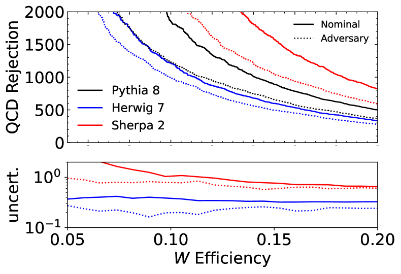
Figure 3: The QCD rejection (inverse QCD efficiency) as a function of the $W$ jet efficiency for classifiers applied to Pythia, Herwig, and Sherpa jets. The solid lines correspond to the nominal classifier trained with Pythia while the dotted lines correspond to the adversarial setup that uses both Pythia and Herwig. The bottom panel shows the relative absolute difference with respect to Pythia (nominal or adversarial, as appropriate). Note that the lower panel has a logarithmic vertical axis. While adversarial training reduces the difference in performance between Pythia and Herwig, the difference to Sherpa remains large, indicating that the the true uncertainty will be underestimated if a third independent sample is unavailable.

3.2 Continuous Uncertainty: Higher-order Corrections

The uncertainty from truncating the order of a perturbative calculation is typically estimated by varying the unphysical scales. Usually, there are renormalization scale and factorization scale uncertainties. For simplicity, we focus here on the factorization scale, which dictates the separation between long- and short-distance physics. The standard procedure is to set the factorization scale to the typical momentum transfer in the problem.

To study the impact of factorization scale variations, we consider measurements of $t$-channel single top quark production. One of the main backgrounds for this process is $W$+jets production and machine learning is already used by ATLAS ATLAS:2016qhd and CMS CMS:2019jjp to enhance the signal. The semileptonic channel is studied as it has a much smaller background than the all-hadronic channel. The final state is characterized by an isolated lepton, missing transverse momentum, and jets.

Events are simulated using MadGraph5_aMC@NLO (MG5_aMC) 3.1.1 Alwall:2014hca interfaced with Pythia 8.244 Sjostrand:2007gs for the parton shower and Delphes 3.4.2 deFavereau:2013fsa ; Mertens:2015kba ; Selvaggi:2014mya for detector simulations with the default CMS card. Particle flow candidates are used as inputs to jet clustering, implemented using FastJet 3.2.1 Cacciari:2011ma ; Cacciari:2005hq and the anti-$k_{t}$ algorithm Cacciari:2008gp with radius parameter $R=0.5$. For simplicity, $W$ bosons are forced to decay into muons and events are required to have at least one isolated and identified muon using the default reconstruction algorithm in Delphes. Usually, one uses the highest precision method possible and then scale variations give the uncertainty from the finite truncation of the perturbative series. In order to compare with the ‘true’ uncertainty, we artificially truncate the series early and then use the higher-order calculation as the reference uncertainty. In particular, the nominal simulation is performed at leading order (LO) in the strong coupling constant and then an additional sample for the $t$-channel process is simulated at next-to-leading order (NLO).

For the machine learning, events are represented by 12 numbers: the three-momentum of the muon, the four-momentum of the leading two jets, and the scalar sum of the transverse momenta of all jets ($H_{T}$). Momenta are specified by $p_{T}$, $\eta$, and $\phi$. Histograms for each of the observables for single top $t$-channel and $W$+jets are shown in Fig. 4. The jet $p_{T}$ spectra are harder for single top compared with $W$ jets and the muons (jets) tend to be more central (forward) for single top compared with $W$+jets.

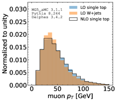
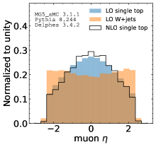
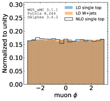
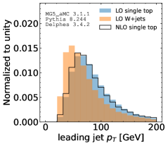
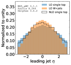
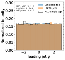
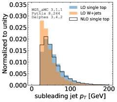
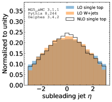
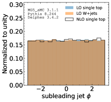
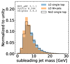
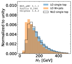
Figure 4: The 12 inputs used to train a classifier to distinguish single top events from $W$+jets events.

The impact of factorization scale variations is shown in Fig. 5. All variations are normalized to unity, as the impact on the total cross section is not relevant for per-event classification performance. As expected, the variation for all $\phi$ observables is negligible and the biggest variation occurs for the transverse momenta.

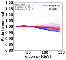
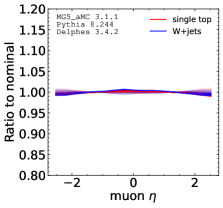
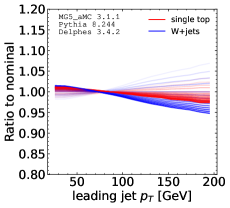
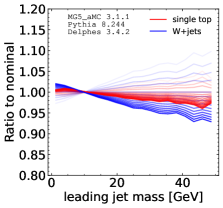
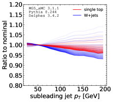
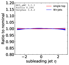
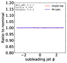
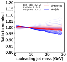
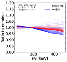
Figure 5: The impact of factorization scale variations by a factor of $1/2$ and $2$, in increments of 0.1 (lighter colors are lower scales).

The default performance for a classifier trained to distinguish single top events from $W$+jets events is shown in the top plot of Fig. 6. The $W$+rejection at a single top efficiency of 10% is about 75, with about 15% lower rejection when the single top is simulated at NLO. Similarly to the fragmentation modeling, an adversarial network is also trained to reduce the sensitivity to factorization scale variations. Since the scale variation is now continuous, the adversary is trained using the mean squared error:

$$L[f,g]= -\sum_{\mu}\Bigg{[}\left(\sum_{i\in\text{LO $t$-chan}}w_{i}(\mu)\,\log(f(x_{i}))-\sum_{i\in\text{LO $W$+jets}}w_{i}(\mu)\,\log(1-f(x_{i}))\right)$$

$$\hskip 42.67912pt+\lambda\,\sum_{i\in\text{LO $t$-chan}}w_{i}\,(g(f(x_{i}),y_{i})-\mu)^{2}\Bigg{]}\,,$$ (3)

where $\mu$ is the relative factorization scale. For each event, we can vary the factorization scale through per-event weights $w_{i}$ and we use values $\mu\in\{0.5,0.6...,1.9,2\}$ for each event. All hyperparameters are the same as for the fragmentation modeling example shown in the previous section. The performance of the adversarially trained classifier is shown in the bottom plot of Fig. 6. The overall performance is reduced by about a factor of 2 and the sensitivity to factorization scale variations is also significantly reduced by a factor of two or more. While the narrower uncertainty bands may give the impression that the uncertainty has been reduced, in truth the difference between the LO and NLO curves is about the same or bigger than in the nominal case. This means that the ‘true’ uncertainty would be significantly underestimated using the adversarially trained approach.

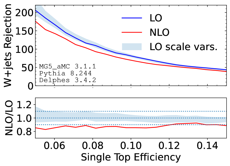
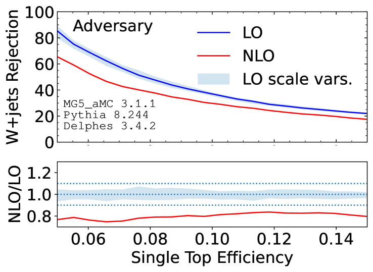
Figure 6: Top: the performance of the nominal $t$-channel single top versus $W$+jets classifier. The blue band represents the uncertainty estimated by varying the factorization scale by $\frac{1}{2}$ and 2 at LO. Bottom: the same as the top, but for the adversarially trained classifier. Adversarial training only reduces the difference in performance to factorization scale variations, not the difference to NLO, indicating that adversarial training provides a reduced estimate of the true uncertainty, which does not translate to a reduction in the true uncertainty.

4 Conclusions and Outlook

Decorrelation is a powerful tool for ensuring that machine learning classifiers can be used in practice to enhance analysis sensitivity. However, this tool must be used with caution. We have shown that decorrelation methods may result in significantly underestimated theory uncertainties when using standard approaches to theory uncertainty estimation. In the cases we explored, the estimated uncertainty uses two samples while the ‘true’ uncertainty relies on a third sample that is not part of the training. One could potentially incorporate the third sample into the decorrelation procedure, but there will always be another variation that is not part of the training as long as the full theory uncertainty decomposition is not known. Until we know the complete set of theory nuisance parameters, it seems prudent to not decorrelate away these uncertainties.

While this paper explicitly studied the case for decorrelation, this cautionary tale remains relevant for other uncertainty or inference aware machine learning approaches Ghosh:2021roe ; Wunsch:2020iuh ; Elwood:2020pik ; Xia:2018kgd ; deCastro:2018mgh ; Charnock_2018 ; Alsing:2019dvb ; lukas_heinrich_2020_3697981 ; Brehmer:2019xox ; Brehmer:2018hga ; Brehmer:2018kdj ; Brehmer:2018eca ; Nachman:2019dol if they are being considered for such theory uncertainties.

Appendix A Training with $\lambda=0$

Figures 7 and 8 show the impact of using the adversarial setup, but with $\lambda=0$, i.e. the adversary is turned off. The only difference with respect to the nominal configuration is that Pythia and Herwig (factorization scale variations) are used instead of just Pythia ($\mu=1$) for the nominal for the two-point (continuous) uncertainty example.

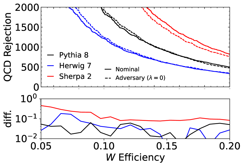
Figure 7: ROC curves for the fragmentation modeling example (Sec. 3.1) with the nominal configuration and for an adversary with $\lambda=0$. The lower panel is the absolute relative difference for each sample between the nominal and adversarial setup.

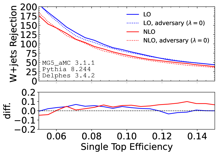
Figure 8: ROC curves for the $t$-channel single top example (Sec. 3.2) with the nominal configuration and for an adversary with $\lambda=0$. The lower panel is the relative difference for each sample between the nominal and adversarial setup.

References

- (1) A. J. Larkoski, I. Moult and B. Nachman, Jet Substructure at the Large Hadron Collider: A Review of Recent Advances in Theory and Machine Learning, Phys. Rept. 841 (2020) 1–63, [1709.04464].
- (2) D. Guest, K. Cranmer and D. Whiteson, Deep Learning and its Application to LHC Physics, Ann. Rev. Nucl. Part. Sci. 68 (2018) 161–181, [1806.11484].
- (3) K. Albertsson et al., Machine Learning in High Energy Physics Community White Paper, 1807.02876.
- (4) A. Radovic, M. Williams, D. Rousseau, M. Kagan, D. Bonacorsi, A. Himmel et al., Machine learning at the energy and intensity frontiers of particle physics, Nature 560 (2018) 41–48.
- (5) G. Carleo, I. Cirac, K. Cranmer, L. Daudet, M. Schuld, N. Tishby et al., Machine learning and the physical sciences, Rev. Mod. Phys. 91 (2019) 045002, [1903.10563].
- (6) D. Bourilkov, Machine and Deep Learning Applications in Particle Physics, Int. J. Mod. Phys. A 34 (2020) 1930019, [1912.08245].
- (7) M. D. Schwartz, Modern Machine Learning and Particle Physics, 2103.12226.
- (8) M. Feickert and B. Nachman, A Living Review of Machine Learning for Particle Physics, 2102.02770.
- (9) B. Nachman, A guide for deploying Deep Learning in LHC searches: How to achieve optimality and account for uncertainty, SciPost Phys. 8 (2020) 090, [1909.03081].
- (10) A. Ghosh, B. Nachman and D. Whiteson, Uncertainty Aware Learning for High Energy Physics, 2105.08742.
- (11) K. Cranmer, J. Pavez and G. Louppe, Approximating Likelihood Ratios with Calibrated Discriminative Classifiers, 1506.02169.
- (12) P. Baldi, K. Cranmer, T. Faucett, P. Sadowski and D. Whiteson, Parameterized neural networks for high-energy physics, Eur. Phys. J. C76 (2016) 235, [1601.07913].
- (13) G. Louppe, M. Kagan and K. Cranmer, Learning to Pivot with Adversarial Networks, Advances in Neural Information Processing Systems 30 (2017) 981, [1611.01046].
- (14) J. Dolen, P. Harris, S. Marzani, S. Rappoccio and N. Tran, Thinking outside the ROCs: Designing Decorrelated Taggers (DDT) for jet substructure, JHEP 05 (2016) 156, [1603.00027].
- (15) I. Moult, B. Nachman and D. Neill, Convolved Substructure: Analytically Decorrelating Jet Substructure Observables, JHEP 05 (2018) 002, [1710.06859].
- (16) J. Stevens and M. Williams, uBoost: A boosting method for producing uniform selection efficiencies from multivariate classifiers, JINST 8 (2013) P12013, [1305.7248].
- (17) C. Shimmin, P. Sadowski, P. Baldi, E. Weik, D. Whiteson, E. Goul et al., Decorrelated Jet Substructure Tagging using Adversarial Neural Networks, Phys. Rev. D 96 (2017) 074034, [1703.03507].
- (18) L. Bradshaw, R. K. Mishra, A. Mitridate and B. Ostdiek, Mass Agnostic Jet Taggers, SciPost Phys. 8 (2020) 011, [1908.08959].
- (19) ATLAS collaboration, Performance of mass-decorrelated jet substructure observables for hadronic two-body decay tagging in ATLAS, Tech. Rep. ATL-PHYS-PUB-2018-014, CERN, Geneva, Jul, 2018.
- (20) G. Kasieczka and D. Shih, Robust Jet Classifiers through Distance Correlation, Phys. Rev. Lett. 125 (2020) 122001, [2001.05310].
- (21) L.-G. Xia, QBDT, a new boosting decision tree method with systematical uncertainties into training for High Energy Physics, Nucl. Instrum. Meth. A930 (2019) 15–26, [1810.08387].
- (22) C. Englert, P. Galler, P. Harris and M. Spannowsky, Machine Learning Uncertainties with Adversarial Neural Networks, Eur. Phys. J. C79 (2019) 4, [1807.08763].
- (23) S. Wunsch, S. Jörger, R. Wolf and G. Quast, Reducing the dependence of the neural network function to systematic uncertainties in the input space, Comput. Softw. Big Sci. 4 (2020) 5, [1907.11674].
- (24) A. Rogozhnikov, A. Bukva, V. Gligorov, A. Ustyuzhanin and M. Williams, New approaches for boosting to uniformity, JINST 10 (2015) T03002, [1410.4140].
- (25) C. Collaboration, A deep neural network to search for new long-lived particles decaying to jets, Machine Learning: Science and Technology (2020) , [1912.12238].
- (26) J. M. Clavijo, P. Glaysher and J. M. Katzy, Adversarial domain adaptation to reduce sample bias of a high energy physics classifier, 2005.00568.
- (27) G. Kasieczka, B. Nachman, M. D. Schwartz and D. Shih, Automating the ABCD method with machine learning, Phys. Rev. D 103 (2021) 035021, [2007.14400].
- (28) O. Kitouni, B. Nachman, C. Weisser and M. Williams, Enhancing searches for resonances with machine learning and moment decomposition, JHEP 21 (2020) 070, [2010.09745].
- (29) B. Andersson, G. Gustafson, G. Ingelman and T. Sjostrand, Parton Fragmentation and String Dynamics, Phys. Rept. 97 (1983) 31–145.
- (30) T. Sjostrand, Jet Fragmentation of Nearby Partons, Nucl. Phys. B 248 (1984) 469–502.
- (31) T. Sjostrand, S. Mrenna and P. Z. Skands, PYTHIA 6.4 Physics and Manual, JHEP 05 (2006) 026, [hep-ph/0603175].
- (32) T. Sjostrand, S. Mrenna and P. Z. Skands, A Brief Introduction to PYTHIA 8.1, Comput. Phys. Commun. 178 (2008) 852–867, [0710.3820].
- (33) B. R. Webber, A QCD Model for Jet Fragmentation Including Soft Gluon Interference, Nucl. Phys. B 238 (1984) 492–528.
- (34) J.-C. Winter, F. Krauss and G. Soff, A Modified cluster hadronization model, Eur. Phys. J. C 36 (2004) 381–395, [hep-ph/0311085].
- (35) J. Bellm et al., Herwig 7.0/Herwig++ 3.0 release note, Eur. Phys. J. C 76 (2016) 196, [1512.01178].
- (36) M. Bahr et al., Herwig++ Physics and Manual, Eur. Phys. J. C 58 (2008) 639–707, [0803.0883].
- (37) S. Chang, T. Cohen and B. Ostdiek, What is the Machine Learning?, Phys. Rev. D 97 (2018) 056009, [1709.10106].
- (38) L. de Oliveira, M. Kagan, L. Mackey, B. Nachman and A. Schwartzman, Jet-Images – Deep Learning Edition., JHEP 07 (2016) 069, [1511.05190].
- (39) G. J. Székely, M. L. Rizzo and N. K. Bakirov, Measuring and testing dependence by correlation of distances, Ann. Statist. 35 (2007) 2769–2794.
- (40) G. J. Székely and M. L. Rizzo, Brownian distance covariance, Ann. Appl. Stat. 3 (2009) 1236–1265.
- (41) G. J. Székely and M. L. Rizzo, The distance correlation t-test of independence in high dimension, J. Multivar. Anal. 117 (2013) 193–213.
- (42) G. J. Székely and M. L. Rizzo, Partial distance correlation with methods for dissimilarities, Ann. Statist. 42 (2014) 2382–2412.
- (43) F. Chollet, “Keras.” https://github.com/fchollet/keras, 2017.
- (44) M. Abadi, P. Barham, J. Chen, Z. Chen, A. Davis, J. Dean et al., Tensorflow: A system for large-scale machine learning., in OSDI, vol. 16, pp. 265–283, 2016.
- (45) D. Kingma and J. Ba, Adam: A method for stochastic optimization, 1412.6980.
- (46) ATLAS collaboration, M. Aaboud et al., Performance of top-quark and -boson tagging with ATLAS in Run 2 of the LHC, Eur. Phys. J. C 79 (2019) 375, [1808.07858].
- (47) CMS collaboration, A. M. Sirunyan et al., Identification of heavy, energetic, hadronically decaying particles using machine-learning techniques, JINST 15 (2020) P06005, [2004.08262].
- (48) A. Butter et al., The Machine Learning Landscape of Top Taggers, SciPost Phys. 7 (2019) 014, [1902.09914].
- (49) J. Alwall, R. Frederix, S. Frixione, V. Hirschi, F. Maltoni, O. Mattelaer et al., The automated computation of tree-level and next-to-leading order differential cross sections, and their matching to parton shower simulations, JHEP 07 (2014) 079, [1405.0301].
- (50) R. D. Ball et al., Parton distributions with LHC data, Nucl. Phys. B 867 (2013) 244–289, [1207.1303].
- (51) T. Gleisberg, S. Hoeche, F. Krauss, M. Schonherr, S. Schumann, F. Siegert et al., Event generation with SHERPA 1.1, JHEP 02 (2009) 007, [0811.4622].
- (52) Sherpa collaboration, E. Bothmann et al., Event Generation with Sherpa 2.2, SciPost Phys. 7 (2019) 034, [1905.09127].
- (53) N. Dawe, E. Rodrigues, H. Schreiner, B. Ostdiek, D. Kalinkin, M. R. et al., scikit-hep/pyjet: Version 1.8.2, Jan., 2021. 10.5281/zenodo.4446849.
- (54) M. Cacciari, G. P. Salam and G. Soyez, FastJet User Manual, Eur. Phys. J. C72 (2012) 1896, [1111.6097].
- (55) M. Cacciari, G. P. Salam and G. Soyez, The anti- jet clustering algorithm, JHEP 04 (2008) 063, [0802.1189].
- (56) J. Thaler and K. Van Tilburg, Identifying Boosted Objects with N-subjettiness, JHEP 03 (2011) 015, [1011.2268].
- (57) J. Thaler and K. Van Tilburg, Maximizing Boosted Top Identification by Minimizing N-subjettiness, JHEP 02 (2012) 093, [1108.2701].
- (58) A. J. Larkoski, I. Moult and D. Neill, Power Counting to Better Jet Observables, JHEP 12 (2014) 009, [1409.6298].
- (59) A. J. Larkoski, G. P. Salam and J. Thaler, Energy Correlation Functions for Jet Substructure, JHEP 06 (2013) 108, [1305.0007].
- (60) Particle Data Group, Review of Particle Physics, Progress of Theoretical and Experimental Physics 2020 (08, 2020) .
- (61) J. M. Butterworth, A. R. Davison, M. Rubin and G. P. Salam, Jet substructure as a new Higgs search channel at the LHC, Phys. Rev. Lett. 100 (2008) 242001, [0802.2470].
- (62) S. D. Ellis, C. K. Vermilion and J. R. Walsh, Recombination Algorithms and Jet Substructure: Pruning as a Tool for Heavy Particle Searches, Phys. Rev. D 81 (2010) 094023, [0912.0033].
- (63) D. Krohn, J. Thaler and L.-T. Wang, Jet Trimming, JHEP 02 (2010) 084, [0912.1342].
- (64) M. Dasgupta, A. Fregoso, S. Marzani and G. P. Salam, Towards an understanding of jet substructure, JHEP 09 (2013) 029, [1307.0007].
- (65) A. J. Larkoski, S. Marzani, G. Soyez and J. Thaler, Soft Drop, JHEP 05 (2014) 146, [1402.2657].
- (66) Y. Ganin and V. Lempitsky, Unsupervised domain adaptation by backpropagation, Proceedings of Machine Learning Research 37 (07–09 Jul, 2015) 1180–1189.
- (67) ATLAS collaboration, M. Aaboud et al., Measurement of the inclusive cross-sections of single top-quark and top-antiquark -channel production in collisions at = 13 TeV with the ATLAS detector, JHEP 04 (2017) 086, [1609.03920].
- (68) CMS collaboration, A. M. Sirunyan et al., Measurement of differential cross sections and charge ratios for t-channel single top quark production in proton–proton collisions at , Eur. Phys. J. C 80 (2020) 370, [1907.08330].
- (69) DELPHES 3 collaboration, J. de Favereau, C. Delaere, P. Demin, A. Giammanco, V. Lemaitre, A. Mertens et al., DELPHES 3, A modular framework for fast simulation of a generic collider experiment, JHEP 02 (2014) 057, [1307.6346].
- (70) A. Mertens, New features in Delphes 3, J. Phys. Conf. Ser. 608 (2015) 012045.
- (71) M. Selvaggi, DELPHES 3: A modular framework for fast-simulation of generic collider experiments, J. Phys. Conf. Ser. 523 (2014) 012033.
- (72) M. Cacciari and G. P. Salam, Dispelling the myth for the jet-finder, Phys. Lett. B641 (2006) 57, [hep-ph/0512210].
- (73) S. Wunsch, S. Jörger, R. Wolf and G. Quast, Optimal statistical inference in the presence of systematic uncertainties using neural network optimization based on binned Poisson likelihoods with nuisance parameters, Comput. Softw. Big Sci. 5 (2021) 4, [2003.07186].
- (74) A. Elwood, D. Krücker and M. Shchedrolosiev, Direct optimization of the discovery significance in machine learning for new physics searches in particle colliders, J. Phys. Conf. Ser. 1525 (2020) 012110.
- (75) P. De Castro and T. Dorigo, INFERNO: Inference-Aware Neural Optimisation, Comput. Phys. Commun. 244 (2019) 170–179, [1806.04743].
- (76) T. Charnock, G. Lavaux and B. D. Wandelt, Automatic physical inference with information maximizing neural networks, Physical Review D 97 (Apr, 2018) .
- (77) J. Alsing and B. Wandelt, Nuisance hardened data compression for fast likelihood-free inference, Mon. Not. Roy. Astron. Soc. 488 (2019) 5093–5103, [1903.01473].
- (78) L. Heinrich and N. Simpson, pyhf/neos: initial zenodo release, Mar., 2020. 10.5281/zenodo.3697981.
- (79) J. Brehmer, F. Kling, I. Espejo and K. Cranmer, MadMiner: Machine learning-based inference for particle physics, Comput. Softw. Big Sci. 4 (2020) 3, [1907.10621].
- (80) J. Brehmer, G. Louppe, J. Pavez and K. Cranmer, Mining gold from implicit models to improve likelihood-free inference, Proc. Nat. Acad. Sci. (2020) 201915980, [1805.12244].
- (81) J. Brehmer, K. Cranmer, G. Louppe and J. Pavez, Constraining Effective Field Theories with Machine Learning, Phys. Rev. Lett. 121 (2018) 111801, [1805.00013].
- (82) J. Brehmer, K. Cranmer, G. Louppe and J. Pavez, A Guide to Constraining Effective Field Theories with Machine Learning, Phys. Rev. D 98 (2018) 052004, [1805.00020].