Standard Errors for Calibrated Parameters

Abstract:

Calibration, the practice of choosing the parameters of a structural model to match certain empirical moments, can be viewed as minimum distance estimation. Existing standard error formulas for such estimators require a consistent estimate of the correlation structure of the empirical moments, which is often unavailable in practice. Instead, the variances of the individual empirical moments are usually readily estimable. Using only these variances, we derive conservative standard errors and confidence intervals for the structural parameters that are valid even under the worst-case correlation structure. In the over-identified case, we show that the moment weighting scheme that minimizes the worst-case estimator variance amounts to a moment selection problem with a simple solution. Finally, we develop tests of over-identifying or parameter restrictions. We apply our methods empirically to a model of menu cost pricing for multi-product firms and to a heterogeneous agent New Keynesian model.

Keywords: calibration, data combination, minimum distance, moment selection, semidefinite programming. JEL codes: C12, C52.

1 Introduction

Researchers often discipline the parameters of structural economic models by calibrating certain model-implied moments to the corresponding moments in the data (Kydland & Prescott, 1996; Nakamura & Steinsson, 2018). In this paper, we follow Hansen & Heckman (1996) and Thomas Sargent (quoted in Evans & Honkapohja, 2005, p. 568) and take the term “calibration” to be synonymous with moment matching (or more generally, minimum distance) estimation. Moment matching estimators are popular in diverse fields of applied structural economics.

Standard moment matching inference requires knowledge of the entire variance-covariance matrix of the empirical moments, but in practice this matrix is often only partially known. When the empirical moments are obtained from different data sets, different econometric methods, or different previous papers, it is usually hard or impossible to estimate the off-diagonal elements of the variance-covariance matrix. Nevertheless, the diagonal of the matrix—the variances of the individual empirical moments—is typically estimable. In this paper, we show that the diagonal suffices to obtain practically useful worst-case standard errors for the moment matching estimator. Moreover, in the over-identified case, we show that the moment weighting that minimizes the worst-case estimator variance amounts to a moment selection problem with a simple solution. Hence, our limited-information methods allow researchers to choose their moments and data sources freely without giving up on doing valid statistical inference.

We show that worst-case standard errors for the structural parameters (or smooth transformations thereof), using only the empirical moment variances, are easy to compute. They are given by a weighted sum of the standard errors of individual empirical moments, where the weights depend on the moment weight matrix and the derivatives of the moments with respect to the structural parameters. The derivatives can be obtained analytically, by automatic differentiation, or by first differences. Using these worst-case standard errors, one can construct a confidence interval that is valid even under the worst-case correlation structure. The confidence interval is generally conservative for specific correlation structures, but its minimax coverage is exact, i.e., under the worst-case correlation structure, which amounts to perfect positive/negative correlation. The confidence interval is likely to be informative in many empirical applications, as it is at most $\sqrt{p}$ times wider than it would be if the moments were known to be independent, where $p$ is the number of moments used for estimation.

Given knowledge of only the individual empirical moment variances, we show that the moment weighting scheme that minimizes the worst-case estimator variance amounts to a moment selection problem. That is, the efficient minimum distance weight matrix attaches zero weight to some of the moments. The efficient selection of moments can be conveniently computed by running a median regression (i.e., Least Absolute Deviation regression) on a particular artificial data set. Our limited-information efficient estimator given knowledge of only the moment variances is generally different from the familiar full-information efficient estimator that requires knowledge of the entire moment correlation structure.

To understand the intuition behind our efficiency result, consider the analogy of portfolio selection in finance. This analogy is mathematically relevant, as it is well known that any minimum distance estimator is asymptotically equivalent to a linear combination of the empirical moments—a “portfolio” of moments—with a linear restriction on the weights to ensure unbiasedness. When constructing a minimum-variance financial portfolio that achieves a given expected return, it is usually optimal to diversify across all available assets, except if the assets are perfectly (positively or negatively) correlated. In the latter extreme case, it is optimal to entirely disregard assets with sufficiently high variance relative to their expected return. But it is precisely the extreme case of perfect correlation that delivers the worst-case variance of a given portfolio. Thus, the portfolio with the smallest worst-case variance across correlation structures is a portfolio that selects a subset of the available assets.

We propose joint tests of parameter restrictions as well as tests of over-identifying restrictions. A common form of over-identification test used in the empirical literature is to check whether the estimated structural parameters yield a good fit of the model to “non-targeted” moments, i.e., moments that were not exploited for parameter estimation. We show how to implement a formal statistical test based on this idea in our setup. For joint testing of parameter restrictions, we propose a Wald-type test. The proof of the validity of this test relies on tail probability bounds for quadratic forms in Gaussian vectors from Székely & Bakirov (2003), but the test statistic and critical value are simple and easy to compute.

Finally, we extend our limited-information procedures to settings with more detailed knowledge of the covariance matrix of empirical moments. This includes settings where the entire correlation structure is known for some subsets of the moments, or where certain moments are known to be independent of each other.

We illustrate the usefulness of our procedures through two empirical applications. In the first one, we estimate and test the Alvarez & Lippi (2014) model of menu cost price setting in multi-product firms, by matching moments of price changes. In the second application, we estimate and test a heterogeneous agent New Keynesian model developed by McKay et al. (2016) and Auclert et al. (2021), by matching impulse responses for macro time series and cross-sectional micro moments. Our worst-case standard errors yield informative inference on several parameters of interest in both applications. A Monte Carlo simulation study calibrated to the first application indicates that our methods perform well in finite samples.

The approach taken in this paper of equating “calibration” with minimum distance estimation is not uncontroversial. Kydland & Prescott (1996) and DeJong & Dave (2011), among others, view “calibration” as a non-econometric procedure for gauging how well a structural macro model fits reduced-form empirical moments. Nevertheless, even in applications where the parameters of the structural model are fixed at values obtained from previous studies, the methods we propose can still be used to compute standard errors for counterfactual quantities and perform tests of the model’s ability to fit additional moments.

Literature.

Unlike the literature on correlation matrix completion, we solve the explicit problem of finding the worst-case correlation structure when estimating parameters in a structural model. Existing papers (see Georgescu et al., 2018, and references therein) instead compute positive definite correlation matrices that satisfy various reduced-form optimality criteria, such as the maximum entropy principle. Our derivations of the worst-case efficient weight matrix and joint testing procedure do not seem to have parallels in the matrix completion literature.

While we focus on cases where it is difficult to estimate the correlation structure of different moments, in some applications it may be possible to model and exploit the precise relationship between the moments. The literature on estimating heterogeneous agent models in macroeconomics has recently developed procedures for combining macro and micro data, as discussed further in Section 5.2. Hahn et al. (2022a, b) provide advanced tools for doing inference with a mix of cross-sectional and time series data. These methods, unlike ours, generally require access to the underlying data. Imbens & Lancaster (1994) consider a microeconometric setting where certain macro moments are known without error, which is a special case of our framework. Hahn et al. (2020) give examples of structural models where both time series and cross-sectional data are required for identification of structural parameters. Their insights may help inform the choice of moments for the methods that we develop below.

Outline.

Section 2 defines the moment matching setup. Section 3 derives the worst-case standard errors and the efficient moment weighting/selection. Section 4 develops tests of parameter restrictions and of over-identifying restrictions. Section 5 contains two empirical illustrations. Section 6 concludes. Appendix A contains proofs and other technical details. Code for implementing our procedures is available online.

2 Setup

Consider a standard moment matching (minimum distance) estimation framework. Let $\mu_{0}\in\mathbb{R}^{p}$ be a vector of reduced-form parameters, which we will refer to as “moments”, though the method applies more generally. Let $\theta_{0}\in\Theta\subset\mathbb{R}^{k}$ be a vector of structural model parameters. According to an economic model, the two parameter vectors are linked by the relationship $\mu_{0}=h(\theta_{0})$, where $h\colon\Theta\to\mathbb{R}^{p}$ is a known function implied by the model. The map $h(\cdot)$ may be computed either analytically or numerically. We have access to an estimator $\hat{\mu}$ (“empirical moments”) that satisfies

$$\sqrt{n}(\hat{\mu}-\mu_{0})\stackrel{{\scriptstyle d}}{{\to}}N(0,V)$$ (1)

for a $p\times p$ symmetric positive semidefinite variance-covariance matrix $V$. Let $\hat{W}$ be a $p\times p$ symmetric matrix satisfying $\hat{W}\stackrel{{\scriptstyle p}}{{\to}}W$ (we discuss the choice of $\hat{W}$ in Section 3.2). Then a “moment matching” or “minimum distance” estimator of $\theta_{0}$ is given by

$$\hat{\theta}=\operatorname*{argmin}_{\theta\in\Theta}\;(\hat{\mu}-h(\theta))^{\prime}\hat{W}(\hat{\mu}-h(\theta)).$$ (2)

This estimation strategy is sometimes referred to as “calibration”.

If we were able to estimate the covariance matrix of the empirical moments $\hat{\mu}$ consistently, it would be straight-forward to construct standard errors for any smooth function of the estimator $\hat{\theta}$. Suppose we are interested in the scalar transformed parameter $r(\theta_{0})$, where $r\colon\Theta\to\mathbb{R}$. For example, $r(\cdot)$ may equal a particular counterfactual quantity in the structural model, or we could simply set $r(\theta)=\theta_{i}$ for some index $i$. Under the standard regularity conditions listed below in Assumption 1,

$$\sqrt{n}(r(\hat{\theta})-r(\theta_{0})) =\lambda^{\prime}(G^{\prime}WG)^{-1}G^{\prime}W\sqrt{n}(\hat{\mu}-\mu_{0})+o_{p}(1)$$ (3)

$$\stackrel{{\scriptstyle d}}{{\to}}N\left(0,\lambda^{\prime}(G^{\prime}WG)^{-1}G^{\prime}WVWG(G^{\prime}WG)^{-1}\lambda\right),$$

where $G\equiv\partial h(\theta_{0})/\partial\theta^{\prime}\in\mathbb{R}^{p\times k}$ and $\lambda\equiv\partial r(\theta_{0})/\partial\theta\in\mathbb{R}^{k}$. See Newey & McFadden (1994) for details. If the entire asymptotic covariance matrix $V$ of $\hat{\mu}$ were consistently estimable, the above display would allow computation of standard errors, confidence intervals, and hypothesis tests.

Unfortunately, the full correlation structure of $\hat{\mu}$ is difficult or impossible to estimate in certain applications. This may be the case, for example, when the moments $\hat{\mu}$ are obtained from a variety of different data sources or econometric methods, or from previous studies for which the underlying data is not readily available. Moreover, if the moments involve a mix of time series and cross-sectional data sources, it can be difficult conceptually or practically to estimate correlations across data sources, whether through the bootstrap or the Generalized Method of Moments (GMM). While the structural model could in some cases be exploited to estimate the moment covariance matrix, this may require stronger assumptions than what is needed for point estimation of the structural parameters. We discuss these points in more detail at the end of this subsection and in the empirical applications in Section 5.

Yet, it is often the case that the standard errors of each of the components of $\hat{\mu}$ are available. These marginal standard errors may be directly computable from data, or they may be reported in the various papers that the individual elements of $\hat{\mu}$ are gleaned from. Thus, assume that we have access to standard errors $\hat{\sigma}_{1},\dots,\hat{\sigma}_{p}\geq 0$ satisfying

$$\sqrt{n}\hat{\sigma}_{j}\stackrel{{\scriptstyle p}}{{\to}}V_{jj}^{1/2},\quad j=1,\dots,p.$$ (4)

We show in the next section that these marginal standard errors suffice for doing informative inference on $r(\theta_{0})$.

For ease of reference, we summarize our technical assumptions here:

Assumption 1.

1. The empirical moment vector $\hat{\mu}$ is asymptotically normal, as in (1).

2. The standard errors $\hat{\sigma}_{j}$ are consistent, as in (4).

3. $h(\cdot)$ and $r(\cdot)$ are both continuously differentiable in a neighborhood of $\theta_{0}$ (which lies in the interior of $\Theta$), $G\equiv\partial h(\theta_{0})/\partial\theta^{\prime}$ has full column rank, and $\lambda\equiv\partial r(\theta_{0})/\partial\theta\neq 0_{k\times 1}$.

4. $\hat{\theta}\stackrel{{\scriptstyle p}}{{\to}}\theta_{0}$.

5. $\hat{W}\stackrel{{\scriptstyle p}}{{\to}}W$ for a symmetric positive semidefinite matrix $W$.

6. $G^{\prime}WG$ is nonsingular.

Conditions (ii)–(vi) are standard regularity conditions that are satisfied in smooth, identified models (Newey & McFadden, 1994). Note that we allow for the possibility that some moments are known with certainty ($V_{jj}=0$) as in Imbens & Lancaster (1994). We will now discuss the key condition (i).

Discussion of limited information about the correlation structure and the joint normality assumption.

We now provide several examples of situations where it is difficult or impossible to estimate the correlation structure of different types of empirical moments. In cases when the elements of the moment vector $\hat{\mu}$ are obtained from different data sets, the joint normality assumption (1) requires justification. This ensures not only that a normal distribution is the appropriate reference distribution for obtaining critical values, but also that the vector $\hat{\mu}$ can reasonably be viewed as arising from some joint, repeatable experiment for which the given standard errors $\hat{\sigma}_{j}$ capture all sources of uncertainty. The joint normality assumption is most easily understood and justified under a model-based (e.g., shock-based) perspective on uncertainty. In this view, there exists a coherent data generating process with both aggregate and idiosyncratic shocks that affect all of the observed data. The empirical application of Section 5.2 is a prototypical example of this framework, but such applications are not the only use case.

There are several cases in which the joint normality assumption appears reasonable, but estimation of the full moment covariance matrix $V$ could be challenging. For example:

1. The moments are obtained from the same or similar data sets, but the underlying data for some of the moments is not available. For example, some moments may be reported in previous papers that use proprietary data. In this case, traditional full-information inference procedures are inapplicable because it is generally impossible to estimate moment cross-correlations without access to the underlying data. However, as long as we have access to marginal standard errors for each individual moment, our methods can be applied. See Section 5.1 for an empirical example.

2. Some of the moments are computed from aggregate time series and others from panel data spanning similar time periods. If the clustering procedure of the panel data regressions allows for aggregate shocks (such as when clustering by time period or when using the standard error formula from Driscoll & Kraay, 1998), and these aggregate shocks also affect the time series data, then the panel regressions will have correct standard errors but the coefficients may be correlated with the time series moments.

3. The moments stem from time series data observed at various frequencies, or from regional data with various levels of geographic aggregation. While careful econometric analysis may allow the estimation of the full covariance matrix of the moments by appropriately collapsing the sample moment conditions for the higher-frequency or higher-resolution data, this could be cumbersome in practice. This is especially true if there is limited overlap in the time spans of the higher-frequency and lower-frequency data, or in the geographical coverage of the higher-resolution and lower-resolution data.

4. We use a combination of aggregate time series moments and micro moments from surveys, and the latter measure time-invariant parameters that are not affected by macro shocks in the sample. In this case, it is often reasonable to assume that the uncertainty in the micro moments (arising purely from idiosyncratic noise) is uncorrelated with the uncertainty in the macro moments. Similarly, cross-sectional moments obtained from different independent random samples are plausibly uncorrelated with each other. Such extra information about off-diagonal entries of $V$ can be incorporated in our procedures, as shown in Section 3.3.

5. The moments are all computed from the same data set, but using a variety of complicated procedures. While it may in principle be possible to estimate the correlation structure analytically by stacking the first-order conditions for the different estimation procedures into a large GMM moment vector, applied researchers may wish to avoid these complications. The bootstrap offers a simpler approach but is computationally impractical in some cases. In contrast, our analytical inference procedures below only require researchers to obtain standard errors for each estimated moment separately, and these are often outputted automatically by existing software. One may worry about the internal consistency of mixing moments arising from different estimation procedures, in the sense that the models used to compute the various moments could be mutually incompatible (or incompatible with the structural model that the researcher seeks to fit to the moments). This can be tested using the over-identification test that we propose in Section 4.2.

6. The moments are all computed from the same data set, but full-information inference procedures perform poorly in finite samples. As shown by Altonji & Segal (1996), traditional full-information efficient minimum distance estimation, which relies on an estimate $\hat{V}$ of the entire moment variance-covariance matrix $V$, can be subject to severe finite-sample biases in many applications, especially when $p$ is large. Whereas full-information efficient inference requires the entire matrix $V$ to be accurately estimated, our limited-information inference procedures below only require accurate estimates of the diagonal entries.

To be clear, in cases 2–6 above (though not in case 1), full-information inference may be possible in principle, as we have indicated. However, this could be cumbersome to implement in practice and/or suffer from poor finite-sample properties. The limited-information procedures we develop offer applied researchers simpler tools that in many cases provide informative inference about structural parameters. Moreover, the limited-information results could be used as a first step for exploring whether it is worthwhile to expend the extra effort required for full-information inference.

It is important to note that the joint normality assumption (1) may fail in some cases, rendering our methods invalid. For example:

1. We use a combination of aggregate time series moments and micro moments from surveys, but the latter are affected by aggregate macro shocks that shift the whole micro outcome distribution. In this case, standard cross-sectional moments may not even be consistent for the true underlying population moments, since the aggregate shocks do not get averaged out (Hahn et al., 2020, Section 3). Moreover, the usual micro standard errors will not take into account the combined uncertainty in the macro shocks and idiosyncratic micro noise. However, if the effects of macro shocks on micro moments do average out and we appropriately account for all types of uncertainty when computing moments and their standard errors, then our methods below can be applied. We illustrate this empirically in Section 5.2.

2. The data used to compute some of the moments is very heavy tailed, or the estimation procedures are not asymptotically regular. In this case, even marginal normality of the individual empirical moments may fail. We leave extensions to non-normal limit distributions as an interesting topic for future research.

3 Standard errors and moment selection

We first derive the worst-case standard errors for a given choice of moment weight matrix. Then we show that the weighting scheme that minimizes the worst-case standard errors amounts to a moment selection problem with a simple solution.

3.1 Worst-case standard errors and confidence intervals

We first compute the worst-case bound on the standard error of the moment matching estimator, given knowledge of only the variances of the empirical moments. Although the mathematical argument is straight-forward, it appears that the literature has not realized the practical utility of this result.

Recall that we seek to do inference on the scalar parameter $r(\theta_{0})$. By the standard delta method expansion (3) under Assumption 1, the estimator $r(\hat{\theta})$ is asymptotically equivalent to a certain linear function $x^{\prime}\hat{\mu}$ of the empirical moments, where $x=(x_{1},\dots,x_{p})^{\prime}\equiv WG(G^{\prime}WG)^{-1}\lambda$. We thus seek to bound the variance of an (asymptotically) known linear combination of $\hat{\mu}$, knowing the variance of each component $\hat{\mu}_{j}$ but not the correlation structure. This worst-case variance is attained when all components of $\hat{\mu}$ are perfectly positively or negatively correlated (depending on the signs of the elements of $x$), yielding the worst-case variance $(\sum_{j=1}^{p}|x_{j}|\operatorname*{Var}(\hat{\mu}_{j})^{1/2})^{2}$, as is proved in the following elementary lemma.

Lemma 1.

Let $x=(x_{1},\dots,x_{p})^{\prime}\in\mathbb{R}^{p}$ and $\sigma_{1}^{2},\dots,\sigma_{p}^{2}\geq 0$. Let $\mathcal{S}(\sigma)$ denote the set of $p\times p$ symmetric positive semidefinite matrices with diagonal elements $\sigma=(\sigma_{1}^{2},\dots,\sigma_{p}^{2})^{\prime}$. Then

$$\max_{V\in\mathcal{S}(\sigma)}\sqrt{x^{\prime}Vx}=\sum_{j=1}^{p}\sigma_{j}|x_{j}|.$$

Proof.

The right-hand side is attained by $V=ss^{\prime}$, where $s=(\sigma_{1}\operatorname*{sign}(x_{1}),\dots,\sigma_{p}\operatorname*{sign}(x_{p}))^{\prime}$. Moreover, for any $V\in\mathcal{S}(\sigma)$,

$$x^{\prime}Vx=\sum_{j=1}^{p}\sum_{\ell=1}^{p}x_{j}x_{\ell}V_{j\ell}\leq\sum_{j=1}^{p}\sum_{\ell=1}^{p}|x_{j}x_{\ell}|\,|V_{j\ell}|\leq\sum_{j=1}^{p}\sum_{\ell=1}^{p}|x_{j}x_{\ell}|\,\sigma_{j}\sigma_{\ell}=\left(\sum_{j=1}^{p}\sigma_{j}|x_{j}|\right)^{2},$$

where the penultimate inequality uses that $|V_{j\ell}|^{2}\leq V_{jj}V_{\ell\ell}$ for any symmetric positive semidefinite matrix $V$. ∎

We can thus construct an estimate of the worst-case standard error of $r(\hat{\theta})$ as

$$\widehat{\text{se}}(\hat{x})\equiv\sum_{j=1}^{p}\hat{\sigma}_{j}|\hat{x}_{j}|,$$ (5)

where $\hat{x}=(\hat{x}_{1},\dots,\hat{x}_{p})^{\prime}\equiv\hat{W}\hat{G}(\hat{G}^{\prime}\hat{W}\hat{G})^{-1}\hat{\lambda}$, $\hat{G}\equiv\frac{\partial h(\hat{\theta})}{\partial\theta^{\prime}}$, and $\hat{\lambda}\equiv\frac{\partial r(\hat{\theta})}{\partial\theta}$. In practice, the derivatives may be computed analytically, by automatic differentiation, or by finite differences. Let $\Phi(\cdot)$ denote the standard normal distribution function. Then the confidence interval

$$\widehat{\text{CI}}\equiv\left[r(\hat{\theta})-\Phi^{-1}(1-\alpha/2)\widehat{\text{se}}(\hat{x}),r(\hat{\theta})+\Phi^{-1}(1-\alpha/2)\widehat{\text{se}}(\hat{x})\right]$$

covers $r(\theta_{0})$ with probability at least $1-\alpha$ asymptotically, as shown formally in the following proposition. The asymptotic coverage probability generally exceeds $1-\alpha$ due to the worst-case perspective, but coverage is exact in a particular special case when all elements of the empirical moment vector $\hat{\mu}$ are perfectly correlated asymptotically.

Proposition 1.

Impose Assumption 1 and $\max_{j}|x_{j}|V_{jj}>0$. Then $\lim_{n\to\infty}P(r(\theta_{0})\in\widehat{\text{CI}})\geq 1-\alpha$, and the inequality binds for the rank-1 matrix $V$ defined in the proof of Lemma 1.

Proof.

Please see Section A.1. ∎

Remarks.

1. The worst-case standard errors are at most $\sqrt{p}$ times larger than the standard errors that assume all elements of $\hat{\mu}$ to be mutually uncorrelated. This follows from Hölder’s inequality between $\ell_{1}$ and $\ell_{2}$ norms, which yields $\sum_{j=1}^{p}\hat{\sigma}_{j}|\hat{x}_{j}|\leq p^{1/2}(\sum_{j=1}^{p}\hat{\sigma}_{j}^{2}\hat{x}_{j}^{2})^{1/2}$.

2. Though often informative, limited-information inference can potentially have much lower power than full-information inference. Specifically, the worst-case standard errors can in some (but not all) models be arbitrarily larger than the standard errors one would report given full knowledge of $V$. For example, consider a “repeated measurements” model with $k=1$, $p=2$, $h(\theta)=(\theta,\theta)^{\prime}$, $r(\theta)=\theta$, and $\hat{W}=I$, yielding the estimator $\hat{\theta}=(\hat{\mu}_{1}+\hat{\mu}_{2})/2$. The worst-case standard error of $\hat{\theta}$ equals $(\hat{\sigma}_{1}+\hat{\sigma}_{2})/2$, corresponding to the case where $\hat{\mu}_{1}$ and $\hat{\mu}_{2}$ are perfectly positively correlated. But it is easy to verify that the best-case standard error equals $|\hat{\sigma}_{1}-\hat{\sigma}_{2}|/2$, corresponding to $\hat{\mu}_{1}$ and $\hat{\mu}_{2}$ being perfectly negatively correlated. If $\hat{\sigma}_{1}=\hat{\sigma}_{2}$, the ratio of worst-case to best-case standard errors is infinite.

3. In applications where the moment function $h(\theta)$ cannot be evaluated analytically, the moments can instead be approximated by simulating from the economic model given parameter vector $\theta$. Proposition 3 in Section A.2 shows that the conclusions of Proposition 1 continue to apply in this case, as long as the number of simulation draws is sufficiently large relative to the empirical sample size $n$.

3.2 Efficient moment selection

We now derive a weight matrix $W$ that minimizes the worst-case variance of the estimator, derived above. We show that this weight matrix puts weight on at most $k$ moments, so the procedure amounts to efficient moment selection. Since the weight matrix $W$ only matters in the over-identified case, we assume $p>k$ in this section.

We seek a weight matrix $W$ that minimizes the worst-case asymptotic standard deviation of $r(\hat{\theta})$. Let $x(W)$ denote the vector $x$ defined in Section 3.1, viewed as a function of $W$, and let $\mathcal{S}_{p}$ denote the set of $p\times p$ symmetric positive semidefinite matrices $W$ such that $G^{\prime}WG$ is nonsingular. Then we solve the problem

$$\min_{W\in\mathcal{S}_{p}}\max_{\tilde{V}\in\mathcal{S}(\operatorname*{diag}(V))}\sqrt{\lambda^{\prime}(G^{\prime}WG)^{-1}G^{\prime}W\tilde{V}WG(G^{\prime}WG)^{-1}\lambda}$$ (6)

$$\qquad=\min_{W\in\mathcal{S}_{p}}\max_{\tilde{V}\in\mathcal{S}(\operatorname*{diag}(V))}(x(W)^{\prime}\tilde{V}x(W))^{1/2}$$

$$\qquad=\min_{W\in\mathcal{S}_{p}}\;\sum_{j=1}^{p}V_{jj}^{1/2}|x_{j}(W)|,$$

where the last equality uses Lemma 1 in Section 3.1. Lemma 2 in Section A.1 shows that the solution to the final optimization problem above is given by

$$\min_{W\in\mathcal{S}_{p}}\;\sum_{j=1}^{p}V_{jj}^{1/2}|x_{j}(W)|=\min_{z\in\mathbb{R}^{p-k}}\;\sum_{j=1}^{p}|\tilde{Y}_{j}-\tilde{X}_{j}^{\prime}z|,$$ (7)

where we define

$$\tilde{Y}_{j}\equiv V_{jj}^{1/2}G_{j\bullet}(G^{\prime}G)^{-1}\lambda\in\mathbb{R},\quad\tilde{X}_{j}\equiv-V_{jj}^{1/2}G_{j\bullet}^{\perp\prime}\in\mathbb{R}^{p-k},$$

$G^{\perp}$ is any $p\times(p-k)$ matrix with full column rank satisfying $G^{\prime}G^{\perp}=0_{k\times(p-k)}$, and the notation $A_{j\bullet}$ means the $j$-th row of matrix $A$. The intuition for the equality (7) is that the set of all minimum distance estimators for various weight matrices is asymptotically equivalent to the set of all estimators that are linear combinations of the $p$ moments $\hat{\mu}$, subject to $k$ asymptotic unbiasedness constraints. We can therefore optimize over a $(p-k)$-dimensional linear space.

The final optimization problem (7) is a median regression (Least Absolute Deviation regression) of the artificial “regressand” $\{\tilde{Y}_{j}\}$ on the $p-k$ artificial “regressors” $\{\tilde{X}_{j}\}$. This regression can be executed efficiently using standard quantile regression software.

The solution to the median regression amounts to optimally selecting at most $k$ of the $p$ moments for estimation. Theorem 3.1 of Koenker & Bassett (1978) implies that there exists a solution $z^{*}$ to the median regression (7) such that at least $p-k$ out of the $p$ median regression residuals

$$e_{j}^{*}\equiv\tilde{Y}_{j}-\tilde{X}_{j}^{\prime}z^{*},\quad j=1,\dots,p,$$

equal zero. Hence, an efficient weight matrix $W^{*}$ that achieves the minimum in (7) will yield a linear combination vector $x(W^{*})=(V_{11}^{-1/2}e_{1}^{*},\dots,V_{pp}^{-1/2}e_{p}^{*})^{\prime}$ that attaches nonzero weight to at most $k$ out of the $p$ empirical moments $\hat{\mu}$. In other words, the solution to the efficient moment weighting problem is endogenously achieved by an efficient moment selection. We may pick an arbitrary weight matrix that attaches nonzero weight to only the efficiently selected moments (the magnitudes of the weights do not matter asymptotically, as the selected set of moments is just-identified).

Analytical illustration.

To illustrate the above results, and to link back to the intuitive discussion of portfolio selection in Section 1, consider a “repeated measurements” model with $k=1$, $p=2$, $h(\theta)=(\theta,\theta)^{\prime}$, and $r(\theta)=\theta$. It is easy to see that any weight matrix $\hat{W}$ yields a minimum distance estimator of the form $\hat{\theta}=x_{1}\hat{\mu}_{1}+x_{2}\hat{\mu}_{2}$, where $x_{1}+x_{2}=1$. The constraint that $x_{1}$ and $x_{2}$ sum to 1 ensures that the estimator is consistent. The choice of optimal weight matrix corresponds to an optimal choice of $x_{1}$ and $x_{2}=1-x_{1}$. One might expect the usual diversification motive to cause us to attach nonzero weights to both empirical moments $\hat{\mu}_{1}$ and $\hat{\mu}_{2}$, so that their estimation errors average out partially. However, for the worst-case correlation structure for these moments—perfect correlation—their estimation errors amplify each other, rendering diversification futile. Hence, we minimize the worst-case standard error $|x_{1}|\hat{\sigma}_{1}+|1-x_{1}|\hat{\sigma}_{2}$ by setting $x_{1}=1$ when $\hat{\sigma}_{1}<\hat{\sigma}_{2}$ and otherwise $x_{1}=0$, yielding the estimator $\hat{\theta}=\hat{\mu}_{\operatorname*{argmin}_{j}\hat{\sigma}_{j}}$. That is, the efficient estimator simply discards the moment with the largest standard error. In more general models, moment selection also depends on how informative each moment is about the structural parameters, as measured by the Jacobian matrix $G$.

Algorithm.

The efficient estimator and standard errors can be computed as follows:

1. Compute an initial $\sqrt{n}$-consistent estimator $\hat{\theta}_{\text{init}}$ using, say, a diagonal weight matrix with $\hat{W}_{jj}=\hat{\sigma}_{j}^{-2}$.

2. Construct the derivative matrix $\hat{G}\equiv\frac{\partial h(\hat{\theta}_{\text{init}})}{\partial\theta^{\prime}}$ and vector $\hat{\lambda}\equiv\frac{\partial r(\hat{\theta}_{\text{init}})}{\partial\theta}$, either analytically or numerically.

3. Solve the median regression (7), substituting $\hat{G}$ for $G$, $\hat{\lambda}$ for $\lambda$, and $\hat{\sigma}_{j}$ for $V_{jj}^{1/2}$. Compute the residuals $\hat{e}_{j}^{*}$, $j=1,\dots,p$, from this median regression. (In the non-generic case where multiple solutions to the median regression exist, select one that yields at most $k$ nonzero residuals.)

4. Construct the efficient linear combination $\hat{x}^{*}=(\hat{x}_{1}^{*},\dots,\hat{x}_{p}^{*})^{\prime}$ of the $p$ moments, given by $\hat{x}_{j}^{*}\equiv\hat{\sigma}_{j}^{-1}\hat{e}_{j}^{*}$ for $j=1,\dots,p$. At least $p-k$ of the elements will be zero, corresponding to those moments that are discarded by the efficient moment selection procedure.

5. To compute an efficient estimator of $r(\theta_{0})$, either:

   1. Compute the just-identified efficient minimum distance estimator $\hat{\theta}_{\text{eff}}$ of $\theta_{0}$ which uses any weight matrix that attaches zero weight to those (at least) $p-k$ moments which receive zero weight in the vector $\hat{x}^{*}$. Then estimate $r(\theta_{0})$ by $r(\hat{\theta}_{\text{eff}})$. Or:

   2. Compute the “one-step” estimator $\hat{r}_{\text{eff-1S}}\equiv r(\hat{\theta}_{\text{init}})+\hat{x}^{*}{}^{\prime}(\hat{\mu}-h(\hat{\theta}_{\text{init}}))$ of $r(\theta_{0})$.

6. The worst-case standard error of the estimator from step (v) is given by the value of the median regression (7) (i.e., the minimized objective function).

Options (a) and (b) in step (v) of the algorithm are asymptotically equivalent. Option (b) is computationally more convenient as it avoids further numerical optimization, but option (a) ensures that $\hat{\theta}_{\text{eff}}$ always lies in the parameter space $\Theta$.

Remarks.

1. Since all operations involved in computing the efficient linear combination $\hat{x}^{*}$ are continuous, $\hat{x}^{*}$ converges in probability to the population efficient linear combination $x(W^{*})$. The only exception may be where the population median regression (7) does not have a unique minimum, which is a non-generic case. Even in this case, however, the efficient worst-case standard errors will be consistent (when multiplied by $\sqrt{n}$) under Assumption 1(i)–(iv), by a standard application of the maximum theorem.

2. The full-information (infeasible) efficient weight matrix that exploits knowledge of all of $V$ is known to equal $W=V^{-1}$. This weight matrix in general attaches nonzero weight to all moments, unlike the limited-information efficient solution derived above. The worst-case asymptotic standard deviation (7) given limited information is of course larger than the asymptotic standard deviation $(\lambda^{\prime}(G^{\prime}V^{-1}G)^{-1}\lambda)^{1/2}$ of the full-information efficient estimator of $r(\theta_{0})$.

3. The efficient moment weighting/selection for the limited-information efficient estimators $r(\hat{\theta}_{\text{eff}})$ and $\hat{r}_{\text{eff-1S}}$ depends on the function $r(\cdot)$ of interest, unlike in the case of full-information efficient estimation. In practice, we can just re-run the computations for each function $r(\cdot)$ of interest (e.g., for each component of $\theta$).

4. By restricting $W$ to the set $\mathcal{S}_{p}$ of weight matrices for which $G^{\prime}WG$ is nonsingular, we ensure that the parameter vector $\theta_{0}$ is at least locally identified from the selected moments (Newey & McFadden, 1994, p. 2144). However, the selected moments may fail to ensure global identification of $\theta_{0}$. In models for which this is a concern, we recommend using the one-step efficient estimator $\hat{r}_{\text{eff-1S}}$, which inherits its consistency from the initial estimator $\hat{\theta}_{\text{init}}$ that could be computed using all available moments.

5. It is not restrictive to consider moment matching estimators of the form (2). Consider instead any estimator $\hat{\vartheta}\equiv\hat{f}(\hat{\mu})$ of $\theta_{0}$, where $\hat{f}\colon\mathbb{R}^{p}\to\mathbb{R}^{k}$ is a possibly data-dependent function with enough regularity to satisfy the asymptotically linear expansion

   $$\hat{\vartheta}-\theta_{0}=H(\hat{\mu}-\mu_{0})+o_{p}(n^{-1/2}),$$

   for some $k\times p$ matrix $H$. If we restrict attention to asymptotically regular estimators of $\theta_{0}$ (i.e., estimators that remain asymptotically unbiased under locally drifting parameters), we need $HG=I_{k}$. Among all estimators $\hat{\vartheta}$ satisfying these requirements, the smallest possible worst-case asymptotic standard deviation of $r(\hat{\vartheta})$ is achieved by the estimator whose asymptotic linearization matrix $H$ solves

   $$\min_{H\colon HG=I_{k}}\;\max_{\tilde{V}\in\mathcal{S}(\operatorname*{diag}(V))}(\lambda^{\prime}H^{\prime}\tilde{V}H\lambda)^{1/2}.$$

   Lemma 2 in Section A.1 shows that the solution to this problem is precisely the value of the median regression (7). In other words, the minimum distance estimator $\hat{\theta}$ with (limited-information) efficient weight matrix delivers the smallest possible worst-case standard errors in a large class of estimators.

3.3 General knowledge of the covariance matrix

We now extend our results to the general case where any collection of elements of the asymptotic covariance matrix $V$ of the moments $\hat{\mu}$ is known (or consistently estimable), while the remaining elements are unrestricted. For example, if a pair of elements of $\hat{\mu}$ are known to be independent, the corresponding off-diagonal elements of $V$ must equal zero.

Letting $\tilde{\mathcal{S}}$ denote the given constraint set for $V$, we can compute the worst-case asymptotic standard deviation of $r(\hat{\theta})$ as

$$\sqrt{\max_{\tilde{V}\in\tilde{\mathcal{S}}}\,x^{\prime}\tilde{V}x},$$ (8)

where $x$ was defined in Section 3.1. In the case of interest to us, $\tilde{\mathcal{S}}$ is defined by equality restrictions on a subset of the elements of $V$, in addition to the restriction that $V$ is symmetric positive semidefinite. Then the maximization problem (8) is a so-called semidefinite programming problem, a special case of convex programming. In Section A.3, we show that the efficient weight matrix can likewise be computed through a pair of nested convex optimizations. We also show that analytical simplifications obtain in the special case where we know the block diagonal of $V$; such a structure may occur if consecutive elements of $\hat{\mu}$ are obtained from the same data set, allowing estimation of covariances among these elements. Our software automatically implement all these computations (see Footnote 1).

4 Testing

In this section we develop a joint test of multiple parameter restrictions as well as a test of over-identifying restrictions.

4.1 Joint testing of parameter restrictions

We propose a test of the joint null hypothesis $H_{0}\colon r(\theta_{0})=0_{m\times 1}$ against the two-sided alternative. In this section, the continuously differentiable function $r\colon\Theta\to\mathbb{R}^{m}$ is allowed to be multi-valued. Tests of a single parameter restriction ($m=1$) can be carried out using the confidence interval described in Section 3.1. For the case $m>1$, we propose the following testing procedure. Let $\alpha\in(0,1)$ denote the significance level.

1. Compute the Wald-type test statistic

   $$\hat{\mathscr{T}}\equiv r(\hat{\theta})^{\prime}\hat{S}r(\hat{\theta}),$$

   where $\hat{S}$ is a user-specified symmetric positive definite $m\times m$ matrix, to be discussed below.

2. Compute the critical value

   $$\text{cv}_{n}\equiv\max_{\tilde{V}\in\mathcal{S}(\operatorname*{diag}(V))}\frac{1}{n}\operatorname*{trace}\left(\tilde{V}WG(G^{\prime}WG)^{-1}\lambda S\lambda^{\prime}(G^{\prime}WG)^{-1}G^{\prime}W\right)\times\left(\Phi^{-1}(1-\alpha/2)\right)^{2}.$$ (9)

   In practice, we substitute the estimates $\frac{1}{n}\operatorname*{diag}(V)\approx\operatorname*{diag}(\hat{\sigma}_{1}^{2},\dots,\hat{\sigma}_{p}^{2})$, $W\approx\hat{W}$, $S\approx\hat{S}$, $G\approx\hat{G}\equiv\frac{\partial h(\hat{\theta})}{\partial\theta^{\prime}}$, and $\lambda\approx\hat{\lambda}\equiv\frac{\partial r(\hat{\theta})^{\prime}}{\partial\theta}$.

3. Reject $H_{0}\colon r(\theta_{0})=0_{m\times 1}$ if $\hat{\mathscr{T}}>\text{cv}_{n}$.

The maximization (9) is a semidefinite programming problem, which is easy to compute numerically, as discussed in Section 3.3. Section A.3 extends the procedure to settings where additional knowledge about $V$ is available other than the diagonal.

The following proposition shows that, for conventional significance levels $\alpha$, the asymptotic size of this test does not exceed $\alpha$, regardless of the true correlation structure of the moments. This holds for any valid choice of weight matrix $\hat{W}$, including—but not limited to—the limited-information efficient weight matrix derived in Section 3.2.

Proposition 2.

Impose Assumption 1, except that we redefine $\lambda\equiv\partial r(\theta_{0})^{\prime}/\partial\theta$ and require this matrix to have full column rank $m$. Assume also that $\hat{S}\stackrel{{\scriptstyle p}}{{\to}}S$, $S$ is symmetric positive definite, $n\,\mathrm{cv}_{n}>0$, and $\alpha\leq 0.215$. Then, if $r(\theta_{0})=0_{m\times 1}$,

$$\limsup_{n\to\infty}P(\hat{\mathscr{T}}>\mathrm{cv}_{n})\leq\alpha.$$

Proof.

Please see Section A.1. ∎

Remarks.

1. We do not have formal results on how to choose the weight matrix $\hat{S}$ in the test statistic. A pragmatic ad hoc choice is to set $\hat{S}=(\lambda^{\prime}(G^{\prime}WG)^{-1}G^{\prime}W\bar{V}WG(G^{\prime}WG)^{-1}\lambda)^{-1}$ (with consistent estimates plugged in), where $\bar{V}$ is a particular value for the asymptotic variance $V$ of $\hat{\mu}$ at which we wish to direct power. Then $\hat{\mathscr{T}}$ is the usual full-information Wald statistic given $V=\bar{V}$, though the critical value for the test differs from the conventional one to ensure size control regardless of the actual unknown correlation structure. For example, if we want to direct power toward the case with independent moments, we can choose $\bar{V}=\operatorname*{diag}(n\hat{\sigma}_{1}^{2},\dots,n\hat{\sigma}_{p}^{2})$.

2. The test procedure in Proposition 2 is generally conservative from a minimax perspective, i.e., the size may be strictly smaller than $\alpha$ for all covariance matrices $V$ of the moments. The reason is that the proof of Proposition 2 relies on a tail probability bound for quadratic forms of Gaussian random vectors (Székely & Bakirov, 2003). This bound is attained when $V$ has rank 1, but the positive semidefinite maximum (9) need not be attained at a rank-1 matrix, to our knowledge. It is an interesting topic for future research to devise a test that has a formal minimax optimality property given the limited knowledge of $V$.

3. The test procedure is consistent against any fixed alternative with $r(\theta_{0})\neq 0_{m\times 1}$ under the conditions of Proposition 2. This follows from the standard argument that $n\hat{\mathscr{T}}$ diverges to infinity with probability 1 in this case, while $\text{cv}_{n}=O(n^{-1})$ since the largest eigenvalue of any matrix $\tilde{V}\in\mathcal{S}(\operatorname*{diag}(V))$ is bounded above by $\sum_{j=1}^{p}V_{jj}$.

4. An alternative way to test multiple hypotheses ($m>1$) is to separately test each null hypothesis $r_{j}(\theta_{0})=0$, $j=1,\dots,m$, using the univariate confidence interval for $r_{j}(\theta_{0})$ in Section 3.1, but with a Bonferroni correction applied to the significance level. That is, the test rejects the joint hypothesis when any of the $m$ level-$(1-\alpha/m)$ confidence intervals excludes 0. This Bonferroni test neither dominates, nor is it dominated by, the test in Proposition 2 in terms of local power in general. The latter test has the advantage that it is finite-sample invariant to nonsingular linear transformations of the joint null hypothesis (if $\hat{S}$ is chosen as in the first remark above).

4.2 Over-identification testing

The fit of the calibrated model can be evaluated using over-identification tests when we have more moments $p$ than parameters $k$. In this subsection we allow for potential model misspecification by dropping the assumption in Section 2 that there exists $\theta_{0}\in\mathbb{R}^{k}$ such that $h(\theta_{0})=\mu_{0}$. Let an arbitrary weight matrix $\hat{W}\stackrel{{\scriptstyle p}}{{\to}}W$ be given, such as the limited-information efficient weight matrix derived in Section 3.2. Define the pseudo-true parameter $\tilde{\theta}_{0}\equiv\operatorname*{argmin}_{\theta\in\mathbb{R}^{k}}(\mu_{0}-h(\theta))^{\prime}W(\mu_{0}-h(\theta))$, assuming the minimizer is unique. We continue to impose all the assumptions in Section 2, with $\tilde{\theta}_{0}$ substituting for $\theta_{0}$.

Suppose we want to know whether the model provides a good fit for a particular moment. Let $j^{*}\in\{1,\dots,p\}$ be the index of the moment of interest. We seek a confidence interval for the model misspecification measure $\mu_{0,j^{*}}-h_{j^{*}}(\tilde{\theta}_{0})$, i.e., the $j^{*}$-th element of $\mu_{0}-h(\tilde{\theta}_{0})$. It is standard to show that, under Assumption 1,

$$\hat{\mu}-h(\hat{\theta})-(\mu_{0}-h(\tilde{\theta}_{0}))=(I_{p}-G(G^{\prime}WG)^{-1}G^{\prime}W)(\hat{\mu}-\mu_{0})+o_{p}(n^{-1/2}).$$ (10)

Let $\bar{x}$ be the $j^{*}$-th column of the matrix $I_{p}-\hat{W}\hat{G}(\hat{G}^{\prime}\hat{W}\hat{G})^{-1}\hat{G}^{\prime}$. Then

$$\left[\hat{\mu}_{j^{*}}-h_{j^{*}}(\hat{\theta})-\Phi^{-1}(1-\alpha/2)\widehat{\text{se}}(\bar{x}),\hat{\mu}_{j^{*}}-h_{j^{*}}(\hat{\theta})+\Phi^{-1}(1-\alpha/2)\widehat{\text{se}}(\bar{x})\right]$$

is a confidence interval for the difference $\mu_{0,j^{*}}-h_{j^{*}}(\tilde{\theta}_{0})$, with worst-case asymptotic coverage probability $1-\alpha$. Note that it can happen that $\widehat{\text{se}}(\bar{x})=0$, in which case it is not possible to test the over-identifying restriction corresponding to the $j^{*}$-th moment.

One common use of over-identification testing is to evaluate the estimated model’s fit on “non-targeted moments”. This corresponds to the special case where the weight matrix $\hat{W}$ zeroes out the corresponding rows and columns of the non-targeted moments, so that the point estimate $\hat{\theta}$ ignores these moments. An application of this idea is to fix the structural parameters $\theta$ to values obtained from previous studies and then evaluate whether the model’s predictions at these parameters match additional moments (this can be viewed as a statistical version of the model validation process advocated by Kydland & Prescott, 1996). This is achieved by choosing a moment function of the form $h(\theta)=(\theta^{\prime},\bar{h}(\theta))^{\prime}$, with empirical moments $\hat{\mu}=(\hat{\tilde{\theta}}^{\prime},\hat{\bar{\mu}})^{\prime}$. Here $\hat{\tilde{\theta}}$ are the parameter values obtained from previous studies, while $\bar{h}(\theta)$ is the “non-targeted” model prediction of the empirical moment $\hat{\bar{\mu}}$.

5 Empirical applications

We illustrate our methods through two empirical examples. First we fit a model of menu cost price setting in multi-product firms to scanner data. Then we fit a heterogeneous agent New Keynesian model to impulse responses that have been estimated from a combination of micro and macro data.

5.1 Menu cost price setting in multi-product firms

Our first application estimates the Alvarez & Lippi (2014) model of menu cost price-setting in multiproduct firms. We fit the model to moments of price changes from supermarket scanner data. This is a small-scale application with $k=3$ parameters and $p=4$ moments.

Though we in fact have access to the underlying data set, we emulate a hypothetical situation where the model is matched to moments that were reported in another paper. We can therefore compare full-information inference, which uses the underlying data, with limited-information inference, which uses only the moments and their marginal standard errors. We find that limited-information inference remains informative about the structural parameters. Moreover, a simulation study calibrated to this application confirms the utility of our procedures in finite samples.

Model.

We give a brief overview of the structural model here and refer the reader to Alvarez & Lippi (2014) for details. A firm sets prices on $N$ products. The desired log prices for the products evolve in continuous time as $N$ independent Brownian motions (without drift); however, the actual prices are fixed until the firm pays a fixed menu cost, at which point it may reset all $N$ prices simultaneously. The firm’s profit depends negatively on the squared log deviation between the current and desired price, integrated over time and averaged across the $N$ products. The model has $k=3$ parameters: the number $N$ of products, the volatility of the desired prices, and the scaled menu cost (relative to the curvature of the profit function). Alvarez & Lippi (2014) derive closed-form expressions for the frequency of price changes and the moments of the size of price changes. These are the moments we will match in the data.

Data.

We empirically estimate the frequency and moments of price changes in scanner data from the supermarket chain Dominick’s. As described in detail in Section A.4, we clean the data following Alvarez et al. (2016), and in particular we focus on data from a single store. Unlike those authors, we exclusively use data on beer products, which arguably increases the interpretability of the results and makes the sample size more relevant for our subsequent simulation study. The final data set contains weekly prices on 499 beer products (Universal Product Codes, henceforth UPCs), observed for an average of 76 weeks per UPC. The total sample size is $n=\text{37,916}$. When computing standard errors, we treat the price changes as i.i.d. across UPCs and time.

The $p=4$ reduced-form moments that we match to the structural model are the average number of price changes per week as well as the empirical first, second, and fourth moments of the absolute log price changes (conditional on a nonzero change). We estimate the full-information covariance matrix of these moments using the usual nonparametric estimate (which depends on sample moments of price changes up to order 8). When applying our limited-information procedures, we use only the diagonal of this covariance matrix.

Results.

We consider both just-identified and efficient specifications. We treat the number $N$ of products as a parameter to be estimated, since there may not be a perfect correspondence between a UPC and the structural model’s notion of a “product”. The just-identified specification uses a weight matrix that attaches zero weight to the first moment of absolute price changes (i.e., the average), so that the three parameters are estimated from three moments (this estimator is available in closed form). We can then check whether the model provides a good fit for the “non-targeted” moment by carrying out the over-identification test proposed in Section 4.2. The efficient specification exploits all four empirical moments, using either the conventional full-information one-step estimator or our limited-information one-step estimator in Section 3.2. In addition to the full-information and limited-information procedures, we report results for a procedure that (erroneously) assumes that the four empirical moments are mutually independent.

Price setting application: Parameter estimates
Just-identified specification Efficient specification # prod. Vol. Menu cost Over-ID # prod. Vol. Menu cost Full-info 3.012 0.090 0.291 0.002 3.255 0.089 0.305 (0.046) (0.001) (0.003) (0.000) (0.051) (0.001) (0.003) Independ. 3.012 0.090 0.291 0.002 2.829 0.090 0.280 (0.167) (0.001) (0.010) (0.001) (0.091) (0.000) (0.006) Worst case 3.012 0.090 0.291 0.002 2.786 0.090 0.278 (0.235) (0.001) (0.016) (0.002) (0.148) (0.001) (0.011)

Table 1: Estimates for the just-identified specification (uses only three moments for estimation) and the efficient specification (exploits all four moments for estimation). The rows correspond to full-information inference (exploits knowledge of $\hat{V}$), inference under independence (erroneously assumes that $\hat{V}$ is diagonal), and worst-case inference (exploits only diagonal of $\hat{V}$ without assuming off-diagonal elements are zero). Parameters: number of products (“# prod.”), volatility of desired log price (“Vol.”), scaled menu cost (“Menu cost”). Column “Over-ID” displays the error in fitting the non-targeted mean absolute price change moment, given the just-identified parameter estimates. Standard errors in parentheses.

Table 1 shows that the limited-information standard errors are larger than the full-information ones, but they remain highly informative about the values of the structural parameters. In the efficient over-identified specification, the worst-case standard errors are at most 3.7 times larger than the corresponding full-information values. Importantly, all worst-case standard errors are arguably small relative to the economic magnitudes of the parameter estimates. Hence, taking a worst-case perspective still allows for informative inference. In this particular application, the standard errors that assume independence are mostly intermediate between the full-information and limited-information values.

Though limited-information inference is informative about the structural parameters themselves, there is a price to pay for the over-identification test in this application. In particular, Table 1 shows that the limited-information test does not reject the validity of the non-targeted moment restriction, whereas the full-information test does reject (however, the economic magnitude of the moment violation is small, as the empirical moment equals 0.145 but the error in fitting the moment is only 0.002). This illustrates the principle that full-information inference is usually preferable if it is practically feasible. Of course, if we did not have access to the underlying supermarket scanner data, there would be no alternative to the limited-information analysis.

Simulation study.

In Section A.4 we show that our inference procedures perform well in a simulation study calibrated to the present empirical application. We simulate data from the Alvarez & Lippi (2014) model conditional on the estimated structural parameters. While our limited-information tests and confidence intervals have approximately correct size/coverage given the empirical sample size $n$ (as do the full-information procedures), the procedures that erroneously assume independence between the reduced-form moments can over-reject/under-cover.

5.2 Heterogeneous agent New Keynesian model

Our second application estimates a heterogeneous agent New Keynesian general equilibrium macro model, following McKay et al. (2016) and Auclert et al. (2021). The matched moments are impulse response functions of macro time series and cross-sectional micro moments with respect to identified productivity and monetary policy shocks, as estimated by Chang et al. (2023) and Miranda-Agrippino & Ricco (2021). This is a medium-scale application with $k=7$ parameters and $p=23$ moments.

Though less efficient, impulse response matching estimation is more robust to modeling assumptions than full-information likelihood estimation. This is because—in the first-order approximation we consider—the impulse responses with respect to a monetary shock, say, do not depend on the exogenous processes for the other disturbances (e.g., shocks to the household discount rate). Thus, our application only requires us to specify and estimate the exogenous processes for productivity and monetary disturbances. We remain agnostic about the number and nature of other shocks that may be driving the economy.

Likewise, our limited-information approach is simpler and less restrictive than other types of procedures that attempt to exploit more information. The only data inputs into our procedure are the impulse response point estimates and confidence intervals reported by Chang et al. (2023) and Miranda-Agrippino & Ricco (2021). We do not need access to the underlying data used in those papers, as would be required if one were to estimate the joint covariance matrix of all empirical moments via the bootstrap or GMM calculations. Unlike approaches based on bootstrapping or simulating data, we do not need to repeatedly re-run the impulse response estimation routines, and we do not need to fully model the relationship between the macro and micro data used by Chang et al. (2023) (e.g., by specifying all shocks).

Model.

We employ the one-asset heterogeneous agent New Keynesian model described in Auclert et al. (2021, Appendix B.2); we refer to that paper for details, though we have made a couple of minor modifications to their model, as discussed below. Following McKay et al. (2016), the model features a continuum of heterogeneous households facing uninsurable idiosyncratic earnings risk. The households choose their work hours and amount of savings in a nominal Treasury bond. Monopolistically competitive firms set prices subject to a quadratic adjustment cost, yielding a New Keynesian Phillips curve. Households receive lump sum distributions of government interest revenue and firm profits. The central bank sets the nominal interest rate according to a Taylor rule that depends on inflation.

The model is solved through a first-order linearization, using the numerical procedures developed by Auclert et al. (2021). That is, the moment function $h(\cdot)$ is computed numerically, and its derivatives are approximated via finite differences; no Monte Carlo simulation is involved. We study responses to (i) a productivity shock to the exogenous AR(2) process for the log growth rate of firms’ total factor productivity (TFP), and (ii) a monetary shock to an exogenous AR(2) process that enters as an additive disturbance in the Taylor rule.

Following Auclert et al. (2021), we limit ourselves to estimating structural parameters that do not affect the steady state of the model. This allows us to avoid repeatedly recomputing the steady state, though this would be feasible to do with moderate computational effort. The steady state parameters are fixed at the values assumed by Auclert et al. (2021, Table B.2). The $k=7$ estimated parameters are: the Taylor rule coefficient on inflation, the slope of the Phillips curve, the three parameters in the AR(2) process for TFP growth, and the two autoregressive coefficients for the monetary disturbance.

Data.

The empirical moments are obtained from two sets of Structural Vector Autoregression estimates of impulse responses to identified shocks.

Impulse responses with respect to TFP shocks are obtained from Chang et al. (2023, Fig. 9 and 11, blue lines). We use the responses of TFP itself and of GDP (output in the model), as well as the response of a cross-sectional moment estimated using data from the Current Population Survey (CPS): the fraction of people earning less than 2/3 of per capita GDP. The sophisticated estimation method of Chang et al. (2023) takes into account statistical uncertainty arising from the limited sample sizes in the CPS. By relying directly on their reported results, our analysis inherits this desirable feature.

Impulse responses with respect to monetary shocks are obtained from Miranda-Agrippino & Ricco (2021, Fig. 3). We use the responses of industrial production (output in the model), the consumer price index (price level in the model), and the 1-year Treasury rate (annualized nominal interest rate in the model). Since our structural model is quarterly but the Miranda-Agrippino & Ricco (2021) data is monthly, we use the end-of-quarter impulse responses.

We focus on four impulse response horizons: the impact horizon, and the 1-, 2-, and 8-quarter horizons. When matching the model to the data, we take into account that the Chang et al. (2023) responses are with respect to a one-standard-deviation shock, while the Miranda-Agrippino & Ricco (2021) responses are normalized so that the Treasury rate increases by 100 basis points on impact. Since both papers report Bayesian posterior quantiles, we appeal to the Bernstein-von Mises theorem and define the point estimates to be the reported posterior medians, while the standard errors are those implied by a normal approximation of the reported credible intervals. In total, we have $p=23$ empirical moments, as we discard the impact response of the bond rate, which is normalized to 1.

Results.

Heterogeneous agent application: Parameter estimates
TFP Monetary Weight matrix TR PC AR1 AR2 Std AR1 AR2 Diagonal 1.060 0.009 0.008 -0.040 0.006 0.702 0.075 (0.100) (0.008) (0.146) (0.189) (0.000) (0.110) (0.163) Efficient 1.040 0.015 0.007 -0.017 0.006 0.697 0.014 (0.074) (0.006) (0.137) (0.152) (0.000) (0.088) (0.127)

Table 2: Structural parameter estimates with diagonal weight matrix (top row) and efficient weighting (bottom row). Parameters: Taylor rule coefficient on inflation (“TR”); slope of Phillips curve (“PC”); first and second autoregressive (“AR1” and “AR2”) and standard deviation (“Std”) parameters of TFP and monetary disturbance processes. Worst-case standard errors in parentheses.

The top row of Table 2 shows the parameter estimates obtained by using a diagonal weight matrix with $W_{jj}=1/\hat{\sigma}_{j}^{2}$. The Taylor rule coefficient on inflation is estimated to slightly exceed 1. The slope of the Phillips curve is positive but statistically insignificant at conventional significance levels. The TFP growth process is estimated to be close to white noise (i.e., the level of TFP is close to a random walk, as commonly assumed in the literature), while the monetary disturbance process has a half-life of about 2 quarters.

Heterogeneous agent application: Impulse responses

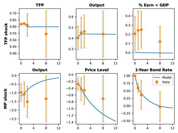
Figure 1: Model-implied impulse responses (thin curves) and corresponding empirical estimates (circles), with respect to a one-standard-deviation TFP shock (top row) or a monetary policy shock that raises the bond rate by 1 percentage point on impact (bottom row). Figure titles: response variables (“% Earn < GDP”: fraction of people earning less than 2/3 of per capita GDP). Vertical axis units: percentage points. Horizontal axis units: quarters. Vertical error bars: (shifted) 90% confidence intervals for the differences between the empirical and model-implied moments (not confidence intervals for the empirical moments themselves).

Figure 1 compares the model-implied and empirical impulse responses, at the parameter estimates discussed in the previous paragraph. We see that the model-implied impulse responses of output to a monetary shock are too small in magnitude relative to the data at the 2- and 8-quarter horizons, while the opposite is true for the responses of the price level with respect a monetary shock. Moreover, the model fails to generate nontrivial dynamics in the fraction of low-wage earners in response to a TFP shock. To test whether these disparities are too large to be explained by statistical noise, we conduct the over-identification test proposed in Section 4.2. The vertical error bars in Figure 1 show the 90% confidence intervals for the differences between model-implied and empirical moments, centered at the empirical moments for visual convenience. Three of the model-implied impulse responses for the fraction of low-wage earners fall outside their respective intervals, though only marginally so. While this points to misspecification of either the structural model or the reduced-form VAR models used to generate the empirical impulse responses, we note that the joint test of the validity of all $p=23$ moments does not reject at the 10% level.

The efficient (one-step) parameter estimates in the bottom row of Table 2 demonstrate the benefit of optimally weighting the moments as described in Section 3.2. In particular, the t-statistic for the slope of the New Keynesian Phillips curve increases to 2.32, from 1.10 previously. Thus, our limited-information approach yields informative inference about a parameter that is often viewed as difficult to pin down in the data (Mavroeidis et al., 2014). More generally, the efficient standard errors in the bottom row of Table 2 are 6–26% smaller than the non-efficient ones in the top row.

6 Conclusion

We computed simple, sharp, and informative upper bounds on the standard errors of structural parameter estimates when the correlation structure of the matched empirical moments is not fully known. In addition, we proposed an efficient moment weighting procedure in the over-identified case, as well as valid tests of parameter restrictions and over-identifying restrictions. The required inputs are minimal: Other than being able to evaluate the mapping from structural parameters to model-implied moments (at least numerically), we just need the empirical moment estimates and their individual standard errors. Our procedures are computationally tractable even in settings with many moments and/or parameters. A code suite is available online (see Footnote 1).

We believe our limited-information approach is useful for applied researchers who match their models to moments obtained from several different data sources, estimation methods, or previous papers. Our methods obviate the need to estimate the correlation structure across the various moments, which is sometimes difficult or impossible. Even when the moment correlation structure is in principle estimable, our methods may be helpful, since marginal standard errors for individual moments are typically much easier to obtain from standard econometric software than it is to figure out the joint distribution of all moments, as illustrated in our empirical applications. Moreover, the limited-information procedures can be used to gauge whether it is worthwhile to expend the additional effort required for full-information analysis.

Appendix A Appendix

A.1 Technical lemmas and proofs

Here we state and prove a technical lemma referred to in Section 3.2, and we provide the proofs of Propositions 1 and 2.

Lemma 2.

Assume $p,k\in\mathbb{N}$ and $p>k$. Let $\lambda\in\mathbb{R}^{k}$, and let $G\in\mathbb{R}^{p\times k}$ have full column rank. Let $G^{\perp}$ denote any $p\times(p-k)$ matrix with full column rank such that $G^{\prime}G^{\perp}=0_{k\times(p-k)}$. Let $\mathcal{S}_{p}$ denote the set of $p\times p$ symmetric positive semidefinite matrices $W$ such that $G^{\prime}WG$ is nonsingular. Then

$$\left\{WG(G^{\prime}WG)^{-1}\lambda\colon W\in\mathcal{S}_{p}\right\}=\left\{x\colon x\in\mathbb{R}^{p},\;G^{\prime}x=\lambda\right\}=\left\{G(G^{\prime}G)^{-1}\lambda+G^{\perp}z\colon z\in\mathbb{R}^{p-k}\right\}.$$

Proof.

We first show that

$$\left\{G(G^{\prime}G)^{-1}\lambda+G^{\perp}z\colon z\in\mathbb{R}^{p-k}\right\}\subset\left\{WG(G^{\prime}WG)^{-1}\lambda\colon W\in\mathcal{S}_{p}\right\}.$$ (11)

Pick any $z\in\mathbb{R}^{p-k}$, and define

$$W(z)\equiv(G,G^{\perp})\left(\begin{array}[]{cc}I_{k}&\tilde{\lambda}z^{\prime}\\ z\tilde{\lambda}^{\prime}&\delta I_{p-k}\end{array}\right)\left(\begin{array}[]{c}G^{\prime}\\ G^{\perp\prime}\end{array}\right),\quad\tilde{\lambda}\equiv\frac{1}{\lambda^{\prime}(G^{\prime}G)^{-1}\lambda}\lambda,$$

where $\delta>0$ is arbitrary but chosen large enough so that $W(z)$ is positive semidefinite. Then

$$W(z)G=(G,G^{\perp})\left(\begin{array}[]{cc}I_{k}&\tilde{\lambda}z^{\prime}\\ z\tilde{\lambda}^{\prime}&\delta I_{p-k}\end{array}\right)\left(\begin{array}[]{c}G^{\prime}G\\ 0_{(p-k)\times k}\end{array}\right)=(G+G^{\perp}z\tilde{\lambda}^{\prime})G^{\prime}G.$$

Hence,

$$G^{\prime}W(z)G=(G^{\prime}G)^{2},$$

implying

$$W(z)G(G^{\prime}W(z)G)^{-1}\lambda =(G+G^{\perp}z\tilde{\lambda}^{\prime})(G^{\prime}G)^{-1}\lambda=G(G^{\prime}G)^{-1}\lambda+G^{\perp}z,$$

and thus the statement (11) holds.

Now pick any $W\in\mathcal{S}_{p}$. Then $x=WG(G^{\prime}WG)^{-1}\lambda$ satisfies $G^{\prime}x=\lambda$. This shows that

$$\left\{WG(G^{\prime}WG)^{-1}\lambda\colon W\in\mathcal{S}_{p}\right\}\subset\left\{x\colon x\in\mathbb{R}^{p},\;G^{\prime}x=\lambda\right\}.$$ (12)

Finally, choose any $x\in\mathbb{R}^{p}$ satisfying $G^{\prime}x=\lambda$. Since the columns of $G$ and $G^{\perp}$ are (jointly) linearly independent, there exist $y\in\mathbb{R}^{k}$ and $z\in\mathbb{R}^{p-k}$ such that $x=Gy+G^{\perp}z$. Note that $\lambda=G^{\prime}x=G^{\prime}Gy$, so necessarily $y=(G^{\prime}G)^{-1}\lambda$. We have thus shown that

$$\left\{x\colon x\in\mathbb{R}^{p},\;G^{\prime}x=\lambda\right\}\subset\left\{G(G^{\prime}G)^{-1}\lambda+G^{\perp}z\colon z\in\mathbb{R}^{p-k}\right\}.$$ (13)

The set inclusions (11)–(13) together imply the statement of the lemma. ∎

Proof of Proposition 1.

It is standard to show that (3) holds under Assumption 1 (Newey & McFadden, 1994). Moreover,

$$\sqrt{n}\,\widehat{\text{se}}(\hat{x})\stackrel{{\scriptstyle p}}{{\to}}\sum_{j=1}^{p}V_{jj}^{1/2}|x_{j}|=\max_{\tilde{V}\in\mathcal{S}(\operatorname*{diag}(V))}\sqrt{x^{\prime}\tilde{V}x},$$

where the equality uses Lemma 1 in Section 3.1, $\operatorname*{diag}(V)$ is the vector of diagonal elements of $V$, and we recall the notation $x=WG(G^{\prime}WG)^{-1}\lambda$. Hence, letting $Z$ denote a standard normal random variable, we have

$$\lim_{n\to\infty}P(r(\theta_{0})\in\widehat{\text{CI}}) =\lim_{n\to\infty}P\left(\sqrt{n}|r(\hat{\theta})-r(\theta_{0})|\leq\Phi^{-1}(1-\alpha/2)\times\sqrt{n}\,\widehat{\text{se}}(\hat{x})\right)$$

$$=P\left(\sqrt{x^{\prime}Vx}\times|Z|\leq\Phi^{-1}(1-\alpha/2)\times\max_{\tilde{V}\in\mathcal{S}(\operatorname*{diag}(V))}\sqrt{x^{\prime}\tilde{V}x}\right)$$

$$\geq P\left(|Z|\leq\Phi^{-1}(1-\alpha/2)\right)$$

$$=1-\alpha.\qed$$

Proof of Proposition 2.

Under the null hypothesis,

$$\sqrt{n}r(\hat{\theta})\stackrel{{\scriptstyle d}}{{\to}}\lambda^{\prime}(G^{\prime}WG)^{-1}G^{\prime}WV^{1/2}Z,$$

where $V^{1/2}V^{1/2\prime}=V$, and $Z=(Z_{1},\dots,Z_{p})^{\prime}\sim N(0_{p\times 1},I_{p})$. The asymptotic null distribution of the test statistic $\hat{\mathscr{T}}$ is therefore a Gaussian quadratic form:

$$n\hat{\mathscr{T}}\stackrel{{\scriptstyle d}}{{\to}}Z^{\prime}QZ,\quad Q\equiv V^{1/2\prime}WG(G^{\prime}WG)^{-1}\lambda S\lambda^{\prime}(G^{\prime}WG)^{-1}G^{\prime}WV^{1/2}.$$

Székely & Bakirov (2003) prove that

$$P(Z^{\prime}QZ\leq\operatorname*{trace}(Q)\times\tau)\geq P(Z_{1}^{2}\leq\tau)$$ (14)

for any $p\times p$ symmetric positive semidefinite (non-null) matrix $Q$ and any $\tau>1.5365$. Since $(\Phi^{-1}(1-\alpha/2))^{2}>1.5365$ for $\alpha\leq 0.215$, it follows that, under the null,

$$P(\hat{\mathscr{T}}\leq\text{cv}_{n}) \geq P\left(n\hat{\mathscr{T}}\leq\operatorname*{trace}(Q)\times(\Phi^{-1}(1-\alpha/2))^{2}\right)$$

$$\to P\left(Z^{\prime}QZ\leq\operatorname*{trace}(Q)\times(\Phi^{-1}(1-\alpha/2))^{2}\right)$$

$$\geq P\left(Z_{1}^{2}\leq(\Phi^{-1}(1-\alpha/2))^{2}\right)$$

$$=1-\alpha.\qed$$

A.2 Simulated moments

We here argue that Proposition 1 can be extended to a setting where the model-implied moment function $h(\cdot)$ is not available analytically and we therefore resort to stochastic simulation to approximate it. The main requirement is that the number of simulation draws $M$ is sufficiently large relative to the empirical sample size $n$.

Let $\hat{h}_{M}(\cdot)$ denote the approximation of $h(\cdot)$ computed from $M$ simulation draws. For example, if we are matching simple moments of the form $h(\theta)=E[\tilde{h}(\theta,\zeta)]$, where $\tilde{h}(\cdot,\cdot)$ is a deterministic function and $\zeta$ is a random vector (e.g., the shocks in the structural model), then we can set $\hat{h}_{M}(\theta)=\frac{1}{M}\sum_{s=1}^{M}\tilde{h}(\theta,\zeta_{s})$, where $\zeta_{1},\dots,\zeta_{M}$ are draws from the distribution of $\zeta$. The minimum distance estimator $\hat{\theta}$ is defined as in (2), but with $\hat{h}_{M}(\cdot)$ in place of $h(\cdot)$. The worst-case standard errors are computed as in (5), except that we leave the estimator $\hat{G}=\hat{G}_{M}$ of $G=\frac{\partial h(\theta_{0})}{\partial\theta^{\prime}}$ unspecified for now (we return to this choice below).

Proposition 3.

Impose Assumption 1 and $\max_{j}|x_{j}|V_{jj}>0$. Assume further that as $n\to\infty$, we have $M\to\infty$, $n/M\to 0$, $\hat{G}_{M}\stackrel{{\scriptstyle p}}{{\to}}G$, and $\sup_{\theta\colon\|\theta-\theta_{0}\|\leq\delta_{M}}\sqrt{M}\|\hat{h}_{M}(\theta)-h(\theta)\|=O_{p}(1)$ for any sequence satisfying $\delta_{M}\to 0$. Then the conclusions of Proposition 1 apply.

Proof.

Upon inspection of the proof of Proposition 1, it suffices to show that (3) holds. We appeal to Theorem 7.2 in Newey & McFadden (1994), where, in their notation, $\hat{g}_{n}(\theta)=\hat{h}_{M}(\theta)-\hat{\mu}$ and $g_{0}(\theta)=h(\theta)-h(\theta_{0})$. The first three conditions of this theorem hold by Assumption 1(iii)–(vi). The fourth condition holds by Assumption 1(i) and $\sqrt{n}[\hat{h}_{M}(\theta_{0})-h(\theta_{0})]=\sqrt{n/M}\times\sqrt{M}[\hat{h}_{M}(\theta_{0})-h(\theta_{0})]=o(1)\times O_{p}(1)$. Finally, the fifth condition follows from

$$\sup_{\theta\colon\|\theta-\theta_{0}\|\leq\delta_{M}}\sqrt{n}\|\hat{g}_{n}(\theta)-\hat{g}_{n}(\theta_{0})-g_{0}(\theta)\| =\sup_{\theta\colon\|\theta-\theta_{0}\|\leq\delta_{M}}\sqrt{n}\|\hat{h}_{M}(\theta)-\hat{h}_{M}(\theta_{0})-[h(\theta)-h(\theta_{0})]\|$$

$$\leq 2\sqrt{n/M}\times\sup_{\theta\colon\|\theta-\theta_{0}\|\leq\delta_{M}}\sqrt{M}\|\hat{h}_{M}(\theta)-h(\theta)\|$$

$$=o(1)\times O_{p}(1).\qed$$

Remarks.

1. The key assumption is that the number of simulation draws $M$ is large relative to the empirical sample size $n$, in the sense $n/M\to 0$, so that the simulation noise in $\hat{h}_{M}(\cdot)$ is asymptotically negligible relative to the statistical noise in $\hat{\mu}$. In practice, we recommend that researchers choose $M$ sufficiently large so that the simulation noise in the moment estimates $\hat{h}_{M}(\hat{\theta})$ is orders of magnitude smaller than the empirical moment standard errors $\hat{\sigma}_{j}$.

2. The uniform tightness assumption $\sup_{\theta\colon\|\theta-\theta_{0}\|\leq\delta_{M}}\sqrt{M}\|\hat{h}_{M}(\theta)-h(\theta)\|=O_{p}(1)$ strengthens pointwise $\sqrt{M}$-consistency of $\hat{h}_{M}(\theta)$ (which usually follows straight-forwardly from a central limit theorem) to uniform $\sqrt{M}$-consistency for all $\theta$ in a neighborhood of $\theta_{0}$.

3. Under alternative asymptotics where $M$ is proportional to $n$, the worst-case standard error formula (5) would need to take into account the simulation noise, and the uniform tightness assumption would need to be strengthened to stochastic equicontinuity as in Newey & McFadden (1994, Theorem 7.2).

4. Consider again the special case with $h(\theta)=E[\tilde{h}(\theta,\zeta)]$ and $\hat{h}_{M}(\theta)=\frac{1}{M}\sum_{s=1}^{M}\tilde{h}(\theta,\zeta_{s})$, where we now assume that the draws $\{\zeta_{s}\}_{s=1}^{M}$ are strictly stationary across $s$. Then uniform tightness is implied by $\sum_{\ell=-\infty}^{\infty}\|\operatorname*{Cov}(\tilde{h}(\theta,\zeta_{s}),\tilde{h}(\theta,\zeta_{s-\ell}))\|$ being uniformly bounded for all $\theta$ in a neighborhood of $\theta_{0}$ (this follows from Chebyshev’s inequality). Notice that these conditions allow the simulated moments $\hat{h}_{M}(\theta)$ to be computed either by averaging across time (in a single simulated economy) or across independent simulated economies.

5. The only assumption required of the estimated Jacobian matrix $\hat{G}_{M}$ is consistency. Newey & McFadden (1994, Section 7.3) and Hong et al. (2015) discuss generic finite-difference derivative estimators based on simulation draws, and they provide assumptions ensuring consistency.

A.3 Details of extensions

Here we provide further details on the cases discussed in Section 3.3 where additional knowledge about the moment covariance matrix is available.

General constraint set.

Consider a general constraint set $\tilde{\mathcal{S}}$ defined by linear equality or inequality restrictions, as well as the positive semidefiniteness constraint. In the over-identified case $p>k$, the worst-case efficient weight matrix $W$ can be computed through two nested convex/concave optimization problems:

$$\min_{W\in\mathcal{S}_{p}}\max_{\tilde{V}\in\tilde{\mathcal{S}}}\,x(W)^{\prime}\tilde{V}x(W)=\min_{z\in\mathbb{R}^{p-k}}\max_{\tilde{V}\in\tilde{\mathcal{S}}}\,\{G(G^{\prime}G)^{-1}\lambda+G^{\perp}z\}^{\prime}\tilde{V}\{G(G^{\prime}G)^{-1}\lambda+G^{\perp}z\},$$ (15)

where $\mathcal{S}_{p}$, $x(W)$, and $G^{\perp}$ were defined in Section 3.2, and the equality follows from Lemma 2 in Section A.1. The inner maximization in (15) is a concave semidefinite program, as discussed in Section 3.3. The outer minimization is an unconstrained convex program since the objective function is a pointwise maximum of convex functions in $z$. The nested optimizations in (15) may be neither strictly convex nor differentiable, but for our purposes it suffices to use convex optimization algorithms that return any arbitrary local minimum $z^{*}$ (which is necessarily also a global minimum). Once an optimal $z^{*}$ has been computed, a corresponding optimal weight matrix is given by the matrix $W(z^{*})$ defined in the proof of Lemma 2 in Section A.1.

To conduct joint hypothesis tests as in Section 4, we can simply replace the constraint set in the critical value computation (9) with $\tilde{\mathcal{S}}$.

Special case: Knowledge of the block diagonal.

Suppose we know the block diagonal of $V$, while all other elements are unrestricted. That is, suppose the constraint set $\tilde{\mathcal{S}}$ is given by all symmetric positive semidefinite matrices of the form

$$V=\left(\begin{array}[]{ccccc}V_{(1)}&?&?&\dots&?\\ ?&V_{(2)}&?&\dots&?\\ \vdots&&\ddots&&\vdots\\ \vdots&&&\ddots&\vdots\\ ?&?&\dots&?&V_{(J)}\end{array}\right),$$ (16)

where $V_{(j)}$ are known (or consistently estimable) square symmetric matrices (possibly of different dimensions) for $j=1,\dots,J$. Partition the vectors $x$ and $\hat{\mu}$ conformably as $x=(x_{(1)}^{\prime},\dots,x_{(J)}^{\prime})^{\prime}$ and $\hat{\mu}=(\hat{\mu}_{(1)}^{\prime},\dots,\hat{\mu}_{(J)}^{\prime})^{\prime}$. The worst-case asymptotic standard deviation (8), for fixed $W$, is then given by

$$\sqrt{\max_{\tilde{V}\in\tilde{\mathcal{S}}}\,x^{\prime}\tilde{V}x}=\sum_{j=1}^{J}(x_{(j)}^{\prime}V_{(j)}x_{(j)})^{1/2}.$$ (17)

This follows from the same logic as in Lemma 1 in Section 3.1 once we recognize that the known block diagonal of $V$ implies that the marginal variance of $x_{(j)}^{\prime}\hat{\mu}_{(j)}$ is known for each $j=1,\dots,J$, but the correlations among these $J$ variables remain unrestricted. Specifically, the maximum (17) is achieved by $V=\operatorname*{Var}(\tilde{\mu})$, where the random vector $\tilde{\mu}=(\tilde{\mu}_{(1)}^{\prime},\dots,\tilde{\mu}_{(J)}^{\prime})^{\prime}$ has the following representation. Let $\eta=(\eta_{(1)}^{\prime},\dots,\eta_{(J)}^{\prime})^{\prime}$ have the covariance matrix (16), but with zeros instead of question marks. Let $\bar{\eta}$ be a scalar random variable with variance 1 that is uncorrelated with $\eta$. Then set $\tilde{\mu}_{(j)}\equiv\frac{1}{\sqrt{x_{(j)}^{\prime}V_{(j)}x_{(j)}}}V_{(j)}x_{(j)}\bar{\eta}+(I-\frac{1}{x_{(j)}^{\prime}V_{(j)}x_{(j)}}V_{(j)}x_{(j)}x_{(j)}^{\prime})\eta_{(j)}$, $j=1,\dots,J$.

In the over-identified case, the worst-case efficient weight matrix can be computed by substituting the formula (17) into the nested optimization (15) (with $x=G(G^{\prime}G)^{-1}\lambda+G^{\perp}z$).

A.4 Details of the price setting application and simulation study

Here we provide details of the data used for the empirical application in Section 5.1, and we conduct a simulation study calibrated to this application.

Data.

We use the “movement” data set for beer products (file name wber.csv) on the Chicago Booth website. We follow Alvarez et al. (2016) when cleaning the data. First, we keep only data for store #122. Second, we drop any observations with prices below 20 cents or above 25 dollars (the data was collected between the years 1989 and 1994). Third, we set any absolute price changes below one cent equal to zero. Fourth, we drop the largest 1% of absolute log price changes.

Price setting application: Reduced-form moment estimates
Moment Estimate Std. error Pairwise correlation $\times 1000$ $E[(\Delta p)^{2}]$ $E[(\Delta p)^{4}]$ $E[|\Delta p|]$ Frequency 0.293 2.338 0.000 0.000 0.000 $E[(\Delta p)^{2}]$ 0.027 0.233 0.939 0.966 $E[(\Delta p)^{4}]$ 0.001 0.019 0.831 $E[|\Delta p|]$ 0.145 0.754

Table 3: Reduced-form moment estimates and their standard errors: average weekly rate of nonzero price changes (Frequency), and moments $E[|\Delta p|^{j}]$, $j=1,2,4$ of absolute log price changes conditional on a nonzero change. “Pairwise correlation” columns: estimated pairwise correlations across the sample moments.

Table 3 shows the $p=4$ estimated reduced-form moments, their standard errors, and their estimated correlation matrix. The sample kurtosis (fourth moment divided by squared second moment) of log price changes equals 1.80. The zero correlation between the sample frequency of nonzero price changes (a binary outcome) and the sample moments of the price change magnitudes is mechanical. Our limited-information analysis here does not exploit this fact because we want to emulate what an applied researcher might do without thinking hard about the problem. However, the independence could be taken into account using the extensions described in Section 3.3.

Simulation study.

We apply the inference methods to data simulated from the Alvarez & Lippi (2014) model. The simulations treat the just-identified empirical parameter estimates (columns 1–3 in Table 1) as the truth, and we use a sample size of $n=\text{37,916}$ as in the real data. The binary price change indicators are drawn i.i.d. from a binomial distribution with the model-implied success probability (Alvarez & Lippi, 2014, Proposition 4). The magnitudes of the price changes are drawn from the model-implied density function (Alvarez & Lippi, 2014, Proposition 6). We use 10,000 Monte Carlo repetitions. The estimation and inference procedures are the same as the ones applied to the actual data (in particular, efficient estimates are computed using the one-step approach).

Monte Carlo simulation study
Just-identified specification Efficient specification # prod. Vol. Menu cost # prod. Vol. Menu cost Confidence interval coverage rate Full-info 94.5% 95.0% 94.7% 95.0% 95.2% 95.3% Independence 100.0% 95.0% 100.0% 100.0% 89.1% 100.0% Worst case 100.0% 99.4% 100.0% 100.0% 99.4% 100.0% Confidence interval average length Full-info 0.179 0.002 0.010 0.162 0.002 0.009 Independence 0.627 0.002 0.039 0.390 0.002 0.025 Worst case 0.878 0.003 0.059 0.571 0.003 0.041 RMSE relative to true parameter values Full-info 1.53% 0.59% 0.86% 1.37% 0.58% 0.76% Independence 1.53% 0.59% 0.86% 1.72% 0.59% 0.99% Worst case 1.53% 0.59% 0.86% 1.79% 0.59% 1.03% Rejection rate of over-identification test Full-info 5.01% Independence 0.00% Worst case 0.00% Rejection rate of joint test of true parameter values Full-info 4.79% Independence 7.54% Worst case 2.47%

Table 4: Simulation results based on the empirically calibrated Alvarez & Lippi (2014) model. The just-identified specification uses only three moments for estimation, while the efficient specification exploits all four moments. The rows correspond to full-information inference (exploits knowledge of $\hat{V}$), inference under independence (erroneously assumes that $\hat{V}$ is diagonal), and worst-case inference (exploits only diagonal of $\hat{V}$ without assuming off-diagonal elements are zero). Estimated parameters: number of products (# prod.), volatility of desired log price (Vol.), scaled menu cost (Menu cost). The over-identification test tests the validity of the fourth non-targeted moment. The joint test of the true parameters is a Wald test (Full-info or Independence) or the test proposed in Section 4.1 (Worst case). The nominal significance level is 5%.

Table 4 shows that the just-identified and efficient limited-information confidence intervals have coverage probabilities very nearly equal to or exceeding the nominal level of 95% for all three parameters. Though coverage is conservative, the table shows that the average length of the confidence intervals is not more than six times that of the corresponding full-information confidence intervals. This is consistent with the empirical standard errors reported in Section 5.1.

Table 4 also illustrates that the worst-case perspective is key to avoiding over-rejection in the face of limited information: Both the “efficient” t-test for the price volatility parameter and the joint Wald test of the true parameter values over-reject if we erroneously assume that all the empirical moments are independent of each other. In contrast, the limited-information and full-information t-tests and joint tests are correctly sized. The limited-information tests are conservative (as predicted by theory), though the joint test of parameter restrictions is only mildly conservative in this particular model.

Finally, Table 4 shows that the limited-information efficient point estimates have slightly higher root mean squared error (RMSE) than the efficient full-information estimates. It may seem surprising at first blush that the limited-information efficient estimates can have (marginally) higher RMSE than the just-identified estimates. This is because the limited-information efficient estimates are designed to have low variance under the worst-case correlation structure (i.e., perfect correlation of the moments), not under the true correlation structure that is unknown to the econometrician.

A.5 Details of the heterogeneous agent application

We here provide further details on the application in Section 5.2. Table 5 shows which impulse response moments are used to efficiently estimate the seven structural parameters, according to the moment selection procedure described in Section 3.2. The $p=23$ moments are shown along the rows, while the $k=7$ parameters are shown along the columns. A cell with an “x” indicates a non-zero efficient loading ($\hat{x}_{j}^{*}$ in the notation of Section 3.2), while empty cells indicate zero loadings.

Heterogeneous agent application: Efficient moment selection
Impulse response TFP Monetary Var. Shock Horiz. TR PC AR1 AR2 Std AR1 AR2 TFP TFP 0 x x x x x 1 x x x x 2 x x x x 8 Output TFP 0 x x x 1 2 8 Frac TFP 0 1 2 8 Output MP 0 x x x x 1 2 8 Price MP 0 x x 1 2 x 8 Bond MP 1 x x x x 2 8 x x

Table 5: Cells with an “x” indicate that the efficient estimate of the given parameter (along columns) attaches a non-zero weight to the given empirical moment (along rows). First three columns show the impulse response variable (“Var.”), shock, and quarterly horizon (“Horiz.”). Variable “Frac”: fraction of people earning less than 2/3 of GDP. Shock “MP”: monetary shock. See parameter abbreviations in Table 2.

References

- Altonji & Segal (1996) Altonji, J. G. & Segal, L. M. (1996). Small-Sample Bias in GMM Estimation of Covariance Structures. Journal of Business & Economic Statistics, 14(3), 353–366.
- Alvarez et al. (2016) Alvarez, F., Le Bihan, H., & Lippi, F. (2016). The Real Effects of Monetary Shocks in Sticky Price Models: A Sufficient Statistic Approach. American Economic Review, 106(10), 2817–2851.
- Alvarez & Lippi (2014) Alvarez, F. & Lippi, F. (2014). Price Setting With Menu Cost for Multiproduct Firms. Econometrica, 82(1), 89–135.
- Auclert et al. (2021) Auclert, A., Bardóczy, B., Rognlie, M., & Straub, L. (2021). Using the Sequence-Space Jacobian to Solve and Estimate Heterogeneous-Agent Models. Econometrica, 89(5), 2375–2408.
- Chang et al. (2023) Chang, M., Chen, X., & Schorfheide, F. (2023). Heterogeneity and Aggregate Fluctuations. Manuscript, University of Pennsylvania.
- DeJong & Dave (2011) DeJong, D. N. & Dave, C. (2011). Structural Macroeconometrics (2nd ed.). Princeton University Press.
- Driscoll & Kraay (1998) Driscoll, J. C. & Kraay, A. C. (1998). Consistent Covariance Matrix Estimation with Spatially Dependent Panel Data. Review of Economics and Statistics, 80(4), 549–560.
- Evans & Honkapohja (2005) Evans, G. W. & Honkapohja, S. (2005). An Interview with Thomas J. Sargent. Macroeconomic Dynamics, 9(4), 561–583.
- Georgescu et al. (2018) Georgescu, D. I., Higham, N. J., & Peters, G. W. (2018). Explicit solutions to correlation matrix completion problems, with an application to risk management and insurance. Royal Society Open Science, 5(3), 1–11.
- Hahn et al. (2020) Hahn, J., Kuersteiner, G., & Mazzocco, M. (2020). Estimation with Aggregate Shocks. Review of Economic Studies, 87(3), 1365–1398.
- Hahn et al. (2022a) Hahn, J., Kuersteiner, G., & Mazzocco, M. (2022a). Central Limit Theory for Combined Cross Section and Time Series With an Application to Aggregate Productivity Shocks. Econometric Theory. Forthcoming.
- Hahn et al. (2022b) Hahn, J., Kuersteiner, G., & Mazzocco, M. (2022b). Joint Time Series and Cross-Section Limit Theory under Mixingale Assumptions. Econometric Theory, 38(5), 942–958.
- Hansen & Heckman (1996) Hansen, L. & Heckman, J. (1996). The Empirical Foundations of Calibration. Journal of Economic Perspectives, 10(1), 87–104.
- Hong et al. (2015) Hong, H., Mahajan, A., & Nekipelov, D. (2015). Extremum estimation and numerical derivatives. Journal of Econometrics, 188(1), 250–263.
- Imbens (2002) Imbens, G. W. (2002). Generalized Method of Moments and Empirical Likelihood. Journal of Business & Economic Statistics, 20(4), 493–506.
- Imbens & Lancaster (1994) Imbens, G. W. & Lancaster, T. (1994). Combining Micro and Macro Data in Microeconometric Models. Review of Economic Studies, 61(4), 655–680.
- Koenker & Bassett (1978) Koenker, R. & Bassett, G. (1978). Regression Quantiles. Econometrica, 46(1), 33–50.
- Kydland & Prescott (1996) Kydland, F. E. & Prescott, E. C. (1996). The Computational Experiment: An Econometric Tool. Journal of Economic Perspectives, 10(1), 69–85.
- Liu & Plagborg-Møller (2023) Liu, L. & Plagborg-Møller, M. (2023). Full-information estimation of heterogeneous agent models using macro and micro data. Quantitative Economics, 14(1), 1–35.
- Mavroeidis et al. (2014) Mavroeidis, S., Plagborg-Møller, M., & Stock, J. H. (2014). Empirical Evidence on Inflation Expectations in the New Keynesian Phillips Curve. Journal of Economic Literature, 52(1), 124–188.
- McKay et al. (2016) McKay, A., Nakamura, E., & Steinsson, J. (2016). The Power of Forward Guidance Revisited. American Economic Review, 106(10), 3133–58.
- Miranda-Agrippino & Ricco (2021) Miranda-Agrippino, S. & Ricco, G. (2021). The Transmission of Monetary Policy Shocks. American Economic Journal: Macroeconomics, 13(3), 74–107.
- Mongey & Williams (2017) Mongey, S. & Williams, J. (2017). Firm dispersion and business cycles: Estimating aggregate shocks using panel data. Manuscript, New York University.
- Nakamura & Steinsson (2018) Nakamura, E. & Steinsson, J. (2018). Identification in Macroeconomics. Journal of Economic Perspectives, 32(3), 59–86.
- Newey & McFadden (1994) Newey, W. K. & McFadden, D. L. (1994). Large Sample Estimation and Hypothesis Testing. In R. F. Engle & D. L. McFadden (Eds.), Handbook of Econometrics, Volume IV chapter 36, (pp. 2111–2245). Elsevier.
- Székely & Bakirov (2003) Székely, G. J. & Bakirov, N. K. (2003). Extremal probabilities for Gaussian quadratic forms. Probability Theory and Related Fields, 126(2), 184–202.
- Winberry (2018) Winberry, T. (2018). A method for solving and estimating heterogeneous agent macro models. Quantitative Economics, 9(3), 1123–1151.