Asymptotic Properties of $\mathcal{S}$-$\mathcal{AB}$ Method with Diminishing Step-size

Abstract

The popular $\mathcal{AB}$/push-pull method for distributed optimization problem may unify much of the existing decentralized first-order methods based on gradient tracking technique. More recently, the stochastic gradient variant of $\mathcal{AB}$/Push-Pull method ($\mathcal{S}$-$\mathcal{AB}$) has been proposed, which achieves the linear rate of converging to a neighborhood of the global minimizer when the step-size is constant. This paper is devoted to the asymptotic properties of $\mathcal{S}$-$\mathcal{AB}$ with diminishing step-size. Specifically, under the condition that each local objective is smooth and the global objective is strongly-convex, we first present the boundedness of the iterates of $\mathcal{S}$-$\mathcal{AB}$ and then show that the iterates converge to the global minimizer with the rate $\mathcal{O}\left(1/k\right)$ in the mean square sense. Furthermore, the asymptotic normality of Polyak-Ruppert averaged $\mathcal{S}$-$\mathcal{AB}$ is obtained and applications on statistical inference are discussed. Finally, numerical tests are conducted to demonstrate the theoretic results.

I Introduction

Distributed optimization problem is to minimize a finite sum of functions over a network made up of multi agents, where each agent holds the local objective function and can communicate with its neighbors. Distributed optimization problem has many applications in large-scale machine learning [1], wireless networks [2], parameter estimation [3], to name a few. Over the last decades, numerous algorithms for distributed optimization problem have been developed. This includes (sub)gradient method [4, 5, 6, 7, 8, 9, 10], dual averaging method [11, 12], primal dual method [13, 14], gradient push method [15, 16, 17], gradient tracking method [18, 19, 20]. We refer to the survey [21] for the new development on distributed optimization.

Recently, Xin and Khan [22] and Pu et al. [23] propose the $\mathcal{AB}$/push-pull method, which is suitable for the cases that the communication network is directed. $\mathcal{AB}$/push-pull method utilizes a row stochastic matrix for mixing the decision variables and a column stochastic matrix for tracking the average gradients. Since $\mathcal{AB}$/push-pull method may unify much of the existing decentralized first-order methods based on gradient tracking technique [24], many works have been devoted to the development of $\mathcal{AB}$/push-pull method. Pu [25] introduces an adapted version of push-pull method which inherits the linear convergence property of push pull method under noiseless communication links and has more robust performance than push pull method under noisy information exchange. Xiong et al. [26] propose a novel quantized distributed gradient tracking method to improve communication efficiency further, which can be rewritten as an inexact version of $\mathcal{AB}$/push-pull method. Saadatniaki et al. [27] propose a variant of $\mathcal{AB}$/push-pull method with time-varying weight matrices and show that the proposed method converges linearly to the optimal solution when each local objective is smooth and the global objective is strongly-convex. Accelerate techniques have also been incorporated into $\mathcal{AB}$/push-pull method, Xin and Khan [28] employ the heavy-ball method to accelerate the $\mathcal{AB}$/push-pull method where the R-linear rate for strongly convex smooth objective has been obtained. Xin et al. [29] combine nesterov gradient method with $\mathcal{AB}$/push-pull method and show that the new method achieves robust numerical performance for both convex and strongly-convex objectives. Moreover, the extended versions of $\mathcal{AB}$/push-pull method have been used to solve resource allocation [30] and the distributed multi-cluster game [31].

More recently, stochastic gradient version of $\mathcal{AB}$/push-pull method ($\mathcal{S}$-$\mathcal{AB}$) has been proposed in [32, 18]. Xin et al. [32] focus on the case that the step-size is constant and show that the iterates of $\mathcal{S}$-$\mathcal{AB}$ converge linearly to a neighborhood of the global minimizer when agents’ cost functions are smooth and strongly-convex. Pu and Nedić [18] study the convergence properties of distributed stochastic gradient tracking method (DSGT), which can be regarded as a special $\mathcal{S}$-$\mathcal{AB}$ with doubly stochastic weight matrix. The authors show that DSGT converges to the global optimal solution with the optimal rate $\mathcal{O}(1/k)$ when the stepsize diminishes to zero. Motivated by [32, 18], this paper is devoted to developing $\mathcal{S}$-$\mathcal{AB}$ by studying the convergence properties when the step-size is diminishing. We focus on the convergence of the iterate of $\mathcal{S}$-$\mathcal{AB}$ in the mean square sense and its asymptotic normality. As far as we are concerned, the contributions of the paper can be summarized as follows.

• The optimal convergence rate of $\mathcal{S}$-$\mathcal{AB}$ in the mean square sense. We show that the iterates of $\mathcal{S}$-$\mathcal{AB}$ converge to the global optimal solution with the rate $\mathcal{O}(1/k)$ when each local objective is smooth and the global objective is strongly-convex, which arrives at the optimal rate of vanilla stochastic gradient decent algorithm with diminishing stepsize. Indeed, the convergence of stochastic approximation (SA) based methods for distributed stochastic optimization problem with diminishing step-size have been well studied [5, 13, 18, 15], where most of the results are based on the fact that the stochastic gradient noise is a martingale difference sequence. Note that agents’ accumulated stochastic gradient noises during gradient tracking steps form the autoregressive moving average processes [33]. The challenge for $\mathcal{S}$-$\mathcal{AB}$ is that the weighted average of the accumulated stochastic gradient noises is not a martingale difference sequence as the weight matrices are not doubly stochastic.

• The asymptotic normality of $\mathcal{S}$-$\mathcal{AB}$. We present that Polyak-Ruppert averaged $\mathcal{S}$-$\mathcal{AB}$ converges in distribution to a normal random vector for any agent by combining the convergence rate of $\mathcal{S}$-$\mathcal{AB}$ and results on asymptotic normality of SA based algorithm [33, Theorem 3.4.2]. The asymptotic normality of stochastic approximation based algorithms can be traced back to 1950s [34, 35]. For the asymptotic normality on distributed stochastic optimization problem, we refer to [5, 6, 13] for unconstrained problems and [36, 37] for constrained problems. Complement to the works mentioned above, the new result does not need the communication network to be undirected or weight matrix to be doubly stochastic.

• The estimator of the covariance matrix. A series of works [38, 39, 40] have focused on estimating the covariance matrix in the limit normal distribution of vanilla stochastic gradient decent algorithm. We extend the plug-in method [38] to estimate the covariance matrix for the normal distribution of $\mathcal{S}$-$\mathcal{AB}$, which paves the way for doing statistical inference. Moreover, numerical experiments are provided to support our theoretical analysis.

The rest of this paper is organized as follows. Section II introduces the distributed stochastic optimization problem model, the $\mathcal{S}$-$\mathcal{AB}$ method and presents some standard assumptions in distributed stochastic optimization problem. Section III focuses on the convergence rate and asymptotic normality of the $\mathcal{S}$-$\mathcal{AB}$ method. At last, numerical results are presented in Section IV to validate the theoretic results.

Throughout this paper, we use the following notations. $\mathbb{R}^{d}$ denotes the d-dimension Euclidean space endowed with norm $\|x\|=\sqrt{\langle x,x\rangle}$. Denote $\mathbf{1}:=(1~{}1\dots 1)^{\intercal}$, $\mathbf{0}:=(0~{}0\dots 0)^{\intercal}$ and whose dimension will be clear in the context. $\mathbf{I}_{d}\in\mathbb{R}^{d\times d}$ stands for the identity matrix. $\mathbf{A}\otimes\mathbf{B}$ denotes the Kronecker product of matrices $\mathbf{A}$ and $\mathbf{B}$. For a sequence of random vectors $\{\xi_{k}\}$ and a random vector $\xi$, $\xi_{k}\stackrel{{\scriptstyle d}}{{\rightarrow}}\xi$ represents the convergence in distribution, $\mathrm{Cov}$($\xi$) denotes the covariance matrix of random vector $\xi$. $N\left(\mu,\Sigma\right)$ is the normal distribution with mean $\mu$ and covariance matrix $\Sigma$. For any sequences $\{a_{k}\}$ and $\{b_{k}\}$ of positive number, $a_{k}=\mathcal{O}(b_{k})$ if there exists $c>0$ such that $a_{k}\leq cb_{k}$.

II Problem formulation and $\mathcal{S}$-$\mathcal{AB}$ method

In this paper, we consider the following distributed stochastic optimization (DSO) problem

$$\min_{x\in\mathbb{R}^{d}}~{}f(x)=\sum_{j=1}^{n}f_{j}(x),$$ (1)

where $f_{j}(x):=\mathbb{E}[g_{j}(x;\zeta_{j})]$ denotes the cost of agent $j$, $g_{j}(x;\zeta_{j}):\mathbb{R}^{d}\times\Omega\rightarrow\mathbb{R}$ is the measure function, $\zeta_{j}$ is a random variable defined on a probability space $(\Omega,\mathcal{F},\mathrm{P})$ and $\mathbb{E}[\cdot]$ denotes the expectation with respect to probability $\mathrm{P}$. For DSO (LABEL:problem_model), the communication relationship between agents is characterized by a directed graph, $\mathcal{G}=\left(\mathcal{V},\mathcal{E}\right)$, where $\mathcal{V}=\{1,2,...,n\}$ is the node set with node $i$ representing agent $i$ and $\mathcal{E}\subseteq\mathcal{V}\times\mathcal{V}$ denotes the edge set with edge $(j,i)$ representing agent $i$ can receive information from agent $j$.

The $\mathcal{S}$-$\mathcal{AB}$ method in [32] reads as follows.

Algorithm 1 $\mathcal{S}$-$\mathcal{AB}$: At each node $i\in\mathcal{V}=\{1,2,...,n\}$

Require: initial value $x_{i,0}\in\mathbb{R}^{d}$, $y_{i,0}=\nabla g_{i}(x_{i,0},\zeta_{i,0})$, weight matrices $\mathbf{A}=\{a_{ij}\}$ and $\mathbf{B}=\{b_{ij}\}$.

• For $k=1,2,\cdots$ do

• State update:

  $$x_{i,k+1}=\sum_{j=1}^{n}a_{ij}x_{j,k}-\alpha_{k}y_{i,k}.$$ (2)

• Gradient tracking update:

  $$y_{i,k+1}=\sum_{j=1}^{n}b_{ij}y_{j,k}+\nabla g_{i}(x_{i,k+1},\zeta_{i,k+1})-\nabla g_{i}(x_{i,k},\zeta_{i,k}),$$

  where $\zeta_{i,0},\zeta_{i,1},\cdots$ is independent and identically distributed sample of $\zeta_{i}$.

• end for

Throughout our analysis in the paper, we make the following two assumptions on the objective function and weight matrices $\mathbf{A}$ and $\mathbf{B}$.

Assumption 1 (objective function).

• Function $f(x)$ is differentiable and $\mu$-strongly convex in $x$, that is

  $$f(y)\geq f(x)+\langle\nabla f(x),y-x\rangle+\frac{\mu}{2}\|x-y\|^{2},\quad\forall x,y\in\mathbb{R}^{d}.$$

• Let $x^{*}$ be an optimal solution. There exists a constant $c>0$ such that

  $$\|\nabla f(x)-\nabla^{2}f(x^{*})\left(x-x^{*}\right)\|\leq c\|x-x^{*}\|^{2},\quad\forall x\in\mathbb{R}^{n}.$$

• For any $i\in\mathcal{V}$, function $g_{i}(x,\zeta_{i})$ is differentiable and there exist constants $p>2$, $U_{1}>0$ such that

  $$\mathbb{E}\left[\|\nabla g_{i}(x;\zeta_{i})-\nabla f_{i}(x)\|^{p}\right]\leq U_{1}^{p/2},$$

  $$\|\nabla g_{i}(x;\zeta_{i})-\nabla g_{i}(y;\zeta_{i})\|\leq L_{i}(\zeta_{i})\|x-y\|,\quad\forall x,y\in\mathbb{R}^{d},$$

  where $L_{i}(\zeta_{i})$ is a positive random variable and satisfies $\mathbb{E}[L_{i}^{p}(\zeta_{i})]<\infty$.

Assumption 1 (i)- (ii) are standard conditions on objective and have been well used to study the asymptotic properties of SA based method [41, 42]. In Assumption 1 (iii), the constant $p=2$ is sufficient to investigate the convergence rate of $\mathcal{S}$-$\mathcal{AB}$ as [32, 24], while $p>2$ is needed for the asymptotic normality of $\mathcal{S}$-$\mathcal{AB}$. Define $L:=\max_{1\leq i\leq n}\sqrt{\mathbb{E}[L_{i}^{2}(\zeta_{i})]}$. Then for any $x,y\in\mathbb{R}^{d}$, we have

$$\|\nabla f_{i}(x)-\nabla f_{i}(y)\|^{2} \leq L^{2}\|x-y\|^{2}$$ (3)

and

$$\left\|\frac{1}{n}\sum_{j=1}^{n}\nabla f_{j}(x_{i})-\frac{1}{n}\nabla f(y)\right\|^{2} =\left\|\frac{1}{n}\sum_{j=1}^{n}\left(\nabla f_{j}(x_{i})-\nabla f_{j}(y)\right)\right\|^{2}$$

$$\leq\frac{1}{n}\sum_{j=1}^{n}\left\|\nabla f_{j}(x_{i})-\nabla f_{j}(y)\right\|^{2}$$

$$\leq\frac{L^{2}}{n}\sum_{j=1}^{n}\|x_{i}-y\|^{2}.$$ (4)

Assumption 2 (weight matrices and networks).

Let $\mathcal{G}_{A}=\left(\mathcal{V},\mathcal{E}_{\mathbf{A}}\right)$ and $\mathcal{G}_{B^{\intercal}}=\left(\mathcal{V},\mathcal{E}_{\mathbf{B}^{\intercal}}\right)$ be graphs induced by matrices $\mathbf{A}$ and $\mathbf{B}^{\intercal}$ respectively. Suppose that

• The matrix $\mathbf{A}\in\mathbb{R}^{n\times n}$ is nonnegative row stochastic and $\mathbf{B}\in\mathbb{R}^{n\times n}$ is nonnegative column stochastic, i.e., $\mathbf{A}\mathbf{1}=\mathbf{1}$ and $\mathbf{1}^{\intercal}\mathbf{B}=\mathbf{1}^{\intercal}$. In addition, the diagonal entries of $\mathbf{A}$ and $\mathbf{B}$ are positive, i.e., $\mathbf{A}_{ii}>0$ and $\mathbf{B}_{ii}>0$ for all $i\in\mathcal{V}$.

• The graphs $\mathcal{G}_{A}$ and $\mathcal{G}_{B^{\intercal}}$ each contain at least one spanning tree. Moreover, there exists at least one node that is a root of spanning trees for both $\mathcal{G}_{A}$ and $\mathcal{G}_{B^{\intercal}}$, i.e. $\mathcal{R}_{A}\cap\mathcal{R}_{B^{\intercal}}\neq\emptyset$, where $\mathcal{R}_{A}$ ( $\mathcal{R}_{B^{\intercal}}$) is the set of roots of all possible spanning trees in the graph $\mathcal{G}_{A}$ ( $\mathcal{G}_{B^{\intercal}}$).

As commented in [43], Assumption 2 is weaker than requiring that both $\mathcal{G}_{A}$ and $\mathcal{G}_{B^{\intercal}}$ are strongly connected. Building on consensus with non-doubly stochastic matrices, the scheme of $\mathcal{AB}$/push-pull method has been applied on reinforce learning [44] and economic dispatch problem [45]. Under Assumption 2, the matrix $\mathbf{A}$ has a nonnegative left eigenvector $u^{\intercal}$ (w.r.t. eigenvalue 1) with $u^{\intercal}\mathbf{1}=n$, and the matrix $\mathbf{B}$ has a nonnegative right eigenvector $v$ (w.r.t. eigenvalue 1) with $\mathbf{1}^{T}v=n$. Moreover, $u^{\intercal}v>0$.

For easy of presentation, we rewrite Algorithm 1 in a compact form:

$$x_{k+1}=\tilde{\mathbf{A}}x_{k}-\alpha_{k}y_{k},$$ (5)

$$y_{k+1}=\tilde{\mathbf{B}}y_{k}+\nabla G_{k+1}-\nabla G_{k},$$

where $\tilde{\mathbf{A}}:=\mathbf{A}\otimes\mathbf{I}_{d},~{}\tilde{\mathbf{B}}:=\mathbf{B}\otimes\mathbf{I}_{d}$, the vectors $x_{k}$, $y_{k}$ and $\nabla G_{k}$ concatenate all $x_{i,k}$’s, $y_{i,k}$’s and $\nabla g_{i}(x_{i,k},\zeta_{i,k})$’s respectively.

III The convergence rate and asymptotic normality

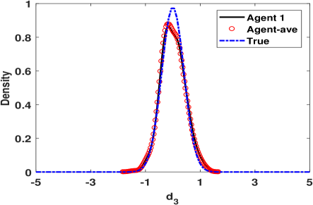
In this section, we study the convergence rate and asymptotic normality of $\mathcal{S}$-$\mathcal{AB}$ method. As commented in the introduction, the convergence rate of $\mathcal{S}$-$\mathcal{AB}$ has been discussed in [32, 18]. We focus on the rate of $x_{i,k}\to x^{*}$ rather than $x_{i,k}$ converging into a neighbor of $x^{*}$ [32]. Moreover, different from [18], the weighted average of the accumulated noises among agents can not form the martingale difference sequence as weight matrices $\mathbf{A}$ and $\mathbf{B}$ are not doubly stochastic.

We first study the convergence rate of iterates of $\mathcal{S}$-$\mathcal{AB}$ in the mean square sense. The following technical Lemma is an extension of [5, Lemma 3], which plays a key role in studying the stability and agreement of $\mathcal{S}$-$\mathcal{AB}$ method.

Lemma 1.

Suppose that positive sequences $\{\gamma_{k}\}$, $\{\rho_{k}\}$, $\{\phi_{k}\}$ satisfy

• $\{\gamma_{k}\}$, $\{\rho_{k}\}$ are $[0,1]$-valued sequences such that $\sum_{k=0}^{\infty}\gamma_{k}^{2}<\infty$, $\limsup_{k\rightarrow\infty}\frac{\gamma_{k}}{\gamma_{k+1}}=1$.

• $$\limsup_{k\rightarrow\infty}\left(\gamma_{k}\sqrt{\phi_{k}}+\frac{\phi_{k-1}}{\phi_{k}}\right)<\infty,\quad\sum_{k=0}^{\infty}\phi_{k}^{-1}<\infty,$$

  $$\liminf_{k\rightarrow\infty}\left(\gamma_{k}\sqrt{\phi_{k}}\right)^{-1}\left(\frac{\phi_{k-1}}{\phi_{k}}-\rho_{k}\right)>0.$$

If for scalars $M>0$ and $1>\rho>0$, sequences $\{u_{k}\},~{}\{v_{k}\}$ satisfy that for $k\geq k_{0}$,

$$u_{k+1} \leq\rho_{k}u_{k}+M\gamma_{k}\sqrt{u_{k}(1+u_{k}+v_{k})}$$ (6)

$$\quad+M\gamma_{k}\left(\gamma_{k}+\sum_{t=k_{0}}^{k}\gamma_{t}\rho^{k-t}u_{t}+\sum_{t=k_{0}}^{k}\gamma_{t}\rho^{k-t}v_{t}\right),$$

$$v_{k+1} \leq v_{k}+Mu_{k}+M\gamma_{k}\sqrt{u_{k}(1+u_{k}+v_{k})}$$ (7)

$$+M\gamma_{k}\left(\gamma_{k}+\sum_{t=k_{0}}^{k}\gamma_{t}\rho^{k-t}u_{t}+\sum_{t=k_{0}}^{k}\gamma_{t}\rho^{k-t}v_{t}\right),$$

then

$$\sup_{k}v_{k}<\infty,\quad\limsup_{k\rightarrow\infty}\phi_{k}u_{k}<\infty.$$

With Lemma 1 at hand, we are ready for presenting the stability and agreement of $\mathcal{S}$-$\mathcal{AB}$. To facilitate analysis, we define two auxiliary sequences $\{y_{k}^{{}^{\prime}}\}$ and $\{\xi_{k}\}$ as

$$y_{k+1}^{{}^{\prime}}=\tilde{\mathbf{B}}y_{k}^{{}^{\prime}}+\nabla F_{k+1}-\nabla F_{k},\quad y_{0}^{{}^{\prime}}=\nabla F_{0},$$ (8)

$$\xi_{k+1}=\tilde{\mathbf{B}}\xi_{k}+\epsilon_{k+1}-\epsilon_{k},\quad\xi_{0}=\epsilon_{0},$$ (9)

where vectors $\nabla F_{k}$ and $\epsilon_{k}$ concatenates all $\nabla f_{i}(x_{i,k})$’s and $\epsilon_{i,k}$’s respectively, $\epsilon_{i,k}:=\nabla g_{i}(x_{i,k};\zeta_{i,k})-\nabla f_{i}(x_{i,k})$.

Lemma 2.

Suppose that Assumptions 1 and 2 hold. Let step-size $\alpha_{k}=a/(k+b)^{\alpha}$, where $\alpha\in(1/2,1]$, positive scalars $a,b$ satisfy $\frac{a}{b^{\alpha}}\leq\min\{1,\frac{n}{u^{\intercal}vL}\}$, $L:=\max_{1\leq i\leq n}\sqrt{\mathbb{E}[L_{i}^{2}(\zeta_{i})]}$, where $u^{\intercal}$ and $v$ are the left eigenvector of $\mathbf{A}$ and the right eigenvector of $\mathbf{B}$ respectively (see Part II for the definitions). Then there exists a positive constant $U_{2}$ such that

$$\sup_{k}\mathbb{E}\left[\|\bar{x}_{k}-x^{*}\|^{2}\right]\leq U_{2},\quad\mathbb{E}\left[\|x_{k}-\mathbf{1}\otimes\bar{x}_{k}\|^{2}\right]\leq U_{2}\alpha_{k}^{2}$$

and

$$\mathbb{E}\left[\|y_{k}^{{}^{\prime}}-v\otimes\bar{y}_{k}^{{}^{\prime}}\|^{2}\right]\leq U_{2}\alpha_{k}^{2},$$

where

$$\bar{x}_{k}=\left(\frac{u^{\intercal}}{n}\otimes\mathbf{I}_{d}\right)x_{k},\quad\bar{y}_{k}^{{}^{\prime}}:=\left(\frac{\mathbf{1}^{\intercal}}{n}\otimes\mathbf{I}_{d}\right)y_{k}^{{}^{\prime}}.$$ (10)

Before presenting the proof of Lemma 2, we recall two vector norms [46, Lemma 3]

$$\|\mathbf{x}\|_{\mathbf{A}}:=\left\|\hat{\mathbf{A}}\mathbf{x}\right\|,\quad\|\mathbf{x}\|_{\mathbf{B}}:=\left\|\hat{\mathbf{B}}\mathbf{x}\right\|,\quad\forall x\in\mathbb{R}^{nd}$$

and their induced matrices norms

$$\left\|\mathbf{C}\right\|_{\mathbf{A}}:=\sup_{x\neq 0}\frac{\|\mathbf{C}x\|_{\mathbf{A}}}{\|x\|_{\mathbf{A}}},~{}\left\|\mathbf{C}\right\|_{\mathbf{B}}:=\sup_{x\neq 0}\frac{\|\mathbf{C}x\|_{\mathbf{B}}}{\|x\|_{\mathbf{B}}},~{}\forall\mathbf{C}\in\mathbb{R}^{nd\times nd},$$

where $\hat{\mathbf{A}},\hat{\mathbf{B}}\in\mathbb{R}^{nd\times nd}$ are some invertible matrices. These vector norms and their induced matrices norms have the following properties.

• $$\tau_{\mathbf{A}}:=\left\|\tilde{\mathbf{A}}-\frac{\mathbf{1}u^{\intercal}}{n}\otimes\mathbf{I}_{d}\right\|_{\mathbf{A}}<1,$$ (11)

  $$\tau_{\mathbf{B}}:=\left\|\tilde{\mathbf{B}}-\frac{v\mathbf{1}^{\intercal}}{n}\otimes\mathbf{I}_{d}\right\|_{\mathbf{B}}<1.$$ (12)

• $$\|\mathbf{C}x\|_{\mathbf{A}}\leq\|\mathbf{C}\|_{\mathbf{A}}\|x\|_{\mathbf{A}},\quad\|\mathbf{C}x\|_{\mathbf{B}}\leq\|\mathbf{C}\|_{\mathbf{B}}\|x\|_{\mathbf{B}}$$

  for any $\mathbf{C}\in\mathbb{R}^{nd\times nd},x\in\mathbb{R}^{nd}$.

• Let $\|\cdot\|_{*}$ and $\|\cdot\|_{**}$ be any two vector norms of $\|\cdot\|$, $\|\cdot\|_{\mathbf{A}}$ and $\|\cdot\|_{\mathbf{B}}$. There exists a constant $\overline{c}>1$ such that

  $$\|x\|_{*}\leq\overline{c}\|x\|_{**},\quad x\in\mathbb{R}^{nd}.$$ (13)

Proof.

We employ Lemma 1 to prove Lemma 2 and finish the proof by the following two steps: find relationships of $u_{k}$ and $v_{k}$ in the forms of (6) and (7) first, and then verify conditions (i)-(ii) of Lemma 1.

Step 1. By the definitions of $\bar{x}_{k}$, $y_{k}^{{}^{\prime}}$ and $\xi_{k+1}$ in (8)-(10), we have $y_{k}=y_{k}^{{}^{\prime}}+\xi_{k+1}$ and

$$\bar{x}_{k+1} =\left(\frac{u^{\intercal}}{n}\otimes\mathbf{I}_{d}\right)\tilde{\mathbf{A}}x_{k}-\alpha_{k}\left(\frac{u^{\intercal}}{n}\otimes\mathbf{I}_{d}\right)y_{k}$$ (14)

$$=\bar{x}_{k}-\alpha_{k}\left(\frac{u^{\intercal}}{n}\otimes\mathbf{I}_{d}\right)\left(y_{k}^{{}^{\prime}}+\xi_{k}\right)$$

$$=\bar{x}_{k}-\frac{u^{\intercal}v\alpha_{k}}{n^{2}}\nabla f(\bar{x}_{k})-\frac{u^{\intercal}v\alpha_{k}}{n}\left(\bar{y}^{{}^{\prime}}_{k}-\frac{1}{n}\nabla f(\bar{x}_{k})\right)$$

$$\quad-\alpha_{k}\left(\frac{u^{\intercal}}{n}\otimes\mathbf{I}_{d}\right)\left(y_{k}^{{}^{\prime}}-v\otimes\bar{y}^{{}^{\prime}}_{k}\right)-\alpha_{k}\left(\frac{u^{\intercal}}{n}\otimes\mathbf{I}_{d}\right)\xi_{k},$$

where the second equality follows from $u^{\intercal}\mathbf{A}=\mathbf{1}$. By the recursion (14),

$$\mathbb{E}\left[\|\bar{x}_{k+1}-x^{*}\|^{2}\right]$$ (15)

$$=\mathbb{E}\left[\left\|\bar{x}_{k}-x^{*}-\frac{u^{\intercal}v\alpha_{k}}{n^{2}}\nabla f(\bar{x}_{k})\right\|^{2}\right]$$

$$\quad+\alpha_{k}^{2}\mathbb{E}\left[\left\|\frac{u^{\intercal}v}{n}\left(\bar{y}^{{}^{\prime}}_{k}-\frac{1}{n}\nabla f(\bar{x}_{k})\right)-\left(\frac{u^{\intercal}}{n}\otimes\mathbf{I}_{d}\right)\left(y_{k}^{{}^{\prime}}-v\otimes\bar{y}^{{}^{\prime}}_{k}\right)\right.\right.$$

$$\quad\left.\left.-\left(\frac{u^{\intercal}}{n}\otimes\mathbf{I}_{d}\right)\xi_{k}\right\|^{2}\right]-2\mathbb{E}\left[\left\langle\bar{x}_{k}-x^{*}-\frac{u^{\intercal}v\alpha_{k}}{n^{2}}\nabla f(\bar{x}_{k}),\right.\right.$$

$$\quad\left.\left.\alpha_{k}\left(\frac{u^{\intercal}}{n}\otimes\mathbf{I}_{d}\right)\left(y_{k}^{{}^{\prime}}-\frac{v}{n}\otimes\nabla f(\bar{x}_{k})+\xi_{k}\right)\right\rangle\right]$$

$$\leq\mathbb{E}\left[\left\|\bar{x}_{k}-x^{*}-\frac{u^{\intercal}v\alpha_{k}}{n^{2}}\nabla f(\bar{x}_{k})\right\|^{2}\right]$$

$$\quad+3\alpha_{k}^{2}\left(\frac{u^{\intercal}v}{n}\right)^{2}\mathbb{E}\left[\left\|\bar{y}^{{}^{\prime}}_{k}-\frac{1}{n}\nabla f(\bar{x}_{k})\right\|^{2}\right]$$

$$\quad+\frac{3\alpha_{k}^{2}\|u\|^{2}\overline{c}^{2}}{n^{2}}\mathbb{E}\left[\left\|y_{k}^{{}^{\prime}}-v\otimes\bar{y}^{{}^{\prime}}_{k}\right\|_{\mathbf{B}}^{2}\right]+\frac{3\alpha_{k}^{2}\|u\|^{2}}{n^{2}}\mathbb{E}\left[\left\|\xi_{k}\right\|^{2}\right]$$

$$\quad-2\mathbb{E}\left[\left\langle\bar{x}_{k}-x^{*},\alpha_{k}\left(\frac{u^{\intercal}}{n}\otimes\mathbf{I}_{d}\right)\left(y_{k}^{{}^{\prime}}-\frac{v}{n}\otimes\nabla f(\bar{x}_{k})+\xi_{k}\right)\right\rangle\right]+$$

$$\quad 2\frac{u^{\intercal}v\alpha_{k}^{2}}{n^{2}}\mathbb{E}\left[\left\langle\nabla f(\bar{x}_{k}),\left(\frac{u^{\intercal}}{n}\otimes\mathbf{I}_{d}\right)\left(y_{k}^{{}^{\prime}}-\frac{v}{n}\otimes\nabla f(\bar{x}_{k})+\xi_{k}\right)\right\rangle\right].$$

By [47, Lemma 10], the first term on the right hand of (15)

$$\left\|\bar{x}_{k}-x^{*}-\frac{u^{\intercal}v\alpha_{k}}{n^{2}}\nabla f(\bar{x}_{k})\right\|^{2}\leq\left(1-\frac{u^{\intercal}v\mu\alpha_{k}}{n^{2}}\right)^{2}\left\|\bar{x}_{k}-x^{*}\right\|^{2}.$$ (16)

For the second term on the right hand side of (15),

$$3\alpha_{k}^{2}\left(\frac{u^{\intercal}v}{n}\right)^{2}\mathbb{E}\left[\left\|\bar{y}^{{}^{\prime}}_{k}-\frac{1}{n}\nabla f(\bar{x}_{k})\right\|^{2}\right]$$

$$=3\alpha_{k}^{2}\left(\frac{u^{\intercal}v}{n}\right)^{2}\mathbb{E}\left[\left\|\frac{1}{n}\sum_{i=1}^{n}\nabla f_{i}(x_{i,k})-\frac{1}{n}\nabla f(\bar{x}_{k})\right\|^{2}\right]$$

$$\leq 3\alpha_{k}^{2}\left(\frac{u^{\intercal}v}{n}\right)^{2}\frac{L^{2}\overline{c}^{2}}{n}\mathbb{E}\left[\left\|x_{k}-\mathbf{1}\otimes\bar{x}_{k}\right\|_{\mathbf{A}}^{2}\right],$$ (17)

where $\overline{c}$ is defined in (13), the equality follows from the fact $\bar{y}^{{}^{\prime}}_{k}=\frac{1}{n}\sum_{i=1}^{n}\nabla f_{i}(x_{i,k})$ and the inequality follows from (II). By Lemma 4 (i) in Appendix VI, the fourth term on the right hand of (15)

$$\frac{3\alpha_{k}^{2}\|u\|^{2}}{n^{2}}\mathbb{E}\left[\left\|\xi_{k}\right\|^{2}\right]\leq 3\alpha_{k}^{2}\frac{\|u\|^{2}c_{b}^{2}U_{1}}{n(1-\tau_{\mathbf{B}})^{2}},$$ (18)

where $c_{b}=\max\left\{\overline{c}^{2},\frac{\left\|\mathbf{B}-\mathbf{I}_{n}\right\|}{\tau_{\mathbf{B}}}\overline{c}^{2}\right\}$. Substitute (16)-(18) into (15),

$$\mathbb{E}\left[\|\bar{x}_{k+1}-x^{*}\|^{2}\right]$$ (19)

$$\leq\left(1-\frac{u^{\intercal}v\mu\alpha_{k}}{n^{2}}\right)^{2}\mathbb{E}\left[\left\|\bar{x}_{k}-x^{*}\right\|^{2}\right]+3\alpha_{k}^{2}\mathbb{E}\left[\left(\frac{u^{\intercal}v}{n}\right)^{2}\frac{L^{2}\overline{c}^{2}}{n}\right.$$

$$\quad\left.\left\|x_{k}-\mathbf{1}\otimes\bar{x}_{k}\right\|_{\mathbf{A}}^{2}+\frac{\|u\|^{2}\overline{c}^{2}}{n^{2}}\left\|y_{k}^{{}^{\prime}}-v\otimes\bar{y}^{{}^{\prime}}_{k}\right\|_{\mathbf{B}}^{2}\right]+3\alpha_{k}^{2}\frac{\|u\|^{2}c_{b}^{2}U_{1}}{n(1-\tau_{\mathbf{B}})^{2}}$$

$$\quad-2\mathbb{E}\left[\left\langle\bar{x}_{k}-x^{*},\alpha_{k}\left(\frac{u^{\intercal}}{n}\otimes\mathbf{I}_{d}\right)\left(y_{k}^{{}^{\prime}}-\frac{v}{n}\otimes\nabla f(\bar{x}_{k})+\xi_{k}\right)\right\rangle\right]+$$

$$\quad 2\frac{u^{\intercal}v\alpha_{k}^{2}}{n^{2}}\mathbb{E}\left[\left\langle\nabla f(\bar{x}_{k}),\left(\frac{u^{\intercal}}{n}\otimes\mathbf{I}_{d}\right)\left(y_{k}^{{}^{\prime}}-\frac{v}{n}\otimes\nabla f(\bar{x}_{k})+\xi_{k}\right)\right\rangle\right].$$

For the fourth term on the right hand side of (19), we have by Lemma 4 (ii) (Appendix VI) that

$$-2\mathbb{E}\left[\left\langle\bar{x}_{k}-x^{*},\alpha_{k}\left(\frac{u^{\intercal}}{n}\otimes\mathbf{I}_{d}\right)\left(y_{k}^{{}^{\prime}}-\frac{v}{n}\otimes\nabla f(\bar{x}_{k})+\xi_{k}\right)\right\rangle\right]$$ (20)

$$\leq 2\alpha_{k}\left(\mathbb{E}\left[\left\|\bar{x}_{k}-x^{*}\right\|^{2}\right]\left(2\frac{(u^{\intercal}vL\overline{c})^{2}}{n^{3}}\mathbb{E}\left[\left\|x_{k}-\mathbf{1}\otimes\bar{x}_{k}\right\|_{\mathbf{A}}^{2}\right]\right.\right.$$

$$\quad\left.\left.+2\frac{\|u\|^{2}\overline{c}^{2}}{n^{2}}\mathbb{E}\left[\left\|y_{k}^{{}^{\prime}}-v\otimes\bar{y}^{{}^{\prime}}_{k}\right\|_{\mathbf{B}}^{2}\right]\right)\right)^{1/2}+\alpha_{k}^{2}\frac{5\|u\|^{2}\overline{c}c_{b}^{2}U_{1}c_{\rho}}{n(1-\tau_{\mathbf{B}})^{3}}$$

$$\quad+\frac{4\|u\|^{2}\overline{c}\alpha_{k}}{n^{2}(1-\tau_{\mathbf{B}})}\sum_{t=0}^{k-1}\alpha_{t}\tau_{\mathbf{B}}^{k-t}\bigg{(}\mathbb{E}\left[\overline{c}^{2}\|y_{t}^{{}^{\prime}}-v\otimes\bar{y}^{{}^{\prime}}_{t}\|_{\mathbf{B}}^{2}\right]$$

$$\quad+\frac{\|v\|^{2}L^{2}\overline{c}^{2}}{n}\mathbb{E}\left[\|x_{t}-\mathbf{1}\otimes\bar{x}_{t}\|_{\mathbf{A}}^{2}\right]+\frac{\|v\|^{2}L^{2}}{n^{2}}\mathbb{E}\left[\|\bar{x}_{t}-x^{*}\|^{2}\right]\bigg{)}.$$

By the Lipschitz continuity of $\nabla f_{i}(\cdot)$, the fifth term on the right hand side of (19)

$$2\frac{u^{\intercal}v\alpha_{k}^{2}}{n^{2}}\mathbb{E}\left[\left\langle\nabla f(\bar{x}_{k}),\left(\frac{u^{\intercal}}{n}\otimes\mathbf{I}_{d}\right)\left(y_{k}^{{}^{\prime}}-\frac{v}{n}\otimes\nabla f(\bar{x}_{k})+\xi_{k}\right)\right\rangle\right]$$ (21)

$$\leq 2\frac{u^{\intercal}v\alpha_{k}^{2}}{n^{2}}\mathbb{E}\left[\left\|\nabla f(\bar{x}_{k})\right\|\left(\frac{\|u\|}{n}\left\|y_{k}^{{}^{\prime}}-\frac{v}{n}\otimes\bar{y}_{k}^{{}^{\prime}}\right\|\right.\right.$$

$$\quad\left.\left.+\frac{u^{\intercal}v}{n}\left\|\bar{y}_{k}^{{}^{\prime}}-\nabla f(\bar{x}_{k})\right\|+\frac{\|u\|}{n}\left\|\xi_{k}\right\|\right)\right]$$

$$\leq\frac{u^{\intercal}v\alpha_{k}^{2}}{n^{2}}\mathbb{E}\left[3\left\|\nabla f(\bar{x}_{k})\right\|^{2}+\left(\frac{\|u\|^{2}}{n^{2}}\left\|y_{k}^{{}^{\prime}}-v\otimes\bar{y}_{k}^{{}^{\prime}}\right\|^{2}\right.\right.$$

$$\left.\left.+\left(\frac{u^{\intercal}v}{n}\right)^{2}\left\|\bar{y}_{k}^{{}^{\prime}}-\frac{1}{n}\nabla f(\bar{x}_{k})\right\|^{2}+\frac{\|u\|^{2}}{n^{2}}\left\|\xi_{k}\right\|^{2}\right)\right]$$

$$\leq\frac{u^{\intercal}v\alpha_{k}^{2}}{n^{2}}\mathbb{E}\left[3n^{2}L^{2}\|\bar{x}_{k}-x^{*}\|^{2}+\left(\frac{u^{\intercal}v}{n}\right)^{2}\frac{L^{2}\overline{c}^{2}}{n}\left\|x_{k}-\mathbf{1}\otimes\bar{x}_{k}\right\|_{\mathbf{A}}^{2}\right]$$

$$+\frac{u^{\intercal}v\alpha_{k}^{2}}{n^{2}}\mathbb{E}\left[\frac{\|u\|^{2}\overline{c}^{2}}{n^{2}}\left\|y_{k}^{{}^{\prime}}-v\otimes\bar{y}^{{}^{\prime}}_{k}\right\|_{\mathbf{B}}^{2}\right]+\frac{u^{\intercal}v\|u\|^{2}c_{b}^{2}U_{1}}{n^{3}(1-\tau_{\mathbf{B}})^{2}}\alpha_{k}^{2},$$

where the first inequality follows from Cauchy-Schwartz inequality, the third inequality follows from (III)-(18) and the fact

$$\left\|\nabla f(\bar{x}_{k})\right\|=\left\|\nabla f(\bar{x}_{k})-\nabla f(x^{*})\right\|\leq nL\left\|\bar{x}_{k}-x^{*}\right\|.$$ (22)

Substitute (20) and (21) into (19), we have

$$\mathbb{E}\left[\|\bar{x}_{k+1}-x^{*}\|^{2}\right]$$ (23)

$$\leq\left(1-\frac{u^{\intercal}v\mu\alpha_{k}}{n}\right)^{2}\mathbb{E}\left[\left\|\bar{x}_{k}-x^{*}\right\|^{2}\right]$$

$$\quad+2\alpha_{k}\left(\mathbb{E}\left[\left\|\bar{x}_{k}-x^{*}\right\|^{2}\right]\left(2\frac{(u^{\intercal}vL\overline{c})^{2}}{n^{3}}\mathbb{E}\left[\left\|x_{k}-\mathbf{1}\otimes\bar{x}_{k}\right\|_{\mathbf{A}}^{2}\right]\right.\right.$$

$$\quad\left.\left.+2\frac{\|u\|^{2}\overline{c}^{2}}{n^{2}}\mathbb{E}\left[\left\|y_{k}^{{}^{\prime}}-v\otimes\bar{y}^{{}^{\prime}}_{k}\right\|_{\mathbf{B}}^{2}\right]\right)\right)^{1/2}+c_{0}\alpha_{k}^{2}$$

$$\quad+c_{0}\alpha_{k}\sum_{t=0}^{k}\alpha_{t}\tau_{\mathbf{B}}^{k-t}\bigg{(}\mathbb{E}\left[\|y_{t}^{{}^{\prime}}-v\otimes\bar{y}^{{}^{\prime}}_{t}\|_{\mathbf{B}}^{2}\right]$$

$$\quad+\mathbb{E}\left[\|x_{t}-\mathbf{1}\otimes\bar{x}_{t}\|_{\mathbf{A}}^{2}\right]+\mathbb{E}\left[\|\bar{x}_{t}-x^{*}\|^{2}\right]\bigg{)},$$

where $c_{0}>0$ is some positive constant.

Note that for any random vectors $\theta_{1}$, $\theta_{2}$ and positive scalar $\tau$,

$$\mathbb{E}\left[\left|\left\|\theta_{1}+\theta_{2}\right\|\right|^{2}\right]\leq(1+\tau)\mathbb{E}\left[\|\theta_{1}\|^{2}\right]+\left(1+\frac{1}{\tau}\right)\mathbb{E}\left[\|\theta_{2}\|^{2}\right],$$ (24)

where $|\|\cdot\||$ could be $\|\cdot\|_{\mathbf{A}}$ or $\|\cdot\|_{\mathbf{B}}$. Choosing

$$\theta_{1}=\left(\tilde{\mathbf{A}}-\frac{\mathbf{1}u^{\intercal}}{n}\otimes\mathbf{I}_{d}\right)\left(x_{k}-\mathbf{1}\otimes\bar{x}_{k}\right),$$

$$\theta_{2}=-\alpha_{k}\left(\mathbf{I}_{nd}-\frac{\mathbf{1}u^{\intercal}}{n}\otimes\mathbf{I}_{d}\right)y_{k},$$

we have $x_{k+1}-\mathbf{1}\otimes\bar{x}_{k+1}=\theta_{1}+\theta_{2}$ and

$$\mathbb{E}\left[\|x_{k+1}-\mathbf{1}\otimes\bar{x}_{k+1}\|_{\mathbf{A}}^{2}\right]$$ (25)

$$\leq(1+\tau)\mathbb{E}\left[\left\|\left(\tilde{\mathbf{A}}-\frac{\mathbf{1}u^{\intercal}}{n}\otimes\mathbf{I}_{d}\right)\left(x_{k}-\mathbf{1}\otimes\bar{x}_{k}\right)\right\|_{\mathbf{A}}^{2}\right]$$

$$\quad+\left(1+\frac{1}{\tau}\right)\mathbb{E}\left[\left\|\alpha_{k}\left(\mathbf{I}_{nd}-\frac{\mathbf{1}u^{\intercal}}{n}\otimes\mathbf{I}_{d}\right)y_{k}\right\|_{\mathbf{A}}^{2}\right]$$

$$\leq(1+\tau)\tau_{\mathbf{A}}^{2}\mathbb{E}\left[\left\|x_{k}-\mathbf{1}\otimes\bar{x}_{k}\right\|_{\mathbf{A}}^{2}\right]$$

$$\quad+\left(1+\frac{1}{\tau}\right)\left\|\mathbf{I}_{n}-\frac{\mathbf{1}u^{\intercal}}{n}\right\|_{\mathbf{A}}^{2}\overline{c}^{2}\mathbb{E}\left[\left\|y_{k}\right\|^{2}\right]$$

$$\leq\frac{1+\tau_{\mathbf{A}}^{2}}{2}\mathbb{E}\left[\left\|x_{k}-\mathbf{1}\otimes\bar{x}_{k}\right\|_{\mathbf{A}}^{2}\right]$$

$$\quad+\alpha_{k}^{2}\frac{1+\tau_{\mathbf{A}}^{2}}{1-\tau_{\mathbf{A}}^{2}}\left\|\mathbf{I}_{n}-\frac{\mathbf{1}u^{\intercal}}{n}\right\|_{\mathbf{A}}^{2}\overline{c}^{2}\mathbb{E}\left[\left\|y_{k}\right\|^{2}\right],$$

where $\tau_{\mathbf{A}}$ is defined in (11), the last inequality follows from the setting $\tau=(1-\tau_{\mathbf{A}}^{2})/(2\tau_{\mathbf{A}}^{2})$. For the term $\mathbb{E}\left[\left\|y_{k}\right\|^{2}\right]$,

$$\mathbb{E}\left[\left\|y_{k}\right\|^{2}\right] =\mathbb{E}\left[\left\|y_{k}^{{}^{\prime}}-v\otimes\bar{y}^{{}^{\prime}}_{k}+v\otimes\left(\bar{y}^{{}^{\prime}}_{k}-\frac{1}{n}\nabla f(\bar{x}_{k})\right)\right.\right.$$ (26)

$$\quad\left.\left.+\frac{v}{n}\otimes\nabla f(\bar{x}_{k})+\xi_{k}\right\|^{2}\right]$$

$$\leq 4\mathbb{E}\left[\left\|y_{k}^{{}^{\prime}}-v\otimes\bar{y}^{{}^{\prime}}_{k}\right\|^{2}+\left\|v\otimes\left(\bar{y}^{{}^{\prime}}_{k}-\frac{1}{n}\nabla f(\bar{x}_{k})\right)\right\|^{2}\right.$$

$$\quad\left.+\left\|\frac{v}{n}\otimes\nabla f(\bar{x}_{k})\right\|^{2}+\left\|\xi_{k}\right\|^{2}\right]$$

$$\leq 4\mathbb{E}\left[\overline{c}^{2}\left\|y_{k}^{{}^{\prime}}-v\otimes\bar{y}^{{}^{\prime}}_{k}\right\|_{\mathbf{B}}^{2}+\frac{(\|v\|L\overline{c})^{2}}{n}\left\|x_{k}-\mathbf{1}\otimes\bar{x}_{k}\right\|_{\mathbf{A}}^{2}\right.$$

$$\quad\left.+\|v\|^{2}L^{2}\left\|\bar{x}_{k}-x^{*}\right\|^{2}\right]+4\frac{c_{b}^{2}}{(1-\tau_{\mathbf{B}})^{2}}nU_{1},$$

where the second inequality follows from (III), (18) and (22). Substitute (26) into (25),

$$\mathbb{E}\left[\|x_{k+1}-\mathbf{1}\otimes\bar{x}_{k+1}\|_{\mathbf{A}}^{2}\right]$$ (27)

$$\leq\frac{1+\tau_{\mathbf{A}}^{2}}{2}\mathbb{E}\left[\left\|x_{k}-\mathbf{1}\otimes\bar{x}_{k}\right\|_{\mathbf{A}}^{2}\right]+c_{1}\alpha_{k}^{2}\frac{c_{b}^{2}}{(1-\tau_{\mathbf{B}})^{2}}nU_{1}$$

$$+c_{1}\alpha_{k}^{2}\mathbb{E}\left[\overline{c}^{2}\left\|y_{k}^{{}^{\prime}}-v\otimes\bar{y}^{{}^{\prime}}_{k}\right\|_{\mathbf{B}}^{2}+\frac{\|v\|^{2}L^{2}}{n}\overline{c}^{2}\left\|x_{k}-\mathbf{1}\otimes\bar{x}_{k}\right\|_{\mathbf{A}}^{2}\right.$$

$$\quad\left.+\|v\|^{2}L^{2}\left\|\bar{x}_{k}-x^{*}\right\|^{2}\right],$$

where constant $c_{1}=4\frac{1+\tau_{\mathbf{A}}^{2}}{1-\tau_{\mathbf{A}}^{2}}\left\|\mathbf{I}_{n}-\frac{\mathbf{1}u^{\intercal}}{n}\right\|_{\mathbf{A}}^{2}\overline{c}^{2}$.

Choosing

$$\theta_{1}=\left(\tilde{\mathbf{B}}-\frac{v\mathbf{1}^{\intercal}}{n}\otimes\mathbf{I}_{d}\right)\left(y_{k}^{{}^{\prime}}-v\otimes\bar{y}_{k}^{{}^{\prime}}\right),$$

$$\theta_{2}=\left(\mathbf{I}_{nd}-\frac{v\mathbf{1}^{\intercal}}{n}\otimes\mathbf{I}_{d}\right)\left(\nabla F_{k+1}-\nabla F_{k}\right)$$

in (24), by the definitions of $y_{k+1}^{{}^{\prime}}$ and $\bar{y}_{k+1}^{{}^{\prime}}$, we have $y_{k+1}^{{}^{\prime}}-\mathbf{1}\otimes\bar{y}_{k+1}^{{}^{\prime}}=\theta_{1}+\theta_{2}$ and

$$\mathbb{E}\left[\|y_{k+1}^{{}^{\prime}}-v\otimes\bar{y}_{k+1}^{{}^{\prime}}\|_{\mathbf{B}}^{2}\right]$$ (28)

$$\leq(1+\tau)\mathbb{E}\left[\left\|\left(\tilde{\mathbf{B}}-\frac{v\mathbf{1}^{\intercal}}{n}\otimes\mathbf{I}_{d}\right)\left(y_{k}^{{}^{\prime}}-v\otimes\bar{y}_{k}^{{}^{\prime}}\right)\right\|_{\mathbf{B}}^{2}\right]$$

$$\quad+\left(1+\frac{1}{\tau}\right)\mathbb{E}\left[\left\|\left(\mathbf{I}_{nd}-\frac{v\mathbf{1}^{\intercal}}{n}\otimes\mathbf{I}_{d}\right)\left(\nabla F_{k+1}-\nabla F_{k}\right)\right\|_{\mathbf{B}}^{2}\right]$$

$$\leq(1+\tau)\tau_{\mathbf{B}}^{2}\mathbb{E}\left[\left\|y_{k}^{{}^{\prime}}-v\otimes\bar{y}_{k}^{{}^{\prime}}\right\|_{\mathbf{B}}^{2}\right]$$

$$\quad+\left(1+\frac{1}{\tau}\right)\left\|\mathbf{I}_{nd}-\frac{v\mathbf{1}^{\intercal}}{n}\otimes\mathbf{I}_{d}\right\|_{\mathbf{B}}^{2}\overline{c}^{2}\mathbb{E}\left[\left\|\nabla F_{k+1}-\nabla F_{k}\right\|^{2}\right]$$

$$\leq\frac{1+\tau_{\mathbf{B}}^{2}}{2}\mathbb{E}\left[\left\|y_{k}^{{}^{\prime}}-v\otimes\bar{y}_{k}^{{}^{\prime}}\right\|_{\mathbf{B}}^{2}\right]$$

$$+\frac{1+\tau_{\mathbf{B}}^{2}}{1-\tau_{\mathbf{B}}^{2}}\left\|\mathbf{I}_{nd}-\frac{v\mathbf{1}^{\intercal}}{n}\otimes\mathbf{I}_{d}\right\|_{\mathbf{B}}^{2}\overline{c}^{2}\mathbb{E}\left[\left\|\nabla F_{k+1}-\nabla F_{k}\right\|^{2}\right],$$

where $\tau_{\mathbf{B}}$ is defined in (12), the last inequality follows from the setting $\tau=(1-\tau_{\mathbf{B}}^{2})/(2\tau_{\mathbf{B}}^{2})$. Moreover,

$$\mathbb{E}\left[\left\|\nabla F_{k+1}-\nabla F_{k}\right\|^{2}\right]$$ (29)

$$\leq L^{2}\mathbb{E}\left[\left\|x_{k+1}-x_{k}\right\|^{2}\right]$$

$$=L^{2}\mathbb{E}\left[\left\|\left(\tilde{\mathbf{A}}-\mathbf{I}_{nd}\right)\left(x_{k}-\mathbf{1}\otimes\bar{x}_{k}\right)-\alpha_{k}y_{k}\right\|^{2}\right]$$

$$\leq 2L^{2}\overline{c}^{2}\mathbb{E}\left[\left\|\tilde{\mathbf{A}}-\mathbf{I}_{nd}\right\|^{2}\left\|x_{k}-\mathbf{1}\otimes\bar{x}_{k}\right\|_{\mathbf{A}}^{2}\right]+2L^{2}\alpha_{k}^{2}\mathbb{E}\left[\left\|y_{k}\right\|^{2}\right],$$

where the first inequality follows from the Lipschitz continuity of $\nabla f_{i}(\cdot)$ as shown by (3), the equality follows from the fact $\left(\tilde{\mathbf{A}}-\mathbf{I}_{nd}\right)(\mathbf{1}\otimes\bar{x}_{k})=\mathbf{0}$ by the row stochasticity of $\mathbf{A}$. Substitute (26) and (29) into (28),

$$\mathbb{E}\left[\|y_{k+1}^{{}^{\prime}}-v\otimes\bar{y}_{k+1}^{{}^{\prime}}\|_{\mathbf{B}}^{2}\right]$$ (30)

$$\leq\frac{1+\tau_{\mathbf{B}}^{2}}{2}\mathbb{E}\left[\left\|y_{k}^{{}^{\prime}}-v\otimes\bar{y}_{k}^{{}^{\prime}}\right\|_{\mathbf{B}}^{2}\right]$$

$$\quad+c_{2}\left\|\tilde{\mathbf{A}}-\mathbf{I}_{nd}\right\|^{2}\overline{c}^{2}\mathbb{E}\left[\left\|x_{k}-\mathbf{1}\otimes\bar{x}_{k}\right\|_{\mathbf{A}}^{2}\right]+\alpha_{k}^{2}\frac{4c_{2}c_{b}^{2}nU_{1}}{(1-\tau_{\mathbf{B}})^{2}}$$

$$\quad+4c_{2}\alpha_{k}^{2}\mathbb{E}\left[\overline{c}^{2}\left\|y_{k}^{{}^{\prime}}-v\otimes\bar{y}^{{}^{\prime}}_{k}\right\|_{\mathbf{B}}^{2}+\frac{\|v\|^{2}L^{2}}{n}\overline{c}^{2}\left\|x_{k}-\mathbf{1}\otimes\bar{x}_{k}\right\|_{\mathbf{A}}^{2}\right.$$

$$\quad\left.+\|v\|^{2}L^{2}\left\|\bar{x}_{k}-x^{*}\right\|^{2}\right],$$

where the constant

$$c_{2}=2L^{2}\frac{1+\tau_{\mathbf{B}}^{2}}{1-\tau_{\mathbf{B}}^{2}}\left\|\mathbf{I}_{nd}-\frac{v\mathbf{1}^{\intercal}}{n}\otimes\mathbf{I}_{d}\right\|_{\mathbf{B}}^{2}\overline{c}^{2}.$$ (31)

Multiplying $c_{3}=\frac{1-\tau_{\mathbf{A}}^{2}}{4c_{2}\left\|\tilde{\mathbf{A}}-\mathbf{I}_{nd}\right\|^{2}\overline{c}^{2}}$ on both sides of inequality (30),

$$c_{3}\mathbb{E}\left[\|y_{k+1}^{{}^{\prime}}-v\otimes\bar{y}_{k+1}^{{}^{\prime}}\|_{\mathbf{B}}^{2}\right]$$

$$\leq\frac{1+\tau_{\mathbf{B}}^{2}}{2}c_{3}\mathbb{E}\left[\left\|y_{k}^{{}^{\prime}}-v\otimes\bar{y}_{k}^{{}^{\prime}}\right\|_{\mathbf{B}}^{2}\right]+\frac{1-\tau_{\mathbf{A}}^{2}}{4}\mathbb{E}\left[\left\|x_{k}-\mathbf{1}\otimes\bar{x}_{k}\right\|_{\mathbf{A}}^{2}\right]$$

$$\quad+4c_{3}c_{2}\alpha_{k}^{2}\frac{c_{b}^{2}}{(1-\tau_{\mathbf{B}})^{2}}nU_{1}+4c_{3}c_{2}\alpha_{k}^{2}\mathbb{E}\left[\overline{c}^{2}\left\|y_{k}^{{}^{\prime}}-v\otimes\bar{y}^{{}^{\prime}}_{k}\right\|_{\mathbf{B}}^{2}\right.$$

$$\quad\left.+\frac{\|v\|^{2}L^{2}}{n}\overline{c}^{2}\left\|x_{k}-\mathbf{1}\otimes\bar{x}_{k}\right\|_{\mathbf{A}}^{2}+\|v\|^{2}L^{2}\left\|\bar{x}_{k}-x^{*}\right\|^{2}\right].$$

Substitute above inequality into (27), we have

$$\mathbb{E}\left[\|x_{k+1}-\mathbf{1}\otimes\bar{x}_{k+1}\|_{\mathbf{A}}^{2}\right]+c_{3}\mathbb{E}\left[\|y_{k+1}^{{}^{\prime}}-v\bar{y}_{k+1}^{{}^{\prime}}\|_{\mathbf{B}}^{2}\right]$$ (32)

$$\leq\frac{1+\tau_{\mathbf{B}}^{2}}{2}c_{3}\mathbb{E}\left[\left\|y_{k}^{{}^{\prime}}-v\otimes\bar{y}_{k}^{{}^{\prime}}\right\|_{\mathbf{B}}^{2}\right]+\frac{3+\tau_{\mathbf{A}}^{2}}{4}\mathbb{E}\left[\left\|x_{k}-\mathbf{1}\otimes\bar{x}_{k}\right\|_{\mathbf{A}}^{2}\right]$$

$$\quad+\frac{(4c_{3}c_{2}+c_{1})c_{b}^{2}nU_{1}}{(1-\tau_{\mathbf{B}})^{2}}\alpha_{k}^{2}+(4c_{3}c_{2}+c_{1})\alpha_{k}^{2}\mathbb{E}\left[\overline{c}^{2}\left\|y_{k}^{{}^{\prime}}-v\otimes\bar{y}^{{}^{\prime}}_{k}\right\|_{\mathbf{B}}^{2}\right.$$

$$\quad\left.+\frac{\|v\|^{2}L^{2}}{n}\overline{c}^{2}\left\|x_{k}-\mathbf{1}\otimes\bar{x}_{k}\right\|_{\mathbf{A}}^{2}+\|v\|^{2}L^{2}\left\|\bar{x}_{k}-x^{*}\right\|^{2}\right].$$

Denote

$$u_{k}=\mathbb{E}\left[\|x_{k}-\mathbf{1}\otimes\bar{x}_{k}\|^{2}\right]+c_{3}\mathbb{E}\left[\|y_{k}^{{}^{\prime}}-v\otimes\bar{y}_{k}^{{}^{\prime}}\|^{2}\right],$$

$$v_{k}=\mathbb{E}\left[\|\bar{x}_{k}-x^{*}\|^{2}\right],$$

$$\rho_{k}=\max\left\{\frac{1+\tau_{\mathbf{B}}^{2}}{2},~{}\frac{3+\tau_{\mathbf{A}}^{2}}{4}\right\},$$

$\gamma_{k}=\alpha_{k}$ and $\rho=\tau_{\mathbf{B}}$. Then by inequalities (23) and (32),

$$u_{k+1} \leq\rho_{k}u_{k}+M\gamma_{k}\sqrt{u_{k}(1+u_{k}+v_{k})}$$ (33)

$$\quad+M\gamma_{k}\left(\gamma_{k}+\sum_{t=0}^{k}\gamma_{t}\rho^{k-t}u_{t}+\sum_{t=0}^{k}\gamma_{t}\rho^{k-t}v_{t}\right),$$

$$v_{k+1} \leq v_{k}+Mu_{k}+M\gamma_{k}\sqrt{u_{k}(1+u_{k}+v_{k})}$$ (34)

$$+M\gamma_{k}\left(\gamma_{k}+\sum_{t=0}^{k}\gamma_{t}\rho^{k-t}u_{t}+\sum_{t=0}^{k}\gamma_{t}\rho^{k-t}v_{t}\right),$$

where

$$M=\max\left\{2\sqrt{2}\frac{u^{\intercal}vL\overline{c}}{n^{1.5}},~{}2\sqrt{2}\frac{\|u\|\overline{c}}{n\sqrt{c_{3}}},~{}(4c_{3}c_{2}+c_{1})\|v\|^{2}L^{2}\bar{c}^{2},\right.$$

$$\quad\quad\quad\quad\quad\left.c_{0},~{}(4c_{3}c_{2}+c_{1})\overline{c}^{2},~{}\frac{(4c_{3}c_{2}+c_{1})c_{b}^{2}nU_{1}}{(1-\tau_{\mathbf{B}})^{2}}\right\}.$$

Obviously, (33) and (34) fall into the forms of (6) and (7).

Step 2. By the facts $\rho_{k}=\max\left\{\frac{1+\tau_{\mathbf{B}}^{2}}{2},~{}\frac{3+\tau_{\mathbf{A}}^{2}}{4}\right\}$ and $\gamma_{k}=\alpha_{k}$, there exists a positive integer $k_{0}$ such that $\gamma_{k}$, $\rho_{k}$ are $[0,1]$-valued when $k\geq k_{0}$ (without loss of generality, suppose $k_{0}=0$). Then condition (i) of Lemma 1 holds.

Let $\phi_{k}=1/\alpha_{k}^{2}$. Obviously,

$$\limsup_{k\rightarrow\infty}\left(\gamma_{k}\sqrt{\phi_{k}}+\frac{\phi_{k-1}}{\phi_{k}}\right)<\infty,\quad\sum_{k=0}^{\infty}\phi_{k}^{-1}<\infty,$$

$$\liminf_{k\rightarrow\infty}\left(\gamma_{k}\sqrt{\phi_{k}}\right)^{-1}\left(\frac{\phi_{k-1}}{\phi_{k}}-\rho_{k}\right)>0,$$

which implies the condition (ii) of Lemma 1. Then by Lemma 1, $\sup_{k}\mathbb{E}\left[\|\bar{x}_{k+1}-x^{*}\|^{2}\right]<\infty$ and

$$\sup_{k}\frac{1}{\alpha_{k}^{2}}\left(\mathbb{E}\left[\|x_{k}-\mathbf{1}\otimes\bar{x}_{k}\|^{2}\right]+c_{3}\mathbb{E}\left[\|y_{k}^{{}^{\prime}}-\mathbf{1}\otimes\bar{y}_{k}^{{}^{\prime}}\|^{2}\right]\right)<\infty.$$

The proof is complete. ∎

The proof of Lemma 2 follows the steps in the proof of [5, Lemma 5], where the stability and agreement of distributed stochastic gradient descent algorithm are obtained. In [5], the weight matrices are double stochastic and the stochastic gradient noise forms the martingale difference sequence, which ensures the technical result [5, Lemma 3] can be applied. For $\mathcal{S}$-$\mathcal{AB}$, the weight matrices are not doubly stochastic and the stochastic noise accumulated during gradient tracking steps forms the autoregressive moving average processes. We need to present an extension of [5, Lemma 3], which is suitable for $\mathcal{S}$-$\mathcal{AB}$ first. Then we analyze the intrinsic structure of the accumulated stochastic noise and arrive at the coupled relationship between optimality gap and agreement errors where the extended result can be applied.

Theorem 1.

Suppose that Assumptions 1 and 2 hold. Let step-size $\alpha_{k}=a/(k+b)^{\alpha}$, where $\alpha\in(1/2,1)$, positive scalars $a,b$ satisfy $\frac{a}{b^{\alpha}}\leq\min\{1,\frac{n}{u^{\intercal}vL}\}$, $L:=\max_{1\leq i\leq n}\sqrt{\mathbb{E}[L_{i}^{2}(\zeta_{i})]}$. Then

$$\mathbb{E}\left[\|\bar{x}_{k}-x^{*}\|^{2}\right]=\mathcal{O}\left(\alpha_{k}\right).$$ (35)

Moreover, if $\alpha_{k}=a/(k+b)$ and positive scalars $a,b$ satisfy $\frac{n^{2}}{u^{\intercal}v\mu}<a\leq\min\{1,\frac{n}{u^{\intercal}vL}\}b$,

$$\mathbb{E}\left[\|\bar{x}_{k}-x^{*}\|^{2}\right]=\mathcal{O}\left(\frac{1}{k}\right).$$

Proof.

Combine the inequalities (19) with (21),

$$\mathbb{E}\left[\|\bar{x}_{k+1}-x^{*}\|^{2}\right]$$ (36)

$$\leq\left(1-\frac{u^{\intercal}v\mu\alpha_{k}}{n^{2}}\right)^{2}\mathbb{E}\left[\left\|\bar{x}_{k}-x^{*}\right\|^{2}\right]$$

$$\quad+3\alpha_{k}^{2}\mathbb{E}\left[\left(\frac{u^{\intercal}v}{n}\right)^{2}\frac{L^{2}\overline{c}^{2}}{n}\left\|x_{k}-\mathbf{1}\otimes\bar{x}_{k}\right\|_{\mathbf{A}}^{2}\right]$$

$$\quad+3\alpha_{k}^{2}\mathbb{E}\left[\frac{\|u\|^{2}\overline{c}^{2}}{n^{2}}\left\|y_{k}^{{}^{\prime}}-v\otimes\bar{y}^{{}^{\prime}}_{k}\right\|_{\mathbf{B}}^{2}\right]+3\alpha_{k}^{2}\frac{\|u\|^{2}c_{b}^{2}U_{1}}{n(1-\tau_{\mathbf{B}})^{2}}$$

$$\quad-2\mathbb{E}\left[\left\langle\bar{x}_{k}-x^{*},\alpha_{k}\left(\frac{u^{\intercal}}{n}\otimes\mathbf{I}_{d}\right)\left(y_{k}^{{}^{\prime}}-\frac{v}{n}\otimes\nabla f(\bar{x}_{k})+\xi_{k}\right)\right\rangle\right]$$

$$\quad+\frac{u^{\intercal}v\alpha_{k}^{2}}{n^{2}}\mathbb{E}\left[3n^{2}L^{2}\|\bar{x}_{k}-x^{*}\|^{2}+\left(\frac{u^{\intercal}v}{n}\right)^{2}\frac{L^{2}\overline{c}^{2}}{n}\left\|x_{k}-\mathbf{1}\otimes\bar{x}_{k}\right\|_{\mathbf{A}}^{2}\right.$$

$$\quad\left.+\frac{\|u\|^{2}\overline{c}^{2}}{n^{2}}\left\|y_{k}^{{}^{\prime}}-v\otimes\bar{y}^{{}^{\prime}}_{k}\right\|_{\mathbf{B}}^{2}\right]+\frac{u^{\intercal}v\|u\|^{2}c_{b}^{2}U_{1}}{n^{3}(1-\tau_{\mathbf{B}})^{2}}\alpha_{k}^{2},$$

where $\bar{y}^{{}^{\prime}}_{k}:=1/n\sum_{i=1}^{n}y_{i,k}^{{}^{\prime}},~{}c_{b}=\max\left\{\overline{c}^{2},\frac{\left\|\mathbf{B}-\mathbf{I}_{n}\right\|}{\tau_{\mathbf{B}}}\overline{c}^{2}\right\}$, $\overline{c}$ is defined in (13). For the fifth term on the right hand side of (36),

$$-2\mathbb{E}\left[\left\langle\bar{x}_{k}-x^{*},\alpha_{k}\left(\frac{u^{\intercal}}{n}\otimes\mathbf{I}_{d}\right)\left(y_{k}^{{}^{\prime}}-\frac{v}{n}\otimes\nabla f(\bar{x}_{k})+\xi_{k}\right)\right\rangle\right]$$ (37)

$$\leq\frac{\alpha_{k}\|u\|}{n}\mathbb{E}\left[\tau\left\|\bar{x}_{k}-x^{*}\right\|^{2}\right]-2\mathbb{E}\left[\left\langle\bar{x}_{k}-x^{*},\alpha_{k}\left(\frac{u^{\intercal}}{n}\otimes\mathbf{I}_{d}\right)\xi_{k}\right\rangle\right]$$

$$\quad+\frac{\alpha_{k}\|u\|}{n}\mathbb{E}\left[\frac{1}{\tau}\left\|y_{k}^{{}^{\prime}}-v\otimes\bar{y}^{{}^{\prime}}_{k}+v\otimes\left(\bar{y}^{{}^{\prime}}_{k}-\frac{1}{n}\nabla f(\bar{x}_{k})\right)\right\|^{2}\right]$$

$$\leq\frac{\tau\|u\|\alpha_{k}}{n}\mathbb{E}\left[\left\|\bar{x}_{k}-x^{*}\right\|^{2}\right]+\frac{2\|u\|\alpha_{k}}{n\tau}\mathbb{E}\left[\left\|y_{k}^{{}^{\prime}}-v\otimes\bar{y}^{{}^{\prime}}_{k}\right\|^{2}\right]$$

$$\quad+\frac{2\|u\|\|v\|^{2}L^{2}\overline{c}^{2}\alpha_{k}}{n^{2}\tau}\mathbb{E}\left[\left\|x_{k}-\mathbf{1}\otimes\bar{x}_{k}\right\|_{\mathbf{A}}^{2}\right]$$

$$\quad+\alpha_{k}\frac{2\|u\|^{2}\overline{c}}{n^{2}(1-\tau_{\mathbf{B}})}\sum_{t=0}^{k-1}\alpha_{t}\tau_{\mathbf{B}}^{k-t}\left(\mathbb{E}\left[\overline{c}^{2}\|y_{t}^{{}^{\prime}}-v\otimes\bar{y}^{{}^{\prime}}_{t}\|_{\mathbf{B}}^{2}\right]\right.$$

$$\quad\left.+\frac{\|v\|^{2}L^{2}\overline{c}^{2}}{n}\mathbb{E}\left[\|x_{t}-\mathbf{1}\otimes\bar{x}_{t}\|_{\mathbf{A}}^{2}\right]+\frac{\|v\|^{2}L^{2}}{n^{2}}\mathbb{E}\left[\|\bar{x}_{t}-x^{*}\|^{2}\right]\right)$$

$$\quad+\alpha_{k}^{2}\frac{2.5\|u\|^{2}\overline{c}c_{b}^{2}U_{1}c_{\rho}}{n(1-\tau_{\mathbf{B}})^{3}},$$

where $\tau$ could be any positive number, the inequality follows from (III) in the proof of Lemma 1 and (82) in Appendix VI. Substitute (37) into (36), then by Lemma 2 and Lemma 3,

$$\mathbb{E}\left[\|\bar{x}_{k+1}-x^{*}\|^{2}\right]$$

$$\leq\left[\left(1-\frac{u^{\intercal}v\mu\alpha_{k}}{n^{2}}\right)^{2}+\frac{\tau\|u\|\alpha_{k}}{n}\right]\mathbb{E}\left[\left\|\bar{x}_{k}-x^{*}\right\|^{2}\right]$$

$$\quad+\mathcal{O}\left(\frac{\alpha_{k}^{3}}{\tau}\right)+\mathcal{O}\left(\alpha_{k}^{2}\right)$$

$$\leq\left(1-\frac{u^{\intercal}v\mu\alpha_{k}}{n^{2}}+\left(\frac{u^{\intercal}v\mu\alpha_{k}}{n^{2}}\right)^{2}\right)\mathbb{E}\left[\left\|\bar{x}_{k}-x^{*}\right\|^{2}\right]+\mathcal{O}\left(\alpha_{k}^{2}\right)$$

$$\leq\left(1-\frac{u^{\intercal}v\mu\alpha_{k}}{n^{2}}\right)\mathbb{E}\left[\left\|\bar{x}_{k}-x^{*}\right\|^{2}\right]+\left(\frac{u^{\intercal}v\mu}{n^{2}}\right)^{2}U_{2}\alpha_{k}^{2}+\mathcal{O}\left(\alpha_{k}^{2}\right),$$

where the equality follows from the setting $\tau=\left(\frac{u^{\intercal}v\mu}{n^{2}}\right)/\left(\frac{\|u\|}{n}\right)$. Then by [48, Lemma 5 in Chapter 2], we have

$$\mathbb{E}\left[\|\bar{x}_{k+1}-x^{*}\|^{2}\right]=\mathcal{O}\left(\alpha_{k}\right).$$

Note that $\lim_{k\rightarrow\infty}\frac{\alpha_{k-1}}{\alpha_{k}}=1$, then (35) holds. If $\alpha_{k}=a/(k+b)$ and positive scalars $a,b$ satisfy that $\frac{n^{2}}{u^{\intercal}v\mu}<a\leq\min\{1,\frac{2n}{u^{\intercal}vL}\}b$, we have $\frac{u^{\intercal}v\mu a}{n^{2}}>1$ and then [48, Lemma 4 in Chapter 2] implies

$$\mathbb{E}\left[\|\bar{x}_{k}-x^{*}\|^{2}\right]=\mathcal{O}\left(\frac{1}{k}\right).$$

The proof is complete. ∎

Combining with Lemma 2, Theorem 1 implies that $\mathbb{E}\left[\|x_{i,k}-x^{*}\|^{2}\right]=\mathcal{O}\left(\frac{1}{k}\right)$ for any $i\in\mathcal{V}$, which is the optimal rate of stochastic gradient method [49]. Complement to [18, Theorem 2], Theorem 1 focuses on the undoubly stochastic weight matrices and directed graphs.

In what follows, we show the asymptotic normality of $\mathcal{S}$-$\mathcal{AB}$ algorithm.

Theorem 2.

Suppose that Assumptions 1 and 2 hold. Let step-size $\alpha_{k}=a/(k+b)^{\alpha}$, where $\alpha\in(1/2,1)$, positive scalars $a,b$ satisfy $\frac{a}{b^{\alpha}}\leq\min\{1,\frac{n}{u^{\intercal}vL}\}$, $L:=\max_{1\leq i\leq n}\sqrt{\mathbb{E}[L_{i}^{2}(\zeta_{i})]}$. Then for any $i\in\mathcal{V}$, $x_{i,k}$ satisfies

$$\frac{1}{\sqrt{k}}\sum_{t=0}^{k-1}\left(x_{i,t}-x^{*}\right)\stackrel{{\scriptstyle d}}{{\longrightarrow}}N\left(\mathbf{0},\mathbf{H}^{-1}\mathbf{S}\mathbf{H}^{-1}\right),$$ (38)

where $\mathbf{H}:=\nabla^{2}f(x^{*})$ and $\mathbf{S}:=\mathrm{Cov}(\sum_{j=1}^{n}\nabla g_{j}(x^{*},\zeta_{j}))$.

Proof.

By Lemma 2,

$$\mathbb{E}\left[\left\|\frac{1}{\sqrt{k}}\sum_{t=0}^{k-1}\left(\bar{x}_{t}-x^{*}\right)-\frac{1}{\sqrt{k}}\sum_{t=0}^{k-1}\left(x_{i,t}-x^{*}\right)\right\|\right]$$

$$\leq\frac{1}{\sqrt{k}}\sum_{t=0}^{k-1}\sqrt{\mathbb{E}\left[\|x_{t}-\mathbf{1}\otimes\bar{x}_{t}\|^{2}\right]}\leq\frac{\sqrt{U_{2}}}{\sqrt{k}}\sum_{t=0}^{k-1}\alpha_{t}\rightarrow 0.$$

Then Slutsky’s theorem implies (38) if

$$\frac{1}{\sqrt{k}}\sum_{t=0}^{k-1}\left(\bar{x}_{t}-x^{*}\right)\stackrel{{\scriptstyle d}}{{\rightarrow}}N\left(\mathbf{0},\mathbf{H}^{-1}\mathbf{S}\mathbf{H}^{-1}\right)$$ (39)

holds. In what follows, we show (39) by Lemma 5 in Appendix VII.

Firstly, we rewrite the recursion $\bar{x}_{k}-x^{*}$ in the form of (83) in Lemma 5. By the equality (14),

$$\bar{x}_{k+1}-x^{*}$$ (40)

$$=\bar{x}_{k}-x^{*}-\tilde{\alpha}_{k}\frac{1}{n}\nabla f(\bar{x}_{k})-\tilde{\alpha}_{k}\left(\bar{y}^{{}^{\prime}}_{k}-\frac{1}{n}\nabla f(\bar{x}_{k})\right)$$

$$\quad-\alpha_{k}\left(\frac{u^{\intercal}}{n}\otimes\mathbf{I}_{d}\right)\left(y_{k}^{{}^{\prime}}-v\otimes\bar{y}^{{}^{\prime}}_{k}\right)-\alpha_{k}\left(\frac{u^{\intercal}}{n}\otimes\mathbf{I}_{d}\right)\xi_{k},$$

where $\tilde{\alpha}_{k}:=\frac{u^{\intercal}v}{n}\alpha_{k}$. Denote

$$\Delta_{k}=\bar{x}_{k}-x^{*},\quad h(x)=-\frac{1}{n}\nabla f(x+x^{*}),\quad V(x)=\frac{1}{2}\|x\|^{2}$$

and

$$\eta_{k}=-\left(\bar{y}^{{}^{\prime}}_{k}-\frac{1}{n}\nabla f(\bar{x}_{k})\right)-\frac{n}{u^{\intercal}v}\left(\frac{u^{\intercal}}{n}\otimes\mathbf{I}_{d}\right)\left(y_{k}^{{}^{\prime}}-v\otimes\bar{y}^{{}^{\prime}}_{k}\right),$$ (41)

$$\mu_{k}=-\frac{n}{u^{\intercal}v}\left(\frac{u^{\intercal}}{n}\otimes\mathbf{I}_{d}\right)\xi_{k}.$$

Then the linear recursion (40) can be rewritten as

$$\Delta_{k+1}=\Delta_{k}+\tilde{\alpha}_{k}h(\Delta_{k})+\tilde{\alpha}_{k}\left(\eta_{k}+\mu_{k}\right),$$ (42)

which is in the form of (83) in Lemma 5.

Next, we verify the conditions (C0)-(C3) of Lemma 5. By the definition of $\alpha_{k}$, (C0) holds. By the strong convexity of $f(x)$,

$$h(x)^{\intercal}\nabla V(x) =\left\langle-\frac{1}{n}\nabla f(x+x^{*}),(x+x^{*})-x^{*}\right\rangle$$

$$<\frac{1}{n}(f(x^{*})-f(x+x^{*}))<0,\quad\forall x\neq 0,$$

which implies (C1) of Lemma 5.

Set $\mathbf{G}=-\frac{1}{n}\nabla^{2}f(x^{*})$. Note that $\nabla^{2}f(x^{*})$ is positive definite as $f(x)$ is strongly convex and then $\mathbf{G}$ is stable. Subsequently, combining with Assumption 1 (ii), (C2) of Lemma 5 holds.

We are left to verify (C3) of Lemma 5. We first verify (85) of (C3). By the definition (9) of $\xi_{k}$,

$$\xi_{k}=\tilde{\mathbf{B}}\xi_{k-1}+\epsilon_{k}-\epsilon_{k-1}=\sum_{t=0}^{k-1}\tilde{\mathbf{B}}^{k-1-t}\left(\tilde{\mathbf{B}}-\mathbf{I}_{nd}\right)\epsilon_{t}+\epsilon_{k},$$

and then

$$\sum_{t=0}^{k-1}\mu_{t}=-\sum_{t=0}^{k-1}\frac{n}{u^{\intercal}v}\left(\frac{u^{\intercal}}{n}\otimes\mathbf{I}_{d}\right)\xi_{t}=-\sum_{t=0}^{k-1}\mathbf{D}(k-1,t)\epsilon_{t},$$

where $\mathbf{D}(k-1,t)=\frac{n}{u^{\intercal}v}\left(\frac{u^{\intercal}}{n}\otimes\mathbf{I}_{d}\right)\tilde{\mathbf{B}}^{k-1-t}$ for $t<k-1$, $\mathbf{D}(k-1,k-1)=\frac{n}{u^{\intercal}v}\left(\frac{u^{\intercal}}{n}\otimes\mathbf{I}_{d}\right)$. Note that $\{\epsilon_{k}\}$ is a martingale difference sequence and by Assumption 1 (iii),

$$\sup_{k}\mathbb{E}\left[\|\epsilon_{k}\|^{2}|\mathcal{F}_{k}\right]\leq nU_{1}.$$ (43)

Then by [33, Lemma B.6.1, Appendix B.6],

$$\sum_{t=0}^{k-1}\left(\frac{\mathbf{1}^{\intercal}}{n}\otimes\mathbf{I}_{d}\right)\epsilon_{t}=\mathcal{O}(\sqrt{k}),\quad\text{a.s.}$$

which implies

$$\tilde{\alpha}_{k-1}\sum_{t=0}^{k-1}\left(\frac{\mathbf{1}^{\intercal}}{n}\otimes\mathbf{I}_{d}\right)\epsilon_{t}=\mathcal{O}(\sqrt{k}\tilde{\alpha}_{k-1})=\mathcal{O}(k^{1/2-\alpha})\quad\text{a.s.}$$ (44)

Note also that

$$\mathbb{E}\left[\left\|\tilde{\alpha}_{k-1}\sum_{t=0}^{k-1}\mathbf{D}_{k-1,t}\epsilon_{t}-\tilde{\alpha}_{k-1}\sum_{t=0}^{k-1}\left(\frac{\mathbf{1}^{\intercal}}{n}\otimes\mathbf{I}_{d}\right)\epsilon_{t}\right\|^{2}\right]$$ (45)

$$=\tilde{\alpha}_{k-1}^{2}\sum_{t=0}^{k-1}\mathbb{E}\left[\left\|\left[\mathbf{D}_{k-1,t}-\left(\frac{\mathbf{1}^{\intercal}}{n}\otimes\mathbf{I}_{d}\right)\right]\epsilon_{t}\right\|^{2}\right]$$

$$\leq\tilde{\alpha}_{k-1}^{2}\sum_{t=0}^{k-1}\left\|\mathbf{D}_{k-1,t}-\left(\frac{\mathbf{1}^{\intercal}}{n}\otimes\mathbf{I}_{d}\right)\right\|^{2}\mathbb{E}\left[\left\|\epsilon_{t}\right\|^{2}\right]$$

$$=\tilde{\alpha}_{k-1}^{2}\sum_{t=0}^{k-1}\left\|\frac{n}{u^{\intercal}v}\left(\frac{u^{\intercal}}{n}\otimes\mathbf{I}_{d}\right)\left(\tilde{\mathbf{B}}^{k-1-t}-\frac{v\mathbf{1}^{\intercal}}{n}\otimes\mathbf{I}_{d}\right)\right\|^{2}\mathbb{E}\left[\left\|\epsilon_{t}\right\|^{2}\right]$$

$$\leq\tilde{\alpha}_{k-1}^{2}\sum_{t=0}^{k-1}\left(\frac{\|u\|}{u^{\intercal}v}\right)^{2}\left\|\tilde{\mathbf{B}}^{k-1-t}-\frac{v\mathbf{1}^{\intercal}}{n}\otimes\mathbf{I}_{d}\right\|^{2}nU_{1},$$

where $\tau_{\mathbf{B}}<1$ is defined in (12), the first equality follows from that $\mathbb{E}\left[\epsilon_{t_{1}}^{\intercal}\epsilon_{t_{2}}\right]=\mathbb{E}\left[\mathbb{E}\left[\epsilon_{t_{1}}^{\intercal}\epsilon_{t_{2}}|\mathcal{F}_{t_{1}+1}\right]\right]=0$ for any $t_{1}<t_{2}$, $\mathcal{F}_{0}=\sigma\{x_{i,0},i\in\mathcal{V}\},$

$$\mathcal{F}_{k}=\sigma\{x_{i,0},\epsilon_{i,t}:i\in\mathcal{V},0\leq t\leq k-1\}~{}(k>0),$$

the second inequality follows by taking full expectation on both sides of (43). By the column stochasticity of matrix $\mathbf{B}$,

$$\left\|\tilde{\mathbf{B}}^{t}-\frac{v\mathbf{1}^{\intercal}}{n}\otimes\mathbf{I}_{d}\right\|^{2} =\left\|\left(\tilde{\mathbf{B}}^{t-1}-\frac{v\mathbf{1}^{\intercal}}{n}\otimes\mathbf{I}_{d}\right)\left(\tilde{\mathbf{B}}-\frac{v\mathbf{1}^{\intercal}}{n}\otimes\mathbf{I}_{d}\right)\right\|^{2}$$

$$\leq\overline{c}^{2}\left\|\left(\tilde{\mathbf{B}}^{t-1}-\frac{v\mathbf{1}^{\intercal}}{n}\otimes\mathbf{I}_{d}\right)\left(\tilde{\mathbf{B}}-\frac{v\mathbf{1}^{\intercal}}{n}\otimes\mathbf{I}_{d}\right)\right\|_{\mathbf{B}}^{2}$$

$$\leq\overline{c}^{2}\tau_{\mathbf{B}}\left\|\tilde{\mathbf{B}}^{t-1}-\frac{v\mathbf{1}^{\intercal}}{n}\otimes\mathbf{I}_{d}\right\|_{\mathbf{B}}^{2}$$

$$\leq\cdots\leq\overline{c}^{2}\tau_{\mathbf{B}}^{t}.$$

Substituting above inequality into (45),

$$\mathbb{E}\left[\left\|\tilde{\alpha}_{k-1}\sum_{t=0}^{k-1}\mathbf{D}_{k-1,t}\epsilon_{t}-\tilde{\alpha}_{k-1}\sum_{t=0}^{k-1}\left(\frac{\mathbf{1}^{\intercal}}{n}\otimes\mathbf{I}_{d}\right)\epsilon_{t}\right\|^{2}\right]$$ (46)

$$\leq\tilde{\alpha}_{k-1}^{2}\sum_{t=0}^{k-1}\left(\frac{\|u\|\overline{c}}{u^{\intercal}v}\right)^{2}\tau_{\mathbf{B}}^{2(k-1-t)}nU_{1}$$

$$\leq\left(\frac{\|u\|\overline{c}}{u^{\intercal}v}\right)^{2}\frac{n}{1-\tau_{\mathbf{B}}^{2}}U_{1}\tilde{\alpha}_{k-1}^{2},$$

and then

$$\sum_{k=1}^{\infty}\mathbb{E}\left[\left\|\tilde{\alpha}_{k-1}\sum_{t=0}^{k-1}\mathbf{D}_{k-1,t}\epsilon_{t}-\tilde{\alpha}_{k-1}\sum_{t=0}^{k-1}\left(\frac{\mathbf{1}^{\intercal}}{n}\otimes\mathbf{I}_{d}\right)\epsilon_{t}\right\|^{2}\right]$$ (47)

$$\leq\sum_{k=0}^{\infty}\left(\frac{\|u\|\overline{c}}{u^{\intercal}v}\right)^{2}\frac{1}{1-\tau_{\mathbf{B}}^{2}}U_{1}\tilde{\alpha}_{k-1}^{2}<\infty.$$

By (47) and the monotone convergence theorem,

$$\tilde{\alpha}_{k-1}\sum_{t=0}^{k-1}\mathbf{D}_{k-1,t}\epsilon_{t}-\tilde{\alpha}_{k-1}\sum_{t=0}^{k-1}\left(\frac{\mathbf{1}^{\intercal}}{n}\otimes\mathbf{I}_{d}\right)\epsilon_{t}\rightarrow 0\quad\text{a.s.}$$ (48)

Combine (44) and (48),

$$\tilde{\alpha}_{k-1}\sum_{t=0}^{k-1}\mu_{t}$$ (49)

$$=\left(\tilde{\alpha}_{k-1}\sum_{t=0}^{k-1}\mu_{t}+\tilde{\alpha}_{k-1}\sum_{t=0}^{k-1}\left(\frac{\mathbf{1}^{\intercal}}{n}\otimes\mathbf{I}_{d}\right)\epsilon_{t}\right)$$

$$\quad-\tilde{\alpha}_{k-1}\sum_{t=0}^{k-1}\left(\frac{\mathbf{1}^{\intercal}}{n}\otimes\mathbf{I}_{d}\right)\epsilon_{t}$$

$$=-\left(\tilde{\alpha}_{k-1}\sum_{t=0}^{k-1}\mathbf{D}_{k-1,t}\epsilon_{t}-\tilde{\alpha}_{k-1}\sum_{t=0}^{k-1}\left(\frac{\mathbf{1}^{\intercal}}{n}\otimes\mathbf{I}_{d}\right)\epsilon_{t}\right)$$

$$\quad-\tilde{\alpha}_{k-1}\sum_{t=0}^{k-1}\left(\frac{\mathbf{1}^{\intercal}}{n}\otimes\mathbf{I}_{d}\right)\epsilon_{t}\rightarrow 0\quad\text{a.s.}$$

By Lemma 6 in Appendix VII, we have

$$\frac{1}{\sqrt{k}}\sum_{t=0}^{k-1}\mu_{t}\stackrel{{\scriptstyle d}}{{\rightarrow}}N\left(\mathbf{0},\frac{1}{n^{2}}\mathbf{S}\right).$$ (50)

Subsequently, (49) and (50) verify (85) of (C3).

Note that

$$\mathbb{E}\left[\|\mu_{k}\|^{2}\right] =\mathbb{E}\left[\left\|\frac{n}{u^{\intercal}v}\left(\frac{u^{\intercal}}{n}\otimes\mathbf{I}_{d}\right)\xi_{k}\right\|^{2}\right]$$ (51)

$$\leq\left(\frac{\|u\|}{u^{\intercal}v}\right)^{2}\mathbb{E}\left[\left\|\xi_{k}\right\|^{2}\right]\leq\left(\frac{\|u\|}{u^{\intercal}v}\right)^{2}\frac{c_{b}^{2}}{(1-\tau_{\mathbf{B}})^{2}}nU_{1},$$

where $c_{b}=\max\left\{\overline{c}^{2},\frac{\left\|\mathbf{B}-\mathbf{I}_{n}\right\|}{\tau_{\mathbf{B}}}\overline{c}^{2}\right\}$, $\overline{c}$ is defined in (13), the second inequality follows from the boundedness of $\mathbb{E}\left[\left\|\xi_{k}\right\|^{2}\right]$ by Lemma 4(i) in Appendix VI. Then $\sum_{s\geq-t}^{\infty}\left\|\mathbb{E}\left[\mu_{t}\mu^{\intercal}_{s+t}\right]\right\|\leq c$ (by Lemma 6 in Appendix VII) and (51) imply (86) of condition (C3).

By the definition of $\eta_{k}$ in (41),

$$\mathbb{E}\left[\|\eta_{k}\|^{2}\right] \leq\frac{2L^{2}}{n}\mathbb{E}\left[\|x_{k}-\mathbf{1}\otimes\bar{x}_{k}\|^{2}\right]$$

$$\quad+2\left(\frac{\|u\|}{u^{\intercal}v}\right)^{2}\mathbb{E}\left[\left\|y_{k}^{{}^{\prime}}-v\otimes\bar{y}_{k}^{{}^{\prime}}\right\|^{2}\right]$$

$$\leq\left(\frac{2L^{2}}{n}+2\left(\frac{\|u\|}{u^{\intercal}v}\right)^{2}\right)U_{2}\alpha_{k}^{2},$$

where the first inequality follows from the facts $\bar{y}^{{}^{\prime}}_{k}=\frac{1}{n}\sum_{j=1}^{n}\nabla f_{j}(x_{i,k})$ and (II), the last inequality follows from Lemma 2. Then (87) of (C3) holds.

Summarizing above results, by Lemma 5 in Appendix VII,

$$\frac{1}{\sqrt{k}}\sum_{t=0}^{k-1}\left(\bar{x}_{k}-x^{*}\right)\stackrel{{\scriptstyle d}}{{\longrightarrow}}N\left(\mathbf{0},\mathbf{H}^{-1}\mathbf{S}\mathbf{H}^{-1}\right).$$

The proof is complete. ∎

Theorem 2 shows the asymptotic normality of Polyak-Ruppert averaged $\mathcal{S}$-$\mathcal{AB}$. One of the applications of asymptotic normality is to do statistical inference to construct the confidence regions of the true solution. For doing so, we need to estimate the covariance matrix $\mathbf{H}^{-1}\mathbf{S}\mathbf{H}^{-1}$ first. Motivated by the online plug-in method in the seminal work [38], we propose the following distributed plug-in method.

Distributed plug-in method.

Initialization: For $i\in\mathcal{V}$, set vector $u_{i,0}=[0,\cdots,\underbrace{1}_{i-th},\cdots,0]^{\intercal}$, matrices $\mathbf{H}_{i,0}=\mathbf{S}_{i,0}=\mathbf{0}\in\mathbb{R}^{d\times d}$.
General step: For any $k=1,2,\cdots$,

• Update $u_{i,k}$ by $u_{i,k}=\sum_{j=1}^{n}a_{ij}u_{j,k-1}$.

• Update $\mathbf{S}_{i,k},~{}\mathbf{H}_{i,k}$ by

  $$\mathbf{S}_{i,k}=\dfrac{k}{k+1}\sum_{j=1}^{n}a_{ij}\mathbf{S}_{j,k-1}^{(1)}$$

  $$\quad+\frac{\nabla g_{i,k}\left(\nabla g_{i,k}-\nabla g_{i,k-1}\right)^{\intercal}+\left(\nabla g_{i,k}-\nabla g_{i,k-1}\right)\nabla g_{i,k}^{\intercal}}{2(k+1)u_{i,k}(i)},$$ (52)

  $$\mathbf{H}_{i,k}=\dfrac{k}{k+1}\sum_{j=1}^{n}a_{ij}\mathbf{H}_{j,k-1}+\frac{\nabla^{2}g_{i,k}}{(k+1)u_{i,k}(i)}$$ (53)

  respectively, where $u_{i,k}(i)$ is the i-th component of $u_{i,k}$, $\nabla g_{i,k}=\nabla g_{i}(x_{i,k};\zeta_{i,k})$, $\nabla^{2}g_{i,k}=\nabla^{2}g_{i}(x_{i,k};\zeta_{i,k})$.

• End for.

• Output: $\mathbf{H}_{i,k},~{}\mathbf{S}_{i,k}$.

Iterates $\mathbf{S}_{i,k}$ and $\mathbf{H}_{i,k}$ in (52)-(53) are the estimators of $\mathbf{S}$ and $\mathbf{H}$ respectively and then $\mathbf{H}_{i,k}^{-1}\mathbf{S}_{i,k}\mathbf{H}_{i,k}^{-1}$ is the estimator of $\mathbf{H}^{-1}\mathbf{S}\mathbf{H}^{-1}$. In Step 1, we estimate the nonnegative left eigenvector $u/n$ of weight matrix $\mathbf{A}$ by vector $[u_{1,k}(1),u_{2,k}(2),$ $\cdots,u_{n,k}(n)]^{\intercal}$, which will be used to eliminate the error induced by weight matrix $\mathbf{A}$. In Step 2, the rescaling technology [50, Algorithm 1] is used to eliminate the error, that is, dividing $u_{i,k}(i)$ in the second term of right hand side of equalities (52)-(53). Moreover, the first terms on the right hand of (52) and (53) are the aggregate steps to collect global information, while the second terms aim at estimating the covariance matrix and Hessian matrix with local information.

Theorem 3.

Suppose that (a) the conditions of Theorem 2 hold, (b) graph $\mathcal{G}_{A}$ is strong connected, $\mathbf{A}$ is row stochastic and $a_{ii}>0$ for any $i\in\mathcal{V}$, (c) $\mathrm{Cov}\left(\sum_{j=1}^{n}\nabla g_{j}(x^{*};\zeta_{j})\right)$ has the separable structure, that is,

$$\mathrm{Cov}\left(\sum_{j=1}^{n}\nabla g_{j}(x^{*};\zeta_{j})\right)=\sum_{j=1}^{n}\mathrm{Cov}\left(\nabla g_{j}(x^{*};\zeta_{j})\right),$$

(d) for any $i\in\mathcal{V}$, there exist positive scalars $L_{1}$ and $L_{2}$ such that

$$\mathbb{E}\left[\left\|\nabla^{2}g_{i}(x;\zeta_{i})-\nabla^{2}g_{i}(x^{*};\zeta_{i})\right\|\right]\leq L_{1}\|x-x^{*}\|,$$

$$\mathbb{E}[\left\|\nabla^{2}g_{i}(x^{*};\zeta_{i})\right\|^{2}]\leq L_{2}.$$

Then

$$\mathbf{H}_{i,k}^{-1}\mathbf{S}_{i,k}\mathbf{H}_{i,k}^{-1}\longrightarrow\mathbf{H}^{-1}\mathbf{S}\mathbf{H}^{-1},\quad\forall i\in\mathcal{V},$$

in probability.

Proof.

A similar result has been presented in [51], we mimic the proofs of [51, Theorem 3, Theorem 4] to show Theorem 3 in three steps.

Step 1. To facilitate analysis, we define a matrix norm first: for any $\mathbf{M}\in\mathbb{R}^{(nd)\times d}$,

$$\|\mathbf{M}\|_{\mathbf{A}c}:=\sqrt{\|m_{1}\|_{\mathbf{A}}^{2}+\|m_{2}\|_{\mathbf{A}}^{2}+\cdots+\|m_{d}\|_{\mathbf{A}}^{2}}.$$

where $m_{1},m_{2},\cdots,m_{d}$ are the columns of $\mathbf{M}$. It is easy to verify that, for any $\mathbf{D}\in\mathbb{R}^{(nd)\times(nd)}$,

$$\|\mathbf{D}\mathbf{M}\|_{\mathbf{A}c}\leq\|\mathbf{D}\|_{\mathbf{A}}\|\mathbf{M}\|_{\mathbf{A}c},$$ (54)

and

$$\|\mathbf{M}\|_{\mathbf{A}c}\leq\overline{c}\|\mathbf{M}\|_{F},$$ (55)

where $\|\cdot\|_{F}$ is Frobenius norm and $\overline{c}$ is defined in (13). Define

$$\mathbf{S}_{k}:=\left[\mathbf{S}_{1,k}^{\intercal},\mathbf{S}_{2,k}^{\intercal},\cdots,\mathbf{S}_{n,k}^{\intercal}\right]^{\intercal},\quad\bar{\mathbf{S}}_{k}:=\sum_{j=1}^{n}\frac{u(j)}{n}\mathbf{S}_{j,k},$$

where $u(j)$ is the $j$-th component of vector $u$. We have

$$\mathbf{S}_{k}=\frac{k}{k+1}\tilde{\mathbf{A}}\mathbf{S}_{k-1}+\frac{1}{k+1}\mathbf{W}_{k},\quad\bar{\mathbf{S}}_{k}=\left(\frac{u^{\intercal}}{n}\otimes\mathbf{I}_{d}\right)\mathbf{S}_{k},$$

where

$$\mathbf{W}_{k}:=\left[\mathbf{W}_{1,k}^{\intercal},\mathbf{W}_{2,k}^{\intercal},\cdots,\mathbf{W}_{n,k}^{\intercal}\right]^{\intercal},$$

$$\mathbf{W}_{i,k}:=\frac{\nabla g_{i,k}\left(\nabla g_{i,k}-\nabla g_{i,k-1}\right)^{\intercal}+\left(\nabla g_{i,k}-\nabla g_{i,k-1}\right)\nabla g_{i,k}^{\intercal}}{2u_{i,k}(i)}.$$

Then

$$\mathbb{E}\left[\left\|\mathbf{S}_{k}-\mathbf{1}_{n}\otimes\bar{\mathbf{S}}_{k}\right\|_{\mathbf{A}c}\right]$$

$$=\mathbb{E}\left[\left\|\frac{k}{k+1}\left(\tilde{\mathbf{A}}\mathbf{S}_{k-1}-\mathbf{1}_{n}\otimes\bar{\mathbf{S}}_{k-1}\right)\right.\right.$$

$$\left.\left.\quad+\frac{1}{k+1}\left(\mathbf{I}_{dn}-\frac{\mathbf{1}_{n}u^{\intercal}}{n}\otimes\mathbf{I}_{d}\right)\mathbf{W}_{k}\right\|_{\mathbf{A}c}\right]$$

$$=\mathbb{E}\left[\left\|\frac{k}{k+1}\left(\tilde{\mathbf{A}}-\frac{\mathbf{1}_{n}u^{\intercal}}{n}\otimes\mathbf{I}_{d}\right)\left(\mathbf{S}_{k-1}-\mathbf{1}_{n}\otimes\bar{\mathbf{S}}_{k-1}\right)\right.\right.$$

$$\left.\left.\quad+\frac{1}{k+1}\left(\mathbf{I}_{dn}-\frac{\mathbf{1}_{n}u^{\intercal}}{n}\otimes\mathbf{I}_{d}\right)\mathbf{W}_{k}\right\|_{\mathbf{A}c}\right]$$

$$\leq\frac{k}{k+1}\left\|\tilde{\mathbf{A}}-\frac{\mathbf{1}_{n}u^{\intercal}}{n}\otimes\mathbf{I}_{d}\right\|_{\mathbf{A}}\mathbb{E}\left[\left\|\mathbf{S}_{k-1}-\mathbf{1}_{n}\otimes\bar{\mathbf{S}}_{k-1}\right\|_{\mathbf{A}c}\right]$$

$$\quad+\frac{1}{k+1}\left\|\mathbf{I}_{dn}-\frac{\mathbf{1}_{n}u^{\intercal}}{n}\otimes\mathbf{I}_{d}\right\|_{\mathbf{A}}\mathbb{E}\left[\left\|\mathbf{W}_{k}\right\|_{\mathbf{A}c}\right]$$

$$\leq\frac{k}{k+1}\tau_{\mathbf{A}}\mathbb{E}\left[\left\|\mathbf{S}_{k-1}-\mathbf{1}_{n}\otimes\bar{\mathbf{S}}_{k-1}\right\|_{\mathbf{A}c}\right]$$

$$\quad+\frac{1}{k+1}\left\|\mathbf{I}_{dn}-\frac{\mathbf{1}_{n}u^{\intercal}}{n}\otimes\mathbf{I}_{d}\right\|_{\mathbf{A}}\overline{c}\mathbb{E}\left[\left\|\mathbf{W}_{k}\right\|_{F}\right],$$ (56)

where $\tau_{\mathbf{A}}=\left\|\tilde{\mathbf{A}}-\frac{\mathbf{1}_{n}u^{\intercal}}{n}\otimes\mathbf{I}_{d}\right\|_{\mathbf{A}}<1$, the first inequality and second inequality follow from (54) and (55) respectively. By the definition of $\mathbf{W}_{k}$,

$$\mathbb{E}\left[\left\|\mathbf{W}_{k}\right\|_{F}\right]$$ (57)

$$=\mathbb{E}\left[\sqrt{\sum_{j=1}^{n}\left\|\frac{\nabla g_{j,k}\left(\nabla g_{j,k}-\nabla g_{j,k-1}\right)^{\intercal}+\left(\nabla g_{j,k}-\nabla g_{j,k-1}\right)\nabla g_{j,k}^{\intercal}}{2u_{j,k}(i)}\right\|_{F}^{2}}\right]$$

$$\leq\mathbb{E}\left[\sqrt{\sum_{j=1}^{n}\left\|\frac{\nabla g_{j,k}\left(\nabla g_{j,k}-\nabla g_{j,k-1}\right)^{\intercal}}{u_{j,k}(i)}\right\|_{F}^{2}}\right]$$

$$\leq\sum_{j=1}^{n}\mathbb{E}\left[\left\|\frac{\nabla g_{j,k}\left(\nabla g_{j,k}-\nabla g_{j,k-1}\right)^{\intercal}}{u_{j,k}(i)}\right\|_{F}\right]$$

$$\leq\sum_{j=1}^{n}\frac{\mathbb{E}\left[\left\|\nabla g_{j,k}\left(\nabla g_{j,k}-\nabla g_{j,k-1}\right)^{\intercal}\right\|_{F}\right]}{\eta}$$

$$\leq\sum_{j=1}^{n}\frac{1.5\mathbb{E}\left[\left\|\nabla g_{j,k}\right\|^{2}\right]+0.5\mathbb{E}\left[\left\|\nabla g_{j,k-1}\right\|^{2}\right]}{\eta}$$

$$\leq n\sup_{j\in\mathcal{V},k\geq 0}\frac{2\mathbb{E}\left[\left\|\nabla g_{j,k}\right\|^{2}\right]}{\eta},$$

where $\eta$ is some positive constant, the third inequality follows from the fact $u_{j,k}(j)\geq\eta$ [50, Proposition 1], the fourth inequality follows from the facts $\|xy^{\intercal}\|_{F}=\|x\|\|y\|$ for any $x,y\in\mathbb{R}^{d}$ and $a_{1}a_{2}\leq\frac{a_{1}^{2}+a_{2}^{2}}{2}$ for any $a_{1},a_{2}\geq 0$. Moreover,

$$\sup_{k\geq 0}\mathbb{E}\left[\left\|\nabla g_{j,k}\right\|^{2}\right]$$ (58)

$$\leq 2\sup_{k\geq 0}\left(\mathbb{E}\left[\left\|\nabla g_{j}-\nabla g_{j,t}^{*}\right\|^{2}\right]+\mathbb{E}\left[\left\|\nabla g_{j,t}^{*}\right\|^{2}\right]\right)$$

$$\leq 2\sup_{k\geq 0}\left(L^{2}\mathbb{E}\left[\left\|x_{j,k}-x^{*}\right\|^{2}\right]+\mathbb{E}\left[\left\|\nabla g_{j,t}^{*}\right\|^{2}\right]\right)$$

$$\leq 2\sup_{k\geq 0}\left(2L^{2}\mathbb{E}\left[\left\|x_{j,k}-\bar{x}_{k}\right\|^{2}\right]+2L^{2}\mathbb{E}\left[\left\|\bar{x}_{k}-x^{*}\right\|^{2}\right]\right.$$

$$\left.\quad+\mathbb{E}\left[\left\|\nabla g_{j,t}^{*}\right\|^{2}\right]\right)$$

$$<\infty,$$

where $\nabla g_{j,t}^{*}:=\nabla g_{j}(x^{*},\zeta_{j,t})$, the fourth inequality follows from the boundedness of $\mathbb{E}\left[\left\|x_{j,k}-\bar{x}_{k}\right\|^{2}\right]$, $\mathbb{E}\left[\left\|\bar{x}_{k}-x^{*}\right\|^{2}\right]$ in Lemma 2. Combining (57) with (58), we have $\mathbb{E}\left[\left\|\mathbf{W}_{k}\right\|_{F}\right]\leq\frac{2nc_{g}}{\eta}$, where

$$c_{g}:=\sup_{k\geq 0}\mathbb{E}\left[\left\|\nabla g_{j}(x_{j,t},\zeta_{j,t})\right\|^{2}\right].$$ (59)

Therefore, (III) implies following inequality recursively,

$$\mathbb{E}\left[\left\|\mathbf{S}_{k}-\mathbf{1}_{n}\otimes\bar{\mathbf{S}}_{k}\right\|_{\mathbf{A}c}\right]$$

$$\leq\frac{1}{k+1}\left(\tau_{\mathbf{A}}^{k}\mathbb{E}\left[\left\|\mathbf{S}_{0}-\mathbf{1}_{n}\otimes\bar{\mathbf{S}}_{0}\right\|_{\mathbf{A}c}\right]\right.$$

$$\left.\quad+\sum_{t=1}^{k}\tau_{\mathbf{A}}^{k-t}\left\|\mathbf{I}_{dn}-\frac{\mathbf{1}_{n}u^{\intercal}}{n}\otimes\mathbf{I}_{d}\right\|_{\mathbf{A}}\frac{2nc_{g}\overline{c}}{\eta}\right)$$

$$=\mathcal{O}\left(\frac{1}{k+1}\right).$$

Step 2. Define

$$\mathbf{\Lambda}_{k}:=\frac{1}{k+1}\sum_{t=0}^{k}\sum_{j=1}^{n}\left(\frac{\nabla g_{j,k}^{*}\left(\nabla g_{j,k}^{*}-\nabla g_{j,k-1}^{*}\right)^{\intercal}}{2}\right.$$

$$\left.\quad\quad+\frac{\left(\nabla g_{j,k}^{*}-\nabla g_{j,k-1}^{*}\right)\nabla g_{j,k}^{*\intercal}}{2}\right),$$

where $\nabla g_{j,t}^{*}:=\nabla g_{j}(x^{*},\zeta_{j,t})$. Note that

$$\bar{\mathbf{S}}_{k} =\frac{k}{k+1}\bar{\mathbf{S}}_{k-1}+\frac{1}{k+1}\left(\frac{u^{\intercal}}{n}\otimes\mathbf{I}_{d}\right)\mathbf{W}_{k}$$

$$=\frac{1}{k+1}\sum_{t=0}^{k}\sum_{j=1}^{n}\frac{u_{j}}{n}\left(\frac{\nabla g_{j,t}\left(\nabla g_{j,t}-\nabla g_{j,t-1}\right)^{\intercal}}{2u_{j,t}(i)}\right.$$

$$\left.\quad+\frac{\left(\nabla g_{j,t}-\nabla g_{j,t-1}\right)\nabla g_{j,t}^{\intercal}}{2u_{j,t}(i)}\right).$$

We have

$$\mathbb{E}\left[\left\|\bar{\mathbf{S}}_{k}-\mathbf{\Lambda}_{k}\right\|_{F}\right]$$ (60)

$$\leq\mathbb{E}\left[\left\|\frac{1}{k+1}\sum_{t=0}^{k}\sum_{j=1}^{n}\left[\frac{u_{j}}{n}\frac{\nabla g_{j,t}\left(\nabla g_{j,t}-\nabla g_{j,t-1}\right)^{\intercal}}{u_{j,t}(i)}\right.\right.\right.$$

$$\left.\left.\left.\quad-\nabla g_{j,t}^{*}\left(\nabla g_{j,t}^{*}-\nabla g_{j,t-1}^{*}\right)^{\intercal}\right]\right\|_{F}\right]$$

$$\leq\mathbb{E}\left[\left\|\frac{1}{k+1}\sum_{t=0}^{k}\sum_{j=1}^{n}\left[\frac{u_{j}}{nu_{j,t}(i)}-1\right]\nabla g_{j,t}\left(\nabla g_{j,t}-\nabla g_{j,t-1}\right)^{\intercal}\right\|_{F}\right]$$

$$\quad+\mathbb{E}\left[\left\|\frac{1}{k+1}\sum_{t=0}^{k}\sum_{j=1}^{n}\left[\nabla g_{j,t}\left(\nabla g_{j,t}-\nabla g_{j,t-1}\right)^{\intercal}\right.\right.\right.$$

$$\left.\left.\left.\quad-\nabla g_{j,t}^{*}\left(\nabla g_{j,t}^{*}-\nabla g_{j,t-1}^{*}\right)^{\intercal}\right]\right\|_{F}\right].$$

For the first term on the right hand side of above inequality,

$$\mathbb{E}\left[\left\|\frac{1}{k+1}\sum_{t=0}^{k}\sum_{j=1}^{n}\left[\frac{u_{j}}{nu_{j,t}(i)}-1\right]\nabla g_{j,t}\left(\nabla g_{j,t}-\nabla g_{j,t-1}\right)^{\intercal}\right\|_{F}\right]$$

$$\leq\frac{1}{k+1}\sum_{t=0}^{k}\sum_{j=1}^{n}\left|\frac{u_{j}}{nu_{j,t}(i)}-1\right|\left(1.5\mathbb{E}\left[\left\|\nabla g_{j,t}\right\|^{2}\right]\right.$$

$$\left.\quad+0.5\mathbb{E}\left[\left\|\nabla g_{j,t-1}\right\|^{2}\right]\right)$$

$$\leq\frac{1}{k+1}\sum_{t=0}^{k}\sum_{j=1}^{n}2\left|\frac{u_{j}}{nu_{j,t}(i)}-1\right|c_{g}$$

$$\leq\frac{1}{k+1}\sum_{t=0}^{k}\frac{2nc_{g}c\lambda^{k}}{\eta}\leq\frac{1}{k+1}\frac{2nc_{g}c}{(1-\lambda)\eta},$$ (61)

where $c_{g}$ is defined in (59), constants $c,\lambda$ and $\eta$ satisfy $c>0$, $0<\lambda<1$ and $\eta>0$ respectively, the first inequality follows from the facts $\|xy^{\intercal}\|_{F}=\|x\|\|y\|$ for any $x,y\in\mathbb{R}^{d}$ and $a_{1}a_{2}\leq\frac{a_{1}^{2}+a_{2}^{2}}{2}$ for any $a_{1},a_{2}\geq 0$, the third inequality follows from the fact $\left|u_{j,k}(j)-\frac{u_{j}}{n}\right|\leq c\lambda^{k}$ and $u_{j,k}(j)\geq\eta$ [50, Proposition 1]. For the second term on the right hand side of (60),

$$\mathbb{E}\left[\left\|\frac{1}{k+1}\sum_{t=0}^{k}\sum_{j=1}^{n}\left[\nabla g_{j,t}\left(\nabla g_{j,t}-\nabla g_{j,t-1}\right)^{\intercal}\right.\right.\right.$$

$$\left.\left.\left.\quad-\nabla g_{j,t}^{*}\left(\nabla g_{j,t}^{*}-\nabla g_{j,t-1}^{*}\right)^{\intercal}\right]\right\|_{F}\right]$$

$$\leq\frac{1}{k}\sum_{t=1}^{k}\sum_{j=1}^{n}\mathbb{E}\left[\left\|\left(\nabla g_{j,t}-\nabla g_{j,t}^{*}\right)\left(\nabla g_{j,t}-\nabla g_{j,t-1}\right)^{\intercal}\right.\right.$$

$$\left.\left.\quad-\nabla g_{j,t}^{*}\left(\nabla g_{j,t}^{*}-\nabla g_{j,t}+\nabla g_{j,t-1}-\nabla g_{j,t-1}^{*}\right)^{\intercal}\right\|_{F}\right]$$

$$\leq\frac{1}{k}\sum_{t=1}^{k}\sum_{j=1}^{n}\sqrt{\mathbb{E}\left[\left\|\nabla g_{j,t}-\nabla g_{j,t}^{*}\right\|^{2}\right]\mathbb{E}\left[\left\|\nabla g_{j,t}-\nabla g_{j,t-1}\right\|^{2}\right]}+\frac{1}{k}\sum_{t=1}^{k}\sum_{j=1}^{n}$$

$$\quad\sqrt{2\mathbb{E}\left[\left\|\nabla g_{j,t}^{*}\right\|^{2}\right]\left(\mathbb{E}\left[\left\|\nabla g_{j,t}-\nabla g_{j,t}^{*}\right\|^{2}\right]+\mathbb{E}\left[\left\|\nabla g_{j,t-1}-\nabla g_{j,t-1}^{*}\right\|^{2}\right]\right)}$$

$$\leq\frac{1}{k}\sum_{t=1}^{k}\sum_{j=1}^{n}\sqrt{2c_{g}L^{2}\mathbb{E}\left[\left\|x_{j,t}-x^{*}\right\|^{2}\right]}+\frac{1}{k}\sum_{t=1}^{k}\sum_{j=1}^{n}$$

$$\quad\sqrt{2\mathbb{E}\left[\left\|\nabla g_{j,t}^{*}\right\|^{2}\right]L^{2}\left(\mathbb{E}\left[\left\|x_{j,t}-x^{*}\right\|^{2}\right]+\mathbb{E}\left[\left\|x_{j,t-1}-x^{*}\right\|^{2}\right]\right)}$$

$$=\frac{n}{k}\sum_{t=1}^{k}\mathcal{O}(\sqrt{\alpha_{t}})=\mathcal{O}\left(\frac{1}{k^{\alpha/2}}\right),$$ (62)

where $c_{g}$ is defined in (59), the second inequality follows from H$\ddot{o}$lder inequality and the third inequality follows from the Lipschitz continuity of $\nabla g_{j}(\cdot;\zeta_{j})$. Substituting (III) and (III) into (60), we have

$$\mathbb{E}\left[\left\|\bar{\mathbf{S}}_{k}-\mathbf{\Lambda}_{k}\right\|_{F}\right]=\mathcal{O}\left(\frac{1}{k^{\alpha/2}}\right).$$

By the same analysis in the step 3 of [51, Theorm 3], $\mathbb{E}\left[\left\|\mathbf{\Lambda}_{k}-\mathbf{S}\right\|\right]=\mathcal{O}\left(\frac{1}{k^{\alpha/2}}\right)$, which implies

$$\mathbb{E}\left[\left\|\mathbf{S}_{i,k}-\mathbf{S}\right\|\right]=\mathcal{O}\left(\frac{1}{k^{\alpha/2}}\right).$$ (63)

Step 3. Similar to the analysis of (63), we may show that

$$\mathbb{E}\left[\left\|\mathbf{H}_{i,k}-\mathbf{H}\right\|\right]=\mathcal{O}\left(\frac{1}{k^{\alpha/2}}\right).$$ (64)

Combining (63), (64) with [38, Corollary 4.3], we have that

$$\mathbf{H}_{i,k}^{-1}\mathbf{S}_{i,k}\mathbf{H}_{i,k}^{-1}\longrightarrow\mathbf{H}^{-1}\mathbf{S}\mathbf{H}^{-1},\quad\forall i\in\mathcal{V},$$

in probability. The proof is complete.

∎

IV Experimental Results

In this section, we perform a simulation study to illustrate our theoretic findings about convergence rate and asymptotic normality of $\mathcal{S}$-$\mathcal{AB}$. Consider the ridge regression problem [18, Part V]:

$$\min_{x\in\mathbb{R}^{d}}~{}f(x)=\sum_{j=1}^{n}\left(\mathbb{E}\left[\left(w_{j}^{\intercal}x-v_{j}\right)^{2}\right]+\gamma\|x\|^{2}\right),\\$$ (65)

where $f_{i}(x):=\mathbb{E}\left[\left(w_{i}^{\intercal}x-v_{i}\right)^{2}\right]+\gamma\|x\|^{2}$ is the objective function of agent $i$. In problem (65), each agent $i\in\mathcal{V}$ has access to sample $(w_{i},v_{i})$ given by the following linear model

$$v_{i}=w_{i}^{\intercal}\tilde{x}_{i}+\nu_{i},$$

where $w_{i}$ is the regression vector, $\nu_{i}$ is the observation noise and $\tilde{x}_{i}$ is the unknown parameter. Assume that random variables $w_{i}$ and $\nu_{i}$ are independent and then the unique solution to problem (65) is

$$x^{*}=\left(\sum_{j=1}^{n}\mathbb{E}[w_{j}w_{j}^{\intercal}]+n\gamma\mathbf{I}\right)^{-1}\sum_{j=1}^{n}\mathbb{E}[w_{j}w_{j}^{\intercal}]\tilde{x}_{j}.$$

In this experiment, the setting of parameters follows the setting in [18, Part V], the setting of network topology and weighted matrices follow from [25, Part V]. We suppose $\gamma=1$, random variables $w_{i}\in[1,2]^{3}$ is uniformly distributed, $\nu_{i}$ is drawn from the Gaussian distribution $N(0,1)$ and parameter $\tilde{x}_{i}$ is evenly located in $[1,~{}10]^{3}$ for $\forall i\in\mathcal{V}=\{1,2,...,20\}$. The directed graph $\mathcal{G}$ is generated by adding random links to a ring network, where a directed link exists between any two nonadjacent nodes with a probability $p=0.3$. For $\forall i\in\mathcal{V}$, $\mathcal{G}_{\mathbf{A}}=\mathcal{G}_{\mathbf{B}}=\mathcal{G}$ and

$$\mathbf{A}_{ij}=\left\{\begin{aligned} &\frac{1}{|\mathcal{N}_{\mathbf{A},i}^{\text{in}}|+1},\quad j\in\mathcal{N}_{\mathbf{A},i}^{\text{in}},\\ &1-\sum_{j\in\mathcal{N}_{\mathbf{A},i}^{\text{in}}}\mathbf{A}_{ij},\quad j=i,\end{aligned}\right.$$

$$\mathbf{B}_{ji}=\left\{\begin{aligned} &\frac{1}{|\mathcal{N}_{\mathbf{B},i}^{\text{out}}|+1},\quad j\in\mathcal{N}_{\mathbf{B},i}^{\text{out}},\\ &1-\sum_{j\in\mathcal{N}_{\mathbf{B},i}^{\text{out}}}\mathbf{B}_{ji},\quad j=i,\end{aligned}\right.$$

where $\mathcal{N}_{\mathbf{A},i}^{\text{in}}:=\{j|(j,i)\in\mathcal{E}_{\mathbf{A}},j\neq i\}$ and $\mathcal{N}_{\mathbf{B},i}^{\text{out}}:=\{j|(i,j)\in\mathcal{E}_{\mathbf{B}},j\neq i\}$ are sets of incoming and outgoing neighbors of agent $i$ respectively, $|\mathcal{N}_{\mathbf{A},i}^{\text{in}}|$ and $|\mathcal{N}_{\mathbf{B},i}^{\text{out}}|$ are the cardinality of $\mathcal{N}_{\mathbf{A},i}^{\text{in}}$ and $\mathcal{N}_{\mathbf{B},i}^{\text{out}}$.

Figure 1: Trajectories of $\frac{1}{n}\sum_{j=1}^{n}\|x_{j,k}-x^{*}\|^{2}$.

In Figure 1, we report the performances of $\mathcal{S}$-$\mathcal{AB}$, distributed stochastic gradient tracking method (DSGT) and distributed stochastic gradient descent method (DSGD) under the setting that step-size $\alpha_{k}=0.05/(k+1)^{0.6}$ and $x_{i,0}=\mathbf{0}$ for $\forall i\in\mathcal{V}$. We run the simulations 50 times for $\mathcal{S}$-$\mathcal{AB}$, DSGT and DSGD and average the results to approximate the expected errors after 5000 iterations, where the solid curve, dash-dot curve and dashed curve display the average $\frac{1}{n}\sum_{i=1}^{n}\|x_{i,k}-x^{*}\|^{2}$ for $\mathcal{S}$-$\mathcal{AB}$, DSGT and DSGD respectively. From Figure 1, we may conclude that the gradient tracking based method, $\mathcal{S}$-$\mathcal{AB}$ and DSGT, outperform DSGD. On the other hand, $\mathcal{S}$-$\mathcal{AB}$ is lightly slower than DSGT. However DSGT and DSGD require the weight matrices are doubly stochastic and communication networks are undirected. We also test $\mathcal{S}$-$\mathcal{AB}$, DSGT and DSGD on the hand-written classifying problem [32, Part V] (MNIST dataset [52]) and record the performances of the three methods in Figure 2. Obviously, Figure 2 supports the conclusion of Figure 1.

Figure 2: Trajectories of $\frac{1}{n}\sum_{j=1}^{n}f(x_{j,k})$.

We carry out tests on the asymptotic normality of $\mathcal{S}$-$\mathcal{AB}$ algorithm for solving problem (65). We do 500 Monte-Carlo simulations of running $\mathcal{S}$-$\mathcal{AB}$ algorithm with 30000 iterations. In Figure 3, the black solid curve and red circle curve denote the estimated density of agent 1 and the average of all agents respectively, the blue dash-dot curve denotes the true density. The simulation results shown in Figure 3 are consistent with Theorem 2 since we can see that the estimated density of a component of normalized estimation error is close to the density of the limiting normal distribution, which is also confirmed by a Kolmogorov–Smirnov test.

Figure 3: Density of comments.

TABLE I: Coverage rate($\%$).

	2000	5000	15000	30000
PI	81	86.8	92	94.6
PIave	78.4	86.8	91.4	94.6

Next, we employ the asymptotic normality of $\mathcal{S}$-$\mathcal{AB}$ (Theorem 2) to construct the confidence regions of the true solution to problem (65). According to Theorem 2 and Theorem 3,

$$\left\{y:\left(y-\hat{x}\right)^{\intercal}\hat{\Sigma}^{-1}\left(y-\hat{x}\right)\leq\frac{1}{k}\chi_{\beta}^{2}(d)\right\}$$ (66)

defines an $1-\beta$ asymptotic confidence region for the optimal solution to problem (65), where $\hat{\Sigma}$ is the covariance matric returned by distributed plug-in method, $\hat{x}$ is Polyak-Ruppert average of iterates generated by $\mathcal{S}$-$\mathcal{AB}$, $\chi_{\beta}^{2}(d)$ is defined to be the number that satisfies $P\left(U>\chi_{\beta}^{2}(d)\right)=\beta$ for a $\chi^{2}$ random variable $U$ with $d$ degrees of freedom. We do 500 Monte-Carlo simulations and record the percentage of the $95\%$ confidence regions containing the true solution in Table I, where the rows of PI, PIave record the results for agent 1 and the average of all agents respectively. From the Table I, we can see that the coverage rates of PI and PIave at iterations $k=15000$ and $k=30000$ are both nearly $95\%$. Moreover, we can also observe the agreement of $\mathbf{H}_{i,k}^{-1}\mathbf{S}_{i,k}\mathbf{H}_{i,k}^{-1}$ for $i\in\mathcal{V}$ by comparing the performance of PI with PIave.

V proof of Lemma 1

Proof.

This proof mimics the proof of [5, Lemma 3]. Set $\tilde{\gamma}_{k}=(1+M)\gamma_{k}$. Define two sequences $\{a_{k},b_{k}\}_{k\geq k_{0}}$ such that $a_{k_{0}}=b_{k_{0}}=\max\{u_{k_{0}},v_{k_{0}}\}$ and for each $k\geq k_{0}+1$:

$$a_{k+1}=\rho_{k}a_{k}+\tilde{\gamma}_{k}\sqrt{a_{k}(1+a_{k}+b_{k})}$$

$$\quad+\tilde{\gamma}_{k}\left(\tilde{\gamma}_{k}+\sum_{t=k_{0}}^{k}\tilde{\gamma}_{t}\rho^{k-t}a_{t}+\sum_{t=k_{0}}^{k}\tilde{\gamma}_{t}\rho^{k-t}b_{t}\right),$$ (67)

$$b_{k+1}=b_{k}+Ma_{k}+\tilde{\gamma}_{k}\sqrt{a_{k}(1+a_{k}+b_{k})}$$

$$\quad+\tilde{\gamma}_{k}\left(\tilde{\gamma}_{k}+\sum_{t=k_{0}}^{k}\tilde{\gamma}_{t}\rho^{k-t}a_{t}+\sum_{t=k_{0}}^{k}\tilde{\gamma}_{t}\rho^{k-t}b_{t}\right).$$ (68)

It is straightforward to show by induction that $u_{k}\leq a_{k}$ and $v_{k}\leq b_{k}$ for any $k\geq k_{0}$. In addition, $b_{k+1}=b_{k}+a_{k+1}+(M-\rho_{k})a_{k}$ . Thus for $k\geq k_{0}+1$,

$$b_{k+1} =a_{k+1}+\sum_{t=k_{0}}^{k}(M+1-\rho_{t})a_{t}$$

$$=(M+1)\sum_{t=k_{0}}^{k+1}a_{t}-\sum_{t=k_{0}}^{k}\rho_{t}a_{t}-Ma_{k+1}.$$

Define $A_{k}=(M+1)\sum_{t=k_{0}}^{k}a_{t}$. The above equality implies that $a_{k}\leq b_{k}\leq A_{k}$. As a consequence Eq (67) implies:

$$a_{k+1}\leq\rho_{k}a_{k}+\tilde{\gamma}_{k}\sqrt{a_{k}(1+2A_{k})}+\tilde{\gamma}_{k}\left(\tilde{\gamma}_{k}+2\sum_{t=k_{0}}^{k}\tilde{\gamma}_{t}\rho^{k-t}A_{t}\right).$$ (69)

As $\{A_{k}\}_{k\geq k_{0}}$ is a positive increasing sequence, for any $k\geq k_{0}+1$,

$$\frac{a_{k+1}}{A_{k+1}}$$ (70)

$$\leq\rho_{k}\frac{a_{k}}{A_{k}}+\tilde{\gamma}_{k}\sqrt{\frac{a_{k}}{A_{k}}\left(\frac{1}{A_{k_{0}}}+2\right)}+\tilde{\gamma}_{k}\left(\frac{\tilde{\gamma}_{k}}{A_{k_{0}}}+2\sum_{t=k_{0}}^{k}\tilde{\gamma}_{t}\rho^{k-t}\right)$$

$$\leq\rho_{k}\frac{a_{k}}{A_{k}}+\tilde{\gamma}_{k}\sqrt{\frac{a_{k}}{A_{k}}\left(\frac{1}{A_{k_{0}}}+2\right)}+\tilde{\gamma}_{k}^{2}\left(\frac{1}{A_{k_{0}}}+2c_{\rho}\right),$$

where $c_{\rho}$ is a constant and the second inequality follows from the fact $\sum_{t=k_{0}}^{k}\tilde{\gamma}_{t}\rho^{k-t}\leq c_{\rho}\tilde{\gamma}_{k}$. Define $B^{2}=\frac{1}{A_{k_{0}}}+2(1+c_{\rho})$, and $c_{k}=\phi_{k}a_{k}/A_{k}$. By (70), for any $k\geq k_{0}+1$,

$$c_{k+1}\leq\rho_{k}\frac{\phi_{k+1}}{\phi_{k}}c_{k}+B\tilde{\gamma}_{k}\sqrt{c_{k}\phi_{k+1}}\sqrt{\frac{\phi_{k+1}}{\phi_{k}}}+B^{2}\tilde{\gamma}_{k}^{2}\phi_{k+1},$$ (71)

and under the assumption

$$\limsup_{k\rightarrow\infty}\left(\gamma_{k}\sqrt{\phi_{k}}+\frac{\phi_{k-1}}{\phi_{k}}\right)<\infty,$$

$$\liminf_{k\rightarrow\infty}\left(\gamma_{k}\sqrt{\phi_{k}}\right)^{-1}\left(\frac{\phi_{k-1}}{\phi_{k}}-\rho_{k}\right)>0,$$

there exists $k_{1}\geq k_{0}$ and a constant $C$ such that for any $k\geq k_{1}$,

$$\sqrt{\frac{\phi_{k}}{\phi_{k+1}}}BC\left(1+BC\tilde{\gamma}_{k}\sqrt{\phi_{k}}\right)\leq\left(\frac{\phi_{k}}{\phi_{k+1}}-\rho_{k}\right)\left(\gamma_{k}\sqrt{\phi_{k+1}}\right)^{-1}.$$ (72)

Define

$$A:=\max\{1/C,~{}1/C^{2},~{}c_{k_{1}}\}.$$ (73)

We prove by induction on $k$ that $c_{k}\leq A$ for any $k\geq k_{1}$. The claim holds true for $k=k_{1}$ by definition of $A$. Assume that $c_{k}\leq A$ for some $k\geq k_{1}$. Using (71) and (73), for $k+1\geq k_{1}$,

$$\frac{c_{k+1}}{A}\leq\rho_{k}\frac{\phi_{k+1}}{\phi_{k}}+\frac{B}{\sqrt{A}}\tilde{\gamma}_{k}\sqrt{\phi_{k+1}}\sqrt{\frac{\phi_{k+1}}{\phi_{k}}}+\frac{B^{2}}{A}\tilde{\gamma}_{k}^{2}\phi_{k+1},$$

By (72), the right hand side is less than one so that $c_{k+1}\leq A$. This proves that $\{c_{k}\}_{k\geq k_{0}}$ is a bounded sequence.

We prove that $\{A_{k}\}_{k\geq k_{0}}$ is a bounded sequence. Using the fact that $\sup_{k\geq k_{0}}\rho_{k}\leq 1$, $\{A_{k}\}_{k\geq k_{0}}$ is increasing and Eq. (69), it holds for $k\geq k_{1}+1$,

$$A_{k+1}$$

$$=A_{k}+a_{k+1}$$

$$\leq A_{k}+a_{k}+\tilde{\gamma}_{k}\sqrt{a_{k}(1+2A_{k})}+\tilde{\gamma}_{k}\left(\tilde{\gamma}_{k}+2\sum_{t=k_{0}}^{k}\tilde{\gamma}_{t}\rho^{k-t}A_{t}\right)$$

$$\leq A_{k}+a_{k}+\tilde{\gamma}_{k}\sqrt{a_{k}A_{k}\left(\frac{1}{A_{k_{0}}}+2\right)}$$

$$\quad+\tilde{\gamma}_{k}\left(\frac{\tilde{\gamma}_{k}}{A_{k}}+2\sum_{t=k_{0}}^{k}\tilde{\gamma}_{t}\rho^{k-t}\frac{A_{t}}{A_{k}}\right)A_{k}$$

$$\leq A_{k}+a_{k}+\tilde{\gamma}_{k}\sqrt{a_{k}A_{k}\left(\frac{1}{A_{k_{0}}}+2\right)}+\tilde{\gamma}_{k}^{2}\left(\frac{1}{A_{k_{0}}}+2c_{\rho}\right)A_{k}$$

$$\leq\left(1+c_{k}\phi_{k}^{-1}+B\tilde{\gamma}_{k}\sqrt{c_{k}\phi_{k}^{-1}}+B^{2}\tilde{\gamma}_{k}^{2}\right)A_{k}.$$

Finally, since $\sup_{k\geq k_{0}}c_{k}\leq A$ and $1+t^{2}\leq\exp(t^{2})$, there exists $D>0$ s.t. for any $k+1\geq k_{1}+1$, $A_{k}\leq\exp(D(\phi_{k}^{-1}+\tilde{\gamma}_{k}^{2}))A_{k}$, (note that under ($\limsup_{k\rightarrow\infty}(\tilde{\gamma}_{k}/\sqrt{\phi_{k}})\phi_{k}<\infty$), ). By assumptions, $\sum_{k=0}^{\infty}(\phi_{k}^{-1}+\tilde{\gamma}_{k}^{2})<\infty$, $\{A_{k}\}_{k\geq k_{0}}$ is therefore bounded.

The proof of the lemma is concluded upon noting that $v_{k}\leq b_{k}\leq A_{k}$ and $\phi_{k}u_{k}\leq\phi_{k}a_{k}\leq c_{k}A_{k}$.

∎

VI Some necessary technical results of proof of Lemma 2

Lemma 3.

Let $\alpha_{k}=a/(k+b)^{\alpha}$, where $\alpha\in(1/2,1],a>0,b>0$. Then there exists $c_{\rho}>0$ such that $\sum_{t=0}^{k-1}\tau_{\mathbf{B}}^{k-t}\alpha_{t}\leq c_{\rho}\alpha_{k}$, where $\tau_{\mathbf{B}}$ is defined in (12).

Proof.

Let $\beta_{k}=\sum_{t=0}^{k-1}\tau_{\mathbf{B}}^{k-t}\alpha_{t}$, then

$$\beta_{k}=\tau_{\mathbf{B}}\sum_{t=1}^{k-2}\tau_{\mathbf{B}}^{k-1-t}\alpha_{t}+\tau_{\mathbf{B}}\alpha_{k-1}=\tau_{\mathbf{B}}\beta_{k-1}+\tau_{\mathbf{B}}\alpha_{k-1}.$$

Denoting $b_{k}=\beta_{k}/\alpha_{k}$,

$$b_{k}=\tau_{\mathbf{B}}\frac{\alpha_{k-1}}{\alpha_{k}}b_{k-1}+\tau_{\mathbf{B}}\frac{\alpha_{k-1}}{\alpha_{k}}.$$

Note that $\lim_{k\rightarrow\infty}\frac{\alpha_{k-1}}{\alpha_{k}}=1$. Then there exists an integer $k_{0}>0$ such that $\frac{\alpha_{k-1}}{\alpha_{k}}\leq\frac{1+\tau_{\mathbf{B}}}{2\tau_{\mathbf{B}}}$ for $k>k_{0}$. Taking

$$c_{\rho}=\max\left\{\sup_{1\leq k\leq k_{0}}b_{k},~{}\frac{1+\tau_{\mathbf{B}}}{1-\tau_{\mathbf{B}}}\right\},$$

we have $b_{k}\leq c_{\rho}$ for $k\leq k_{0}$. Suppose that the claim holds for $k-1$, that is $b_{k-1}\leq c_{\rho}$, then

$$b_{k}=\tau_{\mathbf{B}}\frac{\alpha_{k-1}}{\alpha_{k}}b_{k-1}+\tau_{\mathbf{B}}\frac{\alpha_{k-1}}{\alpha_{k}} \leq\frac{\tau_{\mathbf{B}}+1}{2}(c_{\rho}+1)$$

$$\leq\frac{c_{\rho}}{c_{\rho}+1}(c_{\rho}+1)=c_{\rho}.$$

The proof is complete. ∎

Lemma 4.

Suppose that Assumptions 1-2 hold. Then

• $$\sup_{k}\mathbb{E}[\|\xi_{k}\|^{2}]\leq\frac{c_{b}^{2}}{(1-\tau_{\mathbf{B}})^{2}}nU_{1},$$ (74)

• $$\mathbb{E}\left[\left\langle\bar{x}_{k}-x^{*},\alpha_{k}\left(\frac{u^{\intercal}}{n}\otimes\mathbf{I}_{d}\right)\left(y_{k}^{{}^{\prime}}-\frac{v}{n}\otimes\nabla f(\bar{x}_{k})+\xi_{k}\right)\right\rangle\right]$$ (75)

  $$\leq\alpha_{k}\left(\mathbb{E}\left[\left\|\bar{x}_{k}-x^{*}\right\|^{2}\right]\left(2\frac{(u^{\intercal}vL\overline{c})^{2}}{n^{3}}\mathbb{E}\left[\left\|x_{k}-\mathbf{1}\otimes\bar{x}_{k}\right\|_{\mathbf{A}}^{2}\right]\right.\right.$$

  $$\quad\left.\left.+2\frac{\|u\|^{2}\overline{c}^{2}}{n^{2}}\mathbb{E}\left[\left\|y_{k}^{{}^{\prime}}-v\otimes\bar{y}^{{}^{\prime}}_{k}\right\|_{\mathbf{B}}^{2}\right]\right)\right)^{1/2}+\alpha_{k}^{2}\frac{2.5\|u\|^{2}\overline{c}c_{b}^{2}U_{1}c_{\rho}}{n(1-\tau_{\mathbf{B}})^{3}}$$

  $$\quad+\frac{2\|u\|^{2}\overline{c}\alpha_{k}}{n^{2}(1-\tau_{\mathbf{B}})}\sum_{t=0}^{k-1}\alpha_{t}\tau_{\mathbf{B}}^{k-t}\bigg{(}\mathbb{E}\left[\overline{c}^{2}\|y_{t}^{{}^{\prime}}-v\otimes\bar{y}^{{}^{\prime}}_{t}\|_{\mathbf{B}}^{2}\right]$$

  $$\quad+\frac{\|v\|^{2}L^{2}\overline{c}^{2}}{n}\mathbb{E}\left[\|x_{t}-\mathbf{1}\otimes\bar{x}_{t}\|_{\mathbf{A}}^{2}\right]+\frac{\|v\|^{2}L^{2}}{n^{2}}\mathbb{E}\left[\|\bar{x}_{t}-x^{*}\|^{2}\right]\bigg{)},$$

where $c_{b}=\max\left\{\overline{c}^{2},\frac{\left\|\mathbf{B}-\mathbf{I}_{n}\right\|}{\tau_{\mathbf{B}}}\overline{c}^{2}\right\}$, $\bar{c}$ is defined in (13), $U_{1}$ is defined in Assumption 1, $c_{\rho}$ is defined in Lemma 3.

Proof.

By the definition of $\xi_{k}$, we have

$$\xi_{k}=\sum_{t=0}^{k-1}\tilde{\mathbf{B}}^{k-1-t}(\tilde{\mathbf{B}}-\mathbf{I}_{nd})\epsilon_{t}+\epsilon_{k}=\sum_{t=0}^{k}\tilde{\mathbf{B}}(k,t)\epsilon_{t},$$

where

$$\tilde{\mathbf{B}}(k,t):=\tilde{\mathbf{B}}^{k-1-t}(\tilde{\mathbf{B}}-\mathbf{I}_{nd})~{}(t<k),$$ (76)

$$\tilde{\mathbf{B}}(k,k-1):=\tilde{\mathbf{B}}-\mathbf{I}_{nd},\quad\tilde{\mathbf{B}}(k,k):=\mathbf{I}_{nd}.$$

Then we have

$$\mathbb{E}[\|\xi_{k}\|^{2}]$$

$$\leq\overline{c}^{2}\mathbb{E}[\|\xi_{k}\|_{\mathbf{B}}^{2}]$$

$$\leq\overline{c}^{2}\sum_{t_{1}=0}^{k}\sum_{t_{2}=0}^{k}\left\|\tilde{\mathbf{B}}(k,t_{1})\right\|_{\mathbf{B}}\left\|\tilde{\mathbf{B}}(k,t_{2})\right\|_{\mathbf{B}}\mathbb{E}\left[\|\epsilon_{t_{1}}\|_{\mathbf{B}}\|\epsilon_{t_{2}}\|_{\mathbf{B}}\right]$$

$$\leq\overline{c}^{4}\sum_{t_{1}=0}^{k}\sum_{t_{2}=0}^{k}\left\|\tilde{\mathbf{B}}(k,t_{1})\right\|_{\mathbf{B}}\left\|\tilde{\mathbf{B}}(k,t_{2})\right\|_{\mathbf{B}}\mathbb{E}\left[\|\epsilon_{t_{1}}\|\|\epsilon_{t_{2}}\|\right].$$

By Assumption 2,

$$\left\|\tilde{\mathbf{B}}^{k}\left(\tilde{\mathbf{B}}-\mathbf{I}_{nd}\right)\right\|_{\mathbf{B}} =\left\|\left(\tilde{\mathbf{B}}-\frac{v\mathbf{1}^{\intercal}}{n}\otimes\mathbf{I}_{d}\right)\tilde{\mathbf{B}}^{k-1}\left(\tilde{\mathbf{B}}-\mathbf{I}_{nd}\right)\right\|_{\mathbf{B}}$$ (77)

$$\leq\tau_{\mathbf{B}}\left\|\tilde{\mathbf{B}}^{k-1}\left(\tilde{\mathbf{B}}-\mathbf{I}_{nd}\right)\right\|_{\mathbf{B}}$$

$$\leq\cdots\leq\tau_{\mathbf{B}}^{k}\left\|\tilde{\mathbf{B}}-\mathbf{I}_{nd}\right\|_{\mathbf{B}},$$

where $\tau_{\mathbf{B}}:=\left\|\tilde{\mathbf{B}}-\frac{v\mathbf{1}^{\intercal}}{n}\otimes\mathbf{I}_{d}\right\|_{\mathbf{B}}$. Denoting $c_{b}=\max\left\{\overline{c}^{2},\frac{\left\|\mathbf{B}-\mathbf{I}_{n}\right\|}{\tau_{\mathbf{B}}}\overline{c}^{2}\right\}$, we have

$$\|\tilde{\mathbf{B}}(k,t)\|_{\mathbf{B}}\leq\tau_{\mathbf{B}}^{k-t}\max\left\{1,\frac{\left\|\tilde{\mathbf{B}}-\mathbf{I}_{nd}\right\|_{\mathbf{B}}}{\tau_{\mathbf{B}}}\right\}\leq\tau_{\mathbf{B}}^{k-t}\frac{c_{b}}{\overline{c}^{2}},$$

and then

$$\mathbb{E}[\|\xi_{k}\|^{2}] \leq c_{b}^{2}\sum_{t_{1}=0}^{k}\sum_{t_{2}=0}^{k}\tau_{\mathbf{B}}^{2k-t_{1}-t_{2}}\mathbb{E}\left[\|\epsilon_{t_{1}}\|\|\epsilon_{t_{2}}\|\right]$$ (78)

$$\leq c_{b}^{2}\sum_{t_{1}=0}^{k}\sum_{t_{2}=0}^{k}\tau_{\mathbf{B}}^{2k-t_{1}-t_{2}}\frac{\mathbb{E}\left[\|\epsilon_{t_{1}}\|^{2}+\|\epsilon_{t_{2}}\|^{2}\right]}{2}$$

$$\leq\frac{c_{b}^{2}}{(1-\tau_{\mathbf{B}})^{2}}nU_{1},$$

where the last inequality follows from Assumption 1 (iii) and the fact $\tau_{\mathbf{B}}<1$. Then (74) holds.

Next, we show (75). Obviously,

$$\mathbb{E}\left[\left\langle\bar{x}_{k}-x^{*},\alpha_{k}\left(\frac{u^{\intercal}}{n}\otimes\mathbf{I}_{d}\right)\left(y_{k}^{{}^{\prime}}-\frac{v}{n}\otimes\nabla f(\bar{x}_{k})+\xi_{k}\right)\right\rangle\right]$$ (79)

$$=\mathbb{E}\left[\left\langle\bar{x}_{k}-x^{*},\alpha_{k}\left(\frac{u^{\intercal}}{n}\otimes\mathbf{I}_{d}\right)\left(y_{k}^{{}^{\prime}}-\frac{v}{n}\otimes\nabla f(\bar{x}_{k})\right)\right\rangle\right]$$

$$\quad+\mathbb{E}\left[\left\langle\bar{x}_{k}-x^{*},\alpha_{k}\left(\frac{u^{\intercal}}{n}\otimes\mathbf{I}_{d}\right)\xi_{k}\right\rangle\right].$$

For the first term on the right hand side of (79),

$$\mathbb{E}\left[\left\langle\bar{x}_{k}-x^{*},\alpha_{k}\left(\frac{u^{\intercal}}{n}\otimes\mathbf{I}_{d}\right)\left(y_{k}^{{}^{\prime}}-\frac{v}{n}\otimes\nabla f(\bar{x}_{k})\right)\right\rangle\right]$$ (80)

$$\leq\mathbb{E}\left[\left\|\bar{x}_{k}-x^{*}\right\|\left(\left\|\frac{\alpha_{k}u^{\intercal}v}{n}\left(\bar{y}^{{}^{\prime}}_{k}-\frac{1}{n}\nabla f(\bar{x}_{k})\right)\right\|\right.\right.$$

$$\left.\left.+\left\|\alpha_{k}\left(\frac{u^{\intercal}}{n}\otimes\mathbf{I}_{d}\right)\left(y_{k}^{{}^{\prime}}-v\otimes\bar{y}^{{}^{\prime}}_{k}\right)\right\|\right)\right]$$

$$\leq\mathbb{E}\left[\left\|\bar{x}_{k}-x^{*}\right\|\left(\frac{\alpha_{k}u^{\intercal}vL}{n^{1.5}}\left\|x_{k}-\mathbf{1}\otimes\bar{x}_{k}\right\|\right.\right.$$

$$\quad\left.\left.+\frac{\alpha_{k}\|u\|}{n}\left\|y_{k}^{{}^{\prime}}-v\otimes\bar{y}^{{}^{\prime}}_{k}\right\|\right)\right]$$

$$\leq\alpha_{k}\left(\mathbb{E}\left[\left\|\bar{x}_{k}-x^{*}\right\|^{2}\right]\left(2\frac{(u^{\intercal}vL\overline{c})^{2}}{n^{3}}\mathbb{E}\left[\left\|x_{k}-\mathbf{1}\otimes\bar{x}_{k}\right\|_{\mathbf{A}}^{2}\right]\right.\right.$$

$$\quad\left.\left.+2\frac{\|u\|^{2}\overline{c}^{2}}{n^{2}}\mathbb{E}\left[\left\|y_{k}^{{}^{\prime}}-v\otimes\bar{y}^{{}^{\prime}}_{k}\right\|_{\mathbf{B}}^{2}\right]\right)\right)^{1/2},$$

where the first inequality follows from the facts $\bar{y}^{{}^{\prime}}_{k}=\frac{1}{n}\sum_{j=1}^{n}\nabla f_{j}(x_{i,k})$ and

$$\left\|\frac{1}{n}\sum_{j=1}^{n}\nabla f_{j}(x_{i})-\frac{1}{n}\nabla f(y)\right\|^{2}\leq\frac{L^{2}}{n}\sum_{j=1}^{n}\|x_{i}-y\|^{2}.$$

It is left to estimate the upper bound of the second term on the right hand side of (79). By the formula (14),

$$\bar{x}_{k}-x^{*} =\bar{x}_{k-1}-x^{*}-\alpha_{k-1}\left(\frac{u^{\intercal}}{n}\otimes\mathbf{I}_{d}\right)y_{k-1}$$ (81)

$$=\bar{x}_{0}-x^{*}-\sum_{t=0}^{k-1}\alpha_{t}\left(\frac{u^{\intercal}}{n}\otimes\mathbf{I}_{d}\right)y_{t}.$$

Then for the second term on the right hand side of (79),

$$\mathbb{E}\left[\left\langle\bar{x}_{k}-x^{*},\alpha_{k}\left(\frac{u^{\intercal}}{n}\otimes\mathbf{I}_{d}\right)\xi_{k}\right\rangle\right]$$

$$=\alpha_{k}\mathbb{E}\left[\left\langle-\sum_{t=0}^{k-1}\alpha_{t}\left(\frac{u^{\intercal}}{n}\otimes\mathbf{I}_{d}\right)y_{t},\left(\frac{u^{\intercal}}{n}\otimes\mathbf{I}_{d}\right)\sum_{t=0}^{k}\tilde{\mathbf{B}}(k,t)\epsilon_{t}\right\rangle\right]$$

$$=\alpha_{k}\sum_{t_{1}=0}^{k-1}\sum_{t_{2}=0}^{t_{1}}\mathbb{E}\left[\left\langle-\alpha_{t_{1}}\left(\frac{u^{\intercal}}{n}\otimes\mathbf{I}_{d}\right)y_{t_{1}},\left(\frac{u^{\intercal}}{n}\otimes\mathbf{I}_{d}\right)\tilde{\mathbf{B}}(k,t_{2})\epsilon_{t_{2}}\right\rangle\right]$$

$$\leq\alpha_{k}\sum_{t_{1}=0}^{k-1}\sum_{t_{2}=0}^{t_{1}}\alpha_{t_{1}}\frac{\|u\|^{2}\overline{c}}{n^{2}}\left\|\tilde{\mathbf{B}}(k,t_{2})\right\|_{\mathbf{B}}\left(\mathbb{E}\left[\|y_{t_{1}}\|\|\epsilon_{t_{2}}\|\right]\right)$$

$$\leq\alpha_{k}\sum_{t_{1}=0}^{k-1}\sum_{t_{2}=0}^{t_{1}}\alpha_{t_{1}}\frac{\|u\|^{2}\overline{c}}{2n^{2}}\tau_{\mathbf{B}}^{k-t_{2}}\left(\mathbb{E}\left[\|y_{t_{1}}\|^{2}\right]+nU_{1}\right),$$

where $\bar{c}$ is defined in (13), the first and second equalities follow from the facts

$$\mathbb{E}\left[\left\langle\bar{x}_{0}-x^{*},\left(\frac{u^{\intercal}}{n}\otimes\mathbf{I}_{d}\right)\tilde{\mathbf{B}}(k,t)\epsilon_{t}\right\rangle\bigg{|}\mathcal{F}_{t}\right]$$

$$=\left\langle\bar{x}_{0}-x^{*},\mathbb{E}\left[\left(\frac{u^{\intercal}}{n}\otimes\mathbf{I}_{d}\right)\tilde{\mathbf{B}}(k,t)\epsilon_{t}\bigg{|}\mathcal{F}_{t}\right]\right\rangle$$

$$=\left\langle\bar{x}_{0}-x^{*},\mathbf{0}\right\rangle=0$$

and

$$\mathbb{E}\left[\left\langle y_{t_{1}},\epsilon_{t_{2}}\right\rangle\big{|}\mathcal{F}_{t_{2}}\right]=\left\langle y_{t_{1}},\mathbb{E}\left[\epsilon_{t_{2}}\big{|}\mathcal{F}_{t_{2}}\right]\right\rangle=\left\langle y_{t_{1}},\mathbf{0}\right\rangle=0\quad(t_{1}<t_{2})$$

respectively. Therefore,

$$\mathbb{E}\left[\left\langle\bar{x}_{k}-x^{*},\alpha_{k}\left(\frac{u^{\intercal}}{n}\otimes\mathbf{I}_{d}\right)\xi_{k}\right\rangle\right]$$ (82)

$$\leq\alpha_{k}\frac{\|u\|^{2}\overline{c}}{2n^{2}(1-\tau_{\mathbf{B}})}\sum_{t=0}^{k-1}\alpha_{t}\tau_{\mathbf{B}}^{k-t}\mathbb{E}\left[\|y_{t}\|^{2}\right]+\alpha_{k}^{2}\frac{\|u\|^{2}\overline{c}U_{1}c_{\rho}}{2n(1-\tau_{\mathbf{B}})}$$

$$\leq\alpha_{k}\frac{2\|u\|^{2}\overline{c}}{n^{2}(1-\tau_{\mathbf{B}})}\sum_{t=0}^{k-1}\alpha_{t}\tau_{\mathbf{B}}^{k-t}\left(\mathbb{E}\left[\|y_{t}^{{}^{\prime}}-v\otimes\bar{y}^{{}^{\prime}}_{t}\|^{2}\right]\right.$$

$$\quad+\mathbb{E}\left[\left\|v\otimes\left(\bar{y}^{{}^{\prime}}_{t}-\frac{1}{n}\nabla f(\bar{x}_{t})\right)\right\|^{2}\right]+\|v\|^{2}\mathbb{E}\left[\left\|\frac{1}{n}\nabla f(\bar{x}_{t})\right\|^{2}\right]$$

$$\quad\left.+\mathbb{E}\left[\|\xi_{t}\|^{2}\right]\right)+\alpha_{k}^{2}\frac{\|u\|^{2}\overline{c}U_{1}c_{\rho}}{2n(1-\tau_{\mathbf{B}})}$$

$$\leq\alpha_{k}\frac{2\|u\|^{2}\overline{c}}{n^{2}(1-\tau_{\mathbf{B}})}\sum_{t=0}^{k-1}\alpha_{t}\tau_{\mathbf{B}}^{k-t}\left(\mathbb{E}\left[\overline{c}^{2}\|y_{t}^{{}^{\prime}}-v\otimes\bar{y}^{{}^{\prime}}_{t}\|_{\mathbf{B}}^{2}\right]\right.$$

$$\quad\left.+\frac{\|v\|^{2}L^{2}}{n}\overline{c}^{2}\mathbb{E}\left[\|x_{t}-\mathbf{1}\otimes\bar{x}_{t}\|_{\mathbf{A}}^{2}\right]+\|v\|^{2}L^{2}\mathbb{E}\left[\|\bar{x}_{t}-x^{*}\|^{2}\right]\right)$$

$$\quad+\alpha_{k}^{2}\frac{\|u\|^{2}\overline{c}U_{1}c_{\rho}}{n(1-\tau_{\mathbf{B}})}\left(\frac{1}{2}+\frac{2c_{b}^{2}}{(1-\tau_{\mathbf{B}})^{2}}\right)$$

$$\leq\alpha_{k}\frac{2\|u\|^{2}\overline{c}}{n^{2}(1-\tau_{\mathbf{B}})}\sum_{t=0}^{k-1}\alpha_{t}\tau_{\mathbf{B}}^{k-t}\left(\mathbb{E}\left[\overline{c}^{2}\|y_{t}^{{}^{\prime}}-v\otimes\bar{y}^{{}^{\prime}}_{t}\|_{\mathbf{B}}^{2}\right]\right.$$

$$\quad\left.+\frac{\|v\|^{2}L^{2}}{n}\overline{c}^{2}\mathbb{E}\left[\|x_{t}-\mathbf{1}\otimes\bar{x}_{t}\|_{\mathbf{A}}^{2}\right]+\|v\|^{2}L^{2}\mathbb{E}\left[\|\bar{x}_{t}-x^{*}\|^{2}\right]\right)$$

$$\quad+\alpha_{k}^{2}\frac{2.5\|u\|^{2}\overline{c}c_{b}^{2}U_{1}c_{\rho}}{n(1-\tau_{\mathbf{B}})^{3}},$$

where the first inequality follows from Lemma 3, the third inequality follows from

$$\mathbb{E}\left[\left\|\bar{y}^{{}^{\prime}}_{k}-\frac{1}{n}\nabla f(\bar{x}_{k})\right\|^{2}\right]\leq\frac{L^{2}\overline{c}^{2}}{n}\mathbb{E}\left[\left\|x_{k}-\mathbf{1}\otimes\bar{x}_{k}\right\|_{\mathbf{A}}^{2}\right]$$

and

$$\left\|\nabla f(\bar{x}_{k})\right\|=\left\|\nabla f(\bar{x}_{k})-\nabla f(x^{*})\right\|\leq nL\left\|\bar{x}_{k}-x^{*}\right\|,$$

the fourth inequality follows from the fact $1<\frac{c_{b}^{2}}{(1-\tau_{\mathbf{B}})^{2}}$. Summarizing (79), (80) and (82), we have (75). The proof is complete. ∎

VII Some necessary technical results of proof of Theorem 2

Lemma 5 ([33, Theorem 3.4.2]).

We introduce asymptotic properties of the sequence generated by the following recursion:

$$\Delta_{k+1}=\Delta_{k}+\alpha_{k}h(\Delta_{k})+\alpha_{k}\left(\mu_{k}+\eta_{k}\right).$$ (83)

We need the following conditions.

• $\alpha_{k}>0$, $\alpha_{k}$ nonincreasingly converges to zero, $\sum_{k=0}^{\infty}\alpha_{k}<\infty$,

  $$\alpha_{k}k\longrightarrow\infty,\quad\frac{1}{\alpha_{k+1}}-\frac{1}{\alpha_{k}}\longrightarrow 0,$$

  and for some $\delta\in(0,1)$

  $$\sum_{k=0}^{\infty}\frac{\alpha_{k}^{(1+\delta)/2}}{\sqrt{k+1}}.$$ (84)

• There exists a continuously differentiable function $V(\cdot)$ such that

  $$h(x)^{\intercal}\nabla V(x)<0,\quad\forall x\neq 0.$$

• $h(\cdot)$ is measurable and locally bounded, and there exists a stable matrix $\mathbf{G}$ and a constant $c_{1}>0$ such that

  $$\left\|h(x)-\mathbf{G}x\right\|\leq c_{1}\|x\|^{2}.$$

• The noise sequences $\{\mu_{k}\}$ and $\{\eta_{k}\}$ satisfy

  $$\alpha_{k-1}\sum_{t=0}^{k-1}\mu_{t}\rightarrow 0,\quad\frac{1}{\sqrt{k}}\sum_{t=0}^{k-1}\mu_{t}\stackrel{{\scriptstyle d}}{{\rightarrow}}N(\mathbf{0},\Sigma),$$ (85)

  $$\mathbb{E}\left[\|\mu_{k}\|^{2}\right]<\infty,\quad\sum_{s\geq-t}^{\infty}\|\mathbb{E}\left[\mu_{t}\mu_{t+s}^{\intercal}\right]\|\leq c$$ (86)

  with $c$ being a constant independent of $t$, and

  $$\mathbb{E}\left[\|\eta_{k}\|^{2}\right]=\mathcal{O}(\alpha_{k}^{1+\delta}),$$ (87)

  where $\delta$ is specified in (84).

Then $\tilde{\Delta}_{k}=\sum_{t=0}^{k-1}\Delta_{t}$ is asymptotic efficient:

$$\sqrt{k}\tilde{\Delta}_{k}\stackrel{{\scriptstyle d}}{{\rightarrow}}N(\mathbf{0},S),$$

where $S=\mathbf{G}^{-1}\Sigma\mathbf{G}^{-1}$.

Lemma 6.

Suppose that Assumptions 1 and 2 hold. Let step-size $\alpha_{k}=a/(k+b)^{\alpha}$, where $\alpha\in(1/2,1)$, positive scalars $a,b$ satisfy $\frac{a}{b^{\alpha}}\leq\min\{1,\frac{2n}{u^{\intercal}vL}\}$, $L:=\max_{1\leq i\leq n}\sqrt{\mathbb{E}[L_{i}^{2}(\zeta_{i})]}$. Then

$$\frac{1}{\sqrt{k}}\sum_{t=0}^{k-1}\mu_{t}\stackrel{{\scriptstyle d}}{{\rightarrow}}N\left(\mathbf{0},\frac{1}{n^{2}}\mathbf{S}\right),$$ (88)

where $\mathbf{S}=\mathrm{Cov}\left(\sum_{j=1}^{n}\nabla f_{j}(x^{*};\zeta_{j})\right).$ Moreover, for any $t\geq 0$ there exists a constant $c$ such that

$$\sum_{s\geq-t}^{\infty}\left\|\mathbb{E}\left[\mu_{t}\mu^{\intercal}_{s+t}\right]\right\|\leq c.$$ (89)

Proof.

In what follows, we show (88) by [33, Lemma 3.3.1]. Recall that

$$\frac{1}{\sqrt{k}}\sum_{t=0}^{k-1}\mu_{t}=-\frac{1}{\sqrt{k}}\sum_{t=0}^{k-1}\frac{n}{u^{\intercal}v}\left(\frac{u^{\intercal}}{n}\otimes\mathbf{I}_{d}\right)\xi_{t}=-\frac{1}{\sqrt{k}}\sum_{t=0}^{k-1}\mathbf{D}_{k-1,t}\epsilon_{t},$$

where $\mathbf{D}_{k-1,t}:=\frac{n}{u^{\intercal}v}\left(\frac{u^{\intercal}}{n}\otimes\mathbf{I}_{d}\right)\tilde{\mathbf{B}}^{k-1-t}.$ Define

$$\epsilon_{t}^{*} =\left[\left(\nabla g_{1}(x^{*};\zeta_{1,t})-\nabla f_{1}(x^{*})\right)^{\intercal},\left(\nabla g_{2}(x^{*};\zeta_{2,t})-\nabla f_{2}(x^{*})\right)^{\intercal},\right.$$

$$\quad\quad\left.\cdots,\left(\nabla g_{n}(x^{*};\zeta_{n,t})-\nabla f_{n}(x^{*})\right)^{\intercal}\right]^{\intercal}.$$

It is easy to verify that $\{\epsilon_{t}-\epsilon_{t}^{*}\}$ is martingale difference sequence and

$$\mathbb{E}\left[\left\|\frac{1}{\sqrt{k}}\sum_{t=0}^{k-1}\mathbf{D}_{k-1,t}\epsilon_{t}-\frac{1}{\sqrt{k}}\sum_{t=0}^{k-1}\left(\frac{\mathbf{1}^{\intercal}}{n}\otimes\mathbf{I}_{d}\right)\epsilon_{t}^{*}\right\|^{2}\right]$$ (90)

$$\leq 2\mathbb{E}\left[\left\|\frac{1}{\sqrt{k}}\sum_{t=0}^{k-1}\mathbf{D}_{k-1,t}\epsilon_{t}-\frac{1}{\sqrt{k}}\sum_{t=0}^{k-1}\left(\frac{\mathbf{1}^{\intercal}}{n}\otimes\mathbf{I}_{d}\right)\epsilon_{t}\right\|^{2}\right]$$

$$\quad+2\mathbb{E}\left[\left\|\frac{1}{\sqrt{k}}\sum_{t=0}^{k-1}\left(\frac{\mathbf{1}^{\intercal}}{n}\otimes\mathbf{I}_{d}\right)(\epsilon_{t}-\epsilon_{t}^{*})\right\|^{2}\right]$$

$$\leq 2\left(\frac{\|u\|\overline{c}}{u^{\intercal}v}\right)^{2}\frac{1}{1-\tau_{\mathbf{B}}^{2}}U_{1}\frac{1}{k}+2\mathbb{E}\left[\left\|\frac{1}{\sqrt{k}}\sum_{t=0}^{k-1}\left(\frac{\mathbf{1}^{\intercal}}{n}\otimes\mathbf{I}_{d}\right)(\epsilon_{t}-\epsilon_{t}^{*})\right\|^{2}\right]$$

$$\leq\left(\frac{\|u\|\overline{c}}{u^{\intercal}v}\right)^{2}\frac{1}{1-\tau_{\mathbf{B}}^{2}}U_{1}\frac{1}{k}+\frac{2}{k}\sum_{t=0}^{k-1}\mathcal{O}\left(\alpha_{t}+\alpha_{t}^{2}\right)\rightarrow 0,$$

where the second inequality follows from the similar analysis of (46), the third inequality follows from the fact

$$\mathbb{E}\left[\|\epsilon_{t}-\epsilon_{t}^{*}\|^{2}\right]\leq 4L^{2}\mathbb{E}\left[\|x_{t}-\mathbf{1}\otimes\bar{x}_{t}\|^{2}\right]+4nL^{2}\mathbb{E}\left[\|\bar{x}_{t}-x^{*}\|^{2}\right],$$

Lemma 2 and Theorem 1. Define $\bar{\epsilon}_{t}^{*}:=1/n\sum_{j=1}^{n}\epsilon_{j,t}^{*}$, where $\epsilon_{j,t}^{*}:=\nabla g_{j}(x^{*};\zeta_{j,t})-\nabla f_{j}(x^{*})$. Then by (90) and Slutsky’s theorem, (88) is equivalent to

$$\frac{1}{\sqrt{k}}\sum_{t=0}^{k-1}\left(\frac{\mathbf{1}^{\intercal}}{n}\otimes\mathbf{I}_{d}\right)\epsilon_{t}^{*}=\frac{1}{\sqrt{k}}\sum_{t=0}^{k-1}\bar{\epsilon}_{t}^{*}\stackrel{{\scriptstyle d}}{{\rightarrow}}N\left(\mathbf{0},\frac{1}{n^{2}}\mathbf{S}\right).$$

Denote

$$\xi_{k,t}=\frac{\bar{\epsilon}_{t}^{*}}{\sqrt{k}},\quad\mathbf{S}_{k,t}=\mathbb{E}\left[\xi_{k,t}\xi_{k,t}^{\intercal}\right]$$

and

$$\mathbf{R}_{k,t}=\mathbb{E}\left[\xi_{k,t}\xi_{k,t}^{\intercal}\bigg{|}\xi_{k,0},\cdots,\xi_{k,t-1}\right],\quad\mathbf{S}_{k}=\sum_{t=0}^{k-1}\mathbf{S}_{k,t}.$$

Then Lemma 6 falls into the setting of [33, Lemma 3.3.1]. We just need to verify the conditions of [33, Lemma 3.3.1].

Since $\{\bar{\epsilon}_{t}^{*}\}$ is a martingale difference sequence,

$$\mathbb{E}\left[\xi_{k,t}\bigg{|}\xi_{k,0},\cdots,\xi_{k,t-1}\right]=0,$$

which implies the condition (3.3.1) of [33, Lemma 3.3.1].

Next, we verify the conditions (3.3.2)-(3.3.3) of [33, Lemma 3.3.1]. By the definition of $\xi_{k,t}$,

$$\mathbb{E}\left[\left\|\xi_{k,t}\right\|^{p}\right] =\mathbb{E}\left[\left\|\frac{\frac{1}{n}\sum_{j=1}^{n}\nabla g_{j}(x^{*};\zeta_{j,t})}{\sqrt{k}}\right\|^{p}\right]$$ (91)

$$\leq\frac{\sum_{j=1}^{n}\mathbb{E}\left[\|\nabla g_{j}(x^{*};\zeta_{j,t})\|^{p}\right]}{nk^{p/2}}\leq\frac{c_{f}^{p/2}}{k^{p/2}},$$

where $c_{f}=\left(1/n\sum_{j=1}^{n}\mathbb{E}\left[\|\nabla g_{j}(x^{*};\zeta_{j,t})\|^{p}\right]\right)^{2/p}<\infty$. Then,

$$\sup_{k\geq 1}\sum_{t=0}^{k-1}\mathbb{E}\left[\left\|\xi_{k,t}\right\|^{2}\right]\leq\sup_{k\geq 1}\sum_{t=0}^{k-1}\left(\mathbb{E}\left[\left\|\xi_{k,t}\right\|^{p}\right]\right)^{2/p}\leq\sup_{k\geq 1}\frac{kc_{f}}{k}=c_{f}.$$ (92)

Note that $\mathbf{S}_{k,t}=\frac{1}{k}\frac{1}{n^{2}}\mathrm{Cov}\left(\sum_{j=1}^{n}\nabla g_{j}(x^{*};\zeta_{j})\right)=\frac{1}{k}\frac{1}{n^{2}}\mathbf{S}$,

$$\mathbf{S}_{k}=\sum_{t=0}^{k-1}\mathbf{S}_{k,t}=\frac{1}{n^{2}}\mathbf{S}.$$ (93)

(92) and (93) imply the condition (3.3.2) of [33, Lemma 3.3.1]. Moreover, the fact $\mathbf{R}_{k,t}=\mathbf{S}_{k,t}$ almost surely implies the condition (3.3.3) of [33, Lemma 3.3.1] directly.

It is left to verify the condition (3.3.4) of [33, Lemma 3.3.1]. For any $\delta>0$, by the Hölder inequality,

$$\mathbb{E}\left[\left\|\xi_{k,t}\right\|^{2}1_{\{\left\|\xi_{k,t}\right\|\geq\delta\}}\right]$$

$$\leq\left(\mathbb{E}\left[\left\|\xi_{k,t}\right\|^{2(p/2)}\right]\right)^{2/p}\left(\mathbb{E}\left[1^{q}_{\{\left\|\xi_{k,t}\right\|>\delta\}}\right]\right)^{1/q}$$

$$=\left(\mathbb{E}\left[\left\|\xi_{k,t}\right\|^{p}\right]\right)^{2/p}\mathrm{P}^{1/q}\left(\left\|\xi_{k,t}\right\|>\delta\right)$$

$$\leq\left(\mathbb{E}\left[\left\|\xi_{k,t}\right\|^{p}\right]\right)^{2/p}\left(\frac{\mathbb{E}\left[\left\|\xi_{k,t}\right\|\right]}{\delta}\right)^{1/q}$$

$$\leq\frac{c^{1+1/(2q)}_{f}}{k^{1+1/(2q)}\delta^{1/q}},$$

where $1_{\mathcal{X}}$ denotes the characteristic function of set $\mathcal{X}$ , which means that it equals 1 if $x\in\mathcal{X}$, and 0 otherwie, $p$ is defined in Assumption 1, $q$ is the constant satisfying $2/p+1/q=1$, the second inequality follows from Markov inequality, the third inequality follows from (91). Then

$$\lim_{k\rightarrow\infty}\sum_{t=1}^{k}\mathbb{E}\left[\left\|\xi_{k,t}\right\|^{2}1_{\{\left\|\xi_{k,t}\right\|\geq\delta\}}\right]\leq\lim_{k\rightarrow\infty}\frac{kc^{1+1/(2q)}_{f}}{k^{1+1/(2q)}\delta^{1/q}}=0,$$

which implies the condition (3.3.4) of [33, Lemma 3.3.1].

Summarizing above, all the conditions of [33, Lemma 3.3.1] hold, then

$$\frac{1}{\sqrt{k}}\sum_{t=0}^{k-1}\mu_{t}^{(0)}\stackrel{{\scriptstyle d}}{{\rightarrow}}N\left(\mathbf{0},\frac{1}{n^{2}}\mathbf{S}\right).$$

In what follows, we show (89). Note that

$$\mathbb{E}\left[\mu_{t}\mu_{s+t}^{\intercal}\right]$$

$$=\mathbb{E}\left[\frac{n}{u^{\intercal}v}\left(\frac{u^{\intercal}}{n}\otimes\mathbf{I}_{d}\right)\xi_{t}\left(\frac{n}{u^{\intercal}v}\left(\frac{u^{\intercal}}{n}\otimes\mathbf{I}_{d}\right)\xi_{s+t}\right)^{\intercal}\right]$$

$$=\left(\frac{n}{u^{\intercal}v}\right)^{2}\left(\frac{u^{\intercal}}{n}\otimes\mathbf{I}_{d}\right)\mathbb{E}\left[\left(\sum_{l=0}^{t}\tilde{\mathbf{B}}(t,l)\epsilon_{l}\right)\right.$$

$$\quad\left.\left(\sum_{l=0}^{s+t}\tilde{\mathbf{B}}(s+t,l)\epsilon_{l}\right)^{\intercal}\right]\left(\frac{u^{\intercal}}{n}\otimes\mathbf{I}_{d}\right)^{\intercal}$$

$$=\left(\frac{n}{u^{\intercal}v}\right)^{2}\sum_{l=0}^{t\wedge(s+t)}\left(\frac{u^{\intercal}}{n}\otimes\mathbf{I}_{d}\right)\tilde{\mathbf{B}}(t,l)\mathbb{E}\left[\epsilon_{l}\epsilon_{l}^{\intercal}\right]\tilde{\mathbf{B}}(s+t,l)^{\intercal}\left(\frac{u^{\intercal}}{n}\otimes\mathbf{I}_{d}\right)^{\intercal},$$

where the third equality follows from the property of martingale difference $\{\epsilon_{t}\}$, notation $a\wedge b:=\min\{a,b\}$, $\tilde{\mathbf{B}}(t,l)$ is defined in (76). Then we have

$$\left\|\mathbb{E}\left[\mu_{t}\mu_{s+t}^{\intercal}\right]\right\|$$

$$\leq\left(\frac{n}{u^{\intercal}v}\right)^{2}\sum_{l=0}^{t\wedge(s+t)}\left\|\left(\frac{u^{\intercal}}{n}\otimes\mathbf{I}_{d}\right)\tilde{\mathbf{B}}(t,l)\mathbb{E}\left[\epsilon_{l}\epsilon_{l}^{\intercal}\right]\right.$$

$$\quad\left.\tilde{\mathbf{B}}(s+t,l)^{\intercal}\left(\frac{u^{\intercal}}{n}\otimes\mathbf{I}_{d}\right)^{\intercal}\right\|$$

$$\leq\left(\frac{\|u\|}{u^{\intercal}v}\right)^{2}\overline{c}^{2}\sum_{l=0}^{t\wedge(s+t)}\left\|\tilde{\mathbf{B}}(t,l)\right\|_{\mathbf{B}}\left\|\tilde{\mathbf{B}}(s+t,l)\right\|_{\mathbf{B}}\mathbb{E}\left[\left\|\epsilon_{l}\right\|_{\mathbf{B}}^{2}\right]$$

$$\leq\left(\frac{\|u\|}{u^{\intercal}v}\right)^{2}c_{b}^{2}\sum_{l=0}^{t\wedge(s+t)}\tau_{\mathbf{B}}^{s+2t-2l}\mathbb{E}\left[\left\|\epsilon_{l}\right\|^{2}\right]$$

$$\leq\left(\frac{\|u\|}{u^{\intercal}v}\right)^{2}c_{b}^{2}\sum_{l=0}^{t\wedge(s+t)}\tau_{\mathbf{B}}^{s+2t-2l}nU_{1},$$

where $c_{b}=\max\left\{\overline{c}^{2},\frac{\left\|\mathbf{B}-\mathbf{I}_{n}\right\|}{\tau_{\mathbf{B}}}\overline{c}^{2}\right\}$, the third inequality follows from (77), the last inequality follows from Assumption 48 (iii). Then

$$\sum_{s\geq-t}^{\infty}\left\|\mathbb{E}\left[\mu_{t}\mu_{s+t}^{\intercal}\right]\right\| =\sum_{l=0}^{t}\left\|\mathbb{E}\left[\mu_{t}\mu_{l}^{\intercal}\right]\right\|+\sum_{l>t}^{\infty}\left\|\mathbb{E}\left[\mu_{t}\mu_{l}^{\intercal}\right]\right\|$$

$$\leq\left(\frac{\|u\|}{u^{\intercal}v}\right)^{2}c_{b}^{2}nU_{1}\sum_{l=0}^{t}\sum_{r=0}^{l}\tau_{\mathbf{B}}^{l+t-2r}$$

$$\quad+\left(\frac{\|u\|}{u^{\intercal}v}\right)^{2}c_{b}^{2}nU_{1}\sum_{l>t}^{\infty}\sum_{r=0}^{t}\tau_{\mathbf{B}}^{t+l-2r}$$

$$\leq\left(\frac{\|u\|}{u^{\intercal}v}\right)^{2}c_{b}^{2}nU_{1}\left(\sum_{l=0}^{t}\frac{\tau_{\mathbf{B}}^{t-l}}{1-\tau_{\mathbf{B}}}+\sum_{l>t}^{\infty}\frac{\tau_{\mathbf{B}}^{l-t}}{1-\tau_{\mathbf{B}}}\right)$$

$$\leq\left(\frac{\|u\|}{u^{\intercal}v}\right)^{2}c_{b}^{2}nU_{1}\frac{1+\tau_{\mathbf{B}}}{\left(1-\tau_{\mathbf{B}}\right)^{2}},$$

which implies (89). The proof is complete. ∎