An extremum seeking algorithm for monotone Nash equilibrium problems

Abstract

In this paper we consider the problem of finding a Nash equilibrium (NE) via zeroth-order feedback information in games with merely monotone pseudogradient mapping. Based on hybrid system theory, we propose a novel extremum seeking algorithm which converges to the set of Nash equilibria in a semi-global practical sense. Finally, we present two simulation examples. The first shows that the standard extremum seeking algorithm fails, while ours succeeds in reaching NE. In the second, we simulate an allocation problem with fixed demand.

I Introduction

Decision problems where self-interested intelligent systems or agents wish to optimize their individual cost objective function arise in many engineering applications, such as demand-side management in smart grids [1], [2], charging/discharging coordination for plug-in electric vehicles [3], [4], thermostatically controlled loads [5] and robotic formation control [6]. The key feature that distinguishes these problems from multi-agent distributed optimization is the fact the cost functions are coupled together. Currently, one active research area is that of finding (seeking) actions that are self-enforceable, e.g. actions such that no agent has an incentive to unilaterally deviate from - the so-called Nash equilibrium (NE). Due to the coupling of the cost functions, on computing a NE algorithmically, some information on the actions of the other agents is necessary. The quality of this information can vary from knowing everything (full knowledge of the agent actions) [7], estimates based on distributed consensus between the agents [8], to payoff-based estimates [9], [10]. From the mentioned scenarios, the last one is of special interest as it requires no dedicated communication infrastructure.

Literature review: In payoff-based algorithms, each agent can only measure the value of their cost function, but does not know its analytic form. Many of such algorithms are designed for NEPs with static agents with finite action spaces, e.g. [11], [9], [12]. In the case of continuous action spaces, measurements are most often used to estimate the pseudogradient. A prominent class of payoff-based algorithms is Extremum Seeking Control (ESC). The main idea is to use perturbation signals to “excite” the cost function and estimate its gradient. Since the first general proof of convergence [13], there has been a strong research effort to extend the original ESC approach [14], [15], as well as to conceive diverse variants, e.g. [16]. ESC was used for NE seeking in [10] where the proposed algorithm is proven to converge to a neighborhood of a NE for games with strongly monotone pseudogradient [17]. The results are extended in [18] to include stochastic perturbation signals. In [19], Poveda and Teel propose a framework for the synthesis of a hybrid controller which could also be used for NEPs. The authors in [20] propose a fixed-time Nash equilibrium seeking algorithm which also requires a strongly monotone pseudogradient and communication between the agents. To the best of our knowledge, there is still no ESC algorithm for solving NEPs with merely monotone pseudogradient.

A common approach for is to translate the NEP into a variational inequality (VI) [21, Equ. 1.4.7], and in turn into the problem of finding a zero of an operator [21, Equ. 1.1.3]. For the special class of monotone operators, there exists a vast literature, see [22] for an overview. Each algorithm for finding zeros of monotone operators has different prerequisites and working assumptions that define what class of problems it can solve. For example, the forward-backward algorithm requires that the forward operator, typically the pseudogradient, is monotone and cocoercive [22, Thm. 26.14], whilst the forward-backward-forward algorithm requires only monotonicity of the forward operator [22, Rem. 26.18]. The drawback of the latter is that it requires two forwards steps per iteration, namely two (pseudo)gradient computations. Other algorithms such as the extragradient [23] and the subgradient extragradient [24] ensure convergence with mere monotonicity of the pseudogradient, but still require two forward steps per iteration. Recently, the golden ratio algorithm in [25] is proven to converge in the monotone case with only one forward step. All of the previously mentioned algorithms are designed as discrete-time iterations. Most of them can be transformed into continuous-time algorithms, such as the forward-backward with projections onto convex sets [26], the forward-backward with projections onto tangent cones [4], [27], forward-backward-forward [28] and the golden ratio [29], albeit without projections (see Appendix -A).

Contribution: Motivated by the above literature and open research problem, to the best of our knowledge, we consider and solve for the first time the problem of learning (i.e., seeking via zeroth-order information) a NE in merely monotone games via ESC. Unlike other extremum seeking algorithms for NEPs, we do not require strong monotonicity of the pseudogradient. Specifically, we extend the results in [29] via hybrid systems theory to construct a novel extremum seeking scheme which exploits the single forward step property of the continuous-time golden ration algorithm.

Notation: $\mathbb{R}$ denotes the set of real numbers. For a matrix $A\in\mathbb{R}^{n\times m}$, $A^{\top}$ denotes its transpose. For vectors $x,y\in\mathbb{R}^{n}$, $M\in\mathbb{R}^{n\times n}$ a positive semi-definite matrix and $\mathcal{A}\subset\mathbb{R}^{n}$, $\left\langle x\mid y\right\rangle$, $\|x\|$, $\|x\|_{M}$ and $\|x\|_{\mathcal{A}}$ denote the Euclidean inner product, norm, weighted norm and distance to set respectively. Given $N$ vectors $x_{1},\dots,x_{N}$, possibly of different dimensions, $\operatorname{col}\left({x_{1},\dots x_{N}}\right)\coloneqq\left[x_{1}^{\top},\dots,x_{N}^{\top}\right]^{\top}$. Collective vectors are defined as $\boldsymbol{x}\coloneqq\operatorname{col}\left({x_{1},\dots,x_{N}}\right)$ and for each $i=1,\dots,N$, $\boldsymbol{x}_{-i}\coloneqq\operatorname{col}\left({x_{1},\dots,x_{i-1},x_{i+1},\dots,x_{N}}\right)$. Given $N$ matrices $A_{1}$, $A_{2}$, …, $A_{N}$, $\operatorname{diag}\left(A_{1},\ldots,A_{N}\right)$ denotes the block diagonal matrix with $A_{i}$ on its diagonal. For a function $v:\mathbb{R}^{n}\times\mathbb{R}^{m}\rightarrow\mathbb{R}$ differentiable in the first argument, we denote the partial gradient vector as $\nabla_{x}v(x,y)\coloneqq\operatorname{col}\left({\frac{\partial v(x,y)}{\partial x_{1}},\ldots,\frac{\partial v(x,y)}{\partial x_{N}}}\right)\in\mathbb{R}^{n}$. We use $\mathbb{S}^{1}:=\left\{z\in\mathbb{R}^{2}:z_{1}^{2}+z_{2}^{2}=1\right\}$ to denote the unit circle in $\mathbb{R}^{2}$. The mapping $\mathrm{proj}_{S}:\mathbb{R}^{n}\rightarrow S$ denotes the projection onto a closed convex set $S$, i.e., $\mathrm{proj}_{S}(v)\coloneqq\mathrm{argmin}_{y\in S}\left\|y-v\right\|$. $\operatorname{Id}$ is the identity operator. $I_{n}$ is the identity matrix of dimension $n$ and $\boldsymbol{0}_{n}$ is vector column of $n$ zeros. A continuous function $\gamma:\mathbb{R}_{+}\leftarrow\mathbb{R}_{+}$ is of class $\mathcal{K}$ if it is zero at zero and strictly increasing. A continuous function $\alpha:\mathbb{R}_{+}\leftarrow\mathbb{R}_{+}$ is of class $\mathcal{L}$ if is non-increasing and converges to zero as its arguments grows unbounded. A continuous function $\beta:\mathbb{R}_{+}\times\mathbb{R}_{+}\rightarrow\mathbb{R}_{+}$ is of class $\mathcal{KL}$ if it is of class $\mathcal{K}$ in the first argument and of class $\mathcal{L}$ in the second argument.

Definition 1 (UGAS)

For a dynamical system, with state $x\in C\subseteq\mathbb{R}^{n}$ and

$$\dot{x}=f(x),$$ (1)

where $f:\mathbb{R}^{n}\rightarrow\mathbb{R}^{n}$, a compact set $\mathcal{A}\subset C$ is uniformly globally asymptotically stable (UGAS) if there exists a $\mathcal{KL}$ function $\beta$ such that every solution of (1) satisfies $\left\|x(t)\right\|_{\mathcal{A}}\leq\beta(\left\|x(0)\right\|_{\mathcal{A}},t)$, for all $t\in\mathrm{dom}(x).$ $\square$

Definition 2 (SGPAS)

For a dynamical system parametrized by a vector of (small) positive parameters $\varepsilon\coloneqq\operatorname{col}\left({\varepsilon_{1},\dots,\varepsilon_{k}}\right)$, with state $x\in C\subseteq\mathbb{R}^{n}$ and

$$\dot{x}=f_{\varepsilon}(x),$$ (2)

where $f_{\varepsilon}:\mathbb{R}^{n}\rightarrow\mathbb{R}^{n}$, a compact set $\mathcal{A}\subset C$ is semi-globally practically asymptotically stable (SGPAS) as $(\varepsilon_{1},\dots,\varepsilon_{k})\rightarrow 0^{+}$ if there exists a $\mathcal{KL}$ function $\beta$ such that the following holds: For each $\Delta>0$ and $v>0$ there exists $\varepsilon_{0}^{*}>0$ such that for each $\varepsilon_{0}\in\left(0,\varepsilon_{0}^{*}\right)$ there exists $\varepsilon_{1}^{*}\left(\varepsilon_{0}\right)>0$ such that for each $\varepsilon_{1}\in$$\left(0,\varepsilon_{1}^{*}\left(\varepsilon_{0}\right)\right)\ldots$ there exists $\varepsilon_{j}^{*}\left(\varepsilon_{j-1}\right)>0$ such that for each $\varepsilon_{j}\in$$\left(0,\varepsilon_{j}^{*}\left(\varepsilon_{j-1}\right)\right)\ldots,j=\{2,\ldots,k\},$ each solution $x$ of (2) that satisfies $\left\|x(0)\right\|_{\mathcal{A}}\leq\Delta$ also satisfies $\left\|x(t)\right\|_{\mathcal{A}}\leq\beta\left(\left\|x(0)\right\|_{\mathcal{A}},t\right)+v$ for all $t\in\mathrm{dom}(x)$. $\square$

Remark 1

In simple terms, for every initial conditions $x(0)\in\mathcal{A}+\Delta\mathbb{B}$, it is possible to tune the parameters $\varepsilon_{1},\dots,\varepsilon_{k}$ in that order, such that the set $\mathcal{A}+v\mathbb{B}$ is UGAS.

II Problem statement

We consider a multi-agent system with $N$ agents indexed by $i\in\mathcal{I}=\{1,2,\dots,N\}$, each with cost function

$$J_{i}(u_{i},\boldsymbol{u}_{-i}),$$ (3)

where $u_{i}\in\mathbb{R}^{m_{i}}$ is the decision variable, $J_{i}:\mathbb{R}^{m_{i}}\rightarrow\mathbb{R}$. Let us also define $m\coloneqq\sum m_{i}$ and $m_{-i}\coloneqq\sum_{j\neq i}m_{j}$.

In this paper, we assume that the goal of each agent is to minimize its cost function, i.e.,

$$\forall i\in\mathcal{I}:\ \min_{u_{i}\in\mathbb{R}^{m_{i}}}J_{i}(u_{i},\boldsymbol{u}_{-i}),$$ (4)

which depends on the decision variables of other agents as well. From a game-theoretic perspective, this is the problem to compute a Nash equilibrium (NE), as formalized next.

Definition 3 (Nash equilibrium)

A collection of decisions $\boldsymbol{u}^{*}\coloneqq\operatorname{col}\left({u_{i}^{*}}\right)_{i\in\mathcal{I}}$ is a Nash equilibrium if, for all $i\in\mathcal{I}$,

$$u_{i}^{*}\in\underset{v_{i}\in\mathbb{R}^{m_{i}}}{\operatorname{argmin}}\ J_{i}\left(v_{i},\boldsymbol{u}_{-i}^{*}\right).$$ (5)

with $J_{i}$ as in (3). $\square$

In plain words, a set of decision variables is a NE if no agent can improve its cost function by unilaterally changing its input. To ensure the existence of a NE and the solutions to the differential equations, we postulate the following basic assumption [30, Cor. 4.2]:

Standing assumption 1 (Regularity)

For each $i\in\mathcal{I}$, the function $J_{i}$ in (3) is continuously differentiable in $u_{i}$ and continuous in $\boldsymbol{u}_{-i}$; the function $J_{i}\left(\cdot,\boldsymbol{u}_{-i}\right)$ is strictly convex and radially unbounded in $u_{i}$ for every $\boldsymbol{u}_{-i}$. $\square$

By stacking the partial gradients $\nabla_{u_{i}}J_{i}(u_{i},\boldsymbol{u}_{-i})$ into a single vector, we form the so-called pseudogradient mapping

$$F(\boldsymbol{u}):=\operatorname{col}\left(\left(\nabla_{u_{i}}J_{i}\left(u_{i},\boldsymbol{u}_{-i}\right)\right)_{i\in\mathcal{I}}\right).$$ (6)

From [21, Equ. 1.4.7] and the fact that $u_{i}\in\mathbb{R}^{m_{i}}$ it follows that the Nash equilibrium $\boldsymbol{u}^{*}$ satisfies

$$F(\boldsymbol{u}^{*})=\boldsymbol{0}_{m}.$$ (7)

Let us also postulate the weakest working assumptions in NEPs with continuous actions, i.e. the monotonicity of the pseudogradient mapping and existence of solutions [21, Def. 2.3.1, Thm. 2.3.4].

Standing assumption 2 (Monotonicity and existence)

The pseudogradient mapping $F$ in (6) is monotone, i.e., for any pair $\boldsymbol{u},\boldsymbol{v}\in\boldsymbol{\Omega}$, it holds that $\left\langle\boldsymbol{u}-\boldsymbol{v}\mid F(\boldsymbol{u})-F(\boldsymbol{v})\right\rangle\geq 0$; There exists a $\boldsymbol{u}^{*}$ such that (7) is satisfied. $\square$

Finally, let us define the following sets

$$\mathcal{S} \coloneqq\{\boldsymbol{u}\in\mathbb{R}^{m}\mid F(\boldsymbol{u})=0\}\text{, (set of all NE)}$$ (8)

$$\mathcal{A} \coloneqq\{\operatorname{col}\left({\boldsymbol{u},\boldsymbol{u}}\right)\in\mathbb{R}^{2m}\mid\boldsymbol{u}\in\mathcal{S}\}.$$ (9)

Thus, here we consider the problem of finding a NE of the game in (5) via the use of only zeroth-order information only, i.e. measurements of the values of the cost functions.

III Zeroth-order Nash Equilibrium seeking

In this section, we present our main contribution: a novel extremum seeking algorithm for solving monotone NEPs. The extremum seeking dynamics consist of an oscillator $\boldsymbol{\mu}$ which is used to excite the cost functions, a first-order filter $\boldsymbol{\xi}$ that smooths out the pseudogradient estimation and improves performance, and a scheme as in [29, Thm. 1] used for monotone NE seeking that, unlike regular pseudogradient decent, uses additional states $\boldsymbol{z}$ in order to ensure convergence without strict monotonicity. We assume that the agents have access to the cost output only, hence, they do not directly know the actions of the other agents, nor they know the analytic expressions of their partial gradients. In fact, this is a standard setup used in extremum seeking, see ([13], [19] among others. Our proposed continuous-time algorithm reads as follows

$$\forall i\in\mathcal{I}:\begin{bmatrix}\dot{z_{i}}\\ \dot{u_{i}}\\ \dot{\xi}\\ \dot{\mu_{i}}\end{bmatrix} =\begin{bmatrix}\gamma_{i}\varepsilon_{i}\left(-z_{i}+u_{i}\right)\\ \gamma_{i}\varepsilon_{i}\left(-u_{i}+z_{i}-\xi_{i}\right)\\ \gamma_{i}\left(-\xi_{i}+\tilde{F}_{i}(\boldsymbol{u},\boldsymbol{\mu})\right)\\ {2\pi}\mathcal{R}_{i}\mu_{i}\end{bmatrix},$$ (10)

or in equivalent collective form:

$$\begin{bmatrix}\dot{\boldsymbol{z}}\\ \dot{\boldsymbol{u}}\\ \dot{\boldsymbol{\xi}}\\ \dot{\boldsymbol{\mu}}\end{bmatrix}=\begin{bmatrix}\boldsymbol{\gamma}\boldsymbol{\varepsilon}\left(-\boldsymbol{z}+\boldsymbol{\omega}\right)\\ \boldsymbol{\gamma}\boldsymbol{\varepsilon}\left(-\boldsymbol{\omega}+\boldsymbol{z}-\boldsymbol{\xi}\right)\\ \boldsymbol{\gamma}\left(-\boldsymbol{\xi}+\tilde{F}(\boldsymbol{u},\boldsymbol{\mu})\right)\\ {2\pi}\mathcal{R}_{\kappa}\boldsymbol{\mu}\end{bmatrix},$$ (11)

where $z_{i},\xi_{i}\in\mathbb{R}^{m_{i}}$, $\mu_{i}\in\mathbb{S}^{m_{i}}$ are the oscillator states, $\varepsilon_{i},\gamma_{i}\geq 0$ for all $i\in\mathcal{I}$, $\boldsymbol{\varepsilon}\coloneqq\operatorname{diag}\left({(\varepsilon_{i}I_{m_{i}})_{i\in\mathcal{I}}}\right)$, $\boldsymbol{\gamma}\coloneqq\operatorname{diag}\left({(\gamma_{i}I_{m_{i}})_{i\in\mathcal{I}}}\right)$, $\mathcal{R}_{\kappa}\coloneqq\operatorname{diag}\left({(\mathcal{R}_{i})_{i\in\mathcal{I}}}\right)$, $\mathcal{R}_{i}\coloneqq\operatorname{diag}\left({(\operatorname{col}\left({[0,-\kappa_{j}],[\kappa_{j},0]}\right))_{j\in\mathcal{M}_{i}}}\right)$, $\kappa_{i}>0$ for all $i$ and $\kappa_{i}\neq\kappa_{j}$ for $i\neq j$, $\mathcal{M}_{j}\coloneqq\{\sum_{i=1}^{j-1}m_{i}+1,\dots,\sum_{i=1}^{j-1}m_{i}+m_{j}\}$, $\mathbb{D}^{n}\in\mathbb{R}^{n\times 2n}$ is a matrix that selects every odd row from vector of size $2n$, $a_{i}>0$ are small perturbation amplitude parameters, $A\coloneqq\operatorname{diag}\left({(a_{i}I_{m_{i}})_{j\in\mathcal{I}}}\right)$, $J(\boldsymbol{u})=\operatorname{diag}\left({(J_{i}(u_{i},\boldsymbol{u}_{-i})I_{m_{i}})_{i\in\mathcal{I}}}\right)$, $\tilde{F_{i}}(\boldsymbol{u},\boldsymbol{\mu})=\frac{2}{a_{i}}J_{i}(\boldsymbol{u}+A\mathbb{D}^{m}\boldsymbol{\mu})\mathbb{D}^{m_{i}}{\mu_{i}}$ and $\tilde{F}(\boldsymbol{u},\boldsymbol{\mu})=2A^{-1}J(\boldsymbol{u}+A\mathbb{D}^{m}\boldsymbol{\mu})\mathbb{D}^{m}\boldsymbol{\mu}$. Existence of solutions follows directly from [31, Prop. 6.10] as the the continuity of the right-hand side in (11) implies [31, Assum. 6.5].

Our main result is summarized in the following theorem.

Theorem 1

Let the Standing Assumptions hold and let $(\boldsymbol{z}(t),\boldsymbol{u}(t),\boldsymbol{\xi}(t),\boldsymbol{\mu}(t))_{t\geq 0}$ be the solution to (11) for arbitrary initial conditions. Then, the set $\mathcal{A}\times\mathbb{R}^{m}\times\mathbb{S}^{m}$ is SGPAS as $(\bar{a},\bar{\epsilon},\bar{\gamma})=(\max_{i\in\mathcal{I}}a_{i},\max_{i\in\mathcal{I}}\epsilon_{i},\max_{i\in\mathcal{I}}\gamma_{i})\rightarrow 0$. $\square$

Proof:

We rewrite the system in (11) as

$$\begin{bmatrix}\dot{\boldsymbol{z}}\\ \dot{\boldsymbol{u}}\\ \dot{\boldsymbol{\xi}}\\ \end{bmatrix} =\begin{bmatrix}\bar{\gamma}\bar{\varepsilon}\tilde{\boldsymbol{\gamma}}\tilde{\boldsymbol{\varepsilon}}\left(-\boldsymbol{z}+\boldsymbol{\omega}\right)\\ \bar{\gamma}\bar{\varepsilon}\tilde{\boldsymbol{\gamma}}\tilde{\boldsymbol{\varepsilon}}\left(-\boldsymbol{\omega}+\boldsymbol{z}-\boldsymbol{\xi}\right)\\ \bar{\gamma}\tilde{\boldsymbol{\gamma}}\left(-\boldsymbol{\xi}+\tilde{F}(\boldsymbol{\omega},\boldsymbol{\mu})\right)\end{bmatrix},$$ (12)

$$\dot{\boldsymbol{\mu}} ={2\pi}\mathcal{R}_{\kappa}\boldsymbol{\mu},$$ (13)

where $\bar{\gamma}\coloneqq\max_{i\in\mathcal{I}}\gamma_{i}$, $\bar{\varepsilon}\coloneqq\max_{i\in\mathcal{I}}\varepsilon_{i}$, $\tilde{\boldsymbol{\gamma}}\coloneqq\boldsymbol{\gamma}/{\bar{\gamma}}$ and $\tilde{\boldsymbol{\varepsilon}}\coloneqq\boldsymbol{\varepsilon}/{\bar{\varepsilon}}$. The system in (12), (13) is in singular perturbation from where $\bar{\gamma}$ is the time scale separation constant. The goal is to average the dynamics of $\boldsymbol{z},\boldsymbol{u},\boldsymbol{\xi}$ along the solutions of $\boldsymbol{\mu}$. For sufficiently small $\bar{a}\coloneqq\max_{i\in\mathcal{I}}a_{i}$, we can use the Taylor expansion to write down the cost functions as

$$J_{i}(\boldsymbol{u}+A\mathbb{D}\boldsymbol{\mu})=J_{i}(u_{i},\boldsymbol{u}_{-i})+a_{i}(\mathbb{D}^{m_{i}}\mu_{i})^{\top}\nabla_{u_{i}}J_{i}(u_{i},\boldsymbol{u}_{-i})$$

$$\quad+A_{-i}(\mathbb{D}^{m_{-i}}\boldsymbol{\mu}_{-i})^{\top}\nabla_{u_{-i}}J(u_{i},\boldsymbol{u}_{-i})+O(\bar{a}^{2}),$$ (14)

where $A_{-i}\coloneqq\operatorname{diag}\left({(a_{i}I_{m_{i}})_{j\in\mathcal{I}\setminus\{i\}}}\right)$. By the fact that the right-hand side of (12), (13) is continuous, by using [20, Lemma 1] and by substituting (14) into (12), we derive the well-defined average of the complete dynamics:

$$\begin{bmatrix}\dot{\boldsymbol{z}}^{\text{a}}\\ \dot{\boldsymbol{u}}^{\text{a}}\\ \dot{\boldsymbol{\xi}}^{\text{a}}\end{bmatrix}=\begin{bmatrix}\bar{\varepsilon}\tilde{\boldsymbol{\gamma}}\tilde{\boldsymbol{\varepsilon}}\left(-\boldsymbol{z}^{\text{a}}+\boldsymbol{u}^{\text{a}}\right)\\ \bar{\varepsilon}\tilde{\boldsymbol{\gamma}}\tilde{\boldsymbol{\varepsilon}}\left(-\boldsymbol{u}^{\text{a}}+\boldsymbol{z}^{\text{a}}-\boldsymbol{\xi}^{\text{a}}\right)\\ \tilde{\boldsymbol{\gamma}}\left(-\boldsymbol{\xi}^{\text{a}}+F(\boldsymbol{u}^{\text{a}})+\mathcal{O}(\bar{a})\right)\end{bmatrix}.$$ (15)

The system in (15) is an $\mathcal{O}(\bar{a})$ perturbed version of the nominal average dynamics:

$$\begin{bmatrix}\dot{\boldsymbol{z}}^{\text{a}}\\ \dot{\boldsymbol{u}}^{\text{a}}\\ \dot{\boldsymbol{\xi}}^{\text{a}}\end{bmatrix}=\begin{bmatrix}\bar{\varepsilon}\tilde{\boldsymbol{\gamma}}\tilde{\boldsymbol{\varepsilon}}\left(-\boldsymbol{z}^{\text{a}}+\boldsymbol{u}^{\text{a}}\right)\\ \bar{\varepsilon}\tilde{\boldsymbol{\gamma}}\tilde{\boldsymbol{\varepsilon}}\left(-\boldsymbol{u}^{\text{a}}+\boldsymbol{z}^{\text{a}}-\boldsymbol{\xi}^{\text{a}}\right)\\ \tilde{\boldsymbol{\gamma}}\left(-\boldsymbol{\xi}^{\text{a}}+F(\boldsymbol{u}^{\text{a}})\right)\end{bmatrix}.$$ (16)

For sufficiently small $\bar{\varepsilon}$, the system in (16) is in singular perturbation form with dynamics $\boldsymbol{\xi}^{\text{a}}$ acting as fast dynamics. The boundary layer dynamics [32, Eq. 11.14] are given by

$$\dot{\boldsymbol{\xi}}^{\text{a}}_{\text{bl}}=\tilde{\boldsymbol{\gamma}}\left(-\boldsymbol{\xi}^{\text{a}}_{\text{bl}}+F(\boldsymbol{\omega}^{\text{a}}_{\text{bl}})\right)$$ (17)

For each fixed $\boldsymbol{\omega}^{\text{a}}_{\text{bl}}$, $\{F(\boldsymbol{\omega}^{\text{a}}_{\text{bl}}))\}$ is an uniformly globally exponentially stable equilibrium point of the boundary layer dynamics. By [33, Exm. 1], it holds that the system in (16) has a well-defined average system given by

$$\begin{bmatrix}\dot{\boldsymbol{z}}_{\text{r}}\\ \dot{\boldsymbol{u}}_{\text{r}}\end{bmatrix}=\begin{bmatrix}\tilde{\boldsymbol{\gamma}}\tilde{\boldsymbol{\varepsilon}}\left(-\boldsymbol{z}_{\text{r}}+\boldsymbol{u}_{\text{r}}\right)\\ \tilde{\boldsymbol{\gamma}}\tilde{\boldsymbol{\varepsilon}}\left(-\boldsymbol{u}_{\text{r}}+\boldsymbol{z}_{\text{r}}-F(\boldsymbol{u}_{\text{r}})\right)\end{bmatrix}.$$ (18)

To prove that the system in (18) renders the set $\mathcal{A}$ UGAS, we consider the following Lyapunov function candidate:

$$V(\boldsymbol{u}_{\text{r}},\boldsymbol{z}_{\text{r}})=\tfrac{1}{2}\left\|\boldsymbol{z}_{\text{r}}-\boldsymbol{u}^{*}\right\|^{2}_{{\tilde{\boldsymbol{\gamma}}^{-1}\tilde{\boldsymbol{\varepsilon}}^{-1}}}+\tfrac{1}{2}\left\|\boldsymbol{u}_{\text{r}}-\boldsymbol{u}^{*}\right\|^{2}_{{\tilde{\boldsymbol{\gamma}}^{-1}\tilde{\boldsymbol{\varepsilon}}^{-1}}}.$$ (19)

The time derivative of the Lyapunov candidate is then

$$\dot{V}(\boldsymbol{u}_{\text{r}},\boldsymbol{z}_{\text{r}}) =\left\langle\boldsymbol{z}_{\text{r}}-\boldsymbol{u}^{*}\mid-\boldsymbol{z}_{\text{r}}+\boldsymbol{u}_{\text{r}}\right\rangle$$

$$\quad+\left\langle\boldsymbol{u}_{\text{r}}-\boldsymbol{u}^{*}\mid-\boldsymbol{u}_{\text{r}}+\boldsymbol{z}_{\text{r}}-F(\boldsymbol{u}_{\text{r}})\right\rangle$$

$$=-\left\|\boldsymbol{u}_{\text{r}}-\boldsymbol{z}_{\text{r}}\right\|^{2}-\left\langle\boldsymbol{u}_{\text{r}}-\boldsymbol{u}^{*}\mid F(\boldsymbol{u}_{\text{r}})\right\rangle$$

$$=-\left\|\boldsymbol{u}_{\text{r}}-\boldsymbol{z}_{\text{r}}\right\|^{2}-\left\langle\boldsymbol{u}_{\text{r}}-\boldsymbol{u}^{*}\mid F(\boldsymbol{u}_{\text{r}})-F(\boldsymbol{u}^{*})\right\rangle$$

$$\leq\left\|\boldsymbol{u}_{\text{r}}-\boldsymbol{z}_{\text{r}}\right\|^{2},$$ (20)

where the last two lines follow from (7) and Standing Assumption 2. Let us define the following sets:

$$\Omega_{c} \coloneqq\{(\boldsymbol{u}_{\text{r}},\boldsymbol{z}_{\text{r}})\in\mathbb{R}^{2m}\mid V(\boldsymbol{u}_{\text{r}},\boldsymbol{z}_{\text{r}})\leq c\}$$

$$\Omega_{0} \coloneqq\{(\boldsymbol{u}_{\text{r}},\boldsymbol{z}_{\text{r}})\in\Omega_{c}\mid\boldsymbol{u}_{\text{r}}=\boldsymbol{z}_{\text{r}}\}$$

$$\mathcal{Z} \coloneqq\{(\boldsymbol{u}_{\text{r}},\boldsymbol{z}_{\text{r}})\in\Omega_{c}\mid\dot{V}(\boldsymbol{u}_{\text{r}},\boldsymbol{z}_{\text{r}})=0\}$$

$$\mathcal{O} \coloneqq\{(\boldsymbol{u}_{\text{r}},\boldsymbol{z}_{\text{r}})\in\Omega_{c}\mid(\boldsymbol{u}_{\text{r}}(0),\boldsymbol{z}_{\text{r}}(0))\in\mathcal{Z}\implies$$

$$\quad\quad(\boldsymbol{u}_{\text{r}}(t),\boldsymbol{z}_{\text{r}}(t))\in\mathcal{Z}\ \forall t\in\mathbb{R}\},$$ (21)

where $\Omega_{c}$ is a compact level set chosen such that it is nonempty, $\mathcal{Z}$ is the set of zeros of the Lyapunov function candidate derivative, $\Omega_{0}$ is the superset of $\mathcal{Z}$ which follows from (20) and $\mathcal{O}$ is the maximum invariant set as explained in [32, Chp. 4.2]. Then it holds that

$$\Omega_{c}\supseteq\Omega_{0}\supseteq\mathcal{Z}\supseteq\mathcal{O}\supseteq\mathcal{A}.$$ (22)

Firstly, for any compact set $\Omega_{c}$, since the right-hand side of (18) is (locally) Lipschitz continuous and therefore by [32, Thm. 3.3] we conclude that solutions to (18) exist and are unique. Next, in order to prove convergence to a NE solution, we will show that $\mathcal{A}\equiv\mathcal{O}$, which is equivalent to saying that the only $\omega$-limit trajectories in $\mathcal{O}$ are the stationary points defined by $\mathcal{A}$. It is sufficient to prove that there cannot exist any positively invariant trajectories in $\Omega_{0}$ on any time interval $[t_{1},t_{2}]$ where it holds

$$\begin{bmatrix}\boldsymbol{z}_{\text{r}}(t_{1})\\ \boldsymbol{u}_{\text{r}}(t_{1})\end{bmatrix}\neq\begin{bmatrix}\boldsymbol{z}_{\text{r}}(t_{2})\\ \boldsymbol{u}_{\text{r}}(t_{2})\end{bmatrix}\text{ and }\begin{bmatrix}\boldsymbol{z}_{\text{r}}(t_{1})\\ \boldsymbol{u}_{\text{r}}(t_{1})\end{bmatrix},\begin{bmatrix}\boldsymbol{z}_{\text{r}}(t_{2})\\ \boldsymbol{u}_{\text{r}}(t_{2})\end{bmatrix}\in\Omega_{0}.$$ (23)

For the sake of contradiction, let us assume otherwise: there exists at least one such trajectory, which would be then defined by the following differential equations

$$\begin{bmatrix}\dot{\boldsymbol{z}_{\text{r}}}\\ \dot{\boldsymbol{u}_{\text{r}}}\end{bmatrix}=\begin{bmatrix}0\\ -F(\boldsymbol{u}_{\text{r}})\end{bmatrix}.$$ (24)

For this single trajectory, as $\dot{\boldsymbol{z}_{\text{r}}}=0$, it must then hold that $\boldsymbol{z}_{\text{r}}(t_{1})=\boldsymbol{z}_{\text{r}}(t_{2})$ and from the properties of $\Omega_{0}$, it follows that $\boldsymbol{u}_{\text{r}}(t_{1})=\boldsymbol{z}_{\text{r}}(t_{1})$ and $\boldsymbol{u}_{\text{r}}(t_{2})=\boldsymbol{z}_{\text{r}}(t_{2})$. From these three statements we conclude that $\boldsymbol{u}_{\text{r}}(t_{1})=\boldsymbol{u}_{\text{r}}(t_{2})$. Moreover, as a part of the definition of the trajectory, we must have $\boldsymbol{u}_{\text{r}}(t_{1})\neq\boldsymbol{u}_{\text{r}}(t_{2})$. Therefore, we have reached a contradiction. Thus, there does not exist any positively invariant trajectory in $\Omega_{0}$ such that (23) holds. Thus the only possible positively invariant trajectories are the ones where we have $\boldsymbol{u}_{\text{r}}(t_{1})=\boldsymbol{u}_{\text{r}}(t_{2})$ and $\boldsymbol{z}_{\text{r}}(t_{1})=\boldsymbol{z}_{\text{r}}(t_{2})$, which implies that $(\boldsymbol{u}_{\text{r}},\boldsymbol{z}_{\text{r}})\in\mathcal{A}$. Since the set $\mathcal{O}$ is a subset of the set $\Omega_{0}$, we conclude that the $\omega$-limit set is identical to the set $\mathcal{A}$. Therefore, by La Salle’s theorem [32, Thm. 4], we conclude that the set $\mathcal{A}$ is UGAS for the in dynamics in (18).

Next, by [33, Thm. 2, Exm. 1], the dynamics in (16) render the set $\mathcal{A}\times\mathbb{R}^{m}$ SGPAS as $(\bar{\varepsilon}\rightarrow 0)$. As the right-hand side of the equations in (16) is continuous, the system is a well-posed hybrid dynamical system [31, Thm. 6.30] and therefore the $O(\bar{a})$ perturbed system in (15) renders the set $\mathcal{A}\times\mathbb{R}^{m}$ SGPAS as $(\bar{\varepsilon},\bar{a})\rightarrow 0$ [34, Prop. A.1]. By noticing that the set $\mathbb{S}^{m}$ is UGAS under oscillator dynamics in (13) that generate a well-defined average system in (15), and by averaging results in [20, Thm. 7], we obtain that the dynamics in (11) make the set $\mathcal{A}\times\mathbb{R}^{m}\times\mathbb{S}^{m}$ SGPAS as $(\bar{\varepsilon},\bar{a},\bar{\gamma})\rightarrow 0$.∎

IV Simulation examples

IV-A Failure of the pseudogradient algorithm

Let us consider a classic example on which the standard pseudogradient algorithm fails [35]:

$$J_{1}(u_{1},u_{2}) =(u_{1}-u_{1}^{*})(u_{2}-u_{2}^{*})$$

$$J_{2}(u_{1},u_{2}) =-(u_{1}-u_{1}^{*})(u_{2}-u_{2}^{*}),$$ (25)

where the game in (25) has a unique Nash Equilibrium at $(u_{1}^{*},u_{2}^{*})$ and the pseudogradient is only monotone. We compare our algorithm to the original and modified algorithm in [10], where in the modified version, we introduce additional filtering dynamics to improve the performance:

$$\begin{bmatrix}\dot{\boldsymbol{u}}\\ \dot{\boldsymbol{\xi}}\\ \dot{\boldsymbol{\mu}}\end{bmatrix}=\begin{bmatrix}-\boldsymbol{\gamma}\boldsymbol{\varepsilon}\boldsymbol{\xi}\\ \boldsymbol{\gamma}(-\boldsymbol{\xi}+\tilde{F}(\boldsymbol{u},\boldsymbol{\mu}))\\ {2\pi}\mathcal{R}_{\kappa}\boldsymbol{\mu}\end{bmatrix}.$$ (26)

As simulation parameters we choose $a_{i}=0.1$, $\gamma_{i}=0.1$, $\varepsilon_{i}=1$ for all $i$, $u_{1}^{*}=2$, $u_{2}^{*}=-3$ and the frequency parameters $\kappa_{i}$ randomly in the range $[0,1]$. We show the numerical results in Figures 1 and 2. The proposed NE seeking (NESC) algorithm steers the agents towards their NE, while both versions of the algorithm in [10] fail to converge and exhibits circular trajectories as in the full-information scenario [35].

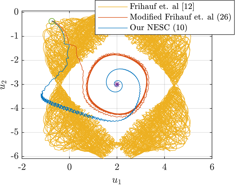
Figure 1: Input trajectories from an initial condition $\boldsymbol{u}(0)$ (denoted by $\circ$) towards $\boldsymbol{u}^{*}$ (denoted by $*$).

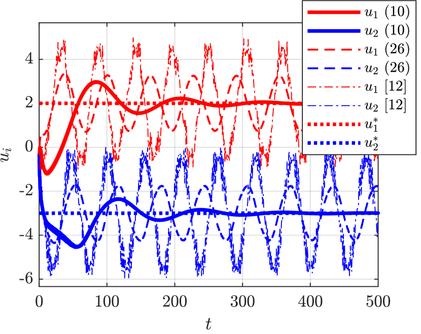
Figure 2: Time evolution of inputs $u_{1}$ and $u_{2}$ for the proposed NESC algorithm (solid line), the original algorithm in [10] (dash dot line) and the filtered version of the algorithm in [10] (dashed lines).

IV-B Fixed demand problem

In the second simulation example, we consider the problem of determining the production outputs $u_{i}\in\mathbb{R}$ so that $N$ producers minimize their cost and meet the some fixed demand $U_{d}\in\mathbb{R}$ (see the power generator examples in [36] [37]). The producers do not know the exact analytic form of their cost functions, which are given by:

$$J_{i}(u_{i},\lambda)=u_{i}(u_{i}-2U_{i})-\lambda u_{i},$$ (27)

where the first part corresponds to the unknown part of their cost and $\lambda u_{i}$ corresponds to the profit made by selling the commodity at the price $\lambda$. The last agent in this game is the market regulator whose goal is to balance supply and demand via the commodity price, by adopting the following cost function:

$$J_{N+1}(\boldsymbol{u},\lambda)=\lambda(-U_{d}+\Sigma_{i=1}^{N}u_{i}).$$ (28)

The producers and the market regulator use the algorithm in (10) to determine the production output and price, albeit the market regulator uses the real value of its gradient, measurable as the discrepancy between the supply and demand. In the simulations, we use the following parameters: $N=3$, $(U_{1},U_{2},U_{3})=(172,47,66)kW$, $a_{1}=a_{2}=a_{3}=20$, $(\kappa_{1},\kappa_{2},\kappa_{3})=(0.1778,0.1238,0.1824)$, $\epsilon_{i}=\tfrac{1}{3}$, $\gamma_{i}=0.02$ for all $i$, $U_{d}=350$ and zero initial conditions. In Figure 3, we observe that the agents converge to the NE of the game. Additionally, we test the sensitivity of the commodity price with respect to additive measurement noise that obeys a Gaussian distribution with zero mean and standard deviation $\sigma$ for all producers. For different values of the standard deviation $\sigma$, we perform 200 numerical simulations. Next, we take the last 250 seconds of each simulation and sample it every 1 second. We group the resulting prices $\lambda(t)$ into bins of width 0.05, and plot the frequency of each bin. Three such plots are shown on Figure 4. We observe that the price frequency plots seem to follow a Gaussian-like distribution.

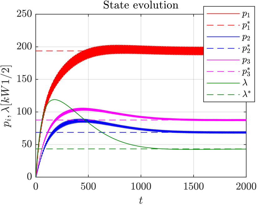
Figure 3: Time evolution of states in the fixed demand problem.

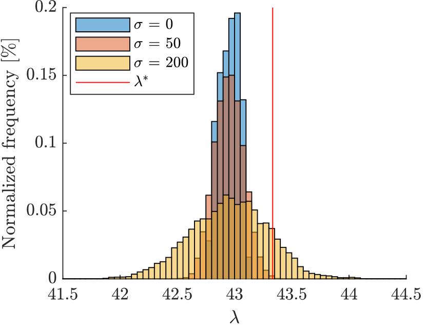
Figure 4: Price frequency distribution for three different cases.

V Conclusion

Monotone Nash equilibrium problems without constraints can be solved via zeroth-order methods that leverage the properties of the continuous-time Golden ratio algorithm and ESC theory based on hybrid dynamical systems.

-A On the projection case

In this appendix, we show why the usual Lyapunov function candidate as in (19), [4], [26], [27], [28], cannot be used for the projected version of the proposed algorithm. In the simplest projected version, we would have projections onto convex sets as in [25]:

$$\begin{bmatrix}\dot{\boldsymbol{z}}\\ \dot{\boldsymbol{u}}\end{bmatrix}=\begin{bmatrix}\left(-\boldsymbol{z}+\boldsymbol{u}\right)\\ \left(-\boldsymbol{u}+\mathrm{proj}_{\Omega}(\boldsymbol{z}-F(\boldsymbol{u})\right))\end{bmatrix}.$$ (29)

Let us show a case where the Lyapunov function candidate in (19) increases. In Figure 5, we consider $F(\boldsymbol{u})=\operatorname{col}\left({u_{2},-u_{1}}\right)$, that the convex set $\boldsymbol{\Omega}$ is given by the blue set and that the initial point is characterized by $\boldsymbol{u}=\boldsymbol{z}=[0,u_{2}]^{\top}$. The dotted lines represent the level sets of the Lyapunov function. The blue arrow represents the vector $-F(\boldsymbol{u})$, while the red one represents $-\boldsymbol{u}+\mathrm{proj}_{\Omega}(\boldsymbol{z}-F(\boldsymbol{u})$. We can see that the Lyapunov function does increase. For a different modulus of the pseudogradient vector, it is always possible to construct a convex set for which the Lyapunov function candidate increases. We conclude that a different Lyapunov candidate must be used to prove convergence in presence of constraints, which currently represents an open research problem.

Figure 5: Blue arrow denotes the negative vector of $F(\boldsymbol{u})=\operatorname{col}\left({u_{2},u_{1}}\right)$, while the purple area represents the set $\Omega$; level sets of the Lyapunov function are represented with doted lines; $\boldsymbol{u}^{*}$ is the NE; $\boldsymbol{p}=\mathrm{proj}_{\Omega}(\boldsymbol{u}-F(\boldsymbol{u}))$. For the case when $\boldsymbol{u}=\boldsymbol{z}$, derivative $\dot{\boldsymbol{u}}=-\boldsymbol{u}+\boldsymbol{p}$ is denoted with the red arrow. As the vector points outside of the level set, the Lyapunov function increases.

References

• [1] A.-H. Mohsenian-Rad, V. W. Wong, J. Jatskevich, R. Schober, and A. Leon-Garcia, “Autonomous demand-side management based on game-theoretic energy consumption scheduling for the future smart grid,” IEEE transactions on Smart Grid, vol. 1, no. 3, pp. 320–331, 2010.
• [2] W. Saad, Z. Han, H. V. Poor, and T. Basar, “Game-theoretic methods for the smart grid: Game-theoretic methods for the smart grid: An overview of microgrid systems, demand-side management, and smart grid communications,” IEEE Signal Processing Magazine, vol. 29, pp. 86–105, 2012.
• [3] Z. Ma, D. S. Callaway, and I. A. Hiskens, “Decentralized charging control of large populations of plug-in electric vehicles,” IEEE Transactions on control systems technology, vol. 21, no. 1, pp. 67–78, 2011.
• [4] S. Grammatico, “Dynamic control of agents playing aggregative games with coupling constraints,” IEEE Transactions on Automatic Control, vol. 62, no. 9, pp. 4537–4548, 2017.
• [5] S. Li, W. Zhang, J. Lian, and K. Kalsi, “Market-based coordination of thermostatically controlled loads—part i: A mechanism design formulation,” IEEE Transactions on Power Systems, vol. 31, no. 2, pp. 1170–1178, 2015.
• [6] W. Lin, Z. Qu, and M. A. Simaan, “Distributed game strategy design with application to multi-agent formation control,” in 53rd IEEE Conference on Decision and Control, pp. 433–438.
• [7] P. Yi and L. Pavel, “An operator splitting approach for distributed generalized Nash equilibria computation,” Automatica, vol. 102, pp. 111–121, 2019.
• [8] D. Gadjov and L. Pavel, “Distributed GNE seeking over networks in aggregative games with coupled constraints via forward-backward operator splitting,” in 2019 IEEE 58th Conference on Decision and Control (CDC), pp. 5020–5025.
• [9] J. R. Marden, G. Arslan, and J. S. Shamma, “Cooperative control and potential games,” IEEE Transactions on Systems, Man, and Cybernetics, Part B (Cybernetics), vol. 39, no. 6, pp. 1393–1407, 2009.
• [10] P. Frihauf, M. Krstic, and T. Basar, “Nash equilibrium seeking in noncooperative games,” IEEE Transactions on Automatic Control, vol. 57, no. 5, pp. 1192–1207, 2011.
• [11] T. Goto, T. Hatanaka, and M. Fujita, “Payoff-based inhomogeneous partially irrational play for potential game theoretic cooperative control: Convergence analysis,” in 2012 IEEE American Control Conference (ACC), pp. 2380–2387.
• [12] J. R. Marden and J. S. Shamma, “Revisiting log-linear learning: Asynchrony, completeness and payoff-based implementation,” Games and Economic Behavior, vol. 75, no. 2, pp. 788–808, 2012.
• [13] M. Krstić and H.-H. Wang, “Stability of extremum seeking feedback for general nonlinear dynamic systems,” Automatica, vol. 36, no. 4, pp. 595–601, 2000.
• [14] Y. Tan, D. Nešić, and I. Mareels, “On non-local stability properties of extremum seeking control,” Automatica, vol. 42, no. 6, pp. 889–903, 2006.
• [15] A. Ghaffari, M. Krstić, and D. NešIć, “Multivariable newton-based extremum seeking,” Automatica, vol. 48, no. 8, pp. 1759–1767, 2012.
• [16] H.-B. Dürr, M. S. Stanković, C. Ebenbauer, and K. H. Johansson, “Lie bracket approximation of extremum seeking systems,” Automatica, vol. 49, no. 6, pp. 1538–1552, 2013.
• [17] S. Krilašević and S. Grammatico, “Learning generalized nash equilibria in multi-agent dynamical systems via extremum seeking control,” Automatica, vol. 133, p. 109846, 2021.
• [18] S.-J. Liu and M. Krstić, “Stochastic Nash equilibrium seeking for games with general nonlinear payoffs,” SIAM Journal on Control and Optimization, vol. 49, no. 4, pp. 1659–1679, 2011.
• [19] J. I. Poveda and A. R. Teel, “A framework for a class of hybrid extremum seeking controllers with dynamic inclusions,” Automatica, vol. 76, pp. 113–126, 2017.
• [20] J. I. Poveda and M. Krstić, “Fixed-time gradient-based extremum seeking,” in 2020 IEEE American Control Conference (ACC), pp. 2838–2843.
• [21] F. Facchinei and J.-S. Pang, Finite-dimensional variational inequalities and complementarity problems.   Springer Science & Business Media, 2007.
• [22] H. H. Bauschke, P. L. Combettes et al., Convex analysis and monotone operator theory in Hilbert spaces, 2nd ed.   Springer, 2011, vol. 408.
• [23] G. M. Korpelevich, “The extragradient method for finding saddle points and other problems,” Matecon, vol. 12, pp. 747–756, 1976.
• [24] Y. Censor, A. Gibali, and S. Reich, “The subgradient extragradient method for solving variational inequalities in hilbert space,” Journal of Optimization Theory and Applications, vol. 148, no. 2, pp. 318–335, 2011.
• [25] Y. Malitsky, “Golden ratio algorithms for variational inequalities,” Mathematical Programming, pp. 1–28, 2019.
• [26] R. I. Boţ and E. R. Csetnek, “A dynamical system associated with the fixed points set of a nonexpansive operator,” Journal of dynamics and differential equations, vol. 29, no. 1, pp. 155–168, 2017.
• [27] M. Bianchi and S. Grammatico, “Continuous-time fully distributed generalized nash equilibrium seeking for multi-integrator agents,” Automatica, vol. 129, p. 109660, 2021.
• [28] R. I. Bot, E. R. Csetnek, and P. T. Vuong, “The forward-backward-forward method from continuous and discrete perspective for pseudo-monotone variational inequalities in hilbert spaces,” European Journal of Operational Research, 2020.
• [29] D. Gadjov and L. Pavel, “On the exact convergence to Nash equilibrium in monotone regimes under partial-information,” in 2020 59th IEEE Conference on Decision and Control (CDC), 2020, pp. 2297–2302.
• [30] T. Başar and G. J. Olsder, Dynamic noncooperative game theory.   SIAM, 1998.
• [31] R. Goebel, R. G. Sanfelice, and A. R. Teel, “Hybrid dynamical systems,” IEEE control systems magazine, vol. 29, no. 2, pp. 28–93, 2009.
• [32] H. K. Khalil, Nonlinear systems.   Prentice Hall, 2002.
• [33] W. Wang, A. R. Teel, and D. Nešić, “Analysis for a class of singularly perturbed hybrid systems via averaging,” Automatica, vol. 48, no. 6, pp. 1057–1068, 2012.
• [34] J. I. Poveda and N. Li, “Robust hybrid zero-order optimization algorithms with acceleration via averaging in time,” Automatica, vol. 123, p. 109361, 2021.
• [35] S. Grammatico, “Comments on “Distributed robust adaptive equilibrium computation for generalized convex games”[Automatica 63 (2016) 82–91],” Automatica, vol. 97, pp. 186–188, 2018.
• [36] M. Aunedi, D. Skrlec, and G. Strbac, “Optimizing the operation of distributed generation in market environment using genetic algorithms,” in MELECON 2008 14th IEEE Mediterranean Electrotechnical Conference, pp. 780–785.
• [37] A. Pantoja and N. Quijano, “A population dynamics approach for the dispatch of distributed generators,” IEEE Transactions on Industrial Electronics, vol. 58, no. 10, pp. 4559–4567, 2011.