Traditional credibility analysis of risks in insurance is based on the random effects model, where the heterogeneity across the policyholders is assumed to be time-invariant. One popular extension is the dynamic random effects (or state-space) model. However, while the latter allows for time-varying heterogeneity, its application to the credibility analysis should be conducted with care due to the possibility of negative credibilities per period [see Pinquet (2020a)]. Another important but under-explored topic is the ordering of the credibility factors in a monotonous manner—recent claims ought to have larger weights than the old ones. This paper shows that the ordering of the covariance structure of the random effects in the dynamic random effects model does not necessarily imply that of the credibility factors. Subsequently, we show that the state-space model, with AR(1)-type autocorrelation function, guarantees the ordering of the credibility factors. Simulation experiments and a case study with a real dataset are conducted to show the relevance in insurance applications.

Keywords: Dependence, Posterior ratemaking, Credibility, Dynamic random effects

JEL Classification: C300

1 Introduction

Insurers use credibility theory to adjust a policyholder’s premium based on past claim history. Typically, the a priori risk premium is first determined by the policyholder’s observable risk characteristics. Then the a posteriori premium is expressed as weighted sums of the past claims, and these weights are called credibility factors. The baseline model that underlies many of the early contributions in credibility theory is the static random effects model. In this case, a posteriori premium is expressed as a weighted sum of two terms: the sample mean and a priori risk premium. Consequently, a posteriori premium imposes the same credibility factors to each claim regardless of its seniority. Motivated by this downside of the time-invariant credibility factors, the literature has considered the age of claims by imposing geometric decreasing credibility factors (Gerber and Jones, 1973; Gerber et al., 1975; Sundt, 1988).

An alternative way to account for the seniority of the claims is through the introduction of the dynamic random effects rather than static random effects [Bolancé et al. (2003)]. Subsequently, the seniority of the claims is indirectly considered by allowing the dependence between random effects to decrease as time lag increases. These models fall within the scope of state-space models (SSM) and are computationally intensive to deal with. In particular, they do not allow for closed-form conditional expectation in general, which may make them computationally inconvenient for a posteriori ratemaking [e.g., Brouhns et al. (2003) and Li et al. (2020)]. Furthermore, computing the conditional expectation requires the full specification of the dynamics of the unobserved random effect process, which may give rise to more mis-specification risk. Consequently, the forecasting in the dynamic random effect model is often approximated by the credibility premium. However, not all dynamic random effects models lead to sensible credibility premium in the insurance perspective. Recently, Pinquet (2020a) shows that the credibility coefficients associated with these models are not necessarily ensured to be non-negative. More precisely, Pinquet (2020a) shows that in Poisson dynamic random effects models where the random effect has an AR($p$)-type auto-covariance function, the non-negativity condition is not satisfied without parametric constraints on the auto-covariance function. This result has important implications as it demonstrates the limitations of the credibility approach when used semi-parametrically, that is when actuarial meaningfulness is not considered.

This study furthers this investigation of dynamic random effects models, in a similar spirit as Pinquet (2020a). We focus on another important but thus far overlooked property of whether the credibility factors are decreasing in seniority. While this property is a motivation of the dynamic random effects in actuarial perspective [e.g., Pinquet et al. (2001); Bolancé et al. (2003); Lu (2018)], until now, it has not been formally checked in the literature. We start our analysis with a simple question: does a decreasing auto-correlation function (ACF) of the dynamic random effect suffice for the resulting credibility coefficients to be also decreasing in seniority? We show that this is generically not the case. This leads us to restrict our attention to dynamic random effect processes with AR(1) autocorrelation such as those introduced by (Grunwald et al., 2000). Under such an auto-correlation restriction, we show that the corresponding credibility factor is an increasing function of time as well as being non-negative.

The paper is organized as follows. Section 2 provides a brief introduction to the dynamic random effects models and credibility theory. In particular, we demonstrate that the ordering of the covariance does not always guarantee that of the credibility factor. Section 3 provides the specific formulation of the dynamic random effects model, which is guaranteed to have the ordered credibility factors. In Section 4, we perform a numerical study under various parameter settings. In Section 5, an empirical analysis is conducted on a real-life dataset.

2 The general setting and motivating examples

This section provides a quick reminder of the general setting, the definition of the credibility coefficients, and two motivating examples for which the credibility coefficients are not monotonously ordered.

2.1 Notation and definition

Let us assume that for each individual $i$, we observe claim-related variables $Y_{i,t}$ for policy year $t=1,...,T_{i}$. We denote the history of claims up to time $T_{i}$ by

$$\mathcal{F}_{i,T_{i}}:=\left\{Y_{i,t}\,\big{|}\,t=1,\ldots,T_{i},\right\},$$

and assume that the sequence $(Y_{i,t}:t=1,2,\cdots)$ is independent across different individuals $i$. In posterior ratemaking, it is interesting to predict $Y_{i,T_{i}+1}$ for each policyholder $i$ and upcoming year $T_{i}+1$, which is given as

$${\mathrm{E}}\left[Y_{i,T_{i}+1}|\mathcal{F}_{i,T_{i}}\right].$$ (1)

For the expository purpose, from now onward, we remove subscript $i$.

We say that a sequence of stationary random variables $(Y_{t}:t=1,2,\cdots)$ has positive covariance ordering if the autocovariance function (ACF) is decreasing in lag:

$${\rm Cov}\left[Y_{t},Y_{t+p}\right]>{\rm Cov}\left[Y_{t},Y_{t+q}\right],\quad\hbox{for all}\quad p,q,t=1,2,\cdots$$ (2)

satisfying $p<q$.

For the distributional assumption of the observed claims, we consider the reproductive exponential dispersion family (EDF) by McCullagh and Nelder (1989). They show a real-valued random variable ${\displaystyle Y}$ as belonging to the reproductive exponential dispersion model with mean parameter $u$ and dispersion parameter $\psi$ denoted by ${\rm ED}\left(u,\psi\right)$ and has a density function at $Y=y$ of the following form

$$h(y;u,\psi)\exp\left(\frac{\theta y-A(\theta)}{\psi}\right).$$

Here, $h$ is a suitable normalizing term, and $A$ is twice a continuously differentiable function satisfying

$$\theta=\left(A^{\prime}\right)^{-1}(u).$$

If $Y\sim{\rm ED}\left(u,\psi\right)$, we have

$${\mathrm{E}}\left[Y\right]=u\quad\hbox{and}\quad{\mathrm{V}ar}\left(Y\right)=V(u)\psi$$

where $V$, called the unit variance function, is defined by

$$V(u)=A^{\prime\prime}\left(\left(A^{\prime}\right)^{-1}(u)\right).$$

This study utilizes the following examples of distributions in EDF:

• ${\rm Pois}(\lambda)$: the Poisson distribution with parameter $\lambda$;

• ${\rm Gamma}(\lambda,\psi)$: the gamma distribution with mean $\lambda$ and variance $\lambda^{2}\psi$.

We use ${\rm Beta}(a,b)$ to denote the beta distribution with parameters $a,b$.

Finally, we also define three $T\times T$ matrices. We denote by $\boldsymbol{I}_{T}$ the identity matrix, $\boldsymbol{E}_{T}$ the matrix of 1, and $\boldsymbol{\Sigma}_{T,\rho}$ the Toeplitz matrix whose entries are given by

$$\left[\boldsymbol{\Sigma}_{T,\rho}\right]_{i,j}=\rho^{|i-j|},\quad i,j=1,\cdots,T.$$

where $\rho\in(-1,1)$. We recall the following well-known result concerning its inverse matrix:

$$(1-\rho^{2})\left(\boldsymbol{\Sigma}_{T,\rho}\right)^{-1}=\begin{cases}1,&(i,j)=(1,1),\quad\hbox{or}\quad(i,j)=(T,T);\\ 1+\rho^{2},&(i,j)\neq(1,1),(i,j)\neq(T,T),\quad\hbox{and}\quad i=j;\\ -\rho,&j=i+1\quad\hbox{or}\quad j=i-1;\\ 0,&\hbox{otherwise}.\end{cases}$$ (3)

2.2 Brief reminder of the credibility theory

While the conditional expectation in (1) is the best forecast in terms of the mean squared error (MSE), it can be problematic to communicate with the policyholders if it does not allow the closed form solution (Goulet, 1998). Alternatively, the credibility premium provides the efficient yet intuitive affine functional form of the premium, which facilitates communication with the policyholders. Formally, for a sequence of random variables $\left(Y_{t};t=1,2,\cdots\right)$ satisfying ${\mathrm{E}}\left[Y_{t}\right]=\lambda_{t}$, the credibility premium for time $T+1$ is defined by

$${\rm Prem}\left(Y_{1},\cdots,Y_{T}\right):=\widehat{\alpha}_{0}\lambda_{T+1}+\widehat{\alpha}_{1}Y_{1}+\cdots+\widehat{\alpha}_{T}Y_{T}$$ (4)

where

$$\left(\widehat{\alpha}_{0},\cdots,\widehat{\alpha}_{T}\right):=\operatorname*{arg\,min}\limits_{(\alpha_{0},\cdots,\alpha_{T})\in\mathbb{R}^{T+1}}{\mathrm{E}}\left[\left(Y_{T+1}-\left(\alpha_{0}\lambda_{T+1}+\alpha_{1}Y_{1}+\cdots+\alpha_{T}Y_{T}\right)\right)^{2}\right].$$ (5)

Here, $\widehat{\alpha}_{t}$ for $t=1,\cdots,T$ is referred to as the credibility factor, which can be interpreted as the contribution of $t$-th year observation to the credibility premium. This credibility premium, which is the best linear unbiased estimator (BLUE) of ${\mathrm{E}}\left[Y_{T+1}|\mathcal{F}_{T}\right]$, can be computed through [see Bühlmann and Gisler (2006)]:

$$\left(\widehat{\alpha}_{1},\cdots,\widehat{\alpha}_{T}\right)^{\prime}=\boldsymbol{\Sigma}_{T}^{-1}\left(\begin{array}[]{c}{\rm Cov}\left[Y_{1},Y_{T+1}\right]\\ {\rm Cov}\left[Y_{2},Y_{T+1}\right]\\ \vdots\\ {\rm Cov}\left[Y_{T},Y_{T+1}\right]\end{array}\right)$$ (6)

and

$$\widehat{\alpha}_{0}=\frac{{\mathrm{E}}\left[Y_{T+1}\right]-\sum\limits_{t=1}^{T}\widehat{\alpha}_{t}{\mathrm{E}}\left[Y_{t}\right]}{\lambda_{T+1}}$$ (7)

where $\boldsymbol{\Sigma}_{T}$ is a $T\times T$ covariance matrix defined by

$$\left[\boldsymbol{\Sigma}_{T}\right]_{i,j}={\rm Cov}\left[Y_{i},Y_{j}\right]$$

We say that the credibility premium is regular if

$$\widehat{\alpha}_{t}>0,\quad\hbox{for}\quad t=1,\ldots.$$

We note that negative credibility factors are highly undesirable for regulatory reasons, as they might give the wrong incentives of making claims to get lower premiums or even give rise to negative premiums, which is the synonym of arbitrage opportunities [e.g., Pinquet (2020a), Li et al. (2020)]. For the condition of the regular credibility premium, we refer to the study of Pinquet (2020a, b).

The following example shows the property of credibility factors under the static random effects model.

Example 1 (Static random effects model).

For a distribution function $G$, consider a random effect $R\sim G$ so that $Y_{j}$’s are conditionally independent for given $R$. Subsequently, after integrating the random effect, we obtain the joint distribution of $(Y_{1},\cdots,Y_{T},Y_{T+1})$. However, random effects models may not be ideal for the posterior ratemaking in insurance products mainly due the symmetric dependence structure. Consequently, old claims are equally treated as new claims in the determination of future premiums, which is clearly counterintuitive. More precisely, as the covariance matrix in (6) has the equi-covariance structure, the following identity holds:

$$\widehat{\alpha}_{1}=\cdots=\widehat{\alpha}_{T}.$$ (8)

Clearly, the credibility premium having the credibility factors of the form in (8) is counterintuitive when applied to insurance ratemaking, in the sense that the weight of old claims, for example, $\widehat{\alpha}_{1}$, is the same as the weight of new claims, for example, $\widehat{\alpha}_{T}$.

More realistically, one may depart from the equi-covariance assumption and consider a series of random variables $(Y_{t}:t=1,2,\cdots)$ specified as follows, which has the positive covariance ordering as in (2).

Example 2 (Dynamic random effects model).

Let us consider a dynamic random effects (or state-space) model comprising an unobserved process $(R_{t}:t=0,1,\cdots)$ (called state variable) and an observed process $(Y_{t}:t=1,2,\cdots)$. We also assume that for $t$ varying, $Y_{t}$’s are independent conditionally on $(R_{t}:t=1,2,\cdots)$, and their distribution depends on $R_{t}$ only. Consequently, the joint density function of $\left(Y_{1:T},R_{0:T}\right)$ can be expressed as

$$f\left(y_{1:T},r_{0:T}\right)=f\left(r_{0}\right)\prod\limits_{t=1}^{T}f(y_{t}|r_{t})f\left(r_{t}|r_{t-1}\right).$$

In other words, such a model has the causal chain:

$$\cdots$$

(9)

Consequently, the specification of the random effects model $\left(Y_{1:T},R_{0:T}\right)$ boils down to the specification of

1. The dynamics of the sequence $(R_{t}:t=0,1,\ldots)$.

2. The conditional distribution of $Y_{t}$ for given $R_{t}$ for each $t$.

Assuming that the sequence $(r_{t}:t=1,2,\cdots)$ has the positive covariance ordering, it is natural to ask whether more recent observations have more influence than the old observations in the determination of the premium—whether we have

$$\widehat{\alpha}_{1}\leq\cdots\leq\widehat{\alpha}_{T}.$$ (10)

under the framework of credibility theory. It will be shown in the next subsection that the positive covariance ordering of $(Y_{t})$ or $(R_{t})$ is not sufficient to guarantee (10).

2.3 Some motivating state-space counter-examples

This subsection provides two motivating examples of the stationary dynamic random effects model $(Y_{t})$, which has a positive covariance ordered random effects $(R_{t})$, without the credibility coefficients being monotonically decreasing in seniority.

Example 3 (Semi-parametric model).

Let us first consider the first dynamic random effects model pioneered by Bolancé et al. (2003). This model is semi-parametric in the sense that the auto-covariance of the dynamic random effect process is not constrained. We set $\sigma^{2}=1$, and take the estimate of the auto-correlation function from their paper (see their Table 1):

$$\rho_{1}=.733,\ \rho_{2}=.524,\ \rho_{3}=.504,\ \rho_{4}=.483,\ \rho_{5}=.401.$$

Then we compute the credibility coefficients with time invariant $\lambda_{t}=1$, to obtain the credibility coefficients which are equal to

$$\begin{pmatrix}\alpha_{3,T}\\ \alpha_{2,T}\\ \alpha_{1,T}\end{pmatrix}=\begin{pmatrix}0.29\\ 0.10\\ 0.14\end{pmatrix}$$

if $T=3$, or:

$$\begin{pmatrix}\alpha_{4,T}\\ \alpha_{3,T}\\ \alpha_{2,T}\\ \alpha_{1,T}\end{pmatrix}=\begin{pmatrix}0.28\\ 0.09\\ 0.11\\ 0.11\end{pmatrix}$$

if $T=4$, or:

$$\begin{pmatrix}\alpha_{5,T}\\ \alpha_{4,T}\\ \alpha_{3,T}\\ \alpha_{2,T}\\ \alpha_{1,T}\end{pmatrix}=\begin{pmatrix}0.27\\ 0.09\\ 0.10\\ 0.09\\ 0.05\end{pmatrix}$$

if $T=5$. In particular, in none of the three cases, the credibility coefficients are correctly ordered.

Example 4 (A parametric model).

The previous example shows the importance of putting constraints on the autocorrelation function of the dynamic random effect process rather than leaving it unconstrained. Let us now inspect a parametric model with a simple autocorrelation function.

Consider a state-space model that comprises a state process $(\boldsymbol{R}_{t}:t=0,1,\ldots)$ and observable time series $(Y_{t}:t=1,2,\ldots)$ of the following form:

1. The conditional distribution of $Y_{t}$ for given $\boldsymbol{R}_{t}:=\left(R_{t,1},R_{t,2}\right)$ is

   $$Y_{t}|\boldsymbol{R}_{t}\sim{\rm ED}\left(\lambda_{t}\left({R_{t,1}+R_{t,2}}\right),\psi\right).$$

2. $(R_{t,1}:t=0,1,\ldots)$ and $(R_{t,2}:t=0,1,\ldots)$ are independent processes such that $(R_{t,1}:t=0,1,\ldots)$ has AR(1)-type autocorrelation:

   $${\mathrm{E}}\left[R_{t,1}\right]=1,\quad{\mathrm{V}ar}\left(R_{t,1}\right)=\sigma_{1}^{2},\quad\hbox{and}\quad{\rm Cov}\left[R_{t_{1},1},R_{t_{2},1}\right]=\sigma_{1}^{2}\rho^{|t_{2}-t_{1}|},\quad t,t_{1},t_{2}\in\mathbb{N}_{0},$$ (11)

   and $R_{t,2}$ is time-invariant:

   $${\mathrm{E}}\left[R_{t,2}\right]=1,\quad{\mathrm{V}ar}\left(R_{t,2}\right)=\sigma_{2}^{2},\quad\hbox{and}\quad{\rm Cov}\left[R_{t_{1},2},R_{t_{2},2}\right]=\sigma_{2}^{2},\quad t,t_{1},t_{2}\in\mathbb{N}_{0}.$$ (12)

Models involving both time-invariant and time-varying random effects have previously been considered by Pinquet (2020a). Note that here, the process $(R_{t,1}+R_{t,2})$ is stationary but is generically non-Markov.

We can easily check that

$${\mathrm{V}ar}\left(Y_{t}\right)=\psi{\mathrm{E}}\left[V\left(R_{t,1}+R_{t,2}\right)\right]+\left({\mathrm{V}ar}\left(R_{t,1}\right)+{\mathrm{V}ar}\left(R_{t,2}\right)\right),$$

and

$${\rm Cov}\left[Y_{t_{1}},Y_{t_{2}}\right]=\sigma_{1}^{2}\rho^{|t_{1}-t_{2}|}+\sigma_{2}^{2}.$$

When $\psi=0$, the covariance matrix of $(Y_{1},\cdots,Y_{T})$ has the same structure as in (39). Consequently, $\psi\rightarrow 0$, Lemma 2 in B shows the following inequality

$$\widehat{\alpha}_{1}>\widehat{\alpha}_{j},\quad j=2,\cdots,t-1$$ (13)

which clearly shows that the credibility factors do not satisfy the increasing property in (10).

For a numerical illustration, we assume identity variance function $V$ and set parameters

$$\sigma_{1}^{2}=1,\quad\rho=0.8,$$

and

$$\lambda_{t}=1,\quad t=0,1,\cdots.$$

Table 1 shows the credibility factors for $T=5$ for various combinations of $\psi$ and $\sigma_{2}^{2}$. As expected, we have

$$\widehat{\alpha}_{1}>\widehat{\alpha}_{t},\quad t=2,\cdots,4$$

under Scenarios I and II with small $\psi=0.01$ and $0.1$, respectively.

Table 1: credibility factors for various combinations of $\psi$ and $\sigma_{2}^{2}$

Scenarios	Parameters	$\widehat{\alpha}_{1}$	$\widehat{\alpha}_{2}$	$\widehat{\alpha}_{3}$	$\widehat{\alpha}_{4}$	$\widehat{\alpha}_{5}$	monotonicity of $(\widehat{\alpha}_{j})_{j}$
I	$\psi=0.01$ and $\sigma_{2}^{2}=1$	0.046	0.011	0.011	0.042	0.805	no
II	$\psi=0.1$ and $\sigma_{2}^{2}=1$	0.049	0.030	0.050	0.158	0.600	no
III	$\psi=1$ and $\sigma_{2}^{2}=1$	0.086	0.093	0.118	0.169	0.260	yes
IV	$\psi=0.1$ and $\sigma_{2}^{2}=0.01$	0.003	0.009	0.034	0.137	0.554	yes

However, under Scenarios III and IV, which correspond to the relatively large value of $\psi=1$, we have the ordering of the credibility factors in (10).

Remark 1.

It is well known that the credibility model is equivalent to regressing $X_{t}$ on its lagged values. Therefore, the fact that the credibility coefficients, or equivalently the regression coefficients, are not necessarily ordered corresponds to also a well-known issue in the time series literature. Let us, for instance, consider ARMA(1,1) process $(Y_{t})$ defined by

$$Y_{t}=\phi Y_{t-1}+e_{t}+\theta-\theta e_{t-1},$$

where $(e_{t})$ represents an unobserved white noise series with zero mean and variance $\sigma_{e}^{2}$. Following the standard procedure, we have

$${\mathrm{V}ar}\left(Y_{t}\right)=\frac{1-2\phi\theta+\theta^{2}}{1-\phi^{2}}\sigma_{e}^{2}\quad\hbox{and}\quad{\rm Cov}\left[Y_{t},Y_{t+1}\right]=\phi{\mathrm{V}ar}\left(Y_{t}\right)-\theta\sigma_{e}^{2}$$

and

$${\rm Cov}\left[Y_{t},Y_{t+k}\right]=\phi{\rm Cov}\left[Y_{t},Y_{t+k-1}\right],\quad\hbox{for}\quad k\geq 2.$$

Now, consider ARMA(1,1) process $(Y_{t})$ with

$$(\phi,\theta,\sigma_{e}^{2})=(0.5,-0.2,1.0).$$

Clearly, $(Y_{t})$ has positive covariance ordering. However, the ordering of the credibility factors in (10) is not satisfied. For example, when $T=5$, the credibility factors in (5) are given by

$$(\widehat{\alpha}_{1},\cdots,\widehat{\alpha}_{5})=(0.001,-0.006,0.028,-0.140,0.700),$$

which shows neither monotonically increasing nor monotonically decreasing pattern.

This issue has (partly) prompted the introduction of alternative time series models that ensure the correct ordering, such as the Harvey-Fernandez model (see Section 3).

3 Ordering of credibility factors under the AR(1) state-space model

The examples in Section 2.3 show that the monotonicity of the ACF of the state process $(R_{t})$ does not guarantee the ordering of the credibility factors corresponding to observable time series $(Y_{t})$. In some sense, these counter-examples are not surprising, as Pinquet (2020a) has already found examples for which positive ACF does not necessarily lead to positive credibility coefficients. In other words, for the credibility coefficients to be “well behaved,” generally, further restrictions on the ACF are required. This section discusses the ordering of credibility factors under the dynamic random effects model and shows that the dynamic random effects model with the random effects having an AR(1)-type ACF ensures the ordering of the credibility coefficients.

3.1 Model specification and main result

Model 1 (AR(1) State-Space Model).

Consider a state-space model comprising a state process $(R_{t}:t=0,1,\ldots)$ and observable time series $(Y_{t}:t=1,2,\ldots)$ of the following form:

1. Conditional distribution of $Y_{t}$ for given $R_{t}$ is

   $$Y_{t}|R_{t}\sim{\rm ED}\left(\lambda_{t}R_{t},\psi\right)$$ (14)

   where ${\rm ED}\left(\lambda_{t}R_{t},\psi\right)$ denotes EDF with mean $\lambda_{t}R_{t}$, dispersion parameter $\psi$, and variance function $V(\cdot)$.

2. A state process $(R_{t}:t=0,1,\ldots)$ has stationary Markov property, and we further assume ${\mathrm{E}}\left[R_{t}\right]=1$ for $t=0,1,\cdots$. Owing to stationary property, ${\mathrm{V}ar}\left(R_{t}\right)$’s are time-invariant constant, and we denote it as

   $${\mathrm{V}ar}\left(R_{t}\right)=\sigma^{2},\quad t=0,1,\cdots$$ (15)

   for convenience.

3. We further assume that the ACF satisfies

   $${\rm Cov}\left[R_{t_{1}},R_{t_{2}}\right]=\sigma^{2}\rho^{|t_{2}-t_{1}|},\quad t_{1}\neq t_{2}$$ (16)

   for $t_{1},t_{2}=0,1,\cdots$.

It is straightforward to observe that the closed-form expression of the marginal mean and variance of $Y_{t}$ is given by

$${\mathrm{E}}\left[Y_{t}\right]=\lambda_{t}\quad\hbox{and}\quad{\mathrm{V}ar}\left(Y_{t}\right)=\psi{\mathrm{E}}\left[V(\lambda_{t}R_{t})\right]+\lambda_{t}^{2}\sigma^{2},$$ (17)

and the marginal covariance of $Y_{t_{1}}$ and $Y_{t_{2}}$ is given by

$${\rm Cov}\left[Y_{t_{1}},Y_{t_{2}}\right]=\lambda_{t_{1}}\lambda_{t_{2}}\sigma^{2}\rho^{|t_{1}-t_{2}|},\quad t_{1}\neq t_{2}.$$ (18)

We first observe that the positive covariance ordering of $(Y_{t})$ is not guaranteed depending on the choice of $\lambda_{t}$’s. To ensure the positive covariance ordering of $(Y_{t})$, we restrict our attention to the standardized observations. Specifically, under the settings in Model 1, the standardized observations is defined as

$$Y_{t}^{*}=\frac{Y_{t}}{\lambda_{t}},\quad t=1,2,\cdots.$$

In particular, in insurance, standardized observations play a key role in ratemaking systems, and premiums are often expressed in terms of the standardized observations (Bühlmann and Gisler, 2006). For example, the credibility premium of $Y_{T+1}$ defined in (4) can be equivalently represented as

$${\rm Prem}\left(Y_{1},\cdots,Y_{T}\right):=\widehat{\alpha}_{0}+\widehat{\alpha}_{1}^{*}Y^{*}_{1}+\cdots+\widehat{\alpha}_{T}^{*}Y^{*}_{T},$$ (19)

where

$$\widehat{\alpha}_{1}^{*}=\lambda_{1}\widehat{\alpha}_{1},\ldots,\widehat{\alpha}_{T}^{*}=\lambda_{T}\widehat{\alpha}_{T}$$ (20)

with $\widehat{\alpha}_{t}$’s given by (5). We say the credibility premium is positively isotonic if

$$\widehat{\alpha}_{1}^{*}\leq\cdots\leq\widehat{\alpha}_{T}^{*}.$$ (21)

We emphasize the terminology “positive” here. While we say the sequence has the positive covariance ordering if the ACF is decreasing function in time as in (2), we define the credibility premium to be positively ordered if the credibility factors are increasing function in time as in (21).

We now have all the necessary ingredients to introduce the main result of the study. The following theorem says that the monotonicity of the credibility coefficients is necessarily satisfied when the dynamic random effect has an AR(1)-type ACF.

Theorem 1.

Consider the time series $(Y_{t})$ in the state-space model in Model 1 and assume that $\left(\lambda_{1:t}\right)$ is time-invariant:

$$\lambda_{1}=\cdots=\lambda_{T}.$$ (22)

Subsequently, the time series $(Y_{t}^{*})$ has positive covariance ordering, and credibility factors corresponding to the standardized observations are positively isotonic. Specifically, $\widehat{\alpha}_{1}^{*},\ldots,\widehat{\alpha}_{T}^{*}$ in (19) satisfy the following inequality

$$\widehat{\alpha}_{1}^{*}\leq\cdots\leq\widehat{\alpha}_{T}^{*},$$

where the equality holds if and only if $\rho=0$.

Proof.

The proof for the positive covariance ordering of $(Y_{t}^{*})$ is immediate from the following

$${\rm Cov}\left[Y_{t_{1}}^{*},Y_{t_{2}}^{*}\right]=\sigma^{2}\rho^{|t_{1}-t_{2}|},\quad t_{1}\neq t_{2}$$

obtained from (18). For the proof of the remaining part, see Appendix A. ∎

We note that the investigation of the ordering of the credibility factors can be less meaningful if (22) is not satisfied. If we do not assume (22), neither $(Y_{t})$ nor $(Y_{t}^{*})$ is guaranteed to be stationary so that discussion of the corresponding credibility factors can be void. Indeed, it will be shown in Section 4.1 through a numerical study that the credibility factors change drastically according to the choice of $(\lambda_{1},\cdots,\lambda_{T})$. Consequently, we conclude that the concept of positively isotonic is more sensible with the condition in (22). In C, for the completeness of the paper, we also provide results on the ordering of the credibility factors without assuming the condition in (22).

3.2 Parametric examples

The class of time series satisfying the correlation structure in (16), which is characterized by

$${\mathrm{E}}\left[R_{t}|R_{t-1}\right]=\phi_{1}R_{t-1}+\phi_{2},$$

for real numbers $\phi_{1}$ and $\phi_{2}$, includes a wide range of AR(1) models (e.g., Grunwald et al. (2000)). Let us now provide some examples.

Example 5 (Beta-Gamma autoregressive process of the first-order (BGAR(1))).

We say that $(R_{t}:t=0,1,\cdots)$ is a BGAR(1) [see Lewis et al. (1989)] with parameter $(\gamma_{1},\gamma_{2},\rho)\in\mathbb{R}_{+}^{3}$ if it satisfies

$$R_{t}=B_{t}R_{t-1}+G_{t},\quad t=0,1,\cdots,$$

where $(B_{t}:t=0,1,\cdots)$ and $(G_{t}:t=0,1,\cdots)$ are mutually independent sequences of i.i.d. random variables satisfying

$$B_{t}\sim{\rm Beta}\left(\gamma_{1}\rho,\gamma_{1}(1-\rho)\right)\quad\hbox{and}\quad G_{t}\sim{\rm Gamma}\left(\frac{\gamma_{1}(1-\rho)}{\gamma_{2}},\frac{1}{\gamma_{1}(1-\rho)}\right),\quad t=0,1,\cdots.$$

Subsequently, we remark that if $R_{t-1}\sim{\rm Gamma}(\gamma_{1}/\gamma_{2},1/\gamma_{1})$, then by the property of the beta distribution, we have

$$B_{t}R_{t-1}\sim{\rm Gamma}\left(\frac{\gamma_{1}\rho}{\gamma_{2}},\frac{1}{\gamma_{1}\rho}\right)$$

, and hence, the marginal distribution of $R_{t}$ is given by

$$R_{t}\sim{\rm Gamma}\left(\frac{\gamma_{1}}{\gamma_{2}},\frac{1}{\gamma_{1}}\right).$$

Finally, the serial variance and covariance of $(R_{t})$ are obtained as

$${\mathrm{V}ar}\left(R_{t}\right)=\frac{\gamma_{1}}{\gamma_{2}^{2}}\quad\hbox{and}\quad{\rm Cov}\left[R_{t},R_{t-\ell}\right]=\rho^{t-\ell}\frac{\gamma_{1}}{\gamma_{2}^{2}},\quad\ell=0,1,\cdots.$$

The following two examples of state-space model are described by a BGAR(1) with parameter $(\gamma_{1},\gamma_{2},\rho)$. For the identification purpose, we assume that $\gamma_{1}=\gamma_{2}=1/\sigma^{2}$ so that ${\mathrm{E}}\left[R_{t}\right]=1$ and ${\mathrm{V}ar}\left(R_{t}\right)=\sigma^{2}$. Note that we also have ${\mathrm{E}}\left[R^{3}\right]=(2\sigma^{2}+1)(\sigma^{2}+1)$.

Example 6 (A dynamic gamma-gamma model).

Consider the state-space model in Model 1 with observable time series $(Y_{t}:t=1,2,\cdots)$ and state variable $(R_{t}:t=1,2,\cdots)$ with the following specification:

• $(R_{t}:t=1,2,\cdots)$ is given by a BGAR(1) with parameter $(\gamma,\gamma,\rho)$ with $\gamma=1/\sigma^{2}$.

• The observation $Y_{t}$ conditional on $R_{t}$ is given by

  $$Y_{t}|R_{t}\sim{\rm Gamma}\left(\lambda_{t}R_{t},\psi\right).$$ (23)

Subsequently, for $t,t_{1},t_{2}\in\mathbb{N}$ and $t_{1}\neq t_{2}$, we have

$${\mathrm{E}}\left[Y_{t}\right]=\lambda_{t},\quad{\mathrm{V}ar}\left(Y_{t}\right)=\lambda_{t}^{2}\left(\psi\left(1+\sigma^{2}\right)+\sigma^{2}\right),\quad\hbox{and}\quad{\rm Cov}\left[Y_{t_{1}},Y_{t_{2}}\right]=\lambda_{t_{1}}\lambda_{t_{2}}\rho^{|t_{1}-t_{2}|}\sigma^{2}.$$

Furthermore, using Theorem 2 in A, $\widehat{\alpha}_{1}^{*},\ldots,\widehat{\alpha}_{T}^{*}$ in (19) is obtained as

$$\left(\widehat{\alpha}_{1}^{*},\ldots,\widehat{\alpha}_{T}^{*}\right)=\rho\left(1-\rho^{2}\right)\sigma^{2}\lambda_{T+1}v_{T}\left(u_{1},\ldots,u_{T}\right)\frac{1}{\left(1+\sigma^{2}\right)\psi},$$ (24)

where $u_{1},\ldots,u_{T}$ and $v_{T}$ are defined in Definition 1 in A. Clearly, the credibility premium is regular. Furthermore, if $\lambda_{1}=\cdots=\lambda_{T}$, the time series $(Y_{t})$ has positive covariance ordering. Finally, with the help of Lemma 1, the results in (24) clearly show that the credibility premium is regular. This confirms the result in Theorem 1.

Example 7 (A dynamic Poisson-gamma model).

Consider the same state-space model in Model 1, where the distributional assumption in (23) is replaced by

$$Y_{t}|R_{t}\sim{\rm Pois}\left(\lambda_{t}R_{t}\right).$$ (25)

Subsequently, for $t,t_{1},t_{2}\in\mathbb{N}$ and $t_{1}\neq t_{2}$, we have

$${\mathrm{E}}\left[Y_{t}\right]=\lambda_{t},\quad{\mathrm{V}ar}\left(Y_{t}\right)=\lambda_{t}+\lambda_{t}^{2}\sigma^{2},\quad\hbox{and}\quad{\rm Cov}\left[Y_{t_{1}},Y_{t_{2}}\right]=\lambda_{t_{1}}\lambda_{t_{2}}\sigma^{2}\rho^{|t_{1}-t_{2}|}.$$

Similar to Example 6, Theorem 2 in Appendix A shows that $\widehat{\alpha}_{1}^{*},\ldots,\widehat{\alpha}_{T}^{*}$ in (19) are obtained as

$$\left(\widehat{\alpha}_{1}^{*},\ldots,\widehat{\alpha}_{T}^{*}\right)=\rho\left(1-\rho^{2}\right)\sigma^{2}\lambda_{T+1}v_{T}\left(u_{1}\lambda_{1},\ldots,u_{T}\lambda_{T}\right).$$

where $u_{1},\ldots,u_{T}$, and $v_{T}$ are defined in Definition 1 in Appendix A. Clearly, the credibility premium is regular. Furthermore, if $\lambda_{1}=\cdots=\lambda_{T}$, the time series $(Y_{t})$ has positive covariance ordering, and credibility premium is positively isotonic by Lemma 1. This confirms the result in Theorem 1.

Remark 2.

Under certain circumstances, the credibility premium is guaranteed to be positively isotonic without assuming time-invariant $(\lambda_{t})$ as in (22). Let us, for instance, reconsider Example 6. As the unit variance function of Gamma distribution is $V(x)=x^{2}$, part ii of Corollary 1 in C shows that the credibility premium is guaranteed to be positively isotonic without the assumption in (22).

Similar ideas can be used to come up with the example whose (non-standard) credibility factors are positively ordered without assuming (22). Consider the time series $(Y_{t})$ in (7). As the unit variance function of Poisson distribution is the identity function—$V(x)=x$—part i of Corollary 1 in C shows that the credibility factors satisfy

$$\widehat{\alpha}_{1}\leq\cdots\leq\widehat{\alpha}_{T}$$

regardless of the assumption in (22).

However, as we have already discussed, neither the time series $(y_{t})$ nor $(y_{t}^{*})$ is stationary. Consequently, it is less meaningful to discuss the ordering of credibility factors without assuming time-invariant $(\lambda_{t})$ as in (22).

Finally, note that besides BGAR(1) used in Examples 6 and 7, there are other stationary processes with stationary, gamma distribution, as well as AR(1)-type auto-covariance function. In the following, let us give two well-known examples.

Example 8 (Autoregressive gamma process (ARG)).

The ARG process is the exact time-discretization of the square-root diffusion process and has been introduced into the ratemaking literature by Lu (2018). This process is Markov and is mostly conveniently specified through the conditional Laplace transform:

$$\mathbb{E}[\exp(-sR_{t+1})\mid R_{t}]=\frac{1}{(1+cs)^{\delta}}\exp\Big{(}-\frac{\rho s}{1+cs}R_{t}\Big{)},\qquad\forall s\geq 0,$$ (26)

where $\rho\in[0,1]$, and $c,\delta>0$. By taking first derivative with respect to $s$, it is easily shown that $\mathbb{E}[R_{t+1}|R_{t}]=\rho R_{t}+c\delta$.

As this model has the same auto-covariance function as the above BGAR(1) process, it gives rise to the same credibility coefficients in a state-space context.

Example 9 (Gamma autoregressive process).

Gaver and Lewis (1980) consider the process $(R_{t})$ defined by

$$R_{t+1}=\rho R_{t}+\epsilon_{t+1},$$

where the innovation process $(\epsilon_{t})$ is i.i.d. They work out the distribution of the latter such that process $(R_{t})$ is marginally gamma distributed. For this example, by definition, we have $\mathbb{E}[R_{t+1}|R_{t}]=\rho R_{t}+\mathbb{E}[\epsilon_{t}]$.

3.3 Comparison with Harvey and Fernandez’s approach

The dynamic, AR(1)-type random effects model considered above is a state-space model with an exogenous state process. In other words, the conditional distribution of $R_{t}$ given the past of both processes $(R_{t})$ and $(y_{t})$ only depends on its own past but not on that of $(y_{t})$. Alternatively, the time series literature has also proposed state-space models with non-exogenous or endogenous state process, which does not have the causal chain (9). One such example is the count time series model of Harvey and Fernandes (1989), which has been applied in the actuarial literature by Bolancé et al. (2007); Abdallah et al. (2016). This model, which is based on the Poisson-gamma conjugacy, is such that at any time $t$, both the filtering density $R_{t}|(Y_{1},\cdots,Y_{t})$ and the predictive density $R_{t+1}|(Y_{1},\cdots,Y_{t})$ are gamma. More precisely, the joint dynamics of $(R_{t},y_{t}:t=0,1,\ldots)$ is defined as follows:

• (Initial value) $R_{1}\sim{\rm Gamma}^{*}(a_{0},b_{0})$ with $a_{0}=b_{0}$.

• (measurement equation) For each $t$,

  $$Y_{t}|(R_{t},R_{t-1},...,Y_{t-1},...)\sim{\rm Pois}\left(\lambda_{t}R_{t}\right),$$

• (Updating formula) If

  $$R_{t}|(Y_{1},\cdots,Y_{t})=(y_{1},\cdots,y_{t})\sim{\rm Gamma}^{*}(a_{t},b_{t}),$$

  then the one-step-ahead conditional distribution of the random effect is given by

  $$R_{t+1}|(Y_{1},\cdots,Y_{t})=(y_{1},\cdots,y_{t})\sim{\rm Gamma}^{*}(\alpha a_{t},\alpha b_{t})$$ (27)

  for a time-invariant constant $\alpha\in(0,1]$. Moreover, these authors show that $a_{t}$ and $b_{t}$ are some affine functions of $(y_{1},\cdots,y_{t})$.

Here, ${\rm Gamma}^{*}(a_{0},b_{0})$ denotes the gamma distribution with shape parameter $a_{0}$ and rate parameter $b_{0}$.

A direct consequence of this specification, and especially equation (27), is the following exponential moving average predictive mean:

$${\mathrm{E}}\left[Y_{t+1}|Y_{1},\cdots,Y_{t}\right]=\lambda_{t+1}\frac{a_{0}+\sum\limits_{\tau=1}^{t}\alpha^{-\tau}Y_{t}}{a_{0}+\sum\limits_{\tau=1}^{t}\alpha^{-\tau}\lambda_{t}}.$$ (28)

As the conditional expectation is linear, the credibility forecast and the conditional expectation coincide. Therefore, this is yet another model in which the credibility coefficients form a decreasing (indeed geometric) sequence.

The major differences between Model 1 and the model of Harvey and Fernandez are three-fold. First, unlike Model 1, Harvey and Fernandes (1989)’s model is specific to the models with conditional Poisson distribution. Second and more importantly, the dynamics of the random effects process $(R_{t}:t=0,1,\ldots)$ defined in Harvey and Fernandes (1989) is nonstationary, in the sense that the marginal distribution of $R_{t}$ is not time-invariant., even when $\lambda_{t}$ is time-variant. This non-stationarity makes the interpretation of this model considerably unnatural. Finally, recently, Boucher and Pigeon (2018) showed that, unlike random effects type models, the Harvey-Fernandez model has an undesirable numerical feature that the impact of a single claim for an insured is excessively large for policyholders with a long driving experience. This makes it unappealing when it comes to retaining loyal and good drivers.

4 Numerical study

This section performs numerical studies on the credibility factors with the proposed methodology. First, in Section 4.1, we provide a numerical example showing that the state-space model in Model 1 is not necessarily positively isotonic. Subsequently, in Section 4.2, we analyze credibility premiums with the proposed model under various parameter settings in Model 1 and compare their performances to those of the exact premium in (1).

4.1 Numerical examples of credibility premiums which are not positively isotonic

In Section 2.3, we show that the credibility premium under a state-space model is not necessarily positively isotonic, although it has the decreasing covariance property. In this subsection, we show, by example, that even a state-space model as in Model 1 can have credibility premiums that are not positively isotonic. While Theorem 1 shows that credibility factors under the assumptions in Model 1 are positively isotonic if time-invariant fixed effects are assumed, we may have credibility factors that are not positively isotonic with time-varying fixed effects.

First, consider the credibility premium under the settings in Example 7 with $t=5$, $\sigma^{2}=0.5$, and $\psi=0.5$. For other parameters, consider the combination of $\rho=0.3,0.6$ and

$$\left(\lambda_{1},\cdots,\lambda_{5}\right)=\begin{cases}(1,1,1,1,1);\\ (0.001,0.01,0.1,1,10);\\ (10,1,0.1,0.01,0.001);\\ \end{cases}$$

with $\lambda_{6}=1$. Table 2 shows the credibility factors calculated in (24).

Columns corresponding to Case 1.a and Case 2.a in Table 2 represent time-invariant fixed effects. Clearly, credibility premiums in these cases are positively isotonic, which confirms Theorem 1. However, by Case 1.b and 1.c, we show that the ordering of credibility factors can be affected by controlling the values of $(\lambda_{1},\cdots,\lambda_{T})$. Specifically, while the credibility premium in Case 1.b is positively isotonic, the credibility premium in Case 1.c is not positively isotonic. This example suggests that the fair comparison of the ordering of credibility factors should be based on the assumption

$$\lambda_{1}=\cdots=\lambda_{T}.$$

We can observe a similar pattern of credibility factors in Case 2.b and 2.c.

Table 2: Credibility factors of the standardized observations in Example 7 (The credibility factors are written in the unit of $0.001$.)

	$\rho$	$(\lambda_{1},\cdots,\lambda_{5})$	$\widehat{\alpha}_{1}^{*}$	$\widehat{\alpha}_{2}^{*}$	$\widehat{\alpha}_{3}^{*}$	$\widehat{\alpha}_{4}^{*}$	$\widehat{\alpha}_{5}^{*}$
Case 1.a	0.3	$(1,1,1,1,1)$	0.167	0.809	3.999	19.785	97.894
Case 1.b	0.3	$(0.001,0.01,0.1,1,10)$	0.000	0.004	0.147	5.114	248.710
Case 1.c	0.3	$(10,1,0.1,0.01,0.001)$	1.314	2.430	1.238	0.444	0.150
Case 2.a	0.6	$(1,1,1,1,1)$	6.172	13.578	31.847	75.594	179.815
Case 2.b	0.6	$(0.001,0.01,0.1,1,10)$	0.005	0.076	1.279	22.016	488.594
Case 2.c	0.6	$(10,1,0.1,0.01,0.001)$	45.860	32.102	8.530	1.658	0.291

4.2 Calculation of credibility premiums under various parameter settings

We investigate the accuracy and applicability of the proposed credibility premium compared to the exact premium in (1) and some industry benchmarks. Here, $T=5$ and $Y_{it}$ for $t=1,\ldots,6$ and $i=1,\ldots,500$ are generated as follows:

$$Y_{it}|R_{it}\sim{\rm Pois}\left(\lambda_{it}R_{it}\right),\quad\lambda_{it}=\exp(-3+2X_{it}),$$

where $X_{it}$ follows a normal distribution with mean 0 and variance 0.6, and $(R_{t}:0,1,\cdots)$ is BGAR$(1)$ with parameters $(\gamma,\gamma,\rho)$ with $\gamma=1/\sigma^{2}$ so that ${\mathrm{E}}\left[R_{t}\right]=1$ and ${\mathrm{V}ar}\left(R_{t}\right)=\sigma^{2}$. With this scheme, we generate eleven hypothetical datasets by varying the values of $\sigma^{2}=0,1,2$ and $\rho=0.0,0.3,0.6,0.9,1.0$ to capture various scenarios of serial dependence within the claims of the same policyholder. For example, if $\rho=\sigma^{2}=0$, $Y_{it}$ marginally follows an independent Poisson distribution. If $\rho=0$ and $\sigma^{2}>0$, then the $Y_{it}$ marginally follows a negative binomial distribution, while there is no serial dependence among $Y_{i,1},\ldots,Y_{i,6}$ for each $i$. If $\rho=1$, then $Y_{it}$ follows a usual static gamma random effects model explained below. While $Y_{it}$ for $t=1,\ldots,5$ are used as a training set, $Y_{i,6}$ is set aside as an out-of-sample validation set to assess the predictive performance of each premium.

For the numerical comparison, we consider the following ways of premium calculation as benchmarks under the framework in Model 1:

• Naive: premium without a posteriori ratemaking so that $\hat{\mu}_{i,6}=\hat{\lambda}_{i,6}$. Note that it is the true premium when $\rho=\sigma^{2}=0$ in the BGAR(1) model.

• Static: premium when, in the BGAR(1) model, the correlation $\rho=1$—when $R_{i,1}=\cdots=R_{i,6}$ for all $i$. In other words, in this case, we have the usual static gamma random effects model, and standard conjugacy leads to

  $$\hat{\mu}_{i,6}=\frac{\sum_{t=1}^{5}Y_{it}+1/\sigma^{2}}{\sum_{t=1}^{5}\hat{\lambda}_{it}+1/\sigma^{2}}\hat{\lambda}_{i,6}.$$

  Here, we estimated $1/\sigma^{2}$ using the method of moments. Alternatively, one can also use Hglm package in R (Rönnegård et al., 2010) to find the MLE of $\sigma^{2}$ or the argument of prior elicitation (Jeong, 2020).

• Exact: premium using Markov Chain Monte Carlo (MCMC) simulations to sample $R_{i,6}$ for $i=1,\ldots,500$ so that

  $$\hat{\mu}_{i,6}=\frac{1}{S}\sum_{s=1}^{S}\hat{R}^{(s)}_{i,6}\hat{\lambda}_{i,6}.$$

  where $\hat{R}^{(s)}_{i,6}$, $s=1,\ldots,S$ for each $i$ are posterior samples of $R_{i,6}$. 3,000 posterior samples were used for each $R_{i,6}$ so that $S=3,000$. Note that the use of more posterior samples may lead to better prediction results. However, the computation cost is linearly proportional to the number of posterior samples. Consequently, it might not be desirable to extract excessively many posterior samples to accomplish marginal improvement in prediction.

• True: premium that uses the true value of $R_{i,6}$ that have been used for generating $Y_{i,6}$ so that $\hat{\mu}_{i,6}=R_{i,6}\hat{\lambda}_{i,6}$. Note that true premium is only available with simulation studies and contains no model error on the unobserved heterogeneity component.

We compare the actual claim frequency in the out-of-sample validation set with the predicted claim frequency using the premium calculation methods for each policyholder. Prediction performances are measured by mean absolute error (MAE) and root-mean-square error (RMSE), which quantify discrepancies between the actual and predicted values using $L_{1}$ and $L_{2}$ norms, respectively. To incorporate the inherent randomness of the Poisson random variable $Y_{i,6}$, we generate 100 copies of $Y_{i,6}$ with the fixed mean $R_{i,6}\lambda_{i,6}$ and compute both RMSE and MAE. In Table 3, notably, both the naive and static premiums cannot capture the time-decaying effects of dynamic random effects and have relatively poorer performances when $\rho=0.3,0.6$, and $0.9$. While the exact premium tends to have better prediction performance, such performance of the exact premium is at the expense of substantial calculation time in this particular example as shown in Table 4. Conversely, the use of the proposed premium is acceptable throughout diverse scenarios of serial dependence, while the computation cost is modest compared to the exact method via MCMC. In this regard, our proposed method can be considered as a reasonable and applicable approximation of the true premium in practice in various scenarios.

Table 3: Relative prediction errors of different premiums using simulated datasets (in percentage)

		RMSE					MAE
$\rho$	$\sigma^{2}$	Naive	Static	Proposed	Exact	True	Naive	Static	Proposed	Exact	True
0.0	0	100	134	100	100	100	100	105	100	100	100
0.0	1	121	120	121	121	100	120	120	120	121	100
0.3	1	118	118	118	118	100	117	116	116	120	100
0.6	1	114	113	111	110	100	124	123	122	117	100
0.9	1	114	112	112	111	100	119	118	116	113	100
1.0	1	113	109	109	110	100	116	113	110	112	100
0.0	2	132	132	132	132	100	133	132	133	134	100
0.3	2	117	117	117	117	100	126	126	125	128	100
0.6	2	117	132	115	118	100	132	137	131	137	100
0.9	2	118	116	113	115	100	129	127	123	117	100
1.0	2	126	121	117	123	100	135	128	119	124	100

Table 4: Computation times of different premiums using simulated datasets

$\rho$	$\sigma^{2}$	Naive	Static	Proposed	Exact
0.0	0	0.04	0.05	2.75	792.08
0.0	1	0.04	0.05	2.88	1360.26
0.3	1	0.04	0.05	2.91	995.59
0.6	1	0.04	0.06	2.86	739.62
0.9	1	0.04	0.05	2.93	786.19
1.0	1	0.04	0.05	3.10	814.42
0.0	2	0.04	0.05	3.01	1329.40
0.3	2	0.04	0.05	3.01	1394.84
0.6	2	0.04	0.06	2.93	1419.82
0.9	2	0.04	0.05	2.96	766.59
1.0	2	0.04	0.05	2.91	736.12

5 Actuarial application: ratemaking with longitudinal data

For a real data analysis, we use a sample of claim dataset from the Local Government Property Insurance Fund (LGPIF), operated by the state of Wisconsin. Although this dataset is considerably rich and contains information on multiple lines of insurance coverage, here, we only focus on the posterior ratemaking of inland marine (IM) claims with our proposed state-space model. This sample contains 6,338 observations of claims and policy characteristics over years 2006–2011 with 1,098 policyholders. Observations over the years 2006–2010 are used as the training set, while observations over the year 2011 are set aside for out-of-sample validation. Table 5 provides brief summary statistics of policy characteristics. There are seven categorical explanatory variables related with location and two continuous covariates. We direct interested readers to refer to Frees et al. (2016) for a more detailed preliminary analysis of the dataset.

Table 5: Observable policy characteristics used as covariates

Categorical	Description		Proportions
variables
TypeCity	Indicator for city entity:	Y=1	14.50 %
TypeCounty	Indicator for county entity:	Y=1	5.92 %
TypeMisc	Indicator for miscellaneous entity:	Y=1	10.78 %
TypeSchool	Indicator for school entity:	Y=1	29.10 %
TypeTown	Indicator for town entity:	Y=1	16.60 %
TypeVillage	Indicator for village entity:	Y=1	23.09 %
NoClaimCreditIM	No IM claim in three consecutive prior years:	Y=1	43.99 %
Continuous		Minimum	Mean	Maximum
variables
CoverageIM	Log coverage amount of IM claim in mm	0	0.87	46.75
lnDeductIM	Log deductible amount for IM claim	0	7.14	9.21

Table 6 provides estimated $\beta$ and corresponding standard errors. Similar to the simulation study in Section 4.2, we commonly use $\hat{\beta}$ estimated from usual Poisson GLM for all the premiums to focus on the impact of each methodology on posterior ratemaking.

Table 6: Regression estimates of the frequency models

	Estimate	Std. err	p-value
(Intercept)	-4.0315	0.3204	0.0000
TypeCity	0.9437	0.1907	0.0000
TypeCounty	1.7300	0.1993	0.0000
TypeMisc	-2.7326	1.0149	0.0071
TypeSchool	-0.9172	0.2776	0.0010
TypeTown	-0.3960	0.2772	0.1531
CoverageIM	0.0664	0.0074	0.0000
lnDeductIM	0.1353	0.0458	0.0031
NoClaimCreditIM	-0.3690	0.1313	0.0050

To compute credibility factors in the proposed model, we need to determine the values of $\rho$ and $\gamma$. We can also consistently estimate dispersion parameters of the state-space model, $\rho$ and $\gamma$, using the method of moments—a similar approach to page 13 of Sutradhar and Jowaheer (2003). It turns out that $\hat{\rho}=0.8831$ and $\hat{\gamma}=0.8360$.

Once $\hat{\beta}$, $\hat{\rho}$, and $\hat{\gamma}$ are determined, one can compute credibility factors for the proposed model based on (6) and (7). We expect that $\widehat{\alpha}_{1}\leq\cdots\leq\widehat{\alpha}_{5}$ from Remark 2. Figure 1 visualizes contributions to credibility factors, $\left(\widehat{\alpha}_{1}/\lambda_{T+1},\,\ldots,\,\widehat{\alpha}_{T}/\lambda_{T+1}\right)$, along with the ages of past claims that also show clearly increasing patterns of credibility factors as well as the nonnegativity of the credibility factors.

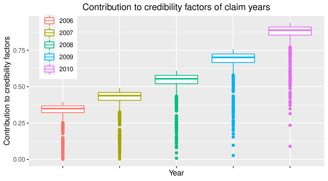
Figure 1: Contribution to credibility factors of past claim frequencies

Since $\widehat{\alpha}_{0}^{*}=\lambda_{T+1}-\sum_{t=1}^{T}\widehat{\alpha}_{t}\lambda_{t}=\lambda_{T+1}-\sum_{t=1}^{T}\widehat{\alpha}^{*}_{t}$, we have the following:

$${\rm Prem}\left(Y_{1},\cdots,Y_{T}\right) =\widehat{\alpha}^{*}_{0}+\sum_{t=1}^{T}\widehat{\alpha}_{t}^{*}Y_{t}^{*}=\lambda_{T+1}+\sum_{t=1}^{T}\widehat{\alpha}_{t}^{*}(Y_{t}^{*}-1)$$ (29)

$$=\lambda_{T+1}+\sum_{t=1}^{T}\widehat{\alpha}_{t}(Y_{t}-\lambda_{t})=\lambda_{T+1}\left(1+\sum_{t=1}^{T}\frac{\widehat{\alpha}_{t}}{\lambda_{T+1}}(Y_{t}-\lambda_{t})\right).$$

Therefore, one can interpret $1+\sum_{t=1}^{T}\frac{\widehat{\alpha}_{t}}{\lambda_{T+1}}(Y_{t}-\lambda_{t})$ as a posterior rating factor, which is multiplied by the prior premium to reflect past claims history with adjustments.

Figure 2 explains the behaviors of posterior rating factors depending on the number of past claims observed. First, those who had no claim at all in the past years would get sure discounts, which is considerably reasonable and agree with (29) as $Y_{t}-\lambda_{t}<0$ for all $t=1,\ldots,T$ in this case. One can also see that posterior rating factors tend to increase as a function of the numbers of past claims on average, which gives a motivation of risk mitigation and control to the policyholders for possible future discount. Further, interestingly, it is still possible to get discount even with a positive number of past claims as $Y_{t}-\lambda_{t}$ is not necessarily positive, especially when $\lambda_{t}$ is sufficiently large. Therefore, the given posterior ratemaking scheme still penalizes those who had claims in the past but in a relative manner and considering adjustments with varying levels of expected claims determined by observable characteristics.

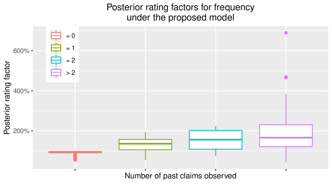
Figure 2: Distribution of posterior rating factor with past claim frequencies

In this sample study, the proposed dynamic credibility premium outperforms both the naive and static credibility premiums as shown in Table 7. This is in terms of both RMSE and MAE and even as good as the exact premium, which is obtained by 30,000 posterior sampling of the posterior rating factor via MCMC with substantial computation time reduction.

Table 7: Validation measures for the frequency models

	Naive	Static	Proposed	Exact
RMSE	0.6439	0.5002	0.4263	0.4661
MAE	0.1220	0.1121	0.1046	0.1060

6 Concluding remarks

In this study, we have examined the existence or the lack thereof of decreasing properties for the credibility coefficients in dynamic random effect models. We have shown that this is the case when the dynamic random effect process has an AR(1) type ACF and have found counter-examples when the ACF assumes some of the more general forms. Hence, for these models, credibility premium can be safely used, if the reader is unwilling to specify completely the dynamics of the random effect process for computational or robustness concerns. However, because the AR(1)-type ACF is a quite restrictive specification, the take-home message we want to convey is not necessarily to stick with AR(1)-type dynamic credibility models. Rather, we also want to bring this potential limitation of dynamic credibility to the attention of the actuarial community. In particular, one important open question is whether we can suitably extend the class of “admissible” ACF’s beyond the AR(1) case. Indeed, in the two counter-examples that we found, the dynamic random effect process has an unconstrained ACF, or is non-ergodic. In other words, we have not ruled out the possibility that other ergodic processes with non-AR(1) ACF could be compatible with decreasing credibility coefficients. For instance, some interesting candidate ACF’s to investigate would be those of ARFIMA(0,$d$,0)-type, which have recently been proved by Pinquet (2020b) to ensure at least the positivity of the credibilities. This is left for future research.

Appendix A Proof of Theorem 1

For expository purpose, let us first introduce some further notations. Define $T\times T$ diagonal matrices

$$\boldsymbol{\Lambda}_{T}={\rm diag}\left(\lambda_{1},\cdots,\lambda_{T}\right)\quad\hbox{and}\quad\boldsymbol{\Xi}_{T}={\rm diag}\left(\xi_{1},\cdots,\xi_{T}\right),$$

where

$$\xi_{t}:=\frac{\sigma^{2}\left(1-\rho^{2}\right)}{\psi}\frac{\left(\lambda_{t}\right)^{2}}{{\mathrm{E}}\left[V\left(\lambda_{t}R_{t}\right)\right]},\quad t=1,\ldots,T,$$

and define the $T\times T$ covariance matrix $\boldsymbol{\Sigma}_{T}$ of $\left(Y_{1:T}\right)$ as

$$\left[\boldsymbol{\Sigma}_{T}\right]_{t_{1},t_{2}}=\begin{cases}{\rm Cov}\left[Y_{t_{1}},Y_{t_{2}}\right],&t_{1}\neq t_{2};\\ {\mathrm{V}ar}\left(Y_{t_{1}}\right),&t_{1}=t_{2};\end{cases}$$

for $t_{1},t_{2}=1,\cdots,T$. Further, we define the following symbols, which are convenient to express the result on credibility premium for Model 1.

Definition 1.

For the given $\xi_{1},\ldots,\xi_{T}>0$ and $\rho\in(-1,1)$, define the sequences $\left(v_{1},\ldots,v_{T}\right)$ and $\left(u_{1},\ldots,u_{T}\right)$ as follows.

1. Define $d_{T}:=1+\xi_{T}$ and iteratively define

   $$d_{t}:=1+\rho^{2}+\xi_{t}-\frac{\rho^{2}}{d_{t+1}},\quad\hbox{for}\quad t=T-1,\ldots,2.$$

   Finally, define

   $$d_{1}:=1+\xi_{1}-\frac{\rho^{2}}{d_{2}}.$$

2. Define $v_{1}=1/d_{1}$ and iteratively define

   $$v_{t}:=\frac{\rho}{d_{t}}v_{t-1},\quad\hbox{for}\quad t=2,\ldots,T.$$

3. Define $\delta_{1}:=1+\xi_{1}$ and iteratively define

   $$\delta_{t}:=1+\rho^{2}+\xi_{t}-\frac{\rho^{2}}{\delta_{t-1}},\quad\hbox{for}\quad t=2,\ldots,T-1.$$

   Finally, define

   $$\delta_{t}:=1+\xi_{t}-\frac{\rho^{2}}{\delta_{t-1}}.$$

4. Define

   $$u_{T}=\frac{1}{\delta_{T}v_{T}},$$

   and iteratively define

   $$u_{t}:=\frac{\rho}{\delta_{t}}u_{t+1},\quad\hbox{for}\quad t=T-1,\ldots,1.$$

Simple calculation shows that $d_{t}>0$ for $t=2,\ldots,T-1$ so that the sequences $\left(v_{1},\ldots,v_{T}\right)$ and $\left(u_{1},\ldots,u_{T}\right)$ in Definition 1 are well-defined. The following lemma provides some more results on the sequences $\left(v_{1},\ldots,v_{T}\right)$ and $\left(u_{1},\ldots,u_{T}\right)$.

Lemma 1.

For the given $\xi_{1},\ldots,\xi_{t}>0$ and $\rho\in(-1,1)$, we have the following results on the sequences $\left(v_{1},\ldots,v_{T}\right)$ and $\left(u_{1},\ldots,u_{T}\right)$ in Definition 1.

1. $\left(v_{1:T}\right)$ is a decreasing sequence—$v_{t}\geq v_{t+1}$ for $t=1,\ldots,T-1$ where the equality holds for $\rho=0$.

2. $\left(u_{1:T}\right)$ is an increasing sequence—$u_{t}\leq u_{t+1}$ for $t=1,\ldots,T-1$ where the equality holds for $\rho=0$.

Proof.

To prove part i, it suffices to show that $\rho/d_{t}\leq 1$ for $t=2,\ldots,T$ by induction. First, one can easily see that $\rho/d_{T}=\rho/(1+\xi_{T})\leq 1$. Further, if $\rho/d_{k+1}\leq 1$, then

$$d_{k}-\rho=1+\rho^{2}-\rho+\xi_{k}-\frac{\rho^{2}}{d_{k+1}}=(1-\rho)^{2}+\xi_{k}+\rho\left(1-\frac{\rho}{d_{k+1}}\right)\geq 0,$$

which lead to $d_{t}\geq\rho$ for $t=2,\ldots,T-1$ and subsequently $\rho/d_{t}\leq 1$ for $t=2,\ldots,T-1$.

For part ii, one can prove that $\rho/\delta_{t}\leq 1$ for $t=1,\ldots,T-1$ in the same manner. ∎

We also provide new symbols and related properties that are useful in the calculation of credibility factors.

Definition 2.

Under the distributional assumption in Model 1, define a $T\times T$ diagonal matrix $\boldsymbol{Q}_{T}^{*}$ by

$$\boldsymbol{Q}_{T}^{*}:={\rm diag}\left(q_{1}^{*},\cdots,q_{T}^{*}\right)$$

, where $q_{t}^{*}:=\psi{\mathrm{E}}\left[V\left(\lambda_{t}R_{t}\right)\right]$. We further define a $T\times T$ matrix $\boldsymbol{\Sigma}_{T}^{*}$ by

$$\left[\boldsymbol{\Sigma}_{T}^{*}\right]_{i,j}=\begin{cases}1+\xi_{j},&(i,j)=(1,1)\quad\hbox{or}\quad(i,j)=(T,T);\\ 1+\rho^{2}+\xi_{j},&i=j,\quad(i,j)\neq(1,1)\quad\hbox{and}\quad(i,j)\neq(T,T);\\ -\rho,&j=i+1\quad\hbox{or}\quad j=i-1;\\ 0,&\hbox{otherwise.}\end{cases}$$

Note that the matrix $\boldsymbol{\Sigma}_{T}^{*}$ satisfies

$$\boldsymbol{\Sigma}_{T}^{*} =\left(1-\rho^{2}\right)\left(\boldsymbol{\Sigma}_{T,\rho}\right)^{-1}+\left(1-\rho^{2}\right)\sigma^{2}\boldsymbol{\Lambda}_{T}\left(\boldsymbol{Q}_{T}^{*}\right)^{-1}\boldsymbol{\Lambda}_{T}$$ (30)

$$=\left(1-\rho^{2}\right)\left(\boldsymbol{\Sigma}_{T,\rho}\right)^{-1}+\boldsymbol{\Xi}_{T}.$$

Lemma 2.

Under the settings in Model 1, we have

1. For a $T\times T$ matrix $\boldsymbol{\Sigma}_{T,\rho}$

   $$\left(1-\rho^{2}\right)\left(\boldsymbol{\Sigma}_{T,\rho}\right)^{-1}=\begin{cases}1,&(i,j)=(1,1)\quad\hbox{or}\quad(i,j)=(T,T);\\ 1+\rho^{2},&i=j,\quad(i,j)\neq(1,1)\quad\hbox{and}\quad(i,j)\neq(T,T);\\ -\rho,&j=i+1\quad\hbox{or}\quad j=i-1;\\ 0,&\hbox{otherwise.}\end{cases}$$ (31)

   and

   $$\left(\boldsymbol{\Sigma}_{T,\rho}\right)^{-1}\left(\rho^{T},\cdots,\rho^{1}\right)^{\prime}=\left(0,\cdots,0,\rho\right)^{\prime}$$ (32)

2. Moreover,

   $$\left(\boldsymbol{I}_{T}+\frac{1}{\sigma^{2}}\boldsymbol{Q}_{T}^{*}\left(\boldsymbol{\Lambda}_{T}\right)^{-1}\left(\boldsymbol{\Sigma}_{T,\rho}\right)^{-1}\left(\boldsymbol{\Lambda}_{T}\right)^{-1}\right)^{-1}=\sigma^{2}\left(1-\rho^{2}\right)\boldsymbol{\Lambda}_{T}\left(\boldsymbol{\Sigma}_{T}^{*}\right)^{-1}\boldsymbol{\Lambda}_{T}\left(\boldsymbol{Q}_{T}^{*}\right)^{-1}.$$

Proof.

The proof of (31) is from the well-known result on the inverse of AR(1) matrix $\boldsymbol{\Sigma}_{T,\rho}$. The result in (32) is the immediate result of (31). The proof of part ii is from (30) and the simple matrix algebra. ∎

Finally, we present the analytical expression for the credibility premium under the distributional assumption in Model 1.

Theorem 2.

Consider a state-space model comprising a state process $(R_{t}:t=0,1,\ldots)$ and observable time series $(Y_{t}:t=1,2,\ldots)$ in Model 1. Subsequently, the credibility premium defined in (19) has the following property.

1. $\widehat{\alpha}_{0}^{*},\cdots,\widehat{\alpha}_{T}^{*}$ in (20) can be expressed as

   $$\left(\widehat{\alpha}_{1}^{*},\cdots,\widehat{\alpha}_{T}^{*}\right)=\rho\left(1-\rho^{2}\right)\sigma^{2}\lambda_{T+1}v_{T}\left(u_{1}\frac{\lambda_{1}^{2}}{q_{1}^{*}},\cdots,u_{T}\frac{\lambda_{t}^{2}}{q_{T}^{*}}\right)$$

   and

   $$\widehat{\alpha}_{0}^{*}=1-\sum\limits_{t=1}^{T}\widehat{\alpha}_{t}^{*}.$$

   , where $(u_{1:T})$, $v_{T}$ are defined in Definition 1, and $(q^{*}_{1:T})$ is defined in Definition 2.

2. The credibility premium defined in (19) is regular.

Proof.

For convenience, we first show the representation for $\left(\widehat{\alpha}_{1},\cdots,\widehat{\alpha}_{T}\right)$. Subsequently, we can use the equation in (20). Following the classical procedure in Bühlmann and Gisler (2006), we have

$$\left(\widehat{\alpha}_{1},\cdots,\widehat{\alpha}_{T}\right)^{\prime} =\left(\boldsymbol{\Sigma}_{T}\right)^{-1}\left({\rm Cov}\left[Y_{1},Y_{T+1}\right],\cdots,{\rm Cov}\left[Y_{T},Y_{T+1}\right]\right)^{\prime}$$ (33)

$$=\sigma^{2}\lambda_{T+1}\left(\boldsymbol{Q}_{T}^{*}+\sigma^{2}\boldsymbol{\Lambda}_{t}\boldsymbol{\Sigma}_{T,\rho}\boldsymbol{\Lambda}_{T}\right)^{-1}\boldsymbol{\Lambda}_{T}\left(\rho^{T},\cdots,\rho^{1}\right)^{\prime}$$

and

$$\widehat{\alpha}_{0}=\lambda_{T+1}\left(1-\sum\limits_{t=1}^{T}\widehat{\alpha}_{t}\right).$$

For the further derivation of (33), we first investigate the auxiliary result on a symmetric tridiagonal matrix $\boldsymbol{\Sigma}_{T}^{*}$. Specifically, we have the following result on the inverse of symmetric tri-diagonal matrix (Meurant, 1992)

$$\left(\boldsymbol{\Sigma}_{t}^{*}\right)^{-1}\left(\begin{array}[]{c}0\\ \vdots\\ 0\\ 1\\ \end{array}\right) =\left(\begin{array}[]{ccccc}u_{1}v_{1}&u_{1}v_{2}&u_{1}v_{3}&\cdots&u_{1}v_{T}\\ u_{1}v_{2}&u_{2}v_{2}&u_{2}v_{3}&\cdots&u_{2}v_{T}\\ u_{1}v_{3}&u_{2}v_{3}&u_{3}v_{3}&\cdots&u_{3}v_{T}\\ \vdots&\vdots&\vdots&\ddots&\vdots\\ u_{1}v_{T}&u_{2}v_{T}&u_{3}v_{T}&\cdots&u_{T}v_{T}\\ \end{array}\right)\left(\begin{array}[]{c}0\\ \vdots\\ 0\\ 1\\ \end{array}\right)=v_{T}\left(\begin{array}[]{c}u_{1}\\ \vdots\\ u_{T}\\ \end{array}\right)$$ (34)

where $\left(u_{1:T}\right)$ and $\left(v_{1:T}\right)$ are defined in Definition 1.

Finally, we have

$$\left(\widehat{\alpha}_{1},\cdots,\widehat{\alpha}_{T}\right)^{\prime}$$

$$=\sigma^{2}\lambda_{T+1}\left(\boldsymbol{Q}_{T}^{*}+\sigma^{2}\boldsymbol{\Lambda}_{T}\boldsymbol{\Sigma}_{T,\rho}\boldsymbol{\Lambda}_{T}\right)^{-1}\boldsymbol{\Lambda}_{T}\left(\rho^{T},\cdots,\rho^{1}\right)^{\prime}$$

$$=\sigma^{2}\lambda_{T+1}\left(\boldsymbol{Q}_{T}^{*}\right)^{-1}\left(\boldsymbol{I}_{T}+\sigma^{2}\boldsymbol{\Lambda}_{T}\boldsymbol{\Sigma}_{T,\rho}\boldsymbol{\Lambda}_{T}\left(\boldsymbol{Q}_{T}^{*}\right)^{-1}\right)^{-1}\boldsymbol{\Lambda}_{T}\left(\rho^{T},\cdots,\rho^{1}\right)^{\prime}$$

$$=\lambda_{T+1}\left(\boldsymbol{Q}_{T}^{*}\right)^{-1}\left(\boldsymbol{I}_{T}+\frac{1}{\sigma^{2}}\boldsymbol{Q}_{T}^{*}\left(\boldsymbol{\Lambda}_{T}\right)^{-1}\left(\boldsymbol{\Sigma}_{T,\rho}\right)^{-1}\left(\boldsymbol{\Lambda}_{T}\right)^{-1}\right)^{-1}\boldsymbol{Q}_{T}^{*}\left(\boldsymbol{\Lambda}_{T}\right)^{-1}\left(\boldsymbol{\Sigma}_{T,\rho}\right)^{-1}\left(\rho^{T},\cdots,\rho^{1}\right)^{\prime}$$

$$=\rho\sigma^{2}\left(1-\rho^{2}\right)\lambda_{T+1}\left(\boldsymbol{Q}_{T}^{*}\right)^{-1}\boldsymbol{\Lambda}_{T}\left(\boldsymbol{\Sigma}_{t}^{*}\right)^{-1}\left(0,\cdots,0,1\right)^{\prime}$$

$$=\rho\left(1-\rho^{2}\right)\sigma^{2}\lambda_{T+1}v_{T}\left(u_{1}\frac{\lambda_{1}}{q_{1}^{*}},\cdots,u_{T}\frac{\lambda_{T}}{q_{T}^{*}}\right),$$

where the third equality is from Woodbury matrix identity (Hager, 1989; Higham, 2002), the fourth equality is from Lemma 2, and the final equality is from (34). Now, (20) concludes the proof of part i, and part ii immediately comes from part i. ∎

Finally, the proof of Theorem 1 follows immediately from Theorem 2.

Appendix B A heterogeneous INAR(1) model

Here, we investigate the ordering of credibility factors in the heterogeneous integer-valued autoregressive (INAR(1)) model proposed in Gourieroux and Jasiak (2004). Owing to its simple and intuitive structure, INAR(1) model is widely used in the modelling of the frequency in insurance literature (Boucher et al., 2008).

For a non-negative integer-valued random variable $Y$ and the constant $p\in[0,1]$, define the thinning operator $p\circ Y$ as follows: conditional on $Y$, $p\circ Y$ is a random variable distributed by ${\rm BN}\left(Y,p\right)$—the binomial distribution with size $Y$ and probability $p$.

Definition 3 (baseline or homogenous INAR(1) model).

Consider an autoregressive count model $\left(Y_{t};t=1,2,\cdots\right)$ such that $Y_{1}\sim{\rm Pois}(\frac{\lambda}{1-p})$, and for all $t>1$,

$$Y_{t}=p\circ Y_{t-1}+\epsilon_{t}$$ (35)

where $\epsilon_{t}$’s are i.i.d. observations drawn from ${\rm Pois}(\lambda)$. Furthermore, conditionally on $Y_{t-1}$, the random variable $p\circ Y_{t-1}$ is assumed to be independent from the sequence $\epsilon_{t}$. It has been shown by (McKenzie, 1985; Al-Osh and Alzaid, 1987) that this process is stationary and has AR(1)-like ACF as, by definition, $E[Y_{t}|Y_{t-1}]=pY_{t-1}+\lambda$.

Definition 4 (Heterogeneous INAR(1) model).

The heterogeneous INAR(1) model extends the above baseline INAR(1) model by allowing the parameter $\lambda$ to be heterogeneous across the population. More precisely, we say that $\left(Y_{t};t=1,2,\cdots\right)$ is heterogeneous INAR(1), if

1. given the unobservable heterogeneity factor $R$, the sequence $\left(Y_{t};t=1,2,\cdots\right)$ follows the INAR(1) process in (35), where conditional on the past observation $Y_{t-1},Y_{t-2},\cdots,Y_{1}$, variables $p\circ Y_{t-1}$ and $\epsilon_{t}$ are independent with distributions ${\rm BN}\left(Y_{t-1},p\right)$ and ${\rm Pois}\left(\lambda R\right)$, respectively.

2. The marginal distribution of $R$ is ${\rm Gamma}\left(1,\psi_{0}\right)$.

For the heterogeneous $INAR(1)$ in Model 1, as ${\mathrm{E}}\left[R\right]=1$, we still have

$${\mathrm{E}}\left[Y_{t}\right]=\frac{\lambda}{1-p}.$$

Moreover,

$${\rm Cov}\left[Y_{t},Y_{t+h}\right]=\frac{\lambda}{1-p}\left(p^{h}+\frac{\lambda}{1-p}\psi_{0}\right)\quad\hbox{and}\quad{\mathrm{V}ar}\left(Y_{t}\right)=\frac{\lambda}{1-p}\left(1+\frac{\lambda}{1-p}\psi_{0}\right)$$ (36)

Consequently, it satisfies the positive covariance ordering in (2). However, from Lemma 3 below, we have the ordering of credibility factors in (13) showing that the credibility factors do not satisfy the increasing property in (10).

Lemma 3.

Under the heterogeneous INAR(1) model in Definition 4, the credibility premium in (4) is obtained as

$$\widehat{\alpha}_{0}=\frac{\lambda\left(1-p^{2}\right)}{(1-p)\left(b(t-p(t-2))+1+p\right)}\quad\hbox{and}\quad\widehat{\alpha}_{1}=\frac{b(1-p)}{b(t-p(t-2))+1+p}$$ (37)

and

$$\widehat{\alpha}_{j}=\begin{cases}(1-p)\widehat{\alpha}_{1},&j=2,\cdots,t-1;\\ \widehat{\alpha}_{1}+p,&j=t;\\ \end{cases}$$ (38)

where

$$b=\frac{\lambda\psi_{0}}{1-p}.$$

Proof.

First, we calculate a covariance matrix, $\boldsymbol{\Sigma}_{t}$, of $\left(Y_{1},\cdots,Y_{t}\right)$ as

$$\boldsymbol{\Sigma}_{t}=\left(\frac{\lambda}{1-p}\right)^{2}\psi_{0}\boldsymbol{E}_{t}+\frac{\lambda}{1-p}\boldsymbol{\Sigma}_{t,p}.$$ (39)

Furthermore, by Sherman–Morrison formula (Sherman and Morrison, 1950; Press et al., 2007), observe the following matrix calculation

$$\left(\boldsymbol{\Sigma}_{t,p}+c\boldsymbol{E}_{t}\right)^{-1}=\left(\boldsymbol{\Sigma}_{t,p}\right)^{-1}{-}\frac{c}{1+c\boldsymbol{1}_{t}^{\mathrm{T}}\left(\boldsymbol{\Sigma}_{t,p}\right)^{-1}\boldsymbol{1}_{t}}\left(\boldsymbol{\Sigma}_{t,p}\right)^{-1}\boldsymbol{E}\left(\boldsymbol{\Sigma}_{t,p}\right)^{-1},$$ (40)

where

$$c=\frac{\lambda}{1-p}\psi_{0}.$$

Subsequently, by (3), (39), and (40), the credibility premium in (4) is obtained as in (37) and (38). ∎

Appendix C Results on the ordering of the credibility factors under specific variance functions

Corollary 1.

Consider the time series $(Y_{t})$ in the state-space model in Model 1. Subsequently, we have the following results regardless of the choice of $(\lambda_{t})$.

1. If we are given the following variance function

   $$V(x)=x$$

   of the EDF in (14), then the credibility factors satisfy

   $$\widehat{\alpha}_{1}\leq\cdots\leq\widehat{\alpha}_{T},$$

   where the equality holds if and only if $\rho=0$.

2. If we are given the following variance function

   $$V(x)=x^{2}$$

   of the EDF in (14), then the credibility factors corresponding to the standardized observations satisfy

   $$\widehat{\alpha}_{1}^{*}\leq\cdots\leq\widehat{\alpha}_{T}^{*},$$

   where the equality holds if and only if $\rho=0$.

The unit variance functions of Poisson and gamma distributions are given by $V(\mu)=\mu$ and $V(\mu)=\mu^{2}$, respectively. The following examples show that the numerical experiments on the ordering of the credibility factors confirm the results in Corollary 1.

Example 10.

In this example, under the settings in Example 7, we calculate the credibility factors of the non-standard observations, $(Y_{1},\cdots,Y_{T})$ with same parameters in Section 4.1. We note that the unit variance function of the Poisson distribution is given by the identity function. Consequently, Corollary 1 implies that the credibility factors of non-standard observations $(Y_{1},\cdots,Y_{T})$ are increasing regardless of the choice of $(\lambda_{t})$ as shown in Table 8.

Table 8: Credibility factors of the non-standardized observations in Example 10 (The credibility factors are written in the unit of $0.001$.)

	$\rho$	$(\lambda_{1},\cdots,\lambda_{5})$	$\widehat{\alpha}_{1}$	$\widehat{\alpha}_{2}$	$\widehat{\alpha}_{3}$	$\widehat{\alpha}_{4}$	$\widehat{\alpha}_{5}$
Case 1.a	0.3	$(1,1,1,1,1)$	0.167	0.809	3.999	19.785	97.894
Case 1.b	0.3	$(0.001,0.01,0.1,1,10)$	0.131	0.438	1.467	5.114	24.871
Case 1.c	0.3	$(10,1,0.1,0.01,0.001)$	0.131	2.430	12.384	44.442	149.765
Case 2.a	0.6	$(1,1,1,1,1)$	6.172	13.578	31.847	75.594	179.815
Case 2.b	0.6	$(0.001,0.01,0.1,1,10)$	4.586	7.646	12.785	22.016	48.859
Case 2.c	0.6	$(10,1,0.1,0.01,0.001)$	4.586	32.102	85.300	165.793	291.383

Example 11.

In this example, under the settings in Example 6, we calculate the credibility factors of the non-standard observations $(Y_{1},\cdots,Y_{T})$ and the standard observations $(Y_{1}^{*},\cdots,Y_{T}^{*})$, respectively, with $T=5$, $\sigma^{2}=0.5$, and $\psi=0.5$.

As the unit distribution function of the Gamma distribution is given by $V(\mu)=\mu^{2}$, Corollary 1 implies that the credibility factors of non-standard observations $(Y_{1}^{*},\cdots,Y_{T}^{*})$ are increasing regardless of the choice of $(\lambda_{t})$. Note that the credibility factors of standard observations are not necessarily increasing as shown in Table 9.

Table 9: Credibility factors of the standardized observations and non-standardized observations in Example 11 (The credibility factors are written in the unit of $0.001$.)

	$\rho$	$(\lambda_{1},\cdots,\lambda_{5})$	$\widehat{\alpha}_{1}$	$\widehat{\alpha}_{2}$	$\widehat{\alpha}_{3}$	$\widehat{\alpha}_{4}$	$\widehat{\alpha}_{5}$
Case 1.a	0.3	$(1,1,1,1,1)$	0.134	0.716	3.916	21.429	117.279
Case 1.b	0.3	$(0.001,0.01,0.1,1,10)$	0.134	0.072	0.039	0.021	0.012
	$\rho$	$(\lambda_{1},\cdots,\lambda_{5})$	$\widehat{\alpha}_{1}^{*}$	$\widehat{\alpha}_{2}^{*}$	$\widehat{\alpha}_{3}^{*}$	$\widehat{\alpha}_{4}^{*}$	$\widehat{\alpha}_{5}^{*}$
Case 2.a	0.3	$(1,1,1,1,1)$	0.134	0.716	3.916	21.429	117.279
Case 2.b	0.3	$(0.001,0.01,0.1,1,10)$	0.000	0.001	0.004	0.021	0.117

References

- Abdallah et al. (2016) Anas Abdallah, Jean-Philippe Boucher, and Hélène Cossette. Sarmanov family of multivariate distributions for bivariate dynamic claim counts model. Insurance: Mathematics and Economics, 68:120–133, 2016.
- Al-Osh and Alzaid (1987) MA Al-Osh and Aus A Alzaid. First-order Integer-valued Autoregressive (INAR()) Process. Journal of Time Series Analysis, 8(3):261–275, 1987.
- Bolancé et al. (2003) Catalina Bolancé, Montserrat Guillén, and Jean Pinquet. Time-varying credibility for frequency risk models: estimation and tests for autoregressive specifications on the random effects. Insurance: Mathematics and Economics, 33(2):273–282, 2003.
- Bolancé et al. (2007) Catalina Bolancé, Michel Denuit, Montserrat Guillén, and Philippe Lambert. Greatest accuracy credibility with dynamic heterogeneity: the harvey-fernandes model. Belgian Actuarial Bulletin, 7(1):14–18, 2007.
- Boucher and Pigeon (2018) Jean-Philippe Boucher and Mathieu Pigeon. A claim score for dynamic claim counts modeling. arXiv preprint arXiv:1812.06157, 2018.
- Boucher et al. (2008) Jean-Philippe Boucher, Michel Denuit, and Montserrat Guillén. Models of insurance claim counts with time dependence based on generalization of poisson and negative binomial distributions. Variance, 2(1):135–162, 2008.
- Brouhns et al. (2003) Natacha Brouhns, Montserrat Guillén, Michel Denuit, and Jean Pinquet. Bonus-malus scales in segmented tariffs with stochastic migration between segments. Journal of Risk and Insurance, 70(4):577–599, 2003.
- Bühlmann and Gisler (2006) Hans Bühlmann and Alois Gisler. A course in credibility theory and its applications. Springer Science & Business Media, 2006.
- Frees et al. (2016) Edward W Frees, Gee Lee, and Lu Yang. Multivariate frequency-severity regression models in insurance. Risks, 4(1):4, 2016.
- Gaver and Lewis (1980) Donald P Gaver and PAW Lewis. First-order autoregressive gamma sequences and point processes. Advances in Applied Probability, pages 727–745, 1980.
- Gerber and Jones (1973) Hans U Gerber and Donald A Jones. Credibility formulae with geometric weights. In Proceedings of the Business and Economic Section, American Statistical Association, volume 229, page 230, 1973.
- Gerber et al. (1975) HU Gerber, D Jones, et al. Credibility formulas of the updating type. Transactions of the Society of Actuaries, 27(1):31–52, 1975.
- Goulet (1998) Vincent Goulet. Principles and application of credibility theory. 1998.
- Gourieroux and Jasiak (2004) Christian Gourieroux and Joann Jasiak. Heterogeneous INAR(1) model with application to car insurance. Insurance: Mathematics and Economics, 34(2):177–192, 2004.
- Grunwald et al. (2000) Gary K Grunwald, Rob J Hyndman, Leanna Tedesco, and Richard L Tweedie. Theory & methods: Non-gaussian conditional linear AR(1) models. Australian & New Zealand Journal of Statistics, 42(4):479–495, 2000.
- Hager (1989) William W Hager. Updating the inverse of a matrix. SIAM review, 31(2):221–239, 1989.
- Harvey and Fernandes (1989) Andrew C Harvey and Clara Fernandes. Time series models for count or qualitative observations. Journal of Business & Economic Statistics, 7(4):407–417, 1989.
- Higham (2002) Nicholas J Higham. Accuracy and stability of numerical algorithms. SIAM, 2002.
- Jeong (2020) Himchan Jeong. Testing for random effects in compound risk models via Bregman divergence. ASTIN Bulletin: The Journal of the IAA, 50:777–798, 2020.
- Lewis et al. (1989) Peter AW Lewis, Edward McKenzie, and David Kennedy Hugus. Gamma processes. Stochastic Models, 5(1):1–30, 1989.
- Li et al. (2020) Hong Li, Yang Lu, and Wenjun Zhu. Dynamic bayesian ratemaking: A markov chain approximation approach. North American Actuarial Journal, pages 1–20, 2020.
- Lu (2018) Yang Lu. Dynamic frailty count process in insurance: a unified framework for estimation, pricing, and forecasting. Journal of Risk and Insurance, 85(4):1083–1102, 2018.
- McCullagh and Nelder (1989) Pa McCullagh and Ja Aa Nelder. Generalized Linear Models, second ed. Chapman and Hall, London, 1989.
- McKenzie (1985) Ed McKenzie. Some Simple Models for Discrete Variate Time Series. Journal of the American Water Resources Association, 21(4):645–650, 1985.
- Meurant (1992) Gérard Meurant. A review on the inverse of symmetric tridiagonal and block tridiagonal matrices. SIAM Journal on Matrix Analysis and Applications, 13(3):707–728, 1992.
- Pinquet (2020a) Jean Pinquet. Poisson models with dynamic random effects and nonnegative credibilities per period. ASTIN Bulletin, 50(2):585–618, 2020a.
- Pinquet (2020b) Jean Pinquet. Positivity properties of the arfima (0, d, 0) specifications and credibility analysis of frequency risks. Insurance: Mathematics and Economics, 95:159–165, 2020b.
- Pinquet et al. (2001) Jean Pinquet, Montserrat Guillén, and Catalina Bolancé. Allowance for the age of claims in bonus-malus systems. ASTIN Bulletin: The Journal of the IAA, 31(2):337–348, 2001.
- Press et al. (2007) William H Press, Saul A Teukolsky, William T Vetterling, and Brian P Flannery. Numerical recipes 3rd edition: The art of scientific computing. Cambridge university press, 2007.
- Rönnegård et al. (2010) Lars Rönnegård, Xia Shen, and Moudud Alam. hglm: A package for fitting hierarchical generalized linear models. The R Journal, 2(2):20–28, 2010.
- Sherman and Morrison (1950) Jack Sherman and Winifred J Morrison. Adjustment of an inverse matrix corresponding to a change in one element of a given matrix. The Annals of Mathematical Statistics, 21(1):124–127, 1950.
- Smith and Miller (1986) RL Smith and JE Miller. A non-gaussian state space model and application to prediction of records. Journal of the Royal Statistical Society: Series B (Methodological), 48(1):79–88, 1986.
- Sundt (1988) Bjørn Sundt. Credibility estimators with geometric weights. Insurance: Mathematics and Economics, 7(2):113–122, 1988.
- Sutradhar and Jowaheer (2003) Brajendra C Sutradhar and Vandna Jowaheer. On familial longitudinal poisson mixed models with gamma random effects. Journal of Multivariate Analysis, 87(2):398–412, 2003.